Dyonic BIon black hole in string inspired model

Abstract

We construct static and spherically symmetric particle-like and black hole solutions with magnetic and/or electric charge in the Einstein-Born-Infeld-dilaton-axion system, which is a generalization of the Einstein-Maxwell-dilaton-axion (EMDA) system and of the Einstein-Born-Infeld (EBI) system. They have remarkable properties which are not seen for the corresponding solutions in the EMDA and the EBI system. If solutions do not have both magnetic and electric charge, the axion field becomes trivial. In the electrically charged case, neither the extreme nor the BPS saturated solutions exist. Although we can take the zero horizon radius limit for any Born-Infeld (BI) parameter $b$, there is no particle-like solution. In the magnetically charged case, the extreme solution does exist for the critical BI parameter (or charge) $\sqrt{b}Q_{m}=1/2$. The critical BI parameter divides the solutions qualitatively. For $\sqrt{b}Q_{m}<1/2$, there exists a particle-like solution for which the dilaton field is finite everywhere, while the no particle-like solution exists and the solution in the $r_{h}\to 0$ limit becomes naked for $\sqrt{b}Q_{m}>1/2$. Though there is an extreme solution, the BPS saturated solution does not exist in this case. When the solutions have both magnetic and electric charge, we obtain the nontrivial axion field which plays an important role particularly for small black holes. Thermodynamical properties and the configuration of the dilaton field approach those in the magnetically charged case in the zero horizon limit, although gravitational mass does not. This is related to the nontrivial behavior of the axion field. We can prove that there is no inner horizon and that the global structure is the same as the Schwarzschild black hole in any charged case.

I Introduction

The pioneering theory of the non-linear electromagnetic field was formulated by Born and Infeld (BI) in 1934[1]. Surprisingly, it has been shown that BI action arises in string-generated corrections if one considers the coupling of an Abelian gauge field to an open bosonic string or an open superstring[2]. Moreover, the world volume action of a D-brane is described by a kind of non-linear BI action in the weak string coupling limit[3]. In this respect, there have been many investigations about BI action. For example, a particle-like solution (BIon) was constructed and its relation to the fundamental strings attached to the brane was discussed[4]. The BI action in a constant background of the Kalb-Ramond potential $B_{\mu\nu}$ turns out to be described by gauge theory in a flat noncommutative spacetime[5]. BIon in such a spacetime was also discussed recently[6]. Modification of light propagation is also important and the general geometric aspects including the BI action was discussed in Ref. [7]. Fluctuation around a nontrivial solution of BI action have a limiting speed given not by the Einstein metric but by the Boillat metric[8] which is conformal to the open string metric[9]. In general, characteristics of the wave exhibits bi-refrigence. The BI action is an exceptional theory which is free from this.

Some extensions of BI action to the non-Abelian gauge field has been considered, although it is not determined uniquely because of ambiguity in taking the trace of internal space[10]. Classical glueball solutions which were prohibited in the standard Yang-Mills theory were reported in Ref. [11]. They were also considered in the non-Abelian BI action with symmetrized trace and the dependence of their properties on the method of taking the trace and on gravity were discussed in Ref. [12]. Earlier work to consider Einstein gravity in the Abelian BI action was first done by Demianski[13]. Then self-gravitating particle-like solutions (EBIon)[14] and their black hole solutions (EBIon black hole) were calculated analytically under a static spherically symmetric ansatz[13, 15]. The extension to consider higher curvature gravity was considered in Ref. [16].

The non-linearity of the electromagnetic field may bring remarkable properties such as nonsingular black hole solutions satisfying the weak energy condition reported in [17, 18]. They are distinct from Bardeen black holes in the point that they appear as solutions in the Einstein equation with a nonvanishing matter field[19]. Although the singularity appears in the BI model, we can find an intrinsic difference from the Reissner-Nortström (RN) black hole concerning causal structure and black hole thermodynamics.

Since the BI system, however, has a string theoretical origin, it should include the dilaton and the antisymmetric Kalb-Ramond tensor field, which we call the axion field, as formulated in Ref. [20]. It is a direct extension of the Einstein-Maxwell-dilaton-axion (EMDA) system, where the famous black hole solution was found with the vanishing axion (i.e., in the EMD system) by Gibbons and Maeda, and independently by Garfinkle, Horowitz and Strominger (GM-GHS)[21]. The black hole solutions including the axion field were also reported in Ref. [22, 23]. In this paper, we investigate the particle-like and black hole solutions in the Einstein-Born-Infeld-dilaton-axion (EBIDA) system, which we call dilatonic EBIon (DEBIon) and dilatonic EBIon black hole (DEBIon black hole), respectively.

We studied such solutions only when they have either magnetic or electric charge and clarified the effect of the dilaton field as a first step in the previous work[24]. The magnetically charged solution and electrically charged solution have different properties because of the absence of electric-magnetic duality[25]. This system was modified to satisfy such duality[26], and solitons and black holes are also considered in that system[27]. Since the magnetic and electric charges are, however, not taken into account simultaneously in these analyses, the axion field becomes trivial by assuming a spherically symmetric ansatz. It is intriguing that the dyon solution with a trivial axion field has a different global structure and thermodynamical properties from the monopole case in the EMD system, while that with the nontrivial axion field has the same properties as the monopole case because of the SL($2$,R) duality in the EMDA system. Both BI systems are formulated, including the axion field, and we need to clarify their role. Motivated by these factors, we consider the dyonic black hole with a nontrivial axion field. We use the original action considered in Ref. [20]. Though this action loses electric-magnetic duality, this may be restored if we consider other elements such as higher derivative terms of the field strength $F$.

This paper is organized as follows. In Sec. II, we describe our model, basic equations and boundary conditions. We explain electrically charged solutions and magnetically charged solutions in Sec. III and IV, respectively. We observe that the thermodynamical properties are distinct in these two cases, which is caused by the effect of the dilaton field. In Sec. V, we consider a dyon solution with a nontrivial axion field. This has various interesting properties which were not seen in the monopole cases. In particular, even when the ratio of the electric charge to the magnetic charge is large, the solution does not approach the electrically charged one because of the nontrivial axion configuration. Moreover, when we consider the evaporation process of the black hole, it approaches the extreme solution for some mass scale and has a very low Hawking temperature. When the mass of the black hole shifts from this mass scale, it exhibits abrupt growth in temperature which eventually diverges in the zero horizon limit. We denote concluding remarks and future work in Sec. VI. Throughout this paper, we use the units $c=G=\hbar=1$.

II Model and Basic Equations

We start with the following action[28];

$$S=\int d^{4}x\sqrt{-g}\left[\frac{R}{2\kappa^{2}}-\frac{(\nabla\phi)^{2}}{\kappa^{2}}-\frac{1}{24\kappa^{2}}e^{-4\gamma\phi}H^{2}+L_{BI}\right],$$ (1)

where $\kappa^{2}:=8\pi$ and $\gamma$ is the coupling constant of the dilaton field $\phi$. The three rank antisymmetric tenser field is expressed as, $H=dB+\frac{1}{4}A\wedge F$.

$L_{BI}$ is the BI part of the Lagrangian which is written as

$$L_{BI}=\frac{be^{2\gamma\phi}}{4\pi}\left\{1-\sqrt{1+\frac{e^{-4\gamma\phi}}{2b}P-\frac{e^{-8\gamma\phi}}{16b^{2}}Q^{2}}\right\}\ ,$$ (3)

where $P:=F_{\mu\nu}F^{\mu\nu}$ and $Q:=F_{\mu\nu}\tilde{F}^{\mu\nu}$. A tilde denotes the Hodge dual. We can rewrite the three rank antisymmetric tenser field using a single pseudo scalar field $a$ (the axion field) as

$$H^{2}=6e^{8\gamma\phi}(\nabla a)^{2}-12e^{4\gamma\phi}aQ.$$ (4)

When we examine the electric and the magnetic monopole cases separately, the term $Q$ vanishes and eventually the axion field becomes trivial by assuming a spherically symmetric ansatz. But for the dyonic case, which has both electric and magnetic charges, the axion becomes nontrivial. We will treat these cases systematically. The BI parameter $b$ has the physical interpretation of a critical field strength. In the string theoretical context, $b$ is related to the inverse string tension $\alpha^{\prime}$ by $b^{-1}=(2\pi\alpha^{\prime})^{2}$. Notice that the action (1) is reduced to the EMDA system in the limit $b\rightarrow\infty$ and to the EBI system with the massless field for $\gamma=0$ and $a=0$. Here, we concentrate on the case $\gamma=1$ which is predicted from superstring theory and $\gamma=0$ for comparison.

We consider the metric of static and spherically symmetric,

$$ds^{2}=-f(r)e^{-2\delta(r)}dt^{2}+f(r)^{-1}dr^{2}+r^{2}{d\Omega_{2}}^{2}\ ,$$ (5)

where $f(r)=1-2m(r)/r$. The gauge potential has the following form:

$$A = -\frac{w_{1}(r)}{r}dt-w_{2}(r)\cos\theta d\varphi.$$ (6)

From the BI equation, we obtain that $w_{2}\equiv Q_{m}$ is constant and

$$\left(\frac{w_{1}}{r}\right)^{\prime}=-YQ_{e}e^{2\phi-\delta}\left[r^{4}+\frac{(YQ_{e})^{2}}{b}\right]^{-\frac{1}{2}},$$ (7)

where $Q_{e}:=w_{1}(\infty)$, $q:=Q_{e}/Q_{m}$ and $Y:=1-a/q$. A prime denotes a derivative with respect to $r$. From this equation, the electric field $E_{r}=-(w_{1}/r)^{\prime}$ does not diverge but takes a finite value at the origin. The maximum value is $E_{r}=\sqrt{b}$ in the EBI system. As we will see, the electric field vanishes at the origin in the EBIDA system by the nontrivial behavior of $\phi$. The potential $w_{1}$ is formally expressed as

$$w_{1}=-r\int^{r}_{0}YQ_{e}e^{2\phi-\delta}\left[r^{4}+\frac{(YQ_{e})^{2}}{b}\right]^{-\frac{1}{2}}dr,$$ (8)

where we put $rw_{1}(0)=0$ without loss of generality. By the above ansätze the basic equations with $\gamma=1$ are written as follows.

$$m^{\prime}=-U+\frac{r^{2}}{2}f\left[(\phi^{\prime})^{2}+\frac{e^{4\phi}}{4}(a^{\prime})^{2}\right],$$ (9)

$$\delta^{\prime}=-r\left[(\phi^{\prime})^{2}+\frac{e^{4\phi}}{4}(a^{\prime})^{2}\right],$$ (10)

$$\phi^{\prime\prime}=-\frac{2}{r}\phi^{\prime}+\frac{e^{4\phi}}{2}(a^{\prime})^{2}-\frac{2}{f}\left[\left(\frac{m}{r}+U\right)\frac{\phi^{\prime}}{r}-X\right],$$ (11)

$$a^{\prime\prime}=-2a^{\prime}\left(\frac{1}{r}+2\phi^{\prime}\right)-\frac{2}{f}\left[\left(\frac{m}{r}+U\right)\frac{a^{\prime}}{r}+2V\right],$$ (12)

where

$$U:=br^{2}e^{2\phi}\left\{1-\sqrt{\left(1+\frac{Q_{e}^{2}Y^{2}}{br^{4}}\right)\left(1+\frac{e^{-4\phi}Q_{m}^{2}}{br^{4}}\right)}\right\},$$ (13)

$$V:=\frac{e^{-2\phi}Q_{m}Q_{e}Y}{r^{2}\sqrt{r^{4}+\frac{(YQ_{e})^{2}}{b}}},$$ (14)

$$X:=be^{2\phi}\left[\sqrt{\frac{br^{4}+(Q_{e}Y)^{2}}{br^{4}+Q_{m}^{2}e^{-4\phi}}}\left(1+\frac{V^{2}}{b^{2}}\right)-1\right].$$ (15)

Note that by introducing the dimensionless variables $\bar{r}:=\sqrt{b}r$, $\bar{m}:=\sqrt{b}m$, $\alpha_{e}:=\sqrt{b}Q_{e}$ and $\alpha_{m}:=\sqrt{b}Q_{m}$, we find that the parameters of the equation system are $\alpha_{e}$ and $\alpha_{m}$. As we already explained, since this system loses electric-magnetic duality, when we obtain the black hole solution with electric charge in the above action, we can not transform it to the solution with magnetic charge by duality.

The boundary conditions at spatial infinity to satisfy the asymptotic flatness are

$$m(\infty)=:M=const.,\ \ \delta(\infty)=0,$$ (16)

$$\phi(\infty)=0,\ \ a(\infty)=0.$$ (17)

We also assume the existence of a regular event horizon at $r=r_{h}$ for the DEBIon black hole. So we have

$$m_{h}=\frac{r_{h}}{2},\;\;\delta_{h}<\infty,\;\;\phi_{h}<\infty,\;\;$$ (18)

$$\phi^{\prime}_{h}=\frac{2r_{h}X_{h}}{1+2U_{h}},\;\;\;a_{h}^{\prime}=\frac{-4r_{h}V_{h}}{1+2U_{h}}.$$ (19)

The variables with subscript $h$ mean that they are evaluated at the horizon. We will obtain the black hole solution numerically by determining $a_{h}$ and $\phi_{h}$ iteratively to satisfy these conditions.

To determine the boundary values of $\phi_{h}$ and $a_{h}$, it is convenient to rewrite the field equations (11) and (12) as follows,

$$(fe^{-\delta}r^{2}\phi^{\prime})^{\prime}=\frac{1}{2}fr^{2}e^{4\phi-\delta}(a^{\prime})^{2}+2r^{2}e^{-\delta}X,$$ (20)

$$(fe^{4\phi-\delta}r^{2}a^{\prime})^{\prime}=-4r^{2}e^{4\phi-\delta}V.$$ (21)

We first concentrate on the equation of the axion field. When the solution does not have both electric and magnetic charges, $A:=fe^{4\phi-\delta}r^{2}a^{\prime}=const.$ by (21). Since $A=0$ at the horizon, $a(r)^{\prime}\equiv 0$ can be derived which means $a\equiv 0$ to satisfy $a(\infty)=0$. In the dyon case, since the difference of the sign of $Q_{m}Q_{e}$ only affects the sign of $a$ as is seen in Eqs. (9)-(12), we restrict $Q_{m}Q_{e}>0$ below without loss of generality. Assuming $a_{h}>q$, we obtain $A^{\prime}>0$ that follows $A>0$ outside the horizon. Thus, $a$ increases monotonically and cannot satisfy $a(\infty)=0$. Assuming $a_{h}<q$, we obtain $A^{\prime}<0$ that follows $A<0$ outside the horizon. Thus, $a$ decreases monotonically and hence $0<a_{h}<q$ to satisfy $a(\infty)=0$. In this case, since we have $A>0$ (nonzero) inside the horizon, $f$ cannot become zero. So there is no inner horizon for the dyon case.

We consider the equation of the dilaton field (20). For the electrically charged case, we obtain $(fe^{-\delta}r^{2}\phi^{\prime})^{\prime}>0$ because $X(r\neq 0)>0$ and $a(r)^{\prime}\equiv 0$. Thus $C:=fe^{-\delta}r^{2}\phi^{\prime}<0$ and $C>0$ inside and outside the horizon, respectively. So $\phi^{\prime}>0$ everywhere and $f$ cannot become zero inside the horizon, i.e., there is no inner horizon. To satisfy $\phi(\infty)=0$, we should choose as $\phi_{h}<0$. We can discuss the magnetically charged case in the same way and find that $\phi_{h}>0$ and that there is no inner horizon. For the dyonic case, however, the sign of $X$ cannot be fixed since it depends not only on the charge ratio $q$ but also on the values $a_{h}$ and $\phi_{h}$ in a complex relationship.

We obtained solutions numerically. For the $b\to\infty$ case, we have a GM-GHS solution. This does not guarantee an existence of a solution for finite $b$. First, we show the necessary condition for the existence of a solution. To satisfy $m^{\prime}_{h}<1/2$, we have

$$4bQ_{e}^{2}Y_{h}^{2}e^{4\phi_{h}}-4br_{h}^{2}e^{2\phi_{h}}+4bQ_{m}^{2}$$ (22)

$$-1+\frac{4Q_{e}^{2}Q_{m}^{2}Y_{h}^{2}}{r_{h}^{4}}:=K<0.$$ (23)

If we see the equation $K=0$ as the second order equation for $e^{2\phi_{h}}$, following condition will be required from its discriminant.

$$br_{h}^{4}>Q_{e}^{2}Y_{h}^{2}\left[4Q_{e}^{2}\left(b+\frac{Q_{e}^{2}Y_{h}^{2}}{r_{h}^{4}}\right)-1\right].$$ (24)

Thus, for the existence of the solution in the $r_{h}\to 0$ limit, $Y_{h}/r_{h}^{2}$ should approach finite value ($0$ in our calculation) in this limit, which becomes important in Sec. V. Though, (23) is a necessary condition, when the conditions (23), (18), and (19) are satisfied, our calculation shows that the matter and the gravitational fields satisfy asymptotically flatness. This is plausible since the EBIDA system approaches the EMDA system for $r\to\infty$.

III Electrically charged solution

First, we investigate the electrically charged case. Before proceeding to the DEBIon black hole, we briefly review the solutions in the EBI system ($\phi\equiv a\equiv 0$). In the $b\to\infty$ limit, the EBI system reduces to the Einstein-Maxwell system. For finite $b$, we obtain EBIon and its black hole solutions analytically[13, 15]. We plot the $M$-$r_{h}$ relation in Fig. 1 by dot-dashed lines. The solution branches are divided qualitatively by $\alpha_{e}=\alpha^{\ast}:=1/2$. For $\alpha_{e}>\alpha^{\ast}$, there is a special value $M_{0}$ of which the analytic form is seen in Ref. [15]. For $M<M_{0}$ the black hole and inner horizon exist as the RN black hole while only the black hole horizon exists for $M\geq M_{0}$. The minimum mass solution in each branch corresponds to the extreme solution. On the other hand, all the black hole solutions have only one horizon and the global structure is the same as the Schwarzschild black hole for $\alpha_{e}<\alpha^{\ast}$. In this case, there exists EBIon solution with no horizon in the $r_{h}\to 0$ limit. Note however that, since $m^{\prime}(0)=\alpha_{e}$, it has the conical singularity at the origin, which is the characteristic feature of the self-gravitating BIons. For $\alpha_{e}=\alpha^{\ast}$, the extreme solution is realized in the $r_{h}\to 0$ limit. Although Demianski called it an electromagnetic geon [13] which is regular everywhere, it has a conical singularity like the other EBIons.

Next we turn to the $\gamma=1$ case. In the $b\to\infty$ limit, i.e., in the EMD system, the GM-GHS solution exists. The GM-GHS solution has three global charges, mass $M$, the electric charge $Q_{e}$ and the dilaton charge $\Sigma$. The dilaton charge depends on the former two, hence it is classified as a secondary charge[29]. For the GM-GHS solution, it is expressed as

$$\Sigma=-\frac{Q_{e}^{2}}{2M}.$$ (25)

There is no particle-like solution in this system.

For the finite value of $b$, we can not find the analytic solution and have to use numerical analysis. Since there is no non-trivial dilation configuration in the $Q_{e}=0$ case, the dilaton hair is again the secondary hair in this system. We plot the $M$-$r_{h}$ relation of the DEBIon black hole in Fig. 1 by solid lines. We can find that all branches reach to $r_{h}=0$ in contrast to the EBIon case. We examine the existence of the extremal solution. It has a degenerate horizon, where $2m^{\prime}=1$ is realized. Hence, by Eq. (9)

$$\alpha_{e}=\alpha_{e}^{ext}:=e^{-2\phi_{h}}\sqrt{\frac{1}{4}+br_{h}^{2}e^{2\phi_{h}}}.$$ (26)

Since $\phi_{h}=0$ in the EBI system, the extreme solutions exist for $\alpha_{e}\geq\alpha^{\ast}$. In this case, (26) is satisfied when $r_{h}=\sqrt{(\alpha_{e}^{2}-1/4)/b}$. For the EBID system, since $\phi_{h}$ diverges to minus infinity in the $r_{h}\to 0$ limit as we will see below, $\alpha_{e}^{ext}\to\infty$ and no extreme solution exists for finite $\alpha_{e}$.

As for the particle-like solution, we have to analyze this carefully. We employ a new function $\psi:=e^{2\phi}$ and expand the field variables as

$$\psi=\sum_{\alpha,\;\beta}\psi_{(\alpha,\beta)}r^{\alpha}(\ln r)^{\beta},\;\;\;\;m=\sum_{\gamma,\;\delta}m_{(\gamma,\delta)}r^{\gamma}(\ln r)^{\delta}.$$ (27)

Substituting them into the field equations and evaluating the lowest order equations, we find

$$\phi\sim-\frac{1}{2}\ln(-4\sqrt{bQ_{e}^{2}}\ln r),$$ (28)

$$m\sim-\frac{r}{4\ln r}.$$ (29)

The diverging behavior of the dilaton field is important. Though it is admissible as a particle-like solution in the sense of Ref. [14], conformal transformation back to the original string frame becomes singular. In this respect, we use the word a particle-like solution below for the solution which satisfies both the criterion [14] and the finiteness of the dilaton field.

From Fig. 1, we can find that the mass of the black hole becomes small when we include the dilaton field into the system for any value of BIon parameter $b$. The reason is clarified by examining the mass distribution. We show the mass distribution $r$-$m(r)$ of the electrically charged DEBIon black holes with $Q_{e}=0.1$, $r_{h}=0.04$ and $b=20$ and $25$ in Fig. 2. These configurations show how the dilaton field contributes to the mass function when we compare it to the EBIon black hole case. Roughly speaking, the contribution comes from two factors: (i) the dilaton coupling prefactor $e^{2\phi}$ which appears in Eq. (13) and (ii) the gradient term $(\phi^{\prime})^{2}$. Since $\phi$ takes negative value in the electrically charged case, factor (i) reduces the gravitational constant effectively. On the other hand, the second factor makes positive contribution to the mass function. We can find that factor (i) overcomes factor (ii), since gravitational mass is reduced compared with the one having no dilaton field. This effect appears particularly near the horizon where the dilaton field largely deviates from zero.

We show the relation between the horizon radius $r_{h}$ and $\phi_{h}$ in Fig. 3. We can find qualitative difference of the scalar field in the $r_{h}\to 0$ limit between the DEBIon black hole and the GM-GHS solution. The dilaton field of the GM-GHS solution diverges as

$$\phi_{h}\sim\ln\left(\frac{Mr_{h}}{Q_{e}^{2}}\right)\;\;\;\;(r_{h}\to 0).$$ (30)

At first glance, it seems that $\phi_{h}$ remains finite in the $r_{h}\to 0$ limit in the DEBIon black hole. This is due to the very small diverging rate

$$\phi_{h}\sim-\frac{1}{2}\ln(-4\sqrt{bQ_{e}^{2}}\ln r_{h}).$$ (31)

This relation is the same as in Eq. (28). The reason for this coincidence is unclear. The difference in the divergence rate between the GM-GHS and DEBIon black holes is a crucial point for thermodynamical behaviors and non-existence of the extreme solution.

We are also interested in the scalar field outside or inside the horizon. By integrating from the event horizon to spatial infinity, we can find monotonic behavior in the scalar field for a DEBIon black hole, which has a common property with the GM-GHS solution, as we showed in Sec. II. Even small black holes have a structure of the dilaton field which spreads out to infinity. This is related to the fact that the dilaton charge $\Sigma$ can be defined by

$$e^{-2\phi}\sim 1+\frac{2\Sigma}{r},\;\;\;\ \ (r\to\infty).$$ (32)

Though the dilaton field has a similar structure near infinity in both cases, independently of the size of the event horizon, it has an intrinsic difference at the small scale. It behaves as Eq.(30), which is not restricted at the horizon but holds everywhere in small scale here, and Eq.(28) for the GM-GHS solution and the DEBIon black hole, respectively.

Though the small scale behavior of the dilaton field is different from the GM-GHS case, we may wonder if relation (25) holds even for the DEBIon black hole. We show the relation $M$-$\Sigma$ of the electrically charged DEBIon black holes (solid lines) with $Q_{e}=0.1$ and $b=50$ and $500$ in Fig. 4. We also plotted the GM-GHS solution by a dotted line. This diagram shows that the relation (25) is violated for finite $b$ and absolute value of the dilaton charge for the DEBIon black hole is larger than that for the GM-GHS solution in the $r_{h}\to 0$ limit. Moreover, $|\Sigma|$ becomes larger than the gravitational mass $M$ in this limit and the solution does not correspond to the BPS saturated state, i.e.,

$$M^{2}+\Sigma^{2}=Q_{e}^{2}.$$ (33)

This is the same result in Ref.[27] considered in the slightly different model from ours.

As we showed in Sec. II, there is no inner horizon. By integrating from the event horizon toward the origin with suitable boundary conditions, we can examine the internal structure of the black hole. The dilaton field monotonically decreases and diverges as $\sim\ln r$. The electric field vanishes, approaching to the origin by the divergence of the dilaton field, as we show in Fig. 5. We choose $b=100$ and $r_{h}=0.4$. The mass function $m$ also diverges as $\approx r^{-x}$, $(0<x<1)$. Hence, the function $f$ does not have zero except at the event horizon. As a result, the global structure is Schwarzschild type.

By using Eq. (9), the temperature of the DEBIon black holes is expressed by

$$T = \frac{e^{-\delta_{h}}}{4\pi r_{h}}(1+2U_{h}).$$ (34)

It was shown that the thermodynamical properties change drastically in the $b\to\infty$ limit by putting the dilaton field on the black hole as seen in Fig. 6. The DEBIon black hole always has a higher temperature than the GM-GHS solution ($T=1/8\pi M$) because of the nonlinearity of the BI field. Since the EBIon black hole has the extreme limit, the temperature becomes zero in this limit for $\alpha_{e}>\alpha^{\ast}$. On the other hand, since there is no extreme solution for DEBIon black holes, their temperature does not vanish but diverges in the $r_{h}\to 0$ limit. Hence the evolution by the Hawking evaporation does not stop until the singular solution with $r_{h}\to 0$ when the surrounding matter field does not exist.

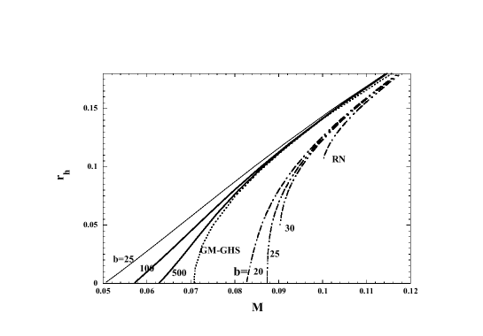
FIG. 1.: $M$-$r_{h}$ diagram of electrically charged DEBIon black holes (solid lines) with electric charge $Q_{e}=0.1$ and $b=25$, $100$ and $500$. GM-GHS and EBIon black holes are also plotted by a dotted line and dot-dashed lines, respectively.

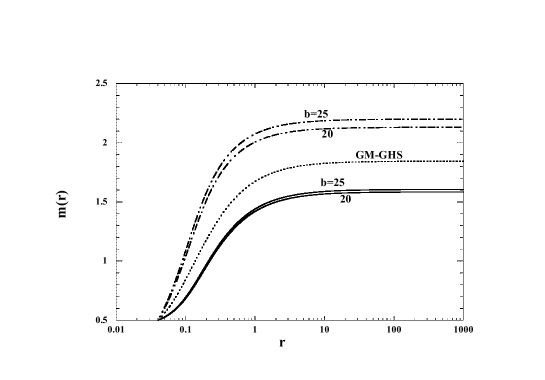
FIG. 2.: The mass distribution of the electrically charged DEBIon black holes (solid lines) with $Q_{e}=0.1$, $r_{h}=0.04$ and $b=25$ and $20$. GM-GHS and EBIon black holes cases are also plotted by a dotted line and dot-dashed lines, respectively.

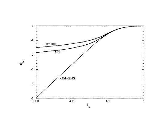
FIG. 3.: $r_{h}$-$\phi_{h}$ relation of electrically charged DEBIon black holes (solid lines) with $Q_{e}=0.1$ and $b=100$ and $500$. The GM-GHS solution is plotted by a dotted line. This diagram shows the qualitative difference of the divergence rate in the $r_{h}\to 0$ limit between the DEBIon black hole and the GM-GHS solution.

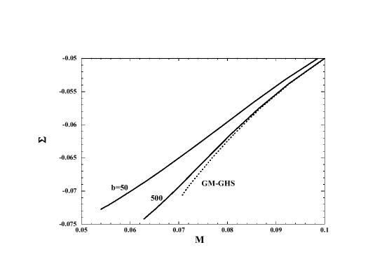
FIG. 4.: $M$-$\Sigma$ diagram of electrically charged DEBIon black holes (solid lines) with $Q_{e}=0.1$ and $b=50$ and $500$. The GM-GHS solution is plotted by a dotted line. This diagram shows that the relation (25) for GM-GHS solution is violated for finite $b$.

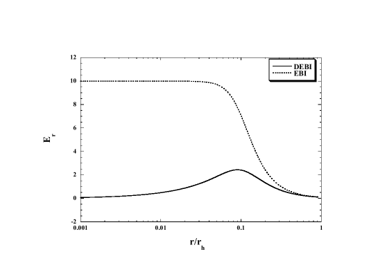
FIG. 5.: The distribution of the electric field $E_{r}$ diagram of electrically charged DEBIon black hole (solid line) and EBIon black hole (dotted line) for $r_{h}=0.4$ and $b=100$. Note that the central part of the DEBIon black hole is neutral because of the dilaton field. This is one of the reasons why the solution has a Schwarzschild type global structure.

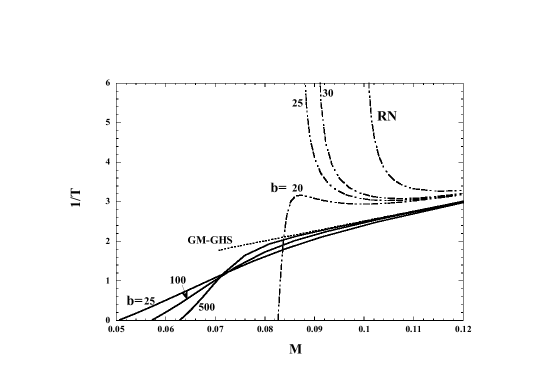
FIG. 6.: $M$-$1/T$ diagram of electrically charged DEBIon black holes (solid lines) and EBIon black holes (dot-dashed lines) with the same parameters in Fig. 1.

IV Magnetically charged solution

EBIon and GM-GHS black holes with magnetic charge can be obtained from their electrically charged counterparts owing to duality as $F\to\tilde{F}$, and $F\to e^{-2\phi}\tilde{F}$, $\phi\to-\phi$, respectively. Hence the relations $M$-$r_{h}$ and $M$-$1/T$ never change. As is noted above, however, our DEBIon system has no such duality. Then it is natural to expect that the magnetically charged solutions have different properties from electrically charged ones discussed in the previous section.

We show $M$-$r_{h}$ and $M$-$1/T$ relations in Fig. 7 and Fig. 8, respectively. Although the $M$-$r_{h}$ relation seems similar to that of the GM-GHS solution regardless of $\alpha_{m}$, the $M$-$1/T$ relation is different depending on $\alpha_{m}$. This is due to the qualitative difference of the behavior of the dilaton field in the $r_{h}\to 0$ limit. For $\alpha_{m}\geq\alpha^{\ast}$, the dilaton field diverges at the horizon as $\phi_{h}\sim\ln r_{h}$ and $\delta_{h}\sim-\ln r_{h}$, and hence the temperature remains finite as in the GM-GHS case. On the other hand, $\phi_{h}$ and $\delta_{h}$ are finite for $\alpha_{m}<\alpha^{\ast}$. As a result, the temperature diverges. Note that the corresponding solution is the particle-like solution.

We show the field distribution $r$-$\phi(r)$ of DEBIon and DEBIon black holes with $Q_{m}=0.1$ and $b=20$ in Fig. 9. For reference, we also plot the corresponding DEBIon black hole with $b=30$ by dotted lines. Note that while $\phi_{h}^{\prime}\to 0$ and $\phi_{h}$ remains finite in the $r_{h}\to 0$ limit with $b=20$, they do not when $b=30$. This is the most crucial difference which determines whether a particle-like solution exists or not. Since the dilaton field is finite everywhere, the particle-like solution is also relevant in the original string frame. Hence, in the magnetically charged case, DEBIon solution does exist for $\alpha_{m}<\alpha^{\ast}$.

We want to know whether or not the solutions in the $r_{h}\to 0$ limit correspond to the extreme ones. From Eq. (9),

$$\alpha_{m}=\alpha_{m}^{ext}:=\sqrt{\frac{1}{4}+b\Phi_{h}}$$ (35)

for the extreme solutions. Here $\Phi_{h}:=r_{h}^{2}e^{2\phi_{h}}$. Thus, there is no extreme solution for $\alpha_{m}<1/2$. For $\alpha_{m}\geq 1/2$, we must survey $\Phi_{h}$ (i.e., $\phi_{h}$). We show the relation $r_{h}$-$\Phi_{h}$ in Fig. 10. For $\alpha_{m}=\alpha^{\ast}$, because $\Phi_{h}\to 0$ as $r_{h}\to 0$, the extreme solution is realized in the $r_{h}\to 0$ limit, i.e., $\alpha_{m}=\alpha_{m}^{ext}$. For $\alpha_{m}>\alpha^{\ast}$, $\Phi_{h}\to const.\neq 0$ as $r_{h}\to 0$. We cannot tell whether Eq. (35) is fulfilled for a certain horizon radius since $\phi_{h}$ is obtained iteratively only by numerical method. Our calculation always shows $\alpha_{m}<\alpha_{m}^{ext}$ except for $\alpha_{m}=\infty$, which implies that the extreme solution is realized only when $\alpha_{m}=\alpha^{\ast}$ and $\alpha_{m}=\infty$. We also show the result for $\alpha_{m}<\alpha^{\ast}$ for reference. In this case, $\Phi_{h}\propto r_{h}^{2}$ in the $r_{h}\to 0$ limit. This shows that $\phi_{h}$ converges to finite value in this limit.

As we considered in the electrically charged case, we can divide the contributions from the dilaton field to the mass function. They are, however, more complicated than in the electrically charged case: (i) and (ii) are the same and there is another factor (iii) the prefactor $e^{-4\phi}$ before $Q_{m}^{2}$ in Eq. (13). Since both factors (i) and (ii) make positive contributions to the mass function because $\phi>0$, one may think that the gravitational mass becomes larger than the corresponding EBIon and EBIon black hole. But this is not the case. The third factor makes that the effect of the magnetic charge reduce by $e^{-4\phi}$, which forces the solution to approach the Schwarzschild one. As a result, the gravitational mass is reduced compared to the EBIon black hole.

We may think the effect of the dilaton field also makes a qualitative difference for the dilaton charge. We show the $M$-$\Sigma$ relation of a DEBIon black hole with $Q_{m}=0.1$ and $b=20$ and $30$. in Fig. 11. We can find that a qualitative difference near the horizon does not cause strong influence on the asymptotic region. Contrary to the electrically charged case, the dilaton charge of the DEBIon black hole is smaller than that of the GM-GHS solution in the $r_{h}\to 0$ limit. There is no BPS saturated solution in this case, either.

The behaviors of the field functions inside the event horizon are similar to those in the electrically charged case qualitatively, except for the sign of the dilaton field. The magnetic field diverges as $B_{r}\approx r^{-x}$, $(1<x<2)$. As we showed in Sec. II, there is no inner horizon and the dilaton field monotonically increases toward the origin. The nonexistence of the inner horizon is a characteristic feature of the black hole solution with a scalar field except for some special cases. The equations of the scalar fields become singular on the horizon where $f=0$, and the scalar field must satisfy a certain boundary condition there. However, when we integrate the scalar field equation from the black hole event horizon inward, this boundary condition can not be fulfilled in general and the scalar field diverges. As a result, there is no inner horizon. It may seem strange that there should be an extreme solution in spite of the fact that there is no inner horizon. In the EMD system, this can be understood as follows. The GM-GHS solution with the monopole charge has no inner horizon. But if we consider the dyon case in the EMD system, i.e., trivial axion, there appears an inner horizon. This corresponds to the special case. The inner horizon shrinks to $r\to 0$ in the limiting case, i.e., $Q_{e}=0$ or $Q_{m}=0$. The inner horizon and the event horizon can degenerate at $r=0$ when $M=\sqrt{2}Q_{e(m)}$. Thus, the extreme solution for the electrically (or magnetically) charged solution appears. In our case, we may think that only the magnetically charged solution corresponds to such a case.

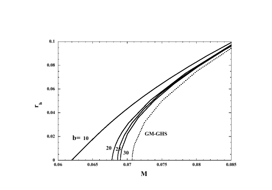
FIG. 7.: $M$-$r_{h}$ diagram of magnetically charged DEBIon black holes (solid lines) with magnetic charge $Q_{m}=0.1$ and $b=10$, $20$, $25$ and $30$. The GM-GHS black hole is also plotted by a dotted line.

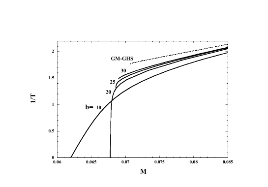
FIG. 8.: $M$-$1/T$ diagram of magnetically charged DEBIon black holes (solid lines) with the same parameters in Fig. 7.

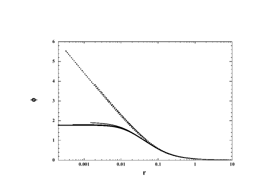
FIG. 9.: The field distribution $r$-$\phi(r)$ of magnetically charged DEBIon and DEBIon black holes with $Q_{m}=0.1$ and $b=20$ by solid lines. The horizon radii are choosen as $r_{h}=1.685\times 10^{-4}$, $4.918\times 10^{-4}$ and $1.499\times 10^{-3}$. We also plotted DEBIon black holes with $b=30$ by dotted lines. The horizon radii are choosen as $r_{h}=3.522\times 10^{-4}$, $1.996\times 10^{-3}$ and $9.564\times 10^{-3}$. When the particle-like solution exists, $\phi_{h}^{\prime}\to 0$ in the $r_{h}\to 0$ limit and $\phi$ does not diverge.

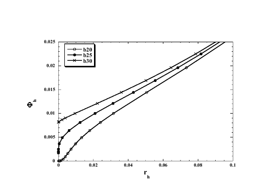
FIG. 10.: $r_{h}$-$\Phi_{h}$ diagram of magnetically charged DEBIon black holes for $b=20$, $25$ and $30$. This shows an intrinsic difference between $b=25$ and $30$ which determines whether the extreme solution exists or not . For $b=20$, since $\phi_{h}$ itself converges to nonzero value in the $r_{h}\to 0$ limit, $\Phi_{h}$ behaves as $\propto r_{h}^{2}$ in this limit.

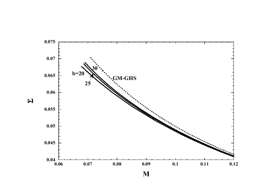
FIG. 11.: $M$-$\Sigma$ diagram of magnetically charged DEBIon black holes with $Q_{m}=0.1$ and $b=20$, $25$ and $30$ by solid lines. We also plotted the GM-GHS solution by dotted line.

V dyon solution

Finally, we investigate the dyon solutions which have both electric and magnetic charges. The dyon solution is important for the following reasons. In the EMD system, the black hole solutions have different properties from the monopole case. For example, there is an inner horizon and the global structure is the RN type[21, 30]. The inner horizon shrinks to zero in the monopole ($Q_{m}\to 0$ or $Q_{e}\to 0$) limit. The temperature becomes zero in the extreme limit while it is finite in the monopole cases. On the contrary, the dyoic black hole solution in the EMDA system can be obtained from the monopole one because of the SL($2$,R) duality [23]:

$$\lambda\to\frac{a\lambda+b}{c\lambda+d},\ \ \ \ ad-bc=1,$$ (36)

$$F_{+}\to-\lambda F_{+},\ \ \ \ F_{-}\to-\bar{\lambda}F_{-},$$ (37)

where $\lambda:=a+ie^{-2\phi}$, $F_{\pm}:=F\pm i\tilde{F}$ and $\bar{z}$ means the complex conjugate of $z$. This is why the temperature and inner structure coincide with the monopole case. We expect similar properties in the modified EBIDA model which has SL($2$,R) duality. However, since we treat the model without such duality, we can expect that nontrivial changes occur in our system and that the monopole solutions are its special cases. Moreover, we are interested in the effect of the axion field which was not investigated before. Since we find a trivial value for the monopole solutions under the static and spherically symmetric ansatz, we should by all means investigate the dyon solution. It may result in significant differences in such aspects as the behavior of the dilaton field or in the temperature.

We first show the $M$-$r_{h}$ relation of dyon solutions with $\sqrt{Q_{e}^{2}+Q_{m}^{2}}=0.1$ and $b=30$. We plot the solutions with $q\geq 1$ in Fig. 12 (a). Since dyon solutions in the EBI system and in the EMDA system have the same $M$-$r_{h}$ relations, we omit them. We also plot the solutions $q\leq 1$ in Fig. 12 (b). In the EMD system, solutions approach the electrically charged (or magnetically charged) ones in the $q\to\infty$ (or $\to 0$) limit. We can find, however, that the solutions with large $q$ do not approach the electrically charged case while those with small $q$ approach the magnetically charged case. This is due to the nontrivial distribution of the axion field. To see this, we investigate the scalar field of the small black hole solutions. Our numerical analysis shows that while $\phi_{h}$ increases as $r_{h}$ decreases for $r_{h}\mbox{\raisebox{-4.30554pt}{$\stackrel{{\scriptstyle\textstyle>}}{{\textstyle\sim}}$}}10^{-3}$, it decreases in the $r_{h}\to 0$ limit and $\phi_{h}^{\prime}$ approaches zero. This may seem to be the symptom of the existence of the particle-like solution as in the magnetically charged case. However, this is not the case. We show the configurations of the axion field for $b=30$ and $q=0.6$ in numbers of solutions for $3\times 10^{-4}\leq r_{h}\leq 5\times 10^{-3}$ in Fig. 13. We can see that solutions have the same scale structure almost independently on the horizon radius, and there will be a solution with a non-trivial axion field in the $r_{h}\to 0$ limit. However, it does not correspond to the particle-like solution. The regularity at the origin requires $a(0)=q$ and $a^{\prime}(0)=0$ by Eq. (12), which means that $a$ is constant $a\equiv q$. We can confirm that there is such a solution with $a\equiv q$ and the non-trivial dilaton field. It incorporates with the boundary condition $a(\infty)=0$. However, the asymptotic flatness requires just $a(\infty)=$const. We choose $a(\infty)=0$, since if the asymptotic value of $a$ is zero at the initial condition before the gravitational collapse, it can not be changed by a physical process with finite energy. Hence the condition $a(\infty)=0$ is assumption. If $a(\infty)\neq 0$ at initial, we should choose a different boundary condition. In this sense, the above solution with $a\equiv 0$ is also the particle-like solution in system (1) with a suitable boundary condition. It should be noted, however, that this solution is formed only when the initial data satisfies $a(\infty)=q$. Hence, this solution is not generic if we consider the formation process of the solution.

To understand the rather complicated $M$-$r_{h}$ diagram, we focus on the metric function $\delta$ which represents the contribution from the gradient terms of the axion and the dilaton fields. We show the $r_{h}$-$\delta_{h}$ relation for $b=30$ in Fig. 14. $\delta_{h}$ diverges in the $r_{h}\to 0$ limit for $q=1/3$ since $\phi_{h}$ diverges. For large values of $q$, (e.g., $q=6$, $9$), the behavior is complicated. As $r_{h}$ decreases from the point $C$ to $B$, $\delta_{h}$ also decreases because the contribution from the dilaton field becomes small. However, as $r_{h}$ decreases further from $B$ to $A$, $\delta_{h}$ increases because of the large contribution from the axion field. This behavior is crucial for the solutions not to approach the electrically charged solution in the $q\to\infty$ limit. These behaviors of $\delta$ are reflected in the $M$-$r_{h}$ diagram. The points $A$, $B$ and $C$ in the $M$-$r_{h}$ diagram correspond to these in the $r_{h}$-$\delta_{h}$ diagram. The curves from $C$ to $B$ become very steep because of the decreasing contribution from the gradient term of the scalar fields to the gravitational mass $M$. This tendency is relaxed from $B$ to $A$. Thus, the rather complicated curves in the $M$-$r_{h}$ diagram result from the contributions of two scalar fields.

We show the $M$-$1/T$ relation in Fig. 15. GM-GHS solutions have zero temperature limit. While the solutions in the EBIDA system for large $q$ show similar behavior to the GM-GHS solutions in the large mass region, their temperature does not vanish in the $r_{h}\to 0$ limit, but instead diverges. For small $q$ ($q=0$, $1/3$), the temperature remains finite. These properties are understood by the following considerations.

As we showed above, $a_{h}^{\prime}$ must be negative and $a$ must be a monotonically decreasing function to satisfy $a(\infty)\to 0$, since $a$ cannot have a local minimum. We can find from Eq. (19) that $a_{h}^{\prime}\to-\infty$ in the $r_{h}\to 0$ limit if both $e^{-2\phi_{h}}$ and $Y_{h}$ do not approach zero. Our numerical calculation shows that $Y_{h}$ approaches zero fast enough to satisfy $Y_{h}/r_{h}^{2}\to 0$ in the $r_{h}\to 0$ limit. Because of this property, we obtain $a_{h}^{\prime}\to 0$ in the $r_{h}\to 0$ limit. Thus, we can write it as

$$\lim_{r_{h}\to 0}m^{\prime}(r_{h})=\alpha_{m}.$$ (38)

Whether the temperature diverges or not in the $r_{h}\to 0$ limit is determined only by $\alpha_{m}$ as we see from Eq. (34). As in the magnetically charged case, for $\alpha_{m}\geq\alpha^{\ast}$, the dilaton field on the horizon diverges as $\phi_{h}\sim\ln r_{h}$ and $\delta_{h}\sim-\ln r_{h}$, and hence the temperature remains finite as in the GM-GHS case. On the other hand, $\phi_{h}$ and $\delta_{h}$ are finite in the $r_{h}\to 0$ limit for $\alpha_{m}<\alpha^{\ast}$. As a result, the temperature diverges. If we restrict it as $\sqrt{Q_{e}^{2}+Q_{m}^{2}}=0.1$, this condition is expressed as

$$\frac{b}{1+q^{2}}<25.$$ (39)

For $b=30$, this inequality becomes $q>1/\sqrt{5}\approx 0.4\ldots$ and is consistent with our result shown in Fig. 15. Though we showed only one example, we confirmed this behavior for various parameters. It is interesting to compare this result with the corresponding property of the dyon solution in the EMDA system where the dilaton field in the $r_{h}\to 0$ limit approaches the magnetically charged case while the relation $T=1/(8\pi M)$ always holds because of the SL($2$,R) duality.

Let us consider the evaporation process for $q\gg 1$. There is a point where $d(1/T)/dM=0$ is satisfied and has very low temperature. When the black hole at this point loses its mass a little, we can see a rapid growth in the temperature which may cause an explosion. What brings about this property? Considering the analogy of the EMD and the EMDA system, it is plausible that for the dyon solution, extreme solution in the EBID system may appear at the mass scale where the temperature becomes zero. So the temporal approach to zero temperature will be interpreted as an effect of the dyon. On the other hand, if we include the axion, we can prove that there is no inner horizon. So we can find that there is a solution in the $r_{h}\to 0$ limit as in the EMDA system. Taking these things into account, the property shown above is caused by the combination of the dyon with the axion field. We may see that if the EBIDA system is chosen to satisfy SL($2$,R) invariance, there is no such property.

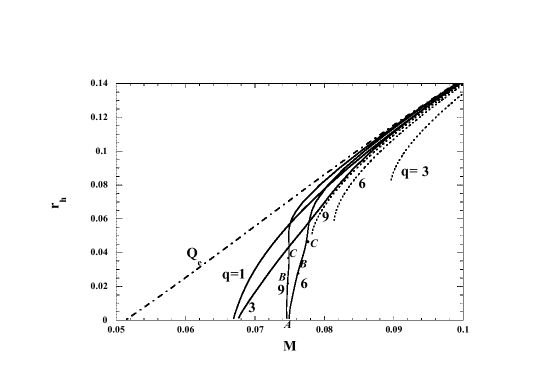
(a)

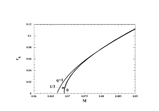
(b)

FIG. 12.: $M$-$r_{h}$ diagram of the dyon solutions with $\sqrt{Q_{m}^{2}+Q_{e}^{2}}=0.1$ and $b=30$. We plot the solutions $q\geq 1$ in (a) and $q\leq 1$ in (b). We can find that though the solutions with small $q$ approach the magnetically charged case (i.e., $q\to 0$), those with large $q$ do not approach the electrically charged case (i.e., $q\to\infty$) because of nontrivial distribution of the axion field. We also plot the dyon solutions in the EMD system by dotted lines in (a).

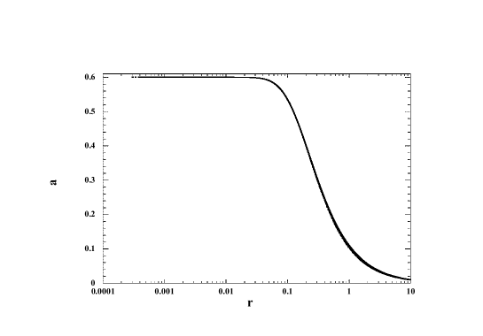
FIG. 13.: The field distributions $r$-$a(r)$ for $b=30$ and $q=0.6$ in numbers of dyon solutions for $3\times 10^{-4}\leq r_{h}\leq 5\times 10^{-3}$. They are almost indistinguishable, which means that the distribution of the axion field is almost independent of the horizon radius.

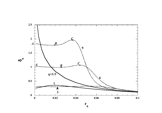
FIG. 14.: $r_{h}$-$\delta_{h}$ relation for the dyon solutions with $b=30$. Though $\delta_{h}$ diverges in the $r_{h}\to 0$ limit for $q=1/3$, it does not for other cases. For other values of $q$, we can find that $\delta_{h}$ decreases as $r_{h}$ decreases, but it eventually increases in the $r_{h}\to 0$ limit because of the large contribution from the axion field.

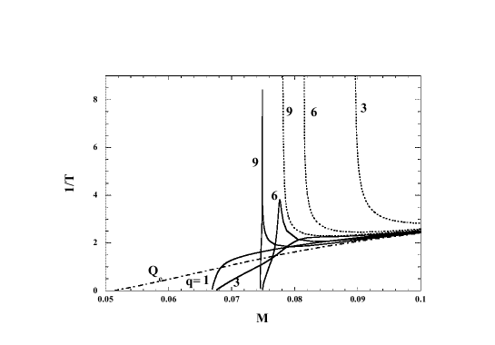
(a)

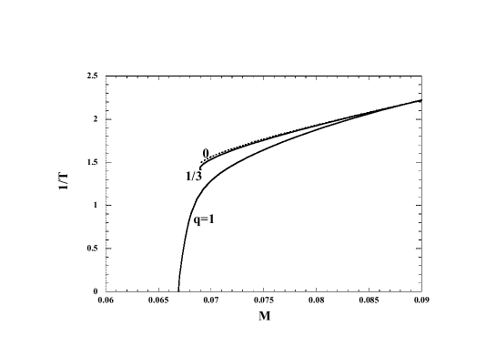
(b)

FIG. 15.: $M$-$1/T$ diagram with the same parameters in Fig. 12. We can find that the temperature diverges for $q\geq 1$ which can be interpreted in the asymptotic analysis. For large $q$, though the temperature approaches zero once, it does not have zero limit in the $r_{h}\to 0$ but diverges in this limit. On the contrary, the dyon solutions in the EMD system have an extreme limit where the temperature becomes zero.

VI Discussion

We investigate the static spherically symmetric solutions in the EBIDA system. When the solutions do not have both electric and magnetic charge, there is no contribution from the axion field. (i) In the electrically charged case, there is neither extreme solution nor particle-like solution, both of which exist in the EBI system. The temperature of the black hole diverges monotonically in the $r_{h}\to 0$ limit. The dilaton charge $\Sigma$ becomes larger than the gravitational mass $M$ in this limit. (ii) In the magnetically charged case, the extreme solution exists when $\alpha_{m}=1/2$ and particle-like solutions exist when $\alpha_{m}<1/2$. For $\alpha_{m}>1/2$, the solution in the $r_{h}\to 0$ limit corresponds to naked singularity. The temperature of the black hole remains finite in the $r_{h}\to 0$ limit for $\alpha_{m}\geq 1/2$, while it diverges for $\alpha_{m}<1/2$. There is no BPS saturated solution. (iii) In the dyon case, we can obtain a nontrivial axion field. Contributions of the axion field mainly depend on the ratio $q=Q_{e}/Q_{m}$. Since $a_{h}$ is restricted to $a_{h}<q$, solutions in the $q\to 0$ limit approach the corresponding magnetically charged solutions. But they do not approach the electrically charged ones in the $q\to\infty$ limit. As for the temperature, whether or not it diverges in the $r_{h}\to 0$ is only determined by $\alpha_{m}$. We can show that there is no inner horizon in any charged case, and the global structure is the Schwarzschild type.

Here, we discuss some outstanding issues. First, we compare our results with those in Ref. [27] where a slightly different system from ours was considered. What they call the soliton corresponds to our “particle-like” solution considered in the electrically charged case. We required the finiteness of the dilaton field for a particle-like solution and find such a solution in the magnetically charged case. They did not investigate the dyon case. However, since the extended version of the EBIDA model has a SL(2,R) duality, it is easy to produce the dyon solutions. Those solutions will have distinct properties from us.

Second, we comment on the stability of solutions and the relation between the inverse string tension $\alpha^{\prime}$ and the gravitational constant $G$. We considered them in our previous paper on the monopole case[24]. By using catastrophe theory[31, 32], we find that the discussion is irrelevant even if we include the dyon case. This implies that our solutions are stable against spherical perturbations. As we discussed following Ref. [25], we identify the supersymmetric spin $0$, $1/2$ particle with the extreme solution. For the dyon case, the extreme solution is realized for $b=25(1+q^{2})$ when we fixed the charge $\sqrt{Q_{e}^{2}+Q_{m}^{2}}=0.1$. We can find in Fig. 12 that the result is not affected from the monopole case. We find $2\pi\alpha\sim 1.73G$ for the dyonic DEBIon black hole.

Finally, we denote future work. Though we find the particle-like solution in the magnetically charged case, it is unsatisfactory as a candidate of the remnant of the Hawking radiation for the following reasons. (i) Since it appears in the $r_{h}\to 0$ limit where the Hawking temperature diverges, the quantum effect of the gravity may affect the results. (ii) Since the particle-like solution admits a conical singularity at the origin, there still appears naked singularity. These results may be modified if the higher curvature terms are taken into account. As was already pointed out, it is difficult to obtain the counterpart of the BI action in the gravity part. It is open to question whether or not the singularity inside the horizon is regulated as the electric field is in the BI action. Concerning this, BI type action for gravity was considered in Ref. [33] and the regular black hole solution was obtained, though there is no theoretical background at present. But considering higher curvature such as the Gauss-Bonnet term is still important, since if the black hole solution is not singular in this case, there may be a possibility that this result is preserved even if we consider the higher curvature term. This type of consideration may shed light on the realization of the dream in Ref. [34].

REFERENCES

- [1] M. Born and L. Infeld, Proc. Roy. Soc. A 144, 425, (1934).
- [2] E. Fradkin and A. Tseytlin, Phys. Lett. B 163, 123 (1985); A. Tseytlin, Nucl. Phys. B 276, 391 (1986).
- [3] J. Polchinski, hep-th/9611050; M. Aganagic, J. Park, C. Popescu and J. H. Schwarz, Nucl. Phys. B 496, 191 (1997); A. Tseytlin. Nucl. Phys. B 469, 51 (1996).
- [4] G. W. Gibbons, Nucl. Phys. B 514, 603 (1998); C. G. Callan, Jr. and J. M. Maldacena, Nucl. Phys. B 513, 198 (1998).
- [5] N. Seiberg and E. Witten, JHEP 9909, 32 (1999).
- [6] D. Mateos, Nucl. Phys. B 577, 139 (2000).
- [7] M. Novello, V. A. De Lorenci, J. M. Salim and R. Klippert, Phys. Rev. D 61, 045001 (2000).
- [8] G. Boillat, J. Math. Phys. 11, 941 (1970).
- [9] G. W. Gibbons and C. A. R. Herdeiro, hep-th/008052.
- [10] A. Tseytlin, Nucl. Phys. B 501, 41 (1997); D. Brecher, Phys. Lett. B 442, (1998); S. Gonorazky, F. Schaposnik and G. Silva, Phys. Lett. B 449, 187 (1999); J. Park, Phys. Lett. B 458, 471 (1999); For a review, see hep-th/9908105 and hep-th/9909154.
- [11] D. V. Gal’tsov and R. Kerner, Phys. Rev. Lett. 84, 5955 (2000).
- [12] V. V. Dyadichev and D. V. Gal’tsov, Nucl. Phys. B 590, 504 (2000); ibid., Phys. Lett. B 486, 431 (2000); M. Wirschins, A. Sood and J. Kunz, hep-th/0004130.
- [13] M. Demianski, Found. Phys. 16, 187 (1986).
- [14] By this term we mean a solution which has conical singularity at the origin and has finite energy.
- [15] H. d’ Oliveira, Class. Quant. Grav. 11, 1469 (1994).
- [16] D. Wiltshire, Phys. Rev. D 38, 2445 (1988).
- [17] H. Salazar, A. García and J. Plebański, J. Math. Phys. 28, 2171 (1987).
- [18] E. Ayón-Beato and A. García, Phys. Rev. Lett. 80, 5056 (1998); ibid., Gen. Rel. Grav. 31, 629 (1999); ibid., Phys. Lett. B 464, 25 (1999).
- [19] J. Bardeen, in Proceedings of GR5, Tiflis, U. S. S. R., 1968; A. Borde, Phys. Rev. D 55, 7615 (1997).
- [20] E. Bergshoeff, E. Sezgin, C. Pope and P. Townsend, Phys. Lett. B 188, 70 (1987); R. Metsaev, M. Rahmanov and A. Tseytlin, Phys. Lett. B 193, 207 (1987); C. Callan, C. Lovelace, C. Nappi and S. Yost, Nucl. Phys. B 308, 221 (1988); O. Andreev and A. Tseytlin, Nucl. Phys. B 311, 205 (1988).
- [21] G. W. Gibbons and K. Maeda, Nucl. Phys. B 298, 741 (1988); D. Garfinkle, G. T. Horowitz and A. Strominger, Phys. Rev. D 43, 3140 (1991).
- [22] B. A. Campbell, N. Kaloper and K. A. Olive, Phys. Lett. B 263, 364 (1991); 285, 199 (1992); K. Lee and E. Weinberg, Phys. Rev. D 44, 3159 (1991).
- [23] A. Shapere, S. Trived and F. Wilczek, Mod. Phys. Lett. A 6, 2677 (1991).
- [24] T. Tamaki and T. Torii, Phys. Rev. D 62, 061501 (2000).
- [25] G. W. Gibbons and D. A. Rasheed, Nucl. Phys. B 454, 185 (1995).
- [26] D. A. Rasheed and G. W. Gibbons, Phys. Lett. B 365, 46 (1996).
- [27] G. Clément and D. V. Gal’tsov, Phys. Rev. D 62, 124013 (2000).
- [28] In this paper, we study the tree-level action. When we are interested in the higher-loop action, the coupling constant takes different value by assuming anomaly cancellation (See. Ref. [20]).
- [29] P. Bizon, Acta. Phys. Pol. B 25, 877 (1994).
- [30] G. Cheng, W. Lin and R. Hsu, J. Math. Phys. 35, 9 (1994).
- [31] R. Thom, Structural Stability and Morphogenesis (Benjamin, New York, 1975).
- [32] K. Maeda, T. Tachizawa, T. Torii and T. Maki, Phys. Rev. Lett. 72, 450 (1994); T. Torii, K. Maeda and T. Tachizawa, Phys. Rev. D 51, 1510 (1995); T. Tachizawa, K. Maeda and T. Torii, ibid., 4054 (1995).
- [33] J. A. Feigenbaum, Phys. Rev. D 58, 124023 (1998).
- [34] A. A. Tseytlin, hep-th/9410008, in Proc. of the Conference on Current Topics in Astrofundamental Physics (1994).