Navigation in Curved Space-Time

Abstract

A covariant and invariant theory of navigation in curved space-time with respect to electromagnetic beacons is written in terms of J. L. Synge’s two-point invariant world function. Explicit equations are given for navigation in space-time in the vicinity of the Earth in Schwarzschild coordinates and in rotating coordinates. The restricted problem of determining an observer’s coordinate time when their spatial position is known is also considered.

I Introduction

Curved space-time forms the basis for most classical theories of gravity, such as general relativity. These theories are usually based on a metric for four dimensional space-time [1]. Some of the basic concepts used in general relativity and related theories are transformation rules for tensors, the affine connection, and the relation of the metric to proper time along an observer’s world line. A useful, but little-used concept, is that of the world function of space-time, as developed by J. L. Synge. The world function is essentially one-half of the squared measure between two points in space-time. The utility of the world function comes from the fact that it is closely related to experiments, and that it is a type of scalar quantity. Since the world function transforms as a kind of scalar, it allows us to formulate geometric quantities in a covariant way. Hence, the world function is a valuable tool for understanding the geometric ideas in metric theories of gravity, in three dimensional differential geometry and tensor analysis, and wherever arbitrary coordinate systems are used. As an example of the utility of the world function, I present its application to the problem of navigation in a curved space-time. This application actually goes beyond a simple pedagogical example because it deals with the real-world need for precise navigation and time dissemination.

Consider the problem of an observer who wants to navigate in a curved space-time with respect to electromagnetic beacons. I use the word navigate to mean that the observer determines his or her coordinate position and coordinate time along their world line, in some system of space-time coordinates. I assume that the electromagnetic beacons continuously broadcast their space-time coordinates and that this information is imbedded in the emitted electromagnetic signals. Furthermore, I assume that an observer at unknown coordinates $(t_{o},{\bf x}_{o})$ simultaneously receives these signals from four beacons. The observer’s navigation problem is to compute his position $(t_{o},{\bf x}_{o})$ from the four received emission event coordinates $(t_{s},{\bf x}_{s})$, $s=$1,2,3,4, of the electromagnetic beacons.

In the case of flat space-time, the observer must solve the four simultaneous equations

$$|{\bf x}_{o}-{\bf x}_{s}|^{2}-c^{2}(t_{o}-t_{s})^{2}=0,\;\;\;\;s=1,...4$$ (1)

Equation (1) contains four invariant statements: light signals travel ‘on the light cone’ from each emission event to the observer, (see Figure 1). To resolve the branches of the light cones, the causality conditions $t_{o}>t_{s}$, for $s=$1,$\dots$4, must be added. The relations in Eq. (1) are the basic navigation equations applied by users of satellite navigation systems, such as the U.S. Global Positioning System (GPS) and the Russion Global Navigation Satellite System (GLONASS) [2, 3, 4]. The coordinates of the four events, $(t_{s},{\bf x}_{s})$, correspond to particular radio emissions by the satellites. The emission event coordinates can be extracted from information transmitted by digital codes.

Equation (1) is commonly used in two different ways. First, an observer may receive radio signals from satellites and compute his or her space-time coordinates $(t_{o},{\bf x}_{o})$ in terms of four known satellite emission events $(t_{s},{\bf x}_{s})$. The second use of Eq. (1) is to locate a satellite, which is at an unknown position $(t_{o},{\bf x}_{o})$ in terms of four ground observations at known coordinates $(t_{s},{\bf x}_{s})$. For this use, we apply the causality condition $t_{s}>t_{o}$, $s=$1,$\dots$4. In Eq. (1), the assumption is made that space-time is flat and the speed of light $c$ is constant. Furthermore, by using Eq. (1) we make the geometric optics approximation that the wavelength of the electromagnetic waves is small compared to all physical dimensions of the receiver and transmitter systems [5, 6].

In recent years, there have been significant improvements in the stability of frequency standards and measurement techniques [7, 8]. Consequently, over satellite-to-ground distances, precise measurements should be interpreted within the framework of a curved space-time theory [9, 10, 11, 12]. Furthermore, the equations for navigation in space-time should be manifestly covariant and also invariant [13].

In this work, I write down a generalization of the navigation Eq. (1) for curved space-time and give the detailed equations that must be solved for navigating in the vicinity of the Earth, both in Schwarzschild coordinates and in rotating coordinates. I still retain the geometric optics approximation, however, I take into account deviations from flatness to first order in the metric. This means that the flat-space light cones in Eq. (1) are replaced by equations for null geodesics. The required navigation equations are simply expressible in terms of the world function developed by J. L. Synge [14]. The resulting formalism takes into account the delay of electromagnetic signals due to the presence of a gravitational field. The detailed equations have application to a user who wants to accurately compute his coordinate position and time. In general, the world function approach is useful in applications where high-accuracy measurements must be made over large distances. An application of recent interest is the design of space-based interferometers for precision sensing and surveillance purposes [15, 16]. In some of these designs, in order to achieve high-resolution imaging long base lines (hundreds of kilometers) must be used between Earth satellites and their separations may need to be accurate to within a micrometer or better. To unambiguously and accurately define such positions, a curved space-time approach should be used that takes into account the warping of the geometry of space-time due to gravitational effects.

In section II, I write the generalization of Eq. (1) in terms of the world function and point out the limitations of navigation in curved space-time by electromagnetic beacons. In section III, I briefly describe the restricted problem of computing an observer’s coordinate time if his or her spatial coordinates are known (a restricted type of navigation). In sections IV and V, I give the detailed equations applicable to navigation in the vicinity of the Earth in Schwarzschild coordinates and in coordinates that rotate with the Earth.

II Navigation Equations

The world function was initially introduced into tensor calculus by Ruse [17, 18], Synge [19], Yano and Muto [20], and Schouten [21]. It was further developed and extensively used by Synge in applications to problems dealing with measurement theory in general relativity [14]. In general, the world function has received little attention, so I give the following definition. Consider two points, $P_{1}$ and $P_{2}$, in a general space-time, connected by a unique geodesic path $\Gamma$ given by $x^{i}(u)$, where $u_{1}\leq u\leq u_{2}$. A geodesic is defined by a class of special parameters $u^{\prime}$ that are related to one another by linear transformations $u^{\prime}=au+b$, where $a$ and $b$ are constants. Here, $u$ is a particular parameter from the class of special parameters that define the geodesic $\Gamma$, and $x^{i}(u)$ satisfy the geodesic equations

$$\frac{d^{2}x^{i}}{du^{2}}+\Gamma^{i}_{jk}\frac{dx^{j}}{du}\frac{dx^{k}}{du}=0$$ (2)

The world function between $P_{1}$ and $P_{2}$ is defined as the integral along $\Gamma$

$$\Omega(P_{1},P_{2})=\frac{1}{2}(u_{2}-u_{1})\int^{u_{2}}_{u_{1}}\,g_{ij}\frac{dx^{i}}{du}\frac{dx^{j}}{du}\,du$$ (3)

The value of the world function has a geometric meaning: it is one-half the square of the space-time distance between points $P_{1}$ and $P_{2}$. Its value depends only on the eight coordinates of the points $P_{1}$ and $P_{2}$. The value of the world function in Eq. (3) is independent of the particular special parameter $u$ in the sense that under a transformation from one special parameter $u$ to another, $u^{\prime}$, given by $u=au^{\prime}+b$, with $x^{i}(u)=x^{i}(u(u^{\prime}))$, the world function definition in Eq. (3) has the same form (with $u$ replaced by $u^{\prime}$).

The world function is a two-point invariant in the sense that it is invariant under independent transformation of coordinates at $P_{1}$ and at $P_{2}$. Consequently, the world function characterizes the space-time. For a given space-time, the world function between points $P_{1}$ and $P_{2}$ has the same value independent of the metric-induced coordinates. A simple example of the world function is for Minkowski space-time, which is given by

$$\Omega(x^{i}_{1},x^{j}_{2})=\frac{1}{2}\,\eta_{ij}\,\Delta x^{i}\,\Delta x^{j}$$ (4)

where $\eta_{ij}$ is the Minkowski metric with only non-zero diagonal components $(-1,+1,+1,+1)$, and $\Delta x^{i}=(x_{2}^{i}-x_{1}^{i})$, $i=0,1,2,3$, where $x_{1}^{i}$ and $x_{2}^{i}$ are the coordinates of points $P_{1}$ and $P_{2}$, respectively. Up to a sign, the world function gives one-half the square of the geometric measure in space-time. Calculations of the world function for specific space-times can be found in Refs. [14, 22, 23, 24] and application to Fermi coordinates in Synge[14] and Gambi et al. [25].

The generalization to a curved space-time of the navigation Eq. (1) is given by

$$\Omega(x^{i}_{s},x^{j}_{o})=0,\;\;\;\;s=1,2,3,4$$ (5)

where $x^{i}_{s}=(t_{s},{\bf x}_{s})$ are the coordinates of the emission events, $x^{i}_{o}=(t_{o},{\bf x}_{o})$ are the observer coordinates and the world function is defined by Eq. (3). Within the geometric optics approximation, Eq. (5) forms a natural generalization of the navigation Eq. (1). In addition to Eq. (5), the appropriate causality conditions $t_{s}>t_{o}$ or $t_{o}>t_{s}$, for $s=$1,$\dots$4, must be added. The set of relations in Eq. (5) are manifestly covariant and invariant due to the transformation properties of the world function under independent space-time coordinate transformations at point $P_{1}$ and at $P_{2}$.

From the definition of the world function, the intrinsic limitations of navigation in a curved space-time are evident: the world function $\Omega(P_{1},P_{2})$ must be a single-valued function of $P_{1}$ and $P_{2}$. In general, if two or more geodesics connect the points $P_{1}$ and $P_{2}$, then $\Omega(P_{1},P_{2})$ will not be single-valued and the set of equations in Eq. (5) may have multiple solutions or no solutions. Such conjugate points $P_{1}$ and $P_{2}$ are known to occur in applications to planetary orbits and in optics [14]. However, when the points $P_{1}$ and $P_{2}$ are close together in space and in time and the curvature of space-time is small, we expect the world function to be single valued and the solution of Eq. (5) to be unique. Therefore, navigation in curved space-time is limited by the possibility of determining a set of four unique null geodesics connecting four emission events to one reception event. In the case of strong gravitational fields as may exist in the vicinity of a black hole, or when the (satellite) radio beacons are at large distances from the observer in a space-time of small curvature, navigation by radio beacons may not be possible in principle. In such cases, one may have to supplement radio navigation by inertial techniques; see, for example, the discussion by Sedov [26].

III Coordinate Time at a Known Spatial Position

Consider the restricted problem of an observer that knows his spatial position and wants to obtain his coordinate time [27]. A null geodesic connects the emission and reception events, so the value of the world function is zero,

$$\Omega(t_{s},{\bf x}_{s},t_{o},{\bf x}_{o})=0$$ (6)

where the satellite emission event coordinates $(t_{s},{\bf x}_{s})$ and the observer spatial coordinates ${\bf x}_{o}$ are known. Equation (6) must be supplemented by the causality condition $t_{o}>t_{s}$. The observer obtains his coordinate time by solving Eq. (6) for $t_{o}$.

As a simple example of the application of Equation (6), consider an observer at a known spatial location who wants to compute his coordinate time in flat space-time in a rotating system of coordinates, $y^{i}$, by receiving signals from a satellite at $P_{s}=(t_{s},{\bf y}_{s})$. I take the transformation from Minkowski coordinates $x^{i}$ to rotating coordinates $y^{i}$ to be given by

$$y^{0} = x^{0}$$ (7)

$$y^{1} = \cos(\frac{\omega}{c}x^{0})\,x^{1}-\sin(\frac{\omega}{c}x^{0})\,x^{2}$$ (8)

$$y^{2} = \sin(\frac{\omega}{c}x^{0})\,x^{1}+\cos(\frac{\omega}{c}x^{0})\,x^{2}$$ (9)

$$y^{3} = x^{3}$$ (10)

The world function is a two-point invariant that characterizes the space-time, so, in the rotating coordinates its value does not change. Using the world function for Minkowski space-time in Eq. (4) and the transformation to rotating coordinates $y^{i}$ in Eq. (10), the world function is given by

$$\Omega(P_{s},P_{o}) = \Omega(t_{s},{\bf x}_{s},t_{o},{\bf x}_{o})=\bar{\Omega}(t_{s},{\bf y}_{s},t_{o},{\bf y}_{o})$$ (11)

$$= \frac{1}{2}\left[({\bf y}_{o}-{\bf y}_{s})^{2}-c^{2}(t_{o}-t_{s})^{2}\right]$$ (13)

$$+({\bf y}_{s}\times{\bf y}_{o})\cdot{\bf n}\,\sin(\omega(t_{o}-t_{s}))+2\left[{\bf y}_{s}\cdot{\bf y}_{o}-({\bf y}_{s}\cdot{\bf n})({\bf y}_{o}\cdot{\bf n})\right]\sin^{2}(\frac{1}{2}\omega(t_{o}-t_{s}))$$

where ${\bf n}$ is a unit vector in the direction of the angular velocity vector ${\bf\omega}$, which I take to be along the z-axis. I assume that the angular velocity of rotation is small, so that the time for light to travel from a satellite at ${\bf y}_{s}$ to an observer at ${\bf y}_{o}$ is small compared to the period of rotation $2\pi/\omega$. I define the small dimensionless parameter $\delta=\omega|{\bf y}_{o}-{\bf y}_{s}|/c<<1$. Equation (6) can then be solved for $\Delta t=t_{o}-t_{s}$ by iteration, leading to

$$c\Delta t = |{\bf y}_{o}-{\bf y}_{s}|+\frac{1}{c}({\bf y}_{s}\times{\bf y}_{o})\cdot{\bf\omega}$$ (15)

$$+\frac{1}{2c^{2}}|{\bf y}_{o}-{\bf y}_{s}|\left\{\frac{\left[({\bf y}_{s}\times{\bf y}_{o})\cdot{\bf\omega}\right]^{2}}{|{\bf y}_{o}-{\bf y}_{s}|^{2}}+\left[\omega^{2}{\bf y}_{s}\cdot{\bf y}_{o}-({\bf y}_{s}\cdot{\bf\omega})({\bf y}_{o}\cdot{\bf\omega})\right]\right\}+O(\delta^{4})$$

The first term on the right side of Eq. (15) divided by $c$ is the time for light to travel from the emission event at the satellite, $(t_{s},{\bf y}_{s})$, to the observer at event, $(t_{o},{\bf y}_{o})$, in the absence of rotation. The second term is the celebrated Sagnac effect [28, 29, 30, 31], which depends on the sense of rotation of the coordinates (sign of ${\bf\omega}$). The third term is a higher order correction that is independent of the sense of rotation; i.e., it is the same when ${\bf\omega}\rightarrow-{\bf\omega}$. This term is on the order of 5$\times$10^-14 s for satellite and Earth angular velocity of rotation parameters appropriate to the GPS. Equation (15) leads to the standard expression for the Sagnac effect when we take the difference of propagation times for clockwise ($\Delta T_{-}$) and counterclockwise ($\Delta T+$) propagation of light along the limit of a sequence of tangents on the perimeter of a circle, $\Delta T_{+}-\Delta T_{-}=4{\bf A}\cdot\omega/c^{2}$, where ${\bf A}$ is the included area[28, 29, 30, 31]. Note that the third term in Eq. (15) does not contribute to the difference of round-trip times, $\Delta T_{+}-\Delta T_{-}$, so it is not measurable in a Sagnac experiment. However, this term does contribute to a determination of coordinate time.

IV Navigation in the Vicinity of the Earth

In the vicinity of the Earth, the gravitational potential can be approximated by [32]

$$\phi(r,\theta)=-\frac{GM}{r}\left[1-J_{2}\left(\frac{R_{e}}{r}\right)^{2}P_{2}(\cos(\theta))\right]$$ (16)

where $P_{2}(x)=(3x^{2}-1)/2$ is the second Legendre polynomial and $J_{2}$ is the Earth’s quadrupole moment, whose value is approximately $J_{2}=1.0\times 10^{-3}$. However, for navigation in the vicinity of the Earth, we can neglect $J_{2}$ since it is three orders of magnitude smaller than the dimensionless coefficient of the monopole potential $GM/r$, which already contributes small corrections to propagation of electromagnetic radiation. I also neglect the effects of the rotation of the Earth, which give rise to small terms in the metric of space-time $g_{0\alpha}$, since these effects are completely negligible at the present time [31]. Therefore, the Earth’s gravitational field can be sufficiently accurately described using the Schwarzschild metric [33]

$$-ds^{2}=-\left(1-\frac{2GM}{c^{2}r}\right)c^{2}dt^{2}+\frac{dr^{2}}{1-\frac{2GM}{c^{2}r}}+r^{2}(d\theta^{2}+\sin^{2}\theta d\phi^{2})$$ (17)

In Eq. (17), I neglect the gravitational field of the sun and other planets, since the Earth is in free fall and these fields are essentially (up to tidal terms) cancelled as a result of the equivalence principle.

Using the transformation to rectangular coordinates

$$x^{0} = ct$$ (18)

$$x^{1} = r\sin\theta\cos\phi$$ (19)

$$x^{2} = r\sin\theta\sin\phi$$ (20)

$$x^{3} = r\cos\theta$$ (21)

and expanding in the small parameter $GM/c^{2}r$, the metric for the Schwarzschild space-time can be written to first order as a sum of the Minkowski metric, $\eta_{ij}$, and the deviation from flatness tensor $h_{ij}$ as

$$-ds^{2}=g_{ij}\,dx^{i}dx^{j}=\left(\eta_{ij}+h_{ij}\right)dx^{i}dx^{j}$$ (22)

where $h_{ij}$ is given by

$$h_{ij}dx^{i}dx^{j}=\frac{2GM}{c^{2}}\left[\frac{(cdt)^{2}}{r}+\frac{(x^{\alpha}\,dx^{\alpha})^{2}}{r^{3}}\right]$$ (23)

The assumption that $GM/c^{2}r\ll 1$ is a restriction on the region of validity of Eq. (22) to large $r$ compared with the gravitational radius of the Earth, which is $2GM/c^{2}\approx 0.88$cm.

Following Synge, I approximate the world function for the metric in Eq. (22) by replacing the integrals over the geodesic $\Gamma$ by integrals along a straight line, and taking the special parameter $u$ to vary in the range $0\leq u\leq 1$, which leads to [14]

$$\Omega(x^{i}_{1},x^{j}_{2})=\frac{1}{2}\,\eta_{ij}\,\Delta x^{i}\,\Delta x^{j}+\frac{1}{2}\Delta x^{i}\,\Delta x^{j}\int_{0}^{1}h_{ij}du$$ (24)

I find that explicit evaluation of these integrals (see Appendix B) leads to [34]

$$\Omega(x^{i}_{1},x^{j}_{2}) = \frac{1}{2}\eta_{ij}\Delta x^{i}\Delta x^{j}+\frac{GM}{c^{2}}\,\left[|{\bf x}_{2}-{\bf x}_{1}|+\frac{c^{2}\Delta t^{2}}{|{\bf x}_{2}-{\bf x}_{1}|}\right]\;\log\left(\frac{\tan(\frac{\theta_{1}}{2})}{\tan(\frac{\theta_{2}}{2})}\right)$$ (26)

$$+\frac{GM}{c^{2}}|{\bf x}_{2}-{\bf x}_{1}|\left(\cos\theta_{1}-\cos\theta_{2}\right)$$

where $c\Delta t=x^{0}_{2}-x^{0}_{1}$, and $\theta_{1}$ and $\theta_{2}$ are defined by

$$\cos\theta_{a}=\frac{{\bf x}_{a}\cdot({\bf x}_{2}-{\bf x}_{1})}{|{\bf x}_{a}||{\bf x}_{2}-{\bf x}_{1}|},\;\;\;\;a=1,2$$ (27)

See Appendix C for an estimate of the error in Eq. (26). The first term on the right side of Eq. (26) is the world function for Minkowski space-time, given in Eq. (4). The second and third terms in Eq. (26) give the corrections to the world function of Minkowski space-time due to the gravitational effects of mass $M$. The expression in Eq. (26) can be used in Eq. (5) as a basis for navigation, or in Eq. (6) for computing coordinate time in the vicinity of the Earth.

As an example of using the world function in Eq. (26), I consider determining the coordinate time of an observer at a known spatial position ${\bf x}_{o}$ in the vicinity of Earth, using standard Schwarzschild coordinates. Taking the satellite position as ${\bf x}_{s}={\bf x}_{1}$, the observer position ${\bf x}_{o}={\bf x}_{2}$, and making use of the small parameter $GM/(c^{2}|{\bf x}_{o}-{\bf x}_{s}|)\ll 1$, I solve Eq. (6) by iteration, leading to

$$c\,\Delta t=|{\bf x}_{o}-{\bf x}_{s}|+\frac{GM}{c^{2}}\left[2\log\left(\frac{\tan(\frac{\theta_{s}}{2})}{\tan(\frac{\theta_{o}}{2})}\right)+\cos\theta_{s}-\cos\theta_{o}\right]$$ (28)

The first term in Eq. (28) divided by $c$ is the time for light to propagate from ${\bf x}_{s}$ to ${\bf x}_{o}$. The second term is the small correction due to the presence of the Earth’s mass $M$ distorting the space-time in its vicinity. This expression takes into account the delay of the electromagnetic signal in a gravitational field (see, for example, Ref. [35, 1, 36] and references cited therein). For a satellite directly overhead, where ${\bf x}_{o}$ and ${\bf x}_{s}$ are co-linear with the origin of coordinates, Eq. (28) leads to the result

$$c\,\Delta t=|{\bf x}_{o}-{\bf x}_{s}|+\frac{2GM}{c^{2}}\log\frac{|{\bf x}_{s}|}{|{\bf x}_{o}|}$$ (29)

Equation Eq. (29) is obtained by considering the spatial geometry shown in Figure 2. Define a triangle by the three points: origin at $O$, satellite at $P_{s}$ with coordinates ${\bf x}_{s}$, and observer at $P_{o}$ with coordinates ${\bf x}_{o}$. From point $P_{o}$, draw a line $\overline{P_{o}M}$ perpendicular to $\overline{OP}_{s}$ and define its length to be $h$. Equation (29) is obtained from Eq. (28) by setting $\theta_{s}=\theta_{1}$, $\theta_{o}=\theta_{2}$, ${\bf x}_{s}={\bf x}_{1}$, and ${\bf x}_{o}={\bf x}_{2}$, using the definitions in Eq. (27) and the relations

$$\cos\theta_{s} = -1+\frac{1}{2}\,\left(\frac{h}{l_{1}}\right)^{2}$$ (30)

$$\cos\theta_{o} = -1+h^{2}\,\left(\frac{1}{l_{1}l_{2}}+\frac{1}{2l_{1}^{2}}+\frac{1}{2l_{2}^{2}}\right)$$ (31)

where

$$l_{1} = \left({\bf x}_{s}-{\bf x}_{o}\right)\cdot\frac{{\bf x}_{s}}{|{\bf x}_{s}|}$$ (32)

$$l_{2} = \frac{{\bf x}_{o}\cdot{\bf x}_{s}}{|{\bf x}_{s}|}$$ (33)

$$l_{2}^{2} = |{\bf x}_{o}|^{\,2}-h^{2}$$ (34)

and taking the limit as $h\rightarrow 0$. Note that Eq. (28) and (29) are expressed in terms of Schwarzschild spatial coordinates (and do not contain the temporal coordinates) of satellite ${\bf x}_{s}$ and observer ${\bf x}_{o}$, because the Schwarzschild space-time is static; i.e., the space-time admits a hypersurface orthogonal time-like Killing vector field [37].

V Navigation in the Vicinity of the Earth in Rotating Coordinates

In practical navigation problems, an observer or user of a satellite navigation system is often interested in their space-time position with respect to the Earth–which defines a rotating coordinate system. To compute an observer space-time position in a rotating system of coordinates, I apply the navigation Eq. (5) in the rotating system. Having computed the world function for Schwarzschild space-time in Eq. (26) in a ‘nonrotating’ system of coordinates $x^{i}$, the invariant nature of the world function can be used to write the world function in a rotating system of coordinates, $y^{i}$, using the transformation in Eq. (10):

$$\Omega(x^{i}_{1},x^{j}_{2}) = \tilde{\Omega}(t_{1},{\bf y}_{1},t_{2},{\bf y}_{2})$$ (35)

$$= \frac{1}{2}\eta_{ij}\,y^{i}y^{j}+\Delta F$$ (38)

$$+\frac{GM}{c^{2}}\frac{1}{\left[({\bf y}_{2}-{\bf y}_{1})^{2}+2\Delta F\right]^{1/2}}\left[({\bf y}_{2}-{\bf y}_{1})^{2}+(c\,\Delta t)^{2}+2\,\Delta F\right]\,\log\left(\frac{F_{2}}{F_{1}}\right)$$

$$-\frac{GM}{c^{2}}(|{\bf y}_{1}|+|{\bf y}_{2}|)+\frac{GM}{c^{2}}\left(\frac{1}{|{\bf y}_{1}|}+\frac{1}{|{\bf y}_{2}|}\right)\left[{\bf y}_{1}\cdot{\bf y}_{2}-\Delta F\right]$$

where

$$\Delta F = ({\bf y}_{1}\times{\bf y}_{2})\cdot{\bf n}\,\sin(\omega\Delta t)+2\left[{\bf y}_{1}\cdot{\bf y}_{2}-({\bf y}_{1}\cdot{\bf n})({\bf y}_{2}\cdot{\bf n})\right]\sin^{2}\left(\frac{\omega\Delta t}{2}\right)$$ (39)

$$F_{1} = {\bf y}_{1}\cdot({\bf y}_{2}-{\bf y}_{1})-\Delta F+|{\bf y}_{1}|\,\left[({\bf y}_{2}-{\bf y}_{1})^{2}+2\,\Delta F\right]^{1/2}$$ (40)

$$F_{2} = {\bf y}_{2}\cdot({\bf y}_{2}-{\bf y}_{1})+\Delta F+|{\bf y}_{2}|\,\left[({\bf y}_{2}-{\bf y}_{1})^{2}+2\,\Delta F\right]^{1/2}$$ (41)

For navigation in the vicinity of the Earth in rotating coordinates, the observer must solve the four simultaneous Eqs. (5) using the world function in Eq. (38). In general, this must be done numerically.

Consider the simpler problem of determining an observer’s coordinate time at a known spatial location. Analytic results can be obtained in this case. I solve Eq. (6) for $\Delta t=t_{o}-t_{s}$ using the world function in Eq. (38) by defining three small dimensionless parameters, $x=\omega\Delta t$, $\delta=\omega|{\bf y}_{o}-{\bf y}_{s}|/c$, and $\alpha=GM\omega/c^{3}$, and solving for $x$ as a function of $\delta$ by iteration. This leads to

$$c\Delta t = |{\bf y}_{o}-{\bf y}_{s}|+\frac{1}{c}({\bf y}_{s}\times{\bf y}_{o})\cdot{\bf\omega}+\frac{1}{2c^{2}}|{\bf y}_{o}-{\bf y}_{s}|\left\{\frac{\left[({\bf y}_{s}\times{\bf y}_{o})\cdot{\bf\omega}\right]^{2}}{|{\bf y}_{o}-{\bf y}_{s}|^{2}}+\omega^{2}{\bf y}_{s}\cdot{\bf y}_{o}-({\bf y}_{s}\cdot{\bf\omega})({\bf y}_{o}\cdot{\bf\omega})\right\}$$ (43)

$$+\frac{GM}{c^{2}}\left[2+\frac{1}{c}\frac{({\bf y}_{s}\times{\bf y}_{o})\cdot{\bf\omega}}{|{\bf y}_{o}-{\bf y}_{s}|}\right]\log\left(\frac{\tan(\frac{\theta_{o}}{2})}{\tan(\frac{\theta_{s}}{2})}\right)+\frac{GM}{c^{2}}\left[1+\frac{1}{c}\frac{({\bf y}_{s}\times{\bf y}_{o})\cdot{\bf\omega}}{|{\bf y}_{o}-{\bf y}_{s}|}\right]\left(\cos\theta_{s}-\cos\theta_{o}\right)$$

In Eq. (43), I have dropped small terms of $O(\alpha\delta)$, $O(\alpha^{2})$, and $O(\delta^{4})$. Equation (43) gives the coordinate time for the signal to travel from the source to the observer, $\Delta t=t_{o}-t_{s}$. Since the propagation time $\Delta t$ is given in a rotating system of coordinates, Eq. (43) contains the Sagnac effect, modified by the presence of mass M (the Earth). The first term corresponds to the propagation of the electromagnetic signal from the satellite at ${\bf y}_{s}$ to observer at ${\bf y}_{o}$ in (flat, nonrotating) Minkowski space-time coordinates. The second term is the standard Sagnac correction term (expressed in terms of coordinate time) that depends on the sense of rotation ${\bf\omega}$, which appeared in rotating coordinates in vacuum (see Eq. (15)). The third term on the right side of Eq. (43) also appears in flat space-time and, as previously mentioned, it does not depend on the sense of the rotation; it is the same when $\omega\rightarrow-\omega$ and, hence, does not contribute to the Sagnac effect. The last two terms on the right-hand side of Eq. (43) are corrections to the coordinate time of propagation due to the Earth’s mass $M$. Note that the coefficients of each of the last two terms also depend on $\omega$. This represents a modification of the Sagnac effect due to the presence of mass $M$.

The rotation of the coordinate system leads to a break in spherical three-dimensional symmetry. Note that terms two and three on the right side of Eq. (43), which are due to the rotation, have a cylindrical symmetry determined by the direction of ${\bf\omega}$, as expected. On the other hand, the last two terms that depend on the mass $M$ have coefficients that have a constant (spherically symmetric) term plus a term that depends on the sense of rotation (linear in $\omega$).

VI Conclusion

If an observer simultaneously receives electromagnetic signals from four electromagnetic beacons in flat space-time, he or she can compute their position in space-time by solving the four light cone Eqs. (1). This procedure is routinely carried out everyday by users of satellite navigation systems such as GPS and GLONASS. Equation (1) neglects small effects of gravitational fields on electromagnetic signal propagation. In this work, I have included these effects in a natural way using the two-point invariant world function developed by J. L. Synge. I have given a simple covariant and invariant formulation of the navigation problem in Eq. (5). An approximation to the world function in Schwarzschild coordinates is given in Eq. (26), and in coordinates that rotate with the Earth in Eq. (38). In the future, approximations to the world function may be obtained for the case of the Eddington and Clark metric [38] and Eqs. (1) may serve as the basis for high-accuracy navigation throughout our solar system.

I have implicitly used the geometric optics approximation by assuming that electromagnetic radiation propagates along null geodesics. Furthermore, when navigating inside the Earth’s atmosphere, or when radiation traverses the atmosphere, there is an additional signal delay that is bigger than the effects discussed here and must be taken into account in detail. I have neglected these effects. Consequently, the results here are valid for observers in orbit around the Earth outside the Earth’s atmosphere. Work is in progress to extend the world function approach to simultaneously include gravitational and index-of-refraction (atmospheric) effects.

The world function approach used here can be applied to areas that require precise definitions of distances over satellite-to-ground length scales. A particular application area of recent interest, where high-accuracy position is required over hundreds of kilometers, is flying satellites in formation, for precise sensing and surveillance applications. The high-accuracies needed in definition of satellite positions may require a curved space-time theoretical framework that includes gravitational corrections to flat Minkowski space-time.

A Conventions and Notation

Where not explicitly stated otherwise, I use the convention that Roman indices, such as on space-time coordinates $x^{i}$ take the values $i=0,1,2,3$ and Greek indices take values $\alpha=1,2,3$. Summation is implied over the range of the index when the same index appears in a lower and upper position. In some cases, such as Eq. (23), Greek indices summation is implied when both indices are in the upper position, such as in $x^{\alpha}dx^{\alpha}$.

If $x^{i}$ and $x^{i}+dx^{i}$ are two events along the world line of an ideal clock, then the square of the proper time interval between these events is $d\tau=ds/c$, where the measure $ds$ is given in terms of the space-time metric as $ds^{2}=-g_{ij}\,dx^{i}\,dx^{j}$. I choose $g_{ij}$ to have the signature $+$2. When $g_{ij}$ is diagonalized at any given space-time point, the elements can take the form of the Minkowski metric given by $\eta_{00}=-1$, $\eta_{\alpha\beta}=\delta_{\alpha\beta}$, and $\eta_{0\alpha}=0$.

B Integrals

Two integrals are needed to explicitly evaluate the world function in Eq. (24) (see Ref. [34]):

$$\int_{0}^{1}\frac{1}{r}\,du=\frac{1}{|{\bf x}_{1}-{\bf x}_{2}|}\log\left(\frac{\tan(\frac{\theta_{1}}{2})}{\tan(\frac{\theta_{2}}{2})}\right)$$ (B1)

$$\Delta x^{\alpha}\,\Delta x^{\beta}\int_{0}^{1}\frac{x^{\alpha}\,x^{\beta}}{r^{3}}\,du=|{\bf x}_{1}-{\bf x}_{2}|\,\left[\log\left(\frac{\tan(\frac{\theta_{1}}{2})}{\tan(\frac{\theta_{2}}{2})}\right)+\cos(\theta_{1})-\cos(\theta_{2})\right]$$ (B2)

where $\theta_{1}$ and $\theta_{2}$ are defined in Eq. (27).

C Error in Approximation of the World Function

In Eq. (26), I use Synge’s approximation to the world function for the metric in Eq. (22), which entails replacing the integrals over the geodesic $\Gamma$ by integrals along a straight line L

$$\Omega(P_{1},P_{2})=\frac{1}{2}(u_{2}-u_{1})\int_{\Gamma}\,g_{ij}\frac{dx^{i}}{du}\frac{dx^{j}}{du}\,du\approx\frac{1}{2}(u_{2}-u_{1})\int_{L}\,g_{ij}\frac{dx^{i}}{du}\frac{dx^{j}}{du}\,du$$ (C1)

I take the straight line L to be given by

$$x^{i}_{L}(u)=k(u_{2}-u)x^{i}_{1}+k(u-u_{1})x^{i}_{2}$$ (C2)

where $u_{1}\leq u\leq u_{2}$ and $k=(u_{2}-u_{1})^{-1}$. The error made in this approximation can be computed as follows. Consider two points, $P_{1}$ and $P_{2}$, connected by a family of curves $x^{i}(u,v)$, where $u$ and $v$ are independent parameters. I assume that $P_{1}=x^{i}(u_{1},v)$ and $P_{2}=x^{i}(u_{2},v)$, for all $v$. It is convenient to define the two vector fields

$$U^{i}=\frac{\partial x^{i}}{\partial u},\;\;\;\;\;\;\;\;V^{i}=\frac{\partial x^{i}}{\partial v}$$ (C3)

Note that by construction $V^{i}(u_{1},v)=V^{i}(u_{2},v)=0$. Furthermore, assume that a unique geodesic $\Gamma$ connects the points $P_{1}$ and $P_{2}$, and that this geodesic $\Gamma$ is given by the curve with a particular value of $v=v_{o}$, namely $x^{i}(u,v_{o})$ for $u_{1}\leq u\leq u_{2}$. Define the integral

$$I(v)=\frac{1}{2}(u_{2}-u_{1})\int_{u_{1}}^{u_{2}}\,g_{ij}U^{i}U^{j}\,du$$ (C4)

Now, assume that we have a space-time of small curvature and expand the integral $I(v)$ about the geodesic $\Gamma$

$$I(v)=\Omega(P_{1},P_{2})+\frac{dI(v_{o})}{dv}(v-v_{o})+\frac{1}{2}\frac{d^{2}I(v_{o})}{dv^{2}}(v-v_{o})^{2}+\cdots$$ (C5)

The second term, $dI(v_{o})/dv$, vanishes since this is the definition of a geodesic curve. The error in replacing the integral over a geodesic by an integral over a nearby curve can then be estimated by the third term on the right side of Eq. (C5). Using the relations

$$\frac{\delta V^{i}}{\delta u}=\frac{\delta U^{i}}{\delta v}$$ (C6)

and

$$\frac{\delta U^{i}\;(u,v_{o})}{\delta u}=0$$ (C7)

I find the approximate error is given by

$$I(v)-\Omega(P_{1},P_{2}) \approx \frac{1}{2}\frac{d^{2}I(v_{o})}{dv^{2}}(v-v_{o})^{2}$$ (C8)

$$= \frac{1}{2}(u_{2}-u_{1})(v-v_{o})^{2}\;\int_{u_{1}}^{u_{2}}\left[g_{ij}\frac{\delta U^{i}}{\delta v}\frac{\delta U^{j}}{\delta v}+R_{abcd}V^{a}U^{b}U^{c}V^{d}\right]_{v=v_{o}}\;du$$ (C9)

where the Riemann tensor is given by

$$R^{i}_{jkm}=\Gamma^{i}_{jm,k}-\Gamma^{i}_{jk,m}+\Gamma^{a}_{jm}\Gamma^{i}_{ak}-\Gamma^{a}_{jk}\Gamma^{i}_{am}$$ (C10)

the affine connection is

$$\Gamma^{i}_{jk}=\frac{1}{2}g^{il}\left(g_{jl,k}+g_{kl,j}-g_{jk,l}\right)$$ (C11)

and ordinary partial derivatives with respect to the coordinates are indicated by commas. In Eq. (C9), I have dropped terms of order $O(v-v_{o})^{3}$.

To estimate the error incurred in Eq. (24) by approximating the world function integral over a geodesic by an integral over the straight line in Eq. (C2), I construct an explicit parametrization of curves connecting $P_{1}$ and $P_{2}$:

$$x^{i}(u,v)=\frac{v_{o}-v}{v_{o}}x^{i}_{L}(u)+\frac{v}{v_{o}}x^{i}_{\Gamma}(u)$$ (C12)

where $x^{i}_{L}(u)$ is given by Eq. (C2) and $x^{i}_{\Gamma}(u)$ is a geodesic connecting the points $P_{1}$ and $P_{2}$. For simplicity, in Eq. (C12) I am assuming that the parameter $u=0$ at $P_{1}$ and $u=u_{2}$ at $P_{2}$. For the geodesic connecting the points $P_{1}$ and $P_{2}$, I use a series solution of Eq. (2)

$$x^{i}_{\Gamma}(u)=x_{1}^{i}+\left(\xi^{i}+\frac{1}{2}\Gamma^{i}_{jk}(P_{1})\xi^{j}\xi^{k}\right)\frac{u}{u_{2}}-\frac{1}{2}\Gamma^{i}_{jk}(P_{1})\xi^{j}\xi^{k}\left(\frac{u}{u_{2}}\right)^{2}+\cdots$$ (C13)

where $\xi^{i}=x^{i}_{2}-x^{i}_{1}$. Using the curve parametrization in Eq. (C12), and carrying out the required calculations, I find an estimate of the error in approximating the world function integral by a straight line, given by Eq. (C9), to be

$$I(v)-\Omega(P_{1},P_{2})\approx\frac{1}{24}\left(\frac{v-v_{o}}{v_{o}}\right)^{2}\eta_{ij}\,\Gamma^{i}_{ab}(P_{1})\,\Gamma^{j}_{cd}(P_{1})\,\xi^{a}\xi^{b}\xi^{c}\xi^{d}+O(3)$$ (C14)

where third order terms have been dropped, and $\Gamma^{i}_{ab}(P_{1})$ is the connection evaluated at $P_{1}$. I have taken $\gamma_{ab,c}$ and $\gamma_{ab,cd}$ to be of $O(1)$.

D Note on Iterative Solution of Navigation Equations

Equation (5) is a set of four nonlinear algebraic equations for the four coordinates $(t_{o},{\bf x}_{o})$. A simple method of solution can be applied by linearizing and solving the system by iteration. Setting $x_{o}^{j}=x_{o}^{j}(n)+\delta x^{j}(n)$ in Eq. (5) and expansion to first order in $\delta\,x^{j}(n)$ gives a linear set of equations for $\delta x^{k}(n)$

$$M^{(n)}_{ak}\,\delta x^{k}(n)=-\Omega(x^{i}_{a},x^{j}_{o}(n))=0,\;\;\;\;a=1,2,3,4$$ (D1)

where $\delta x^{k}(n)$ is the correction to the n^th trial value $x^{j}_{o}(n)$ and

$$M^{(n)}_{ak}=\left[\frac{\partial\Omega(x^{i}_{a},x^{j}_{o})}{\partial x^{j}_{o}}\right]_{x^{j}_{o}=x^{j}_{o}(n)}$$ (D2)

I start the iteration by making an ansatz $x^{j}_{o}(1)$ for user coordinates $x^{j}_{o}$, and solve Eqs. (D1) for the first correction, $\delta x^{k}(1)$. The improved solution is then taken to be $x^{j}_{o}(2)=x^{j}_{o}(1)+\delta x^{k}(1)$ and substituted back into Eq. (D1). Iteration is continued until sufficiently small corrections $\delta x^{k}(n)$ are computed.

=6.0cm

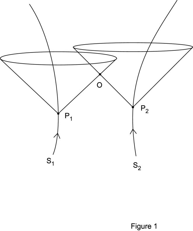
FIG. 1.: Space-time diagram showing two (of the four) satellites with world lines $S_{1}$ and $S_{2}$. Electromagnetic signals are emitted at $P_{1}$ and $P_{2}$, and reach the observer at $O$.

=6.0cm

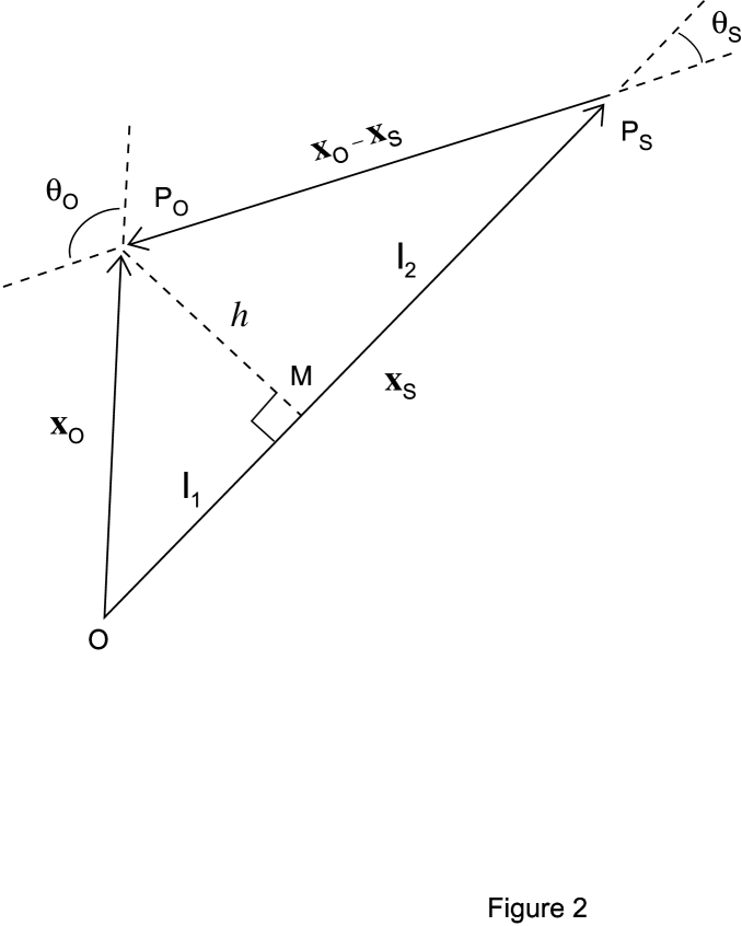
FIG. 2.: The spatial geometry of satellite at $P_{S}$ and receiver at $P_{O}$, with coordinates ${\bf x}_{s}$ and ${\bf x}_{o}$, respectively, showing the angles $\theta_{s}$ and $\theta_{o}$.

REFERENCES

- [1] See, for example, C. M. Will, Theory and Experiment in Gravitational Physics (Cambridge University Press, New York, 1993), revised ed., pp. 67-85.
- [2] B. W. Parkinson and J. J. Spilker, eds., Global Positioning System: Theory and Applications, vol. I and II (P. Zarchan, editor-in-chief), Progress in Astronautics and Aeronautics, vol. 163 and 164 (Amer. Inst. Aero. Astro., Washington, D.C., 1996).
- [3] E. D. Kaplan, Understanding GPS: Principles and Applications, Mobile Communications Series (Artech House, Boston, 1996).
- [4] B. Hofmann-Wellenhof, H. Lichtenegger, and J. Collins, Global Positioning System Theory and Practice (Springer-Verlag, New York, 1993).
- [5] See for example, C. W. Misner, K. S. Thorne, and J. A. Wheeler, Gravitation (W. H. Freeman and Company, New York, 1973), pp. 570-583.
- [6] Yu. A. Kravtsov and Yu. I. Orlov, Geometrical Optics of Inhomogeneous Media (Springer-Verlag, New York, 1990) pp. 3-5.
- [7] G. Petit and P. Wolf, “Relativistic theory for picosecond time transfer in the vicinity of the Earth”, Astron. Astrophys. 286, 971-977 (1994).
- [8] P. Wolf and G. Petit, “Relativistic theory for clock syntonization and the realization of geocentric coordinate times”, Astron. Astrophys. 304, 653-661 (1995).
- [9] B. Guinot, “Application of general relativity to metrology”, Metrologia 34, 261-290 (1997).
- [10] F. de Felice, M. G. Lattanzi, A. Vecchiato, and P. L. Bernacca, “General relativistic satellite astrometry. I. A non-perturbative approach to data reduction”, Astron. Astrophys. 332, 1133-1141 (1998).
- [11] T. B. Bahder, “Fermi Coordinates of an Observer Moving in a Circle in Minkowski Space: Apparent Behavior of Clocks”, Army Research Laboratory, Adelphi, Maryland, U.S.A, Technical Report ARL-TR-2211, May 2000.
- [12] O. J. Sovers, and J. L. Fanselow, “Astrometry and geodesy with radio interferometry: experiments, models, results”, Rev. Mod. Phys. 70, 1393-1454 (1998).
- [13] A. Kheyfets, “Spacetime geodesy”, Weapons Laboratory, Air Force Systems Command, Kirtland Air Force Base, New Mexico, Technical Report No. WL-TN-90-13, July 1991.
- [14] J. L. Synge, Relativity: The General Theory (North-Holland Publishing Co., New York, 1960).
- [15] A. R. Thompson, J. M. Moran, G. W. Swenson, Jr., Interferometry and synthesis in radio astronomy (Krieger Pub. Co., Malabar, Florida, 1994), pp. 138-139.
- [16] P.N.A.M. Visser, “Gravity field determination with GOCE and GRACE”, Adv. Space Res. (UK), Advances in Space Research, 23, 771-776 (1999).
- [17] H. S. Ruse, “Taylor’s Theorem in the Tensor Calculus”, Proc. London Math. Soc. 32, 87-92 (1931).
- [18] H. S. Ruse, “An absolute Partial Differential Calculus”, Quart. J. Math. Oxford Ser. 2, 190 (1931).
- [19] J. L. Synge, “A Characteristic Function in Riemannian Space and its Application to the Solution of geodesic triangles”, Proc. London Math. Soc. 32, 241-258 (1931).
- [20] K. Yano and Y. Muto, “Notes on the deviation of geodesics and the fundamental scalar in a Riemannian space”, Proc. Phys.-Math. Soc. Jap. 18, 142 (1936).
- [21] J. A. Schouten, “Ricci-Calculus. An Introduction to Tensor Analysis and Its Geometrical Applications” (Springer-Verlag, 2nd edition, 1954).
- [22] R. W. John, “Zur Berechnung des geodatischen Abstands und assoziierter Invarianten im relativistischen Gravitationsfeld”, Ann. der Phys. Lpz. 41, 67-80, (1984).
- [23] R. W. John, “The world function of space-time: some explicit exact results for specific metrics”, Ann. der Phys. Lpz. 41, 58-70, (1989).
- [24] H. A. Buchdahl and N. P. Warner, “On the world function of the Schwarzschild field”, Gen. Rel. and Grav. 10, 911-923(1979).
- [25] J. M. Gambi, P. Romero, A. San Miguel, and F. Vicente, “Fermi coordinate transformation under baseline change in relativistic celestial mechanics”, International J. Theor. Phys.30, 1097-1116 (1991).
- [26] L. I. Sedov, “Inertial navigation equations with consideration of relativistic effects”, Sov. Phys. Dokl. 21, 727-729 (1976).
- [27] In the jargon of the timing and time disemination community, determining time at a known location is referred to as “time transfer”.
- [28] G. Sagnac, Compt. Rend. 157, 708, 1410 (1913); J. Phys. Radium, 5th Ser. 4, 177 (1914).
- [29] For a review, see E. J. Post, “Sagnac effect”, Rev. Mod. Phys. 39, 475-493 (1967).
- [30] R. Anderson, H. R. Bilger and G. E. Stedman, “Sagnac” effect: A century of Earth-rotated interferometers”, Am. J. Phys. 62, 975-985 (1994).
- [31] A. Tartaglia, “General relativistic corrections to the Sagnac effect”, Phys. Rev. D 58, 064009/1-7 (1999).
- [32] M. Caputo, The gravity field of the earth (Academic Press, N. Y., 1967).
- [33] See for example, L. D. Landau and E. M. Lifshitz, Classical Theory of Fields (Pergamon Press, New York, Fourth Revised English Edition, 1975).
- [34] There is an error in the tabulation of the second of these integrals in Ref. [14].
- [35] S. Weinberg, Gravitation and Cosmology: Principles and Applications of the Theory of Relativity (John Wiley and Sons, New York, 1972).
- [36] C. M. Will,“The Confrontation between General Relativity and Experiment: A 1998 Update”, Lecture notes from the 1998 Slac Summer Institute on Particle Physics, see gr-qc/9811036.
- [37] For a discussion of space-time symmetry, see for example, R. D’Inverno, Introducing Einstein’s relativity (Oxford University Press, New York, 1995), p.180-183.
- [38] A. Eddington and G. Clark, “The problem of n bodies in general relativity theory”, Proc. Roy. Soc. A 166, 465 (1938).
\epsfsize=6.0cm
\epsfsize=6.0cm