Rotational Instabilities and Centrifugal Hangup

Abstract

One interesting class of gravitational radiation sources includes rapidly rotating astrophysical objects that encounter dynamical instabilities. We have carried out a set of simulations of rotationally induced instabilities in differentially rotating polytropes. An $n$=1.5 polytrope with the Maclaurin rotation law will encounter the $m$=2 bar instability at $T/|W|\gtrsim 0.27$. Our results indicate that the remnant of this instability is a persistent bar-like structure that emits a long-lived gravitational radiation signal. Furthermore, dynamical instability is shown to occur in $n$=3.33 polytropes with the $j$-constant rotation law at $T/|W|\gtrsim 0.14$. In this case, the dominant mode of instability is $m$=1. Such instability may allow a centrifugally-hung core to begin collapsing to neutron star densities on a dynamical timescale. If it occurs in a supermassive star, it may produce gravitational radiation detectable by LISA.

Introduction

One interesting class of gravitational radiation sources includes rapidly rotating astrophysical objects that encounter dynamical instabilities. Linear stability analysis has shown that rapidly rotating bodies may experience global deformations due to the growth of unstable azimuthal modes $e^{\pm im\phi}$ chan69 ; tass78 . The mode numbers $m$ describe the shape of the induced deformation. For example, an $m$=1 mode could result in the development of a one-armed spiral or a simple translation; an $m$=2 mode may produce a bar-shaped distortion; an $m$=3 mode, a triangular distortion; and so on. The onset of such an instability occurs when an object’s ratio of rotational kinetic energy $T$ to gravitational potential energy $W$, $\beta=T/|W|$, exceeds a critical value $\beta_{crit}$.

Both secular and dynamical varieties of these instabilities may exist. A dynamical instability is driven by gravitational and hydrodynamical forces and develops on the order of the rotation period of the system. A secular instability is driven by a dissipative mechanism, such as viscosity or gravitational radiation, and develops on the timescale of that mechanism (which can be many rotation periods). In this paper, we focus on the numerical study of dynamical instabilities, since their development can be followed in a reasonable amount of computational time with explicit hydrodynamical simulations.

There are several types of astrophysical objects that may encounter these rotational instabilities. A star that accretes matter and angular momentum from a binary companion may be spun up to rapid rotation schutz89 . A second example is a centrifugally hung stellar core or “fizzler” thorne96 ; tohl84 ; shli76 . The formation of a fizzler begins when the core of a massive star depletes its nuclear fuel and begins to collapse to neutron star densities. If the core was rotating initially, conservation of angular momentum requires that the core spin up as it collapses. This spin up could actually halt the collapse if the centrifugal force increases to the point where it overcomes the inward gravitational push. The results would be a rapidly rotating, partially collapsed stellar core. Another example is a cooling supermassive star (mass $>10^{6}M_{\sun}$) that also spins up as it contracts nesh00 ; bash99 . Finally, if the merger of a compact binary does not result in an immediate collapse to a black hole, the remnant will be a rapidly rotating compact object lash95 . The nonaxisymmetric deformations induced by rotational instabilities could result in relatively strong gravitational radiation emission from these rapidly rotating objects.

We have performed Newtonian hydrodynamics simulations of dynamical rotational instabilities in two different types of objects cnlb00 ; nct00 . The much studied $m$=2 bar mode is the strongest of the set of global instabilities encountered by an $n$=1.5 polytrope (for which the equation of state gives the pressure $P$ in terms of the density $\rho$ as $P=K\rho^{(1+1/n)}$, where $K$ is the polytropic constant) with the Maclaurin differential rotation law. This instability sets in when $\beta\gtrsim 0.27$. Our results indicate that dynamical instabilities also occur in objects with much lower values of $\beta$. In fact, $n$=3.33 polytropes with the $j$-constant rotation law encounter a dominant $m$=1 instability when $\beta$ reaches $0.14$. Simulations of the bar mode instability and the $m$=1 instability will be discussed in the following sections.

The Bar Mode Instability

There has been a discrepancy in the outcome of previous hydrodynamical simulations of the dynamical bar mode. Namely, simulations carried out by Centrella’s group showed that an object deformed by the bar mode would become axisymmetric again after a short interval shc96 ; hoce94 . This is in contrast to the simulations performed by several other groups, which resulted in bar-shaped final configurations (e.g., new96 ; pick96 ; duri86 ).

The degree of asymmetry in the final configuration is important because an axisymmetric object (rotating about its short symmetry axis) will not emit gravitational radiation. If the simulations performed by Centrella’s groups’s simulations are correct, the instability would produce only a short burst of radiation. However, if the object retains a bar-like structure, as the other simulations seem to indicate, it will go on emitting gravitational radiation, producing a longer-lived signal that would be easier to detect.

This discrepancy is illustrated by the gravitational waveforms shown in Figures 1 and 2. The waveform in Figure 1 is from a simulation performed by Centrella’s group shc96 , with a finite-difference hydrodynamics (FDH) code developed at Drexel University (hereafter called the ${\cal D}$ code). This waveform is burstlike; the amplitude dies off as the object loses its bar-like shape. The waveform in Figure 2 is from a simulation performed by New new96 , with a FDH code developed at Louisiana State University (hereafter called the ${\cal L}$ code). This waveform rings for the duration of the simulation because the object retains its bar-shaped structure.

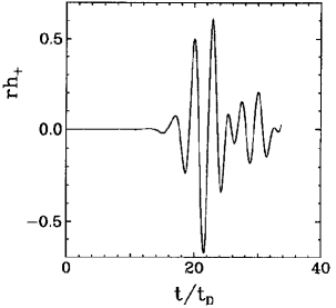
Figure 1: The $h_{+}$ polarization of the gravitational waveform from a ${\cal D}$ code bar mode simulation, as viewed by an observer located along the rotation axis at a distance $r$ from the system. The value $rh_{+}$ has been normalized to $R^{-1}c^{-4}M^{2}G^{2}$; the time is normalized to the dynamical time $t_{D}=[R^{3}/(GM)]^{1/2}$.

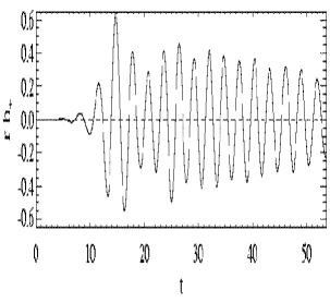
Figure 2: Same as Figure 1, for a simulation performed with the ${\cal L}$ code.

Again, the resolution of this discrepancy is important because if the gravitational radiation signal persists, the total accumulated amplitude could make it easier to detect. The characteristics of New’s waveform are such that if the star’s initial mass and radius are $M=1.4M_{\sun}$ and $R=36\,{\rm km}$, and it is located at a distance of 20 Mpc, the maximum amplitude is $h_{max}\sim 10^{-23}$ and the frequency $f_{gw}$ ranges from $\sim 600-670\,{\rm Hz}$. The scaling is such that $h_{max}\propto R^{-1}$ and $f_{gw}\propto R^{-3/2}$. This signal could possibly be detected with advanced interferometers like LIGO II.

In a recent paper nct00 , we demonstrate that a good deal of progress has been made in resolving the discrepancy among the outcomes of the previous simulations of the bar instability. In an attempt to get at the root of the problem, we examined the differences between the simulations performed with the ${\cal D}$ and ${\cal L}$ codes. One of the main differences is that New’s simulation with the ${\cal L}$ code new96 used a condition called $\pi$-symmetry. The $\pi$-symmetry condition enforces periodic azimuthal symmetry and thus allows the azimuthal resolution to be doubled as the solution only needs to be evolved from $0$ to $\pi$. This symmetry condition does not allow the growth of odd modes in a simulation. However, the use of $\pi$-symmetry in a bar mode simulation seems justified by analytic perturbation anaylsis, which indicates that odd modes will not grow if $\beta<0.32$ toma98 ($\beta$=0.30 in the initial models used by shc96 ; hoce94 ; new96 ).

In order to investigate if the use of $\pi$-symmetry was responsible for differences in the outcomes of the ${\cal D}$ and ${\cal L}$ codes’ bar mode simulations, we reran the ${\cal L}$ code simulation with the $\pi$-symmetry condition turned off (hereafter referred to as simulation ${\cal L}$1). The ${\cal L}$1 simulation started with the same axisymmetric initial model used in the previous simulations shc96 ; new96 . It is constructed in hydrostatic equilibrium with Hachisu’s Self-Consistent Field (SCF) method hach86 . It has an $n$=1.5 polytropic equation of state and is differentially rotating, with an angular momentum distribution identical to that of a Maclaurin spheroid boos73 . It is a highly flattened, rapidly rotating object with $\beta\sim 0.3$ (recall $\beta_{crit}\approx 0.27$).

Equatorial density contours from the last half of the ${\cal L}$1 simulation are shown in Figure 3. As the final frame indicates, the object appears rather symmetric at the end of the run. The resulting waveform (Figure 4) reflects the object’s return to symmetry. This waveform looks much more like the burstlike waveforms of Centrella’s group shc96 ; hoce94 (see, e.g., Figure 1).

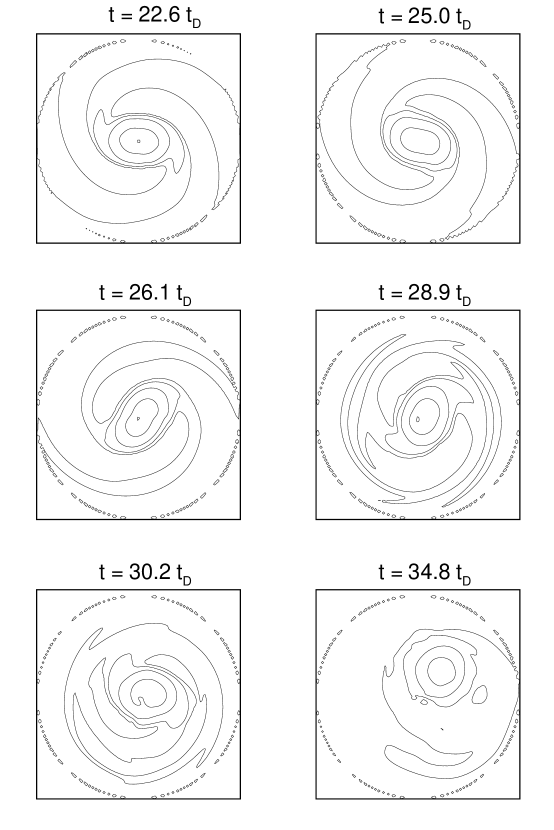
Figure 3: Density contours in the equatorial plane for the later stages of the ${\cal L}$1 simulation are shown. The maximum density has been normalized to unity at $t$=0 and the contour levels are at 0.5, 0.05, 0.005, and 0.0005.

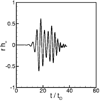
Figure 4: The gravitational waveform from the ${\cal L}$1 simulation is shown. The normalizations are identical to those used in Figure 1.

Thus the ${\cal L}$1 run appears to be in better agreement with the ${\cal D}$ code simulations. But the important question is whether the result on which they agree is the “physical” result. That is, can we with confidence tell the gravitational wave detection community that a star that encounters the bar instability will emit only a burst of radiation?

The answer to that question is no. This is because of an effect that appears late in the ${\cal L}$1 simulation. At about the time that the object loses its bar-like structure, the center of mass of the object moves off the center of the grid. This can be seen in the final frame of Figure 3. In the absence of external forces, the center of mass should not move. This is thus a nonphysical result and must be due to a shortcoming in the numerics of the ${\cal L}$ code.

Before we could say for certain that an axisymmetric configuration is the correct remnant of the bar instability, we needed to find a way to minimize the center of mass motion and see how this affected the outcome of the evolution. Further testing indicated that increasing the radial resolution of the simulation does indeed delay the onset of the motion of the center of mass.

We ran the bar mode simulation with the ${\cal L}$ code once again, this time with double the radial (and axial) resolution used in the ${\cal L}$1 run (this high resolution run will be referred to as ${\cal L}$2). In the ${\cal L}$2 evolution, the bar-like structure is maintained for about 15 more dynamical times (where $t_{D}=(R^{3}/GM)^{1/2}$) than in the ${\cal L}$1 run. The waveform from this run, shown in Figure 6, has a correspondingly longer duration. Doubling the resolution delayed the onset of the center of mass motion, but it did not prevent it. Equatorial density contour plots from the latter portion of the ${\cal L}$2 run are shown in Figure 5. As is evident in the final frame, the bar-like structure (and waveform) decay at the time that the center of mass starts to move.

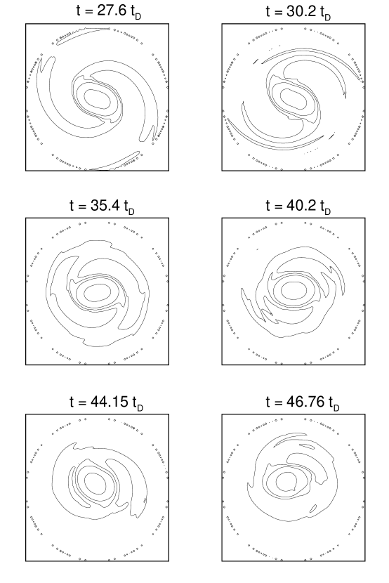
Figure 5: Density contours in the equatorial plane for the later stages of the ${\cal L}$2 simulation are shown. The contour levels are the same as those shown in Figure 3.

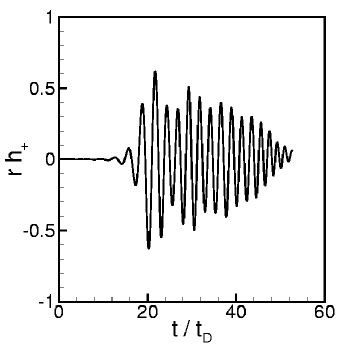
Figure 6: The gravitational waveform from the ${\cal L}$2 simulation is shown. The normalizations are identical to those used in Figure 1.

We have demonstrated that the longer the center of mass motion is suppressed, the longer the bar-like structure is maintained. Since the center of mass motion is unphysical, the decay of the bar is as well. Thus a simulation with very high resolution, or better finite-differencing algorithms that did not develop center of mass motion, should produce a long-lived nonaxisymmetric structure. A recent paper by Brown confirms this brown00 . The FDH PPM hydrocode Brown used to simulate the bar instability explicitly conserves linear momentum, thus preventing center of mass motion from developing. The outcome of Brown’s simulation was indeed a persistent bar.

Recall that this is the outcome of the ${\cal L}$ code’s simulation with $\pi$-symmetry new96 . This symmetry condition prevents the growth of any center of mass motion because it will not allow an $m$=1 mode to grow. Our results and the recent paper by Brown nct00 ; brown00 indicate that the physically accurate outcome of the bar instability in this object is a persistent bar-like configuration that emits gravitational radiation over many cycles and thus may be capable of producing a detectable signal.

Instability at Low $\beta$

We have recently also investigated dynamical rotational instabilities in objects with lower values of $\beta$ cnlb00 . This study was motivated by the fact that centrifugally hung stellar cores, or fizzlers, are likely to have $\beta<0.27$ and thus will not encounter the particular bar mode instability that was discussed in the preceeding section tohl84 ; zwmu97 ; ermu85 .

Previous authors have identified dynamical instabilities in toroidal configurations at values of $\beta\gtrsim 0.1$ wood94 ; toha90 . Thus we decided to investigate the stability properties of spheroidal configurations with off-center density maxima (thinking they may behave more like tori). Our goal was to determine whether spheroidal configurations, representative of fizzlers, could encounter instabilities at lower values of $\beta$.

The initial models for this stability study were constructed with Hachisu’s SCF method. An $n$=3.33 polytropic equation of state was used and is representative of a partially collapsed stellar core. Because we wanted to study models with off-center density maxima, we needed to use a rotation law other than the Maclaurin law. The $j$-constant law does produce off-center density maxima in $n$=3.33 polytropes. The angular velocity distribution $\Omega(\varpi)$ given by this law is

$$\Omega^{2}=\frac{j_{0}^{2}}{(d^{2}+\varpi^{2})^{2}},$$ (1)

where $\varpi$ is the cylindrical radius and $d$ is an arbitrary constant. As $d$ approaches zero, the specific angular momentum approaches the constant $j_{0}$. We constructed models with $d$=0.2. Figure 7 displays meridional density contour plots of four of the equilibrium models we constructed. Off-center density maxima appear as $\beta$ is increased.

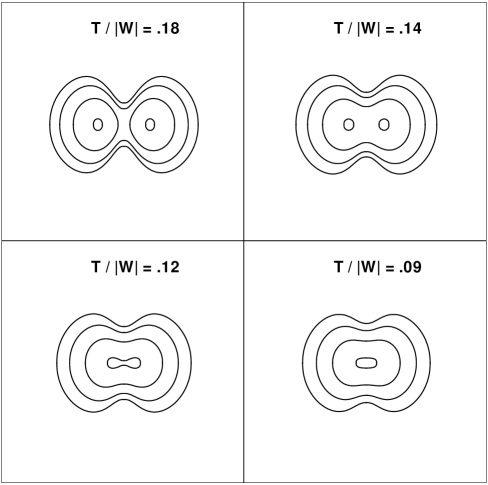
Figure 7: Density contours in the meridional plane are shown for 4 equilibrium models with $d$=0.2 and $n$=3.33. The models are labeled with their values of $\beta=T/|W|$. The initial maximum density has been normalized to unity and the contour levels are at 0.9, 0.1, 0.01, and 0.001.

We performed simulations of these models with the ${\cal L}$ code and with Brown’s PPM hydrocode. The ${\cal L}$ code uses a cylindrical grid and Brown’s code uses a Cartesian grid. We have evolved all four of the models shown in Figure 7. The onset of instability is near $\beta$=0.14. Both the $\beta$=0.14 and 0.18 models are clearly unstable (see below). We have also run simulations of the models with $\beta$=0.12 and $0.09$. The $\beta$=0.12 model was run for about 40 $t_{D}$. At the end of the simulations, the $m$=1 mode was just starting to grow. The $\beta$=0.09 model was run for 35 $t_{D}$ and showed no mode growth. We plan to run longer, higher resolution simulations to determine the value of $\beta$ at which the instability sets in. Note that no significant center of mass motion was seen in these simulations.

The evolution of the model with $\beta$=0.14 exhibits a dynamical instability that is very similar in simulations performed with both codes. The development of the instability is shown in the equatorial density contour plots of Figure 8 (from the ${\cal L}$ code run). The torus pinches off to produce a single high density region, indicative of a $m$=1 mode. This dense region starts to collapse at late times, as is evident from the appearance of higher density contours. Figures 9 and 10 show the amplitude of the modes that grow during the evolutions performed with both codes. The $m$=2, 3, and 4 modes grow in sequence after the $m$=1 mode. The pattern speeds for the $m$=1 and $m$=2 modes are identical. Thus the $m$=2 mode is an harmonic of the $m$=1 mode. The constant amplitude of the $m$=4 mode in Brown’s simulation is a result of the symmetry of his Cartesian grid.

Figure 8: Density contours in the equatorial plane are shown for the model with $\beta$=0.14. The darkness of the shading increases as the density decreases. The contour levels are 0.01, 0.1, 0.9, 2, and 4 times the maximum density at the initial time.

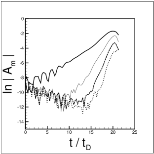
Figure 9: The growth of the amplitudes $|A_{m}|$ for $m$=1 (thick solid line), $m$=2 (thin solid line), $m$=3 (dashed line), and $m$=4 (dotted line) is shown for the ${\cal L}$ code simulation of the $\beta$=0.14 model. These amplitudes were calculated in the equatorial plane for a ring with radius $\varpi$=0.32.

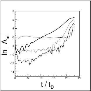
Figure 10: Same as Figure 9, for Brown’s simulation.

The evolutions of the $\beta$=0.18 model also exhibit dynamical instability. The mode amplitude plots from these runs are shown in Figures 11 and 12. The instability grows more quickly in this model than in the $\beta$=0.14 model, as expected. The $m$=1 mode grows at about the same rate in the simulations of both codes. The ${\cal L}$ code run shows the $m$=2, 3, and 4 modes growing in sequence, just like in the $\beta$=0.14 simulation; the $m$=2 mode is again an harmonic of the $m$=1 mode. Brown’s run, however, shows the $m$=1 and $m$=2 modes growing at the same rate. These modes are not harmonics in his simulation. We plan to investigate the differences in these results with higher resolution simulations.

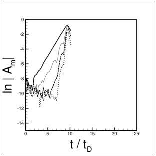
Figure 11: Same as Figure 9, except that the model has $\beta$=0.18.

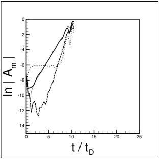
Figure 12: Same as Figure 10, except that the model has $\beta$=0.18.

Our study demonstrates that dynamical instabilities can occur in differentially rotating polytropes with relatively low values of $\beta$. Note that Pickett, Durisen, and Davis pick96 also found a dominant $m$=1 instability in a centrally condensed configuration. The instability in their model set in at $\beta$=0.2. The model had an $n$=1.5 polytropic equation of state and was constructed with the so-called $n^{\prime}$=2 rotation law. This rotation law places more angular momentum in the outer regions of the model than does the $j$-constant law. Their model did not have off-center density maxima.

We plan to carry out more detailed studies to investigate the character of these unstable modes and their properties for various values of the polytropic index $n$ and the rotation law parameter $d$.

If this instability occurs in centrifugally hung stellar cores, collapse to neutron star densities may result. Our simulations do show that the density is increasing at the end of the unstable runs. Further studies are needed to determine how dense the remnant becomes and to see if the $m$=1 mode will result in the star moving with velocities comparable to those of actual neutron stars.

Longer runs on larger grids are needed to obtain the full gravitational radiation waveforms. However, we can estimate the properties of the emission during the initial stages of the development of the instability. For a fizzler that starts out with $M\sim 1.4M_{\odot}$ and $R\sim 200$km, the peak emission will occur at $f_{gw}\sim 200$Hz. The peak amplitude $h_{max}$ will be $\sim 10^{-24}r_{20}^{-1}$ for $\beta=0.14$, and $\sim 10^{-23}r_{20}^{-1}$ for $\beta=0.18$. Here, $r_{20}$ is the distance to the source in units of 20 Mpc. Emission from such unstable cores may be detectable with advanced ground-based interferometers like LIGO II.

An even more optimistic scenario for the detection of gravitational radiation occurs if this type of instability is encountered by a cooling and contracting supermassive star nesh00 ; bash99 . If the star’s ratio $GM/Rc^{2}$ is $\sim 15$ when the instability develops (a value that is approximately appropriate for an uniformly rotating star), $f_{gw}$ will be $\sim 10^{-3}$ Hz and $h_{max}$ will be $\sim 10^{-18}r_{20}^{-1}$ for $\beta=0.14$ and $\sim 10^{-17}r_{20}^{-1}$ for $\beta=0.18$. Such signals would be easily detectable by the space-based LISA detector.

References

- (1) Chandrasekhar, S., Ellipsoidal Figures of Equilibrium, Yale University Press, New Haven, 1969.
- (2) Tassoul, J., Theory of Rotating Stars, Princeton University Press, Princeton, 1978.
- (3) Schutz, B., Class. Quantum Gravity 6, 1761 (1989).
- (4) Thorne, K., in Proceedings of the Snowmass 95 Summer Study on Particle and Nuclear Astrophysics and Cosmology, edited by E. W. Colb and R. Peccei, World Scientific, Singapore, 1996.
- (5) Tohline, J. E., Astrophys. J. 285, 721 (1984).
- (6) Shapiro, S. and Lightman, A., Astrophys. J. 207 263 (1976).
- (7) New, K. C. B. and Shapiro, S. L., Astrophys. J., in press (2000) (astro-ph/0010574).
- (8) Baumgarte, T. and Shapiro, S. L., Astrophys. J. 526, 941 (1999).
- (9) Lai, D. and Shapiro, S. L., Astrophys. J. 442, 259 (1995).
- (10) Centrella, J. M., New, K. C. B., Lowe, L. L., and Brown, D., Astrophys. J. Lett, submitted (2000).
- (11) New, K. C. B., Centrella, J. M., and Tohline, J. E., Phys. Rev. D 62, 064019 (2000).
- (12) Smith, S., Houser, J., and Centrella, J., Astrophys. J. 458, 236 (1996).
- (13) Houser, J. and Centrella, J., Phys. Rev. D 54, 7278 (1994).
- (14) New, K. C. B., Ph.D. Thesis, Louisiana State University (1996).
- (15) Pickett, B., Durisen, R., and Davis G., Astrophys. J. 458, 714 (1996).
- (16) Durisen, R. Gingold, R., Tohline, J., and Boss, A., Astrophys. J. 305, 281 (1986).
- (17) Toman, J., Imamura, J. N., Pickett, B. K., and Durisen, R. H., Astrophys. J. 497, 370 (1998).
- (18) Hachisu, I., Astrophys. J. Suppl. 61, 479 (1986).
- (19) Bodenheimer, P. and Ostriker, J., Astrophys. J. 180, 159 (1973).
- (20) Brown, J. D., Phys. Rev. D, in press (2000) (gr-qc/0004002).
- (21) Zwerger, T. & Müller, E., Astronomy & Astrophysics 320, 209 (1997).
- (22) Eriguchi, Y. & Müller, E., Astronomy & Astrophysics 147, 161 (1985).
- (23) Woodward, J., Tohline, J., & Hachisu, I., Astrophys. J. 420, 247 (1994).
- (24) Tohline, J. & Hachisu, I. 1990, Astrophys. J. 361, 394 (1990).