Initial condition of a gravitating thick loop cosmic string and linear perturbations

The initial data of the gravitational field produced by a loop thick string is considered. We show that a thick loop is not a geodesic on the initial hypersurface, while a loop conical singularity is. This suggests that there is the “critical thickness” of a string, at which the linear perturbation theory with a flat space background fails to describe the gravity of a loop cosmic string. Using the above initial data, we also show that the linear perturbation around flat space is plausible if the string thickness is larger than $\sim 5\times 10^{-3}a$, where $a$ is the curvature radius of the loop.

I Introduction

For the past few decades, gravity of cosmic strings and gravitational waves from them have been investigated by many researchers[1]–[11]. There are two physical contexts to investigate gravity of cosmic strings. One is the cosmological context and another is in the technical problem in general relativity: the treatment of concentrated line sources.

In the cosmological context, cosmic strings are topological defects associated with the symmetry breaking in unified theories[1]. In the simplest case, the dynamics of cosmic strings is governed by the Nambu-Goto action. If the self-gravity of strings is ignored (test string case), the Nambu-Goto action admits oscillatory solutions. It is considered that these oscillations lead the emission of gravitational waves and strings gradually lose their kinetic energy by this emission[2]. Further, relic gravitational waves emitted by cosmic strings might be detectable by the gravitational wave detectors to be constructed in the near future[3]. Though this is a quite fascinating prediction, it is not clear whether or not it can be taken seriously. Recently, by taking into account the self-gravity of the Nambu-Goto string, it is shown that the oscillatory behavior of a self-gravitating string coupled to gravitational wave is quite different from that of a test string[4]. The dynamical degree of freedom concerning the perturbative oscillations of an infinite string is completely determined by that of gravitational waves and a self-gravitating infinite string does not oscillate spontaneously unlike an infinite test string.

To give a completely precise dynamics of gravitating cosmic strings, we must solve the Einstein equations and the evolution equations of the Higgs and gauge fields from generic initial data, which is impossible at present. So it will be instructive to replace a cosmic string by a concentrated line source and clarify its gravity at first[5]. However, it is known that the mathematical description of a self-gravitating thin string is delicate because the support of a string is a surface of co-dimension two. In general relativity, there is no simple prescription of an arbitrary concentrated line source where the metric becomes singular[6].

In spite of these difficulties, a conical singularity, which appears in some exact solutions to the Einstein equations, is often regarded as a self-gravitating cosmic string. (For example, see Ref.[7].) This is one of the idealizations of the concentrated matter sources. Since a spacetime containing a straight gauge string has the asymptotically conical structure[8], this idealization seems plausible when the string thickness is much smaller than the other physical scale of interests.

As an extension of this idealization, one might expect that an oscillating cosmic string can be also idealized by an oscillating conical singularity. However, as pointed out by Unruh et al.[9], the worldsheet of a conical singularity is totally geodesic. This behavior is also seen in the time symmetric initial data of gravity of a loop conical singularity[10] and similar results are also obtained in Refs.[4, 11]. The dynamics of conical singularities is completely determined without their equations of motion. This geodesic property of a conical singularity shows that the idealization of cosmic strings by conical singularities might gives the different dynamics from that of cosmic strings in the early universe which have their finite thickness. Further, this implies that the dynamics of cosmic strings is not idealized by that of conical singularities, though it seems natural to expect that loops of cosmic string can be regarded as conical singularities when the loop radius is much larger than the string thickness.

In this paper, we reconsider the above geodesic property pointed out in Ref.[9] using a time symmetric initial data containing a thick loop string. We show that the zero thickness of strings is essential to this geodesic property. Because of the singular metric, gravity near the loop conical singularity is so strong that the loop itself is a geodesic on the initial surface. On the other hand, the core of the thick loop string is not a geodesic on the initial surface and the curvature of a test loop on a flat space is naturally reproduced in the limit $G\rightarrow 0$ where $G$ is Newton’s gravitational constant. Then, the geodesic property in Ref.[9] should not be taken seriously when we consider the dynamics of cosmic strings, since cosmic strings in the early universe have their own finite thickness. This also implies that we must take into account the effect of the string thickness when we discuss the dynamics of cosmic strings.

This behavior of the gravity of a thick string loop also suggests that there is a criterion in the string thickness at which the linear perturbation theory around a flat background spacetime fails to describe the gravity of cosmic strings. We call this thickness “critical thickness” and evaluate this criterion in this paper. The geodesic property in Ref.[9] does not depend on the loop radius and its deficit angle. When the spacetime contains a sufficiently small loop conical singularity, this loop is a geodesic on this spacetime and the other geodesics on this spacetime are quite different from those on the flat spacetime, on which geodesics are straight lines. On the other hand, gravity of a thick loop string is not so strong as mentioned above. This suggests that the linear gravity is plausible if the string is sufficiently thick. Then, for a fixed loop radius and a fixed deficit angle, there exists a critical thickness and the linear gravity on a flat background spacetime is valid if the string thickness is much greater than this critical thickness.

To discuss the initial data of the gravity of a thick string loop and evaluate the above critical thickness, we first construct an example of the initial data in which the matter concentrates on the torus shell. Since the gravity of a cosmic string has asymptotically conical structure, we use the initial data derived by Frolov et al.[10] as a solution outside the torus. Using this example, we explicitly show that the core of the loop string is not a geodesic if the string has its finite thickness, while the loop approaches to a geodesic in the zero-thickness limit. Though the matter distribution in this example is too artificial as a realistic cosmic string loop, our conclusion is also true even if the matter distribution is smooth. Our example also shows that the initial data derived by Frolov et al.[10] may be regarded as the gravitational field produced by a smooth matter distribution. So, using this initial data as the geometry outside the matter field, we derive the above critical thickness of a string by comparing with a linear solution on the flat space background.

This paper is organized as follows: In Sec.II, we briefly review the ADM initial constraints and the treatment of the $\delta$-function distribution of the matter field on the initial surface to construct an example of the gravitational field produced by a loop matter distribution. In Sec.III, we construct an initial data of a thick loop string and discuss whether the string is a geodesic on the initial surface or not. We discuss the above critical thickness in Sec.IV. The final section (Sec.V) is devoted to summary and discussions.

Throughout this paper we work in relativistic units, so that the speed of light is equal to unity.

II Initial value constraints and Junction conditions

In 4-dimensional spacetime $({\cal M},g_{ab})$, we consider a zero extrinsic curvature 3-dimensional spacelike submanifold $(\Sigma,q_{ab})$. We denote the unit normal vector of $\Sigma$ in ${\cal M}$ by $u^{a}$. The induced metric $q_{ab}$ on $\Sigma$ from the metric $g_{ab}$ on ${\cal M}$ is given by $q_{ab}:=g_{ab}+u_{a}u_{b}$. The zero extrinsic curvature means the spacetime is momentarily static at $(\Sigma,q_{ab})$. The ADM initial-value constraints for a momentarily static hypersurface $(\Sigma,q_{ab})$ are reduced to[12]

$${}^{(3)}\!R=16\pi GT_{\perp\perp},$$ (1)

where ${}^{(3)}\!R$ is the Ricci scalar curvature of $\Sigma$ and $T_{\perp\perp}:=T_{ab}u^{a}u^{b}$ is the energy density of the matter field on the hypersurface $\Sigma$. In terms of a conformally transformed metric $\tilde{q}_{ab}:=\phi^{-4}q_{ab}$, the constraint (1) is given by

$$\tilde{D}^{a}\tilde{D}_{a}\phi-\frac{1}{8}\phi{}^{(3)}\!\tilde{R}=-2\pi G\phi^{5}T_{\perp\perp},$$ (2)

where $\tilde{D}_{a}$ and ${}^{(3)}\!\tilde{R}$ are the covariant derivative and the scalar curvature associated with the metric $\tilde{q}_{ab}$, respectively. In this paper, we concentrate only on the geometry of $\Sigma$ using the constraint (2) (or (1)).

For simplicity, we consider $\delta$-function distribution of matter energy density at the 2-dimensional hypersurface ${\cal S}$ on $\Sigma$ to construct an example of solutions to Eq.(2). To treat $\delta$-function distribution of the matter energy, we apply Israel’s condition[13] on the initial surface, which is derived from the constraint (2). To derive this condition, we first divide $(\Sigma,q_{ab})$ into two manifolds $(\Sigma_{\pm},q_{ab\pm})$ with the boundaries $\partial\Sigma_{\pm}$ and then identify ${\cal S}=\partial\Sigma_{+}=\partial\Sigma_{-}$. This identification implies $n_{a+}=n_{b-}$, where $n_{a\pm}$ are the unit normal vector of $\partial\Sigma_{\pm}$ on $\Sigma_{\pm}$, respectively. The induced metrics $h_{ab\pm}$ on $\partial\Sigma_{\pm}$ from $q_{ab\pm}$ are given by $h_{ab\pm}:=q_{ab\pm}-n_{a\pm}n_{b\pm}$, respectively. Since $\partial\Sigma_{\pm}$ are diffeomorphic to each other, $h_{ab\pm}$ satisfy the condition

$$h_{ab+}=h_{ab-}.$$ (3)

By virtue of the constraint (1), the $\delta$-function distribution of the matter energy density also gives the gap of the extrinsic curvatures $\kappa_{ab\pm}$ of $\partial\Sigma_{\pm}$ facing to $\Sigma_{\pm}$. $\kappa_{ab\pm}$ are defined by $\kappa_{ab\pm}:=-(h_{a}^{\;\;c}h_{b}^{\;\;d}D_{c}n_{d})_{\pm}$, where $D_{a}$ is the covariant derivative associated with the metric $q_{ab}$. Introducing the Gaussian normal coordinate $\chi$ in the neighborhood of ${\cal S}$ by $n_{a\pm}=(d\chi)_{a}$, the scalar curvature ${}^{(3)}\!R$ on $\Sigma$ is decomposed as follows:

$${}^{(3)}\!R={}^{(2)}\!R-(\kappa^{\;\;a}_{a})^{2}+\kappa_{a}^{\;\;b}\kappa_{b}^{\;\;a}+2\frac{\partial}{\partial\chi}\kappa_{a}^{\;\;a}.$$ (4)

When $T_{\perp\perp}$ is given by

$$T_{\perp\perp}=\mu\delta(\chi),$$ (5)

the integration of (1) over the infinitesimal interval of $\chi$ yields

$$\kappa_{a+}^{\;\;a}-\kappa_{a-}^{\;\;a}=8\pi G\mu.$$ (6)

Hence all conditions for the identification ${\cal S}=\partial\Sigma_{\pm}$ on the momentarily static initial data are (3) and (6).

III Initial condition of a thick loop string

Here, we consider a momentarily static initial data of gravity produced by a thick loop string. In this paper, we assume that the vacuum region outside the loop is given by the initial data for a loop conical singularity derived by Frolov et al.[10] as mentioned in the Introduction (Sec.I). In this section, we first review the conformally flat version of the initial data for a loop conical singularity in Ref.[10]. Second, replacing the conical singularity by a matter distribution, we construct an example of a gravitating thick loop string. Then we discuss whether the loop is a geodesic on the initial surface or not. Though we concentrate only on a conformally flat initial data, the similar behavior is also seen in the conformally non-flat version. (See Appendix A.)

A Initial condition of a loop conical singularity

To discuss the initial condition for a loop conical singularity, we introduce the toroidal coordinate system. First, we consider the flat space metric

$$ds^{2}_{E}=d\rho^{2}+dz^{2}+\rho^{2}d\varphi^{2}.$$ (7)

Defining the functions $\sigma$ and $\psi_{*}$ by

$$\rho=a\frac{\sinh\sigma}{N^{2}},\quad z=a\frac{\sin\psi_{*}}{N^{2}},\quad N(\sigma,\psi_{*}):=\sqrt{\cosh\sigma-\cos\psi_{*}},$$ (8)

where $0\leq\sigma\leq\infty$ and $-\pi\leq\psi_{*}\leq\pi$, the line element (7) becomes

$$ds^{2}_{E}=\frac{1}{N^{4}}ds^{2}_{*}:=\frac{a^{2}}{N^{4}}\left(d\sigma^{2}+d\psi_{*}^{2}+\sinh^{2}\sigma d\varphi^{2}\right).$$ (9)

The geometrical meaning of the coordinates $\sigma$ and $\psi_{*}$ is depicted in Fig.1. A $\sigma$=constant surface is a torus with circular cross sections of radius $a\mbox{csch}\sigma$; the central axis of the tube forms a circle of radius $\rho=a\coth\sigma$ in the plane $z=0$. The ring $\rho=a$, $z=0$ is the limit torus $\sigma=\infty$.

To construct the initial data of a loop conical singularity at the limit torus $\sigma=\infty$, we remove a pair of spherical caps spanning the loop as shown in Fig.2[10]. First, we fix an arbitrary angular deficit $2\pi\alpha<2\pi$. We restrict $\psi_{*}$ to the range $-\pi(1-\alpha)<\psi_{*}<\pi(1-\alpha)$, identify these end points of this interval. Applying a conformal factor $(\phi N)^{4}$ to Eq.(9), the physical line element associated with the metric $q_{ab}$ is given by

$$ds^{2}=(\phi N)^{4}ds^{2}_{E}=\phi^{4}ds^{2}_{*}.$$ (10)

Second, we rescale the coordinate $\psi_{*}$ by

$$\psi:=\eta\psi_{*},\quad-\pi\leq\psi\leq\pi,\quad\eta:=\frac{1}{1-\alpha}.$$ (11)

Then the conformally transformed metric $\tilde{q}_{ab}$ is given by

$$\tilde{q}_{ab}=a^{2}\left((d\sigma)_{a}(d\sigma)_{b}+\frac{1}{\eta^{2}}(d\psi)_{a}(d\psi)_{b}+\sinh^{2}\sigma(d\varphi)_{a}(d\varphi)_{b}\right).$$ (12)

Though the exposed spherical faces have the same intrinsic geometry, their extrinsic curvatures have opposite sign in $(\Sigma,N^{-4}\tilde{q}_{ab})$. This discontinuity disappears in $(\Sigma,q_{ab})$ if the conformal factor $\phi(\sigma,\psi)$ satisfies the following boundary conditions:

1. $\phi(\sigma,\psi)$ is even in the inversion $\psi\rightarrow-\psi$ and smooth at $\psi=\pm\pi$;

2. $\phi N\rightarrow 1$ at $\sigma\rightarrow\infty$;

3. $\phi N\rightarrow$ constant at $\sigma\rightarrow 0$.

By virtue of the condition (i), the extrinsic curvature of the surface $\psi=\pm\pi$ in $(\Sigma,q_{ab})$ vanishes and no discontinuity is there. The condition (ii) guarantees that $(\Sigma,q_{ab})$ has the conical structure with the deficit angle $\alpha$ at the limit tours $\sigma=\infty$. $(\Sigma,q_{ab})$ is asymptotically flat by virtue of the final condition (iii).

Assuming $\varphi^{a}:=(\partial/\partial\varphi)^{a}$ is a Killing vector on $(\Sigma,q_{ab})$, Eq.(2) for the vacuum region $\Sigma_{-}$ in the coordinate system $(\sigma,\psi,\varphi)$ is given by

$$\frac{1}{\sinh\sigma}\partial_{\sigma}\left(\sinh\sigma\partial_{\sigma}\phi\right)+\eta^{2}\partial_{\psi}^{2}\phi+\frac{1}{4}\phi=0.$$ (13)

The general solution to this equation with the boundary conditions (i) and (ii) has the form

$$\phi=\frac{\sqrt{2}}{\pi}\sum_{n=0}^{\infty}a_{n}\epsilon_{n}Q_{\eta n-\frac{1}{2}}(\cosh\sigma)\cos n\psi,$$ (14)

where $Q_{\nu}(*)$ is the second class Legendre function and $\epsilon_{n}:=2-\delta_{n}^{0}$ is the Neumann factor. By comparing this with the expansion

$$N^{-1}(\sigma,\psi_{*})=\frac{\sqrt{2}}{\pi}\sum^{\infty}_{n=0}\epsilon_{n}Q_{n-\frac{1}{2}}(\cosh\sigma)\cos n\psi_{*},$$ (15)

one can easily see that

$$\phi=\frac{\sqrt{2}}{\pi}\sum^{\infty}_{n=0}\epsilon_{n}Q_{\eta n-\frac{1}{2}}(\cosh\sigma)\cos n\psi,$$ (16)

is one of the simplest choice which continuously reduces to Eq.(15) in the limit $\alpha\rightarrow 0$ and satisfies the boundary conditions (i) and (ii).

From the asymptotic behavior of Eq.(16) in the limit

$$r:=\sqrt{\rho^{2}+z^{2}}=\frac{a}{N}\sqrt{\cosh\sigma+\cos\psi}\rightarrow\infty,$$ (17)

we can easily confirm that $(\Sigma,q_{ab})$ is asymptotically flat, i.e., Eq.(16) satisfies the boundary condition (iii). Since

$$\eta\phi N\sim 1+\frac{2a}{\pi}\frac{I(\eta)}{\sqrt{\rho^{2}+z^{2}}}=1+\frac{2a}{\pi}\frac{I(\eta)}{r},\quad(r\rightarrow\infty),$$ (18)

where

$$I(\eta):=\int^{\infty}_{0}\mbox{csch}x(\eta\coth\eta x-\coth x)dx,$$ (19)

the physical line element (10) is given by

$$ds^{2}=(\eta\phi N)^{4}\frac{ds^{2}_{E}}{\eta^{4}}\sim\left(1+\frac{8a}{\pi}\frac{I(\eta)}{r}\right)\left\{\left(\frac{dr}{\eta^{2}}\right)^{2}+\left(\frac{r}{\eta^{2}}\right)^{2}d\Omega_{2}^{2}\right\}.$$ (20)

This shows that $(\Sigma,q_{ab})$ has asymptotically flat region with the ADM mass

$$M_{ADM}=\frac{4a}{\pi\eta^{2}}I(\eta).$$ (21)

B Thick string initial data

Here, we replace the above conical singularity by a matter distribution. For simplicity, we consider an example in which the matter concentrates on the torus ${\cal S}$ ($\sigma$=constant) as Eq.(5), where $\mu$ may depend on $\psi$. We denote the outside the matter torus by $(\Sigma_{-},q_{ab-})$ and the inside by $(\Sigma_{+},q_{ab+})$.

$(\Sigma_{-},q_{ab-})$ includes asymptotically flat region and $q_{ab-}$ is given by Eq.(10) with the conformal factor (16). Since we assume that $(\Sigma_{+},q_{ab+})$ is vacuum without conical singularities, the metric $q_{ab+}$ is given by

$$q_{ab+}=a^{2}\phi^{4}\left((d\sigma)_{a}(d\sigma)_{b}+(d\psi)_{a}(d\psi)_{b}+\sinh^{2}\sigma(d\varphi)_{a}(d\varphi)_{b}\right),$$ (22)

where $\phi$ is a solution to Eq.(13) with $\eta=1$. Imposing the boundary conditions (i), (ii) and $\eta=1$, the solution to Eq.(13) is given by

$$\phi=\frac{\sqrt{2}}{\pi}\sum_{n=0}^{\infty}a_{n}\epsilon_{n}Q_{n-\frac{1}{2}}(\cosh\sigma)\cos n\psi.$$ (23)

The coefficients $a_{n}$ in Eq.(23) are determined by the boundary condition (3) at ${\cal S}$.

Here, we consider the identification ${\cal S}=\partial\Sigma_{\pm}$ at the torus shell. We assume that $\varphi^{a}$ is a Killing vector on the whole initial surface $\Sigma$ and identify the orbits of $\varphi^{a}$ at ${\cal S}=\partial\Sigma_{\pm}$. Since $\psi$ is a periodic coordinate with the period $2\pi$ on each $\Sigma_{\pm}$, we also identify the orbits of $\psi^{a}=(\partial/\partial\psi)^{a}$ at ${\cal S}=\partial\Sigma_{\pm}$. By these identifications, the functions $\varphi$ and $\psi$ are extended to smooth functions on $\Sigma$. Finally, we choose the coordinate function $\sigma$ so that $\sigma=\sigma_{1\pm}$ represent $\partial\Sigma_{\pm}$ in $\Sigma_{\pm}$, respectively.

The intrinsic metrics $h_{ab\pm}$ on $\partial\Sigma_{\pm}$ are given by

$$\begin{array}[]{l}h_{ab-}=a^{2}\phi^{4}_{-}(\psi)\left(\frac{\displaystyle 1}{\displaystyle\eta^{2}}(d\psi)_{a}(d\psi)_{b}+\sinh^{2}\sigma_{1-}(d\varphi)_{a}(d\varphi)_{b}\right),\\ h_{ab+}=a^{2}\phi^{4}_{+}(\psi)\left((d\psi)_{a}(d\psi)_{b}+\sinh^{2}\sigma_{1+}(d\varphi)_{a}(d\varphi)_{b}\right),\end{array}$$ (24)

where $\phi_{\pm}:=\phi(\sigma=\sigma_{1\pm})$, respectively. Then, Eq. (3) yields

$$\eta\sinh\sigma_{1-}=\sinh\sigma_{1+},\quad\phi_{+}=\phi_{-}\eta^{-\frac{1}{2}}.$$ (25)

The first equation in Eqs.(25) determineds $\sigma_{1+}$ as a function of $\sigma_{1-}$ and the deficit angle $\alpha=1-1/\eta$. The second one in Eqs.(25) determines the coefficients $a_{n}$ in $\phi_{+}$:

$$a_{n}=\frac{\eta^{-\frac{1}{2}}Q_{n\eta-\frac{1}{2}}(\cosh\sigma_{1-})}{Q_{n-\frac{1}{2}}(\cosh\sigma_{1+})}.$$ (26)

Israel’s junction (6) determines the energy density $\mu$ as a function of $\psi$:

$$8\pi G\mu(\psi)=-\frac{4}{a\phi^{3}_{+}(\psi)}\partial_{\sigma}\phi_{+}(\psi)-\frac{\coth\sigma_{1+}}{a\phi^{2}_{+}(\psi)}+\frac{4}{a\phi^{3}_{-}(\psi)}\partial_{\sigma}\phi_{-}(\psi)+\frac{\coth\sigma_{1-}}{a\phi^{2}_{-}(\psi)}.$$ (27)

When the matter torus is sufficiently thin, i.e., $\sigma_{1\pm}\rightarrow\infty$, $\phi_{\pm}$ behave

$$\begin{array}[]{rcl}\phi_{+}&=&\sqrt{2}e^{-\frac{1}{2}\sigma_{1+}}\left(a_{0}+a_{1}e^{-\sigma_{1+}}\cos\psi+O(e^{-2\sigma_{1+}})\right),\\ \phi_{-}&=&\sqrt{2}e^{-\frac{1}{2}\sigma_{1-}}\left(1+\frac{\displaystyle 2\Gamma(\eta+1/2)}{\displaystyle\sqrt{\pi}\Gamma(\eta+1)}e^{-\eta\sigma_{1-}}\cos\psi+O(e^{-2\sigma_{1-}})\right).\end{array}$$ (28)

From Eqs.(28) and Eq.(26), we easily see that

$$a\phi^{2}_{+}(\sigma_{1+},\psi)\mu(\psi)=\frac{1}{8\pi G}\left[\left(1-\frac{1}{\eta}\right)+O(e^{-2\sigma_{1\pm}})\right].$$ (29)

This shows that $a\phi^{2}_{+}\mu(\psi)$ does not depend $\psi$ up to the order of $O(e^{-2\sigma_{1\pm}})$. The leading term is just the relation of the proper line energy density of a straight string and the deficit angle.

C Is a loop string is a geodesic?

If the solution (16) is extended to the limit torus $\sigma=\infty$, $(\Sigma,q_{ab})$ contains a loop conical singularity at the limit torus. This conical singularity is a geodesic on $(\Sigma,q_{ab})$ as pointed out by Unruh et al.[9]. To see this from Eq.(16), we consider the orbit of the Killing vector $\varphi^{a}$ and pay attention to the magnitude of the “acceleration” of this Killing orbit. In the neighborhood of the limit torus $\sigma=\infty$, the norm $V$ of $\varphi^{a}$ behaves

$$\frac{V^{2}}{a^{2}}=\phi^{4}\sinh^{2}\sigma=1+\frac{8}{\sqrt{\pi}}e^{-\eta\sigma}\frac{\Gamma(\eta+\frac{1}{2})}{\Gamma(\eta+1)}\cos\psi+O(e^{-2\sigma}).$$ (30)

Then the magnitude $\kappa$ of the “acceleration” is given by

$$\kappa=\frac{\sqrt{(D^{a}V)(D_{a}V)}}{V}\sim\frac{2\eta}{\sqrt{\pi}a}\frac{\Gamma(\eta+\frac{1}{2})}{\Gamma(\eta+1)}e^{-(\eta-1)\sigma}\sim\frac{2\eta}{\sqrt{\pi}a}\frac{\Gamma(\eta+\frac{1}{2})}{\Gamma(\eta+1)}\left(\frac{d}{2a}\right)^{\eta-1},$$ (31)

where $d\sim 2ae^{-\sigma}$ is the proper distance from the Killing orbits of $\varphi^{a}$ with a finite $\sigma$ to the limit torus $\sigma=\infty$. Eq.(31) shows that $\kappa$ vanishes when $d\rightarrow 0$. Then the loop conical singularity is a geodesic on $(\Sigma,q_{ab})$. We note that this is also true in the initial data of the conformally non-flat version derived in Ref.[10]. (See Appendix A.)

Here, we show that the core of a thick loop string (the limit torus $\sigma=\infty$) is not a geodesic on the initial surface $(\Sigma,q_{ab})$ containing a thick loop string in Sec.III B. In this initial data, the “acceleration” $\kappa$ of the Killing orbit of $\varphi^{a}$ behaves

$$\kappa=\frac{a_{1}}{aa_{0}^{3}}+O(e^{-\sigma})$$ (32)

in the limit $\sigma\rightarrow\infty$. $a_{0}$ and $a_{1}$ are given by Eqs.(26) and are constants determined by the outside deficit angle $\alpha$ and the locus $\sigma=\sigma_{1+}$ (or $\sigma_{1-}$) of the matter torus. Thus, the inside matter torus shell, the orbit of $\varphi^{a}$ is not a geodesic on the whole initial surface $\Sigma$ if a string has its finite thickness.

When the torus shell of the matter field is sufficiently thin ($\sigma_{1\pm}\rightarrow\infty$), $\kappa$ behaves

$$\kappa=\frac{1}{a}\frac{2}{\sqrt{\pi}}\frac{\Gamma(\eta+1/2)}{\Gamma(\eta+1)}\eta^{\eta}e^{-(\eta-1)\sigma_{1+}}+O(e^{-\sigma_{1\pm}}).$$ (33)

This shows that the limit torus approaches to a geodesic on the initial surface $(\Sigma,q_{ab})$ as the string thickness approaches to zero, which is the similar situation to Eq.(31). Eq.(33) also shows that $\kappa=1/a$ when the outside deficit angle vanishes ($\eta=1$). This is the “acceleration” of the loop with the radius $a$ on a flat space, i.e., a test string. Thus, only by introducing the string thickness, we have obtained the natural behavior of $\kappa$ which includes the case of a conical singularity and that of a test string. Hence, we may say that the zero thickness of a string is the essential reason of the geodesic properties obtained in Ref.[9].

Though the matter distribution in Sec.(III B) is too artificial for a gauge string loop, we may say that a cosmic string loop is not a geodesic if the loop has its finite proper length and if its energy density does not diverge at the core of the string ($\sigma=\infty$). From the metric (10), the proper length of the Killing orbit of $\varphi^{a}$ is $2\pi a\phi^{2}\sinh\sigma$. The core $\sigma=\infty$ has a finite proper length only when $\phi=O(e^{-\sigma/2})$. In this case, the right hand side of Eq.(2) behaves

$$-2\pi G\phi^{5}T_{\perp\perp}=O(e^{-\frac{5}{2}\sigma})\times T_{\perp\perp}.$$ (34)

Together with the Hamiltonian constraint (2), Eq.(34) yields that the energy density $T_{\perp\perp}$ of matter fields does not contribute to $O(e^{-\frac{1}{2}\sigma})$ nor $O(e^{-\frac{3}{2}\sigma})$ of the conformal factor $\phi$ unless $T_{\perp\perp}$ diverges at $\sigma=\infty$. When we solve Eq.(2), we should impose the boundary conditions (i), (ii) and $\eta=1$ from the regularity at the limit torus. Then, the asymptotic form of $\phi_{+}$ in Eq.(28) is true up to the order of $O(e^{-\frac{5}{2}\sigma})$ even if we consider the smooth distribution of $T_{\perp\perp}$. Further, $a_{0}$ and $a_{1}$ in Eq.(28) remain constants. These constants $a_{0}$ and $a_{1}$ are determined by the boundary conditions at the surface of the matter distribution or the asymptotically flatness at the infinity as in our torus shell model. Then, we obtain Eq.(32), again. Thus, the limit torus $\sigma=\infty$ must not be a geodesic even if the distribution of $T_{\perp\perp}$ is smooth and a loop string has its finite proper length.

IV Loop cosmic string and linear perturbation

In the last section, we have seen a thick loop energy distribution is not a geodesic on the initial surface, while a loop conical singularity is. The example in the last section also shows that the initial data derived in Ref.[10] may be regarded as the gravitational field produced a smooth matter distribution. Further, as mentioned in the Introduction (Sec.I), this also suggests that, for the fixed loop radius, there exists a criterion in the string thickness of the validity of a linear gravity. We call “critical thickness”. This critical thickness can be evaluated by the discrepancy of a linear gravity from the initial data in the previous section.

The solution to the linearized Hamiltonian constraint is derived by choosing the line element on $\Sigma$ so that

$$ds^{2}=\left(1-\frac{1}{2}\phi_{N}\right)^{4}ds^{2}_{E}\sim(1-2\phi_{N})ds^{2}_{E}.$$ (35)

The linearized Hamiltonian constraint (2) is given by

$$\Delta\phi_{N}=4\pi GT_{\perp\perp}$$ (36)

in the leading order of $\phi_{N}$, where $\Delta$ is the Laplacian on the flat space. This is just Newton’s equation of gravity. However, we should comment that cosmic string does not generate the usual Newton potential in the linearized Einstein gravity because of its huge tension. We must note that $\phi_{N}$ in (36) does not have the usual meaning of the Newton potential.

We consider the matter energy density distribution given by $T_{\perp\perp}=\tilde{\mu}\delta(\rho-a)\delta(z)$. $\tilde{\mu}$ is the line energy density of the string and $\delta(\rho-a)\delta(z)$ is the $\delta$-function whose support is on the loop with radius $a$ in the equatorial plane $z=0$. The solution to Eq.(36) is given by

$$\phi_{N}=-\frac{\alpha a}{\sqrt{(\rho+a)^{2}+z^{2}}}K(k),\quad k^{2}=\frac{4\rho a}{(\rho+a)^{2}+z^{2}},$$ (37)

where $K(k)$ is the first class complete elliptic integral. To derive this solution (37), we identified the line energy density $\tilde{\mu}$ with the Hiscock mass $\alpha/4G$[10].

Comparing with Eq.(20) and Eq.(35), we easily see that $2(1-\eta\phi N)$ coincides with $\phi_{N}$ in the asymptotically flat region $r\rightarrow\infty$. As an example, $2(1-\eta\phi N)$ and $\phi_{N}$ on the equatorial plane with $\alpha=0.1$ are shown in Fig.3. We evaluate the validity of the linear perturbation theory with the flat space background by

$$\delta:=\left|1-\frac{\phi_{N}}{2(1-\eta\phi N)}\right|$$ (38)

at the same circumference radius of the Killing orbit of $\varphi^{a}$. We evaluate $\delta$ on the equatorial plane ($z=0$ or $\psi=0,\pi$). The discrepancy $\delta$ diverges at the locus of the loop due to the divergence in $\phi_{N}$:

$$\phi_{N}\sim\frac{\alpha}{2}\ln\frac{\sqrt{(\rho-a)^{2}+z^{2}}}{2a},$$ (39)

while $\delta\rightarrow 0$ in the asymptotically flat region. This means that $\delta$ becomes order of unity at some points. These points give the “critical thickness”. If the string thickness is smaller than this critical thickness, we may regard that the linear perturbation theory on a flat space fails to describe gravity of a loop string.

Now, we evaluate this criterion. There are two circumference radii on the equatorial plane at which $\delta=1$. We denote these by $r_{c\pm}$. $r_{c-}$ is in the region $\rho<a$ ($\psi=\pi$) and $r_{c-}$ is in $\rho>a$ ($\psi=0$). We evaluate the critical thickness in the string thickness by $D:=r_{c+}-r_{c-}$. If a loop string has the larger thickness than $D$, we may regard that the linear perturbation with a flat space background is plausible. The critical thickness $D$ for each deficit angle are shown in Fig.4.

Fig.4 shows that the linear perturbation theory with a flat space background is plausible when its thickness is larger than $\sim 5\times 10^{-3}a$ for $\alpha=10^{-6}$ (GUT string case). This critical thickness is also roughly estimated as follows: The divergence in $\delta$ is due to the logarithmic one in $\phi_{N}\sim(\eta-1)/(2\eta)\ln(D/4a)$. Since $\phi_{N}<2(1-\eta\phi N)<0$ and $2(1-\eta\phi N)\sim 2(1-\eta)$ near the loop, we obtain $D\sim 4ae^{-8\eta}\sim 1.4\times 10^{-3}a$ for $\alpha\sim 10^{-6}$. Though this estimation is about one quarter of the result shown in Fig.4, it will be due to higher order corrections in $\phi_{N}$ or $2(1-\eta\phi N)$.

V Summary and Discussion

We have considered the initial data of gravity produced by a loop string and showed that the core of a thick string is not a geodesic on the initial surface, while a loop conical singularity is. To see this, we first consider an example in which the matter concentrates on the torus surface. This geodesic property is unchanged if a loop string has its finite proper length and the matter energy density does not diverge. Then, we may say that the geodesic property obtained in Ref.[9] should not be taken seriously when we consider the dynamics of cosmic strings in the early universe, because realistic cosmic strings have their own finite thickness.

Further, using the above example, we have seen that the loop approaches to a geodesic on the initial surface in the zero thickness limit. This behavior in our example also suggests that the metric perturbation on a flat space background loses its validity when a string is sufficiently thin. We also considered the critical thickness which is the criterion of the validity of the linear gravity around a flat space background. We evaluate this criterion using the circumference radii at which the discrepancy $\delta$ defined by Eq.(38) becomes unity. Fig.4 shows that a linear perturbation is plausible when the string thickness is larger than $5\times 10^{-3}a$ where $a$ is the string bending scale.

It is not clear from the arguments in this paper whether all behaviors of the “acceleration” $\kappa$ of the Killing orbit in our example are maintained in generic situations. To confirm this, we must solve the Hamiltonian constraint (2) with smooth matter energy distribution, numerically. However, we expect that these are also true even when the matter distribution is smooth because the coefficients $a_{0}$ and $a_{1}$ in Eq.(32) are completely determined by the regularity at the limit torus and the asymptotically conical structure.

Fig.3(a) also shows that there is the discrepancy of $\phi_{N}$ and $2(1-\eta\phi N)$ in the region near loop axis $z=0$. This will be due to the degree of freedom of gravitational waves on the initial surface. This speculation is also suggested the fact that the usual Newton potential does not generated by a cosmic string because of its huge tension as commented in the previous section. To confirm this speculation, we must solve the time evolution from this initial data. However, $\delta$ in this region is smaller than unity and this discrepancy will be described by the linear perturbation with the Minkowski spacetime background. So this discrepancy is not important for the above criterion.

In Ref.[4], we discussed the dynamics of a fluctuating infinite string and showed that the displacement of a string vanishes for a zero thickness string. These results in Ref.[4] is due to the same situation discussed here. From the viewpoint of the idealization problem of concentrated line sources in general relativity, we may say that the thickness should be remained finite when we investigate the dynamics of self-gravitating strings and their gravitational wave emission.

We must note that our conclusion here does not contradict to our conclusion in Ref.[4]: there is no dynamical degree of freedom of the free oscillations of a Nambu-Goto string within the first order with respect to its oscillation amplitude. In Ref.[4], we have carefully excluded the gauge freedom of perturbations. The result obtained here suggests that we may use the linear perturbation theory with Minkowski background if the string thickness is much larger than the above critical thickness, though we must bear in our mind that the effect of Higgs and gauge fields constructing cosmic string will dominate in a realistic cosmic string. In this case, we have to exclude gauge freedom of the perturbations carefully as in Ref.[4]. This will be our future work.

Finally, we must also comment that our arguments here and in Ref.[4] are those for a string in the situation where its bending scale is much larger than its thickness. So, from the conclusion here, we cannot say anything about the geometry of near cusps or kinks, which may arise in the complex dynamics of cosmic strings[14]. When cusps or kinks appear by the dynamics from large loop, we will have to take into account the dynamics of Higgs and gauge fields. This will be not the problem in general relativity but the field theory itself.

A Conformally non-flat initial data

In this appendix, we consider the conformally non-flat version of the initial data discussed by Frolov et al[10] and show that, even in this initial data, a thick loop energy distribution is not a geodesic on the initial surface $\Sigma$ nevertheless a conical singurality is.

The conformally non-flat version of the initial data discussed by Frolov et al[10] is characterized by the conformally transformed metric $\tilde{q}_{ab}$

$$\tilde{q}_{ab}=a^{2}\left(e^{2\nu}(d\sigma)_{a}(d\sigma)_{b}+e^{2\nu}(d\psi)_{a}(d\psi)_{b}+\sinh^{2}\sigma(d\varphi)_{a}(d\varphi)_{b}\right).$$ (A1)

In this initial data, there are two unknown functions $\nu(\sigma,\psi)$ and the conformal factor $\phi(\sigma,\psi)$ and the Hamiltonian constraint (2) is given by

$$\frac{1}{\sinh\sigma}\partial_{\sigma}(\sinh\sigma\partial_{\sigma}\phi)+\partial_{\psi}^{2}\phi+\frac{1}{4}\left(1+(\partial_{\sigma}^{2}+\partial_{\psi}^{2})\nu\right)\phi=-2\pi Ga^{2}e^{2\nu}\phi^{5}T_{\perp\perp}.$$ (A2)

As a vacuum solution to Eq.(A2) with a loop conical singularity,

$$\nu = \left\{\begin{array}[]{ccc}\alpha(\sigma-\sigma_{0}),&&(\sigma>\sigma_{0}),\\ 0,&&(\sigma<\sigma_{0}),\end{array}\right.$$ (A5)

$$\phi = N^{-1}+\frac{\sqrt{2}}{\pi}\sum_{n=0}^{\infty}\frac{\alpha\epsilon_{n}b_{n}}{4-\alpha b_{n}}\frac{P_{n-1/2}(\cosh\sigma_{<})}{P_{n-1/2}(\cosh\sigma_{0})}Q_{n-1/2}(\cosh\sigma_{>})\cos n\psi$$ (A6)

is derived in Ref.[10], where $\sigma_{<}$ and $\sigma_{>}$ denote the lesser and greater of $(\sigma,\sigma_{0})$ and $b_{n}$ are given by

$$b_{n}=\sinh\sigma_{0}Q_{n-1/2}(\cosh\sigma_{0})P_{n-1/2}(\cosh\sigma_{0}).$$ (A7)

Eq.(A5) guarantees that the limit torus $\sigma=\infty$ is a conical singularity and the axis $\sigma=0$ is not[10].

In the solution given by Eqs.(A5)-(A7), we easily see that the conical singularity at $\sigma=\infty$ is a geodesic on the initial surface $\Sigma$. To see this, we consider the region $\sigma>\sigma_{0}$. In this region, Eq.(A5) yields $\nu=\alpha(\sigma-\sigma_{0})$ and Eq.(A6) is given by

$$\phi = \frac{\sqrt{2}}{\pi}\sum_{n=0}^{\infty}\frac{4\epsilon_{n}}{4-\alpha b_{n}}Q_{n-1/2}(\cosh\sigma)\cos n\psi$$ (A8)

$$= \frac{4\sqrt{2}e^{-\frac{\sigma}{2}}}{4-\alpha b_{0}}\left(1+\frac{4-\alpha b_{0}}{4-\alpha b_{1}}e^{-\sigma}\cos\psi+O(e^{-2\sigma})\right).$$ (A9)

The “acceleration” of the Killing orbit of $\varphi^{a}$ behaves

$$\kappa\sim\frac{1}{a}e^{\alpha\sigma_{0}}\frac{(4-\alpha b_{0})^{3}}{4-\alpha b_{1}}e^{-\alpha\sigma}\propto\left(\frac{d}{a}\right)^{\frac{\alpha}{1-\alpha}},$$ (A10)

where the proper distance $d\sim ae^{-(1-\alpha)\sigma}$ from the Killing orbit with a finite $\sigma$ to the conical singularity ($\sigma=\infty$). This shows that the loop conical singularity is a geodesic on $\Sigma$.

Here, we show that the limit torus $\sigma=\infty$ is not a geodesic when we replace the above conical singularity by the matter distribution with the finite energy. For simplicity, we consider a $\delta$-function distribution of a matter energy density at the torus $\sigma=\mbox{constant}$, denoted by ${\cal S}$, as in the main text. The metric $q_{ab}=\phi^{4}\tilde{q}_{ab}$ on $\Sigma_{-}$ (outside the torus) is given by Eqs.(A1), (A5), and (A6). On $\Sigma_{+}$, we assume that the metric $q_{ab}$ is given by $\nu=0$ and Eq.(23).

The normal vectors $n_{a\pm}$ of $\partial\Sigma_{\pm}$ are given by

$$n_{a\pm}=a\phi^{2}_{\pm}(\psi)e^{\nu_{\pm}}(d\sigma_{\pm})_{a},$$ (A11)

where $\phi_{\pm}$ and $\nu_{\pm}$ are metric functions $\phi$ and $\nu$ on the boundaries $\sigma=\sigma_{1\pm}$, i.e., $\partial\Sigma_{\pm}$, respectively. The induced metrics $h_{ab\pm}$ on $\partial\Sigma_{\pm}$ are given by

$$h_{ab\pm}=a^{2}\phi^{4}_{\pm}\left(e^{2\nu_{\pm}}(d\psi)_{a}(d\psi)_{b}+\sinh^{2}\sigma_{1\pm}(d\varphi)_{a}(d\varphi)_{b}\right).$$ (A12)

The trace of the extrinsic curvatures $\kappa^{\;\;c}_{c\pm}$ of $\partial\Sigma_{\pm}$ in $\Sigma_{\pm}$ are given by

$$\kappa_{c\pm}^{\;\;c}=\left.-\frac{\partial_{\sigma}(\phi^{2}e^{\nu})}{a\phi^{4}e^{2\nu}}-\frac{1}{a\phi^{4}e^{\nu}\sinh\sigma}\partial_{\sigma}(\phi^{2}\sinh\sigma).\right|_{\sigma=\sigma_{1\pm}}.$$ (A13)

We only consider the case $\sigma_{1-}>\sigma_{0}$. Then we may use $\nu_{+}=0$, $\nu_{-}=\alpha(\sigma_{1-}-\sigma_{0})$. $\phi_{-}$ is given by Eq.(A8) with $\sigma=\sigma_{1-}$ and $\phi_{+}$ is given by Eq.(23) with $\sigma=\sigma_{1+}$. The junction condition (3) for the intrinsic metric yields

$$e^{-\nu_{-}}\sinh\sigma_{1-}=\sinh\sigma_{1+},\quad\phi_{+}=\phi_{-}e^{\frac{\nu_{-}}{2}}.$$ (A14)

As in the conformally flat version, the first condition gives the relation of $\sigma_{1\pm}$. The second condition determines the coefficients $a_{n}$ in Eq.(23):

$$a_{n}=\frac{4e^{\frac{\nu_{-}}{2}}}{4-\alpha b_{n}}\frac{Q_{n-\frac{1}{2}}(\cosh\sigma_{1-})}{Q_{n-\frac{1}{2}}(\sqrt{1+e^{-2\nu_{-}}\sinh^{2}\sigma_{1-}})}=\frac{4e^{\frac{\nu_{-}}{2}}}{4-\alpha b_{n}}\frac{Q_{n-\frac{1}{2}}(\sqrt{1+e^{2\nu_{-}}\sinh^{2}\sigma_{1+}})}{Q_{n-\frac{1}{2}}(\cosh\sigma_{1+})}.$$ (A15)

The junction condition (6) for the extrinsic curvature $\kappa_{c\pm}^{\;\;c}$ gives the energy density on the torus shell as in the conformally flat version in the main text.

In this initial data, we easily see that the limit torus $\sigma=\infty$ in this model is not a geodesic on $(\Sigma,q_{ab})$ (on $(\Sigma_{+},q_{ab+})$). Since the metric on $\Sigma_{+}$ is also given by Eq.(22) and Eq.(23), the “acceleration” $\kappa$ of the Killing orbit of $\varphi^{a}$ at $\sigma=\infty$ is given by Eq.(32), again. Since the coefficients $a_{n}$ in Eq.(A15) are constants determined by the locus of the torus matter shell, we conclude that the limit torus $\sigma=\infty$ is not a geodesic on $(\Sigma,q_{ab})$. As in the case in Sec.III C, when the matter torus shell is sufficiently thin ($\sigma_{1\pm}\rightarrow\infty$), $\kappa$ behaves

$$\kappa\propto\left(\frac{d_{1+}}{a}\right)^{\frac{\alpha}{1-\alpha}},$$ (A16)

where $d_{1+}=a\int^{\infty}_{\sigma_{1+}}d\sigma\phi^{2}$ is the proper distance from $\sigma=\sigma_{1+}$ to the limit torus $\sigma=\infty$. Eq.(A16) shows that when the thickness of the string is sufficiently smaller than its curvature radius ($d_{1+}/a\rightarrow 0$), the loop approaches to a geodesic on $(\Sigma,q_{ab})$. These behaviors are same as that obtained in Sec.III C.

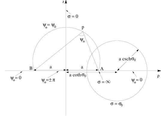
FIG. 1.: Toroidal coordinates $\sigma$, $\psi_{*}$ is defined on the extension of a $\varphi$=constant half-plane in Euclidean space. $A$ and $B$ are the points at which the equatorial circle $\rho=a$ intersects this plane. For any point $P(\sigma,\psi_{*},\varphi)$, $\sigma=\ln(AP/PB)$, and $\psi_{*}=\pm$(angle $APB$), with the sign equal to the sign of $z$.

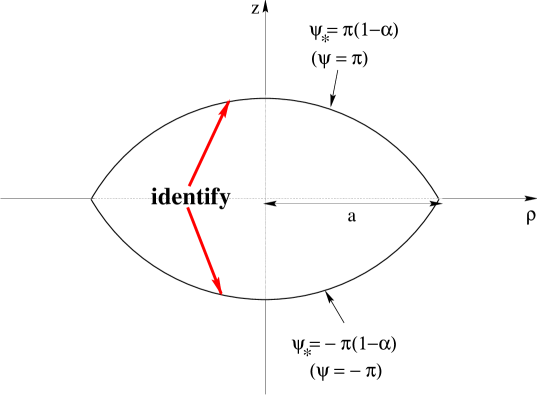
FIG. 2.: The conformally flat geometry of the circular string loop, located at $\rho=a$ in this Euclidean map, is constructed by conformally squeezing the two spherical caps $\psi_{*}=\pm\pi(1-\alpha)$ to become in effect, equatorial disks spanning the loop, and topologically identifying them.

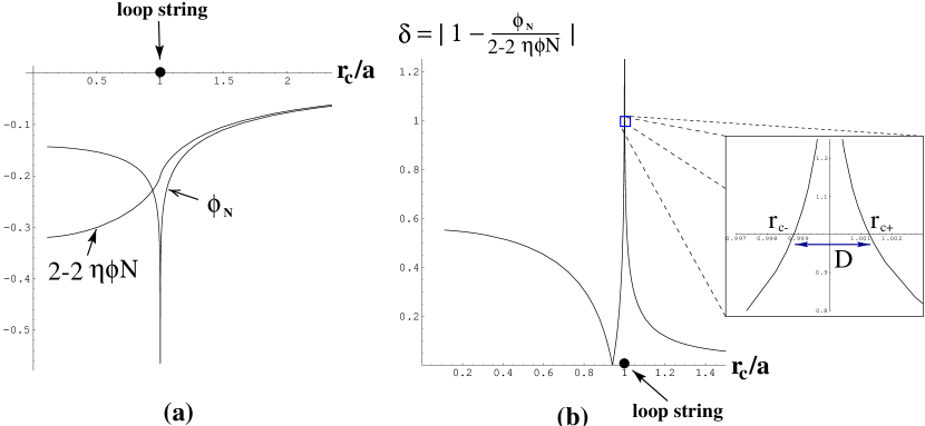
FIG. 3.: (a) $2(1-\eta\phi N)$ and $\phi_{N}$ in the equatorial plane with $\alpha=0.1$ are drawn at the same circumference radius $r_{c}$ of the Killing orbit of $\varphi^{a}$ normalized by the loop radius $a$. (b) From $2(1-\eta\phi N)$ and $\phi_{N}$, we obtain the profile of $\delta=|1-\phi_{N}/(2-2\eta\phi N)|$.

FIG. 4.: The criterion $D$ of a cosmic string thickness for each deficit angle $\alpha$ is shown. $a$ is the loop radius. We may say that the linear perturbation theory around flat Euclid space fails to describe the gravity of a string when the string thickness is smaller than $D$.

REFERENCES

- [1] A. Vilenkin and E.P.S. Shellard, “Cosmic Strings and Other Topological Defects”, (Cambridge University Press, Cambridge, England, 1994). E.W. Kolb and M.S. Turner, The Early Universe, (Addison-Wesly Publishing Company, 1993).
- [2] A. Vilenkin, and A.E. Everett Phys. Rev. Lett. 48 1867, (1982). T. Vachaspati, A.E. Everett and A. Vilenkin, Phys. Rev. D30 2046, (1984). T. Vachaspati, Nucl. Phys. B277, 593, (1986). M. Sakellariadou, Phys. Rev. D42, 345, (1990). R.R.. Caldwell and B. Allen, ibid., 45, 3447, (1992). P. Casper and B. Allen, ibid., 52, 4337, (1995). B. Allen and A.C. Ottewill, Phys. Rev. D63, 063507, (2001).
- [3] R.A. Battye and E.P.S. Shellard, Class. Quantum Grav. 13 A239, (1996). R.R. Caldwell, R.A. Battye and E.P.S. Shellard, Phys. Rev. D54, 7146, (1996).
- [4] K. Nakamura A. Ishibashi and H. Ishihara, Phys. Rev. D62, 101502R, (2000). K. Nakamura and H. Ishihara, ibid., 63, 127501, (2001).
- [5] W. Israel, Phys. Rev. D15, 935, (1977). M. Hindmarsh, Phys. Lett. B251, 28, (1990). R. Gregory, D. Haws and D. Garfinkle, Phys. Rev. D42, 343, (1990). B. Carter, Phys. Rev. Lett. 74, 3098, (1995). R.A. Battye and B. Carter, Phys. Lett. B357, 29, (1995). B. Boisseau, C. Charmousis and B. Linet, ibid., 55, 616, (1997). C.J.S. Clarke, J.A. Vickers and J.P. Wilson, Class. Quantum Grav., 13, 2485, (1996). J.A. Vickers and J.P. Wilson, ibid., 16, 579, (1999). D. Garfinkle, ibid., 16, 4101, (1999). R.A. Battye and B. Carter, ibid., 17, 3325, (2000).
- [6] R. Geroch and J. Traschen, Phys. Rev. D36, 1017, (1987).
- [7] W. Kinnersley and M. Walker, Phys. Rev. D2, 1359, (1970). D. Kramer, H. Stephani, M.A.H. MacCallum and E. Herlt, Exact Solutions of Einstein’s Field Equations (Cambridge: Cambridge University Press, 1980).
- [8] D. Garfinkle, Phys. Rev. D32, 1323, (1985). R. Gregory, Phys. Rev. Lett. 59, 740,(1987). T. Futamase and D. Garfinkle, Phys. Rev. D37, 2086, (1988).
- [9] W.G. Unruh, G. Hayward, W. Israel and D. McManus, Phys. Rev. Lett. 62, 2897, (1989).
- [10] V.P. Frolov, W. Israel and W.G. Unruh, Phys. Rev., D39, 1084, (1989).
- [11] B. Boisseau, C. Charmousis, and B. Linet, Phys. Rev. D55, 616, (1997).
- [12] R.M. Wald General Relativity (Univ. of Chicago Press, Chicago, 1984).
- [13] W. Israel, Nuovo Cimento B44 (1966), 1.
- [14] T. Damour and A. Vilenkin, Phys. Rev. Lett. 85, 3761, (2000).