A cosmological model in Weyl-Cartan spacetime

Abstract

We present a cosmological model for early stages of the universe on the basis of a Weyl-Cartan spacetime. In this model, torsion $T^{\alpha}$ and nonmetricity $Q_{\alpha\beta}$ are proportional to the vacuum polarization. Extending earlier work of one of us (RT), we discuss the behavior of the cosmic scale factor and the Weyl 1-form in detail. We show how our model fits into the more general framework of metric-affine gravity (MAG).

1 Introduction

We present a scale invariant model for early stages of the universe. Spacetime is described by a Weyl-Cartan geometry. The torsion and nonmetricity become proportional to the Weyl 1-form $Q$. Our starting point is the work of Tresguerres [6], which will be discussed here in more detail. The plan of the paper is as follows. In section 2 we derive the field equations and thereby recover the results found in [6]. In sections 3–5, we discuss the behavior of the cosmic scale factor $S(t)$ and that of the Weyl 1-form $Q$, which governs the non-Riemannian features of the model. We provide a list of the explicit form of the surviving curvature pieces for each branch of the solution. Additionally, we investigate the question of whether the solution exhibits singularities. In A we make contact with the formalism used in metric-affine gauge theory of gravity as proposed by Hehl et alin [3]. Finally, in B, we show how the geometric quantities occurring in MAG have to be constrained in case of a Weyl-Cartan spacetime.

2 Cosmology in a Weyl-Cartan spacetime

Following the model proposed in [6], we confine ourselves to a Weyl-Cartan spacetime $Y_{4}$. For a brief introduction into the Weyl-Cartan subcase of MAG see B. We start start with the following Lagrangian ($R_{\alpha\beta}=W_{\alpha\beta}+Z_{\alpha\beta}=$ antisymmetric $+$ symmetric part of the curvature):

$$V = \frac{\chi}{2\kappa}R_{\alpha}{}^{\beta}\wedge\eta_{\beta}\,^{\alpha}+\sum\limits_{I=1}^{6}a_{I}\,\,^{(I)}W_{\alpha}{}^{\beta}\wedge\,^{\star}R_{\beta}\,^{\alpha}+b\,Z_{\alpha\beta}\wedge\,^{\star}R^{\beta\alpha}$$ (2)

$$= \texttt{\rm Einstein-Hilbert}+\texttt{\rm quadratic rotational curvature}$$

$$+\texttt{\rm quadratic strain curvature,}$$

with $\chi,$ $a_{I=1..6},$ $b$ arbitrary constants and $\kappa$ being the weak coupling constant. Here we make use of the irreducible decomposition of the curvature as presented in [4]. The matter Lagrangian $L_{{\rm mat}}\,$is not explicitly given, but will later on be introduced in a phenomenological way. From (2) we calculate the gauge field excitations (cf. A, eqs. (97)-(99)):

$$H_{\alpha} = 0,\quad M^{\alpha\beta}=0,$$ (3)

$$H^{\alpha}{}_{\beta} = -\frac{\chi}{2\kappa}\eta_{\beta}{}^{\alpha}-2\sum_{I=1}^{6}a_{I}\,\,^{\star(I)}W_{\beta}{}^{\alpha}-\frac{b}{2}\delta_{\beta}^{\alpha}\,{}^{\star}R^{\gamma}{}_{\gamma}.$$ (4)

The canonical energy-momentum is given by

$$E_{\alpha} = e_{\alpha}\rfloor V+\left(e_{\alpha}\rfloor R_{\beta}{}^{\gamma}\right)\wedge H^{\beta}{}_{\gamma}+\left(e_{\alpha}\rfloor T^{\beta}\right)\wedge H_{\beta}+\frac{1}{2}\left(e_{\alpha}\rfloor Q_{\beta\gamma}\right)\wedge M^{\beta\gamma}$$ (5)

$$= e_{\alpha}\rfloor V+\left(e_{\alpha}\rfloor R_{\beta}{}^{\gamma}\right)\wedge H^{\beta}{}_{\gamma}.$$ (6)

Because of (3), the hypermomentum vanishes

$$E^{\alpha}{}_{\beta}=-\vartheta^{\alpha}\wedge H_{\beta}-g_{\beta\gamma}M^{\alpha\gamma}=0.$$ (7)

The field equations in a Weyl-Cartan spacetime (cf. B) now turn into

$$-E_{\alpha} = \Sigma_{\alpha,}$$ (8)

$$dH^{\alpha}{}_{\alpha} = \Delta,$$ (9)

$$g_{\gamma[\alpha}DH^{\gamma}\,_{\beta]} = \tau_{\alpha\beta}.$$ (10)

Following [6], we consider a non-massive medium without spin, i.e. the spin current is assumed to vanish $\tau_{\alpha\beta}\stackrel{{\scriptstyle A}}{{=}}0$ (this can also be interpreted as a spin current which averages out on macroscopic scales). Thus, our medium is equipped only with a dilation current $\Delta$ and eq. (10) turns into

$$g_{\gamma[\alpha}DH^{\gamma}\,_{\beta]}=0.$$ (11)

In addition to (8), (9) and (11), one has to consider the Noether identities (cf. B). They play the role of consistency conditions, since the matter Lagrangian is not explicitly given. For a vanishing spin current the second identity (cf. eqs. (112), (113)) turns into

$$\frac{1}{4}g_{\alpha\beta}\,d\Delta+\vartheta_{(\alpha}\wedge\Sigma_{\beta)} = \sigma_{\alpha\beta},$$ (12)

$$\vartheta_{[\alpha}\wedge\Sigma_{\beta]} = 0.$$ (13)

Taking eq. (9) into account, (12) turns into

$$\vartheta_{(\alpha}\wedge\Sigma_{\beta)}=\sigma_{\alpha\beta}.$$ (14)

The first identity (114) becomes

$$D\Sigma_{\alpha}\stackrel{{\scriptstyle\tau_{\alpha\beta}=0\,,\,(\ref{second_noether_treguerres_final_1})}}{{=}}\left(e_{\alpha}\rfloor T^{\beta}\right)\wedge\Sigma_{\beta}-\frac{1}{2}\left(e_{\alpha}\rfloor Q\right)\,\vartheta^{\beta}\wedge\Sigma_{\beta}+\frac{1}{4}\left(e_{\alpha}\rfloor R\right)\wedge\Delta.$$ (15)

Thus, we have to solve (8), (9), (11), (13), (14), and (15) in order to obtain a solution of the MAG field equations (93)-(96).

Next we turn to the description of the matter sources. For a vanishing spin current in a Weyl-Cartan spacetime (cf. eq. (109)) the hypermomentum $\Delta_{\alpha\beta}$ becomes proportional to its trace part, i.e. reduces to the dilation contribution

$$\Delta_{\alpha\beta}=\frac{1}{4}g_{\alpha\beta}\Delta.$$ (16)

The trace part (9) of the second field equation yields

$$d\Delta=0\quad\Rightarrow\quad\exists\,\,\texttt{\rm 2-form }P:\quad dP=\Delta.$$ (17)

Consequently, the dilation current is conserved and there exists a 2-form $P$ being a potential for $\Delta$. We call this form polarization 2-form, the most obvious choice would be

$$P\stackrel{{\scriptstyle A}}{{=}}H^{\gamma}{}_{\gamma}=-2b\,^{\star}R=-2b\,^{\star}R^{\gamma}{}_{\gamma}.$$ (18)

Of course, this ansatz automatically satisfies (9). Guided by (18) we assume $P$ to be of the form

$$P=f(t,r)\,\vartheta^{\alpha}\wedge\vartheta^{\beta}.$$ (19)

So far, $\alpha$ and $\beta$ represent unspecified coframe indices (we fix them when introducing the coframe), and $f(t,r)$ denotes an arbitrary function of the time and radial coordinate. After fixing the general form of the hypermomentum current, we have to specify the energy-momentum 3-form which appears in (8), (13), (14), and (15). Equation (13) forces $\Sigma_{\alpha}$ to be symmetric. Consequently, we choose

$$\Sigma_{\alpha}\stackrel{{\scriptstyle A}}{{=}}\Sigma_{\alpha\beta}\,\eta^{\beta},$$ (20)

where $\Sigma_{\alpha\beta}=\,$diag$(\mu,p_{r},p_{t},p_{t})$ and $\mu=\mu(t),$ $p_{r}=p_{r}(t),$ $p_{t}=p_{t}(t)$ denote the energy density, and the radial and tangential stresses. Taking (14) into account, one obtains the relation

$$\sigma^{\gamma}{}_{\gamma}\stackrel{{\scriptstyle(\ref{second_noether_treguerres_final_1})}}{{=}}\,\vartheta^{\gamma}\wedge\Sigma_{\gamma} = \vartheta^{\gamma}\wedge\left(\Sigma_{\gamma\beta}\eta^{\beta}\right)=\Sigma_{\gamma\beta}\,\left(\vartheta^{\gamma}\wedge\eta^{\beta}\right)$$ (21)

$$= \Sigma_{\gamma\beta}\,\left(\vartheta^{\gamma}\wedge\,^{\star}\vartheta^{\beta}\right)=\Sigma_{\gamma\beta}\left(\left(-1\right)^{1-1}g^{\gamma\beta}\,\,{}^{\star}1\right)$$

$$= \Sigma_{\gamma\beta}\,g^{\gamma\beta}\eta=\Sigma^{\gamma}{}_{\gamma}\eta=(\mu-p_{r}-2p_{t})\eta.$$

Now we are going to fix the underlying metrical structure. Following the standard cosmological model (cf. [1]), we take the Robertson-Walker line element as starting point.

$$\vartheta^{\hat{0}}=dt,\quad\vartheta^{\hat{1}}=\frac{S(t)}{\sqrt{1-kr^{2}}}dr,\quad\vartheta^{\hat{2}}=S(t)\,r\,d\theta,\quad\vartheta^{\hat{3}}=S(t)\,r\,\sin\theta d\phi,$$ (22)

with the line element

$$ds^{2}\stackrel{{\scriptstyle A}}{{=}}\vartheta^{\hat{0}}\otimes\vartheta^{\hat{0}}-\vartheta^{\hat{1}}\otimes\vartheta^{\hat{1}}-\vartheta^{\hat{2}}\otimes\vartheta^{\hat{2}}-\vartheta^{\hat{3}}\otimes\vartheta^{\hat{3}}.$$ (23)

As usual, $S(t)$ denotes the cosmic scale factor and $k=-1,0,1$ determines whether the spatial sections are of constant negative, vanishing or positive curvature. Thus, we look for spherically symmetric solutions. This choice fixes the indices in (19) to be $\alpha=\hat{2}$ and $\beta=\hat{3}$. Additionally, we impose another constraint on the so called polarization function $f(t,r)$ in (19) by allowing only for functions which depend on the time coordinate, i.e.$\,f(r,t)\stackrel{{\scriptstyle A}}{{\rightarrow}}\frac{\xi(t)}{S^{2}(t)}$. Consequently, our ansatz made in (19) turns into

$$P=\frac{\xi(t)}{S^{2}(t)}\vartheta^{\hat{2}}\wedge\vartheta^{\hat{3}}\texttt{\rm,}$$ (24)

where $\xi(t)$ represents the new arbitrary polarization function. Equation (24) yields the form of the dilation current $\Delta$ to be

$$\Delta = dP=\frac{2\xi\sqrt{1-kr^{2}}}{S^{3}r}\vartheta^{\hat{1}}\wedge\vartheta^{\hat{2}}\wedge\vartheta^{\hat{3}}+\frac{\dot{\xi}}{S^{2}}\vartheta^{\hat{0}}\wedge\vartheta^{\hat{2}}\wedge\vartheta^{\hat{3}}$$ (25)

$$= \frac{2\xi\sqrt{1-kr^{2}}}{S^{3}r}\eta^{\hat{0}}+\frac{\dot{\xi}}{S^{2}}\eta^{\hat{1}}.$$ (26)

The next thing to come up is a proper ansatz for the torsion 2-form $T^{\alpha}$. We choose the torsion to be proportional to its vector piece$\,T^{\alpha}\sim\,^{(2)}T^{\alpha}$ which is proportional to the Weyl 1-form

$$T^{\alpha}\stackrel{{\scriptstyle A}}{{=}}\frac{1}{2}Q\wedge\vartheta^{\alpha}.$$ (27)

We are now going to calculate the Weyl 1-form from the trace part of the second field equation (9). Using (25), eq. (9) turns into

$$dH^{\gamma}{}_{\gamma}=\Delta=dP.$$ (28)

From (4) we subsequently deduce

$$dH^{\gamma}{}_{\gamma}=-2b\,d^{\star}R\stackrel{{\scriptstyle{\rm(Weyl-Cartan)}}}{{=}}-4b\,d^{\star}dQ.$$ (29)

Putting the last two equations together we obtain

$$-4bd\,^{\star}dQ = dP,$$ (30)

$$\Rightarrow\,^{\star}dQ = -\frac{P}{4b}\Rightarrow dQ=\frac{\xi}{4bS^{2}}\vartheta^{\hat{0}}\wedge\vartheta^{\hat{1}},$$ (31)

$$\Rightarrow\quad\,Q = -\frac{\xi}{4bS}\left(\int dr\frac{1}{\sqrt{1-kr^{2}}}\right)\vartheta^{\hat{0}}+\texttt{\rm exact contribution.}$$ (32)

Neglecting the trivial exact contribution, we obtain the following explicit expressions for $Q,$ which depend on the sign of the spatial curvature:

$$Q =-\frac{\xi(t)}{4bS(t)}\,\texttt{\rm arcsinh}\left(r\right)\,\vartheta^{\hat{0}}\quad \texttt{\rm for }k=-1,$$ (33)

$$Q =-\frac{\xi(t)}{4bS(t)}\,r\,\vartheta^{\hat{0}}\quad \texttt{\rm for }k=0,$$ (34)

$$Q =-\frac{\xi(t)}{4bS(t)}\,\texttt{\rm arcsin}\left(r\right)\,\vartheta^{\hat{0}}\quad \texttt{\rm for }k=1.$$ (35)

We calculate the field equations resulting from the second Noether identity in (14). We make use of computer algebra and obtain two independent equations, namely

$$\frac{d}{dt}\left(\mu S^{4}+\frac{\xi^{2}}{16b}\right) = \frac{1}{4}\left(\mu-p_{r}-2p_{t}\right)\,\frac{dS^{4}}{dt},$$ (36)

$$p_{r}-p_{t} = \frac{\xi^{2}}{8bS^{4}}.$$ (37)

We make use of eq. (37) and rewrite the energy-momentum trace

$$\Sigma^{\gamma}{}_{\gamma}=\mu-p_{r}-2p_{t}=\mu-3p_{t}-\frac{\xi^{2}}{8bS^{4}}.$$ (38)

Let us now inspect the remaining field equations, i.e. the antisymmetric part of the second equation (11), called the spin equation, and the first field equation (8). By use of computer algebra, we investigate eq. (11) and obtain one independent equation, namely

$$\left(a_{4}+a_{6}\right)\bigg{(}\stackrel{{\scriptstyle...}}{{S}}S^{2}+\ddot{S}\dot{S}S-2\dot{S}^{3}-2k\dot{S}\bigg{)}=0.$$ (39)

Thus, for $a_{6}\neq-a_{4}$ and after some algebra, this equation turns into

$$\frac{d}{dt}\left(\frac{\ddot{S}}{S}+\left(\frac{\dot{S}}{S}\right)^{2}+\frac{k}{S^{2}}\right)=0.$$ (40)

Hereby we recovered one of the field equations given in [6] eq. (3.7). Now we draw our attention to the first field equation. Eq. (8) yields three independent equations, namely

$$\chi\left(\left(\frac{\dot{S}}{S}\right)^{2}+\frac{k}{S^{2}}\right)-\kappa\left(a_{4}+a_{6}\right)\left(\left(\frac{\ddot{S}}{S}\right)^{2}-\left(\left(\frac{\dot{S}}{S}\right)^{2}+\frac{k}{S^{2}}\right)^{2}\right)$$

$$=\frac{\kappa}{3}\left(\mu+\frac{\xi^{2}}{16bS^{4}}\right),$$ (41)

$$\chi\left(2\frac{\ddot{S}}{S}+\left(\frac{\dot{S}}{S}\right)^{2}+\frac{k}{S^{2}}\right)+\kappa\left(a_{4}+a_{6}\right)\left(\left(\frac{\ddot{S}}{S}\right)^{2}-\left(\left(\frac{\dot{S}}{S}\right)^{2}+\frac{k}{S^{2}}\right)^{2}\right)$$

$$=-\kappa\left(p_{r}-\frac{\xi^{2}}{16bS^{4}}\right),$$ (42)

$$\chi\left(2\frac{\ddot{S}}{S}+\left(\frac{\dot{S}}{S}\right)^{2}+\frac{k}{S^{2}}\right)+\kappa\left(a_{4}+a_{6}\right)\left(\left(\frac{\ddot{S}}{S}\right)^{2}-\left(\left(\frac{\dot{S}}{S}\right)^{2}+\frac{k}{S^{2}}\right)^{2}\right)$$

$$=-\kappa\left(p_{t}+\frac{\xi^{2}}{16bS^{4}}\right).$$ (43)

Comparison with the results in [6] reveals the equivalence of (41), (43) and eqs. (3.8),(3.9) of [6]. We make use of some algebra in order to write (41)-(43) in a more convenient form. By adding (41) and (43) we obtain

$$\chi\left(2\frac{\ddot{S}}{S}+2\left(\frac{\dot{S}}{S}\right)^{2}+2\frac{k}{S^{2}}\right) = \frac{\kappa}{3}\left(\mu+\frac{\xi^{2}}{16bS^{4}}\right)-\kappa\left(p_{t}+\frac{\xi^{2}}{16bS^{4}}\right)$$

$$\Leftrightarrow 2\chi\left(\frac{\ddot{S}}{S}+\left(\frac{\dot{S}}{S}\right)^{2}+\frac{k}{S^{2}}\right) = \frac{\kappa}{3}\left(\mu-3p_{t}-\frac{\xi^{2}}{8bS^{4}}\right).$$ (44)

Subtracting (43) from (41) yields

$$2\chi\frac{\ddot{S}}{S}+2\kappa\left(a_{4}+a_{6}\right)\left(\left(\frac{\ddot{S}}{S}\right)^{2}-\left(\left(\frac{\dot{S}}{S}\right)^{2}+\frac{k}{S^{2}}\right)^{2}\right)$$

$$=-\frac{\kappa}{3}\left(\mu+3p_{t}+\frac{\xi^{2}}{4bS^{4}}\right).$$ (45)

Closer examination of (44) and (40) leads to

$$0 \stackrel{{\scriptstyle(\ref{tresguerre_eq_4_13})}}{{=}} \frac{d}{dt}\left(\frac{\ddot{S}}{S}+\left(\frac{\dot{S}}{S}\right)^{2}+\frac{k}{S^{2}}\right)\stackrel{{\scriptstyle(\ref{addierte_Feldgleichungen_1_tresguerres})}}{{=}}\frac{\kappa}{3}\frac{d}{dt}\left(\mu-3p_{t}-\frac{\xi^{2}}{8bS^{4}}\right)$$ (46)

$$\stackrel{{\scriptstyle(\ref{energy_momentum_trace_tresguerres})}}{{=}} \frac{\kappa}{3}\frac{d\Sigma^{\gamma}{}_{\gamma}}{dt}\quad\Rightarrow\quad\Sigma^{\gamma}{}_{\gamma}=\mu-p_{r}-2p_{t}=\texttt{\rm constant}=:\Xi.$$ (47)

Thus, the trace of the energy-momentum turns out to be a constant. We will now investigate the consequences of a vanishing energy-momentum trace $\Xi$. In order to extract some information from the assumption $\Xi\stackrel{{\scriptstyle A}}{{=}}0,$ we rewrite eq. (36) by making use of the following definitions:

$$\tilde{\mu}:=\mu+\frac{\xi^{2}}{16bS^{4}},\quad\quad\tilde{p}:=\frac{1}{3}\tilde{\mu}.$$ (48)

We call $\tilde{\mu}$ and $\tilde{p}$ effective energy and pressure, respectively. After some algebra, we find that (36) is equivalent to

$$d\left(\tilde{\mu}S^{3}\right)=-\left(\tilde{p}-\frac{\Xi}{3}\right)dS^{3}.$$ (49)

This equation has the character of a thermodynamical relation and shows that in case of $\Xi=0$ the constant contribution to the effective pressure on the r.h.s. vanishes. Consequently, the following relations hold in case of $\Xi=0$:

$$\mu \stackrel{{\scriptstyle(\ref{trace_ist_costant})}}{{=}} p_{r}+2p_{t}$$ (50)

$$\stackrel{{\scriptstyle(\ref{sec_noether_explicit2_final})}}{{\Rightarrow}} p_{r}=\frac{1}{3}\left(\mu+\frac{\xi^{2}}{4bS^{4}}\right)\quad\Rightarrow\quad p_{t}=\frac{1}{3}\left(\mu-\frac{\xi^{2}}{8bS^{4}}\right).$$ (51)

From the second Noether identity in (36) we gain $\mu=\mu(t)$ as a function of the polarization function $\xi(t)$ and the scale factor as follows:

$$\frac{d}{dt}\left(\mu S^{4}+\frac{\xi^{2}}{16b}\right)=0\quad\Rightarrow\quad\mu=-\frac{\xi^{2}}{16bS^{4}}+\frac{\mu_{0}}{S^{4}},$$ (52)

where $\mu_{0}$ represents an integration constant. The stresses in (51) take the form

$$p_{r}=\frac{\mu_{0}}{3S^{4}}+\frac{\xi^{2}}{16bS^{4}},\quad\quad p_{t}=\frac{\mu_{0}}{3S^{4}}-\frac{\xi^{2}}{16bS^{4}},$$ (53)

i.e. are equal if the polarization function $\xi(t)$ vanishes. Once again, we consider the field equations. From eq. (40) follows

$$\frac{\ddot{S}}{S}+\left(\frac{\dot{S}}{S}\right)^{2}+\frac{k}{S^{2}}=\texttt{\rm const}:=\frac{2}{3}\Lambda.$$ (54)

Note that we are free to choose the emerging constant. Comparison with the classical Friedman equations reveals that this constant plays a role similar to that of the cosmological constant. Thus, we call $\Lambda$ induced cosmological constant. For vanishing trace the field equation (44) becomes

$$2\chi\left(\frac{\ddot{S}}{S}+\left(\frac{\dot{S}}{S}\right)^{2}+\frac{k}{S^{2}}\right)=0,$$ (55)

by insertion of (54) we arrive at

$$\chi\Lambda=0.$$ (56)

We make use of (52), (53), and (54) and rewrite the remaining field equation (45) as

$$\chi\frac{\ddot{S}}{S}+\frac{4\kappa\Lambda}{3}\left(a_{4}+a_{6}\right)\left(\frac{\ddot{S}}{S}-\frac{\Lambda}{3}\right)=-\frac{\kappa\mu_{0}}{3S^{4}},$$ (57)

in accordance with the result obtained in [6] eq. (3.14).

Before we discuss possible solutions of the model under consideration, we will shortly collect all assumptions made up to here in table 1.

Table 1: Assumptions made up to this point.

• Ansatz/assumption	Resulting quantity/equations	Equation number
  $\tau_{\alpha\beta}=0$	$g_{\gamma[\alpha}DH^{\gamma}{}_{\beta]}=0$	(11)
  $P=\frac{\xi}{S^{2}}\vartheta^{\hat{2}}\wedge\vartheta^{\hat{3}}$	$\Delta,Q,$ $dH^{\gamma}{}_{\gamma}\equiv 0$	(16),(30),(9)
  $T^{\alpha}=\frac{1}{2}Q\wedge\vartheta^{\alpha}$	Affects form of the connection	(108)
  $\left(a_{4}+a_{6}\right)\neq 0$	Affects form of the spin equation	(40)
  $\Xi=0=\Sigma^{\gamma}{}_{\gamma}$	$\mu$, $\,p_{r}$, $\,p_{t}$, form of the field eqs, $\Lambda$	(52),(53),(54)
  $\Lambda$	Affects form of the field eqs.	(55)-(57)

The final form of the field equations is given by (54), (56), (57), i.e.

$$\frac{\ddot{S}}{S}+\left(\frac{\dot{S}}{S}\right)^{2}+\frac{k}{S^{2}} = \frac{2}{3}\Lambda,$$ (58)

$$\chi\Lambda = 0,$$ (59)

$$\chi\frac{\ddot{S}}{S}+\frac{4\kappa\Lambda}{3}\left(a_{4}+a_{6}\right)\left(\frac{\ddot{S}}{S}-\frac{\Lambda}{3}\right) = -\frac{\kappa\mu_{0}}{3S^{4}}.$$ (60)

3 Vacuum solution

We are now going to solve the system (58)-(60). We start by putting $\chi=0$, i.e. the Einstein-Hilbert term in the Lagrangian (2) is assumed to vanish. Since the Einstein-Hilbert term is supposed to describe physics at low energies, we expect the upcoming solution to be valid only in very early stages of the universe, i.e. at high energies. We note that our ansatz fulfills (59) and try to solve (58) for nonvanishing $\Lambda$. We can verify that

$$S(t)=A\,e^{\sqrt{\frac{\Lambda}{3}}t}+\frac{3k}{4A\Lambda}\,e^{-\sqrt{\frac{\Lambda}{3}}t}\quad\quad\texttt{\rm, with }A=\texttt{\rm const,}$$ (61)

satisfies eq. (58). Insertion of (61) into (60) with $\chi=0$, yields

$$\frac{4\kappa\Lambda}{3}\left(a_{4}+a_{6}\right)\left(\frac{\ddot{S}}{S}-\frac{\Lambda}{3}\right)=-\frac{\kappa\mu_{0}}{3S^{4}}\quad\rightarrow\quad\kappa\mu_{0}\Lambda^{4}A^{4}e^{4\sqrt{\frac{\Lambda}{3}}t}=0.$$ (62)

Thus, we have to choose $\mu_{0}=0$ in order to fulfill (60). From eq. (52) we derive the final expressions of the energy and stresses

$${}^{{\rm vac}}\mu=-\frac{\xi^{2}}{16bS^{4}}\quad\Rightarrow\quad\,^{{\rm vac}}\tilde{\mu}=0\quad\stackrel{{\scriptstyle(\ref{stresses_for_xi_zero_2})}}{{\Rightarrow}}\quad\,^{{\rm vac}}p_{r}=-\,^{{\rm vac}}p_{t}=-\,^{{\rm vac}}\mu.$$ (63)

In view of (63), it becomes clear why this branch of our model is the called vacuum solution. Note that in contrast to the standard result, the vacuum energy ${}^{{\rm vac}}\mu$ is not a constant and proportional to the polarization function $\xi(t)$. Finally, the Weyl 1-form reads

$$Q =-\frac{\xi(t)}{4bA\,e^{\sqrt{\frac{\Lambda}{3}}t}-\frac{3b}{\Lambda A}\,e^{-\sqrt{\frac{\Lambda}{3}}t}}\,\,\texttt{\rm arcsinh}(r)\,\vartheta^{\hat{0}}\quad\quad \texttt{\rm for }k=-1\texttt{\rm,}$$ (64)

$$Q =-\frac{\xi(t)r}{4bA\,e^{\sqrt{\frac{\Lambda}{3}}t}}\,\vartheta^{\hat{0}}\quad\quad \texttt{\rm for }k=0\texttt{\rm,}$$ (65)

$$Q =-\frac{\xi(t)}{4bA\,e^{\sqrt{\frac{\Lambda}{3}}t}+\frac{3b}{\Lambda A}\,e^{-\sqrt{\frac{\Lambda}{3}}t}}\,\,\texttt{\rm arcsin}(r)\vartheta^{\hat{0}}\quad\quad \texttt{\rm for }k=1\texttt{\rm.}$$ (66)

We observe that the only surviving pieces of the curvature are ${}^{(6)}W_{\alpha\beta}\,$ and ${}^{(4)}Z_{\alpha\beta}$. Their nonvanishing components read as follows:

$${}^{(6)}W^{\alpha\beta} = \frac{\Lambda}{3}\vartheta^{\alpha}\wedge\vartheta^{\beta},$$ (67)

$${}^{(4)}Z_{\hat{0}\hat{0}} = \frac{2A^{2}\Lambda^{2}e^{2\sqrt{\frac{\Lambda}{3}}t}\xi(t)}{b\left(16A^{4}\Lambda^{2}e^{4\sqrt{\frac{\Lambda}{3}}t}+24kA^{2}\Lambda e^{2\sqrt{\frac{\Lambda}{3}}t}+9\right)}\vartheta^{\hat{0}}\wedge\vartheta^{\hat{1}}$$ (68)

$$= \,-^{(4)}Z_{\hat{1}\hat{1}}=\,-^{(4)}Z_{\hat{2}\hat{2}}=-\,^{(4)}Z_{\hat{3}\hat{3}}\texttt{\rm.}$$

Note that the results collected in (67) and (68) are valid for $k=-1,0,1$. The torsion and nonmetricity read

$${}^{(2)}T^{\hat{0}} =0,\quad\quad\quad^{(2)}T^{a} =\frac{1}{2}Q\wedge\vartheta^{a},$$ (69)

$${}^{(4)}Q_{\hat{0}\hat{0}} =Q=-\,^{(4)}Q_{\hat{1}\hat{1}} =\,-\,^{(4)}Q_{\hat{2}\hat{2}}=\,-\,^{(4)}Q_{\hat{3}\hat{3}}.\,\,$$ (70)

We continue with the calculation of the curvature invariant $\,{}^{\star}\left(R_{\alpha\beta}\wedge\,^{\star}R^{\alpha\beta}\right)$ in order to answer the question of whether our solution possesses essential singularities or not. In table 2, we display parameter values and times at which an essential singularity emerges. In the case of $t_{{\rm div}}$ these are the epochs of the universe at which the invariant diverges. Note that not listed variables and parameters are allowed to take arbitrary values.

Table 2: Parameter values and times with essential singularities (vacuum solution).

• $k=-1$	$\{t_{{\rm div}}=\frac{\sqrt{3}}{2}\frac{\ln\left(\frac{3}{A^{2}\Lambda}\right)}{\sqrt{\Lambda}}\}$ or $\{b=0\}$
  $k=0$	$\{A=0\}$ or$\,\,\,\{b=0\}$
  $k=1$	$\{t_{{\rm div}}=\frac{\sqrt{3}}{2}\frac{\ln\left(-\frac{3}{A^{2}\Lambda}\right)}{\sqrt{\Lambda}}\}\,$or $\{b=0\}$

In figure 1 we display the function $t=t_{{\rm div}}(A,\Lambda)$ in the case of $k=-1$.

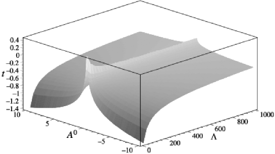
Figure 1: Plot of the times $t=t_{\rm div}$ at which the vacuum solution becomes singular in case of $k=-1$.

As can be read of from there, our solution exhibits no singularity as long as $A$ vanishes. In the light of (61) this choice is only allowed if $k=0$. Consequently, our solution always exhibits a singularity after a finite time as long as $\Lambda\in\,]0,\infty[$ (negative values of $\Lambda$ can be ruled out since they lead to a complex valued scale factor $S(t)$). Reinsertion of the expression for $t_{{\rm div}}(A,\Lambda)$ into the solution for the cosmic scale factor, as stated in (61), reveals that we are dealing with a point singularity at the origin of the universe, i.e. $S(t_{{\rm div}})=0$. Thus, this type of singularity is similar to those known from the Riemannian case. In case of a vanishing $k$ there is no singularity since $b=0$ leads to a constraint in our Lagrangian and $A=0$ corresponds to the unphysical solution $S(t)\equiv 0$.

Figure 2: Scale factor $S$ and the function $Q$ (which governs the Weyl 1-form) in case of the vacuum ($\Lambda\neq 0$, $\chi=0$) solution.

4 Intermediate vacuum solution

At this point we will briefly mention a solution in case of $\chi=\Lambda=0\neq k$. Under this assumption eq. (59) is fulfilled identically. Equation (58) and (60) turn into

$$\frac{\ddot{S}}{S}+\left(\frac{\dot{S}}{S}\right)^{2}+\frac{k}{S^{2}} = 0,$$ (71)

$$-\frac{\kappa\mu_{0}}{3S^{4}} = 0.$$ (72)

It is straightforward to check that

$$S(t)=\sqrt{F-k\,t^{2}},\texttt{\rm\quad\quad with\quad}F=\texttt{\rm const,}$$ (73)

is a solution of (71). From (72) we recover the same relation between the energy and stresses as in (63). Thus, this solution belongs to the vacuum regime, too. The final form of the Weyl 1-form reads

$$Q =-\frac{\xi(t)}{4b\sqrt{F+t^{2}}}\,\,\texttt{\rm arcsinh}(r)\,\vartheta^{\hat{0}}\quad\quad \texttt{\rm for }k=-1,$$ (74)

$$Q =-\frac{\xi(t)}{4b\sqrt{F-t^{2}}}\,\,\texttt{\rm arcsin}(r)\,\vartheta^{\hat{0}}\quad\quad \texttt{\rm for }k=1.$$ (75)

The surviving curvature components are given by

$${}^{(4)}Z_{\hat{0}\hat{0}} = \frac{\xi(t)}{8b\left(F-kt^{2}\right)}\vartheta^{\hat{0}}\wedge\vartheta^{\hat{1}}=-\,^{(4)}Z_{\hat{1}\hat{1}}=-\,^{(4)}Z_{\hat{2}\hat{2}}=-\,^{(4)}Z_{\hat{3}\hat{3}}\texttt{\rm,}$$ (76)

$${}^{(4)}W^{\alpha\beta} = \frac{kF}{\left(F-kt^{2}\right)^{2}}\vartheta^{\alpha}\wedge\vartheta^{\beta}\texttt{\rm,}$$ (77)

The parameter values and epochs at which the curvature invariant diverges are collected in table 3.

Table 3: Parameter values and times with essential singularities (intermediate solution).

• $k=-1$	$\{b=0\}$ or $\{t_{{\rm div}}=\pm\sqrt{-F}\}$
  $k=1$	$\{b=0\}\,$or $\{t_{{\rm div}}=\pm\sqrt{F}\}$

Again, these times correspond to a point singularity at the origin of the universe, i.e. $S(t_{{\rm div}})=0$.

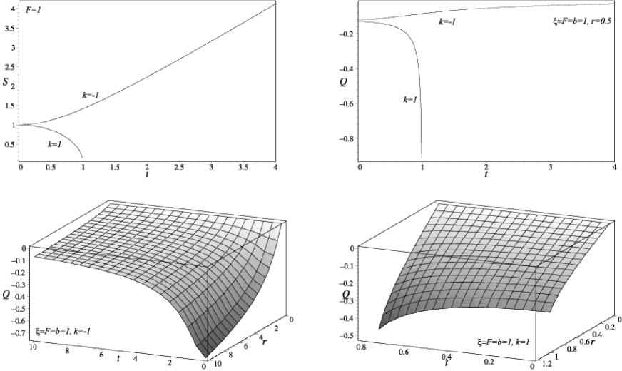
Figure 3: Scale factor and the function $Q$ (which governs the Weyl 1-form) in case of the intermediate solution, i.e. $\Lambda=\chi=0$.

5 Radiative solution

Let us now investigate the branch $\chi\neq 0$, i.e. the induced cosmological constant $\Lambda$ is forced to vanish because of (59). The remaining two field equations (58) and (60) turn into

$$\frac{\ddot{S}}{S}+\left(\frac{\dot{S}}{S}\right)^{2}+\frac{k}{S^{2}} = 0,$$ (78)

$$\chi\frac{\ddot{S}}{S}+\frac{\kappa\mu_{0}}{3S^{4}} = 0.$$ (79)

This set is solved by

$$S(t) =\sqrt{\frac{\kappa\mu_{0}}{3k\chi}-kt^{2}}\quad\quad \texttt{\rm for }k=-1,1\,,$$ (80)

$$S(t) =\sqrt{C+2\sqrt{\frac{\kappa\mu_{0}}{3\chi}}t}\quad\quad \texttt{\rm for }k=0.$$ (81)

Here $C$ denotes an arbitrary constant. Again, we derive the effective energy and pressures (48):

$${}^{{\rm rad}}\tilde{\mu}:= \,{}^{{\rm rad}}\mu-\,^{{\rm vac}}\mu=\frac{\mu_{0}}{S^{4}},\quad$$ (82)

$${}^{{\rm rad}}\tilde{p}_{r}:= \,{}^{{\rm rad}}p_{r}-\,^{{\rm vac}}p_{r}=\frac{\mu_{0}}{3S^{4}},\quad^{{\rm rad}}\tilde{p}_{t}:=\,^{{\rm rad}}p_{t}-\,^{{\rm vac}}p_{t}=\frac{\mu_{0}}{3S^{4}}.$$ (83)

Thus, with $\,{}^{{\rm rad}}\tilde{p}:=\,^{{\rm rad}}\tilde{p}_{r}=\,^{{\rm rad}}\tilde{p}_{t}$, the radiative relation between the effective energy and pressure holds:

$${}^{{\rm rad}}\tilde{p}=\frac{{}^{{\rm rad}}\tilde{\mu}}{3}\,.$$ (84)

Finally, the Weyl 1-form reads

$$Q =-\frac{\xi(t)}{4b\sqrt{t^{2}-\frac{\kappa\mu_{0}}{3\chi}}}\,\texttt{\rm arcsinh}(r)\,\vartheta^{\hat{0}}\quad\quad \texttt{\rm for }k=-1,$$ (85)

$$Q =-\frac{\xi(t)\,r}{4b\sqrt{C+2\sqrt{\frac{\kappa\mu_{0}}{3\chi}}t}}\,\vartheta^{\hat{0}}\quad\quad \texttt{\rm for }k=0,$$ (86)

$$Q =-\frac{\xi(t)}{4b\sqrt{\frac{\kappa\mu_{0}}{3\chi}-t^{2}}}\,\texttt{\rm arcsin}(r)\,\vartheta^{\hat{0}}\quad\quad \texttt{\rm for }k=1.$$ (87)

Again, we observe that the only surviving pieces of the curvature are ${}^{(4)}W_{\alpha\beta}\,$ and ${}^{(4)}Z_{\alpha\beta}$, their nonvanishing components are given by:

$${}^{(4)}Z_{\hat{0}\hat{0}} =\frac{3\chi k\xi(t)}{8b\left(3\chi t^{2}-\kappa\mu_{0}\right)}\,\vartheta^{\hat{0}}\wedge\vartheta^{\hat{1}}$$ (88)

$$=-\,^{(4)}Z_{\hat{1}\hat{1}}=-\,^{(4)}Z_{\hat{2}\hat{2}}=-\,^{(4)}Z_{\hat{3}\hat{3}}\, \texttt{\rm for }k=1,-1,$$

$${}^{(4)}Z_{\hat{0}\hat{0}} =\frac{\xi(t)}{8b\left(2\sqrt{\frac{\kappa\mu_{0}}{3\chi}}t+C\right)}\,\vartheta^{\hat{0}}\wedge\vartheta^{\hat{1}}$$ (89)

$$=-\,^{(4)}Z_{\hat{1}\hat{1}}=-\,^{(4)}Z_{\hat{2}\hat{2}}=-\,^{(4)}Z_{\hat{3}\hat{3}}\, \texttt{\rm for }k=0,$$

$${}^{(4)}W^{\alpha\beta} =\frac{3\chi\kappa\mu_{0}}{\left(3\chi t^{2}-\mu_{0}\kappa\right)^{2}}\vartheta^{\alpha}\wedge\vartheta^{\beta}\,\quad \texttt{\rm for }k=-1,1\,,$$ (90)

$${}^{(4)}W^{\alpha\beta} =\frac{\kappa\mu_{0}}{12\sqrt{\frac{\kappa\mu_{0}}{3\chi}}\chi Ct+3\chi C^{2}+4\kappa\mu_{0}t^{2}}\,\vartheta^{\alpha}\wedge\vartheta^{\beta}\quad \texttt{\rm for }k=0.$$ (91)

In table 4 we list the parameter values and epochs at which the curvature invariant diverges.

Table 4: Parameter and times with essential singularities (radiative solution).

• $k=-1$	$\{b=0\}\,\,$or$\,\,\,\{t_{{\rm div}}=\pm\sqrt{\frac{\mu_{0}\kappa}{3\chi}}\}$ or $\{\kappa=0,\,\chi=0\}\,$ or $\{t=0,\,\kappa=0\}$
  $k=0$	$\{b=0\}$ or$\,\,\,\{t_{{\rm div}}=-\frac{C}{2}\sqrt{\frac{3\chi}{\kappa\mu_{0}}}\}$
  $k=1$	$\{b=0\}\,\,$or$\,\,\,\{t_{{\rm div}}=\pm\sqrt{\frac{\mu_{0}\kappa}{3\chi}}\}$ or $\{\kappa=0,\,\chi=0\}\,$ or $\{t=0,\,\kappa=0\}$

The situation is the same as in case of the vacuum and intermediate solution, i.e. the times $t_{{\rm div}}$ correspond to $S(t_{{\rm div}})=0$, yielding a point singularity at the origin of the universe.

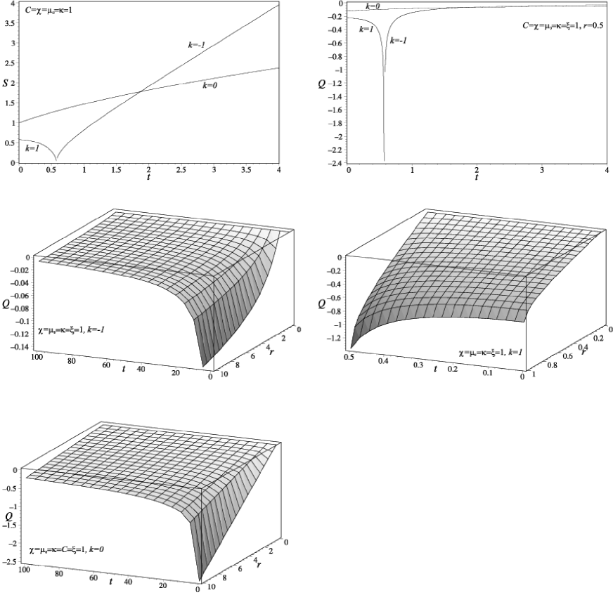
Figure 4: Scale factor $S$ and the function $Q$ (which governs the Weyl 1-form) in case of the radiative ($\Lambda=0$, $\chi\neq 0$) solution.

6 Conclusion

We were able to recover the results found in [6]. We fixed some dimensional problems and calculated the explicit form of the curvature pieces for all branches of the solution. From the figures 2–4 we gain insight into the behavior of the Weyl 1-from $Q$ which controls the non-Riemannian features of the solution. Since we expect that the non-Riemannian quantities are only present at very early stages of the universe, the explicit form of $Q$ (cf. eqs. (64)-(66), (74)-(75), (85)-(87)) restricts the allowed choices for the function $\xi(t)$ entering our ansatz in (24). Thus, in case of a suitable choice for $\xi(t)$, the solution asymptotically evolves from a Weyl-Cartan into a Riemannian spacetime. We note that some of the previously found branches of the solution can be matched. For this purpose, we investigate the $k=-1$ branch. The corresponding scale factors are listed in table 5.

Table 5: Comparison of the scale factors in case of $k=-1$ for all branches.

• 	Vacuum	Intermediate	Radiative
  Parameters	$\Lambda\neq 0,\chi=0$	$\Lambda=0,\chi=0$	$\Lambda=0,\chi\neq 0$
  Scale factors	$S(t)=A\,e^{\sqrt{\frac{\Lambda}{3}}t}-\frac{3}{4A\Lambda}\,e^{-\sqrt{\frac{\Lambda}{3}}t}$	$S(t)=\sqrt{F+\,t^{2}}$	$S(t)=\sqrt{t^{2}-\frac{\kappa\mu_{0}}{3\chi}}$

From this table it is clear that the intermediate and radiative scale factors can be matched by choosing $F=-\frac{\kappa\mu_{0}}{3\chi}$.

In figure 5 we display all three branches in one plot. With the exception of $t$, we set all free parameters to the value $1$.

Figure 5: Scale factors for all three branches of the solution, i.e. the vacuum ($\Lambda\neq 0$, $\chi=0$), intermediate ($\Lambda=\chi=0$), and radiative ($\Lambda=0$, $\chi\neq 0$) part.

Finally, we note that the singularities of the solution are of the same type as in the Riemannian case, i.e. point singularities at the origin of the universe. This result is rather surprising, because most of the known extensions of the cosmological standard model exhibit singularities of extended geometrical shape (cf. [2], [9]) or, in some cases, lead to the avoidance of a singularity (cf. [10]). In future work it might be interesting to incorporate anisotropic and inhomogeneous metrical structures into our model.

Appendix A MAG in general

In MAG we have the metric $g_{\alpha\beta}$, the coframe $\vartheta^{\alpha}$, and the connection 1-form $\Gamma_{\alpha}{}^{\beta}$ (with values in the Lie algebra of the four-dimensional linear group $GL(4,R)$) as new independent field variables. Here $\alpha,\beta,\ldots=0,1,2,3$ denote (anholonomic) frame indices. Spacetime is described by a metric-affine geometry with the gravitational field strengths nonmetricity $Q_{\alpha\beta}:=-Dg_{\alpha\beta}$, torsion $T^{\alpha}:=D\vartheta^{\alpha}$, and curvature $R_{\alpha}{}^{\beta}:=d\Gamma_{\alpha}{}^{\beta}-\Gamma_{\alpha}\,^{\gamma}\wedge\Gamma_{\gamma}{}^{\beta}$. A Lagrangian formalism for a matter field $\Psi$ minimally coupled to the gravitational potentials $g_{\alpha\beta}$, $\vartheta^{\alpha}$, $\Gamma_{\alpha}{}^{\beta}$ has been set up in [3]. An alternative interpretation of the metric as a Goldstone field, no more playing the role of a fundamental gravitational potential, has been proposed by Mielke and one of the authors in [7] in the context of nonlinear realizations of spacetime groups. The dynamics of an ordinary MAG theory is specified by a total Lagrangian

$$L=V_{{\rm MAG}}(g_{\alpha\beta},\vartheta^{\alpha},Q_{\alpha\beta},T^{\alpha},R_{\alpha}{}^{\beta})+L_{{\rm mat}}(g_{\alpha\beta},\vartheta^{\alpha},\Psi,D\Psi).$$ (92)

The variation of the action with respect to the independent gauge potentials leads to the field equations:

$$\frac{\delta L_{{\rm mat}}}{\delta\Psi} = 0,$$ (93)

$$DM^{\alpha\beta}-m^{\alpha\beta} = \sigma^{\alpha\beta},$$ (94)

$$DH_{\alpha}-E_{\alpha} = \Sigma_{\alpha,}$$ (95)

$$DH^{\alpha}{}_{\beta}-E^{\alpha}{}_{\beta} = \Delta^{\alpha}{}_{\beta}.$$ (96)

Equation (95) is the generalized Einstein equation with the energy-momentum 3-form $\Sigma_{\alpha}$ as its source, whereas (94) and (96) are additional field equations which take into account other aspects of matter, such as spin, shear and dilation currents, represented by the hypermomentum $\Delta^{\alpha}{}_{\beta}$. We made use of the definitions of the gauge field excitations,

$$H_{\alpha}:=-\frac{\partial V_{{\rm MAG}}}{\partial T^{\alpha}},\quad H^{\alpha}{}_{\beta}:=-\frac{\partial V_{{\rm MAG}}}{\partial R_{\alpha}{}^{\beta}},\quad M^{\alpha\beta}:=-2\frac{\partial V_{{\rm MAG}}}{\partial Q_{\alpha\beta}},$$ (97)

of the canonical energy-momentum, the metric stress-energy and the hypermomentum current of the gauge fields,

$$E_{\alpha}:=\frac{\partial V_{{\rm MAG}}}{\partial\vartheta^{\alpha}},\quad m^{\alpha\beta}:=2\frac{\partial V_{{\rm MAG}}}{\partial g_{\alpha\beta}},\quad E^{\alpha}{}_{\beta}:=-\vartheta^{\alpha}\wedge H_{\beta}-g_{\beta\gamma}M^{\alpha\gamma},$$ (98)

and of the canonical energy-momentum, the metric stress-energy and the hypermomentum currents of the matter fields,

$$\Sigma_{\alpha}:=\frac{\delta L_{{\rm mat}}}{\delta\vartheta^{\alpha}},\quad\sigma^{\alpha\beta}:=2\frac{\delta L_{{\rm mat}}}{\delta g_{\alpha\beta}},\quad\Delta^{\alpha}{}_{\beta}:=\frac{\delta L_{{\rm mat}}}{\delta\Gamma_{\alpha}{}^{\beta}}.$$ (99)

Provided the matter equations (93) are fulfilled, the following Noether identities hold:

$$D\Sigma_{\alpha} = \left(e_{\alpha}\rfloor T^{\beta}\right)\wedge\Sigma_{\beta}-\frac{1}{2}\left(e_{\alpha}\rfloor Q_{\beta\gamma}\right)\sigma^{\beta\gamma}+\left(e_{\alpha}\rfloor R_{\beta}{}^{\gamma}\right)\wedge\Delta^{\beta}{}_{\gamma},$$ (100)

$$D\Delta^{\alpha}{}_{\beta} = g_{\beta\gamma}\sigma^{\alpha\gamma}-\vartheta^{\alpha}\wedge\Sigma_{\beta}.$$ (101)

They show that the field equation (94) is redundant, thus we only need to take into account (95) and (96).

As suggested in [3], the most general parity conserving quadratic Lagrangian expressed in terms of the irreducible pieces of the nonmetricity $Q_{\alpha\beta}$, torsion $T^{\alpha}$, and curvature $R_{\alpha\beta}$ reads

$$V_{{\rm MAG}}= \frac{1}{2\kappa}\biggl{[} -a_{0}R^{\alpha\beta}\wedge\eta_{\alpha\beta}-2\lambda\eta+T^{\alpha}\wedge\,^{\star}\left(\sum_{I=1}^{3}a_{I}\,^{(I)}T_{\alpha}\right)$$

$$+Q_{\alpha\beta}\wedge\,^{\star}\left(\sum_{I=1}^{4}b_{I}\,^{(I)}Q^{\alpha\beta}\right)$$

$$+b_{5}\left({}^{(3)}Q_{\alpha\gamma}\wedge\vartheta^{\alpha}\right)\wedge\,^{\star}\left(\,{}^{(4)}Q^{\beta\gamma}\wedge\vartheta_{\beta}\,\right)$$

$$+2\left(\sum_{I=2}^{4}c_{I}\,^{(I)}Q_{\alpha\beta}\right)\wedge\vartheta^{\alpha}\wedge\,^{\star}T^{\beta}\biggr{]}$$

$$-\frac{1}{2\rho}\,R^{\alpha\beta}\wedge\,^{\star} \biggl{[}\sum_{I=1}^{6}w_{I}\,^{(I)}W_{\alpha\beta}+\sum_{I=1}^{5}z_{I}\,^{(I)}Z_{\alpha\beta}+w_{7}\vartheta_{\alpha}\wedge\left(e_{\gamma}\rfloor\,^{(5)}W^{\gamma}{}_{\beta}\right)$$ (102)

$$+z_{6}\vartheta_{\gamma}\wedge\left(e_{\alpha}\rfloor\,^{(2)}Z^{\gamma}{}_{\beta}\right)+\sum_{I=7}^{9}z_{I}\vartheta_{\alpha}\wedge\left(e_{\gamma}\rfloor\,^{(I-4)}Z^{\gamma}{}_{\beta}\right)\biggr{]}.$$

The constants entering (102) are the cosmological constant $\lambda$, the weak and strong coupling constant $\kappa$ and $\rho$, and the 28 dimensionless parameters

$$a_{0},\dots,a_{3},b_{1},\dots,b_{5},c_{2},\dots,c_{4},w_{1},\dots,w_{7},z_{1},\dots,z_{9}.$$ (103)

This Lagrangian and the presently known exact solutions in MAG have been reviewed in [5]. We note that this Lagrangian incorporates the one used in section 2 eq. (2), as can be seen easily by making the following choice for the constants in (102):

$$\lambda,a_{1},\dots,a_{3},b_{1},\dots,b_{5},c_{2},\dots,c_{4},w_{7},z_{1},\dots,z_{3},z_{5},\dots,z_{9}=0.\quad$$ (104)

In order to obtain exactly the form of (2), one has to perform the additional substitutions:

$$a_{0}\rightarrow-\chi,\quad w_{1},\dots,w_{6}\rightarrow-2\rho a_{1},\dots,-2\rho a_{6},\quad z_{4}\rightarrow-2\rho b.$$ (105)

Appendix B Weyl-Cartan spacetime

The Weyl-Cartan  spacetime ($Y_{n}$) is a special case of the general metric-affine geometry in which the tracefree part $Q_{\alpha\beta}\!\!\!\!\!\!\!\!\!\!\!\!\!\nearrow\,\,\,\,\,\,\,$ of the nonmetricity $Q_{\alpha\beta}\,$ vanishes. Thus, the whole nonmetricity is proportional to its trace part, i.e. the Weyl 1-form $Q:=\frac{1}{4}Q^{\alpha}{}_{\alpha}$,

$$Q_{\alpha\beta}=g_{\alpha\beta}\,Q=\frac{1}{4}g_{\alpha\beta}\,Q^{\gamma}{}_{\gamma}.$$ (106)

Therefore the general MAG connection reduces to

$$\Gamma_{\alpha\beta} = \frac{1}{2}dg_{\alpha\beta}+\left(e_{[\alpha}\rfloor dg_{\beta]\gamma}\right)\vartheta^{\gamma}+e_{[\alpha}\rfloor C_{\beta]}-\frac{1}{2}\left(e_{\alpha}\rfloor e_{\beta}\rfloor C_{\gamma}\right)\vartheta^{\gamma}$$ (107)

$$-e_{[\alpha}\rfloor T_{\beta]}+\frac{1}{2}\left(e_{\alpha}\rfloor e_{\beta}\rfloor T_{\gamma}\right)\vartheta^{\gamma}+\frac{1}{2}g_{\alpha\beta}\,Q+\left(e_{[\alpha}\rfloor Q\right)\vartheta_{\beta]}$$

$$= \Gamma_{\alpha\beta}^{\{\,\}}-e_{[\alpha}\rfloor T_{\beta]}+\frac{1}{2}\left(e_{\alpha}\rfloor e_{\beta}\rfloor T_{\gamma}\right)\vartheta^{\gamma}+\frac{1}{2}g_{\alpha\beta}\,Q+\left(e_{[\alpha}\rfloor Q\right)\vartheta_{\beta]}.$$ (108)

Thus, it not longer includes a symmetric tracefree part. Now let us recall the definition of the material hypermomentum $\Delta_{\alpha\beta}$ given in (99). Due to the absence of a symmetric tracefree piece in (108), $\Delta_{\alpha\beta}$ decomposes as follows

$$\Delta_{\alpha\beta} =$$ antisymmetric piece + trace piece (109)

$$= \tau_{\alpha\beta}+\frac{1}{4}g_{\alpha\beta}\,\Delta=\tau_{\alpha\beta}+\frac{1}{4}g_{\alpha\beta}\,\Delta^{\gamma}{}_{\gamma}$$

$$=$$ spin current + dilation current.

According to (109) the second MAG field equation (96) decomposes into

$$dH^{\alpha}{}_{\alpha}-E^{\alpha}{}_{\alpha} = \Delta,$$ (110)

$$g_{\gamma[\alpha}DH^{\gamma}\,_{\beta]}-E_{[\alpha\beta]} = \tau_{\alpha\beta},$$ (111)

while the first field equation is still given by (95). Additionally, we can decompose the second Noether identity (101) into

$$\frac{1}{4}g_{\alpha\beta}\,d\Delta+\vartheta_{(\alpha}\wedge\Sigma_{\beta)} = \sigma_{\alpha\beta},$$ (112)

$$D\tau_{\alpha\beta}+Q\wedge\tau_{\alpha\beta}+\vartheta_{[\alpha}\wedge\Sigma_{\beta]} = 0.$$ (113)

Thus, the first Noether identity (100) with inserted Weyl 1-form and hypermomentum reads

$$D\Sigma_{\alpha}=\left(e_{\alpha}\rfloor T^{\beta}\right)\wedge\Sigma_{\beta}-\frac{1}{2}\left(e_{\alpha}\rfloor Q\right)\sigma^{\beta}{}_{\beta}+\left(e_{\alpha}\rfloor R_{[\beta\gamma]}{}\right)\wedge\tau^{\beta\gamma}+\frac{1}{4}\left(e_{\alpha}\rfloor R\right)\wedge\Delta.$$ (114)

Finally, we note that in a $Y_{n}$ spacetime the symmetric part of the curvature $R_{(\alpha\beta)}=Z_{\alpha\beta}\,$, i.e. the strain curvature, reduces to the trace part

$$Z_{\alpha\beta}=\frac{1}{4}g_{\alpha\beta}R=\frac{1}{4}g_{\alpha\beta}R^{\gamma}{}_{\gamma}=\frac{1}{2}g_{\alpha\beta}\,dQ.$$ (115)

Appendix C Units

In this work we made use of natural units, i.e. $\hbar=c=1$ (cf. table 6).

Table 6: Natural units.

• [energy]	[mass]	[time]	[length]
  length-1	length-1	length	length

Additionally, we have to be careful with the coupling constants and the coordinates within the coframe. In order to keep things as clear as possible, we provide a list of the quantities emerging in section 2 in table 7.

Table 7: Units of quantities in section 2.

• Quantities	Units
  Coordinates	$[t]=$ length, $[\phi]=[r]=[\theta]=1$
  Constants	$[k]=[\chi]=[b]=1,$ $[\Lambda]^{-\frac{1}{2}}=[\kappa]^{\frac{1}{2}}=$ length
  Functions	$[S(t)]=$ length, $[\xi(t)]=1$
  Additional constants	$[A]=[F]^{\frac{1}{2}}=[C]^{\frac{1}{2}}=$ length, $[\mu_{0}]=1$

Note that $[d]=1$ and $[\,^{\star}]=$ length^n-2p, where $n=$ dimension of the spacetime, $p=$ degree of the differential form on which ^⋆ acts.

References

- [1] E.W. Kolb, Michael S. Turner: The early universe. Addison-Wesley (1990)
- [2] G. Börner: The early universe - Facts and fiction. Springer, 3rd edition (1993)
- [3] F.W. Hehl, J.D. McCrea, E.W. Mielke, Y. Ne´eman: Metric-affine gauge theory of gravity: Field equations, Noether identities, world spinors, and breaking of dilation invariance. Phys. Rep. 258 (1995) 1-171
- [4] J.D. McCrea: Irreducible decompositions of the non-metricity, torsion, curvature and Bianchi identities in metric-affine spacetimes. Class. Quantum Grav. 9 (1992) 553-568
- [5] F.W. Hehl, A. Macías: Metric-affine gauge theory of gravity: II. Exact solutions. Int. J. Mod. Phys. D, Vol.8, No. 4 (1999) 399-416
- [6] R. Tresguerres: Weyl-Cartan model for cosmology before mass generation. Proc. Relativity in general, Salas, Asturias, (Spain), Sept. 7-10 (1993) Eds. J. Diaz Alonso, M. Lorente Paramo 407-413
- [7] R. Tresguerres, E.W. Mielke: Gravitational Goldstone fields from affine gauge theory. Phys. Rev. D 62 (2000) 044004
- [8] Y.N. Obukhov, R. Tresguerres: Hyperfluid - a model of classical matter with hypermomentum. Phys. Lett. A 184 (1993) 17-22
- [9] M.A.H. MacCallum: Cosmological models from a geometric point of view. Cargèse Lectures in Physics (1971) Ed. E. Schatzman 61-174
- [10] R.W. Tucker, C. Wang: Dark matter gravitational interactions Class. Quantum Grav. 15 (1998) 933-954