BA-TH/00-402 gr-qc/0101019  
Gravitational waves in non-singular string cosmologies

Abstract

We study the evolution of tensor metric fluctuations in a class of non-singular models based on the string effective action, by including in the perturbation equation the higher-derivative and loop corrections needed to regularise the background solutions. We discuss the effects of such higher-order corrections on the final graviton spectrum, and we compare the results of analytical and numerical computations.

1 Introduction

Recent studies, including strong coupling corrections to the string effective action, have provided the pre-Big Bang scenario [1, 2] with a number of promising models for the transition from the growing to the decreasing curvature regime [3, 4, 5, 6]. However, a crucial question remains: is it possible to test this cosmological scenario and, in particular, to distinguish it from other, more conventional descriptions of the very early Universe?

The answer to this essential question is in principle positive, since the pre-Big Bang scenario incorporates a dilaton field which modifies the standard inflationary kinematics and which, through its non-minimal coupling, also directly modifies the evolution of perturbations (of the metric, and of the other background fields) [7]. It is well known, on the other hand, that the transition from an inflationary period to the usual Friedman-Robertson-Walker (FRW) phase amplifies tensor metric perturbations, and is associated with the production of a stochastic background of relic gravitational waves [8, 9].

Such a primordial background decouples from matter immediately below the Planck scale, unlike the electromagnetic radiation which underwent a complicated history until recombination, and has been transmitted almost unperturbed down to our present epoch. As a consequence, its present spectrum should be a faithful portrait of the very early universe [10], thus opening a window for the observation of processes occurring near to the Planck scale, and for discriminating among various models of primordial evolution.

In the context of string cosmology, several mechanisms may contribute to the generation of gravitational waves from the initial vacuum state. One contribution comes from the process of dynamical dimensional reduction [11, 12, 13], when the internal dimensions shrink down to a final compactification scale. Another contribution is due to the time-dependence of the dilaton field – and thus of the effective gravitational coupling constant – during the pre-Big Bang phase [14, 15]. Finally, there is the usual contribution arising from the accelerated expansion of the external three-dimensional space. Both the dilaton and the full, higher-dimensional metric thus contribute to the external “pump” field which is responsible for the parametric amplification of tensor metric fluctuations, normalised to an initial vacuum fluctuation spectrum.

With respect to the standard inflationary scenario, the amplification of tensor perturbations in the pre-Big Bang scenario is strongly enhanced for large comoving wavenumber $k$ [16, 14], in such a way that the produced background of gravitational waves could in principle be detected in the near future by various planned experiments [2, 16, 17]. Arguments in favour of this conclusion arise from the particular kinematics of string cosmology. First, since the Hubble parameter is increasing in the pre-Big Bang phase, higher frequency modes will cross the horizon at higher values of $|H|$, which implies that the amplitude of the spectrum increases with frequency. In this context, the comoving amplitude of perturbations may grow even outside the horizon [18, 19, 20], instead of being frozen as happens in standard inflation. Second, the peak amplitude of the spectrum (naturally located in the high frequency regime, near the end point of the spectrum) is normalised so as to match the string scale [17, 21], i.e. nearly eight orders of magnitude above the high frequency normalisation of the standard scenario [22]. Hence, the pre-Big Bang phase could lead to a very efficient production of gravitons in the sensitivity range of present gravitational antenna. In fact such a relic background could be in principle be detected by the second (planned) generation of interferometric detectors [23, 24].

To date, extended studies of tensor perturbations have been mostly performed in the context of the tree-level effective action, with and without the possible contribution of a high curvature stringy phase. In all cases the background cosmologies that have been investigated have been singular, i.e. the curvature and dilaton have become singular at some fixed proper time. There have been a number of suggested ways to tackle the singularity problem, considering also anisotropic [25, 26] and inhomogeneous [27, 28] backgrounds, or the presence of a non-local dilaton potential [2]. However, if we confine our attention to homogeneous and isotropic metrics, and to a local potential, one of the most promising approaches to the graceful exit problem [29] suggests that the curvature singularities may be cured by adding higher-order corrections to the string effective action (see for instance [30, 31, 32, 3, 4, 6]). These include both higher-derivative $\alpha^{\prime}$ corrections, due to finite-size effects, and quantum corrections, due to the loop expansion in the string coupling parameter. In the context of cosmological perturbation theory, it is known [33] that such corrections may induce an additional amplification when the curvature becomes large in string units. The aim of this paper, therefore, is to discuss the evolution and the spectrum of tensor perturbations in the context of a class of non-singular cosmological backgrounds, by taking into account (in the perturbation equation) the full contribution of those corrections that are responsible for the regularisation of the background evolution. In this way it will be possible (for the first time, to the best of our knowledge) to follow the complete evolution of perturbations, from the initial vacuum down to the present time, through a continuous numerical integration of the linearised perturbation equations.

The paper is organised as follows. In Section 2 we recall the general form of the first order $\alpha^{\prime}$ corrections arising in the context of the massless bosonic sector of the low-energy heterotic string action. We extend them by including possible one- and two-loop quantum corrections, and we write down the corresponding background equations. In Section 3 we compute the linearised tensor perturbation equation, including such higher-order corrections. In Section 4 we present a general discussion of the evolution of perturbations in the presence of higher-order curvature corrections. We then check the main points of our discussion through a numerical integration of the perturbation equations for regular backgrounds, by using an appropriate dilaton potential, or particle production effects, to stabilise the dilaton in the post-Big Bang era. We find that the general effect of the higher-order corrections is to flatten the slope of the high-frequency part of the spectrum, but the effect is probably too small – in the class of models discussed in this paper – to make the graviton background “visible” to the planned advanced detectors. The main results of this paper are finally summarised in Section 5.

2 Effective action and background equations

In the context of the pre-Big Bang scenario, our present FRW Universe is expected to emerge from the string perturbative vacuum as a consequence of some process – for instance, plane wave collisions [34] – triggering the gravitational collapse of a sufficiently large portion of spacetime [35]. The initial evolution is driven by the kinetic energy of the dilaton, and can be described, in the string frame, as inflationary expansion with growing coupling and curvature. After reaching a maximal scale controlled by the fundamental string length $\lambda_{S}$, $|H|\sim{\cal O}(\lambda_{S}^{-1})$, it is then expected that the Universe is smoothly connected to the FRW regime, with a constant dilaton field.

In the early stage of the dilaton-driven inflationary (DDI) period, strings are propagating in a background of small curvature, and the fields are weakly coupled, so that the cosmological evolution is consistently described by the lowest order string effective action which, by assuming static internal dimensions, can be written as:

$$\Gamma=\frac{1}{\alpha^{\prime}}\int d^{4}x\sqrt{-g}\left\{e^{-\phi}\left[R+(\partial_{\mu}\phi)^{2}\right]+{\cal L}_{c}\right\}.$$ (1)

Here $\alpha^{\prime}=\lambda_{S}^{2}$, we have adopted the convention $(-,+,+,+)$, $R^{\mu}_{\;\nu\lambda\rho}=\partial_{\rho}\Gamma^{\mu}_{\nu\lambda}+\dots$, $R_{\nu\rho}=R^{\lambda}_{\;\nu\lambda\rho}$ and set our units such that $\hbar=c=16\pi G=1$. Following [3], we have introduced an additional lagrangian ${\cal L}_{c}$ allowing for the inclusion of higher-order corrections to the tree-level effective action, a non-perturbative potential – yet to be determined – and/or the backreaction of the produced radiation. Considering this additional lagrangian as an independent source we shall assume that the associated energy-momentum tensor is diagonal, homogeneous and isotropic, and can be written in the perfect fluid form as $T^{\mu}_{\nu}={\rm diag}(-\rho_{c},p_{c},p_{c},p_{c})$.

The resulting equations of motion for the background are obtained from the variation of Eq. (1) with respect to the metric and the dilaton field:

$$6H^{2}-6H\dot{\phi}+\dot{\phi}^{2} = e^{\phi}\rho_{c},$$ (2)

$$4\dot{\phi}H-4\dot{H}-6H^{2}-\dot{\phi}^{2}+2\ddot{\phi} = e^{\phi}p_{c},$$ (3)

$$6\dot{H}+12H^{2}+\dot{\phi}^{2}-2\ddot{\phi}-6\dot{\phi}H = e^{\phi}\Delta_{\phi},$$ (4)

$$\dot{\rho_{c}}+3H(\rho_{c}+p_{c}) = -\Delta_{\phi}\dot{\phi}.$$ (5)

A dot represents the differentiation with respect to proper time $t$ and $H=\dot{a}/a$ is the Hubble parameter. $\Delta_{\phi}$ arises from the variation of the additional lagrangian with respect to $\phi$. Finally, Eq. (5) is the conservation equation, a direct consequence of Eq. (2)–Eq. (4).

To lowest order, the homogeneous and isotropic version of the pre-Big Bang scenario, without non-local dilaton potential, inevitably faces a curvature and dilaton singularity at the end of the DDI phase. However, a singular behaviour is often a late manifestation of the breakdown of the description, extended beyond its domain of validity. Hence, the low-energy dynamics should be supplemented by corrections, in order to give a reliable description of the high curvature regime, expected to be crossed before reaching the FRW universe. Such corrections are generally of two types: tree-level $\alpha^{\prime}$ corrections, referring to the finite size of the string, and quantum corrections, resulting from a more conventional loop expansion in the string coupling parameter.

It has been shown in [32] that the higher curvature $\alpha^{\prime}$ terms, arising from the expansion around the point-particle limit, may eventually stabilise the evolution of the Universe into a de-Sitter like regime of constant curvature $H\sim{\cal O}(\lambda^{-1}_{S})$ and linearly growing (in cosmic time) dilaton. In this paper we will consider the most general tree-level $\alpha^{\prime}$ corrections to the gravi-dilaton string action up to fourth-order in derivatives (see [6] for a detailed analysis), which can be written in the form [36]:

$${\cal L}_{\alpha^{\prime}}=\alpha^{\prime}\lambda_{0}e^{-\phi}\left\{c_{1}R^{2}_{GB}+c_{2}G^{\mu\nu}\partial_{\mu}\phi\partial_{\nu}\phi+c_{3}\Box\phi(\partial_{\mu}\phi)^{2}+c_{4}(\partial_{\mu}\phi)^{4}\right\},$$ (6)

$$c_{1}=-1,\hskip 28.45274ptc_{2}+2(c_{3}+c_{4})=-2c_{1}.$$ (7)

The constraint Eq. (7) on the coefficients is required so that the action reproduces the usual string scattering amplitudes [36]. The parameter $\lambda_{0}$ allows us to move between different string models, and we will later use $\lambda_{0}=-1/4$ to agree with previous studies of the heterotic string [32]. Finally, $R^{2}_{GB}=R_{\mu\nu\lambda\rho}R^{\mu\nu\lambda\rho}-4R_{\mu\nu}R^{\mu\nu}+R^{2}$ is the Gauss-Bonnet combination, guaranteeing the absence of derivatives higher than two in the equations of motion.

Another conventional expansion of the string effective action is controlled by the string coupling parameter, $g^{2}_{string}=e^{\phi}$. Initially, $g^{2}_{string}\ll 1$. However, the growth of the dilaton during the DDI era implies that the late evolution of the background could be dominated by quantum loop corrections, which will eventually force the universe to escape from the fixed point determined by the $\alpha^{\prime}$ corrections [32], for a smooth connection to the post-Big Bang regime. Unfortunately, there is as yet no definitive calculation of the full loop expansion in string theory, so we are left to speculate on plausible terms that will eventually make up the loop contribution. Multiplying each term of the tree-level $\alpha^{\prime}$ correction by a suitable power of the string coupling is the approach which has already met with some success [3, 5, 6], and which we shall adopt also in this paper. Since the quantum corrections are not formally derived from an explicit computation, we shall allow for different coefficients $d_{i}$ ($e_{i}$) at one-loop (two-loop) in the string coupling, replacing the coefficients $c_{i}$ of the tree-level action, where $d_{i}$ and $e_{i}$ are not necessarily subject to the constraint Eq. (7). With such assumptions, the effective lagrangian density ${\cal L}_{c}$ of Eq. (1), which is in general the sum of the tree-level $\alpha^{\prime}$ and loop corrections, ${\cal L}_{c}={\cal L}_{\alpha^{\prime}}+{\cal L}_{g}$, in the present case will take the form

$${\cal L}_{c}={\cal L}_{\alpha^{\prime}}(c_{i})+Ae^{\phi}{\cal L}_{\alpha^{\prime}}(d_{i})+Be^{2\phi}{\cal L}_{\alpha^{\prime}}(e_{i}),$$ (8)

where ${\cal L}_{\alpha^{\prime}}(c_{i})$ is given by Eq. (6), with the constant parameters $A$ and $B$ actually controlling the onset of the loop corrections.

The very similarity between the first order $\alpha^{\prime}$ and loop corrections enables a simple form for their contributions to the background equations of motion. From now on, we introduce an additional parameter $n$ in the exponential of the correction ${\cal L}_{c}$, such that $\alpha^{\prime}$ corrections correspond to $n=0$, whereas one- or two-loop corrections correspond to $n=1$ and $n=2$ respectively. For instance, using the notation $\{\dots\}_{1}$ to represent the one-loop contribution ($n=1$ inside the brackets), we easily get the source terms for the system Eq. (2)–Eq. (4):

$$\rho_{c} = \{\rho_{c}\}_{0}+A\{\rho_{c}\}_{1}+B\{\rho_{c}\}_{2},$$ (9)

$$p_{c} = \{p_{c}\}_{0}+A\{p_{c}\}_{1}+B\{p_{c}\}_{2},$$ (10)

$$\Delta_{\phi} = \{\Delta_{\phi}\}_{0}+A\{\Delta_{\phi}\}_{1}+B\{\Delta_{\phi}\}_{2},$$ (11)

and the terms in brackets are given respectively by:

$$\{{\rho}_{c}\}_{n} = \alpha^{\prime}\lambda_{0}\dot{\phi}e^{(n-1)\phi}\Bigl{\{}-24c_{1}(n-1)H^{3}+9c_{2}\dot{\phi}H^{2}+6c_{3}\dot{\phi}^{2}H-\left[c_{3}(n-1)-3c_{4}\right]\dot{\phi}^{3}\Bigr{\}},$$

$$\{p_{c}\}_{n} = \alpha^{\prime}\lambda_{0}e^{(n-1)\phi}\Bigl{\{}\left[8c_{1}(n-1)^{2}-3c_{2}\right]\dot{\phi}^{2}H^{2}-2c_{2}(n-1)\dot{\phi}^{3}H-2c_{3}\dot{\phi}^{2}\ddot{\phi}$$

$$\hskip 59.75095pt+8c_{1}(n-1)\ddot{\phi}H^{2}+16c_{1}(n-1)\dot{\phi}H\left[\dot{H}+H^{2}\right]$$

$$\hskip 59.75095pt-4c_{2}\dot{\phi}\ddot{\phi}H-2c_{2}\dot{\phi}^{2}\dot{H}+\left[c_{4}-c_{3}(n-1)\right]\dot{\phi}^{4}\Bigr{\}},$$

$$\{\Delta_{\phi}\}_{n} = \alpha^{\prime}\lambda_{0}e^{(n-1)\phi}\Bigl{\{}24c_{1}(n-1)H^{2}\left[\dot{H}+H^{2}\right]-3c_{4}\dot{\phi}^{2}\left[4\ddot{\phi}+4\dot{\phi}H+(n-1)\dot{\phi}^{2}\right]$$

$$\hskip 59.75095pt+c_{3}\dot{\phi}\left[(n-1)^{2}\dot{\phi}^{3}+4(n-1)\dot{\phi}\ddot{\phi}-6\dot{\phi}\left(\dot{H}+3H^{2}\right)-12\ddot{\phi}H\right]\Bigr{\}}$$

$$\hskip 59.75095pt-3c_{2}\left[2\ddot{\phi}H^{2}+6\dot{\phi}H^{3}+4\dot{\phi}H\dot{H}+(n-1)\dot{\phi}^{2}H^{2}\right]\Bigr{\}}.$$

Here, of course, for $n=1$ the coefficients $c_{i}$ are replaced by $d_{i}$, while for $n=2$ the $c_{i}$ are replaced by $e_{i}$. Note that for $n=0$, $\lambda_{0}=-1/4$, $c_{4}=-c_{1}=1$, one easily recovers the $\alpha^{\prime}$ corrections used in [32, 33].

In general, the combination of tree-level $\alpha^{\prime}$ and quantum loop corrections does not lead to a fixed value for the dilaton in a finite amount of time. Although a non-perturbative (supersymmetry breaking) potential [37] is expected to stabilise the dilaton, here we shall follow [3] by assuming the dilaton is frozen out by radiation, after the transition to the post-Big Bang regime. To this aim we will introduce “by hand” the presence of radiation, coupled to the dilaton and satisfying the conservation equation

$$\dot{\rho}+4H\rho-\frac{1}{2}\Gamma_{\phi}\dot{\phi}^{2}=0,$$ (12)

where $\Gamma_{\phi}$ represents the decay width of the dilaton.

The solutions of the system of equations Eq. (2) – Eq. (4), including the radiation and the quantum corrections, provide the cosmological gravi-dilaton background in which we will study the propagation of tensor perturbations. We will consider a spatially flat FRW manifold, and we will perturb the above equations keeping the dilaton and all sources fixed, $\delta\phi=0$, $\delta T^{\nu}_{\mu}=0$. To lowest order, the tensor fluctuations will obey the usual string frame perturbation equation [14], including the non-minimal coupling to a time-dependent dilaton. On the other hand, the inclusion of higher-order corrections, needed to regularise the background, will inevitably lead to a modification of such a perturbation equation (see [38, 39, 40, 41] for initial studies taking into account higher curvature contributions to the evolution of perturbations).

3 Tensor perturbations

It is well known that gravitational waves, arising from linearised tensor perturbations, do not couple to pressure and energy density, and hence do not contribute to classical gravitational instabilities. Nevertheless, they are of interest as a specific signature of pre-Big Bang cosmologies since, as stressed in a number of papers [2, 16, 14], the production of high-frequency gravitons is strongly enhanced, in string cosmology, with respect to the standard inflationary scenario. In this study we will restrict our attention to tensor metric perturbations around a $d=3$ spatially flat background, parameterised by the transverse, trace-free variable $h_{\mu\nu}$,

$$g_{\mu\nu}\rightarrow g_{\mu\nu}+h_{\mu\nu}\hskip 28.45274pt\textrm{with}\hskip 14.22636pt\nabla_{\nu}h_{\mu}^{\nu}=0=h_{\mu}^{\mu},$$ (13)

where $\nabla_{\nu}$ denotes covariant differentiation with respect to the background metric. Note also that the indices of $h_{\mu\nu}$ are raised or lowered with the unperturbed metric, $h_{\mu}^{\nu}=g^{\nu\rho}h_{\mu\rho}$.

3.1 Linearised equations

The linear evolution equation for the metric fluctuations can be obtained by perturbing the action Eq. (1) up to terms quadratic in the tensor variable $h_{\mu\nu}$:

$$\delta^{(2)}\Gamma = \frac{1}{\alpha^{\prime}}\int d^{4}x\;e^{-\phi}\left[\delta^{(2)}(\sqrt{-g}R)+\delta^{(2)}(\sqrt{-g}\partial_{\mu}\phi\partial^{\mu}\phi)\right]$$ (14)

$$+\lambda_{0}\int d^{4}x\left[\{\delta^{(2)}{\cal L}\}_{0}+A\{\delta^{(2)}{\cal L}\}_{1}+B\{\delta^{(2)}{\cal L}\}_{2}\right],$$

where the integrand of the $n$-correction is given by:

$$\{\delta^{(2)}{\cal L}\}_{n} = e^{(n-1)\phi}\biggl{\{}\delta^{(2)}(c_{1}\sqrt{-g}R^{2}_{GB})+\delta^{(2)}\left(c_{2}\sqrt{-g}\left[R^{\mu\nu}-\frac{1}{2}g^{\mu\nu}R\right]\partial_{\mu}\phi\partial_{\nu}\phi\right)$$ (15)

$$\hskip 56.9055pt+\delta^{(2)}\left(c_{3}\sqrt{-g}\Box\phi(\partial_{\mu}\phi)^{2}\right)+\delta^{(2)}\left(c_{4}\sqrt{-g}(\partial_{\mu}\phi)^{4}\right)\biggr{\}}.$$

Following [33], it is convenient to use the synchronous gauge where

$$g_{00}=-1, ~{}~{}g_{0i}=0,~{}~{} ~{}~{}g_{ij}=a^{2}\delta_{ij},$$

$$h_{00}=0,\hskip 8.5359pt ~{}~{}h_{0i}=0,~{}~{} g^{ij}h_{ij}=0\hskip 14.22636pt\textrm{and}\hskip 14.22636pt\partial_{j}h^{j}_{\;i}=0.$$ (16)

This enables us to write the perturbed action as a quadratic form depending on the first and second derivatives of the symmetric, trace-free matrix $h=h^{i}_{\;j}$, with time-dependent coefficients fixed by the background fields $a(t)$, $\phi(t)$. Introducing the matrix notation $\textrm{Tr}\;h^{2}\equiv h_{i}^{\;j}h_{j}^{\;i}$, and using $\nabla^{2}=\delta^{ij}\partial_{i}\partial_{j}$ for the Laplace operator in a flat space, we have

$$\delta^{(2)}\Gamma = \frac{1}{\alpha^{\prime}}\int d^{4}x\;a^{3}e^{-\phi}\;\textrm{Tr}\;\Biggl{\{}\left[\frac{1}{4}\dot{\phi}^{2}-\frac{3}{2}\dot{H}-3H^{2}\right]h^{2}$$ (17)

$$\hskip 99.58464pt-h\ddot{h}-4Hh\dot{h}-\frac{3}{4}\dot{h}^{2}+\frac{1}{4}h\frac{\nabla^{2}}{a^{2}}h\Biggr{\}}$$

$$+\lambda_{0}\int d^{4}x\;\textrm{Tr}\;\left[\{\otimes\}_{0}+A\{\otimes\}_{1}+B\{\otimes\}_{2}\right],$$

where the integrand of the $n$-correction is given by:

$$\{\otimes\}_{n} = a^{3}e^{(n-1)\phi}\Biggl{\{}\left[-6c_{1}H^{2}\left(\dot{H}+H^{2}\right)-\frac{1}{4}\dot{\phi}^{2}\left(3c_{2}H^{2}+c_{3}\ddot{\phi}+3c_{3}\dot{\phi}H+c_{4}\dot{\phi}^{2}\right)\right]h^{2}$$

$$\hskip 51.21504pt-\left[c_{1}\dot{H}+7c_{1}H^{2}+\frac{1}{8}c_{2}\dot{\phi}^{2}\right]\dot{h}^{2}-4c_{1}H^{2}h\ddot{h}-2c_{1}H\dot{h}\ddot{h}$$

$$\hskip 51.21504pt-\left[8c_{1}H(\dot{H}+2H^{2})+c_{2}\dot{\phi}^{2}H+\frac{1}{2}c_{3}\dot{\phi}^{3}\right]h\dot{h}+2c_{1}\dot{h}\frac{\nabla^{2}}{a^{2}}\dot{h}$$

$$\hskip 51.21504pt+\left[c_{1}H^{2}+c_{1}\dot{H}+\frac{1}{8}c_{2}\dot{\phi}^{2}\right]h\frac{\nabla^{2}}{a^{2}}h+4c_{1}H\dot{h}\frac{\nabla^{2}}{a^{2}}h+2c_{1}\ddot{h}\frac{\nabla^{2}}{a^{2}}h\Biggr{\}}.$$

Here, and in what follows, the coefficients $c_{i}$ are to be replaced by $d_{i}$ and $e_{i}$ for $n=1$ and $n=2$, respectively. Again, for $n=0$, $\lambda_{0}=-1/4$, $c_{4}=-c_{1}=1$, one recovers the first order $\alpha^{\prime}$ corrections discussed in [33].

We can now integrate by parts all the terms with more than two partial derivatives acting on $h$, as well as the terms in $h\dot{h}$ and $h\ddot{h}$. This will drop all terms with more than two derivatives thanks to the Gauss-Bonnet combination, leading to

$$\delta^{(2)}\Gamma = \frac{1}{\alpha^{\prime}}\int d^{4}x\;a^{3}e^{-\phi}\;\textrm{Tr}\;\Biggl{\{}\left(\frac{1}{2}\ddot{\phi}-\frac{1}{4}\dot{\phi}^{2}-\dot{H}-\frac{3}{2}H^{2}+\dot{\phi}H\right)h^{2}$$ (18)

$$\hskip 99.58464pt+\frac{1}{4}\dot{h}^{2}+\frac{1}{4}h\frac{\nabla^{2}}{a^{2}}h\Biggr{\}}$$

$$+\lambda_{0}\int d^{4}x\;\textrm{Tr}\;\left[\{\otimes\}_{0}+A\{\otimes\}_{1}+B\{\otimes\}_{2}\right],$$

where we have

$$\{\otimes\}_{n} = a^{3}e^{(n-1)\phi}\Biggl{\{}-\frac{1}{4}h^{2}\Bigl{(}\left[8c_{1}(n-1)^{2}-3c_{2}\right]\dot{\phi}^{2}H^{2}-2c_{2}(n-1)\dot{\phi}^{3}H$$

$$\hskip 54.06006pt+\left[c_{4}-c_{3}(n-1)\right]\dot{\phi}^{4}-2c_{3}\dot{\phi}^{2}\ddot{\phi}+8c_{1}(n-1)\ddot{\phi}H^{2}$$

$$\hskip 54.06006pt+16c_{1}(n-1)\dot{\phi}H\left[\dot{H}+H^{2}\right]-4c_{2}\dot{\phi}\ddot{\phi}H-2c_{2}\dot{\phi}^{2}\dot{H}\Bigr{)}$$

$$\hskip 54.06006pt+h\frac{\nabla^{2}}{a^{2}}h\left(\left[c_{1}(n-1)^{2}+\frac{1}{8}c_{2}\right]\dot{\phi}^{2}+c_{1}(n-1)\ddot{\phi}\right)$$

$$\hskip 54.06006pt+\dot{h}^{2}\left(c_{1}(n-1)\dot{\phi}H-\frac{1}{8}c_{2}\dot{\phi}^{2}\right)\Biggr{\}}.$$

We stress that all tree-level $\alpha^{\prime}$ and quantum loop corrections disappear in the limit of a constant dilaton field, since in that case the contribution of the Gauss-Bonnet term corresponds a topological invariant. This ensures that the resulting perturbation equation reduces to the Klein-Gordon form, typical of a minimally coupled scalar, as we enter the frozen dilaton, post-Big Bang regime.

The rather complicated form of Eq. (18) can be simplified as the coefficient of the $h^{2}$ term vanishes identically, thanks to the background equation Eq. (3). By decomposing the matrix $h^{i}_{\;j}$ into the two physical polarisation modes of tensor perturbations, $h_{+}$ and $h_{\times}$,

$$\textrm{Tr}\;h^{2}\equiv h^{i}_{j}h^{j}_{i}=2(h_{+}^{2}+h_{\times}^{2}),$$ (19)

we can finally write the action, for each polarisation mode $h(x,t)$, as

$$\delta^{(2)}\Gamma_{h} = \frac{1}{2\alpha^{\prime}}\int d^{4}x\;a^{3}e^{-\phi}\Bigl{\{}\dot{h}^{2}\left(1+\{\oplus\}_{0}+A\{\oplus\}_{1}+B\{\oplus\}_{2}\right)$$ (20)

$$\hskip 88.2037pt+h\frac{\nabla^{2}}{a^{2}}h\left(1+\{\otimes\}_{0}+A\{\otimes\}_{1}+B\{\otimes\}_{2}\right)\Bigr{\}},$$

with

$$\{\oplus\}_{n} = \alpha^{\prime}\lambda_{0}e^{n\phi}\left[4c_{1}(n-1)\dot{\phi}H-\frac{1}{2}c_{2}\dot{\phi}^{2}\right],$$

$$\{\otimes\}_{n} = \alpha^{\prime}\lambda_{0}e^{n\phi}\left[4c_{1}(n-1)^{2}\dot{\phi}^{2}+\frac{1}{2}c_{2}\dot{\phi}^{2}+4c_{1}(n-1)\ddot{\phi}\right],$$

where $h$ is now a scalar variable standing for either one of the two polarisation amplitudes $h_{+}$, $h_{\times}$. The variation of the action with respect to $h$ gives then the modified perturbation equation:

$$0 = \left[1+\{\oplus\}_{0}+A\{\oplus\}_{1}+B\{\oplus\}_{2}\right]\ddot{h}$$ (21)

$$+\left[3H-\dot{\phi}+\{\otimes\}_{0}+A\{\otimes\}_{1}+B\{\otimes\}_{2}\right]\dot{h}$$

$$-\left[1+\{\ominus\}_{0}+A\{\ominus\}_{1}+B\{\ominus\}_{2}\right]\frac{\nabla^{2}}{a^{2}}h,$$

with

$$\{\oplus\}_{n} = \alpha^{\prime}\lambda_{0}e^{n\phi}\left\{4c_{1}(n-1)\dot{\phi}H-\frac{1}{2}c_{2}\dot{\phi}^{2}\right\},$$

$$\{\otimes\}_{n} = \alpha^{\prime}\lambda_{0}e^{n\phi}\Biggl{\{}4c_{1}(n-1)\left(\ddot{\phi}H+\dot{\phi}\dot{H}\right)-c_{2}\dot{\phi}\ddot{\phi}-\frac{1}{2}c_{2}(n-1)\dot{\phi}^{3}$$

$$\hskip 45.52458pt+12c_{1}(n-1)\dot{\phi}H^{2}+\left(4c_{1}(n-1)^{2}-\frac{3}{2}c_{2}\right)\dot{\phi}^{2}H\Biggr{\}},$$

$$\{\ominus\}_{n} = \alpha^{\prime}\lambda_{0}e^{n\phi}\left\{4c_{1}(n-1)^{2}\dot{\phi}^{2}+\frac{1}{2}c_{2}\dot{\phi}^{2}+4c_{1}(n-1)\ddot{\phi}\right\}.$$

Eq. (21) controls the time evolution of the Fourier components $h_{k}$ of the two polarisation modes, and is valid even during the high curvature regime connecting the pre-Big Bang branch to our present FRW universe, since it incorporates the contributions of the higher-order corrections needed to regularise the background evolution.

3.2 Quantisation in conformal time

We shall now focus on the generation of gravitational waves in the context of the pre-Big Bang scenario. To normalise the graviton spectrum to the quantum fluctuations of the vacuum we need the canonical variable that diagonalises the perturbed action, and that represents in this case the normal modes of tensor oscillations of our gravi-dilaton background. To this purpose we note that introducing the conformal time coordinate $\eta$, defined by $a=dt/d\eta$, the action Eq. (20) can be re-written

$$\delta^{(2)}\Gamma_{h}=\frac{1}{2\alpha^{\prime}}\int d^{3}xd\eta\left\{z^{2}{h^{\prime}}^{2}+y^{2}h\nabla^{2}h\right\},$$ (22)

where a prime denotes differentiation with respect to the conformal time, and

$$y^{2}(\eta) = e^{-\phi}\left[a^{2}+\{\oplus\}_{0}+A\{\oplus\}_{1}+B\{\oplus\}_{2}\right],$$ (23)

$$z^{2}(\eta) = e^{-\phi}\left[a^{2}+\{\otimes\}_{0}+A\{\otimes\}_{1}+B\{\otimes\}_{2}\right],$$ (24)

with

$$\{\oplus\}_{n} = \alpha^{\prime}\lambda_{0}e^{n\phi}\left\{4c_{1}(n-1)^{2}{\phi^{\prime}}^{2}+\frac{1}{2}c_{2}{\phi^{\prime}}^{2}+4c_{1}(n-1)\left(\phi^{\prime\prime}-\frac{a^{\prime}\phi^{\prime}}{a}\right)\right\},$$

$$\{\otimes\}_{n} = \alpha^{\prime}\lambda_{0}e^{n\phi}\left\{4c_{1}(n-1)\frac{a^{\prime}\phi^{\prime}}{a}-\frac{1}{2}c_{2}{\phi^{\prime}}^{2}\right\}.$$

Introducing the canonical variable $\psi=zh$ enables us to diagonalise the kinetic part of the action:

$$\delta^{(2)}\Gamma_{h}=\frac{1}{2\alpha^{\prime}}\int d^{3}xd\eta\left\{{\psi^{\prime}}^{2}+\frac{z^{\prime\prime}}{z}\psi^{2}+\frac{y^{2}}{z^{2}}\psi\nabla^{2}\psi\right\}.$$ (25)

For each Fourier mode, $\psi_{k}=zh_{k}$, we can now obtain from the perturbed action a linearised wave equation in terms of the eigenstates of the Laplace operator, $\nabla^{2}\psi_{k}=-k^{2}\psi_{k}$ which takes the explicit form:

$$\psi_{k}^{\prime\prime}+\left\{k^{2}\frac{y^{2}}{z^{2}}-V(\eta)\right\}\psi_{k}=0,~{}~{}~{}~{}~{}~{}V(\eta)=\frac{z^{\prime\prime}}{z}.$$ (26)

This linear perturbation equation is the major result of the first part of this paper, since it encodes (through Eq. (23) – Eq. (24)) the full contribution of those higher-order corrections which can be used to regularise the background evolution. We note that the above equation defines an effective time-dependent mode, $ky/z$, whereas the effective potential is determined by the evolution of the generalised pump field $z(\eta)$. These new features of our generalised perturbation equation will be discussed in detail in the next section.

The graviton spectrum of pre-Big Bang models generated in the context of the lowest-order perturbation equation, with and without the contribution of a high curvature string phase, has been discussed extensively in the literature (see for example [7, 20, 17, 42, 43, 44]). In the remaining part of this section we shall briefly recall some general results of these studies, so as to highlight the modifications induced by the higher-order corrections in the perturbation equation, and in the spectrum of the relic pre-Big Bang gravitons.

In the extremely weak coupling and low curvature regime, the tree-level solutions of the pre-Big Bang scenario are fully adequate to describe, asymptotically, the initial evolution of the quantum fluctuations of the gravi-dilaton background. In normalising the fluctuations in the asymptotic past $(\eta\rightarrow-\infty)$, we shall thus neglect any correction to the low-energy action, considering the standard perturbation equation for the Fourier mode $\psi_{k}(\eta)$:

$$\psi_{k}^{\prime\prime}+k^{2}\left[1-\frac{\tau(\tau-1)}{(-k\eta)^{2}}\right]\psi_{k}=0.$$ (27)

Such an equation describes the evolution of a classical harmonic oscillator undergoing a parametric amplification driven by the effective potential $V=\xi^{\prime\prime}/\xi$, with $\xi\sim(-\eta)^{\tau}$. By recalling the (conformal time) expression of the tree-level solutions [7],

$$a(\eta)=(-\eta)^{\alpha}, \alpha=(1-\sqrt{3})/2,$$ (28)

$$\phi(\eta)=-\gamma\ln(-\eta), \gamma=\sqrt{3},$$ (29)

we obtain the external pump field $\xi=ae^{-\phi/2}=(-\eta)^{\tau},\,\tau=1/2$. Hence, the power-law type of the effective potential leads to two distinct regimes for the evolution equation Eq. (27).

Sub-horizon modes $(|k\eta|\gg 1)$ are freely oscillating, and no quantum particle production occurs. However, the non-adiabatic behaviour of modes having left the Hubble radius $(|k\eta|\ll 1)$ in the dilaton-driven phase, are described asymptotically by the general solution [45]

$$h_{k}(\eta)=A_{k}+B_{k}\int^{\eta}_{\eta_{exit}}\frac{d\eta^{\prime}}{\xi^{2}(\eta^{\prime})},$$ (30)

where $\eta_{exit}=k^{-1}$, and $h_{k}=\psi_{k}\;\xi^{-1}$ is the comoving amplitude of tensor perturbation for the given mode ($A_{k}$ and $B_{k}$ indicate the coefficients of the growing and decaying solutions, respectively). The amplitude of super-horizon modes is thus frozen, modulo logarithmic corrections. The overlapping of these two extreme behaviours is given by the exact solution to the Bessel-type equation Eq. (27), which can be expressed in a linear combination of the first- and second-kind Hankel functions:

$$\psi_{k}(\eta)=(-k\eta)^{1/2}\left\{\kappa_{1}H^{(1)}_{\nu}(-k\eta)+\kappa_{2}H^{(2)}_{\nu}(-k\eta)\right\},$$ (31)

where $\nu=|1-2\tau|/2=0$ encompasses the background dynamics.

In the asymptotic past ($\eta\rightarrow-\infty$) any given mode $k$ is well inside the Hubble radius (as $H^{-1}$ blows up as we go back in time in pre-Big Bang models), and the two types of Hankel functions $H^{(1,2)}_{\nu}(k|\eta|)$ are oscillating, corresponding to negative and positive frequency modes respectively. It is therefore possible to normalise tensor perturbations to a spectrum of quantum fluctuations of the initial background. Indeed, the annihilation and creation operators resulting from the expansion of the $h_{\mu\nu}$ field, with $\psi(k,\eta)=a_{k}\Psi+a^{{\dagger}}_{k}\Psi^{*}$, obey canonical commutation relations $[a_{k},a_{k^{\prime}}]=[a_{k}^{{\dagger}},a_{k^{\prime}}^{{\dagger}}]=0$ and $[a_{k},a_{k^{\prime}}^{{\dagger}}]=\delta_{kk^{\prime}}$. For the normalisation to an initial vacuum state, we choose to restrict to positive energy states, $\psi_{k}\rightarrow\frac{1}{\sqrt{2k}}\;e^{-ik\eta}$, hence $\kappa_{1}=0$ and $\kappa_{2}=\sqrt{\frac{\pi}{2}}\,e^{-i\frac{\pi}{4}(1+2\nu)}$.

The effective potential of the perturbation equation is expected to grow monotonically during the initial dilaton-driven regime, up to a maximal value reached during the string phase, while it is expected to decrease rapidly to zero at the onset of the standard, radiation dominated phase. Emerging from the asymptotic past, a typical mode $k$ will thus first oscillate inside the horizon and then progressively feel the potential barrier. The process of quantum particle production will take place and carry on until the background enters the standard FRW-regime. After that, the effective potential identically vanishes, and Eq. (27) yields the free oscillating solution:

$$\psi_{k}=\frac{1}{\sqrt{2k}}\left\{c_{+}(k)e^{-ik\eta}+c_{-}(k)e^{ik\eta}\right\}\hskip 28.45274pt\eta\rightarrow+\infty,$$ (32)

with incoming and outgoing waves. The mean number of produced gravitons is obtained from the square modulus of the Bogoliubov coefficient, $|c_{-}(k)|^{2}$, using the matching of the tensor perturbation variable $h$ and $h^{\prime}$ at the onset of the FRW phase.

The low-energy perturbation equation may allow for estimating a lower bound on the spectrum of the produced gravitons [46]. For the tree-level solution with $\tau=1/2$, by defining the spectral energy density per logarithmic interval of frequency, $\rho_{gw}(k)$, one obtains in particular [7]:

$$\rho_{gw}(k)\equiv\frac{d\rho_{gw}}{d\ln k}=\frac{k^{4}}{\pi^{2}}|c_{-}(k)|^{2}\simeq\frac{k_{1}^{4}}{\pi^{2}}\left(\frac{k}{k_{1}}\right)^{3},$$ (33)

where $k_{1}\equiv|\eta_{1}|^{-1}$ refers to the maximal height of the effective potential barrier, $|V(\eta_{1})|^{1/2}\simeq|\eta_{1}|^{-1}$. We recall that the cubic slope of the spectrum is a direct consequence of the evolution of the background during the DDI branch. In [17, 42, 43], the authors argued that the contribution of a high curvature string phase would lead in general to a reduction of the slope of the spectrum of relic gravitational waves. This was explicitly confirmed for a model based only on the tree-level $\alpha^{\prime}$ corrections [33]. However, we stress that the investigation of the evolution of high frequency modes, hitting the potential barrier during the high curvature regime, needs to be performed using the full perturbation equation Eq. (26), including also the loop corrections.

4 Results

In this section we highlight the modifications to the tensor perturbation equations induced by the corrections adopted to regularise the background evolution. To this purpose, we shall first restrict the discussion to the tree-level $\alpha^{\prime}$ corrections; the reason for this choice is twofold.

First, $\alpha^{\prime}$ corrections are derived unambiguously since we require them to reproduce the string scattering amplitude, as opposed to our lack of precise knowledge for quantum loop corrections, which forces us to speculate on plausible terms. Second, if any clear imprint of a “string phase” – like the one introduced in [17, 42, 43] – is to be found in the spectrum of relic gravitons, it should be a direct consequence of a long enough string phase characterised by a constant Hubble parameter. As suggested in [32], this can be achieved by assuming that the evolution of the universe is driven by $\alpha^{\prime}$ corrections into a fixed point in the $(\dot{\phi},H)$ space.

In the final part of this section we will comment on the impact of the quantum loop corrections, and confront our predictions with the results obtained through exact numerical integrations of the perturbation equation.

4.1 Tree-level $\alpha^{\prime}$ corrections

The lowest-order effective action of string theory provides an adequate description of the dilaton-driven branch of the pre-Big Bang scenario. In this weakly coupled and low curvature regime, no correction is required either to the effective potential nor to the wavelength of a given perturbation, and the evolution equation of each Fourier mode reduces to its usual form Eq. (27). However, it is well known that the kinetic energy of the dilaton necessarily drives an isotropic and homogeneous background towards a curvature singularity, imposing the need to supplement the tree-level action with corrections in order to establish a reliable description of the high curvature regime. The very presence of the tree-level $\alpha^{\prime}$ corrections Eq. (6), subject to the constraint Eq. (7), may lead in general to a regime of constant Hubble parameter and a linearly growing dilaton, $H=$ const, $\dot{\phi}>0$, which seems to represent an exact conformal solution of string theory also to all orders in $\alpha^{\prime}$ [32].

However, at any given finite order, we recall that not all sets of coefficients of the truncated action lead to such a good fixed point in the $(\dot{\phi},H)$ plane (see [6] for a detailed analysis). We shall thus restrict the analysis to the region of parameters which in principle may allow for a graceful exit, when loop corrections are included. In the $(c_{2},c_{4})$ parameter space, such a region is delimited on the one hand by $c_{2}\leq 38/9$, referring to a change of sign of the time derivative of the shifted dilaton, $\dot{\overline{\phi}}=\dot{\phi}-3H$ [47]. On the other hand, tree-level $\alpha^{\prime}$ corrections, truncated to first order, are not expected to violate the null energy condition, and thus cannot lead in principle to fixed points located after the Einstein bounce [47] (i.e, the bounce of the scale factor in the Einstein frame). This implies $c_{4}\geq c_{2}/2$ for $-\infty<c_{2}<4$, to a first approximation. The location of such fixed points, satisfying the above constraints, can be seen in Fig. 1.

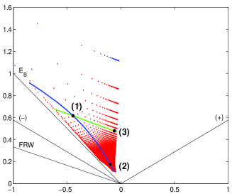
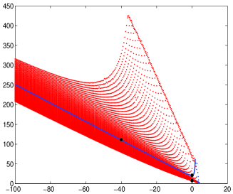
Figure 1: The figure on the left, from Ref. [6], shows the location in the $(\dot{\bar{\phi}},H)$ space of the fixed points for different choices of the parameters $c_{2}$ and $c_{4},$ and the corresponding ratio $\xi\equiv\dot{\bar{\phi}}/H$. The blue line shows the $c_{2}$-dependence of the fixed points for a constant $c_{4}=1$, while the green line shows the $c_{4}$-dependence for a constant $c_{2}=0$. The point labeled by (1) corresponds to $c_{2}=0,\,c_{4}=1$, with $\xi_{(1)}\simeq-0.72$. The point labeled by (2) corresponds to $c_{2}=-40,\,c_{4}=1$, with $\xi_{(2)}\simeq-0.56$. The point labeled by (3) corresponds to $c_{2}=0,\,c_{4}=15$, with $\xi_{(3)}\simeq-0.13$. On the right, we show the tree-level $\alpha^{\prime}$ asymptotic shift $c$ given by Eq. (35) as a function of the parameter $c_{2}$ and of the fixed point distribution. The blue line shows the evolution of the shift for a constant $c_{4}=1$.

4.2 Effective frequency shift

To describe the evolution of the high frequency modes, which are expected to leave the Hubble radius during the high curvature regime, we must use the perturbation equation Eq. (26), including those corrections required to regularise the background evolution. As mentioned in Section $3.2$, the incorporation of the higher-order corrections in the perturbation equation implies a time-dependence of the effective wavenumber $k$. Indeed, Eq. (26) can be conveniently rewritten

$$\psi_{k}^{\prime\prime}+\left\{k^{2}[1+c(\eta)]-V(\eta)\right\}\psi_{k}=0,$$ (34)

where we have introduced the effective shift in the comoving frequency $c\equiv(y^{2}-z^{2})/z^{2}$ which, at next-to-leading order in the string tension expansion, reads

$$c=\frac{2\alpha^{\prime}\left\{(4-c_{2}){\phi^{\prime}}^{2}-4(\phi^{\prime\prime}-2\frac{a^{\prime}\phi^{\prime}}{a})\right\}}{8a^{2}-\alpha^{\prime}\phi^{\prime}\left\{8\frac{a^{\prime}}{a}-c_{2}\phi^{\prime}\right\}}.$$ (35)

In the weak coupling regime, and for small curvature $(\alpha^{\prime}\rightarrow 0)$, the shift in the frequency is zero, hence no modification to the DDI cubic branch of the relic gravitational spectrum is expected. However, this frequency shift will be no longer negligible when $H\sim{\cal O}(\alpha^{\prime})$. In general, we find that $c(\eta)$ tends to grow, although a short decrease (which still satisfies $c(\eta)>-1$) may happen at the onset of the string phase. We also observe that the modification arising in the asymptotic regime, where the curvature is saturated by a linearly growing dilaton, corresponds to a constant shift of the comoving frequency, as first suggested in [33]. In that case, by setting $\dot{\phi}={\phi^{\prime}}/a\equiv\tilde{\phi}$ and $H=a^{\prime}/a^{2}\equiv\tilde{H}$, we can rewrite the asymptotic version of Eq. (35) as

$$c=\frac{2\alpha^{\prime}\tilde{\phi}\left\{(4-c_{2})\tilde{\phi}+4\tilde{H}\right\}}{8+\alpha^{\prime}\tilde{\phi}\left\{c_{2}\tilde{\phi}-8\tilde{H}\right\}}.$$ (36)

During such an intermediate string phase the external potential reduces to its tree-level version, namely $V(\eta)=\xi^{\prime\prime}/\xi,\quad\xi=ae^{-\phi/2}$, and the enhancement in frequency associated to Eq. (35) is the same for all modes, since the shift $c$ does not depend on the wavenumber $k$.

In Fig. 1 we have represented the effective shift as a function of the parameter $c_{2}$, highlighting the $c_{2}$-dependence by drawing the curve for $c_{4}=1$. Although the asymptotic shift cannot be expressed as a function of an unique variable, it is however possible to extract its minimal value for the type of $\alpha^{\prime}$ correction we are considering. The numerical simulations suggest that the lowest shifts correspond to fixed points located near the branch change line, $\dot{\bar{\phi}}\equiv\dot{\phi}-3H=0$. The bound $c_{2}=38/9$ attached to the sign change of $\dot{\overline{\phi}}$ implies that, in the limit of large values of $\tilde{\phi}$, the effective asymptotic shift is always positive, and is given by $c\geq 10/7$.

Does the frequency shift have any implication on the spectral distribution? In principle the answer is yes, since higher frequency modes tend to leave the Hubble radius at larger values of $H$ in the pre-Big Bang scenario. As a consequence, a given comoving mode will spend less time under the potential barrier, resulting in a smaller amplification of the frequency attached to this mode. Although it is difficult to quantify such an effect, we believe the higher-curvature corrections amount to an overall rescaling, by a numerical factor of order unity, of the total energy density of the background, as already discussed in [33].

Finally, the form of the effective shift Eq. (35) suggests that a background undergoing a non-singular evolution in the vicinity of $8-8\dot{\phi}H+c_{2}\dot{\phi}^{2}=0$ will automatically imply a rapid growth (if not a divergence) of the amplitude of the tensor fluctuations. Hence, we can understood the denominator of Eq. (35) as a source of quantum gravitational instability, of the type already discussed in [48, 49].

4.3 Full corrections and non-singular evolution

In recent studies of the graceful exit problem, in the context of the pre-Big Bang scenario, the regularisation of the background curvature and the transition to the post-Big Bang regime, are obtained by including quantum loop corrections, according to Eq. (8).

In this context, we may note that the tree-level $\alpha^{\prime}$ shift Eq. (35) provides an interesting constraint on the choice of parameters we can use in order to implement such a graceful exit, since in general the divergence curve for the high curvature shift is very close to the condition for the fixed point in the $(\dot{\bar{\phi}},H)$ plane. In [6], it has been shown that for a constant $c_{4}$ the fixed point value of the Hubble parameter tends to be reduced when $c_{2}$ is decreasing. Simultaneously the location of the singularity curve also decreases in the $(\dot{\bar{\phi}},H)$ plane, so that the range of coefficients leading to a non-singular evolution of the background, and avoiding the instability of quantum fluctuations, is strongly restricted to values very close to the simplest case of $\alpha^{\prime}$ correction, ${\cal L}_{\alpha^{\prime}}\sim\{R^{2}_{GB}-(\nabla\phi)^{4}\}$ (as also discussed in [32]). This is an unexpected, although fortunate constraint on the loop corrections, which allows restricting the range of values for the parameters $d_{i}$ and $e_{i}$.

In our attempt to characterise the power spectrum of metric perturbations generated in such a class of non-singular models, we will thus consider the perturbation equation Eq. (34) with a full shift determined by

$$c=\frac{2\alpha^{\prime}\left\{{\phi^{\prime}}^{2}\left[4-c_{2}-Ad_{2}e^{\phi}-(4e_{1}+e_{2})Be^{2\phi}\right]-4\left(\phi^{\prime\prime}-2\frac{a^{\prime}\phi^{\prime}}{a}\right)\left[1+4Be_{1}e^{2\phi}\right]\right\}}{8a^{2}-\alpha^{\prime}\phi^{\prime}\left\{8\frac{a^{\prime}}{a}\left[1+Be_{1}e^{2\phi}\right]-\phi^{\prime}\left[c_{2}+Ad_{2}e^{\phi}+Be_{2}e^{2\phi}\right]\right\}}.$$ (37)

Here the coefficients of the high curvature, one- and two loop corrections are respectively $c_{i},\;d_{i}$ and $e_{i}$, with $c_{1}=-1$ from the constraint Eq. (7).

As already stressed, this frequency shift reduces to a constant in the asymptotic stage of the string phase. The loop corrections re-establish the time-dependence during the graceful exit, but its contribution soon becomes negligible at the end of the phase of accelerated evolution. Indeed, Eq. (23) – Eq. (24) rapidly reduce to their tree-level expressions $y\simeq z\simeq ae^{-\phi/2}$, hence we expect $k_{eff}\rightarrow k$ before we enter the radiation-dominated epoch, where the frequency shift vanishes identically.

4.4 Observable implications

We are interested in the generic features of the primordial gravitational waves, generated by quantum fluctuations of the background metric during the pre-Big Bang phase, which could be detected by both ground-based detectors such as LIGO [50] and VIRGO [51], and space-based experiments such as LISA [52] (see also [53] for a recent review and references therein). For such a purpose, we use the dimensionless spectral energy density of perturbations, $\Omega_{gw}(\omega)$, to describe the background of gravitational radiation. In critical units, the energy density is defined by

$$\Omega_{gw}(\omega,t)\equiv\frac{1}{\rho_{c}}\frac{d\rho_{gw}}{d\ln\omega},$$ (38)

where $d\rho_{gw}$ is the present energy density in the stochastic gravitational waves per logarithmic interval of frequency, $\omega(t)=k/a(t)$ is the physical (angular) frequency of the wave, and $\rho_{c}(t)=3M_{p}^{2}H^{2}(t)/8\pi$ is the critical energy density required to close the universe.

Following the standard procedure for the computation of the energy spectrum [45], we must determine the expectation number of gravitons per cell of the phase space, $n(\vec{x},\vec{k})=n_{f}$, which only depends on the frequency for an isotropic and stochastic background. Neglecting $\alpha^{\prime}$ and loop corrections, both in the background and perturbation equations, the lowest order result Eq. (33) leads to [7]

$$\Omega_{gw}(\omega,t)\simeq\frac{8}{3\pi}\frac{\omega_{1}^{4}}{M_{p}^{2}H^{2}}\left(\frac{\omega}{\omega_{1}}\right)^{3},~{}\hskip 28.45274pt\omega<\omega_{1}$$ (39)

where $\omega_{1}=k_{1}/a=H_{1}a_{1}/a$ is the maximal amplified proper frequency, associated with the value $H_{1}$ of the Hubble expansion parameter at the end of the string phase.

Including higher-order corrections, the relation between the ultraviolet cutoff of the spectrum and the time of horizon crossing is in general more complicated, and a precise definition of the maximal amplified frequency is out of reach without a complete analytic solution for the background dynamics. However, a reliable estimate of the slope of the intermediate string branch of the spectrum can be obtained by using the leading features of the string phase.

First, we shall neglect (during the string phase) the effective frequency shift in the perturbation equation, whose role is simply expected to induce an overall rescaling of the amplitude [33], as already pointed out in Section 4.2. Second, we will assume that the duration of the “exit phase” is small compared to the intermediate string phase, and that no dramatic physics take place during the transition to the standard radiation-dominated epoch (indeed, in some cases where the exit is catalysed by the loop corrections, the process is almost instantaneous). This is a big assumption, of course, which could possibly underestimate “pre-heating” and “re-heating” effects. However, the accuracy of these assumptions can be confirmed with numerical simulations.

In summary, we suppose that the evolution of the background consists mainly of three phases: an initial, low energy dilaton-driven branch, the intermediate string phase with a constant Hubble parameter ($\tilde{H}$) and a linearly growing dilaton ($\dot{\phi}=\tilde{\phi}=$ const), and the final radiation phase with decreasing Hubble parameter and frozen dilaton. It follows from our assumptions that the spectral graviton distribution can be correctly estimated through the low-energy perturbation equation, even for the high frequency branch of the spectrum.

In that case, it is already well known [17] that the slope of the high-frequency modes, crossing the horizon in the high curvature, stringy regime, and re-entering in the radiation era, is fully determined by the fixed point values $\tilde{\phi},\tilde{H}$. Indeed, during such a string phase, the scale factor undergoes the usual de Sitter exponential expansion, while the logarithmic evolution of the dilaton, in conformal time, is weighted by the ratio $\tilde{\phi}/\tilde{H}$, i.e. $\phi(\eta)\sim-(\tilde{\phi}/\tilde{H})\log(-\eta)+$ const [54]. By introducing the convenient shifted variable $\tilde{\overline{\phi}}\equiv\tilde{\phi}-3\tilde{H}$, and referring the spectrum to a fixed point allowing a subsequent (loop catalysed) exit, i.e. $\tilde{\overline{\phi}}<0$, one easily finds [17]

$$\Omega_{gw}\sim\left(\frac{\omega}{\omega_{1}}\right)^{3-\left|\tilde{\bar{\phi}}/\tilde{H}\right|},~{}\hskip 28.45274pt\omega_{s}\ll\omega\ll\omega_{1}$$ (40)

where $\omega_{s}$ is the limit frequency marking the transition to the high curvature regime.

In our model of the background evolution, on the other hand, the allowed fixed points $\tilde{\phi},\tilde{H}$ are located in the ($\dot{\overline{\phi}},H$) plane between the “Branch change line”, $\dot{\overline{\phi}}<0$, and the “Einstein Bounce”, $\dot{\overline{\phi}}<-H$, see Fig. 1 and [6]. It follows that, in the context of our approximations, the spectrum of tensor fluctuations, at high frequency, has a slope constrained by

$$\textrm{(Einstein Bounce)}\quad 2<3-\left|\tilde{\bar{\phi}}/\tilde{H}\right|<3\quad\textrm{(Branch change)}.$$ (41)

In order to check this important analytical result, we analysed numerical solutions for different choices of coefficients of the tree-level $\alpha^{\prime}$ corrections.

4.5 Numerical results

The spectral distribution of relic gravitational waves can be obtained by numerical integration of the perturbation equation Eq. (26), in the background Eq. (2–5). The initial conditions are chosen in the low curvature and weakly coupled regime and are thus based on the tree-level solutions, which provide an adequate description of this phase. We then evolve the system until a given mode re-enters the Hubble radius, in the late time FRW radiation-dominated epoch, where we extract the Bogoliubov coefficients by comparing the result of the simulation and the free-oscillating solution Eq. (32).

To highlight the impact of the time-dependence of the frequency shift, we first present the spectral distribution in a case where we do not consider the $\alpha^{\prime}$ and loop corrections in the perturbation equation Eq. (26). Fig. 2 illustrates the results of such a simulation,for the particular model of background corresponding to $c_{1}=d_{1}=e_{1}=-1$, $c_{4}=d_{4}=e_{4}=1$ (all the other $c_{i},d_{i},e_{i}=0$), $A=1$, $B=-2\times 10^{-3}$ and $\Gamma_{\phi}=5.63\times 10^{-4}$. We show, in particular, the non-singular evolution of $H$ and $\dot{\phi}$, and the evolution of the quantity $aH$, which enables us to determine if a given mode leaves the Hubble radius during the DDI phase or during the intermediate string phase. Finally, we present the graviton distribution for such a background, computed from Eq. (26), in units $k/k_{max}$, where $k_{max}={\rm Max}(aH)$ is a maximal amplified frequency.

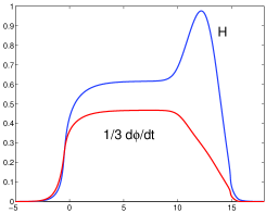
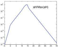
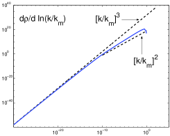
Figure 2: The choice of coefficients for the tree-level $\alpha^{\prime}$ corrections is $c_{1}=-1,\,c_{2}=c_{3}=0$ and $c_{4}=1$ (and the same for $d_{i}$ and $e_{i}$), corresponding to the case $(1)$ in Fig. 1. The left figure shows a non-singular evolution for the Hubble parameter $H=\dot{a}/a$ and for $\dot{\phi}/3$, as a function of the number of e-folds, $N=\ln a$. The middle figure shows the evolution of $aH/{\rm Max}(aH)$ as function of $N$. The low-energy, dilaton-driven phase takes place approximatively for $-\infty<N\leq-3$. After a short transition, this initial period is followed by a string phase with nearly constant Hubble parameter and linearly growing dilaton, for $2\leq N\leq 9$. After a successful exit triggered by loop corrections, the background evolution enters the FRW radiation-dominated phase at $N\simeq 16$. Comoving modes leaving the Hubble radius during the string phase ($10^{-6}\leq k/{\rm Max}(aH)\leq 10^{-2}$) are characterised by a slope smaller than $3$ in the spectral distribution, as illustrated in the right figure which shows $d\rho_{k}/d\ln(k)$ in units of $k/k_{max}$. The upper dashed line corresponds to the cubic slope typical of the low frequency part of the spectrum, emerging from the dilaton-driven epoch.

The effects of the higher-order corrections are expected to arise when the curvature scale becomes large in string units. As a consequence, the low frequency branch of the spectrum is unaffected by such corrections, and remains characterised by a cubic slope. However, modes leaving the Hubble radius during the intermediate string phase are strongly affected by the background dynamics. The resulting slope of the spectrum is found to be reduced, but remains confined between $2$ and $3$, as expected from Eq. (41).

Does the inclusion of the time-dependence of the comoving wavenumber lead to any modification? We stress that when such a shift in the frequency is considered, we have $k\sqrt{1+c}=aH$ at horizon crossing. As a consequence, the shortest scale to leave the Hubble radius is given by $k_{max}={\rm Max}\left(aH/\sqrt{1+c}\right)$, instead of ${\rm Max}(aH)$. This is illustrated in Fig. 3, where we compare the results of the numerical integration with and without corrections in the perturbation equation, for identical non-singular background evolutions (the same model of Fig. 2). No modification appears during the low energy epoch, where the frequency shift is negligible. However, higher-order corrections in the perturbation equation, which result in the time-dependent shift, lead to a reduction of the maximal amplified frequency and of the time spent on super-horizon scales.

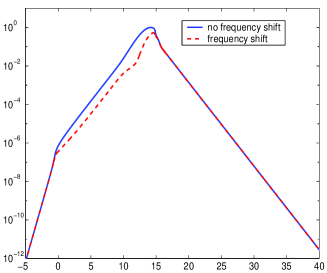
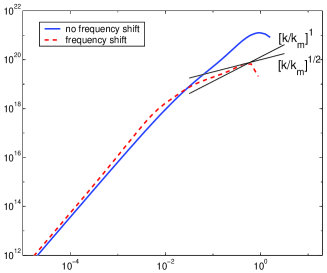
Figure 3: Using the same choice of coefficients as in Fig. 2, we compare the evolution of $aH/{\rm Max}(aH)$ (solid curve) and $aH/{\rm Max}\left(aH/\sqrt{1+c}\right)$ (dashed curve) as a function of $N$. When higher-order corrections are included in the perturbation equation, the high frequency cutoff and the duration of the super-horizon epoch are found to be reduced. The right hand figure is a magnified image of the end point of the string branch of the spectral distribution, which highlights the impact due to a non-trivial frequency shift: the significant new feature is the reduction of the high frequency peak and a further reduction of the slope, which may also become smaller than two, for comoving modes leaving the Hubble radius during the “exit phase”.

The impact of the time-dependence of the comoving wavenumber $k$ is non-trivial for very high-frequency modes, leaving the Hubble radius during the graceful exit to the FRW-radiation dominated epoch. In that case, the result Eq.(40) no longer applies, and the slope can be smaller than two, as shown in Fig. 3. However, the impact remains negligible for modes well inside the string branch of the spectrum i.e. for modes crossing the horizon during the asymptotic, fixed point regime. In that case, our analytical approximations for the slope of the spectrum are confirmed by the numerical simulations. In Table 1, we present the predicted and measured slopes well inside the string phase, for the three different choices of coefficients illustrated in Fig. 1. The agreement is striking.

	Coefficients at ${\cal O}(\alpha^{\prime})$		Predicted slope	Measured slope
	$c_{2}$	$c_{4}$	$3-\left|\tilde{\bar{\phi}}/\tilde{H}\right|$	(numerical)
Case $(1)$	$0$	$1$	$2.44$	$2.45$
Case $(2)$	$-40$	$1$	$2.28$	$2.3$
Case $(3)$	$0$	$15$	$2.87$	$2.85$

Table 1: Choices of coefficients for the tree-level $\alpha^{\prime}$ corrections with $c_{1}=-1$ and the remaining coefficient satisfying $c_{3}=-(c_{1}+c_{4}+c_{2}/2)$, according to Eq. (7). We have compared the predicted slope determined by the fixed point, according to Eq. (40), with the measured slope well inside the string branch of the spectrum, obtained by numerical integration of Eq. (26), including all corrections.

It is well known [44] that the spectrum of relic gravitons, in the context of the pre-Big Bang scenario, easily evades constraints arising from both the CMB anisotropy at COBE scale [55] and pulsar timing data [56], because of its rapid growth at low frequency. Hence, the peak amplitude of the spectrum is only constrained by the primordial nucleosynthesis bound [57], as well as by primordial black hole production [58].

The relic graviton background is in general compatible with these constraints if it is normalised so as to match the string scale at the high-frequency end point of the spectrum. In that case one finds [21] that the high frequency peak is typically of order $\Omega_{gw}(\omega)\simeq 10^{-6}$, for a maximal amplified frequency $\omega\simeq 10^{11}[{\rm Hz}]$. Saturating this high-frequency end point, and using the prediction Eq. (41) for the slope of the string branch of the spectrum, the energy density of relic gravitons from a pre-Big Bang phase could be at most of ${\cal O}(10^{-15})$ at $\omega\simeq 10^{2}[{\rm Hz}]$, regardless of the duration of the string phase with constant Hubble parameter, i.e. far below the sensitivity of the second (planned) generation of interferometric gravity wave detectors [53]. It seems thus difficult to detect the relic gravitons from a high curvature string phase, associated to a fixed point of the truncated effective action – at least within the model of background considered in this paper – unless the exit phase is able to affect a sufficiently wide band of the high frequency spectrum.

Finally, the numerical integration of Eq. (26) enables us to follow carefully the time evolution of modes, from the DDI epoch up to the FRW-radiation dominated era. We have explicitly checked that the amplitude of tensor perturbations is rapidly frozen in on super-horizon scale, regardless of the particular higher-order dynamics of the background during the string phase and the exit epoch.

5 Conclusion

In this paper we have discussed the evolution of tensor perturbations in a class of non-singular cosmological models based on the gravi-dilaton string effective action, expanded up to first order in $\alpha^{\prime}$, and including one-loop and two-loop corrections in the string coupling parameter.

The coefficients of the loop expansion have been chosen in such a way as to avoid the curvature singularities in the background, and the quantum instability of metric fluctuations. In addition, we have included an appropriate radiation backreaction to stabilise the dilaton in the final, post-Big Bang regime. We have been able to obtain, in this way, a class of regular cosmological solutions in which the initial Universe, emerging from the string perturbative vacuum, is first trapped in a fixed point of high, constant curvature, and then spontaneously undergoes a smooth transition to the standard FRW regime. The fixed point is determined by the $\alpha^{\prime}$ corrections, while the unstability and the decay of the high curvature regime is triggered by the quantum loop corrections.

We have determined, in this class of backgrounds, the linearised equation governing the evolution of tensor metric fluctuations, taking into account all the $\alpha^{\prime}$ and loop corrections contributing to the background regularisation. We have discussed, on this ground, the amplification of tensor perturbations normalised to the quantum fluctuations of the vacuum, and we have estimated their final spectral energy distribution through analytical and numerical methods.

Our results confirm previous expectations, that the low frequency modes, crossing the horizon in the low-curvature regime, are unaffected by higher-order corrections. Also, we have explicitly checked (through numerical simulations) that the so-called “string branch” of the spectrum, associated with the asymptotic, fixed point regime, can be reliably estimated by means of the low-energy perturbation equation, that its slope is determined by the asymptotic constant values of $H$ and $\dot{\phi}$, and that it is flatter than at low frequency.

However, when the background regularisation crosses a fixed point, and when the fixed point is determined by the $\alpha^{\prime}$ expansion truncated to first order (like in the class of models of this paper), it turns out that the slope of the string branch is at least quadratic, and thus probably too steep to be compatible with future observations by planned advanced detectors. In the transition regime dominated by the quantum loops, on the other hand, the influence of the higher-order corrections on tensor perturbations is more dramatic, and the corresponding slope may be much flatter than the one of the preceding string phase.

In summary, the results of this paper agree with the general expectation that the shape of the spectrum of the relic graviton background, obtained in the context of the pre-Big Bang scenario, is strongly model-dependent. However, it turns out that the formulation of a complete and consistent regular scenario, associated to a “visible” graviton spectrum, may be more difficult than previously expected – at least within a truncated perturbative approach, like the one adopted in this paper.

References

- [1] G. Veneziano. Scale factor duality for classical and quantum strings. Phys. Lett., B265:287–294, 1991, CERN-TH.6077/91.
- [2] M. Gasperini and G. Veneziano. Pre-Big Bang in string cosmology. Astropart. Phys., 1:317–339, 1993, hep-th/9211021. An updated collection of papers and references on the pre-Big Bang scenario is available at the URL, http://www.to.infn.it/gasperin/.
- [3] R. Brustein and R. Madden. A model of graceful exit in string cosmology. Phys. Rev., D57:712–724, 1998, hep-th/9708046.
- [4] S. Foffa, M. Maggiore and R. Sturani. Loop corrections and graceful exit in string cosmology. Nucl. Phys., B552:395, 1999, hep-th/9903008.
- [5] R. Brustein and R. Madden. Classical corrections in string cosmology. JHEP, 07:006, 1999, hep-th/9901044.
- [6] C. Cartier, E.J. Copeland and R. Madden. The graceful exit in string cosmology. JHEP, 01:035, 2000, hep-th/9910169.
- [7] M. Gasperini and G. Veneziano. Dilaton production in string cosmology. Phys. Rev., D50:2519–2540, 1994, gr-qc/9403031.
- [8] L.P. Grishchuk. Amplification of gravitational waves in an isotropic universe. Sov. Phys. JETP, 40:409–415, 1975.
- [9] A.A. Starobinsky. Spectrum of relict gravitational radiation and the early state of the universe. JETP Lett., 30:682–685, 1979.
- [10] L.P. Grishchuk and M. Solokhin. Spectra of relic gravitons and the early history of the Hubble parameter. Phys. Rev., D43:2566–2571, 1991.
- [11] J. Garriga and E. Verdaguer. Particle creation due to cosmological contraction of extra dimensions. Phys. Rev., D39:1072, 1989.
- [12] M. Demianski. Dynamics of multidimensional Kaluza-Klein cosmological models. 1990. In *Capri 1990, Proceedings, General relativity and gravitational physics* 19-41.
- [13] M. Gasperini and M. Giovannini. Gravity waves from primordial dimensional reduction. Class. Quant. Grav., 9:L137, 1992.
- [14] M. Gasperini and M. Giovannini. Dilaton contributions to the cosmic gravitational wave background. Phys. Rev., D47:1519–1528, 1993, gr-qc/9211021.
- [15] J.D. Barrow, J.P. Mimoso and M.R. de Garcia Maia. Amplification of gravitational waves in scalar - tensor theories of gravity. Phys. Rev., D48:3630–3640, 1993.
- [16] M. Gasperini and M. Giovannini. Constraints on inflation at the Planck scale from the relic graviton spectrum. Phys. Lett., B282:36–43, 1992.
- [17] R. Brustein, M. Gasperini, M. Giovannini and G. Veneziano. Relic gravitational waves from string cosmology. Phys. Lett., B361:45–51, 1995, hep-th/9507017.
- [18] R.B. Abbott, B. Bednarz and S.D. Ellis. Cosmological perturbations in Kaluza-Klein models: Appendix. Phys. Rev., D33:2147, 1986.
- [19] M. Gasperini and G. Veneziano. Inflation, deflation, and frame independence in string cosmology. Mod. Phys. Lett., A8:3701–3714, 1993, hep-th/9309023.
- [20] R. Brustein, M. Gasperini, M. Giovannini, V.F. Mukhanov and G. Veneziano. Metric perturbations in dilaton driven inflation. Phys. Rev., D51:6744–6756, 1995, hep-th/9501066.
- [21] R. Brustein, M. Gasperini and G. Veneziano. Peak and endpoint of the relic graviton background in string cosmology. Phys. Rev., D55:3882–3885, 1997, hep-th/9604084.
- [22] D. Polarski and A.A. Starobinsky. Semiclassicality and decoherence of cosmological perturbations. Class. Quant. Grav., 13:377–392, 1996, gr-qc/9504030.
- [23] K.S. Thorne. Gravitational radiation: A new window onto the universe. 1997, gr-qc/9704042.
- [24] B. Allen and J.D. Romano. Detecting a stochastic background of gravitational radiation: Signal processing strategies and sensitivities. Phys. Rev., D59:102001, 1999, gr-qc/9710117.
- [25] M. Gasperini, J. Maharana and G. Veneziano. From trivial to nontrivial conformal string backgrounds via 0(d,d) transformations. Phys. Lett., B272:277–284, 1991.
- [26] M. Gasperini. Looking back in time beyond the Big Bang. Mod. Phys. Lett., A14:1059, 1999, gr-qc/9905062.
- [27] M. Gasperini, J. Maharana and G. Veneziano. Boosting away singularities from conformal string backgrounds. Phys. Lett., B296:51–57, 1992, hep-th/9209052.
- [28] M. Giovannini. Regular cosmological examples of tree-level dilaton-driven models. Phys. Rev., D57:7223–7234, 1998, hep-th/9712122.
- [29] R. Brustein and G. Veneziano. The graceful exit problem in string cosmology. Phys. Lett., B329:429–434, 1994, hep-th/9403060.
- [30] I. Antoniadis, J. Rizos and K. Tamvakis. Singularity - free cosmological solutions of the superstring effective action. Nucl. Phys., B415:497–514, 1994, hep-th/9305025.
- [31] S.J. Rey. Back reaction and graceful exit in string inflationary cosmology. Phys. Rev. Lett., 77:1929–1932, 1996, hep-th/9605176.
- [32] M. Gasperini, M. Maggiore and G. Veneziano. Towards a nonsingular pre-Big Bang cosmology. Nucl. Phys., B494:315–330, 1997, hep-th/9611039.
- [33] M. Gasperini. Tensor perturbations in high curvature string backgrounds. Phys. Rev., D56:4815–4823, 1997, gr-qc/9704045.
- [34] A. Feinstein, K.E. Kunze and M.A. Vazquez-Mozo. Initial conditions and the structure of the singularity in pre-Big Bang cosmology. Class. Quant. Grav., 17:3599–3616, 2000, hep-th/0002070.
- [35] A. Buonanno, T. Damour and G. Veneziano. Pre-Big Bang bubbles from the gravitational instability of generic string vacua. Nucl. Phys., B543:275, 1999, hep-th/9806230.
- [36] R.R. Metsaev and A.A. Tseytlin. Order (two-loop) equivalence of the string equations of motion and the sigma model weyl invariance conditions: dependence on the dilaton and the antisymmetric tensor. Nucl. Phys., B293:385, 1987.
- [37] N. Kaloper and K.A. Olive. Dilatons in string cosmology. Astropart. Phys., 1:185–194, 1993.
- [38] A.A. Starobinsky. Evolution of small excitation of isotropic cosmological models with one loop quantum gravitation corrections. Zh. Eksp. Teor. Fiz., 34:460, 1981. (In russian).
- [39] V.F. Mukhanov, L.A. Kofman and D.Y. Pogosyan. Cosmological perturbations in the inflationary universe. Phys. Lett., B193:427–432, 1987.
- [40] L. Amendola, M. Litterio and F. Occhionero. Very large angular scales and very high-energy physics. Phys. Lett., B231:43–48, 1989.
- [41] H. Noh and J.C. Hwang. Cosmological gravitational wave in a gravity with quadratic order curvature couplings. Phys. Rev., D55:5222–5225, 1997, gr-qc/9610059.
- [42] A. Buonanno, M. Maggiore and C. Ungarelli. Spectrum of relic gravitational waves in string cosmology. Phys. Rev., D55:3330–3336, 1997, gr-qc/9605072.
- [43] A. Buonanno, K.A. Meissner, C. Ungarelli and G. Veneziano. Quantum inhomogeneities in string cosmology. JHEP, 01:004, 1998, hep-th/9710188.
- [44] M. Gasperini. Elementary introduction to pre-Big Bang cosmology and to the relic graviton background. 1999, hep-th/9907067. Proc. of the Second SIGRAV School on Gravitational Waves (Centre A. Volta, Como, April 1999), eds. I. Ciufolini et al. (IOP Publishing, Bristol, 2001), p. 280.
- [45] V.F. Mukhanov, H.A. Feldman and R.H. Brandenberger. Theory of cosmological perturbations. Phys. Rept., 215:203–333, 1992.
- [46] R. Brustein, M. Gasperini and G. Veneziano. Duality in cosmological perturbation theory. Phys. Lett., B431:277–285, 1998, hep-th/9803018.
- [47] R. Brustein and R. Madden. Graceful exit and energy conditions in string cosmology. Phys. Lett., B410:110, 1997, hep-th/9702043.
- [48] S. Kawai, M. Sakagami and J. Soda. Perturbative analysis of non-singular cosmological model. 1997, gr-qc/9901065.
- [49] S. Kawai and J. Soda. Evolution of fluctuations during graceful exit in string cosmology. Phys. Lett., B460:41, 1999, gr-qc/9903017.
- [50] B. Allen and R. Brustein. Detecting relic gravitational radiation from string cosmology with LIGO. Phys. Rev., D55:3260–3264, 1997, gr-qc/9609013.
- [51] D. Babusci and M. Giovannini. Sensitivity of a VIRGO pair to stochastic gravitational waves backgrounds. Class. Quant. Grav., 17:2621–2633, 2000, gr-qc/0008041.
- [52] C. Ungarelli and A. Vecchio. Are pre-big-bang models falsifiable by gravitational wave experiments? 1999, gr-qc/9911104.
- [53] M. Maggiore. Gravitational wave experiments and early universe cosmology. Phys. Rept., 331:283, 2000, gr-qc/9909001.
- [54] M. Gasperini, M. Giovannini and G. Veneziano. Electromagnetic origin of the cosmic microwave backgrounds anisotropy in string cosmology. Phys. Rev., D52:6651–6655, 1995, astro-ph/9505041.
- [55] C.L. Bennett et al. Astrophys. J., 430:423, 1994.
- [56] V.M. Kaspi, J. Taylor and M. Ryba. Evolution of fluctuations during graceful exit in string cosmology. Astrophys. J., 428:1519, 1994.
- [57] T.P. Walker, G. Steigman, D.N. Schramm, K.A. Olive and H.S. Kang. Primordial nucleosynthesis redux. Astrophys. J., 376:51–69, 1991.
- [58] E.J. Copeland, A.R. Liddle, J.E Lidsey and D. Wands. Black holes and gravitational waves in string cosmology. Phys. Rev., D58:063508, 1998, gr-qc/9803070.