Collision of spinning black holes in the close limit

Abstract

In this paper we consider the collision of spinning holes using first order perturbation theory of black holes (Teukolsky formalism). With these results (along with ones, published in the past) one can predict the properties of the gravitational waves radiated from the late stage inspiral of two spinning, equal mass black holes. Also we note that the energy radiated by the head-on collision of two spinning holes with spins (that are equal and opposite) aligned along the common axis is more than the case in which the spins are perpendicular to the axis of the collision.

I Introduction

There is considerable current interest in studying the collision of two black holes, since these events could be primary sources of gravitational waves for interferometric gravitational wave detectors currently under construction. The mathematics describing such events consists of the nonlinear partial differential equations of general relativity, Einstein’s theory of gravitation. These equations are very difficult to solve especially in the case of two merging holes, or of the highly distorted final hole that is formed by the merger. Limited (in resolution and evolution time) full numerical simulations of grazing collisons of black holes are being done now [1], but long term stable evolutions are still distant in the future. It is therefore of interest to have at hand approximate results which in certain regimes could be used to test and possibly even complement the full numerical evolutions. Among such approximation methods is the “close-limit” approximation in which spacetime of a black hole collision is represented as a single distorted black hole and evolutions are done with simple linear perturbative equations. In the past, this method has been applied to the case of a head-on collision of two boosted holes [2] and the case of slow inspiral [3] with considerable success. In both these cases, the black holes considered had no spin. In this work, we will consider the collision of spinning holes.

Since we are attempting a linear, first order perturbative calculation, it is sufficient to study the coalescence of two spinning holes with zero initial linear momentum. This is because, to obtain the results for the inspiral of spinning holes, one can simply do a linear superposition of these results with those from our past work [3]. However, the first order perturbative treatment imposes several restrictions on the physical scenarios we can treat. In addition to the close-slow limitations, we can only easily analyze cases in which the spins of the two black holes are equal and opposite. This happens because, to lowest order, the (perturbative) extrinsic curvature of a black hole with spin $S$ and a conformal distance $L$ from the origin is of order $SL$. Superposing another hole with parallel and equal spin and at $-L$ will yield a situation with zero perturbation in extrinsic curvature, which is not a case of interest.

So in the following, we shall present two cases that are exhaustive. Case I, when the two spins are equal and opposite and aligned along the common axis of the two holes. Specifically, we place the two holes at $x=\pm L/2$ and have their spins parallel and anti-parallel to the x-axis. Case II, when the two spins are equal and opposite and perpendicular to the common axis of the two holes. Here, we place the two holes at $x=\pm L/2$ and have their spins parallel and anti-parallel to the y-axis. These cases have no net angular momentum. So we expect Zerilli and Teukolsky formalisms to agree exactly (Kerr parameter $a=0$). We, therefore report calculations and results from the Teukolsky formalism only. Part of this work, in the context of the Zerilli formalism can be found in this reference [4].

II Initial data

To evolve a spacetime in general relativity, one needs to provide initial data, a 3-geometry $g_{ab}$ and an extrinsic curvature $K_{ab}$, that solve Einstein’s equations on some starting hypersurface (i.e., at some starting time). These initial value equations have the form,

$$\nabla^{a}(K_{ab}-g_{ab}K) = 0$$ (1)

$${}^{3}R-K_{ab}K^{ab}+K^{2} = 0$$ (2)

where $g_{ab}$ is the spatial metric, $K_{ab}$ is the extrinsic curvature and ${}^{3}R$ is the scalar curvature of the three metric. If we propose a 3-metric that is conformally flat $g_{ab}=\phi^{4}\widehat{g}_{ab}$, with $\widehat{g}_{ab}$ a flat metric, and $\phi^{4}$ the conformal factor, and we use a decomposition of the extrinsic curvature $K_{ab}=\phi^{-2}\widehat{K}_{ab}$, and assume maximal slicing $K_{a}^{a}=0$, the constraints become,

$$\widehat{\nabla}^{a}\widehat{K}_{ab} = 0$$ (3)

$$\widehat{\nabla}^{2}\phi = -\frac{1}{8}\phi^{-7}\widehat{K}_{ab}\widehat{K}^{ab}\ ,$$ (4)

where $\widehat{\nabla}$ is a flat-space covariant derivative.

To solve the momentum constraint, we start with a solution that represents a single hole with spin $S$ [10],

$$\hat{K}^{\rm one}_{ab}={3\over r^{3}}\left[{\epsilon_{cad}}{S^{d}}{n^{c}}{n_{b}}+{\epsilon_{cbd}}{S^{d}}{n^{c}}{n_{a}}\right]\ .$$ (5)

In this expression for the conformally related extrinsic curvature at some point $x^{a}$, the quantity $n_{b}$ is a unit vector, in the “base” flat space with metric $\hat{g}_{ab}$, directed from a point representing the location of the hole to the point $x^{a}$. The symbol $r$ represents the distance, in the flat base space, from the point of the hole to $x^{a}$. It is straightforward to show that the solution of the Hamiltonian constraint corresponding to eq. (5) corresponds to a spacetime with ADM angular momentum $S^{a}$.

The next step is to modify this to represent holes centered at $x=\pm L/2$ in the conformally flat metric. Since the momentum constraint is linear, we can simply add two expressions of the above form,

$$\widehat{K}^{\rm two}_{ab}=\widehat{K}^{\rm one}_{ab}\left(x\rightarrow x-L/2,{S_{x}\,{\rm or}\,S_{y}}=S\right)+\widehat{K}^{\rm one}_{ab}\left(x\rightarrow x+L/2,{S_{x}\,{\rm or}\,S_{y}}=-S\right)\ .$$ (6)

We will choose in further expressions to use a polar coordinate system in the flat space determined by $\hat{g}_{ab}$ centered in the mid-point separating the two holes and label the polar coordinates as $(R,\theta,\phi)$. So $R$ will be the distance in the flat space from the midpoint between the holes.

To solve the Hamiltonian constraint 4, we introduce an approximation, (the slow approximation) which we will show is enough for our purposes. In fact, in this approximation the solution for the conformal factor turns out to be the familiar Misner [6] solution if one chooses the topology of the slice to have a single asymptotically flat region, or the Brill–Lindquist [8] solution if there are three asymptotically flat regions.

A The slow approximation

We assume that the black holes are initially close, and that the initial spins $S$ are small. We denote by $\vec{n}^{+}$ and $\vec{n}^{-}$ the normal vectors corresponding, respectively, to the one hole solutions at $x=+L/2$ and at $x=-L/2$, and we recall $R$ to be the distance to a field point, in the flat conformal space, from the point midway between the holes. For large $R$, the normal vectors $\vec{n}^{+}$ and $\vec{n}^{-}$ almost cancel. More specifically $\vec{n}^{+}=-\vec{n}^{-}+O(L/R)$. A consequence of this is that the total initial $\widehat{K}^{ab}$ is first order in $L/R$. It scales linearly with the spin $S$ as well. Thus the source term in the Hamiltonian constraint is quadratic in $S$. If we choose to find a solution to the conformal factor to first order in $S$ (which should give us a good approximation in the case of slowly spinning holes), we can ignore this quadratic source term. So now, the Hamiltonian constraint looks like the one for zero momentum, which is simply the Laplace equation. A well known solution to this, is the Misner solution [6]. This solution, is characterized by a parameter $\mu_{0}$ which describes the separation of the two throats. We can relate this parameter to the conformal distance $L$ in the following way [7],

$$L/M=\frac{\rm{\coth}\mu_{0}}{2\Sigma_{1}}\ \ \hskip 30.0pt\ \ \ \Sigma_{1}\equiv\sum_{n=1}\frac{1}{\sinh n\mu_{0}}\ .$$ (7)

We must now map the coordinates of the initial value solution to the coordinates for the Schwarzschild (Kerr with $a=0$) background. To do this, we interpret the $R$ as the isotropic radial coordinate of a Schwarzschild spacetime, and we relate it to the usual Schwarzschild radial coordinate $r$ by $R=(\sqrt{r}+\sqrt{r-2M})^{2}/4$. From this we arrive at the following expressions for the components of the metric and extrinsic curvature.

B Initial data for the Teukolsky function – Case I

Following the construction as outlined in the last section, we get the following expressions for the initial spatial metric and extrinsic curvature:

$${K}_{ab}={3SL\over Rr^{2}}\left[\begin{array}[]{ccc}0&\frac{-2\sin\theta\sin 2\varphi}{\sqrt{1-2M/r}}&\frac{-2\sin\theta\sin 2\theta\cos^{2}\varphi}{\sqrt{1-2M/r}}\\ \frac{-2\sin\theta\sin 2\varphi}{\sqrt{1-2M/r}}&r\cos\theta\sin 2\varphi&r\sin\theta(\cos^{2}\theta\cos^{2}\varphi-\sin^{2}\varphi)\\ \frac{-2\sin\theta\sin 2\theta\cos^{2}\varphi}{\sqrt{1-2M/r}}&r\sin\theta(\cos^{2}\theta\cos^{2}\varphi-\sin^{2}\varphi)&-r\sin^{2}\theta\cos\theta\sin 2\varphi\end{array}\right]\ .$$ (8)

The metric has a form, identical to the Misner solution [6]. Now, we use the methodology and expressions in [3], to find the initial data for the Teukolsky function, $\Psi={\rho}^{-4}\psi_{4}$, where ${\rho}={-1/{(r-ia\cos\theta)}}$.

For the azimuthal modes $m=\pm 2$ we get these expressions,

$$-{\Psi\over\sqrt{2\pi}}=-{3\over 4}i(\cos\theta\pm 1)^{2}LS\frac{(r-2M)(-1+2\sqrt{1-{2M\over r}})}{r(r(1+\sqrt{1-{2M\over r}})-M)}$$ (9)

$$-{\dot{\Psi}\over\sqrt{2\pi}}=-{3\over 4}i(\cos\theta\pm 1)^{2}LS\frac{(r-2M)(-3r+8M+3(r-7M)\sqrt{1-{2M\over r}})}{r^{3}(r(1+\sqrt{1-{2M\over r}})-M)}.$$ (10)

And for the azimuthal mode $m=0$ we get,

$$-{\Psi\over\sqrt{2\pi}}={3\over 2}i\sin^{2}\theta LS\frac{(r-2M)(-1+2\sqrt{1-{2M\over r}})}{r(r(1+\sqrt{1-{2M\over r}})-M)}$$ (11)

$$-{\dot{\Psi}\over\sqrt{2\pi}}={3\over 2}i\sin^{2}\theta LS\frac{(r-2M)(-3r+8M+3(r-7M)\sqrt{1-{2M\over r}})}{r^{3}(r(1+\sqrt{1-{2M\over r}})-M)}.$$ (12)

To all these expressions, we also need to add metric contributions. They have the same form as the ones in [3], therefore we will not list them here.

C Initial data for the Teukolsky function – Case II

Again, following the construction as outlined in the last section, and using the close-slow approximation, we arrive at the following expressions for the initial spatial metric and extrinsic curvature:

$${K}_{ab}={3SL\over Rr^{2}}\left[\begin{array}[]{ccc}\frac{2\cos\theta}{r-2M}&\frac{\sin\theta(4\cos^{2}\varphi-1)}{\sqrt{1-2M/r}}&\frac{-\sin 2\theta\sin\theta\sin 2\varphi}{\sqrt{1-2M/r}}\\ \frac{\sin\theta(4\cos^{2}\varphi-1)}{\sqrt{1-2M/r}}&-2r\cos\theta\cos^{2}\varphi&{r\over 2}\sin\theta(1+\cos^{2}\theta)\sin 2\varphi\\ \frac{-\sin 2\theta\sin\theta\sin 2\varphi}{\sqrt{1-2M/r}}&{r\over 2}\sin\theta(1+\cos^{2}\theta)\sin 2\varphi&-{r\over 2}\sin\theta\sin 2\theta\sin 2\varphi\end{array}\right]\ .$$ (13)

The metric again has a form, identical to the Misner solution [6]. Using the methodology and expressions we discussed in [3], the initial data for the Teukolsky function, is:

For the azimuthal modes $m=\pm 2$ we get,

$$-{\Psi\over\sqrt{2\pi}}=\mp{3\over 4}(\cos\theta\pm 1)^{2}LS\frac{(r-2M)(-1+2\sqrt{1-{2M\over r}})}{r(r(1+\sqrt{1-{2M\over r}})-M)}$$ (14)

$$-{\dot{\Psi}\over\sqrt{2\pi}}=\mp{3\over 4}(\cos\theta\pm 1)^{2}LS\frac{(r-2M)(-3r+8M+3(r-7M)\sqrt{1-{2M\over r}})}{r^{3}(r(1+\sqrt{1-{2M\over r}})-M)}.$$ (15)

And for the azimuthal mode, $m=0$ the initial data are identically zero. To all these expressions we need to add the metric contributions, that have a form identical to the ones in our past work [3].

III Evolution of the Data using the Teukolsky equation

Given the Cauchy data from the last section, the time evolution is obtained from the Teukolsky equation [9],

$$\Biggr{\{}\left[a^{2}\sin^{2}\theta-\frac{(r^{2}+a^{2})^{2}}{\Delta}\right]\partial_{tt}-\frac{4Mar}{\Delta}\partial_{t\varphi}+4\left[r+ia\cos\theta-\frac{M(r^{2}-a^{2})}{\Delta}\right]\partial_{t}$$ (16)

$$+\,\Delta^{2}\partial_{r}\left(\Delta^{-1}\partial_{r}\right)+\frac{1}{\sin\theta}\partial_{\theta}\left(\sin\theta\partial_{\theta}\right)+\left[\frac{1}{\sin^{2}\theta}-\frac{a^{2}}{\Delta}\right]\partial_{\varphi\varphi}$$ (17)

$$-\,4\left[\frac{a(r-M)}{\Delta}+\frac{i\cos\theta}{\sin^{2}\theta}\right]\partial_{\varphi}-\left(4\cot^{2}\theta+2\right)\Biggr{\}}\Psi=0,$$ (18)

where $M$ is the mass of the black hole, $a$ its angular momentum per unit mass (which is zero in our case), $\Sigma\equiv r^{2}+a^{2}\cos^{2}\theta$, and $\Delta\equiv r^{2}-2Mr+a^{2}$. Evolving the initial data we just calculated, with this equation will enable us to extract gravity wave waveforms that correspond to the late stage merger of spinning holes. We can also estimate the energy carried away by these gravitational waves. The radiated energy is given by [12],

$$\frac{dE}{dt}=\lim_{r\to\infty}\left\{\frac{1}{4\pi r^{6}}\int_{\Omega}d\Omega\left|\int_{-\infty}^{t}d\tilde{t}\ \Psi(\tilde{t},r,\theta,\varphi)\right|^{2}\right\},\quad d\Omega=\sin\theta\ d\vartheta\ d\varphi.$$ (19)

Note that the angular momentum radiated in the cases we consider is zero.

IV Results of the evolutions

In this section we show waveforms and plots for energy radiated from the collision of two spinning holes. Recall that the two holes have equal mass and equal and opposite spin, and we are considering two cases, Case I in which the spins are aligned along the common axis of the two holes, and Case II in which the two spins are perpendicular to the common axis of the two holes.

The waveforms that follow, are for a collision of two black holes that were initially separated by a conformal distance of $0.91$ and had an individual spin of $0.1$ in units of ADM mass.

In figure 1 we show the $m=2$ mode of the Teukolsky function for a Case I collision. We see the typical quasi-normal ringing, in both the real and imaginary parts of the function. In figure 2 we plot the $m=2$ mode of the Teukolsky function for a Case II collision. Note that the initial data is purely real for this case, hence the imaginary part of the waveform is identically zero. Quasi-normal ringing is self-evident here as well. This is the type of signal that gravity wave observatories like LIGO, will detect if they happen to witness a collision of the kind we are considering.

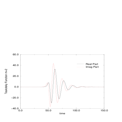
FIG. 1.: This figure depicts the $m=2$ mode of the Teukolsky function for a Case I collision. The solid line depicts the real part whereas the dotted one, the imaginary part. All quantities are in units of ADM mass.

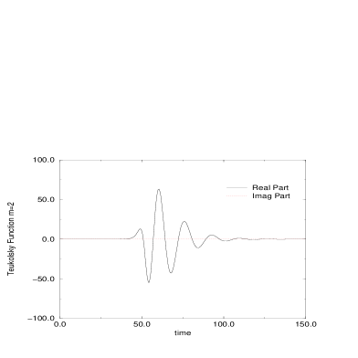
FIG. 2.: This figure shows the $m=2$ mode of the Teukolsky function for a Case II collision. The solid line depicts the real part whereas the dotted one, the imaginary part. All quantities are in units of ADM mass.

Let us turn now to the evaluation of the radiated energies for these two cases. Figure 3 shows the radiated energy as a function of the initial spin, for a fixed separation of the holes. The first noteworthy thing is that the two curves, corresponding to Case I and Case II are very close to each other throughout. This indicates that the geometry of the initial configuration does not matter much as far as energy loss is concerned. But, it should be observed that for any spin $S$, Case I radiates more than Case II. The next important observation (by looking at the trend of the curves for large spin) is that, even for high values of the initial spin of the two holes this type of collision radiates less than $1\%$ of its total mass. This means that inclusion of spin does not dramatically change our original estimate [3] [11] of a percent of the mass-energy being carried away by gravity waves in binary black hole inspiral.

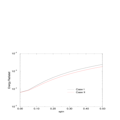
FIG. 3.: The radiated energy in a head-on collision of two spinning black holes as a function of the individual initial spin (that is equal and opposite for the two holes), for a fixed conformal separation of $0.91$. All quantities are in ADM mass units. Looking at the behavior of the curves for high spin, one can estimate that less than $1\%$ of the mass of the system is lost in a typical collision involving spinning holes.

V Conclusions

We performed a first order, perturbative calculation to study the merger of two spinning holes. The exhaustive cases considered had holes with spins either aligned or perpendicular to the common axis of the two holes. For these cases we extracted waveforms and estimated energy radiated. We observed that in the case in which the spins of the two holes are perpendicular to the common axis, the system radiates a little less than the case in which the spins are along the common axis. In either case, the energy radiated appears to be a fraction of a percent of the total mass of the system. Since we know that the late stage inspiral of two non-spinning holes typically radiates about a percent of the mass-energy [11] [3] this implies that adding spin to the holes doesn’t really change such estimates by much.

With these results (along with our earlier ones [3]) we can predict the properties of the gravity waves radiated from the ringdown phase of the slow inspiral of two spinning, equal mass black holes.

VI Acknowledgments

The author is grateful for research support and equipment from Long Island University. Part of this work was done at the Pennsylvania State University with support from NSF grants PHY-9800973 and PHY-9423950. The author thanks J. Pullin, P. Laguna, R. Gleiser, D. Cartin, D. Arnold and L. Smolin for comments and suggestions.

REFERENCES

- [1] M. Alcubierre, W. Benger, B. Bruegmann, G. Lanfermann, L. Nerger, E. Seidel, R. Takahashi: gr-qc/0012079.
- [2] J. Baker, A. Abrahams, P. Anninos, S. Brandt, R. Price, J. Pullin and E. Seidel, Phys. Rev. D55, 829 (1997)
- [3] G. Khanna, R. Gleiser, R. Price, J. Pullin: www.njp.org, New Journal of Physics 2 (2000) 3.1 - 3.17
- [4] H.-P. Nollert, J. Baker, R. Price, J. Pullin, gr-qc/9710011.
- [5] J. Bowen, J. York, Phys. Rev. D21, 2047 (1980).
- [6] C. Misner, Phys. Rev. 118, 1110 (1960).
- [7] See P. Anninos, D. Hobill, E. Seidel, L. Smarr and W. Suen, Phys. Rev. D52, 2044 (1995) and references therein.
- [8] D. Brill, R. Lindquist, Phys. Rev. 131, 471 (1963).
- [9] S. Teukolsky, Ap. J. 185, 635 1973).
- [10] G. Cook, J. York, Phys. Rev. D41, 1077 (1990).
- [11] G. Khanna, J. Baker, R. Gleiser, P. Laguna, C. Nicasio, H. P. Nollert, R. Price, J. Pullin: gr-qc/9905081, Phys. Rev. Letters 83, 3581 (1999).
- [12] M. Campanelli, C. Lousto, Phys. Rev. D59, 124022 (1999).