The First Search for Gravitational Waves from Inspiraling Compact Binaries using TAMA300 data

Introduction: Several laser interferometric gravitational wave detectors are now under construction. These include LIGO[1], VIRGO[2], GEO600[3], and TAMA300[4]. The TAMA300 detector has been developed over the past five years. It is a power-recycled, Fabry-Perot-Michelson interferometer, which consists of mirrors that are suspended by vibration isolation systems. The differential armlength changes in the 300m Fabry-Perot arm cavities caused by propagation of gravitational waves are monitored by the Michelson interferometer.

The TAMA300 detector became ready to operate in the summer of 1999. Most of the designed systems (except power recycling) were installed by that time. The first test operation was done on August 6th 1999. The first long-term data were taken for three nights between September 17th and 20th 1999 [4][5]. The total data length amounted to about 30 hours, with the longest continuous lock time of the interferometer lasting nearly 8 hours. The strain equivalent noise spectrum is given in Fig. 1. The best sensitivity was about $3\times 10^{-20}/\sqrt{{\rm Hz}}$ around 900Hz. The data of the first two days contained many burst noises due to the instability of the interferometer system and it was very difficult to use those data for the gravitatioal wave event search. However, the quality of the data of the final day was good enough to perform the search for gravitational waves.

Currently, TAMA300 is the world’s largest detector in operation. This is the first time that long continuous data from one of the large-scale interferometer of the new generation quoted above were taken. By analyzing the data, we expect to obtain useful knowledge of the property of long and continuous data. It is also important to develop tools for analyzing such data as a first step to treat the much larger amount of data which will be obtained in the near future. This is the first paper on data analysis of TAMA300, in which we report the first result of our search of gravitational waves from inspiraling compact binaries.

Inspiraling binaries: Gravitational waves from inspiraling compact binaries, consisting of neutron stars with mass $\sim 1.4M_{\odot}$ or black holes, have been considered to be the most promising target for laser interferometers. These compact binaries can be produced as a consequence of normal stellar evolution of binaries. It has been also suggested that MACHOs[6] in our Galactic halo may be primordial black holes with mass $\sim 0.5M_{\odot}$. If so, it is reasonable to expect that some of them are in binaries which coalesce due to the gravitational radiation reaction[7].

Inspiraling compact binaries are nearly ideal sources for data analysis, since their waveforms can be theoretically calculated to a very high accuracy. However, in this paper, we did not take account of the effect of spin angular momentum. Thus, we cannot deny the possibility that we lose signals from binaries with spin. [8].

Data Acquisition and Calibration: The main signals from the detector were derived from the feedback signal that keeps the interferometer in resonance, which was digitized by an analog-to-digital converter in 16 bit depth with 20kHz sampling rate. The noise amplitude due to quantization by the ADC was estimated to be $10^{-2}-10^{-3}$ times smaller than the instrumental (electronic) noise. A precise sampling clock was generated using a GPS-derived 10MHz reference signal. All of the data were recorded in the “Common Data Frame Format[9]” on tape archives.

The strain of a gravitational wave $h(t)$ and the voltage signal $V(t)$ are related in the frequency domain by $\tilde{h}(f)=\tilde{F}(f)\tilde{V}(f)$, where $\tilde{F}(f)$ is a response function. We measured the full open-loop response function in the observed frequency range before and after each continuous operation. During the observation, we continuously monitored drifts of the response function by adding a single frequency sinusoidal signal into the feedback system and observing its amplitude and phase at different points of the loop[10]. This method has an advantage that the observation is not interrupted by the calibration signal. The accuracy of strain measurement was evaluated to $\Delta h/h\simeq 1\%$ within the observed frequency band. Using Monte-Carlo simulations, we also confirmed that systematic errors in the outputs of matched filter caused by calibration errors were negligible compared with noise fluctuations. The details of this method will be presented in a separate paper[11].

Matched filtering: We denote the strain equivalent one-sided power spectrum density of the noise by $S_{n}(f)$. In order to calculate the expected wave forms, which are called templates, we used restricted post-Newtonian wave forms of order 2.5, in which the phase evolution was correctly taken into account up to the 2.5 post-Newtonian order, but the amplitude was evaluated by using the quadrupole formula. As for the 2.5 post-Newtonian phase evolution, we used formulas derived by Blanchet et al.[12].

When the gravitational wave passes through the interferometer, it produces a relative difference $\Delta L$ between the two armlengths $L$. The gravitational wave strain amplitude is defined by $\Delta L=Lh(t)$. The wave form $h(t)$ is calculated by combining two independent modes of the gravitational wave and the antenna pattern of the interferometer as

$$h(t)={\cal A}[h_{c}(t-t_{c})~{}\cos\alpha+h_{s}(t-t_{c})~{}\sin\alpha],$$ (1)

where $t_{c}$ is the coalescence time, and $h_{c}(t)$ and $h_{s}(t)$ are the two independent templates with the phase difference $\pi/2$. To construct filters, we need the Fourier transforms of $h_{c}(t)$ and $h_{s}(t)$. They were computed directly by using the stationary phase approximation, the validity of which was established by Droz et al. [13]. The parameters to distinguish the wave forms are the amplitude ${\cal A}$, the two masses $m_{1},m_{2}$, the coalescence time $t_{c}$ and the phase $\alpha$. We did not include spins of the stars in the parameters.

We denote the data from the detector as $s(t)$. We define a filtered unnormalized signal-to-noise ratio $\rho$ after the maximization over $\alpha$ as

$$\rho = \sqrt{(s,h_{c})^{2}+(s,h_{s})^{2}},$$ (2)

$$(a,b) \equiv 2\int^{\infty}_{-\infty}df{\tilde{a}(f)\tilde{b}^{*}(f)\over S_{n}(|f|)},$$ (3)

where $\tilde{a}(f)$ denotes the Fourier transform of $a(t)$ and the asterisk denotes the complex conjugation. This $\rho$ has an expectation value $\sqrt{2}$ in the presence of only Gaussian noise. Thus, the signal-to-noise ratio, SNR, is given by SNR$=\rho/\sqrt{2}$.

Analyzing the real data from TAMA300, we found that the noise contained a large amount of non-stationary and non-Gaussian noise whose statistical properties have not been understood well yet. In order to remove the influence of such noise, we introduced a $\chi^{2}$ test of the time-frequency behavior of the signal [14]. We divide each template into $n$ mutually independent pieces in the frequency domain, chosen so that the expected contribution to $\rho$ from each frequency band is approximately equal. For two template polarizations $h_{c}(t)$ and $h_{s}(t)$, we calculate $\chi^{2}$ by summing the square of the deviation of each value of $\rho$ from the expected value[15]. This quantity must satisfy the $\chi^{2}$-statistics with $2n-2$ degrees of freedom, as long as the data consists of Gaussian noise plus chirp signals. However, there was a strong tendency that an event with large $\chi^{2}$ has a large value of $\rho$. Thus, by applying a threshold to the $\chi^{2}$ value, we can reduce the number of fake events without significantly losing the detectability of real events. For convenience, we renormalized $\chi^{2}$ as $\chi^{2}/(2n-2)$. In the current analysis, we chose $n=16$. This number was determined mainly by the limited memory of our computer.

We searched the parameter space of $0.3M_{\odot}$ $\leq$ $m_{1},m_{2}$ $\leq$ $10M_{\odot}$ with total mass less than $10M_{\odot}$. The low mass limit was chosen so that it covers the estimated mass of MACHOs as much as possible. In this parameter space, we prepared a mesh. The mesh points define the templates used for search. The spacing of the mesh points was determined so as not to lose more than 2 $\%$ of signal-to-noise due to the mismatch between actual mass parameters and those at mesh points. Using geometrical arguments, we introduced a new parameterization of masses that simplifies the algorithm to determine the mesh points[17].

The parameter space defined by using our new mass parameters turned out to contain 2057 templates in the present analysis. Although this number is not too large to perform matched filtering with a simple algorithm, when the noise power spectrum of data is improved, the necessary number of templates will increase. Thus, we introduced a two-step hierarchical search algorithm and developed tools of matched filtering which can be used to analyze future much larger data streams.

two-step hierarchical search: The basic idea of the two-step search is simple. The templates for the first step search are chosen at the mesh points with coarse spacing. We perform the first step search with an appropriate threshold which must be chosen to be sufficiently low not to lose real events. When there are events that exceed the threshold, we search the points around them in detail.

Before starting the two-step search, we evaluated the values of $\rho$ and $\chi^{2}$ of all the data with a few selected templates to obtain an estimate of the background distribution of $\rho$ and $\chi^{2}$, assuming all of these events are due to noise. Based on this distribution, we looked for several combinations of $(\rho^{*},\chi^{*2})$ so that there were only a few fake events which satisfy $\rho>\rho^{*}$ and $\chi^{2}<\chi^{*2}$ simultaneously. These thresholds became our preliminary second step thresholds. The first step threshold and the first step length of the mesh separation were determined to satisfy the following condition (C1): When $\rho$ and $\chi^{2}$ of an event at the second step mesh point satisfies a second step threshold, such an event must also be detected at, at least, one of the first step mesh points around the second step point with more than 98 $\%$ probability. By imposing this condition, it is guaranteed that the false dismissal rate of real detectable events due to the presence of the first step search is kept to be small[16]. Note that the preliminary second step thresholds, $(\rho^{*},\chi^{*2})$, which were used to decide the first step thresholds, determined the detection probability of events with given amplitude. These preliminary second step threshold are given in Table I(a).

We performed simulations by adding signals to real data, and looked for combinations of the first step thresholds and the mesh separation which satisfy the criterion (C1). We chose one of them which minimizes the computation time in total. We introduced, at the first step, the $\chi^{2}$ threshold as well as the $\rho$ threshold to select the candidates for the second step, which reduced the computation time for the second step.

In order to reduce the computation time, we further introduced various techniques, some of which are explained in [17].

Here, we mention the cut off frequency $f_{c}$ of templates. The post-Newtonian wave forms must be terminated at some frequency roughly corresponding to the inner most stable circular orbit, at which the binaries are expected to transit to plunge orbit to coalesce. However, it is difficult to determine, theoretically, the optimal value of $f_{c}$. At the first step search, the choice of $f_{c}$ is important because the mesh separation is large. If the signal was located at a point far from the first step mesh points, the value of $\chi^{2}$ could become much larger than unity due to the difference of $f_{c}$ between the first step template and the signal. Thus, at the first step search, we searched for the value of $f_{c}$ which produced the largest value of $\rho$. On the other hand, at the second step search, we simply adopted $f_{c}=c^{3}/(7^{3/2}\pi GM)$ where $M$ is the total mass, $G$ is the Newton’s constant, and $c$ is the speed of light. This corresponds to the orbital radius of $r\sim 7GM/c^{2}$.

Results: Our analysis was done with 8 Compaq Alpha machines. Each of them can perform the FFT of data consisting of $\sim 10^{6}$ single precision real numbers with 140MFlops.

From the 30 hours of total data, we selected the data with better quality taken between 14:42 and 21:04 19th September 1999 (UTC time). The data consist of two separate stretches when the interferometer was continuously locked. An interval of 12.5 minutes around an unlocked part was not used for matched filtering. The total length of data used for matched filtering was $6.1663$ hours.

In Fig.2, we show a contour plot of the signal-to-noise ratio as a function of the distance to the source and the total mass for equal mass binaries. We found that the signal-to-noise ratio becomes maximum around 1.6$M_{\odot}$ binaries and decreases above this mass. This is because the noise level of the detector increases rapidly below several hundreds Hz.

In performing the two-step search, the data were divided into data segments of 265.42 seconds with an overlap of 29.9 seconds, which was longer than the longest template. The strain power spectrum density $S_{n}(f)$ was estimated using 530.84 seconds of data near the segment which was analyzed.

As a result of the second step search, we obtain $\rho$ and $\chi^{2}$ as functions of masses and the coalescing time $t_{c}$. In each small interval of coalescing time $\Delta t_{c}$, we looked for an event which had the maximum $\rho$ and which satisfies certain $\chi^{2}$ threshold. In Fig.3, we show the numbers of these events which survived after the maximization as a function of SNR for various $\chi^{2}$ thresholds. The time interval $\Delta t_{c}$ was chosen so that the numbers of correlated events were small enough, but at the same time there was a sufficiently large number of events to investigate the properties of its distribution. In Fig.3, we chose $\Delta t_{c}=2$ seconds.

The computation time needed to perform the two-step search depends strongly on the first step threshold. If we had optimized the first step threshold by applying the above condition (C1), we would have obtained the threshold given in Table I(b) in the case when the unit area of the parameter space of the first step search is 72 times larger than that of the second step. In that case, the computation time would have been about 1.5 hours. However, we used a lower first step threshold as given in Table I(c) to obtain the result of Fig.3, in order to investigate the background distribution which was used for statistical analysis. The computation time thus needed to obtain the results in Fig.3 was about 5.5 hours. In this analysis, we used a fixed set of the first step thresholds and spacing for all of the data. Thus, the number of events which satisfy the first step threshold, and therefore total computation time, differs very much among the portion of data.

Using this result, we estimate an upper limit on the event rate. In Fig.3, we show a fitting to the number of events as a function of SNR². The value of the $\chi^{2}$ threshold, $1.5$, was chosen so that there was a $3.8\%$ chance of rejecting real events in Gaussian noise. We chose the SNR threshold as SNR$=7.2$. Thus, the observed number of events which exceed this threshold is 2. Using this analytic fitting, we estimate the expected number of background events $N_{BG}$ which is larger than SNR$=7.2$ as $N_{BG}=2.5$. Thus, using Bayesian statistics, and assuming uniform prior probability for the real event rate and the Poisson distribution of real and background events, we estimate with $90\%$ confidence that the expected number of real events which exceed SNR$=7.2$ is smaller than 3.68 in this data[18]. Thus, we obtained the upper limit of the event rate as 0.59/hour (C.L.$=90\%$). Note that we did not assume that the observed 2 events were real or not. (The largest SNR event for $\chi^{2}<1.5$ has SNR=9.0 and $\chi^{2}=1.35$. Although this event seems to show a small excess from the background distribution for $\chi^{2}<1.5$, it also seems to be absorbed in the background for $\chi^{2}<2.5$. )

From Fig.2, we find the distance of a source that would produce ${\rm SNR}=7.2$ as $2.9$kpc for $m_{1}=m_{2}=0.5M_{\odot}$, and $6.2$kpc for $m_{1}=m_{2}=1.4M_{\odot}$ respectively. In this paper, we estimate the distance in the case when the position of the source on the sky and the inclination angle of the binaries were optimal. In order to evaluate the efficiency, we performed simulations. We added artificial signals to the data and performed the same two-step search which derived Fig.3. We then evaluated the detection probability of artificial signals with the final thresholds determined in Fig.3. The result is given in Fig.4. We found that TAMA300 could observe 1.4$M_{\odot}$ events in several kpc. In other words, TAMA300 with the present sensitivity can give a direct observational limit of the coalescing rate within several kpc. Here, it is important to note again that a new detector, TAMA300, produces data which are good enough to perform data analysis and to give upper limit of the event rate, even if it is sensitive only to events within several kpc.

The sensitivity of TAMA300 detector is now being improved rapidly. With its goal sensitivity, $1.4M_{\odot}$ ($0.5M_{\odot}$) binaries at distance $D=820$kpc ($D=340$kpc) will produce a signal-to-noise ratio SNR=10. It is planned that much longer data with improved sensitivity and stability will be taken during the year 2000. By analyzing such data, we will be able to obtain a much more stringent upper limit to the event rate. And if we are very lucky, we may find a plausible candidate for a real gravitational wave signal.

This work was supported by Monbusho Grant-in-Aid for Creative Basic Research 09NP0801. This work was also supported in part by Monbusho Grant-in-Aid 11740150, 12640269, and by Research Fellowships of the Japan Society for the Promotion of Science for Young Scientists.

FIG. 1.: The strain equivalent noise spectrum of TAMA300 on September 19th. The best sensitivity is about $3\times 10^{-20}/\sqrt{{\rm Hz}}$ around 900Hz.

FIG. 2.: A contour plot of SNR as a function of distance and total mass of equal mass binaries in the case when the position of the source on the sky and the inclination angle of the binaries are optimal.

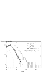
FIG. 3.: The number of events for $\chi^{2}<2.5$, $\chi^{2}<1.5$ and $\chi^{2}<1.0$ as a function of SNR², and an analytic fitting to $\chi^{2}<1.5$. The fitting was determined between SNR²=35 and 50. This fitting gives the number of events larger than SNR=7.2 and $\chi^{2}<1.5$ as 2.5. The $\chi^{2}<2.5$, $\chi^{2}<1.5$, and $\chi^{2}<1.0$ correspond to $10^{-3}\%$, $3.8\%$, and 46$\%$ false dismissal rate in Gaussian noise, respectively.

FIG. 4.: The detection probability of artificial signals of 1.4$M_{\odot}$ binaries as a function of distance in the case when the final thresholds were (SNR^∗,$\chi^{*2}$)= (7.2,1.5).

TABLE I.: (a) The preliminary second step thresholds used to determine the first step thresholds and the mesh spacing. (b) Optimized first step thresholds. (c) The first step thresholds used to derive the result of Fig.3 and 4. In both cases, the first step mesh area is 72 times larger than that of the second step.

	(a)		(b)		(c)
	$\rho^{*}$	$\chi^{*2}$	$\rho^{*}_{\rm 1st}$	$\chi^{*2}_{\rm 1st}$	$\rho^{*}_{\rm 1st}$	$\chi^{*2}_{\rm 1st}$
	9.3	1.0	8.0	1.3	7.0	1.3
	10.1	1.3	8.2	1.5	7.2	1.5
	10.6	1.5	8.5	2.0	7.5	2.0
	11.4	1.7	9.0	2.5	8.0	2.5
	12.1	2.0	10.2	3.0	9.2	3.0
	13.7	2.5

REFERENCES

- [1] A.Abramovici et al., Science 256, 325 (1992).
- [2] B.Caron et al., in Gravitational Wave Experiments, edited by E. Coccia, G. Pizzella, and F. Ronga, (World Scientific, Singapore, 1995).
- [3] K. Danzmann et al., in Gravitational Wave Experiments, edited by E. Coccia, G. Pizzella, and F. Ronga, (World Scientific, Singapore, 1995).
- [4] For details about the first data taking of TAMA300 project, see Gravitational Wave Detection II, (Proceedings of the 2nd TAMA workshop on Gravitational Wave Detection), (Univ. Acad. Press, Tokyo, 2000).
- [5] M. Ando et al., in preparation.
- [6] C. Alcock et al., Astrophys. J. 486, 697 (1997); C. Alcock et al., astro-ph/0001272.
- [7] T. Nakamura, M. Sasaki, T. Tanaka, and K.S. Thorne, Astrophys. J. Lett. 487, L139 (1997).
- [8] T.A. Apostolatos, Phys. Rev. D52, 605 (1995).
- [9] See e.g., LIGO-T970130-06-E, VIRGO-SPE-LAP-5400-102 (internal reports).
- [10] S.Telada et al., in ref.[4].
- [11] S.Telada et al., in preparation.
- [12] L. Blanchet, T. Damour, B. Iyer, C.M. Will, and A.G. Wiseman, Phys. Rev. Lett. 74, 3515 (1995); L. Blanchet, Phys. Rev. D54, 1417 (1996).
- [13] S. Droz, D.J. Knapp, E. Poisson, and B.J. Owen, Phys. Rev. D59, 124016 (1999).
- [14] B. Allen et al. Phys. Rev. Lett. 83, 1498 (1999).
-
[15]
For more details of test, see
B. Allen et al. ”GRASP software package”, release 1.9.4, section 6.24,
http://www.lsc-group.phys.uwm.edu/~ballen/grasp-distribution/ . - [16] Note the difference of this criterion to that discussed in S.D. Mohanty, Phys. Rev. D57, 630 (1998).
- [17] T. Tanaka, and H. Tagoshi, Phys. Rev. D62, 082001 (2000).
- [18] For example, Particle Data Group, Review of Particle Physics, Phys. Lett. B204 (1988), 81; ibid. Euro. Phys. J. C3, (1998), 172-177, and references cited there.