On line power spectra identification and whitening for the noise in interferometric gravitational wave detectors

Abstract

The knowledge of the noise Power Spectral Density of interferometric detector of gravitational waves is fundamental for detection algorithms and for the analysis of the data. In this paper we address both to the problem of identifying the noise Power Spectral Density of interferometric detectors by parametric techniques and to the problem of the whitening procedure of the sequence of data. We will concentrate the study on a Power Spectral Density like the one of the Italian-French detector VIRGO and we show that with a reasonable number of parameters we succeed in modeling a spectrum like the theoretical one of VIRGO, reproducing all its features.

We propose also the use of adaptive techniques to identify and to whiten on line the data of interferometric detectors. We analyze the behavior of the adaptive techniques in the field of stochastic gradient and in the Least Squares ones. As a result, we find that the Least Squares Lattice filter is the best among those we have analyzed. It optimally succeeds in following all the peaks of the noise power spectrum, and one of its outputs is the whitened part of the spectrum. Besides, the fast convergence of this algorithm let us follow the slow non stationarity of the noise. These procedures could be used to whiten the overall power spectrum or only some region of it. The advantage of the techniques we propose is that they do not require a priori knowledge of the noise power spectrum to be analyzed. Moreover the adaptive techniques let us identify and remove the spectral line, without building any physical model of the source that have produced them.

1 Introduction

1.1 Generalities

The detection of gravitational waves represents a major goal in contemporary Physics. A world-wide effort has been made in building detectors (especially ground-based long-arms detectors) with sensitivity enough to make astrophysical observations or, in a wider sense, to move in the field of gravitational astronomy [1, 2, 3]. The building of these large interferometers is now reaching the phase of data taking: TAMA (Japanese) [4] is already working; GEO (British/German) [5] will begin to take data next year; LIGO (U.S.A.) [6]in 2002; VIRGO (French/Italian) [7] in 2003. However, long test run of the Central Interferometer in VIRGO is foreseen during 2001, leading thus to a big amount of data to be analyzed: although these data are mainly for diagnostic purposes, they provide a very good opportunity to examine analysis techniques. In the following, even though we are referring to VIRGO antenna, our considerations can be in principle applied to all ground-based interferometric gravitational detectors. Generally speaking, all these detectors are Michelson interferometers with suitable technical additions in order to improve sensitivity (see [1, 8, 9] for exhaustive and up-to-date descriptions of physics and technology involved in building up interferometric gravitational antennae). A gravitational wave (GW) displaces in different way the far mirrors in the two arms, thus shifting the interference pattern at the beam-splitter; however, the best models we have for GW (astrophysics) sources are leading to a very small value for the wave amplitude on the earth [8, 9] requiring for its detection a spectral sensitivity of about $10^{-19}{\rm m}/\sqrt{\rm Hz}$ in a band of about 1 kHz, let’s say from few Hz to many hundreds of Hz. But to reach this nominal sensitivity is only the first challenge. In fact, other not minor challenges arise: the run of the antenna should be continuous because we are searching for rare time-limited events (supernovae bursts, coalescing binary systems) or, on the contrary, we have to integrate small continuous signals over long time (e.g. pulsars signals), while a very sensitive monitoring of the environment and instrument noise should be carefully and continuously done; when considering the low value of Signal to Noise Ratio (SNR), we are leading to foresee that large amount of data will be handled, very big computing power (TFLOPS) will be requested, large archiving capacity (TBYTES) will be prepared for storage and retrieval [10]. Finally, from a preliminary point of view for data treatment, which is indeed the argument of this paper, major challenge relies on the fact that the noise of GW detectors does not satisfy the simplifying assumptions of white noise, but expected noise is a colored broad-band background with some spectral (deterministic) peaks. Moreover the noise distribution could be non stationary and non Gaussian.

1.2 The problem

The large amount of data produced by gravitational wave detectors will be essentially noise and, hopefully, buried in noise there will be the signal we are looking for. As we already saw, ground-based interferometric detectors are sensible to a broad band frequencies (2-3Hz to more than 1kHz) in revealing relative displacement of test masses at the near and far extremities of interferometer arms due (possibly!) to GW signal, but unfortunately a lot of other factors can cause a similar displacement. The test masses are suspended to pendular structures in order to isolate them from seismic noise [14], but thermal noise of the suspension chain will cause a displacement of the mass [15]. Also shot noise and radiation pressure of the laser will move the mirrors [1, 16]. The physicists are working in modeling all possible causes of noise in the interferometer giving out a sensitivity curve of the apparatus [17, 18, 19, 20, 21, 22, 23]. This curve is limited at very low frequencies (few Hz and below) by seismic noise; in the middle band by thermal noise and at high frequencies (higher than $0.7-1$kHz) by shot-noise. In figure 1 is reported the predicted VIRGO sensitivity curve obtained as incoherent sum of all estimated noise contributions [24, 25]. This curve is characterized by a broad-band noise plus several very narrow peaks due to the violin modes of the suspensions wires, that will make the detection of a gravitational signal in this frequency band very difficult. For this reason efforts have been made in the preparation of the analysis of data for cutting  [26, 27, 28] out these resonances.

Figure 1: VIRGO sensitivity curve

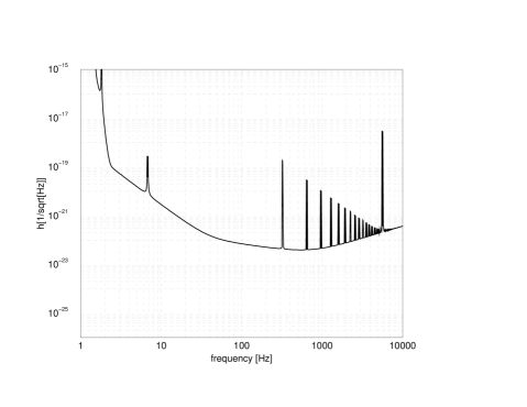
It is evident that the analysis of data to detect the gravitational signal requires an accurate knowledge of the noise, which means a statistical characterization of the stochastic process, evaluating its stationarity and its Gaussian nature, and in the case of local stationarity and Gaussian nature an accurate estimation of the Power Spectral Density (PSD).

The output of the interferometer will be surely non stationary over a long period of time, so we must be ready in following the changes in the PSD. A way to achieve this is to estimate the PSD on a chunk of data at different interval of time, using classical techniques [31, 35, 38]. We propose to use adaptive methods to follow on line the change in the feature of the spectrum in such a way to have at any desired instant the correct curve for the PSD.

If we are able in identifying the noise of our detector we can also apply the procedure of whitening of the data.

The goal of a whitening procedure is to make the sequence of data delta-correlated, removing all the correlation of the noise. Most of the theory of detection is in the frame of a wide-sense stationary Gaussian white noise, but in our problem the noise is surely a colored one and, in principle, there could be present non stationary and non Gaussian features. If we whiten the data, supposing hence to be in the frame of a stationary and Gaussian noise, we can apply the optimal algorithm detection[39].

For example, if we assume that the noise data which we are analyzing are stationary and Gaussian distributed and we suppose to know the waveform of our signal, then the optimal detection filter is the matching between our sequence of data and the Wiener filter:

$$M(t,\theta)=\int_{-\infty}^{\infty}e^{-2i\pi\nu t}\frac{h(\nu,\theta)}{S(\nu)}d\nu\,,$$ (1)

where $S(\nu)$ is the noise PSD and $h(\nu,\theta)$ is the template of the signal we are looking for, $\theta$ the parameters of the waveform. As it is evident from (1) the operation of whitening is implicitly done each time we apply the Wiener filter to detect a signal, because we weight the data with the inverse of PSD of noise: in such a way we have a ’whitened’ sequence to analyze.

Moreover when we are searching a transient signal of unknown form it is very important to have a whitened noise [12, 13]. The importance of whitening data is also linked to the possibility of reducing their dynamical range [37, 36].

The aim of this paper is to show how to identify the noise PSD and how to whiten the data produced by an interferometric detector before applying any algorithm detection.

In the section 2 we underline the advantages in parametric modeling; in section 3 we show the whitening techniques based on a lattice structure. In section 4 we report the application of PSD fitting and data whitening on VIRGO-like simulated data. In section 5 we introduce the theory of adaptive filters based on stochastic and least squares methods, and its application to VIRGO-like data: for this we compare their performances on simulated data.

2 Parametric Modeling

The advantages of parametric modeling with respect to the classical spectral methods are described in an exhaustive way in reference [31]. We want here to underline that the kind of analysis we have to perform can take advantage from these methods for two main reason. First of all we can achieve a better resolution in the estimation of PSD, because we can use in a better way the information of the autocorrelation function. In fact we suppose that the process we are analyzing is governed by a dynamical law and we can use the knowledge of autocorrelation function until a certain lag and then extrapolate its value under the dynamical hypothesis we made. Moreover we may compress the information of the PSD in a restricted number of parameter and not in the full autocorrelation function. This can help, for example, if we want to create a data base of noise sources.

In this context we want to talk about parametric modeling also because it offers the possibility to write down a linear whitening filter and to build in a fast way simulated data on which we perform our tests of whitening filter.

We work in the field of rational functions to fit the theoretical PSD. We will show that it is possible to obtain a fit of the theoretical PSD of an interferometer output like the one of VIRGO with an autoregressive moving average (ARMA) or autoregressive (AR) model[29, 30, 32], then we will use the data we can generate in this way, to test the whitening algorithms we propose.

2.1 ARMA and AR models

The procedure to estimate the PSD using parametric modeling is based on three steps:

1. select the appropriate model for the process;

2. estimate the model parameters from the given data;

3. use these parameters in the theoretical power spectrum density for the model.

Once we have the parameters which make the fit we use them to generate noise data to perform our tests.

A general process described by a ARMA(P,Q) model, being $P$ the number of poles and $Q$ the number of zeros, satisfies the relation:

$$x[n]=-\sum_{k=1}^{P}a[k]x[n-k]+\sum_{k=0}^{Q}b[k]w[n-k]$$ (2)

and its transfer function is given by

$${\mathcal{H}}(z)=\frac{{\mathcal{B}}(z)}{{\mathcal{A}}(z)}\,,$$ (3)

where${\mathcal{A}}(z)=\sum_{k=0}^{P}a[k]z^{-k}$ and ${\mathcal{B}}(z)=\sum_{k=0}^{Q}b[k]z^{-k}$ .

The PSD of the ARMA output process is

$$P_{ARMA}(f)=\sigma^{2}|\frac{B(f)}{A(f)}|^{2}\,,$$ (4)

$\sigma$ being the variance of driven white noise $w$, $A(f)={\mathcal{A}}(2\pi if)$ and $B(f)={\mathcal{B}}(2\pi if)$. An autoregressive process AR(P) is governed by the relation

$$x[n]=-\sum_{k=1}^{P}a[k]x[n-k]+w[n]\,,$$ (5)

and its PSD for a process of order $P$ is given by

$$P_{AR}(f)=\frac{\sigma^{2}}{|1+\sum_{k=1}^{P}a_{k}\exp(-i2\pi kf)|^{2}}$$ (6)

Once we selected the model for our process, we need to find the parameters for this model. The parameters of the ARMA model are linked to the autocorrelation function of the process by the Yule-Walker equations[31]. In the general case of an ARMA process we must solve a set of non linear equations while, if we specialize to an AR process, that is an all-poles model, the equations to be solved to find the AR parameters become linear.

The relationship between the parameters of the AR model and the autocorrelation function $r_{xx}(n)$ is given by the Yule–Walker equations

$$r_{xx}[k]=\left\{\begin{array}[]{ll}-\sum_{l=1}^{P}a_{l}r_{xx}[k-l]&\mbox{for}\,\,k\geq 1\\ -\sum_{l=1}^{P}a_{l}r_{xx}[-l]+\sigma^{2}&\mbox{for}\,\,k=0\,.\end{array}\right.$$ (7)

The problem of determining the AR parameters is the same of that of finding the optimal “weights vector” ${\mathbf{w}}=w_{k}$, for $k=1,...P$ for the problem of linear prediction [31]. In the linear prediction we would predict the sample $x[n]$ using the $P$ previous observed data ${\mathbf{x}}[n]=\{x[n-1],x[n-2]\ldots x[n-P]\}$ building the estimate as a transversal filter:

$$\hat{x}[n]=\sum_{k=1}^{P}w_{k}x[n-k]\,.$$ (8)

We choose the coefficients of the linear predictor by minimizing a cost function that is the mean squares error $\epsilon={\mathcal{E}}[e[n]^{2}]$ (${\mathcal{E}}$ is the expectation operator ), being

$$e[n]=x[n]-\hat{x}[n]$$ (9)

the error we make in this prediction and obtaining the so called Normal or Wiener-Hopf equations

$$\epsilon_{min}=r_{xx}[0]-\sum_{k=1}^{P}w_{k}r_{xx}[-k]\,,$$ (10)

which are identical to the Yule–Walker equations with

$$w_{k} = -a_{k}$$ (11)

$$\epsilon_{min} = \sigma^{2}$$ (12)

This relationship between AR model and linear prediction assures us to obtain a filter which is stable and causal [31]. It is this relation between AR process and linear predictor that becomes important in the building of whitening filter.

2.2 Durbin algorithm and lattice structure

A method of solving the Yule–Walker equation is the Durbin algorithm [34]. Let us suppose the process being an autoregressive one of order $P$.

The strategy of this method is to assume that the optimal $(P-1)$th order filter has previously been computed, and then to calculate the optimal $P$th order filter based on this assumption. To accomplish the algorithm we perform a loop on the order of the process for $1\leq j\leq P$. We initialize the mean squares error as $\epsilon_{0}=r_{xx}[0]$ and then we begin the iteration on the loop, introducing the reflection coefficients $k_{p}$ [38] at the stage $p$ , which are linked to the autocorrelation function $r_{xx}$ and to the $a_{j}$ parameters of the filter at the stage $p-1$ by the relation :

$$k_{p}=\frac{1}{\epsilon_{p-1}}\left[r_{xx}[p]-\sum_{j=1}^{p-1}a^{(p-1)}_{j}r_{xx}[p-j]\right]\,.$$ (13)

So the loop for $1\leq j\leq P$ proceeds in the following way:

• estimation of the reflection coefficient

  $$k_{j}=\frac{1}{\epsilon_{j-1}}\left[r_{xx}[j]-\sum_{i=1}^{j-1}a^{(j-1)}_{i}r_{xx}[j-i]\right]\,.$$ (14)

• at the $j$th stage the AR parameter of the model is equal to the $j$th reflection coefficient

  $$a_{j}^{(j)}=k_{j}\,,$$ (15)

• the other parameters are updated in the following way:

For $1\leq i\leq j-1$

$$a_{i}^{(j)}=a_{i}^{(j-1)}-k_{j}a_{j-i}^{(j-1)}$$ (16)

$$\epsilon_{j}=(1-k_{j}^{2})\epsilon_{j-1}$$ (17)

• At the end of the $j$ loop, when $j=P$, the final AR parameters are

  $$a_{j}=a_{j}^{(P)},\qquad\sigma^{2}=\epsilon_{P}\,.$$ (18)

3 Whitening Filter

3.1 Link between AR model and whitening filter

The tight relation between the AR filter and the whitening filter is clear in the figure 2. The figure describes how an AR process colors a white process at the input of the filter if you look at the picture from left to right. If you read the picture from right to left you see a colored process at the input that pass through the AR inverse filter coming out as a white process.

Figure 2: Whitening filter and AR filter.

When we find the $P$ parameters that fit a PSD of a noise process, what we are doing is to find the optimal vector of weights that let us reproduce the process at the time $n$ knowing the process at the $P$ previous time. All the methods that involves this estimation try to make the error signal (see equation (9) ) a white process in such a way to throw out all the correlation between the data (which we use for the estimation of the parameters).

The Durbin algorithm introduces in a natural way the Lattice structure for the whitening filter.

We show how the reflection coefficients $k_{p}$ are used to build a lattice whitening filter. Let us suppose to have a stochastic Gaussian and stationary process $x[n]$ which we modeled as an autoregressive process of order $P$. We define the forward error (FPE) for the filter of order $P$ in the following way

$$e_{P}^{f}[n]=x[n]+\sum_{k=1}^{P}a_{k}^{(P)}x[n-k]\,,$$ (19)

where the coefficients $a_{k}$ are the coefficients for the AR model for the process $x[n]$. The FPE represents the output of our filter. We can write the $zeta$ transform for the FPE at each stage $p$ for the filter of order $P$ as

$$FPE(z)=F_{p}^{f}[z]X[z]=\left(1+\sum_{j=1}^{p}a_{j}^{(p)}z^{-j}\right)X[z]\,.$$ (20)

At each stage $p$ of the Durbin algorithm the coefficients $a_{p}$ are updated as

$$a_{j}^{(p)}=a_{j}^{(p-1)}+k_{p}a_{p-j}^{(p-1)}\qquad 1\leq j\leq p-1\ .$$ (21)

If we use the above relation for the transform $F_{p}^{f}[z]$, we obtain

$$F_{p}^{f}[z]=F_{p-1}^{f}[z]+k_{p}\left[z^{-p}+\sum_{j=1}^{p-1}a_{p-j}^{(p-1)}z^{-j}\right]\ .$$ (22)

Now we introduce in a natural way the backward error of prediction BPE

$$F_{p-1}^{b}[z]=z^{-(p-1)}+\sum_{j=1}^{p-1}a_{p-j}^{(p-1)}z^{-(j-1)}\ .$$ (23)

In order to understand the meaning of $F_{p}^{b}[z]$ let us see its action in the time domain

$$F_{p-1}^{b}[z]x[n]=e_{p-1}^{b}[n]=$$ (24)

$$x[n-p+1]+\sum_{j=1}^{p-1}a_{p-j}^{(p-1)}x[n-j+1]\,.$$

So $e_{p-1}^{b}[n]$ is the error we make, in a backward way, in the prediction of the data $x[n-p+1]$ using $p-1$ successive data $\{x[n],x[n-1],\ldots,x[n-p+2]\}$.

We can write the eq. (22) using $F_{p-1}^{b}[z]$. Let us substitute this relation in the z-transform of the filter $F_{p}^{f}[z]$

$$F_{p}^{f}[z]=F_{p-1}^{f}[z]+k_{p}F^{b}_{p-1}[z].$$ (25)

In order to know the FPE filter at the stage $p$ we must know the BPE filter at the stage $p-1$.

Also for the backward error we may write in a similar way the relation

$$F_{p}^{b}[z]=z^{-1}F_{p-1}^{b}[z]+k_{p}F_{p-1}^{f}[z]\ .$$ (26)

The equations (25) (26) represent our lattice filter that in the time domain could be written

$$e_{p}^{f}[n] = e_{p-1}^{f}[n]+k_{p}e_{p-1}^{b}[n-1]\,,$$ (27)

$$e_{p}^{b}[n] = e_{p-1}^{b}[n-1]+k_{p}e_{p-1}^{f}[n]\,.$$ (28)

In figure 3 is showed how the lattice structure is used to estimate the forward and backward errors.

Figure 3: Lattice structure for Durbin filter.

Using a lattice structure we can implement the whitening filter following these steps:

• estimate the values of the autocorrelation function $\hat{r}_{xx}[k],\mbox{$0\leq k\leq P$}$ of our process $x[n]$;

• use the Durbin algorithm to find the reflection coefficients $k_{p},\mbox{$1\leq p\leq P$}$;

• implementation of the lattice filter with these coefficients $k_{p}$ initiating the filter $e_{0}^{f}[n]=e_{0}^{b}[n]=x[n]$.

In this way the forward error at the stage $P$-th is equivalent to the forward error of a transversal filter and represents the output of the whitening filter.

The procedure of whitening will be accomplished before applying the algorithms for the detection of gravitational signal of different wave forms. The level of whiteness of the data needed for the various algorithms could be different. It is important to have a common language and to assign a parameter which characterizes the performance of whitening filter. We want now to introduce this parameter that let us quantify the level of whiteness of data at the output of whitening filter.

3.2 The “whiteness” of data: measure of flatness of PSD

The spectral flatness measure for a PSD is defined as[31]

$$\xi=\frac{\exp(\frac{1}{N_{s}}\int_{-N_{s}/2}^{N_{s}/2}\ln(P(f))df)}{\frac{1}{N_{s}}\int_{-N_{s}/2}^{N_{s}/2}P(f)df}$$ (29)

where the integral is extended in the bandwidth of Nyquist frequency; this parameter satisfies

$$0\leq\xi\leq 1$$ (30)

If $P(f)$ is very peaky, then $\xi\simeq 0$, if $P(f)$ is flat than $\xi=1$.

With th definition 29 the flatness for a process at the output of a whitening filter built with a minimum phase filter (as the AR filter is) is

$$\xi_{e}=\xi\frac{r_{xx}[0]}{r_{ee}[0]},$$ (31)

where $r_{xx}[0]$ and $r_{ee}[0]$ are the values of the autocorrelation function of the process before and after the whitening procedure, and $\xi$ is the value of flatness for the initial sequence [31].

4 Results on simulated VIRGO-like noise data

We want to investigate the performance of the Durbin filter in fitting the VIRGO PSD and in whitening the simulated output of this interferometer.

We can simulate the data as AR or ARMA process [29], by fitting the theoretical PSD as an AR or ARMA model. If we simulate the data as an AR process and fit them with an AR model, the number of parameters we must use will be small. In the real situation the output of interferometer will not be an AR process. This does not mean that we cannot ever fit the data as an AR process, but that probably we need a greater number of parameters. In order to be closest to the real situation we use an ARMA fit to the theoretical PSD and we performed the tests following the steps:

• ARMA fit to theoretical VIRGO-like noise PSD

• Generation of noise data with the ARMA parameters

• realization of one process of noise

• P order selection for the AR fit to the realization of the noise

• Durbin(P) whitening filter.

4.1 The VIRGO noise power spectrum

We consider a theoretical curve for a VIRGO-like power spectrum in which shot noise and thermal noise of pendulum, mirrors and violin modes are present:

$$S(f)=\frac{\displaystyle S_{1}}{\displaystyle f^{5}}+\frac{\displaystyle S_{2}}{\displaystyle f}+S_{3}\left(1+\left(\frac{f}{f_{K}}\right)^{2}\right)+S_{v}(f)$$ (32)

where

$$f_{K} = 500{\rm Hz}\qquad\mbox{shot noise cut frequency}$$ (33)

$$S_{1} = 1.08\cdot 10^{-36}\qquad\mbox{pendulum mode}$$ (34)

$$S_{2} = 0.33\cdot 10^{-42}\qquad\mbox{mirror mode}$$ (35)

$$S_{3} = 3.24\cdot 10^{-46}\qquad\mbox{shot noise}$$ (36)

The contribute of violin resonances is given by

$$S_{v}(f)=\sum_{n}\frac{1}{n^{4}}\frac{f_{1}^{(c)}}{f}\frac{C_{c}\phi_{n}^{2}}{\left(\displaystyle\frac{1}{n^{2}}\frac{f^{2}}{f_{1}^{(c)2}}-1\right)^{2}+\phi_{n}^{2}}+(c\leftrightarrow f)$$ (37)

where we take into account the different masses of close and far mirrors, being

$$f_{n}^{(c)}=n\cdot 327{\rm\,Hz}\qquad f_{n}^{(f)}=n\cdot 308.6\rm\,Hz$$ (38)

$$C_{c}=3.22\cdot 10^{-40}\qquad C_{f}=2.82\cdot 10^{-40}\qquad\phi_{n}^{2}=10^{-7}$$ (39)

The difference between far and close masses leads to the presence of double violin peaks, as we can see in figure 4, where we have plotted the spectrum obtained with a sampling frequency $f_{s}=4096\rm\,Hz$.

We suppose to explore the band of frequencies from $10$Hz to $\sim 2000$ Hz, where it is most probable to find a gravitational signal, choosing a sampling frequency of $4096$Hz. The low frequency part of the spectrum has been filtered to cut the tail of the thermal noise. We used a second order high pass filter with spectral density [42]:

$$|H(\omega)|^{2}=\frac{1}{1+\epsilon^{2}_{pass}\left(\frac{\displaystyle\cot(\omega/2)}{\displaystyle\cot(\omega_{pass}/2)}\right)^{2N}}\,$$ (40)

with the following values

$$\epsilon_{pass}=1000\,,\qquad N=2\,,\qquad\omega_{pass}=3\pi\,.$$ (41)

4.2 Data simulation

First of all we make an ARMA fit to the theoretical PSD with the techniques used in [29]. We choose to use $P=32$ and $Q=32$ parameters then we simulated the data in the time-domain using the relation 2, with a pre-heating techniques as described in [31].

Figure 4: ARMA(32,32) fit to theoretical VIRGO PSD

Figure 5: PSD of VIRGO-like simulated data.

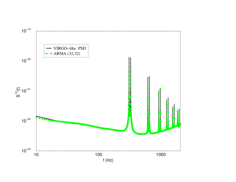
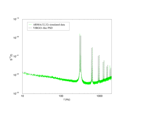
In figure 4 we plot the theoretical VIRGO PSD and the ARMA(32,32) fit, while in figure 5 we show the PSD obtained as an averaged periodogram on $50$ realizations of the process for simulated data. As it is evident the fit is good and we can suppose the time-domain data well represent the expected Gaussian and stationary noise process for VIRGO interferometer.

4.3 Order Selection

The idea of the whitening filter is that the process we analyze is an autoregressive one and that once we have the AR parameters we can use them in the filter of figure 2.

In general we don’t know the order of our process, even if we suppose that it is an AR one. If it is an AR of order P, and we use an order $p<P$, the fitted spectrum will be smoother than the original one; if we choose an order $p>P$, there may be spurious peaks in the spectrum. In both cases the whitening will be not good.

If our process is not AR, the number of parameters could be in principle infinite. We must then fix a criterion that let us select the right order of the process, or at least the best one.

We used the classical order selection criteria [31, 35], that is the Akaike information criterion (AIC), the forward prediction error (FPE) the Parzen’s criterion (CAT) and the minimum description length (MDL) one

$$AIC(P) = N\log\epsilon(P)+2P\,\,,$$ (42)

$$FPE(P) = \epsilon(P)\frac{N+P+1}{N-P-1}\,\,,$$ (43)

$$CAT(P) = \left(\frac{1}{N}\sum_{j=1}^{P}\frac{N-j}{N\epsilon_{j}}\right)-\frac{N-P}{N\epsilon_{P}}\,\,,$$ (44)

$$MDL(P) = N\log\epsilon(P)+P\log N\,\,,$$ (45)

where $\epsilon(P)$ is the mean square error at the order $P$ and $N$ is the length of data. In literature the MDL criterion is considered the best among them, because it is robust with respect to the length of the sequence, while the others depend a lot on N[35]. Suppose, as in the real situation, we have not access to the theoretical PSD of our noise process and we want to estimate the best order of the whitening filter. We can use a single realization of process, i. e. a sequence of N-data to estimate the autocorrelation function and apply the selection order criteria to it. The results of these criteria are reported in table 1.

Table 1: Minimum of order selection criteria on a single sequence for $1$ minute of ARMA simulated VIRGO data.

• MDL	AIC	FPE	CAT
  338	626	626	681

The best order to whiten the data is given by the MDL criterium [31][35] which produces an order of $338$ parameters.

This number is an indicative one. We can choose to build a higher order filter to be sure to have whitened data at the output of the filter. We choose to adopt the number of parameters of MDL criterion and we test the flatness of the spectrum at the output of the Durbin filter measuring the value of $\xi.$

All the order selection criteria give an estimation of the number of parameters such that the output of the whitening filter has the maximum value of $\xi$.

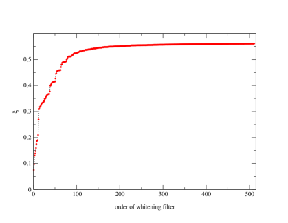
In figure 6 we report $\xi$ versus the number of parameters of whitening filter. The value of $\xi$ for very low order $P$ is small and, as expected, it increases with the order $P$ until it converges to a plateau around $P\sim 300$. So we deduce that our choice of $P=338$ is a good estimation of whitening filter order.

Figure 6: Behavior of $\xi$ with respect to the order P for the VIRGO-like simulated data.

4.4 Results of Durbin whitening filter on simulated VIRGO-like noise data

Figure 7: Exit of Durbin whitening filter.

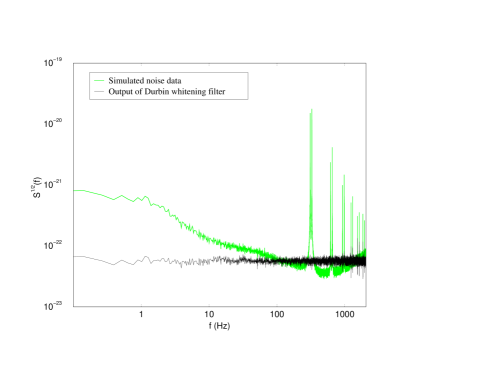
In figure 7 we plotted the averaged PSD on $100$ realizations of input noise and of the output of Durbin whitening filter. The results are good even if there are some residual lines at the high frequencies.

We can do a better whitening if we take a higher order whitening filter, but we must pay a higher computational cost itself, because it is proportional to the order P of the filter. The level of whitening we choose to perform depends on the requests for the detection algorithms.

Figure 8: Measure of flatness for simulated noise process and outputs of whitening filters.

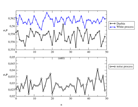
In figure 8 we report the measure of $\xi$ in a set of realizations of the process of simulated noises. The values are reported before any application of whitening filter and after the application of ’static’ whitening filter. We estimate the value of flatness also for a simulated white noise process to check the goodness of the whitening filters.

As we can see in figure 8, in a single realization the value of flatness is high but not equal to $1$, because of variance of the estimate of periodogram. On the other hand in the averaged periodogram the value of $\xi$ is very close to $1$ as we can read in table 2.

Table 2: Flatness on averaged PSD at the input and the outputs of whitening filter for VIRGO-like simulated data.

• Simulated noise	Durbin	White process
  0.050	0.983	0.989

5 Adaptive filters

Since now we showed filters which estimate the parameters to be used in the whitening filter from the autocorrelation function or PSD, i.e. these filters use a priori information about the statistics of the data to be analyzed. Now we want to investigate the behavior of filters which are self-designing [33]. These filters estimate the parameters directly from data adjusting them by using as feed-back the signal obtained by the minimization of a cost function of the error signal. In figure 9 is reported the scheme of an adaptive filter for system identification. In our case the plant is represented by the parameters which fit the PSD of data. The implementation of an adaptive filter follows two steps: the filtering of the input data and the adjustment of the filter parameters with which we process the data to the next iteration.

Figure 9: Scheme of adaptive filter for system identification.

The filters parameters are updated by minimizing a cost function. The way in which we build this cost function distinguishes the adaptive methods as [33, 34]:

• methods of stochastic gradient,

• least squares methods.

To the first class belong the algorithms whose cost function is the mean square error ${\cal E}[e^{2}[n]]$, where $e[n]$ is the difference between the function we desire to find and the output of our filter. We talk of stochastic methods because the cost function is a statistical measure of the error. In the second class the cost function is the weighted sum of the square errors $e^{2}[n]$. These methods could be implemented with a block estimation or with a recursive one (Recursive Least Squares). For the block estimation a block of data is acquired and then the least square algorithm is applied, while in the recursive one the least squares methods should be implemented in a recursive way.

In order to be able to obtain on line the fit to the PSD, we will use only the recursive kind. We used the Gradient Adaptive Lattice (GAL), the Recursive Least Squares (RLS) and the Least Squares Lattice (LSL). The technical details of these algorithms are described in references  [33] [34].

The next sections of this paper are organized in two parts: in the first part we make a comparison of the GAL, RLS and LSL methods to fit a VIRGO-like noise PSD. For this we simulated the data as an autoregressive process; we consider the parameters we use in the simulation as the true values and we check the capability of the algorithm in converging towards these values. In the second part, we will report the application of the LSL methods as whitening filter on data simulated as ARMA process, to show that even in the case of a process which is not an autoregressive one, we succeed in fitting it with an AR with a low number of parameter and in obtaining a whitened PSD.

To check the performances of these algorithms we use the following scheme:

• modeling of the VIRGO as an AR process by Durbin algorithm;

• data simulation of the noise process following the AR relation

  $$x[n]=-\sum_{k=1}^{P}a_{k}x[n-k]+w[n]\,;$$ (46)

• implementation of adaptive algorithm without any information on the input sequence of data;

• comparison between the estimated PSD and the obtained one.

It is fundamental to test the time convergence of the algorithms to compare them with the typical times of non stationarities. To this goal we measure the number of iterations by which the measured values reach the true values of the parameters. This is done in the case of AR simulation, where the two quantities are comparable.

If we simulate the process as an AR one the MDL order selection criterion gives as best order the value $292$. We select this one to perform our simulation and our tests.

6 Application to VIRGO-like simulated data

We applied the GAL method on simulated data to verify its capability in identifying the VIRGO-like noise power spectrum.

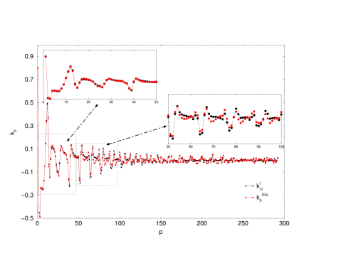
The convergence is reached after $2$ minutes of data, but not for all the coefficients, as it is evident in figure 10, where we plotted all the $292$ coefficients and zoomed the regions corresponding to $p=1,2\ldots,50$ e $p=50,51,\ldots,100$. After the first $50$ points there is an evident discrepancy between the simulated and the estimated reflection coefficients. This causes the non convergence of the AR parameters even for the first two coefficients (see figure 11).

Figure 10: Comparison between the reflection coefficients estimated by Durbin and GAL algorithms

Figure 11: Convergence of the AR coefficients to true values after $4$ minutes of data

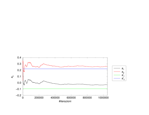
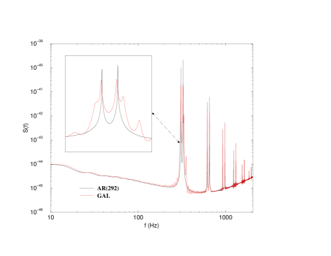
Even if we use a larger number of iteration, the convergence is not reached. This is reflected in the estimation of the PSD, as you can see in the figure 12 where the estimated GAL PSD is reported. The violin peaks are reproduced only in a rough way. This is due to the kind of cost function we used to find the reflection coefficient, that is optimal only in a statistical sense and not for the actual value of the error function.

Figure 12: GAL fit to the VIRGO PSD

7 Least Square based methods

The Least Squares based methods build their cost function using all the information contained in the error function at each step, writing it as the sum of the error at each step up to the iteration $n$ :

$$\epsilon[n]=\sum_{i=1}^{n}\lambda^{n-i}e^{2}(i|n)\,,$$ (47)

being

$$e(i|n)=d[i]-\sum_{k=1}^{N}x_{i-k}w_{k}[n],$$ (48)

where $d$ is the signal to be estimated, $x$ are the data of the process and $w$ the weights of the filter. We introduced the forgetting factor $\lambda$ that let us tune the learning rate of the algorithm. This coefficient can help when there are non stationary data in the data and we want that the algorithm have a short memory. If we have stationary data we fix $\lambda=1$.

There are two ways to implement the Least Squares methods for the spectral estimation: in a recursive way (Recursive Least Squares or Kalman Filters) or in a Lattice Filters using fast techniques [34]. The first kind of algorithm, examined in [30], has a computational cost proportional to the square of the order of filter, while the cost of the second one is linear in the order $P.$

7.1 RLS: application to VIRGO noise data

We used about $1$ minute of data, choosing a sampling frequency of $4096\rm\,Hz$.

In this transversal filter we update directly the weights, without estimating the reflection coefficients. In figure 13 we report the convergence curves for the first two coefficients $a_{1}$, $a_{2}$ and for the last two coefficients $a_{291}$, $a_{292}$ estimated by the RLS algorithms and the corresponding ’true’ values $a^{t}_{1}$, $a^{t}_{2}$, $a^{t}_{291}$ and $a^{t}_{292}$.

Figure 13: Convergence of the first two and the last two AR parameters for RLS filter.

Figure 14: Simulated AR parameters and estimated coefficients by RLS algorithm

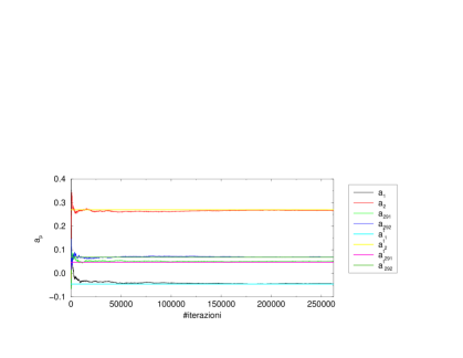
The RLS algorithm converges to the true value of the parameters, and its convergence time its of the order of $30$ sec.

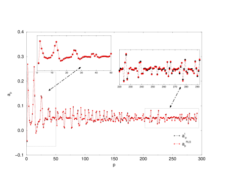
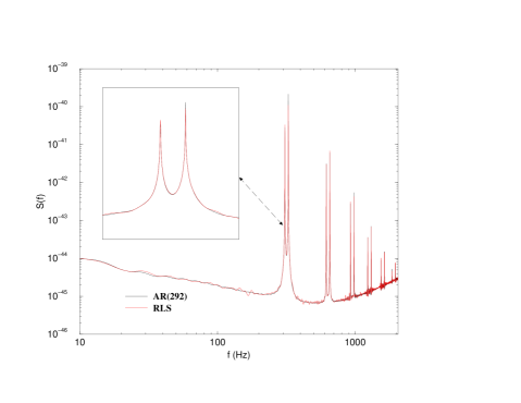
In figure 14 we report the $292$ parameters for the AR model estimated with RLS after $1$ minute of iterations and the corresponding true values. In the zooms we can see the first $50$ and the last $70$ coefficients. There is a small discrepancy in the estimations of the last coefficients, but this doesn’t affect the fit of the original PSD as it is evident in figure 15, where all the spectral features are well reproduced.

Figure 15: RLS fit to the VIRGO PSD

7.2 LSL: application to VIRGO-like noise data

The computational cost of RLS is prohibitive for an on line implementation. Moreover its structure is not modular as for the GAL algorithm, thus forcing the choose of the order $P$ once for all. The algorithm with a modular structure like that of the lattice offers the advantages of giving an output of the filter at each stage $p$, so in principle we can change the order of the filter by imposing some criteria on its output. On the contrary the Least Square Lattice filter is a modular filter with a computational cost proportional to the order $P$.

We introduced for the LSL filter the forward and backward reflection coefficients. These in principle could have different values if the sequence is not stationary, but we simulate the VIRGO-like noise data as a stationary process, therefore $k_{p}^{f}=k_{p}^{b}=k_{p}$. Moreover we use the pre-windowed case $\lambda=1$.

We used always $1$ minute of data with a sampling frequency of $4096\rm\,Hz$. The AR parameters have been estimated from the reflection coefficients using the relation (21).

The error $e_{p}^{f}$ at the last stage is the whitened sequence of the input data. So at the output of LSL filter we find the parameter for the estimation of the AR fit to VIRGO PSD and the whitened sequence of data.

As we expected, the performances are similar to the ones of RLS filter and the convergence is reached after about $30\sec$ of data. This behavior is satisfied by all the coefficients $a_{p}$ as it is evident in figure 16 where we plotted all the coefficients of simulation and the estimated ones.

Figure 16: LSL estimated AR parameters.

Figure 17: LSL fit to the VIRGO-like noise PSD.

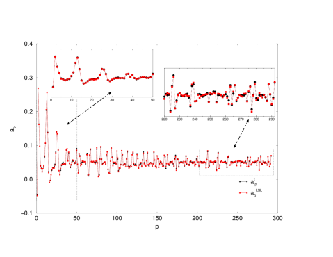
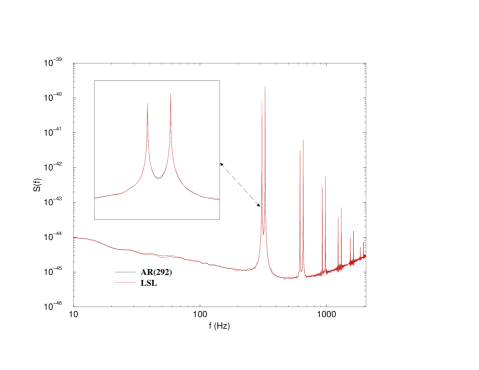
We zoomed on to the first $50$ coefficients and to the last $70$ ones. As for the RLS filter there is a small discrepancy only for the last coefficients, but this does not affect the spectral estimation as reported in figure 17, where all the violin peaks are well reproduced. In only one minute of data we succeeded in identifying an AR model with $292$ parameters. If we think about not stationarity noise with characteristic time of one hour, we are sure to obtain on line the right estimation of the PSD, and the right whitened sequence.

In figure 18 we reported the PSD of the sequence $e_{P}^{f}[n]$ obtained as averaged periodogram on $100$ noise simulations.

Figure 18: Exit of LSL whitening filter.

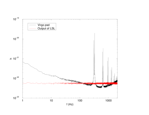
It is clear that the LSL is a good whitening filter and it offers the advantages, with respect to the Durbin one, of being adaptive and of working without estimating before the autocorrelation function from the data.

7.3 LSL statistics

In order to evaluate the goodness of an estimator we verify if it is an unbiased one and if it satisfies the Cramer-Rao bound which for the AR parameters is [31]

$$var(\hat{a}_{i})\geq\frac{\sigma^{2}}{N}[{\bf R}_{xx}^{-1}]_{ii}\qquad\mbox{$i=1,2,\ldots p$}\,,$$ (49)

and

$$var(\hat{\sigma})\geq\frac{2\sigma^{2}}{N}\,.$$ (50)

Figure 19: Bias for the AR parameters.

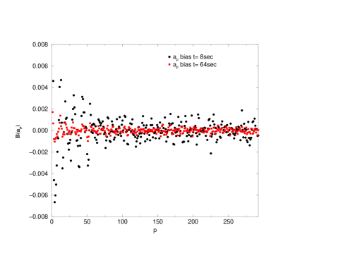
We fixed $1$ minute of data as the maximum length for $N$ and we estimated the bias for the parameters $a_{p}$. The statistical quantities have been evaluated as averages on $100$ realizations of the process. In figure 19 we report the bias for each AR parameter

$$B(a_{p})={\cal E}[\hat{a}_{p}]-a^{t}_{p}\$$ (51)

estimated at two different times: the first at $8$s of data and the second at $64$s. It is evident that the quantities $B(a_{p})$ are equals to zero after $1$ minute of data.

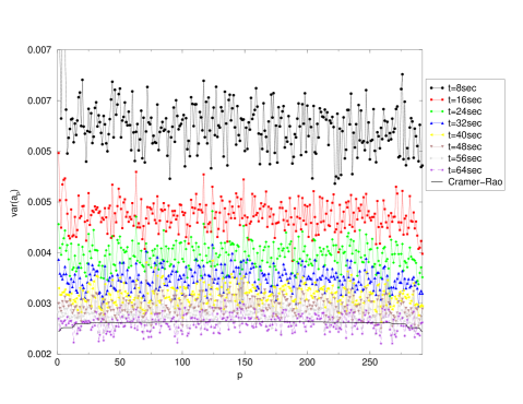
Now to evaluate the efficiency of the estimator LSL we verify that the variance for the estimated coefficients $a_{p}$ reaches the Cramer-Rao (eq. (49)) limit.

In figure 20 we report the estimated variance for the coefficients $a_{p}$ at the output of LSL filter and the theoretical Cramer-Rao bound. The variance has been estimated at steps of time growing until the limit of $64$s. It is evident that its values become smaller and smaller increasing the number of iteration and that it reaches the Cramer-Rao theoretical limit [30].

Figure 20: Cramer-Rao bound for LSL parameters.

7.4 If the noise is not a AutoRegressive process

Suppose that our process is not an autoregressive one: does the LSL work well in this situation? To verify this we simulated, as in the Durbin case, the data as an ARMA process and test the LSL on this sequence of data. The optimal order for the AR fit to these data now is $338$, so we use this order for the LSL final stage.

In figure 21 we plotted the PSD of the simulated data and at the output of the LSL filter averaged on $100$ realizations.

Figure 21: Exit of LSL whitening filter.

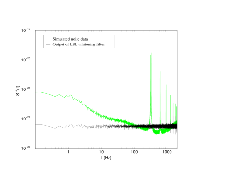
It is evident that the LSL succeeded in whitening also the ARMA sequence, even if we use an AR fit. In table 3 we reported the values of flatness for the outputs of Durbin and LSL filter.

Table 3: Flatness on averaged power spectra at the input and the outputs of whitening filter for VIRGO-like simulated data.

• Simulated noise	Durbin	LSL	White process
  0.050	0.983	0.984	0.989

The values of flatness for LSL and Durbin whitening filter are similar, even if it is evident that LSL whitens better than Durbin filter. We think that this is related to the fact that the adaptive filters don’t need the previous estimation of autocorrelation function; in this way if we make a mistake in estimating the autocorrelation it will not propagate in the estimation of coefficients.

8 Conclusion

In this paper we addressed the problem of on-line identification of the parameters which fitted the PSD at the output of an interferometric detector like the VIRGO one. Moreover we face the problem of whitening on-line the sequence of data.

In this work we reviewed the Durbin and LSL whitening algorithms and we reported the results of whitening on VIRGO-like noise simulated data, showing that it is possible to obtain a whitened PSD. We verified that the LSL adaptive algorithm has a better performance with respect to the static algorithm so it could be useful if we have to face with non stationary data. It is important to note that in selecting the order of whitening filters it is crucial a good knowledge of the level of whiteness needed for the different signal detection algorithms. In fact we showed that the value of flatness tends to reach a plateau with respect to the number of parameters used in the whitening filters while the computational cost increases proportionally to the order of filter.

The procedure of whitening we described is a linear procedure that does not destroy any part of the data. It is a reversible process that can be updated to the level of whiteness we need. It is worth to note that the Durbin algorithm is a ’static’ procedure: we suppose to know that we are analyzing only noise and we fit the parameters to perform the whitening on the next sequence of data. In this way if in the next sequence of data there is a signal, we don’t white the signal even if we can modify its waveform. Note that we have under control the kind of changes we made to the signal, because we know the parameters of our whitening filter. Instead when we use the adaptive algorithms we could in principle let the algorithm learn also the signal buried in the noise, and whiten all the information about it, but the learning time of the algorithm we described is such that only a periodic signal can be captured by this algorithm. In an incoming paper we will report the tests we made on the whitening procedure applied to sequences of data containing gravitational signals [43].

The goodness of such filters as whitening filters has been already tested on data taken from prototype interferometer with very encouraging results [32, 44].

References

- [1] Saulson P R 1994 Fundamentals of Interferometric Gravitational Wave Detectors World Scientific Pub Co ISBN:9810218206
- [2] Schutz B 1999 Class. Quantum Grav., 16 p 131
- [3] Grishchuk L P et alPreprint astro-ph/0008481
- [4] Ando M et al2000 Proc. 3rd E. Amaldi Conference (New York: AIP Proceedings) p 128
- [5] Luck H et al2000 Proc. 3rd E. Amaldi Conference (New York: AIP Proceedings) p 119
- [6] Coles M W 2000 Proc. 3rd E. Amaldi Conference (New York: AIP Proceedings) p 101
- [7] Marion F 2000 Proc. 3rd E. Amaldi Conference (New York: AIP Proceedings) p 110
- [8] Blair D G (ed) 1993 The Detection of Gravitational Waves (Cambridge: Cambridge University Press)
- [9] Barone M, Calamai G, Mazzoni M, Stanga R, Vetrano F (Eds) 2000 Proceedings of the International Summer School on Experimental Physics of Gravitational Waves (Singapore: World Scientific Pub)
- [10] Owen B J and Sathyaprakash B S 1999 Phys Rev. D 60 p 22002
- [11] Brady P B and Schutz B F 1998 Phys. Rev. D, 57, p 2101
- [12] Pradier T et al2000 Int. J. Mod. Phys. D9 p 309
- [13] Pradier T et alPreprint gr-qc/0010037
- [14] Bradaschia C et al1990 Nucl. Instr. Meth. A 289 p 518
- [15] Cagnoli G. et al1999 Phys. Lett. A 255 p 230
- [16] Meers B J 1988 Phys. Rev. D 38 (8) p 2317
- [17] Thorne K. S. and Winstein C. J. 1999 Phys.Rev.D 60 082001
- [18] Hughes S. A and Thorne K. S. 1998 Phys.Rev.D 58 122002
- [19] Cella G. Cuoco E 1997 VIR-NOT-PIS-1390-099 (Internal Note)
- [20] Beccaria M et al1998 Classical and Quantum Gravity 15 p 3339
- [21] Cella G Off-line Subtraction of Newtonian Noise 1999 Proc. of 34 Rencontre de Moriond Conf. (In press)
- [22] Cagnoli G. et al1998 Phys. Lett. A 237 p 21
- [23] Braginsky V B Levin Y Vyatchanin S 1999 Measur. Sci.Tech. 10 p 598
- [24] Thanks to Michele Punturo who gave us this plot.
- [25] Cattuto C et al1999 (VIR-NOT-PER-1390-51) (Internal note)
- [26] Finn L S and Mukherjee S Preprint gr-qc/0005061
- [27] Sintes A M Schutz B F 1998 Proc.of the 2nd workshop on Gravitational Wave Data Analysis Edts. Davier M and Hello P Editions Frontières p 255
- [28] Chassande-Mottin E Dhurandhar S V Preprint gr-qc/0004075
- [29] Cuoco E Curci G 1997 Modeling a VIRGO-like noise spectrum. Note IVIR-NOT-PIS-1390-095 (Internal note)
- [30] Beccaria M Cuoco E Curci G 1997 Adaptive System Identification of VIRGO-like noise spectrum Proc. of 2nd Amaldi Conference World Scientific
- [31] Kay S 1988 Modern spectral estimation:Theory and Application Prentice Hall Englewood Cliffs
- [32] Cuoco E 2000 Whitening of noise power spectrum. Test on LIGO 40-meter interferometer data VIR-NOT-FIR-1390-145 (Internal Note)
- [33] Haykin S 1996Adaptive Filter Theory (Upper Saddle River: Prentice Hall)
- [34] Alexander S T 1986 Adaptive Signal Processing (Berlin: Springer-Verlag)
- [35] Hayes M H 1996Statistical Digital Signal Processing and Modeling Wiley
- [36] Allen B 1999 GRASP: a data analysis package for gravitational wave detection
- [37] Allen B Brady P 1997 Quantization noise in Ligo interferometer Ligo (Internal note)
- [38] Therrien C W 1992Discrete Random Signals and Statistical Signal Processing (Englewood Cliffs: Prentice Hall)
- [39] Zubakov L A Wainstein V D 1962 Extraction of signals from noise (Englewood Cliffs: Prentice Hall)
- [40] Parzen E 1977 An approach to Time series modeling: determining the order of approximating autoregressive schemes in “Multivariate Analysis” North Holland
- [41] Widrow B and Stearns S D 1985 Adaptive Signal Processing (Englewood Cliffs: Prentice Hall)
- [42] Orfanidis S J 1996 Introduction to Signal Processing (Englewood Cliffs: Prentice-Hall)
- [43] Work in progress
- [44] E. Cuoco et al Noise parametric identification and whitening for LIGO 40-meter interferometer data in preparation