The fate of chaotic binaries

Abstract

A typical stellar mass black hole with a lighter companion is shown to succumb to a chaotic precession of the orbital plane. As a result, the optimal candidates for the direct detection of gravitational waves by Earth based interferometers can show irregular modulation of the waveform during the last orbits before plunge. The precession and the subsequent modulation of the gravitational radiation depends on the mass ratio, eccentricity, and spins. The smaller the mass of the companion, the more prominent the effect of the precession. The most important parameters are the spin magnitudes and misalignments. If the spins are small and nearly aligned with the orbital angular momentum, then there will be no chaotic precession while increasing both the spin magnitudes and misalignments increases the erratic precession. A large eccentricity can be induced by large, misaligned spins but does not seem to be required for chaos. An irregular precession of the orbital plane will generate irregularities in the gravitational wave frequency but may have a lesser effect on the total number of cycles observed.

04.30.Db,97.60.Lf,97.60.Jd,95.30.Sf,04.70.Bw,05.45 ]

Merging black hole binaries are potent sources of gravitational waves and are among the most promising targets for direct detection by the future interferometric observatories. Black hole mergers, if sufficiently abundant, are likely to be the most common compact binary merger to be detected. If the black holes are rapidly spinning, then the orbit can be extremely irregular, even chaotic, bearing significant implications for gravitational wave searches [1, 2, 3, 4, 5, 6, 7]. An earlier Letter [2] identified chaos in relativistic, spinning binaries in a somewhat abstract discussion. In this article, the intention is instead to provide a more concrete discussion with less emphasis on formal chaos. What is observationally important is visibly irregular motion. Taking this attitude, a specific astrophysical model is followed through successive stages in order to gauge when irregular motion will occur within the LIGO/VIRGO bandwidth. Specifically, we investigate the orbits of a maximally spinning black hole with a lighter companion.

Certain binary star systems are fated to evolve into black hole binaries. The orbits of these long lived binaries have sufficient time to circularize before entering the LIGO/VIRGO bandwidth as angular momentum is lost to gravitational waves. An archive of circular templates is accruing for various binary parameters. Yet the merger rates of these evolved binaries are predicted to be too low to ensure detection by the first two generations of LIGO detectors. A more promising detection rate is predicted for dynamical binary black holes; that is, binaries formed by the dynamical capture of one black hole by another in dense stellar systems [8]. The merger rate is expected to be about $1.6\times 10^{-7}$/yr/Mpc³, which exceeds neutron star merger rates as well. Dynamically formed black hole binaries should have a distribution of eccentricities and short orbital periods with masses in the range of $\sim(5-15)M_{\odot}$ [8]. A binary with masses $m_{1}=15M_{\odot}$ and $m_{2}=5M_{\odot}$ for instance will emit gravitational waves with a frequency within the optimal LIGO bandwidth of $f\sim(10-10^{2})$ Hz for radial separations $r\mathrel{\hbox to0.0pt{\lower 3.0pt\hbox{$\mathchar 536\relax$}\hss}\raise 2.0pt\hbox{$\mathchar 316\relax$}}50m$ where units of total mass $m=m_{1}+m_{2}$ are used. These provide natural values for the mass and radii ranges to investigate. The heavier black hole is taken to have maximal spin $S_{1}=m_{1}^{2}$ (spin period $P\sim 3\times 10^{-4}s$ for a $15M_{\odot}$ black hole). Unlike pulsars, black holes are expected to essentially maintain the spin they are born with [9] through most of the inspiral. This canonical BH/BH pair can precess chaotically any time the trajectory transits near the underlying homoclinic orbits of Refs. [10]. Homoclinic orbits are purely relativistic, a consequence of nonlinearity, and unstable. They have the essential features for the onset of chaos [4, 10] when the bodies spin. Still, having said this, it is not clear that chaos will be confined to this region of phase space.

A BH/NS binary with typical parameter values of $m_{1}=10M_{\odot}$ and $m_{2}=1.4M_{\odot}$ follows trends similar to the BH/BH binaries. The explosive evolution of stellar progenitors which populate BH/NS pairs delivers large kicks to the objects and leads to large spin misalignments [11]. It is still unclear whether the population of such pairs is too sparse to expect a detection. Since it is only the mass ratio which enters the equations, either of these cases can be scaled to represent the dynamics of much more massive systems which will be visible to LISA [12].

We look for chaotic behaviour when energy is conserved and the radiation reaction is turned off. For an individual orbit, chaos manifests itself as the unpredictable precession of the orbital plane. When considering all possible orbits, chaos manifests itself as an extreme sensitivity of the orbital precession to initial conditions so two neighboring orbits may live out very different precessional histories. The implication is that there is a theoretical limit on how well we can predict the orbit and therefore the waveform of the emitted gravitational radiation [1, 2]. Dissipation from the emission of gravitational waves is then included. Irregular motion in the dissipative system is understood in terms of the number of windings the pair executes in a region of phase space which is chaotic for the underlying conservative system.

The regularity of the orbit will be effected by several parameters: the mass ratio $\beta=m_{2}/m_{1}$, the magnitudes of the spins, the spin alignment with respect to the orbital plane, the eccentricity of the orbit, and the radius of the orbit at the time of detection. As is already clear from Ref. [2], motion in the conservative system becomes more irregular the larger the angle the spin makes with the perpendicular to the orbital plane. The importance of three other parameters is evaluated here: (1) the binary mass ratio $\beta=m_{2}/m_{1}$, (2) the magnitude of the second spin $\vec{S}_{2}$, and (3) the eccentricity of the orbit.

The conclusions in brief for the three parameters varied below are the following: (1) The mass ratio primarily effects the cone of precession. The smaller the mass ratio $\beta=m_{2}/m_{1}$, the larger the angle subtended by the orbital plane and the larger the modulation of the gravitational waves [13, 14]. (2) There can be chaotic motion when the massive black hole spins rapidly even if the companion has no spin. Still, the larger the magnitude of the second spin (and the misalignment), the more irregular the motion. (3) Eccentricity is a consequence of large, misaligned spins and therefore it is difficult to separate cause and effect here. Still, it is clear that eccentricity alone is not responsible for chaos.

II Equations of motion and Spin Precession

The Post-Newtonian (PN) expansion of the relativistic two body problem leads to a system of equations describing the fate of spinning binaries [15]. The PN expansion converges slowly to the fully relativistic description [16]. For this reason, it is a poor approximation at small separations. Despite its shortcomings, the PN expansion does give the qualitative features of a relativistic system such as nonlinearity, the existence of unstable circular orbits [16], homoclinic orbits [10], and spin precession. Since these are the ingredients for chaotic dynamics, the qualitative behaviour should persist in a more accurate approximation, although the quantitative conclusions are subject to change (see for instance the improved technique of Ref. [17]).

It is worth emphasizing that approximations can introduce chaos when the exact system is truly regular. One might worry that the error at 2PN order has introduced chaos which would be removed if we knew the full equations of motion without approximation. However, the relativistic two-body problem is likely to be more irregular at higher orders as the nonlinearities of general relativity are more accurately represented, not less. One might even be inclined to take the extreme resistance of the relativistic two-body problem to solution as evidence, or at least confirmation, of nonintegrability.

The validity of the PN expansion is not questioned further and the equations are treated as a self-contained dynamical system. In the PN scheme, the orbit evolves according to the force equation

$$\ddot{\bf\vec{r}}={\bf\vec{a}_{PN}}+{\bf\vec{a}_{SO}}+{\bf\vec{a}_{SS}}+{\bf\vec{a}_{RR}}$$ (1)

in center of mass harmonic coordinates [14]. The acceleration is due to Post-Newtonian (PN) effects, spin-orbit (SO) and spin-spin (SS) coupling and radiative reaction (RR). The explicit form of ${\bf\vec{a}}$ can be found in the appendix. The spins also precess due to the relativistic frame dragging and Lens-Thirring effect. The precession equations are

$$\dot{\bf\vec{S}_{1}}={\bf\vec{\Omega}_{1}}\times{\bf\vec{S}_{1}}\quad,\quad\dot{\bf\vec{S}_{2}}={\bf\vec{\Omega}_{2}}\times{\bf\vec{S}_{2}}$$ (2)

with

$${{\bf\vec{\Omega}_{1}}}={1\over r^{3}}\biggl{[} \left(2+{3\over 2}{m_{2}\over m_{1}}\right){\bf\vec{L}_{N}}-{\bf\vec{S}_{2}}+3({{\bf\hat{n}}\cdot{\bf\vec{S}_{2}}}){{\bf\hat{n}}}\biggr{]},$$ (3)

and

$${{\bf\vec{\Omega}_{2}}}={1\over r^{3}}\biggl{[} \left(2+{3\over 2}{m_{1}\over m_{2}}\right){\bf\vec{L}_{N}}-{\bf\vec{S}_{1}}+3({{\bf\hat{n}}\cdot{\bf\vec{S}_{1}}}){{\bf\hat{n}}}\biggr{]}.$$ (4)

The spins precess with constant magnitude although the total spin ${\bf\vec{S}}={\bf{\vec{S}}_{1}}+{\bf{\vec{S}}_{2}}$ may not have constant magnitude.

FIG. 1.: A schematic drawing of the inclination angle $i={\rm arccos}\left({\bf\hat{L}_{N}}\cdot{\bf\hat{J}}\right)$ and the angle $\theta_{S}={\rm arccos}\left({\bf\hat{L}_{N}}\cdot{\bf\hat{S}}\right)$. The orbital plane traces out a band as in figs. 2 and 3 as the Newtonian angular momentum precesses about ${\bf\vec{J}}$.

The orientation of the orbital plane is defined by the Newtonian orbital angular momentum

$${{\bf\vec{L}_{N}}}\equiv\mu({{\bf\vec{r}}\times{\bf\vec{v}}})$$ (5)

with the reduced mass $\mu=m_{1}m_{2}/m$ and the total mass $m=m_{1}+m_{2}$. Spin precession, generates a precession of the orbital plane (fig. 1). This can most easily be seen by noting that to 2PN-order the total angular momentum ${\bf\vec{J}}$ is conserved with ${\bf\vec{J}}={\bf\vec{L}}+{\bf\vec{S}}$. The orbital angular momentum ${\bf\vec{L}}$ can be split into two pieces, ${\bf\vec{L}}=\alpha{\bf\vec{L}_{N}}+{\bf\vec{L}_{SO}}$ as in eqns. (A19) and (A26). The term ${\bf\vec{L}_{SO}}$ is due to spin-orbit coupling and $\alpha$ contains Post-Newtonian corrections. To 2PN order $\dot{{\bf\vec{J}}}=0$ and so

$$\dot{\bf\vec{L}}\sim-\dot{\bf\vec{S}}.$$ (6)

The magnitude of the orbital angular momentum is not constant. Further, the precession of the orbital plane can be much more complicated than the precession of ${\bf\vec{S}}$: $\left(\alpha{\bf\vec{L}_{N}}\right)^{\dot{}}\sim-\dot{\bf\vec{S}}-\dot{\bf\vec{L}_{SO}}$. The orbital plane therefore does not just carve out a simple cone as it precesses around the direction of ${\bf\vec{J}}$. Instead the plane tilts back and forth as it precesses. The motion becomes chaotic as the tilting back and forth becomes highly irregular in the Hamiltonian system. When radiation reaction is included, the degree of irregularity in the precession of the orbital plane can be estimated in terms of how many windings the pair spends near the chaotic region of the underlying conservative system.

Fig. 2 shows an example of the trajectory for the center of mass of a BH/NS pair. The motion is plotted in three-dimensions to illustrate the precession of the orbital plane.

FIG. 2.: A three-dimensional view of a regular orbit with $\beta=m_{2}/m_{1}=1.4/10$, $S_{1}=m_{1}^{2}$ and $S_{2}=0$. The initial angle $\theta_{1}={\rm arccos}({\bf\hat{L}_{N}}\cdot{\bf\hat{S}_{1}})=45{}^{o}$. The initial conditions for the orbit are $r/m=20$ and $r\dot{\phi}=0.209$.

The precession, whether regular or irregular, modulates the emitted gravitational waves. The response of a detector on Earth to an impinging gravitational wave can be parametrized as

$$h=F_{+}h_{+}+F_{\times}h_{\times}$$ (7)

where $h_{+}$ and $h_{\times}$ are the two gravitational wave polarization states and $F_{+}$ and $F_{\times}$ are the antenna patterns. A radiation coordinate system can be defined such that the polarization axes are fixed even in the presence of precession [18]. In such a coordinate system, $F_{+}$ and $F_{\times}$ are constant. However, the polarization states $h_{+}$ and $h_{\times}$ depend on the inclination of the orbit and the precessional frequency in a complicated way [14]. For a circular orbit, the detector response can be written

$$h=A\cos(2\Phi-\delta),$$ (8)

where the higher harmonics have been ignored for simplicity. The amplitude $A$ and polarization phase $\delta$ depend on the binary’s location, orientation, and precession [13, 14]. For an elliptical orbit, $h$ has terms of the form $\cos(\Phi),\cos(2\Phi)$, and $\cos(3\Phi),$ at quadrupole order so the gravitational wave spectrum shows oscillations at once, twice and three times the orbital frequency.

Precession of the orbital plane will (1) modulate the amplitude in eqn. (8) (2) modulate the polarization phase $\delta$ and therefore the frequency of the gravitational waves and (3) contribute to the overall accumulated phase by changing the inspiral lifetime. Any extreme sensitivity to initial conditions will most likely have the largest effect on the modulation of the amplitude and frequency of the gravitational waves. The overall accumulated contribution to the number of cycles in the observed waveform will certainly be effected by the general bulk precession but may be less sensitive to the irregularity of the precession until the very final stages of coalescence. The reason for this is that at the radii accessible to the interferometers, the irregularity seems to predominately effect the orientation of the orbit with a lesser effect on the net orbital velocity $\vec{\omega}=\dot{\theta}\hat{\theta}+\sin\theta\dot{\phi}\hat{\phi}$. LIGO/VIRGO aim to observe gravitational waves by accurately measuring the accumulated phase defined as

$$\Psi=\int\omega dt=\int{\omega\over\dot{\omega}}d\omega,$$ (9)

which may only have a small correction from the irregularity of the precession. Irregular motion will effect the phasing, that is the gravitational wave frequency, and the amplitude of the wave. The number of cycles in the accumulated phase may therefore be determined by the average bulk behaviour of the precession. Although this conjecture requires further scrutiny, we can use the approximations of Refs. [13, 14] to provide a rough figure for the number of wave cycles. In Ref. [13], circular Newtonian orbits were studied. The effect of spin precession was isolated without including spin-orbit acceleration terms in the equations of motion in Ref. [13]. This separation of the spin precession equations and the equations of motion removed any possibility of chaotic coupling. However, the gross features can be fairly represented by this approach. They estimate that the change in the total number of cycles amounts to about twice the total number of precessions. For the binary black holes of size $15M_{\odot}+5M_{\odot}$, there can be $\sim 10-15$ precessions in the observable band and so there can be $\sim 20-30$ additional cycles (depending on spin orientation, magnitude and eccentricity of the orbit). In Ref. [14], the contribution to the total number of orbits over the entire LIGO bandwidth was also estimated to be $\sim{\cal O}(20)$ for black hole binaries with total mass $\sim 20M_{\odot}$. The number of additional cycles could quadruple for NS/NS masses [14]

It has been argued that matched filtering will be a poor means by which to observe BH/BH orbits in the chaotic regime [2, 19] and that other cruder methods will be employed. We contribute to this debate only by indicating when irregularity will influence detectability. It has also been emphasized in Ref. [19], that the PN expansion is not sufficient to accurately model templates for $r\mathrel{\hbox to0.0pt{\lower 3.0pt\hbox{$\mathchar 536\relax$}\hss}\raise 2.0pt\hbox{$\mathchar 316\relax$}}15m$. Nonetheless, the higher order contributions will incorporate stronger relativistic effects and therefore more nonlinearity which should only lead to more irregular motion. Since we are trying to provide a physical picture of the general trends and dependences, we continue to use the PN expansion.

III chaos

Chaos in relativistic systems is notoriously difficult to quantify [20, 21]. While formal definitions of chaos are of little interest to data analysts when irregularity regardless poses a hindrance, the tools of chaos are nonetheless critical to survey the system for endemic irregularity. In Ref. [2], chaos in the spinning black hole problem was identified through the method of fractal basin boundaries [5, 6, 2]. In this section irregularity of an individual orbit is discussed and the power of the fractal basin boundary technique is utilized. It is worth emphasizing that the fractal basin boundary method allows one to scan huge numbers of orbits and therefore provides an invaluable tool to survey phase space for chaos.

The equations of motion and spin precession equations are treated as any other dynamical system. In the first instance radiation reaction is omitted and chaos is handled in the conservative system. Dissipation is treated in §VII. The 2PN equations of motion can be derived from a Lagrangian [22, 23] and therefore can be derived from a Hamiltonian. The coordinates ${\bf\vec{S}_{1}}(t)$ and ${\bf\vec{S}_{2}}(t)$ can be treated as external time-dependent perturbations to the integrable system with the equations of motion supplemented by the precession eqns. (2). The system can therefore be treated as a time-dependent Hamiltonian system $H({\bf\vec{r}},{\bf\vec{v}},{\bf\vec{S}_{1}}(t),{\bf\vec{S}_{2}}(t))$.

Chaos is well defined for Hamiltonian systems. Chaos is synonymous with nonintegrability. Regularity is synonymous with integrability. In a Hamiltonian system with $N$ degrees of freedom $q$ and $N$ conjugate momenta $p$, integrability prevails when there are $N$ independent constants of the motion. The constants of motion must also be in involution; that is, the Poisson bracket of any constant with the others vanishes: $[C_{i},C_{j}]=0$. The $2N$-dimensional phase space can then be reduced to motion on an $N$-dimensional torus. This is most easily represented with a canonical change of coordinates to action angle variables $(I,\Theta)$ such that each of the $N$ momenta $I$ is set equal to one of the $N$ constants of motion $C$. The motion can then be made periodic in the coordinate variable $\Theta$. For $N=1$, degree of freedom, the motion lies on a circle. For $N=2$, the motion lies on a torus and for arbitrary $N$, the motion lies on an $N$-dimensional torus [24, 25]. In any other set of canonical variables besides action angle variables, the mark of integrability is that the motion is confined to a smooth closed curve in $(p,q)$ and does not diffuse off that line. If the motion in $(r,\dot{r})$ has diffused off of a smooth line it is not restricted to a torus and the motion must be nonintegrable.

FIG. 3.: A regular orbit with $\beta=m_{2}/m_{1}=1/3$, $S_{1}=m_{1}^{2}$ and $S_{2}=0$. The initial angle $\theta_{1}={\rm arccos}({\bf\hat{L}_{N}}\cdot{\bf\hat{S}_{1}})=45{}^{o}$. The initial conditions for the orbit are $r/m=20$ and $r\dot{\phi}=0.209$. Top: three-dimensional view of the orbit. Middle: a projection of the orbit onto the $(r,\dot{r})$ plane.

For coalescing binaries, there are $N=3$ degrees of freedom, $(r,\theta,\phi)$. When there are no spins, the phase space is $2N=6$-dimensional. The energy and angular momenta provide enough constants of the motion to restrict the trajectories to tori and there is no chaos to 2PN order [2, 10]. Beyond 2PN order on the other hand, the two-body problem is likely to be chaotic even in the absence of spin.

When the bodies spin, the dynamics can be reduced to a time-independent Hamiltonian system by taking a Poincaré surface of section. This method of identifying chaos is less than ideal here. For the record, we will take the time to explain the method and its shortcomings. The Poincaré surface of section involves plotting a point in $(r,\dot{r})$ each time the orbit crosses a surface on which all of the other coordinates are fixed. If the collection of points defines a smooth curve, then the motion is confined to a torus and is integrable. If the points speckle the plane, then the motion has diffused off of a torus and is nonintegrable. The Poincaré reduction of phase space is most easily demonstrated for the case of only one spinning body so that ${\bf\vec{S}}={\bf\vec{S}_{1}}$. Including spin, the phase space is $2N+3=9$ dimensional. The $4$ constants of motion, $E,{\bf\vec{J}}$, restricts motion to a $5$-dimensional surface. If we treat the Hamiltonian as periodic in the three coordinates ${\bf\vec{S}}(t)$, we can plot a point in $(r,\dot{r})$ each time the orbit crosses ${\bf\vec{S}}(t)={\bf\vec{S}}(0)$ so that there are only two free coordinates remaining. In this way we can look for the destruction of tori and test for nonintegrability.

A regular BH/BH binary with mass ratio $\beta=m_{2}/m_{1}=1/3$ is shown in fig. 3. The more massive black hole has spin $S_{1}=m_{1}^{2}$ with ${\rm arccos}({\bf\hat{L}_{N}}\cdot{\bf\hat{S}_{1}})=45^{\circ}$ initially. The second spin is set to zero for this figure. The top panel in fig. 3 shows a three-dimensional view of the orbit. The middle panel shows a projection of the orbit in the $(r,\dot{r})$ plane. This orbit is very nearly circular. Note that if the orbit is exactly circular with only one spin then there can be no chaos since the dimensionality of the phase space reduces to two [2], which is not enough to support chaos. This orbit is regular as indicated by the absence of spreading in the projection onto the $(r,\dot{r})$ plane.

By contrast, chaotic orbits are shown in figs. 4 and 5. Chaos is first identified by the method of fractal basin boundaries. To build the basin boundary, 40,000 black hole binaries are evolved varying only the initial velocities ($\dot{r},r\dot{\phi}$). The initial condition is then color coded according to outcome: black if the pair merge and white if the pair execute at least 50 or more orbits. (Increasing the required number of orbits will shrink the white basins but will not eliminate structure at the boundaries.) A fractal boundary signifies extreme sensitivity to initial conditions and a mixing of orbits – i.e., chaos. The power of the fractal basin boundary method as a survey of large collections of orbits is clear. Orbits near the boundary will be chaotic.

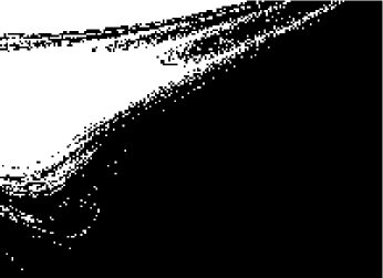
FIG. 4.: A fractal basin boundary scan in $(\dot{r},r\dot{\phi})$ varying over initial values in $0<\dot{r}<0.035$ and $0.425<r\dot{\phi}<0.443125$. All 40,000 orbits have a maximally spinning black hole and a lighter companion with no spin ($\beta=m_{2}/m_{1}=1/3$, $S_{1}=m_{1}^{2}$ and $S_{2}=0$). The initial angle is $\theta_{1}={\rm arccos}({\bf\hat{L}_{N}}\cdot{\bf\hat{S}_{1}})=95{}^{o}$ and initial separation $r/m=5$. $200\times 200$ orbits shown.

FIG. 5.: Top: A three-dimensional plot of an irregular orbit near the basin boundary of fig. 4 with initial velocities $\dot{r}=0.00105$ and $r\dot{\phi}=0.43075$. Bottom: A projection of the orbit onto the $(r,\dot{r})$.

An irregular orbit selected near the fractal boundary is shown the top panel of fig. 5. The bottom panel of fig. 5 is a detail of the projected motion in the $(r,\dot{r})$ plane which shows some threading of the orbit. A full Poincaré section taken as described above confirms that this is not an illusion from the projection. However, the numerical burden is extreme and impractical in nearly all cases of interest. For this reason, we continue to rely on the fractal basin boundaries and only take the projection onto the $(r,\dot{r})$ plane as a crude guide and not as proof of chaos.

In theory, the surface of section technique can also be implemented in the case of two spinning bodies since both are periodic under the precession. In practice this can be difficult since one might have to wait a very long time before ${\bf\vec{S}_{1}}(t)={\bf\vec{S}_{1}}(0)$ at the same time as ${\bf\vec{S}_{2}}(t)={\bf\vec{S}_{2}}(0)$. Alternatively, we can cheat and simply look at the projection of $(r,\dot{r})$ in the full phase space without taking a Poincaré section. This is only used as a crude survey tool. If the projected motion lies on a simple closed curve, the motion is decidedly integrable. If the motion lies on a threaded orbit (such as that of fig. 5), then this indicates the motion might have diffused off of a torus.

Another major shortcoming of the Poincaré surface of section method in this setting is that the 2PN constants of motion are only approximately conserved. Therefore even if one is cautious, the spreading may be a result of the approximation and not a true mark of the destruction of tori. Since this projection is ambiguous, it is only used as a rough guide. For a firm identification of chaos we rely on the unambiguous fractal basin boundaries.

There are other outcomes that could be used to color code a plane in phase space and study the basin boundaries. A set of outcomes based on the number of windings a pair execute would be relevant to the search for gravitational waves. In fig. 6, basin boundaries for the same set of initial conditions are compared. The binaries all have the same initial condition except for the initial angular displacement of the spins. The top panel was originally published in [2]. For that top panel, stable/merger outcomes are used. The initial condition in the $(\theta_{1},\theta_{2})$ plane is color coded white if the pair executes at least 50 orbits and black if the pair merge in under 50 orbits. The lower panel uses a winding criterion: the initial condition in the $(\theta_{1},\theta_{2})$ plane is color coded white if the pair execute more than 50 orbits before merger, black if they merge after executing more than 36 orbits (but less than 50), dark grey if the pair merge having executed 36 orbits, and light grey if the pair merge having executed less than 36 orbits. The mixed basin boundaries show that there is some unpredictability in the number of orbits executed in the conservative system.

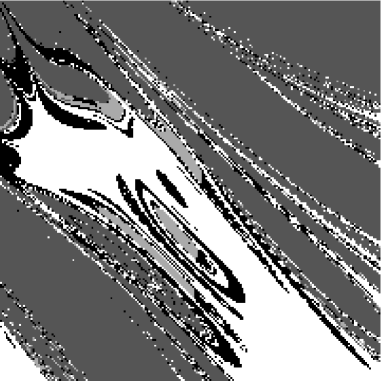
FIG. 6.: All orbits have $m_{2}/m_{1}=1/3$, $r=5m$, and $r\dot{\phi}=0.45$. The initial angles are varied in the $(\theta_{1},\theta_{2})$ plane over the ranges $140.375{}^{o}\leq\theta_{1}\leq 157.5635{}^{o}$ and $45.8367{}^{o}\leq\theta_{2}\leq 63.025411{}^{o}$. Top: Figure from The fractal basin boundaries built up using the stable/merger criteria. Bottom: The fractal basin boundaries built up using a critical winding criterion. A resolution of $200\times 200$ orbits.

We discuss dissipation in §VII. We point out here that when dissipation is included, there is less fractal structure when the critical windings are used as outcomes. This indicates that with dissipation included the number of windings executed by a binary might be predictable. However there is still structure in the basin boundaries when other outcomes are used indicating that not all features of the wave form will evolve predictably.

IV The binary mass ratio

The binary mass ratio $\beta=m_{2}/m_{1}$ primarily effects the cone of precession. The lighter the relative mass of the companion, the larger the band in which the orbital plane will precess and the larger the corresponding modulation of the waveform [13, 14]. The orbital plane will precess around ${\bf\vec{J}}$ with an angle of inclination

$$\cos{i}={\bf\hat{L}_{N}}\cdot{\bf\hat{J}}={{1+(S/L_{N})\cos\theta_{S}}\over\sqrt{1+(S/L_{N})^{2}+2(S/L_{N})\cos\theta_{S}}}$$ (10)

where $\cos\theta_{S}\equiv{\bf\hat{L}_{N}}\cdot{\bf\hat{S}}$ as in fig. 1 and the total angular momentum has been used to lowest order, ${\bf\hat{J}}\sim{\bf\hat{L}_{N}}+{\bf\hat{S}}$. The angle subtended changes as the angle between ${\bf\vec{L}_{N}}$ and ${\bf\vec{S}}$ changes. This leads to the additional tilting back and forth on top of the simple precession. The ratio $S/L_{N}$ can be estimated by taking $L_{N}\sim\mu(mr)^{1/2}$ for a nearly circular orbit. Consider the extremes when the more massive object spins with $S_{1}=m_{1}^{2}$ to get an upper range and the opposite regime when the lighter star spins with $S_{2}=m_{2}^{2}$ to get a lower range:

$$\left(m_{2}\over m_{1}\right)\left(m/r\right)^{1/2}\leq{S\over L_{N}}\leq\left({m_{1}\over m_{2}}\right)\left(m/r\right)^{1/2}\ \ .$$ (11)

For very small $S/L_{N}$, the precession cone angle is so tight that modulations of the gravitational wave signal will not be substantial. Notice from the left-hand side of eqn. (11) that if only the lighter object spins then $S/L_{N}$ is small for all $r$. This may explain why Ref. [1] found chaos for a test particle around a Schwarzschild black hole only if the light companion had a spin $S_{2}>0.64m_{2}m_{1}$ for $m_{1}\gg m_{2}$, which exceeds the maximal spin of $S_{2}=m_{2}^{2}$. The 2PN expansion to the two-body problem allows both black holes to spin and precess. When the more massive object spins maximally, then $S/L_{N}$ is large for $m_{1}\gg m_{2}$. For a $10:1$ mass ratio, $S/L_{N}\sim 1$ for $r\sim 100m$. As a result, for large mass ratios, the orbital plane subtends a larger angle at a given radius and modulation will be correspondingly larger [13, 14]. Consider fig. 2 versus fig. 3. In both figures, the more massive BH spins maximally ($S_{1}=m_{1}^{2}$) with a spin displacement of ${\bf\hat{L}_{N}}\cdot{\bf\hat{S}}=\cos(45^{\circ})=1/\sqrt{2}$. In both figures, the companion has no spin. The difference between the two figures is the mass ratio. In fig. 2, the mass ratio is $\beta=1.4/10$ and the angle subtended at $r=20$ is $i\sim 28^{\circ}$. In fig. 3, the mass ratio is $\beta=1/3$ and the angle subtended at $r=20$ is $i\sim 18^{\circ}$. The band subtended by the precessing plane is larger for the smaller mass ratio, although it is substantial in both cases.

We can invert eqn. (10) using the right-hand-side of eqn. (11) to write the radius at a given inclination,

$$\left({r\over m}\right)^{1/2}\sim\left(m_{1}\over m_{2}\right)\times$$ (12)

$$\left[{\cos^{2}i-\cos^{2}\theta_{1}\over\cos\theta_{1}(1-\cos^{2}i)+\sqrt{\cos^{2}i(1-\cos^{2}i)(1-\cos^{2}\theta_{1})}}\right]$$ (13)

with $\cos\theta_{1}\equiv{\bf\hat{L}_{N}}\cdot{\bf\hat{S}_{1}}$. We could take this as an indicator for the radius at which precession becomes important. Letting $i\sim 15^{\circ}$ and $\theta_{1}\sim 45^{\circ}$, then

$${r\over m}\sim 4\times\left(m_{1}\over m_{2}\right)^{2}.$$ (14)

For circular motion, $L\sim\mu(mr)^{1/2}$ and $m\dot{\phi}\sim\left(m/r\right)^{3/2}$ and the frequency of the emitted wave, $f\sim\dot{\phi}/\pi$ is roughly

$$f\sim 9\times 10^{3}{\beta^{3}}\left(M_{\odot}\over m\right)\ {\rm Hz}.$$ (15)

For a BH/BH binary with $\beta\sim 1/3$ and $m=20M_{\odot}$, then $f\sim{\cal O}(10)$ Hz when the spin precession angle opens to $i\sim 15^{\circ}$ and the effects on the gravitational wave should be noticeable. For a BH/NS binary with $\beta\sim 1.4/10$ and $m=11.4$, then $f\sim{\cal O}({1})$ Hz when the spin precession angle opens to $i\sim 15^{\circ}$. To emphasize, precession will be important for these and larger frequencies as the pairs sweep through the interferometer’s bandwidth.

FIG. 7.: The waveform, Newtonian angular momentum and spin for the orbit of fig. 3. Top: The waveform $h_{+}$. Bottom: three-dimensional view of the precession of ${\bf\vec{S}_{1}}$.

While we can conclude that smaller mass ratio means a wider precessional angle, the dependence of the regularity of the motion on $\beta$ within that band is not yet clear. Within the bulk precession, the orbital plane tilts back and forth, sometimes regularly and sometimes erratically. Orbits can subtend roughly the same cone but some occupy the band more regularly than others. A hint of the effect of $\beta$ on regularity comes from a comparison of frequencies. An instantaneous orbital frequency can be defined roughly as

$$\omega\sim{{L_{N}}\over\mu r^{2}}$$ (16)

for comparison with the instantaneous spin precession frequency of the larger object (neglecting spin-spin coupling just for the crude estimate)

$$\Omega_{1}\sim\left(2+{3m_{2}\over 2m_{1}}\right){L_{N}\over r^{3}}$$ (17)

so that

$${\omega\over\Omega_{1}}\simeq{\left(\beta+1\right)^{2}\over\beta\left(2+{3\beta/2}\right)}\left({r\over m}\right).$$ (18)

Therefore $\omega/\Omega_{1}$ is always large. The pair executes many orbital windings per spin precession. This hints that the chaotic behaviour may be related to modulation diffusion where a slowly varying parameter, in this case ${\bf\vec{S}_{1}}$, facilitates chaotic resonances between coordinates, in this case $\theta$ and $\phi$ [24].

However, compared to the instantaneous precession frequency of the spin of the lighter object

$${\omega\over\Omega_{2}}\simeq{\left(\beta+1\right)^{2}\over\left(2\beta+{3/2}\right)}\left({r\over m}\right).$$ (19)

This ratio is not as large for small $\beta$ so the lighter companion always precesses much more than the heavy black hole. As argued in §V, the spin of the companion encourages irregularity and the fact that $\Omega_{2}/\Omega_{1}<1$ may account for some of this effect.

In general, the mass ratio $\beta=m_{2}/m_{1}$ seems to effect the bulk shape of the precession and gravitational wave modulation. By eqns. (18) and (19), $\beta$ may determine the radii at which chaotic resonances will occur. Still, it is unclear how much the mass ratio impacts the details of the motion.

For comparison with later cases, the waveform emitted by the BH/BH binary of fig. 3 is shown in the top panel of fig. 7. Even though the precession is fairly regular, it does modulate the wave amplitude and frequency. The modulation of the waveform has been minimized by placing the binary directly above the detector. Tail-effects are neglected throughout. A three dimensional view of the precession of the spin ${\bf\vec{S}_{1}}$ is shown in the lower panel of fig. 7.

V Second Spin

The effect of spinning up the lighter companion can be studied by starting with the orbits of fig. 4. Even a small second spin will cause further diffusion in phase space. When the second spin is maximal, the fraying of the projection in $(r,\dot{r})$ increases. Fig. 8 shows an irregular three-dimensional orbit, the projected motion in $(r,\dot{r})$, and the waveform when both objects spin maximally. Fig. 9 shows the precession of both spin vectors.

FIG. 8.: An irregular orbit with $\beta=m_{2}/m_{1}=1/3$, $S_{i}=m_{i}^{2}$. The initial conditions for the orbit are $r/m=6$ and $\dot{r}=0.025$ $r\dot{\phi}=0.365$. Top: three-dimensional view of the orbit. Middle: a projection of the orbit onto the $(r,\dot{r})$ plane. Bottom: the waveform.

The fraying of the orbit in $(r,\dot{r})$ indicates that the motion might not be confined to a torus. As discussed in §III, the projection is a hint of nointegrability; that is, of chaos. However, as already mentioned, the projection alone is not enough to conclude there is chaos. A full basin boundary analysis shows that this orbit occurs near a fractal boundary giving every indication the orbit is chaotic. Notice in fig. 9 that the spin of the lighter star precesses more than the spin of the heavier object as expected from eqns. (18)-(19).

FIG. 9.: The Spins for the orbit of fig. 8. Top: three-dimensional view of the precession of ${\bf\vec{S}_{1}}$. Bottom: three-dimensional view of the precession of ${\bf\vec{S}_{2}}$.

VI Eccentricity

Binary black holes formed in dense stellar regions are thought to have a roughly thermal distribution in eccentricity with a slight enhancement of high $e$ at the time of formation [8]. While many of these may still have time to circularize before merger, it is worth investigating the role of eccentricity on the regularity of the orbit. Large misaligned spins necessarily induce eccentricity. Chaos seems to occur when angular momentum sloshes between spins and the orbit. It is difficult to separate cause and effect. Still, it is obvious that eccentricity alone is not the culprit.

FIG. 10.: A regular but eccentric orbit with $\beta=m_{2}/m_{1}=1/3$, $S_{1}=m_{1}^{2}$ and $S_{2}=0$. The initial angle $\theta_{1}={\rm arccos}({\bf\hat{L}_{N}}\cdot{\bf\hat{S}_{1}})=45{}^{o}$. The initial conditions for the orbit are $r/m=20$ and $r\dot{\phi}=0.2$. Top: three-dimensional view of the orbit. Middle: a projection of the orbit onto the $(r,\dot{r})$ plane. Bottom: the waveform.

Consider fig. 10 where only one of the holes is spinning. The top panel shows the three-dimensional orbit which does have irregular features. However, this is deceptive. It is well known that Keplerian orbits are closed ellipses while relativistic, elliptical orbits precess within the orbital plane. The entire plane then precesses due to the spins. What is being witnessed in the top panel of fig. 10 is this double precession. The middle panel shows complete regularity of the orbit in $(r,\dot{r})$. Motion in this coordinate is confined to a torus. The waveform shown in the bottom panel shows several expected features. Since the orbit is elliptical, the gravitational waves oscillate at once, twice and three times the orbital frequency which changes the spectrum from that for a circular orbit. The double precession then modulates the amplitude and phase on top of these oscillations. Even though this motion is regular (for $S_{2}=0$), in the sense of being predictable, the modulation of the waveform from the double precession must certainly impact observations gained through the method of matched filtering.

Eccentric orbits do show chaotic precession when the companion spins rapidly as well. (Note that when both stars spin, there are no circular orbits [14].)

VII Dissipation

The emission of gravitational waves dissipates energy and angular momentum. The spins are not strongly effected by the loss of gravitational waves which carry away orbital angular momentum and circularize the orbit. The irregularity of a dissipative binary can be evaluated in terms of how many orbits the pair executes as it passes through the successive regions in the conservative system [26]. The most efficient way to do this is again using the fractal basin boundaries. As pointed out in Ref. [26], when dissipation is included the boundaries will never be truly fractal. Like a snowflake, the self-similar structure will cutoff at some physical limit. However, if a color coded basin boundary shows substantial structure, it is fair to say, the participating orbits are influenced by irregularity. The smaller the scale at which the cutoff occurs, the more irregular the history of that set of orbits.

Fig. 11 illustrates the dissipative inspiral of 90,000 maximally spinning black hole pairs with $\beta=1/3$. The orbits all coalesce due to energy lost to gravitational waves. The initial condition in $(\theta_{1},\theta_{2})$ is color coded black if the pair merges from above the $z$-axis and white if the pair merges from below the $z$-axis [2]. The dissipative system does not provide any ideal outcomes, but this criterion should not falsely introduce structure. The top panel of fig. 11 shows some structure for maximal spins while the lower panel of fig. 11 shows substantially less structure for spins $1/10$ of maximal. Incidentally, even more structure is seen for BH/NS binaries with $\beta=1.4/10$ [2].

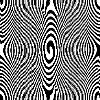
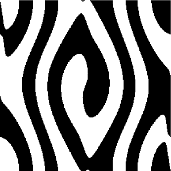
FIG. 11.: Coalescing orbits with radiative reaction for $\beta=1/3$ with $r/m=25$. The slice through phase spans scans over initial orientation of the spins: $-180{}^{o}\leq\theta_{1}\leq 180{}^{o}$ and $-180{}^{o}\leq\theta_{2}\leq 180{}^{o}$. Upper Panel: Spins are maximal $S_{i}=m_{i}^{2}$. Lower Panel: Spins are 10 times smaller, $S_{i}=0.1\ m_{i}^{2}$. $300\times 300$ orbits shown in each panel.

The orbits begin fairly regularly although the precession modulates the waveform. Given unlimited access to theoretical templates, matched filtering could in principle glean a confident signal, at least until the pair drew near the unstable orbits. The orbit becomes more irregular as the separation closes and the pair passes near the underlying conservative trajectory in fig. 8 just before plunge. Since matched filtering relies on the template remaining in phase with the data for many cycles, one might hope that a disruption of the last few cycles would not be serious. Many authors have already argued for the use of other methods at these close separations (see [19] and the references therein). However, others have argued [27] that these last few orbits are heavily weighted and therefore critical for a successful detection. More important than the visually obvious amplitude modulation the precession modulates the gravitational wave frequency. A frequency space analysis is still required to determine if the modulation inhibits detectability of such irregular waves.

VIII Summary

It is reasonable to conclude for a typical stellar mass BH/BH system that if the primary black hole spins rapidly, the orbital plane will precess unpredictably for the final orbits before merger. The dependence of the precessional motion was tested as a function of three parameters:

$\bullet$ $\beta=m_{2}/m_{1}$: As was already known, the smaller the mass ratio, the thicker the band occupied by the precessing orbit [13, 14]. A ratio of $\beta=1/3$ is small enough for precession to modulate observable gravitational waves. The mass ratio may also determine the radius at which chaotic resonances occur by effecting the relative orbital and spin frequencies.

$\bullet$ spin magnitudes: The transition to chaos occurs as the spin magnitudes and misalignments are increased. There can be chaotic motion even if only one body spins. If it is a light companion spinning, then the magnitude of the spin has to be larger than maximal [1]. If it is the heavier object, then chaos can occur for rapid but physically allowed black hole spins. This is true for both BH/BH and BH/NS pairs. For a given eccentricity and radial separation, a transition to chaos can occur as the spin of the companion is increased.

$\bullet$ eccentricity: Large misaligned spins cause eccentricity which may therefore be a feature common to chaotic orbits. However, large eccentricity alone certainly does not cause chaos. If chaos is indeed occurring near the unstable homoclinic orbits of Ref. [10], then we might expect a fair spread in eccentricities for chaotic orbits since the homoclinic orbits occur with a broad range of eccentricities. Importantly, even for a completely regular orbit the usual relativistic precession of an elliptic orbit in the plane becomes superposed on the precession of the orbital plane. This combination, though not an indication of chaos, does lead to a complicated modulation of the gravitational wave signal.

The most pressing question remains, will irregular orbits of coalescing binaries hinder observations? A detailed study of the modulated gravitational wave is needed. A conjecture is that an erratic precession of the orbital plane will result in an erratic frequency or phasing of the gravitational wave but will not alter the total number of cycles much. If this conjecture is fair, observations in the chaotic regime may be salvaged with a modification of the matched filtering method. As direct detections become more acute, we can aspire to watch the transition from regular to irregular motion. We might then witness the signature nonlinearity of general relativity determine the fate of chaotic binaries.

I am grateful to V. Kalogera, V. Kaspi, S. Portegies Zwart and F. Rasio for sharing their expertise. I want to especially thank J.D. Barrow, M. Bucher, E. Bertschinger, E. Copeland, N.J. Cornish, P. Ferreira, L. Grischuk, S.A. Hughes, R. O’Reilly, and B.S. Sathyaprakash for their insightful comments and support. I also want to thank the theoretical physics group at Imperial College for their hospitality. This work is supported by PPARC.

A 2PN Equations of Motion

In the notation of Ref. [14], the center of mass equations of motion in harmonic coordinates are

$$\ddot{{\bf\vec{r}}}={\bf\vec{a}_{PN}}+{\bf\vec{a}_{SO}}+{\bf\vec{a}_{SS}}+{\bf\vec{a}_{RR}}$$ (A1)

with ${\bf\vec{r}}=r{\bf\hat{r}}$. The right hand side is the sum of the contributions to the relative acceleration from the Post-Newtonian (PN) expansion, the spin-orbit (SO) and spin-spin (SS) coupling and from the radiative reaction (RR). The explicit terms are quoted from Ref. [14]. The following notation is used: ${{\bf\vec{v}}}={d{{\bf\vec{r}}}/dt}$, ${{\bf\hat{n}}}\equiv{{{\bf\vec{r}}}/r}$, $\mu\equiv m_{1}m_{2}/m$, $\eta\equiv\mu/m$, $\delta m\equiv m_{1}-m_{2}$, ${{\bf\vec{S}}}\equiv{{\bf\vec{S}_{1}}}+{{\bf\vec{S}_{2}}}$, and ${{\bf\vec{\Delta}}}\equiv m({{\bf\vec{S}_{2}}}/m_{2}-{{\bf\vec{S}_{1}}}/m_{1})$. The ${\bf\vec{a}_{PN}}={\bf\vec{a}_{N}}+{\bf\vec{a}_{1PN}}+{\bf\vec{a}_{2PN}}$ with

$${{\bf\vec{a}_{N}}}=-{m\over r^{2}}{{\bf\hat{n}}},$$ (A2)

$${{\bf\vec{a}_{1PN}}}=-{m\over r^{2}}\left\{{{\bf\hat{n}}}\left[(1+3\eta)v^{2}-2(2+\eta){m\over r}-{3\over 2}\eta\dot{r}^{2}\right]-2(2-\eta)\dot{r}{{\bf\vec{v}}}\right\},$$ (A3)

$${{\bf\vec{a}_{2PN}}}=-{m\over r^{2}}\biggl{\{} {{\bf\hat{n}}}\biggl{[}{3\over 4}(12+29\eta)\left({m\over r}\right)^{2}+\eta(3-4\eta)v^{4}+{15\over 8}\eta(1-3\eta)\dot{r}^{4}$$ (A6)

$$\mbox{}-{3\over 2}\eta(3-4\eta)v^{2}\dot{r}^{2}-{1\over 2}\eta(13-4\eta){m\over r}v^{2}-(2+25\eta+2\eta^{2}){m\over r}\dot{r}^{2}\biggr{]}$$

$$\mbox{}-{1\over 2}\dot{r}{{\bf\vec{v}}}\left[\eta(15+4\eta)v^{2}-(4+41\eta+8\eta^{2}){m\over r}-3\eta(3+2\eta)\dot{r}^{2}\right]\biggr{\}},$$

The radiative reaction term is due to terms to $5/2$PN order and can be expressed as

$${\bf\vec{a}_{RR}}={8\over 5}\eta{m^{2}\over r^{3}}\left\{\dot{r}{{\bf\hat{n}}}\left[18v^{2}+{2\over 3}{m\over r}-25\dot{r}^{2}\right]-{{\bf\vec{v}}}\left[6v^{2}-2{m\over r}-15\dot{r}^{2}\right]\right\},$$ (A7)

The spin-orbit acceleration is

$${\bf\vec{a}_{SO}}={1\over r^{3}}\left\{6{{\bf\hat{n}}}[({{\bf\hat{n}}}\times{{\bf\vec{v}}}){\cdot}(2{{\bf\vec{S}}}+{\delta m\over m}{{\bf\vec{\Delta}}})]-[{{\bf\vec{v}}}\times(7{{\bf\vec{S}}}+3{\delta m\over m}{{\bf\vec{\Delta}}})]+3\dot{r}[{{\bf\hat{n}}}\times(3{{\bf\vec{S}}}+{\delta m\over m}{{\bf\vec{\Delta}}})]\right\}.$$ (A8)

and the spin-spin acceleration is

$${\bf\vec{a}_{SS}}=-{3\over\mu r^{4}}\biggl{\{}{{\bf\hat{n}}}({{\bf\vec{S}_{1}}\cdot{\bf\vec{S}_{2}}})+{{\bf\vec{S}_{1}}}({{\bf\hat{n}}\cdot{\bf\vec{S}_{2}}})+{{\bf\vec{S}_{2}}}({{\bf\hat{n}}\cdot{\bf\vec{S}_{1}}})-5{{\bf\hat{n}}}({{\bf\hat{n}}\cdot{\bf\vec{S}_{1}}})({{\bf\hat{n}}\cdot{\bf\vec{S}_{2}}})\biggr{\}}.$$ (A9)

1 Constants of the Motion

$$E=E_{PN}+E_{SO}+E_{SS},$$ (A10)

where $E_{PN}=E_{N}+E_{1PN}+E_{2PN}$ and

$$E_{N}=\mu\left\{{1\over 2}v^{2}-{m\over r}\right\},$$ (A11)

$$E_{1PN}=\mu\left\{{3\over 8}(1-3\eta)v^{4}+{1\over 2}(3+\eta)v^{2}{m\over r}+{1\over 2}\eta{m\over r}\dot{r}^{2}+{1\over 2}({m\over r})^{2}\right\},$$ (A12)

$$E_{2PN}=\mu\biggl{\{} {5\over 16}(1-7\eta+13\eta^{2})v^{6}-{3\over 8}\eta(1-3\eta){m\over r}\dot{r}^{4}+{1\over 8}(21-23\eta-27\eta^{2}){m\over r}v^{4}$$ (A15)

$$\mbox{}+{1\over 8}(14-55\eta+4\eta^{2})\left({m\over r}\right)^{2}v^{2}+{1\over 4}\eta(1-15\eta){m\over r}v^{2}\dot{r}^{2}-{1\over 4}(2+15\eta)\left({m\over r}\right)^{3}$$

$$\mbox{}+{1\over 8}(4+69\eta+12\eta^{2})\left({m\over r}\right)^{2}\dot{r}^{2}\biggr{\}},$$

$$E_{SO}={1\over r^{3}}{{\bf\vec{L}_{N}}\cdot}({{\bf\vec{S}}}+{\delta m\over m}{{\bf\vec{\Delta}}}),$$ (A16)

$$E_{SS}={1\over r^{3}}\left\{3\left({{\bf\hat{n}}\cdot{\bf\vec{S}_{1}}}\right)\left({{\bf\hat{n}}\cdot{\bf\vec{S}_{2}}}\right)-\left({{\bf\vec{S}_{1}}\cdot{\bf\vec{S}_{2}}}\right)\right\}.$$ (A17)

The total angular momentum is given by

$${{\bf\vec{J}}}={{\bf\vec{L}}}+{{\bf\vec{S}}},$$ (A18)

where

$${{\bf\vec{L}}}={\bf\vec{L}_{PN}}+{\bf\vec{L}_{SO}}$$ (A19)

with ${\bf\vec{L}_{PN}}={\bf\vec{L}_{N}}+{\bf\vec{L}_{1PN}}+{\bf\vec{L}_{2PN}}$ and

$${{\bf\vec{L}_{N}}}\equiv\mu({{\bf\vec{r}}\times{\bf\vec{v}}}),$$ (A20)

$${\bf\vec{L}_{1PN}}={{\bf\vec{L}_{N}}}\left\{{1\over 2}v^{2}(1-3\eta)+(3+\eta){m\over r}\right\},$$ (A21)

$${\bf\vec{L}_{2PN}}={{\bf\vec{L}_{N}}}\biggl{\{} {3\over 8}(1-7\eta+13\eta^{2})v^{4}-{1\over 2}\eta(2+5\eta){m\over r}\dot{r}^{2}$$ (A24)

$$\mbox{}+{1\over 2}(7-10\eta-9\eta^{2}){m\over r}v^{2}$$

$$\mbox{}+{1\over 4}(14-41\eta+4\eta^{2})\left({m\over r}\right)^{2}\biggr{\}},$$

and

$${\bf\vec{L}_{SO}}={\mu\over m}\Biggl{\{} {m\over r}{{\bf\hat{n}}\times}\left[{{\bf\hat{n}}\times}\left(3{{\bf\vec{S}}}+{\delta m\over m}{{\bf\vec{\Delta}}}\right)\right]$$ (A26)

$$\mbox{}-{1\over 2}{{\bf\vec{v}}\times}\left[{{\bf\vec{v}}\times}\left({{\bf\vec{S}}}+{\delta m\over m}{{\bf\vec{\Delta}}}\right)\right]\Biggr{\}}.$$

REFERENCES

- [1] S.Suzuki and K.Maeda, Phys. Rev. D. 55 4848 (1997).
- [2] J. Levin, Phys. Rev. Lett. 84 3515 (2000).
- [3] G. Contopolous, Proc. R. Soc. A431 183 (1990); Proc. R. Soc. A435 551 (1990).
- [4] L.Bombelli and E.Calzetta, Class. Quantum. Grav. 9 2573 (1992).
- [5] C. P. Dettmann, N. E. Frankel and N. J. Cornish, Phys. Rev. D50, R618 (1994); Fractals, 3, 161 (1995).
- [6] N.J. Cornish and N.E.Frankel, Phys. Rev. D 56 1903 (1997).
- [7] J.Levin, Phys. Rev. D. 60 64015 (1999).
- [8] S.F.Portegies-Zwart and S.L. McMillan, astro-ph/9910061; astro-ph/9912022.
- [9] A. I. MacFadyen and S.E. Woosley, Astrophys. J. 524 (1999) 262; A. I. MacFadyen, S.E. Woosley and A. Heger, Astrophys. J. 550 (2001) 410.
- [10] J. Levin, R. O’Reilly, and E.J. Copeland, Phys. Rev. D 62 (2000) 024023.
- [11] V.Kalogera, astro-ph/9911417.
- [12] For reviews on gravitational wave astronomy see K.S.Thorne, gr-qc/9704042; B.F. Schutz, Class. Quant. Grav. 16 A131 (1999). L.P. Grishchuk, V.M. Lipunov, K.A. Postnov, M.E. Prokhorov and B.S. Sathyaprakash astro-ph/0008481.
- [13] T.A. Apostolatos, C. Cutler, G.J. Sussman, and K.S. Thorne, Phys. Rev. D 15 6274 (1994).
- [14] L. Kidder, Phys. Rev. D. 52 821 (1995).
- [15] L. Blanchet and T. Damour, Ann. Inst. Henri Poincaré A, 50 377 (1989); T. Damour and B.R. Iyer, Ann. Inst. Henri Poincaré 54 115 (1991).
- [16] L.E.Kidder, C.M.Will and A.G.Wiseman, Phys. Rev. D 47 3281 (1993).
- [17] T. Damour, Phys. Rev. D 64 (2001) 124013.
- [18] L.S. Finn and D.F. Chernoff, Phys. Rev. D. 47 2198 (1993).
- [19] S. A. Hughes, comment to appear in Phys. Rev. Lett..
- [20] N.J. Cornish, Proceedings of the Eigth Marcel Grossmann Meeting, Jerusalem, June 1992 gr-qc/9709036; also see gr-qc/9602054.
- [21] N.J. Cornish and J.J. Levin, Phys. Rev. Lett. 78 998 (1997); Phys. Rev. D.55 7489 (1997).
- [22] T. Damour and N. Deruelle, C.R. Acad. Sci. Paris 293 537 (1981); 293 877 (1981); L.P. Grishchuk and S.M. Kopejkin, contribution to Relativity in Celestial Mechanics and Astrometry, ed J. Kovalevsky and V.A. Brumberg (Reidel, Dordrecht, 1986), p. 19.
- [23] L.E. Kidder, C.M.Will, and A.G. Wiseman, Phys. Rev. D 47 4183 (1993).
- [24] A. J. Lichtenberg & M. A. Lieberman, Regular and chaotic dynamics, (Springer-Verlag, New York, 1992).
- [25] E. Ott, Chaos in dynamical systems, (Cambridge University Press, Cambridge, 1993).
- [26] see also the comment by N.J. Cornish to be published in Phys. Rev. Lett..
- [27] R.P. Croce, Th. Demma, V. Pierro, I.M. Pinto, D. Churches, and B.S. Sathyaprakash, gr-qc/0008059.