On the contribution of density perturbations and gravitational waves to the lower order multipoles of the Cosmic Microwave Background Radiation

Abstract

The important studies of Peebles, and Bond and Efstathiou have led to the formula $C_{\ell}=const/[\ell(\ell+1)]$ aimed at describing the lower order multipoles of the CMBR temperature variations caused by density perturbations with the flat spectrum. Clearly, this formula requires amendments, as it predicts an infinitely large monopole $C_{0}$, and a dipole moment $C_{1}$ only $6/2$ times larger than the quadrupole $C_{2}$, both predictions in conflict with observations. We restore the terms omitted in the course of the derivation of this formula, and arrive at a new expression. According to the corrected formula, the monopole moment is finite and small, while the dipole moment is sensitive to short-wavelength perturbations, and numerically much larger than the quadrupole, as one would expect on physical grounds. At the same time, the function $\ell(\ell+1)C_{\ell}$ deviates from a horizontal line and grows with $\ell$, for $\ell\geq 2$. We show that the inclusion of the modulating (transfer) function terminates the growth and forms the first peak, recently observed. We fit the theoretical curves to the position and height of the first peak, as well as to the observed dipole, varying three parameters: red-shift at decoupling, red-shift at matter-radiation equality, and slope of the primordial spectrum. It appears that there is always a deficit, as compared with the COBE observations, at small multipoles, $\ell\sim 10$. We demonstrate that a reasonable and theoretically expected amount of gravitational waves bridges this gap at small multipoles, leaving the other fits as good as before. We show that the observationally acceptable models permit somewhat ‘blue’ primordial spectra. This allows one to avoid the infra-red divergence of cosmological perturbations, which is otherwise present.

1 Introduction

The important studies of Peebles [1982, 1993] and Bond and Efstathiou [1987, 1990] have led to the formula for the multipole moments of the CMB radiation, $C_{\ell}$, caused by small density perturbations with flat spectrum (also known as Harrison–Zel’dovich–Peebles, or scale-invariant spectrum; spectral index ${\mathrm{n}}=1$):

$$C_{\ell}=\frac{const}{\ell(\ell+1)}.$$ (1)

This formula aims to describe the lower order multipoles of the CMBR variations in a spatially flat universe. The general acceptance of this result is reflected in the fact that the $C_{\ell}$ distributions are usually plotted in terms of the function $\ell(\ell+1)C_{\ell}$ versus $\ell$. In these units, formula (1) is conveniently plotted as a horizontal line.

Clearly, formula (1) was derived under some assumptions, and this derivation requires amendments. Indeed, let us start from the monopole moment $C_{0}$, setting $\ell=0$ in this formula. Expression (1) predicts infinity for $C_{0}$, in conflict with observations. Surely, it would be difficult to observationally distinguish a monopole component caused by perturbations from the isotropic unperturbed temperature $T_{0}$, but it is strange that a theoretical formula gives infinity for an effect produced by small perturbations. Let us now consider the dipole, $\ell=1$, and the quadrupole, $\ell=2$, moments. According to (1), the quantities $C_{1}$ and $C_{2}$ are numerically of the same order of magnitude, $C_{1}=(6/2)C_{2}$. However, we know from observations that the observed dipole variation of the temperature is about 100 times larger than the observed quadrupole variation.

The predictions of formula (1) also seem to disagree with independent theoretical studies. According to Grishchuk & Zel’dovich [1978], in the limit of long-wavelength perturbations, which normally provide dominant contributions to the $\ell=0$ and $\ell=2$ multipoles, the monopole and quadrupole variations of the CMBR temperature should be small and approximately equal. At the same time, the dipole variation should be suppressed, as compared with the monopole and quadrupole, in proportion to the ratio $l_{{\mathrm{H}}}/\lambda$, where $l_{{\mathrm{H}}}$ is the Hubble radius and $\lambda$ is the perturbation’s wavelength, $\lambda\gg l_{{\mathrm{H}}}$. The multipole moments $C_{\ell}$, being quadratic in the temperature variations, contain this factor in the second power. The factor $l_{{\mathrm{H}}}/\lambda$ becomes much larger than 1 in the opposite limit of short-wavelength perturbations, $\lambda\ll l_{{\mathrm{H}}}$. The dipole component is, thus, expected to be very sensitive to short waves, and its value should eventually exceed the values of the monopole and quadrupole components, as soon as the contribution of short-wavelength perturbations is also included. However, formula (1) suggests results differing from these conclusions. The discrepancy is especially troublesome, as the derivation of (1) seems to have taken into account the perturbations of all wavelengths. Indeed, this formula arises from the table integral (discussed below in Section 4)

$$\int_{0}^{\infty}[j_{\ell}(n\xi)]^{2}\frac{{\mathrm{d}}n}{n}=\frac{1}{2\ell(\ell+1)},$$

where the integration over wave-numbers $n$ ranges formally from zero to infinity. Therefore, according to this integral, the very short-wavelength perturbations have also been taken into account in the calculation of all $C_{\ell}$’s, including the dipole $C_{1}$.

The demonstrated deficiencies of formula (1) for $\ell=0$ and $\ell=1$ indicate that there could also be significant deviations from the values suggested by (1) in the case of $\ell=2$ and higher order multipoles. This consideration has prompted us to reanalyse the derivation of formula (1). In Section 2 we introduce the necessary notations and remind the reader the basics of the Sachs–Wolfe result [1967]. For the purpose of later comparison with observations, we consider primordial spectra with arbitrary spectral indices, so that the flat spectrum ${\mathrm{n}}=1$ is simply a particular case. Section 3 summarises the statistical assumptions and defines the multipole moments. In Section 4 we identify the terms that were dropped out in the course of the original derivation of formula (1). We show the importance of these terms and restore them. After this correction, the numerical values of the monopole and quadrupole moments become comparable to each other, while the dipole moment becomes sensitive to short-wavelength perturbations, as it should. At the same time, the correct formula for $C_{\ell}$ requires the function $\ell(\ell+1)C_{\ell}$ to deviate from the horizontal line and grow with $\ell$ for $\ell\geq 2$. Formally, this growth would be unlimited if one were allowed to use the primordial power-law spectrum for arbitrarily large values of the wavenumber $n$. However, it is known that the primordial power spectrum of density perturbations should experience a turnover, caused by the transition of the cosmological expansion from the radiation-dominated to the matter-dominated regime [1983, 1993]. By the time of decoupling, the primordial spectrum gets modified. Mathematically, the original power spectrum gets multiplied by the modulating function (transfer function). The modulating function is practically unity in the spectral region of long-wavelength perturbations, but it strongly suppresses the power in short-wavelength perturbations. As a result, the growth of the function $\ell(\ell+1)C_{\ell}$ terminates and is being followed by its decline at multipoles, roughly, around $\ell=200$. This causes the function $\ell(\ell+1)C_{\ell}$ to form the first peak, recently observed [2000, 2000, 2000]. The following (less prominent) peaks of the modulating function are responsible for the further peaks of the function $\ell(\ell+1)C_{\ell}$. In Section 5 we analyse in detail the form of the modulating function and derive the possible (theoretical) positions and heights of the first peak. We think that the origin of the subsequent peaks in the $\ell$-space is due to the modulation of the metric power spectrum of density perturbations (oscillations in the $n$-space). This modulation, in its turn, entirely arises due to the standing-wave character of the initial density perturbations. Travelling sound waves in the radiation-dominated era would not have produced Sakharov oscillations at the time of decoupling, as was explained long ago (see Section 11.6 in Zel’dovich & Novikov [1983]). The recent paper [2001] may be providing support to this interpretation of the peaks. However, the origin and position of secondary peaks is not the subject of this paper, so we leave the door open for alternative interpretations. The full computation of all multipoles is presented in Section 6. We replace the existing uncertainties about the matter content of the Universe by the two phenomenological parameters: the decoupling red-shift $z_{{\mathrm{dec}}}$ and the matter-radiation equality red-shift $z_{{\mathrm{eq}}}$. We also vary the third parameter, $\beta$, which characterises the spectral slope of the primordial perturbations. (The flat spectrum ${\mathrm{n}}=1$ corresponds to $\beta=-2$.) We show how the distributions of multipole moments depend on the choice of these parameters. Since we concentrate on anisotropies of gravitational origin, the chemical composition of matter in the Universe is unimportant, as long as the perturbations can be described by solutions to the perturbed Einstein equations at the radiation-dominated stage (equation of state $p=\epsilon/3$) followed by the matter-dominated stage (equation of state $p=0$). Section 7 gives a preliminary comparison of the calculated multipole moments (including the dipole) with the available CMBR observations. We require the theoretical (statistical) dipole, as well as the location and the height of the first peak, to be as close as possible to their observed values. It appears, then, that the values of the COBE-observed [1992] multipoles, around $\ell=10$, are somewhat larger than the theoretical curves for $\ell(\ell+1)C_{\ell}$ would require. The, so far neglected, intrinsic anisotropies (temperature variations at the last scattering surface) can only increase the height of the first peak making this discrepancy larger. The most natural way of removing this discrepancy is to take into account gravitational waves. They mostly contribute to the multipoles from $\ell=2$ to approximately $\ell=30$, without changing the dipole, and not seriously affecting the location and height of the peak. Section 8 describes the contribution of gravitational waves. In effect, we calculate the amount of gravitational waves needed in order to raise the ‘plateau’ at lower $\ell$’s to the actually observed level. In Section 9 we again compare the theory with observations, this time including gravitational waves, and discuss the values of the parameters $z_{{\mathrm{dec}}}$, $z_{{\mathrm{eq}}}$, $\beta$ that produce distributions $\ell(\ell+1)C_{\ell}$ in better agreement with CMBR observations. We argue that a slightly larger amount of gravitational waves allows the primordial spectrum to be somewhat ‘blue’ (${\mathrm{n}}>1$ or $\beta>-2$) instead of being flat. The $C_{\ell}$’s produced by such ‘blue’ spectra are still consistent with the discussed observations. We consider this fact as a satisfactory conclusion, since, from the theoretical standpoint, the flat spectrum and ‘red’ spectra (${\mathrm{n}}<1$ or $\beta<-2$) are undesirable. Indeed, the mean square values of the metric (gravitational field) fluctuations are logarithmically divergent for the ${\mathrm{n}}=1$ case and power-law divergent for all ${\mathrm{n}}<1$, in the limit of long waves. The removal of these divergences would require extra assumptions. Appendix A contains some technical details of the derivation of the corrected formula for $C_{\ell}$.

2 The Sachs-Wolfe result and growing density perturbations

Following Landau & Lifshitz [1975], Sachs & Wolfe [1967], we describe a FLRW universe and the perturbed gravitational field by the line element

$${\mathrm{d}}s^{2}=a^{2}[{\mathrm{d}}\eta^{2}-(\delta_{ij}+h_{ij}){\mathrm{d}}x^{i}\ {\mathrm{d}}x^{j}],$$

where $h_{ij}$ refers to density perturbations or gravitational waves. In the matter-dominated era (equation of state $p=0$) the scale factor behaves as $a(\eta)\propto\eta^{2}$, which we write as

$$a_{{\mathrm{m}}}\!(\eta)=2l_{{\mathrm{H}}}\ (\eta-\eta_{{\mathrm{m}}})^{2},$$

where $l_{{\mathrm{H}}}$ is the Hubble radius at the present time $\eta=\eta_{{\mathrm{R}}}$. The constant $\eta_{{\mathrm{m}}}$ is needed for further considerations. It is convenient to choose $\eta_{{\mathrm{R}}}-\eta_{{\mathrm{m}}}=1$. With this convention, the wave-length equal to the Hubble radius today corresponds to the wave-number $n_{{\mathrm{H}}}=4\pi$. In the matter-dominated era, the employed coordinate system is both synchronous and comoving - the most convenient choice [1975, 1967]. The elements of plasma emitting the CMB photons, as well as the observer, are ‘frozen’ in the perturbed deforming matter and, by the definition of the comoving coordinate system, have zero velocities with respect to the matter fluid.

Let the direction of observation of a photon emitted at $\eta=\eta_{{\mathrm{E}}}$ be characterised by a unit vector

$${\mathbf{e}}=(\sin\!\theta\ \cos\!\phi,\ \ \sin\!\theta\ \sin\!\phi,\ \ \cos\!\theta).$$ (2)

The relative temperature variation $\delta T/T$ seen in a given direction $(\theta,\phi)$ is described by the integral [1967]

$$\frac{\delta T}{T}\!({\mathbf{e}})=\frac{1}{2}\int_{0}^{\xi}\left.\frac{\partial h_{ij}}{\partial\eta}e^{i}e^{j}\right|_{{\mathbf{x}}={\mathbf{e}}w}{\mathrm{d}}w,$$ (3)

where $\xi=\eta_{{\mathrm{R}}}-\eta_{{\mathrm{E}}}$ and the integration is performed along the path $\eta=\eta_{R}-w$, ${\mathbf{x}}={\mathbf{e}}w$. The quantity $\xi$ is related to the red-shift $z_{{\mathrm{dec}}}$ at decoupling as

$$\xi=1-(1+z_{{\mathrm{dec}}})^{-1/2}.$$ (4)

Typically, the quantity $\xi$ is very close to 1. The fact that the photons coming from different directions might have been emitted at slightly different $\eta_{{\mathrm{E}}}$’s is irrelevant for this calculation, as the integrand in expression (3) is already a small quantity of first order. A first order variation of the upper limit of integration will change the result only in second order of smallness. However, a small initial variation of the temperature over the last scattering surface will be reflected in an additive term to the integral (3). This term would be effective even in the absence of the intervening gravitational field $h_{ij}$ along the photon’s path, and it can be called the intrinsic anisotropy $(\delta T/T)_{{\mathrm{in}}}$. We discuss this term later, in Section 6. As long as further scattering and absorption of CMB photons can be neglected, the integral (3) plus the $(\theta,\phi)$-dependent initial condition $(\delta T/T)_{{\mathrm{in}}}$ fully describe the temperature variations at the point of reception.

We now consider density perturbations. By the time of decoupling, one can normally neglect one of the two linearly-independent solutions to the perturbed equations, and work with the so-called growing solution. In the case of density perturbations at the matter-dominated stage, the growing solution is

$$h_{ij}\!(\eta,{\mathbf{x}})=B\!({\mathbf{x}})\delta_{ij}+\frac{(\eta-\eta_{{\mathrm{m}}})^{2}}{10}B\!({\mathbf{x}})_{,ij}.$$ (5)

Using formula (5) in the integral (3), one obtains [1967]

$$\frac{\delta T}{T}\!({\mathbf{e}})=\frac{1}{10}\left.B_{,f}e^{f}\right|_{{\mathrm{R}}}-\frac{1}{10}(1-\xi)\left.B_{,f}e^{f}\right|_{{\mathrm{E}}}+\frac{1}{10}B|_{{\mathrm{R}}}-\frac{1}{10}B|_{{\mathrm{E}}}.$$ (6)

The exceptional property of the solution (5) is that the integrand becomes a total derivative, so the integral (3) reduces to the values of the under-integral quantity at the end-points of integration. This property is responsible for formula (6). In the general case, this is not true, and is only approximately true for other types of perturbations when they are taken in the long-wavelength limit [1978]. In view of the already existing disorder in the literature with respect to the naming and interpretation of different parts of the Sachs–Wolfe work, we simply call the terms in (6), in order of their appearance, as term I, term II, term III, and term IV. Term I is purely dipolar in its angular structure. Term II consists of all spherical harmonics, including the monopole. Term III has no angular dependence: it only contributes to the monopole. Term IV consists of all spherical harmonics, including the monopole.

One normally assumes that cosmological perturbations can be decomposed over spatial Fourier components with arbitrary wave-vectors ${\mathbf{n}}$. In our case, this amounts to the decomposition of $B({\mathbf{x}})$ as

$$B\!({\mathbf{x}})\equiv\frac{1}{(2\pi)^{3/2}}\int_{-\infty}^{+\infty}{\mathrm{d}}^{3}{\mathbf{n}}\ \left(B_{{\mathbf{n}}}\ {\mathrm{e}}^{{\mathrm{i}}{\mathbf{n\cdot x}}}+B^{\ast}_{{\mathbf{n}}}\ {\mathrm{e}}^{-{\mathrm{i}}{\mathbf{n\cdot x}}}\right).$$ (7)

Since $B\!({\mathbf{x}})$ is a real function, we have included a complex conjugate part to make the expression manifestly real. Using the notation

$$G\!({\mathbf{e}})\equiv\frac{1}{(2\pi)^{3/2}}\ \int_{-\infty}^{+\infty}{\mathrm{d}}^{3}{\mathbf{n}}\ B_{{\mathbf{n}}}\ \left\{{\mathrm{i}}{\mathbf{n\cdot e}}\left[1-(1-\xi){\mathrm{e}}^{{\mathrm{i}}{\mathbf{n\cdot e}}\xi}\right]+\left(1-{\mathrm{e}}^{{\mathrm{i}}{\mathbf{n\cdot e}}\xi}\right)\right\},$$

the temperature variation (6) can be written as

$$\frac{\delta T}{T}\!({\mathbf{e}})=\frac{1}{10}[G\!({\mathbf{e}})+G^{\ast}\!({\mathbf{e}})].$$ (8)

One can expand $G\!({\mathbf{e}})$ over complex spherical harmonics:

$$G\!({\mathbf{e}})=\sum_{\ell=0}^{\infty}\sum_{m=-\ell}^{\ell}g_{\ell m}Y_{\ell m}\!(\theta,\phi).$$ (9)

To do this explicitly, it is convenient to write the wave vector ${\mathbf{n}}$ in the form

$${\mathbf{n}}=(n\sin\!\Theta\ \cos\!\Phi,\ \ n\sin\!\Theta\ \sin\!\Phi,\ \ n\cos\!\Theta)$$ (10)

and use the expansion (see, for example, formula (16.127) of Jackson [1975]):

$$\exp\{{\mathrm{i}}{\mathbf{n\cdot x}}\}=4\pi\ \sum_{\ell=0}^{\infty}\sum_{m=-\ell}^{\ell}{\mathrm{i}}^{\ell}\ j_{\ell}\!(nx)\ Y_{\ell m}^{\ast}\!(\Theta,\Phi)\ Y_{\ell m}\!(\theta,\phi).$$ (11)

As a result, one finds that

term I

produces a purely dipolar variation

$${\mathrm{i}}{\mathbf{n\cdot e}}={\mathrm{i}}\ \frac{4\pi}{3}\ n\sum_{f=-1}^{1}Y_{1f}^{\ast}(\Theta,\Phi)\ Y_{1f}\!(\theta,\phi)=4\pi\ \sum_{\ell=0}^{\infty}\sum_{m=-\ell}^{\ell}{\mathrm{i}}^{\ell}\ \frac{1}{3}n\ \delta_{\ell 1}\ Y^{\ast}_{\ell m}\!(\Theta,\Phi)\ Y_{\ell m}\!(\theta,\phi),$$

term II

contains all spherical harmonics

$${\mathrm{i}}{\mathbf{n\cdot e}}\ (1-\xi)\ {\mathrm{e}}^{{\mathrm{i}}{\mathbf{n\cdot e}}\xi}=4\pi\ \sum_{\ell=0}^{\infty}\sum_{m=-\ell}^{\ell}\sum_{f=-1}^{1}\ {\mathrm{i}}^{\ell+1}\ \frac{4\pi}{3}n(1-\xi)\ j_{\ell}(n\xi)\ Y^{\ast}_{1f}(\Theta,\Phi)\ Y^{\ast}_{\ell m}\!(\Theta,\Phi)\ Y_{1f}(\theta,\phi)\ Y_{\ell m}\!(\theta,\phi),$$

term III

is a purely monopolar contribution

$$1=4\pi\ Y_{00}\!(\theta,\phi)\ Y^{\ast}_{00}\!(\Theta,\Phi)=4\pi\ \sum_{\ell=0}^{\infty}\sum_{m=-\ell}^{\ell}\ {\mathrm{i}}^{\ell}\ \delta_{\ell 0}\ Y^{\ast}_{\ell m}\!(\Theta,\Phi)\ Y_{\ell m}\!(\theta,\phi),$$

term IV

contains all spherical harmonics

$$\exp\{{\mathrm{i}}{\mathbf{n\cdot e}}\xi\}=4\pi\ \sum_{\ell=0}^{\infty}\sum_{m=-\ell}^{\ell}\ {\mathrm{i}}^{\ell}\ j_{\ell}(n\xi)\ Y_{\ell m}^{\ast}\!(\Theta,\Phi)\ Y_{\ell m}\!(\theta,\phi).$$

The part of $g_{\ell m}$ produced by the sum of terms I, III and IV is easy to calculate:

$$\stackrel{{\scriptstyle(1)}}{{g}}\!\!\!\!_{\ell m}=\frac{4\pi}{(2\pi)^{3/2}}\ {\mathrm{i}}^{\ell}\ \int_{-\infty}^{+\infty}{\mathrm{d}}^{3}{\mathbf{n}}\ B_{{\mathbf{n}}}\ \left[\frac{1}{3}n\delta_{\ell 1}+\delta_{\ell 0}-j_{\ell}\!(n\xi)\right]\ Y_{\ell m}^{\ast}\!(\Theta,\Phi).$$

The part of $g_{\ell m}$ contributed by term II demands a more tedious calculation, which results in

$$\stackrel{{\scriptstyle(2)}}{{g}}\!\!\!\!_{\ell m}=\frac{4\pi}{(2\pi)^{3/2}}\ {\mathrm{i}}^{\ell}\ \int_{-\infty}^{+\infty}{\mathrm{d}}^{3}{\mathbf{n}}\ B_{{\mathbf{n}}}\ n(1-\xi)\ \frac{1}{2\ell+1}[(\ell+1)\ j_{\ell+1}\!(n\xi)-\ell\ j_{\ell-1}\!(n\xi)]\ Y_{\ell m}^{\ast}\!(\Theta,\Phi).$$

An outline of the calculation may be found in Appendix A. The total expression $g_{\ell m}=\stackrel{{\scriptstyle(1)}}{{g}}\!\!\!\!_{\ell m}+\stackrel{{\scriptstyle(2)}}{{g}}\!\!\!\!_{\ell m}$ is

$$g_{\ell m}=\frac{4\pi}{(2\pi)^{3/2}}\ {\mathrm{i}}^{\ell}\ \int_{-\infty}^{+\infty}{\mathrm{d}}^{3}{\mathbf{n}}\ B_{{\mathbf{n}}}\ D_{\ell}(n)\ Y_{\ell m}^{\ast}\!(\Theta,\Phi),$$ (12)

where $D_{\ell}(n)$ denotes the combination

$$D_{\ell}(n)\equiv\frac{1}{3}n\ \delta_{\ell 1}+n(1-\xi)\ \frac{1}{2\ell+1}[(\ell+1)\ j_{\ell+1}\!(n\xi)-\ell\ j_{\ell-1}\!(n\xi)]+\delta_{\ell 0}-j_{\ell}(n\xi).$$ (13)

The terms in $D_{\ell}(n)$ shall be referred to as term A, term B, term C and term D, in the order of their appearance in (13). They originate from the terms I - IV introduced earlier, respectively. For the three cases $\ell=0$, $\ell=1$ and $\ell\geq 2$, $D_{\ell}(n)$ is explicitly given by:

$$D_{0}\!(n) = n(1-\xi)\ j_{1}\!(n\xi)+1-j_{0}\!(n\xi),$$

$$D_{1}\!(n) = \frac{1}{3}n+n(1-\xi)\ \frac{1}{3}[2j_{2}\!(n\xi)-j_{0}\!(n\xi)]-j_{1}\!(n\xi),$$ (14)

$$D_{\ell\geq 2}\!(n) = n(1-\xi)\ \frac{1}{2\ell+1}[(\ell+1)\ j_{\ell+1}\!(n\xi)-\ell\ j_{\ell-1}\!(n\xi)]-j_{\ell}(n\xi).$$

Finally, we can write

$$\frac{\delta T}{T}\!({\mathbf{e}})=\frac{1}{10}\ \sum_{\ell=0}^{\infty}\sum_{m=-\ell}^{\ell}[g_{\ell m}\ Y_{\ell m}\!(\theta,\phi)+g_{\ell m}^{\ast}\ Y_{\ell m}^{\ast}\!(\theta,\phi)]$$ (15)

where the $g_{\ell m}$ are given by (12).

The calculation of the integral (3) requires only the knowledge of the gravitational field perturbations $h_{ij}$. However, for further references, we remind the expression for the growing density contrast $(\delta\rho/\rho)\!({\mathbf{x}},\eta)$ associated with the solution (5):

$$\frac{\delta\rho}{\rho}\!({\mathbf{x}},\eta)=-\frac{1}{20}\ (\eta-\eta_{{\mathrm{m}}})^{2}\ \nabla^{2}\ B({\mathbf{x}}).$$

The density contrast is a product of a purely $\eta$-dependent part $(\eta-\eta_{{\mathrm{m}}})^{2}$ and a purely spatial part

$$\frac{\delta\rho}{\rho}\!({\mathbf{x}})\equiv-\frac{1}{20}\nabla^{2}\ B({\mathbf{x}}).$$ (16)

Equation (16) and the decomposition

$$\frac{\delta\rho}{\rho}\!({\mathbf{x}})=(2\pi)^{-3/2}\int_{-\infty}^{+\infty}{\mathrm{d}}^{3}{\mathbf{n}}\left[\left(\frac{\delta\rho}{\rho}\right)_{{\mathbf{n}}}\ {\mathrm{e}}^{{\mathrm{i}}{\mathbf{n\cdot x}}}+\left(\frac{\delta\rho}{\rho}\right)^{\ast}_{{\mathbf{n}}}\ {\mathrm{e}}^{-{\mathrm{i}}{\mathbf{n\cdot x}}}\right]$$ (17)

establish the link between the Fourier components of the density variation and the gravitational field perturbation:

$$\left(\frac{\delta\rho}{\rho}\right)_{{\mathbf{n}}}=\frac{1}{20}n^{2}\cdot B_{{\mathbf{n}}}.$$ (18)

3 Statistical assumptions and multipole moments

Formulae (6), (8) give a temperature variation over the sky, which is produced by a single and deterministic, even if very complicated, perturbed configuration of matter density and gravitational field. We believe, however, that primordial cosmological perturbations may have had a quantum-mechanical origin. To this end, the quantities $h_{ij}$ and $\delta T/T$ are quantum-mechanical operators, and the extraction of the observable information should proceed through the calculation of quantum-mechanical expectation values. Later on, we shall go into some details of the quantum-mechanical generation of cosmological perturbations. However, in this Section, we want to keep the discussion at a phenomenological and as simple as possible level.

We make a simplifying assumption that the quantities $B_{{\mathbf{n}}}$ are classical random functions. Since $B_{{\mathbf{n}}}$ appears in the expression of $\delta T/T$, the temperature variation is also a random function. The angular brackets $<...>$ will denote the ensemble average. A single statistical hypothesis that we shall need in the subsequent calculations is expressed by the equalities $\langle B_{{\mathbf{n}}}\rangle=0$ and

$$\langle B_{{\mathbf{n}}}\ B^{\ast}_{{\mathbf{p}}}\rangle=|B_{n}|^{2}\ \delta^{3}\!({\mathbf{n}}-{\mathbf{p}})=\langle B_{{\mathbf{p}}}\ B^{\ast}_{{\mathbf{n}}}\rangle,\ \ \ \ \ \ \langle B_{{\mathbf{n}}}\ B_{{\mathbf{p}}}\rangle=0=\langle B^{\ast}_{{\mathbf{n}}}\ B^{\ast}_{{\mathbf{p}}}\rangle.$$ (19)

The quantity $|B_{n}|^{2}$ characterises the power spectrum of $B\!({\mathbf{x}})$. Indeed, by multiplying (7) with itself and using (19), one finds

$$\langle B\!({\mathbf{x}})\ B\!({\mathbf{x}})\rangle=\pi^{-2}\ \int_{0}^{\infty}\frac{{\mathrm{d}}n}{n}\ n^{3}\ |B_{n}|^{2}.$$ (20)

The quantity we need to calculate is the correlation function

$$\left\langle\frac{\delta T}{T}\!({\mathbf{e_{1}}})\ \frac{\delta T}{T}\!({\mathbf{e_{2}}})\right\rangle.$$

The vectors ${\mathbf{e_{1}}},\ {\mathbf{e_{2}}}$ refer to two different directions of observation, separated by the angle $\gamma_{12}$. Using the product of two expressions (15), one finds

$$\langle\frac{\delta T}{T}({\mathbf{e_{1}}})\ \frac{\delta T}{T}({\mathbf{e_{2}}})\rangle = \frac{1}{100}\sum_{\ell=0}^{\infty}\sum_{m=-\ell}^{\ell}\sum_{\ell^{\prime}=0}^{\infty}\sum_{m^{\prime}=-\ell^{\prime}}^{\ell^{\prime}}\left[\langle g_{\ell m}\ g^{\ast}_{\ell^{\prime}m^{\prime}}\rangle\ Y_{\ell m}\!(\theta_{1},\phi_{1})\ Y^{\ast}_{\ell^{\prime}m^{\prime}}\!(\theta_{2},\phi_{2})+\langle g_{\ell m}\ g_{\ell^{\prime}m^{\prime}}\rangle\ Y_{\ell m}\!(\theta_{1},\phi_{1})\ Y_{\ell^{\prime}m^{\prime}}(\theta_{2},\phi_{2})\right.$$ (21)

$$+ \left.\langle g^{\ast}_{\ell m}\ g^{\ast}_{\ell^{\prime}m^{\prime}}\rangle\ Y^{\ast}_{\ell m}\!(\theta_{1},\phi_{1})\ Y^{\ast}_{\ell^{\prime}m^{\prime}}\!(\theta_{2},\phi_{2})+\langle g^{\ast}_{\ell m}\ g_{\ell^{\prime}m^{\prime}}\rangle\ Y^{\ast}_{\ell m}\!(\theta_{1},\phi_{1})\ Y_{\ell^{\prime}m^{\prime}}\!(\theta_{2},\phi_{2})\right].$$

Using (12), (19), and the orthogonality condition for spherical harmonics (see, for example, formula (3.55) of Jackson [1975]), one derives

$$\langle g_{\ell m}\ g_{\ell^{\prime}m^{\prime}}\rangle\ =0=\ \langle g^{\ast}_{\ell m}\ g^{\ast}_{\ell^{\prime}m^{\prime}}\rangle$$

and

$$\langle g_{\ell m}\ g^{\ast}_{\ell^{\prime}m^{\prime}}\rangle\ =\ \langle g^{\ast}_{\ell m}\ g_{\ell^{\prime}m^{\prime}}\rangle=\ 2\pi^{-1}\ (-1)^{\ell^{\prime}}\ {\mathrm{i}}^{\ell+\ell^{\prime}}\ \left[\int_{0}^{\infty}\frac{{\mathrm{d}}n}{n}\ n^{3}\ |B_{n}|^{2}\ D_{\ell}(n)\ D_{\ell^{\prime}}(n)\right]\ \delta_{\ell\ell^{\prime}}\ \delta_{mm^{\prime}}.$$ (22)

The substitution of (22) in (21) and the application of the addition theorem for spherical harmonics (see, for example, formula (3.62) of Jackson [1975]), brings the correlation function to the form

$$\langle\frac{\delta T}{T}({\mathbf{e_{1}}})\ \frac{\delta T}{T}({\mathbf{e_{2}}})\rangle=\sum_{\ell=0}^{\infty}\frac{2\ell+1}{4\pi}\ C_{\ell}\ P_{\ell}(\cos\gamma_{12}),$$

where the multipole moments $C_{\ell}$ are given by the expression

$$C_{\ell}=\frac{4\pi^{-1}}{100}\int_{0}^{\infty}\frac{{\mathrm{d}}n}{n}\ n^{3}\ |B_{n}|^{2}\ D_{\ell}^{2}\!(n).$$ (23)

Thus, the multipole moments are fully determined by the dimensionless power spectrum $n^{3}|B_{n}|^{2}$ and the square of the known function (13).

There is no physical reason why the function $|B_{n}|^{2}$ should be a power law function of the wavenumber $n$, let alone to have a fixed spectral index in a broad interval of $n$. For cosmological perturbations of quantum mechanical origin, a power law spectrum in terms of $n$ is generated by a power law (in terms of $\eta$) scale factor $a_{{\mathrm{i}}}(\eta)$ describing the very early Universe. But, every deviation of $a_{{\mathrm{i}}}(\eta)$ from a power law in $\eta$ produces a deviation of the generated spectrum from a power law in $n$ [1991]. Virtually any observed $|B_{n}|^{2}$ as a function of $n$ can be attributed to a specially chosen generating function $a_{{\mathrm{i}}}(\eta)$. Had we known $|B_{n}|^{2}$ a priori, we would find the other cosmological parameters by comparing $C_{\ell}$ with observations. If we knew the other cosmological parameters with certainty, we would deduce from observations $|B_{n}|^{2}$ and $a_{{\mathrm{i}}}(\eta)$. In reality, however, almost everything should be found from observations. To simplify the problem, we shall follow the common tradition and postulate the power law dependence

$$|B_{n}|^{2}=K\!(\beta)\ n^{2\beta+1},$$ (24)

where the coefficient $K(\beta)$ is a constant and $\beta$ is a number. In the theory of quantum mechanical (superadiabatic, parametric) generation of cosmological perturbations, $\beta$ enters the power law scale factor $a_{{\mathrm{i}}}(\eta)=l_{0}|\eta|^{1+\beta}$, with $\beta<-1$. But for the purposes of this presentation, $\beta$ can be regarded as a phenomenological parameter, describing the spectral index. The constant $K\!(\beta)$ is calculable from the quantum normalisation, but for the purposes of this presentation it suffices to consider it simply as a number.

It is customary to write the power spectrum of $(\delta\rho/\rho)\!({\mathbf{x}})$ in the form

$${\mathcal{P}}\!(k)\propto k^{{\mathrm{n}}},$$

where $k$ is our wavenumber $n$. We denote the spectral index by a roman-style n, in contrast to the wavenumber, which is always denoted by an italic $n$. It is easy to relate n with $\beta$. Indeed, using (17), (19) and (18), one finds

$$\left\langle\left(\frac{\delta\rho}{\rho}\right)\!({\mathbf{x}})\ \left(\frac{\delta\rho}{\rho}\right)\!({\mathbf{x}})\right\rangle=\pi^{-2}\ \int_{0}^{\infty}\frac{{\mathrm{d}}n}{n}\ n^{3}\ (n^{4}\ |B_{n}|^{2}).$$

According to our notation, ${\mathcal{P}}\!(k)$ is $(n^{4}\ |B_{n}|^{2})$, so the spectral index n is related to $\beta$ by the relation ${\mathrm{n}}=2\beta+5$. The flat spectrum is defined by the requirement that the dimensionless r.m.s. metric perturbation $n^{3/2}|B_{n}|$ (per logarithmic interval of $n$) does not depend on $n$. This gives $\beta=-2$ or ${\mathrm{n}}=1$.

The substitution of (24) in (23) leads to

$$C_{\ell}=\frac{4\pi^{-1}}{100}K(\beta)\ \int_{0}^{\infty}n^{2(\beta+2)}\ D^{2}_{\ell}\!(n)\ \frac{{\mathrm{d}}n}{n}.$$ (25)

This formula reduces, for $\ell\geq 2$, to an expression similar to equation (17) of Abbott & Wise [1984] (given there without derivation).

4 Formula (1) and the limits of its applicability

Formula (1) arises from the (ill-justified) assumption that all terms in (6) can be neglected with respect to the last one, term IV. Accordingly, only the last term in (13), term D, is being retained. Formula (25) is, thus, truncated to

$${\mathcal{C}}_{\ell}=\frac{4\pi^{-1}}{100}\ K\!(\beta)\ \int_{0}^{\infty}\left[-j_{\ell}(n\xi)\right]^{2}\ n^{2(\beta+2)}\ \frac{{\mathrm{d}}n}{n}.$$ (26)

We use a calligraphic ${\mathcal{C}}_{\ell}$ to denote the multipole moments resulting from this assumption, in contrast to the $C_{\ell}$ that follow from the correct formula (25), where all terms are being retained. Using standard relations (see paragraph 10.1.1 of Handbook of Mathematical Functions [1985] and formula (6.574.2) of Gradshteyn & Ryzhik [1980]), the integral (26) is analytically calculated [1982, 1987]:

$${\mathcal{C}}_{\ell}=\frac{2^{2\beta+1}}{25}\ \xi^{-2(\beta+2)}\ \frac{\Gamma\!(-2\beta-2)\ \Gamma\!(\ell+\beta+2)}{\left[\Gamma\!(-\beta-\frac{1}{2})\right]^{2}\ \Gamma\!(\ell-\beta)}\ K\!(\beta),\ \ \ {\mathrm{for}}\ \ell>-\beta-2\ {\mathrm{and}}\ \beta<-1.$$ (27)

For the particular case of the flat spectrum, the multipole moments are found by substituting $\beta=-2$ in (27):

$${\mathcal{C}}_{\ell}=\frac{(50\pi)^{-1}\ K\!(-2)}{\ell(\ell+1)},\ \ \ {\mathrm{for}}\ \ell>0.$$ (28)

This expression is in fact formula (1), the $const$ being $(50\pi)^{-1}\ K\!(-2)$. Strictly speaking, the monopole moment $\ell=0$ is not contained in (28), but the suggested infinity follows from a rigorous calculation. One needs to return to (26), setting $\ell=0$ and $\beta=-2$, to derive

$${\mathcal{C}}_{0}=\frac{4\pi^{-1}}{100}\ K\!(\beta)\ \int_{0}^{\infty}\left[\frac{\sin\!(n\xi)}{(n\xi)}\right]^{2}\ \frac{{\mathrm{d}}n}{n}.$$ (29)

In the short wavelength limit $n\rightarrow+\infty$, the integral (29) is well behaved. However, in the opposite limit $n\rightarrow 0$, the quantity $\sin\!(n\xi)/(n\xi)\approx 1$, and ${\mathcal{C}}_{0}$ is determined by the logarithmically divergent expression.

The predicted infinity of the monopole moment is not a reflection of some inherent property of the flat spectrum, or some artificial ‘gauge problem’, as many think, but is strictly the result of using (26) instead of the correct formula (25). As was already mentioned in the Introduction, formula (28) also predicts that the dipole, $\ell=1$, and quadrupole, $\ell=2$, moments are of the same order of magnitude, in conflict with observations.

It is instructive to explore the integrand of formula (25) separately in the long-wavelength $n\ll n_{{\mathrm{H}}}$ and short-wavelength $n\gg n_{{\mathrm{H}}}$ regimes. This analysis will show when and what kind of dangers one can expect. It will also demonstrate some dramatic differences in the asymptotic behaviour of the integrands in (25) and (26). The most spectacular modifications occur in the long-wavelength behaviour of the monopole moment and short-wavelength behaviour of the dipole moment, but all multipoles are seriously affected. For this analysis we shall use a strictly power-law spectrum (24), bearing in mind, though, that the transfer function effectively suppresses the power in short waves, so that a real spectrum is turned down at sufficiently large $n$’s. It is convenient to separately examine the cases $\ell=0$, $\ell=1$ and $\ell\geq 2$ in each regime.

The long-wavelength contribution to ${\mathbf{C_{0}}}$: The expression of $D_{0}\!(n)$ is given by the first line in (14). The participating terms are B, C and D. We shall show that the presence of the purely monopolar term C cancels out the infinity arising due to term D, making the monopole moment finite and small. Expanding the Bessel functions $j_{0}\!(n\xi)$ and $j_{1}\!(n\xi)$ up to $(n\xi)^{2}$ and $(n\xi)$ respectively, one derives the approximate expression for $D_{0}\!(n)$ in the long wavelength limit:

$$D_{0}\!(n)\approx\frac{1}{3}\ n^{2}\ (1-\xi)\xi+1-1+\frac{1}{6}\ n^{2}\ \xi^{2}=\frac{1}{3}\left(1-\frac{1}{2}\xi\right)\xi\ n^{2}.$$

Term C, which is $1$, exactly cancels with the leading order term in the expansion of term D, which is $-1$. As a result, $D_{0}\!(n)$ is of the order $(n\xi)^{2}\ll 1$ and not unity. Formula (25) yields

$$C_{0}\approx\frac{4\pi^{-1}}{100}K(\beta)\ \frac{1}{9}\left(1-\frac{1}{2}\xi\right)^{2}\xi^{2}\ \int_{0}^{s}\frac{{\mathrm{d}}n}{n}\ n^{2(\beta+4)}.$$ (30)

It is clear that the monopole moment $C_{0}$, unlike ${\mathcal{C}}_{0}$, is finite in the case of the flat ($\beta=-2$) spectrum. The integral (30) is convergent for all $\beta$’s satisfying the constraint

$$\beta>-4.$$ (31)

The monopole moment is genuinely divergent in the long-wavelength limit only for such ‘red’ spectra, that $\beta$ violates (31).

The long-wavelength contribution to ${\mathbf{C_{1}}}$: $D_{1}\!(n)$ is given by the second line in (14). The participating terms are A, B and D. The purely dipolar term A combines with terms B and D in such a way, that the dipole moment in this regime is suppressed, as compared with the monopole and quadrupole. With the help of appropriate expansions of the Bessel functions one derives

$$D_{1}\!(n)\approx\frac{1}{3}n-\frac{1}{3}\ n(1-\xi)+\frac{3}{30}(1-\xi)\xi^{2}\ n^{3}-\frac{1}{3}\ n\xi+\frac{1}{30}n^{3}\xi^{3}=\frac{1}{30}\ (3-2\xi)\xi^{2}\ n^{3}.$$

Term A combines with the leading order terms in B and D. As a result, $D_{1}\!(n)$ is of the order $(n\xi)^{3}$ and not $(n\xi)$, as would be the case if only term D were retained. In agreement with Grishchuk & Zel’dovich [1978], $D_{1}\!(n)$ has one extra power of $n$ (which is a small number for long waves) as compared with $D_{0}\!(n)$ and $D_{2}\!(n)$ (for $D_{2}\!(n)$ see (33) below). Formula (25) yields

$$C_{1}\approx\frac{4\pi^{-1}}{100}K(\beta)\ \frac{1}{900}(3-2\xi)^{2}\xi^{4}\ \int_{0}^{s}\frac{{\mathrm{d}}n}{n}\ n^{2(\beta+5)}.$$ (32)

The long-wavelength contribution to ${\mathbf{C_{\ell\geq 2}}}$: The expression for $D_{\ell\geq 2}\!(n)$ is given by the third line in (14). The participating terms are B and D. Expanding the Bessel functions, one finds

$$D_{\ell\geq 2}\!(n)\approx-\frac{[\xi+\ell(1-\xi)]\xi^{\ell-1}}{1\cdot 3\cdot\ldots\cdot(2\ell+1)}\ n^{\ell}$$ (33)

and formula (25) yields

$$C_{\ell\geq 2}\approx\frac{4\pi^{-1}}{100}K(\beta)\ \left[-\frac{[\xi+\ell(1-\xi)]\xi^{\ell-1}}{1\cdot 3\cdot\ldots\cdot(2\ell+1)}\right]^{2}\ \int_{0}^{s}\frac{{\mathrm{d}}n}{n}\ n^{2(\beta+2+\ell)}.$$ (34)

As expected [1978, 1994], $C_{0}$, given by (30), and $C_{2}$, given by (34) for $\ell=2$, have exactly the same behaviour in the limit $n\rightarrow 0$. The integral (34) converges if $\beta$ satisfies the constraint $\beta>-2-\ell$. Not surprisingly, this constraint for $\ell=2$ reduces to (31). The same constraints on $\beta$ follow from the requirement that the quadrupole moment produced by gravitational waves does not diverge in the long-wavelength regime [1993].

We now examine formula (25) in the short wavelength limit. In this analysis, we ignore the fact that the primordial power-law spectrum is bent down by the modulating (transfer) function and, in any case, the integration should be terminated at some large $n=n_{{\mathrm{max}}}$ due to the invalidation of the linear approximation and the beginning of a non-linear regime for density perturbations. The purpose of this analysis is to examine how the integrals (25) behave as the upper limit of integration increases. The proper inclusion of the modulating function will be performed in the next Section.

The short-wavelength contribution to ${\mathbf{C_{0}}}$: In the limit of large $n$’s, the asymptotic behaviour of $D_{0}\!(n)$ (first line in (14) ) is dominated by the purely monopolar term C and the leading order expansion of term B:

$$D_{0}\!(n)\approx 1\ -\ \frac{1-\xi}{\xi}\ \cos(n\xi).$$

The short-wavelength contribution to $C_{0}$ is given by

$$C_{0}\approx\frac{4\pi^{-1}}{100}K(\beta)\ \int_{s}^{+\infty}\frac{{\mathrm{d}}n}{n}\ \left[1-2\frac{1-\xi}{\xi}\ \cos(n\xi)\right]\ n^{2(\beta+2)}.$$ (35)

This integral would be logarithmically divergent in the case $\beta=-2$, and power-law divergent for $\beta>-2$, if one could extend the integration up to infinity. The short-wavelength behaviour of $C_{0}$ is drastically different from the one of ${\mathcal{C}}_{0}$, given by expression (29).

The short-wavelength contribution to ${\mathbf{C_{1}}}$: The asymptotic behaviour of $D_{1}\!(n)$ is dominated by the purely dipolar term A:

$$D_{1}\!(n)\approx\frac{1}{3}\ n.$$

As expected, $D_{1}\!(n)$ has one extra power of $n$ (a large number for short waves), as compared with $D_{0}\!(n)$ and $D_{2}\!(n)$ (for $D_{2}\!(n)$ see formula (36) below). This makes the dipole moment much more sensitive to short waves, in comparison with the monopole and quadrupole, as it should. The short wavelength contribution to $C_{1}$ is

$$C_{1}\approx\frac{4\pi^{-1}}{100}K(\beta)\ \frac{1}{9}\ \int_{s}^{+\infty}\frac{{\mathrm{d}}n}{n}\ n^{2(\beta+3)}.$$

The integrand has two extra powers of $n$, as compared with $C_{0}$ and $C_{2}$.

The short-wavelength contribution to ${\mathbf{C_{\ell\geq 2}}}$: The asymptotic behaviour of $D_{\ell\geq 2}\!(n)$ is dominated by term B:

$$D_{\ell\geq 2}\!(n)\approx\frac{1-\xi}{\xi}\ \cos(n\xi).$$ (36)

(Strictly speaking, this expression is valid for even $\ell$’s; for odd $\ell$’s, the $\cos$ is replaced by the $\sin$.) The short wavelength contribution to $C_{\ell\geq 2}$ is given by

$$C_{\ell\geq 2}\approx\frac{4\pi^{-1}}{100}K(\beta)\ \left(\frac{1-\xi}{\xi}\right)^{2}\ \int_{s}^{+\infty}\frac{{\mathrm{d}}n}{n}\ \frac{1+\cos(2n\xi)}{2}\ n^{2(\beta+2)}.$$ (37)

The integrand of (37) is quite similar to the integrand of (35).

We have demonstrated the importance of the terms A, B and C in the derivation of the expected CMB multipoles. In the short wavelength regime, term D is always sub-dominant in $D_{\ell}(n)$, while it is the sole term retained in formula (26) for ${\mathcal{C}}_{\ell}$. To illustrate the difference between the $C_{\ell}$ and ${\mathcal{C}}_{\ell}$ distributions, we perform an explicit numerical calculation for the flat spectrum $\beta=-2$. The integral (25) is taken up to $n_{{\mathrm{max}}}=1260$. It is believed that the linear approximation is valid for wavelengths up to 100 times shorter than the Hubble radius (see, for example, Padmanabhan [1993]) which gives $n_{{\mathrm{max}}}\sim 100\cdot n_{{\mathrm{H}}}=400\pi$. The value of $\xi$ is determined by $z_{{\mathrm{dec}}}$ (see equation (4)), which we take $z_{{\mathrm{dec}}}=1000$.

In figure 1, we plot the quantity $\ell(\ell+1)C_{\ell}$ as a function of $\ell$. (For concreteness, we take $K\!(-2)=2\pi$.) Formula (28) predicts a straight horizontal line (shown by the dotted line) with the monopole moment going to infinity. For the dipole moment $\ell=1$, formula (25) gives $\left.\ell(\ell+1)C_{\ell}\right|_{\ell=1}\approx 1.4\cdot 10^{4}$, while formula (28) predicts for $\ell=1$ (as well as for all other $\ell$’s) $\ell(\ell+1){\mathcal{C}}_{\ell}=4\cdot 10^{-2}$. The ratio $C_{1}/{\mathcal{C}}_{1}\approx 3.5\cdot 10^{5}$ clearly illustrates the dramatic difference in the expected dipole. The higher order multipoles also experience a significant deviation from the straight line (mostly, due to the inclusion of term B) as shown by the solid line. The ratios $C_{\ell}/{\mathcal{C}}_{\ell}$ for $\ell=$2, 10, 20, 30, 40, 50 are 1.03, 1.52, 2.69, 4.35, 6.42 and 8.82, respectively. The higher order multipoles are more sensitive to short waves, and therefore the difference between the lines is even more prominent. The growth of the function $\ell(\ell+1)C_{\ell}$ would be unlimited, if the spectrum could be continued as a purely power-law spectrum for $n\gg n_{{\mathrm{max}}}$. However, in reality, it is terminated because of a change in the spectrum caused by the inclusion of the transfer function.

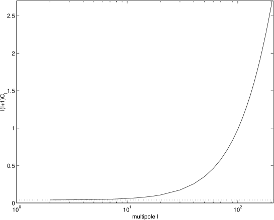
Figure 1: The multipole distributions as described by formula (25) (solid line) and formula (26) (dotted line) for the flat primordial spectrum $\beta=-2$ (${\mathrm{n}}=1$).

5 The primordial spectrum and the modulating function

A smooth spectrum of density perturbations that existed deeply in the radiation-dominated era gets strongly modified by the time of decoupling. This is the result of evolution of oscillating density perturbations (metric and plasma sound waves) through the transition from the radiation-dominated regime to the matter-dominated regime. This phenomenon is usually described with the help of the transfer function (see, for example, Peebles [1993], Efstathiou [1990], Zel’dovich & Novikov [1983], Doroshkevich & Schneider [1996], Hu & Sugiyama [1995]) and several model transfer functions are known in the literature. Their common property is a strong reduction of the short-wavelength power, starting from some large critical wavenumber. For concreteness, we shall use the transfer function derived in Grishchuk [1994]. The purpose of that paper was to derive the power spectrum from first principles and the quantum-mechanical approach was consistently used. In a moment, we shall briefly outline that derivation in order to relate notations, but the final result is not unexpected, so we shall present it first. The result is the following: instead of the strictly power-law spectrum

$$|B_{n}|^{2}=K\!(\beta)\ n^{2\beta+1}$$

introduced by equation (24), the integrals (23) for the $C_{\ell}$’s should be taken with the modified spectrum

$$|B_{n}|^{2}=K\!(\beta)\ n^{2\beta+1}M^{2}\!(n\xi_{2}),$$ (38)

where the modulating (transfer) function $M^{2}\!(n\xi_{2})$ is given by

$$M^{2}\!(n\xi_{2})=\frac{\sin^{2}\!(\frac{n\xi_{2}}{2\sqrt{3}})}{(\frac{n\xi_{2}}{2\sqrt{3}})^{2}}$$ (39)

and $\xi_{2}$ is determined by the red-shift $z_{{\mathrm{eq}}}$ at the transition from the radiation dominated era to the matter dominated era:

$$\xi_{2}=(1+z_{{\mathrm{eq}}})^{-1/2}.$$

If one does not wish to go into the details of derivation, formula (39) can be treated as a postulated phenomenological transfer function, and formula (38) as a postulated resulting spectrum.

We shall briefly outline the derivation of the power spectrum for density perturbations, but the reader interested only in applications may skip this paragraph. The theory of quantum-mechanical generation of density perturbations [1994, 1996] uses the Heisenberg operator for the field $h_{ij}(\eta,{\mathbf{x}})$:

$$h_{ij}(\eta,{\mathbf{x}})=l_{{\mathrm{Pl}}}\frac{\sqrt{16\pi}}{(2\pi)^{3/2}}\ \int_{-\infty}^{\infty}{\mathrm{d}}^{3}{\mathbf{n}}\ \frac{1}{\sqrt{2n}}\ \sum_{s=1}^{2}\stackrel{{\scriptstyle s}}{{P}}_{ij}\!({\mathbf{n}})\ \left[\stackrel{{\scriptstyle s}}{{h}}_{n}\!(\eta)\ \stackrel{{\scriptstyle s}}{{c}}_{\mathbf{n}}\!(0)\ {\mathrm{e}}^{{\mathrm{i}}{\mathbf{n\cdot x}}}+\stackrel{{\scriptstyle s}}{{h}}_{n}^{\ast}\!(\eta)\ \stackrel{{\scriptstyle s}}{{c}}_{\mathbf{n}}^{\dagger}\!(0)\ {\mathrm{e}}^{-{\mathrm{i}}{\mathbf{n\cdot x}}}\right].$$ (40)

where the Planck length $l_{{\mathrm{Pl}}}$ comes from the quantum normalisation of the field to a half of a quantum in each mode, while $c_{\mathbf{n}}\!(0)$ and $c_{\mathbf{n}}^{\dagger}\!(0)$ are the usual annihilation and creation operators. Two polarisation tensors $\stackrel{{\scriptstyle s}}{{P}}_{ij}\!\!(\mathbf{n})$ ($s=1,2$) describe, respectively, a scalar and a longitudinal component of the field:

$$\stackrel{{\scriptstyle 1}}{{P}}_{ij}\!\!({\mathbf{n}})=\delta_{ij}\ ,\ \stackrel{{\scriptstyle 2}}{{P}}_{ij}\!\!({\mathbf{n}})=-n_{i}n_{j}/n^{2}.$$

The functions $\stackrel{{\scriptstyle s}}{{h}}_{n}\!\!(\eta)$ satisfy the perturbed Einstein equations and are being evolved through three successive stages of evolution: initial (i), radiation-dominated (e) and matter-dominated (m), with the respective scale factors

$$a_{{\mathrm{i}}}(\eta) = l_{0}|\eta|^{1+\beta},\ \ \beta<-1,\ \eta\leq\eta_{1},\ \eta_{1}<0,$$

$$a_{{\mathrm{e}}}(\eta) = l_{0}a_{e}(\eta-\eta_{{\mathrm{e}}}),\ \ \eta_{1}\leq\eta\leq\eta_{2},$$ (41)

$$a_{{\mathrm{m}}}(\eta) = 2l_{H}(\eta-\eta_{{\mathrm{m}}})^{2},\ \ \eta_{2}\leq\eta\leq\eta_{{\mathrm{R}}}.$$

The constants participating in (41) are connected with each other by the continuous joining of $a(\eta)$ and $a^{\prime}(\eta)$ at the transition points. At the (m)-stage, the growing solution for $\stackrel{{\scriptstyle s}}{{h}}_{n}\!\!(\eta)$ is

$$\stackrel{{\scriptstyle 1}}{{h}}_{n}=C\!(n)\ ,\ \stackrel{{\scriptstyle 2}}{{h}}_{n}\!(\eta)=\frac{1}{10}\ C\!(n)\ [n(\eta-\eta_{{\mathrm{m}}})]^{2},$$

which allows one to relate this form of the solution with expressions (5), (7). Comparing the quantum-mechanical expectation value of the square of the generated field $h_{ij}$ with the ensemble averaging used in equation (20), one obtains $|C\!(n)|^{2}=|B_{n}|^{2}n$, where the factor $n$ comes from the extra factor $1/\sqrt{2n}$ in the definition (40). The perturbed Einstein equations plus the imposed initial conditions allow one to find the spectrum $|C\!(n)|^{2}$ from first principles, and express this quantity in terms of the participating parameters and the fundamental constants (see equations (82), (81) in Grishchuk [1994] and accompanying discussion). The resulting function $|C\!(n)|^{2}$ has the form

$$|C\!(n)|^{2}=K\!(\beta)\ n^{2\beta+2}\ M^{2}\!(n\xi_{2}),$$

where $M^{2}(n\xi_{2})$ is given by (39) and $K\!(\beta)$ is a known function of $\beta$. For the specific case of the flat spectrum, $\beta=-2$,

$$K(-2)=2\pi\ (\frac{l_{{\mathrm{Pl}}}}{l_{0}})^{2}.$$ (42)

The modulating function is an oscillatory function of $n$ and has deep minima. This can be explained [1991] as the eventual ‘desqueezing’ of some of the generated modes, and is also related to the standing wave pattern of the generated perturbations and the phenomenon of the Sakharov oscillations.

We shall now work with the function (38), leaving the parameters $\beta$, $K\!(\beta)$, $z_{{\mathrm{eq}}}$ and $z_{{\mathrm{dec}}}$ free, to be determined by the comparison with observations. In figure 2, we plot the modulating function $M^{2}\!(n\xi_{2})$.

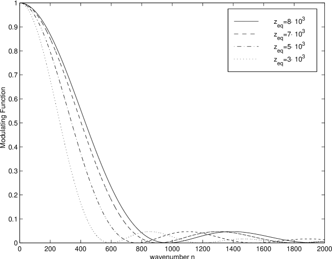
Figure 2: The modulating function $M^{2}\!(n\xi_{2})$ for different values of $z_{{\mathrm{eq}}}$. The wavenumber corresponding to the present-day Hubble radius is $4\pi$. For waves longer than and comparable to the Hubble radius, the modulating function is approximately 1. At wave-numbers around 400 the modulating function starts suppressing the primordial power spectrum significantly.

In figure 3, we present the effect of the modulating function on different primordial spectra of the density contrast, ${\mathcal{P}}\!(k)=k^{\mathrm{n}}$, which in our notation is ${\mathcal{P}}\!(n)=n^{2\beta+5}$. For sufficiently long wavelengths, the spectra retain their original form. At wave-numbers around 400 the spectra go through the maximum.

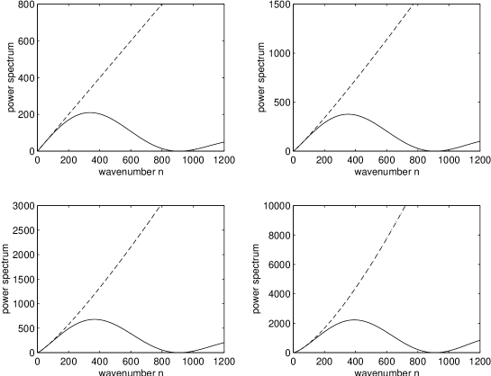
Figure 3: The effect of the modulating function on different primordial spectra $n^{2\beta+5}$. The dashed-dotted line refers to the original spectrum $n^{2\beta+5}$, while the solid one to the resulting modulated spectrum $n^{2\beta+5}\ M^{2}\!(n\xi_{2})$. The spectra shown are: i) top left hand side, the flat spectrum $\beta=-2$, ii) top right hand side, $\beta=-1.95$, iii) bottom left hand side, $\beta=-1.9$, iv) bottom right hand side, $\beta=-1.8$. All the modulated spectra were calculated for $z_{{\mathrm{eq}}}=7000$.

The maxima of the $n^{2\beta+5}\ M^{2}\!(n\xi_{2})$ spectrum, that we present in figure 3, appear at the wave-numbers which satisfy the equation

$$\left(\beta+\frac{3}{2}\right)\ \sin\!(\frac{n\xi_{2}}{2\sqrt{3}})=-\frac{n\xi_{2}}{2\sqrt{3}}\ \cos\!(\frac{n\xi_{2}}{2\sqrt{3}}).$$

The increase of $\beta$ displaces the maxima towards larger $n$. As an example, we present in figure 4 the displacement of the first maximum towards larger values of $n$, when one keeps $z_{{\mathrm{eq}}}=7000$ and increases $\beta$. The dotted line represents the right hand side of the equation (which is $\beta$-independent), while the solid, dashed-dotted and dashed lines represent the left hand side for $\beta=-2\ ,-1.9,\ -1.8$. The position of the first maximum in the power spectrum is directly related to the position of the first peak in the $\ell$-space, as will be discussed below.

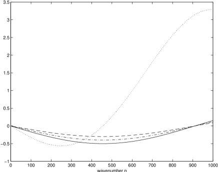
Figure 4: The dotted line shows the function $-[(n\xi_{2})/(2\sqrt{3})]\cdot\cos((n\xi_{2})/(2\sqrt{3}))$, while the solid, dashed-dotted and dashed lines show the function $[\beta+(3/2)]\cdot\sin((n\xi_{2})/(2\sqrt{3}))$ for $\beta=-2,-1.9,-1.8$ respectively. The red-shift at matter-radiation equality is taken $z_{{\mathrm{eq}}}=7000$. The values of the wavenumber where the intersection of the curves takes place (except the point $n=0$) are the points where the modulated power spectrum $n^{2\beta+5}\ M^{2}\!(n\xi_{2})$ has its first maximum. For increasing $\beta$, the first maximum occurs at larger values of $n$.

We shall now calculate numerically the multipole moments following from the formula

$$C_{\ell}=\frac{4\pi^{-1}}{100}K\!(\beta)\ \int_{0}^{\infty}\frac{{\mathrm{d}}n}{n}\ M^{2}\!(n\xi_{2})\ n^{2(\beta+2)}\ D_{\ell}^{2}\!(n),$$ (43)

which replaces formula (25).

6 The CMBR anisotropy distributions caused by density perturbations

The modulating function makes the power spectrum oscillatory and dramatically suppresses the power at short waves $n\xi_{2}\gg 1$, roughly, in proportion to $n^{-2}$. In figure 5, we present a typical graph of $\ell(\ell+1)C_{\ell}$ calculated with the modulating function. The chosen parameters are $z_{{\mathrm{dec}}}=1000$, $z_{{\mathrm{eq}}}=7000$ and $\beta=-2$. The integration in formula (43) is carried out up to $n_{{\mathrm{max}}}=1260$ and the quantity $2(2+1)C_{2}$ (for the quadrupole, $\ell=2$) is normalised to 1. The dashed-dotted line shows the result without including the modulating function. The solid line clearly shows the first peak formed due to the inclusion of the modulating function.

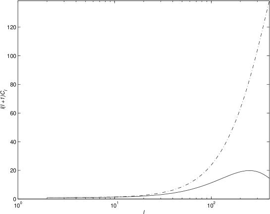
Figure 5: The quantity $\ell(\ell+1)C_{\ell}$ in the absence (dashed-dotted line) and the presence (solid line) of the modulating function.

Before proceeding to other choices of the parameters, it is instructive to explore the integrand $n^{2\beta+3}\ M^{2}\!(n\xi_{2})D^{2}_{\ell}\!(n)$ in formula (43). We shall do this for various $\ell$’s and at different intervals of integration over $n$. We shall present the graphs of the integrand, which allow one to evaluate visually the surface area under the graphs and, hence, the contributions to the integrals accumulated at different intervals of $n$.

$\ell=0$: In figure 6, we plot the integrand of $C_{0}$ at different intervals of $n$. A deep minimum of the integrand caused by the first zero of the modulating function is clearly seen. It is obvious from the graph that the integral is mostly accumulated at small $n$’s, up to $n\approx 12$ or so. Thus, the dominant contribution to $C_{0}$ comes from wavelengths larger than and comparable to the Hubble radius.

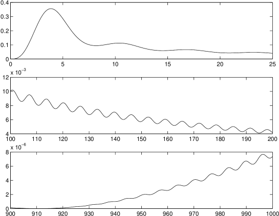
Figure 6: The integrand of the monopole moment $\ell=0$ versus the wavenumber $n$. The values of the parameters are $\beta=-2$, $z_{{\mathrm{eq}}}=7000$, $z_{{\mathrm{dec}}}=1000$.

$\ell=1$: In figure 7, we plot the integrand of $C_{1}$. The modulating function suppresses the short-wavelength power, but still leaves the dipole moment $C_{1}$ much more sensitive, than $C_{0}$ and $C_{2}$, to short waves. The remarkable fact is that the main contribution comes from wavelengths about 20–40 times shorter than the Hubble radius. For the conventional values of the Hubble parameter, this corresponds to scales around (100 - 200) Mpc., not much larger and not much smaller. The most important term in the decomposition of $D_{1}\!(n)$ (see formula (14) ), is term A. It is obvious from the graph that the numerical value of the dipole is much greater than the value of the monopole and (as we shall show below) the $\ell\geq 2$ multipoles.

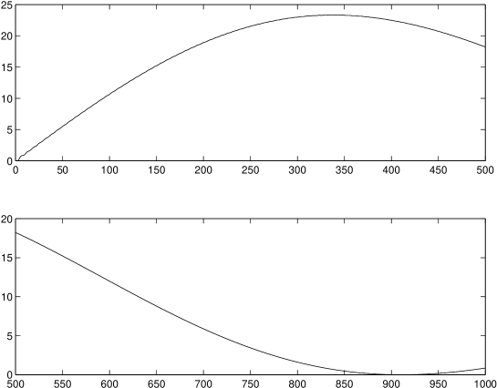
Figure 7: The integrand of the dipole moment $\ell=1$ versus the wavenumber $n$. The values of the parameters are again $\beta=-2$, $z_{{\mathrm{eq}}}=7000$, $z_{{\mathrm{dec}}}=1000$.

$\ell\geq 2$: There exists a qualitative difference between small multipoles $\ell\approx 2-10$ and relatively large multipoles $\ell\approx 100-200$, in the sense of the different roles played by terms B and D (see the decomposition of $D_{\ell\geq 2}\!(n)$ in formula (14) ). In the case of small multipoles, the dominant contribution to the integral comes from long and intermediate wavelengths, where the most important term in $D_{\ell\geq 2}\!(n)$ is term D. In the case of relatively large multipoles, the dominant contribution comes from short wavelengths, where the most important term is term B. In figures 8, 9 and 10, we present by a solid line the behaviour of the total integrands for $C_{2}$, $C_{10}$ and $C_{200}$ at different $n$’s. The values of the parameters are $z_{{\mathrm{eq}}}=7000$, $z_{{\mathrm{dec}}}=1000$ and $\beta=-2$. At the same graphs, we have also plotted with a dashed-dotted line the integrand that would result from neglecting term B, and with a dotted line the integrand that would result from neglecting term D.

From figures 8 and 9, it is evident that the dominant contribution to $C_{2}$ and $C_{10}$ comes from wavelengths longer than and comparable to the Hubble radius. In this regime, the role of term B is unimportant. Although term B will eventually dominate in the short wave regime, the contribution of that regime is negligible. At the same time, the modulating function in the most sensitive part of integration is close to 1. Therefore, the inaccurate formula (26) gives roughly correct numerical values for small multipoles. On the other hand, as figure 10 shows, the main contribution to the relatively large multipoles comes from short scales, where term B is always dominant. The neglect of term B gives wrong results.

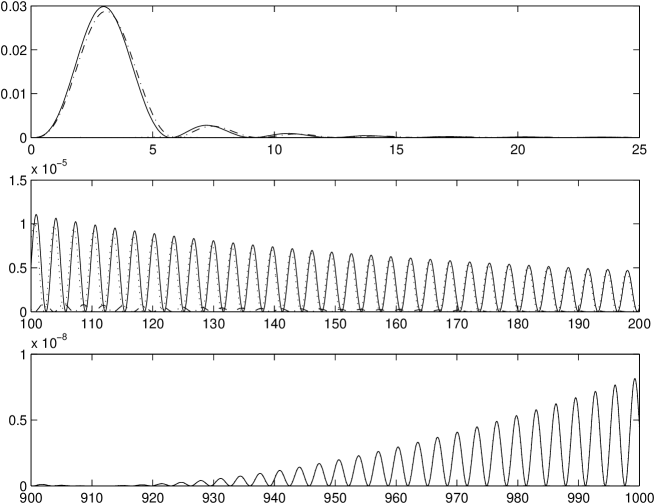
Figure 8: This plot shows by a solid line the integrand for the quadrupole moment, $\ell=2$, at different wavenumber intervals. We also display the integrand that results after retaining only term D in $D_{2}(n)$ (dashed-dotted line), and the integrand that results after retaining only term B (dotted line). For long wavelengths, term D clearly dominates over term B, while for short wavelengths the situation is reversed. At $n\sim 900$, we observe a zero caused by the first zero in the modulating function. The modulating function and the Bessel functions combine in such a manner, that the area under the curve at long and intermediate wavelengths is much greater than the area at short wavelengths, where term B dominates. The main contribution to $C_{2}$ is provided by large scales.

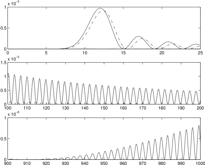
Figure 9: The same as in figure 8, for the multipole $\ell=10$. Although the role of term B is now more important than in the case of the quadrupole, the main conclusions of the $\ell=2$ case still apply to $\ell=10$.

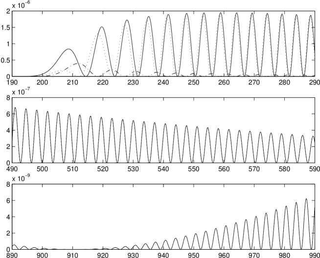
Figure 10: The same as in figure 8, for the multipole $\ell=200$. The main contribution to this multipole comes from relatively short waves, where term B dominates. The modulating term and the Bessel functions combine in such a manner, that the area under the curve at long and intermediate wavelengths is much smaller than at short wavelengths. The situation is opposite to the case of small multipoles.

Summarising, one can say the following. The major contribution to the monopole moment comes from wavelengths larger than and comparable to the Hubble radius. The actually measured isotropic temperature $T_{0}$ contains this small contribution. The major contribution to the dipole moment comes from wavelengths significantly shorter than the Hubble radius, but still far away from the onset of nonlinearities. Numerically, the dipole moment is much larger than the monopole and the $\ell\geq 2$ multipoles, as seen from the comparison of figures 6 and 8–10 with 7. To illustrate the greater sensitivity of the dipole to the short waves, one can consider the specific example of $\beta=-2$, $z_{{\mathrm{eq}}}=7000$ and $z_{{\mathrm{dec}}}=1000$. The ratio of the dipole to the quadrupole is $C_{1}/C_{2}\sim 1.4\cdot 10^{5}$. This ratio in the absence of the modulating function is $\sim 10^{6}$. The major contribution to the $\ell\in[2,20]$ multipoles comes from wavelengths longer than and comparable to the Hubble radius. The major contribution to the relatively large multipoles comes from short wavelengths, where term B dominates. Still, these multipoles are several orders of magnitude smaller than the dipole.

6.1 Variation of the parameters

We have demonstrated which wavelength regimes are responsible for the main contribution to different multipoles. While calculating the integral (43), one particular (typical) choice of the parameters has been used: $z_{{\mathrm{dec}}}=1000$, $z_{{\mathrm{eq}}}=7000$ and $\beta=-2$. One needs to explore how the change of these parameters affects the CMBR anisotropy pattern. The factor $D_{\ell}(n)$ depends on $z_{{\mathrm{dec}}}$ through the presence of $\xi$. The modulating function depends on $z_{{\mathrm{eq}}}$ through the presence of $\xi_{2}$. The primordial spectrum depends on $\beta$. We shall separately discuss the effect of the variation of $z_{{\mathrm{dec}}}$, $z_{{\mathrm{eq}}}$ and $\beta$. The results are presented in figure 11.

The effect of ${\mathbf{\mathbf{z_{{\mathrm{dec}}}}}}$: The values of the fixed parameters are $z_{{\mathrm{eq}}}=7000$ and $\beta=-2$, while we decrease $z_{{\mathrm{dec}}}$ from 1000 (solid line) to 500 (dashed-dotted line). The graph shows that the peak is displaced towards lower multipoles $\ell$, while the height of the peak increases. As already stated, the decrease of $z_{{\mathrm{dec}}}$ decreases $\xi$. This leads to the increase of term B, and explains the rise of the height of the peak. The dipole moment is insensitive to the change of $z_{{\mathrm{dec}}}$, since it is dominated by term A which is not affected by $z_{{\mathrm{dec}}}$.

The effect of ${\mathbf{\mathbf{z_{{\mathrm{eq}}}}}}$: The values of the fixed parameters are $z_{{\mathrm{dec}}}=1000$ and $\beta=-2$, while we allow $z_{{\mathrm{eq}}}$ to be 5000 (dashed-dotted line). The graph shows that the peak is displaced towards lower multipoles $\ell$, while the height of the peak decreases. The decrease of $z_{{\mathrm{eq}}}$ increases $\xi_{2}$, making the modulating function decline faster (figure 2). The $C_{\ell}$ will acquire smaller values, and therefore the values of $\ell(\ell+1)C_{\ell}$ will be smaller. This accounts for the decrease of the height of the peak. At the same time, the decrease of $z_{{\mathrm{eq}}}$ displaces the first minimum of the modulating function (and of the modulated spectrum) to smaller $n$’s (figure 2). The first maximum of the modulated power spectrum will then occur at a lower value of $n$, which translates in the displacement of the maximum of $\ell(\ell+1)C_{\ell}$ towards smaller $\ell$’s. This is the dominant reason for the first peak displacement, but we do not exclude that some additional effects can counterbalance this tendency. The decrease of $z_{{\mathrm{eq}}}$ decreases the value of the dipole. The ratio $C_{1}|_{z_{{\mathrm{eq}}}=7000}\ /\ C_{1}|_{z_{{\mathrm{eq}}}=5000}=1.25$.

The effect of ${\mathbf{\beta}}$: The values of the fixed parameters are $z_{{\mathrm{eq}}}=7000$ and $z_{{\mathrm{dec}}}=1000$, while we allow $\beta$ to be $-1.9$ (dashed-dotted line). The graph shows that the peak is displaced towards higher multipoles $\ell$, while the height of the peak increases. The displacement of the peak is explained as follows. As shown in figure 4, the increase of $\beta$ displaces the position of the first maximum of the modulated spectrum towards larger $n$. As already discussed, the change of $\beta$ does not affect the position of the minima. Therefore, the maximum of the function $\ell(\ell+1)C_{\ell}$ versus $\ell$ is displaced towards higher $\ell$. As for the increase of the height of the peak, it is explained as follows. The primordial flat spectrum $n^{2\beta+5}$ (top left graph of figure 3, dashed-dotted line) is a smooth line, growing with $n$. For a larger $\beta$, the primordial spectrum increases faster with $n$, and its plot versus $n$ is a concave curve. Therefore, the amplitudes of the modulated spectrum are larger for a larger $\beta$, which increases the values of the $C_{\ell}$ and the height of the peak. The increase of $\beta$ increases also the value of the dipole. The ratio $C_{1}|_{\beta=-1.9}\ /\ C_{1}|_{\beta=-2}\approx 3$.

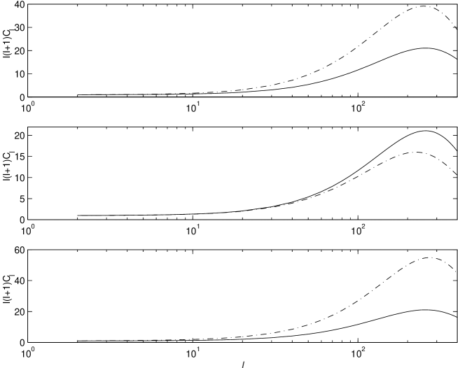
Figure 11: The effect of change of different parameters. The quantity $\ell(\ell+1)C_{\ell}$ is normalised to 1 at $\ell=2$. In all graphs, the solid line corresponds to $z_{{\mathrm{dec}}}=1000$, $z_{{\mathrm{eq}}}=7000$, $\beta=-2$. i) Top graph: the effect of decreasing $z_{{\mathrm{dec}}}$. The dashed-dotted line corresponds to $z_{{\mathrm{dec}}}=500$, $z_{{\mathrm{eq}}}=7000$, $\beta=-2$. The peak is displaced to the left and its height increases. ii) Middle graph: the effect of decreasing $z_{{\mathrm{eq}}}$. The dashed-dotted line corresponds to $z_{{\mathrm{dec}}}=1000$, $z_{{\mathrm{eq}}}=5000$, $\beta=-2$. The peak is displaced to the left and its height decreases. iii) Bottom graph: the effect of increasing $\beta$. The dashed-dotted line corresponds to $z_{{\mathrm{dec}}}=1000$, $z_{{\mathrm{eq}}}=7000$, $\beta=-1.9$. The peak is displaced to the right and its height increases.

6.2 The inclusion of intrinsic anisotropies

The derivation of the starting formula (3) is based on solving the differential equation for the photons’ geodesics [1967]. As usual, when defining a solution, one should indicate the initial conditions. In our problem, this translates into the intrinsic CMBR anisotropies. These anisotropies reflect the temperature inhomogeneities already present on the last scattering surface. There are many elaborate treatments dealing with this subject (for example, Doroshkevich & Schneider [1996], Hu & Sugiyama [1995]). We shall use a simplified model (see, e.g. Padmanabhan [1993]), where the intrinsic anisotropy is related to the radiation density contrast by the simple relationship

$$\left(\frac{\delta T}{T}\right)_{{\mathrm{in}}}=\frac{1}{4}\left.\left(\frac{\delta\rho}{\rho}\right)_{{\mathrm{rad}}}\right|_{\eta=\eta_{{\mathrm{E}}}}.$$

Deeply in the radiation-dominated era, photons are tightly coupled to baryons through Thomson scattering. It can be seen that the radiation density contrast can be related to the baryon density contrast by

$$\left(\frac{\delta\rho}{\rho}\right)_{{\mathrm{rad}}}=\frac{4}{3}\left(\frac{\delta\rho}{\rho}\right)_{{\mathrm{b}}}.$$

Assuming that the dominant matter component governing the scale factor at the matter-dominated stage is a sort of dark matter, the baryon density contrast can be related to the dark matter density contrast by

$$\left(\frac{\delta\rho}{\rho}\right)_{{\mathrm{b}}}=\frac{z_{{\mathrm{dec}}}}{z_{{\mathrm{eq}}}}\ \left(\frac{\delta\rho}{\rho}\right)_{{\mathrm{dm}}}.$$

Therefore, one can relate the intrinsic anisotropies to the total density variation at the last scattering surface:

$$\left(\frac{\delta T}{T}\right)_{{\mathrm{in}}}=\frac{1}{3}\frac{z_{{\mathrm{dec}}}}{z_{{\mathrm{eq}}}}\ \left.\left(\frac{\delta\rho}{\rho}\right)\right|_{\eta=\eta_{{\mathrm{E}}}}.$$

This intrinsic part should be added to the gravitational part of the previous Sections, and this total temperature variation should be decomposed over spherical harmonics. One then repeats the procedure already performed in the absence of the intrinsic anisotropy, to derive the full formula (containing both gravitational and intrinsic parts) for the multipole moments $C_{\ell}$. This is again equation (43), where the expression (13) for $D_{\ell}(n)$ is modified to

$$D_{\ell}(n)=\frac{1}{3}\ n\ \delta_{\ell 1}+n(1-\xi)\ \frac{1}{2\ell+1}[(\ell+1)\ j_{\ell+1}\!(n\xi)-\ell\ j_{\ell-1}\!(n\xi)]+\delta_{\ell 0}-\left[1+\frac{3}{10}\ \frac{1}{6}\ (n\xi_{2})^{2}\right]\ j_{\ell}(n\xi).$$ (44)

The inclusion of the intrinsic part causes the further increase of the multipole moments $C_{\ell}$, and the increase of the height of the first peak in the CMBR distribution. If plasma fluid at the last scattering surface retains appreciable velocity with respect to chosen by us coordinate system, which is synchronous and comoving with gravitationally dominant matter, this will give rise to further corrections. As will be argued in the next Section, the observed first peak seems already to be too high to be explained, together with other multipoles, by density perturbations alone.

7 A first comparison with observations

The current CMBR observational results can be summarised as follows.

1) The COBE observations [1996] have shown the presence of a ‘plateau’ in the multipole region $\ell\in[2,20]$. As a characteristic value in this region, we shall use the quantity $\ell(\ell+1){\mathbf{C}}_{\ell}|_{\ell=10}$. By the bold-face symbol ${\mathbf{C}}_{\ell}$ we denote the value of the multipole moment $\ell$ that follows from observations. (The lack of ergodicity on a 2-sphere [1997] prevents one from precise extraction of statistical $C_{\ell}$ from a single, even if arbitrarily accurate, map of the sky, but this is not a matter of concern for us here.) The COBE result shows that

$$\sqrt{\frac{\ell(\ell+1){\mathbf{C}}_{\ell}|_{\ell=10}}{2\pi}}\cdot T_{0}=27.7^{+3.9}_{-4.5}\ {\mathrm{\mu K}},$$

where $T_{0}$ is the background, isotropic, temperature of the CMBR. This gives the value of $\ell(\ell+1){\mathbf{C}}_{\ell}|_{\ell=10}$:

$$\ell(\ell+1){\mathbf{C}}_{\ell}|_{\ell=10}\approx 6.4\cdot 10^{-10}.$$ (45)

2) The dipole anisotropy was also measured by COBE. According to Bennett et al. [1996],

$$\sqrt{\frac{(2\ell+1){\mathbf{C}}_{\ell}|_{\ell=1}}{4\pi}}\cdot T_{0}=3.353\pm 0.024\ {\mathrm{mK}},$$

leading to

$${\mathbf{C}}_{1}\approx 6.3\cdot 10^{-6}.$$ (46)

3) All the CMBR observations performed at the region of higher $\ell$’s have suggested the presence of a peak. The most recent and accurate experiments BOOMERanG [2000] and MAXIMA-1 [2000] gave the location and height of this peak with some precision. According to these results, the peak is located at $200\leq\ell_{{\mathrm{peak}}}\leq 220$, with $\sqrt{\ell(\ell+1){\mathbf{C}}_{\ell}|_{{\mathrm{peak}}}/(2\pi)}\cdot T_{0}$ having the value $69\pm 8\ {\mathrm{\mu K}}$ [2000] or $78\pm 6\ {\mathrm{\mu K}}$ [2000]. For the sake of this discussion, we adopted the values of Hanany et al. [2000],

$$\ell_{{\mathrm{peak}}}\simeq 220$$ (47)

and

$$\sqrt{\frac{\ell(\ell+1){\mathbf{C}}_{\ell}|_{{\mathrm{peak}}}}{2\pi}}\cdot T_{0}=78\pm 6\ {\mathrm{\mu K}}.$$

Therefore, we shall use as a characteristic value in this region the quantity

$$\ell(\ell+1){\mathbf{C}}_{\ell}|_{{\mathrm{peak}}}\approx 5.1\cdot 10^{-9}.$$ (48)

We accept the position of the peak (47), and we regard the three numbers (48), (46), (45) as three observational points to which we try to fit (admittedly, in a somewhat simplistic manner) the theoretical curves. The curves for $\ell(\ell+1)C_{\ell}$ are constructed with the help of formulae (43) and (44), where the upper limit of integration is taken at $n_{{\mathrm{max}}}=1260$. The strategy of the fitting is as follows.

There are several combinations of the parameters $(z_{{\mathrm{eq}}},\ z_{{\mathrm{dec}}},\ \beta)$ (some of them are listed in table 1) for which the position of the peak is at (47) and the height of the peak is at (48). At the same time, we check that the calculated statistical dipole is close (deviation less than 5 per cent) to the observed value (46). A drastic adjustment of the calculated dipole with the help of a ‘peculiar’ velocity of the individual observer, that is, allowing the observer to move with a large velocity with respect to the matter-dominated fluid (i.e. with respect to the comoving coordinate system) seems to be artificial. As the statistical dipole is already quite large, it seems especially unnatural to try to do this. As a guideline in the choice of $z_{{\mathrm{dec}}}$ and $z_{{\mathrm{eq}}}$, we use the fact that $z_{{\mathrm{dec}}}$ should be close to $1000$ and $z_{{\mathrm{eq}}}$ should be somewhere near to $10^{4}$. The decoupling red-shift $z_{{\mathrm{dec}}}$ certainly depends on the baryon content of the Universe $\Omega_{b}$, but it can also depend on a complicated ionisation history of the decoupling era. The equality red-shift $z_{{\mathrm{eq}}}$ certainly depends on the total matter content of the Universe (baryons, cold dark matter, etc.) but it also depends on its radiation content (CMB photons, possible contribution of massless neutrinos, etc.). In addition, the total density parameter $\Omega$ can also deviate from the postulated here $\Omega=1$. This may change $z_{{\mathrm{eq}}}$ without seriously affecting our solutions for the gravitational field perturbations $h_{ij}$ and subsequent formulae, derived, strictly speaking, for the case $\Omega=1$. It would be a difficult problem to try to decipher all the relevant quantities from just the two numbers $z_{{\mathrm{dec}}}$ and $z_{{\mathrm{eq}}}$. However, we will operate with these parameters, since this is what the calculations immediately require us to specify. As for $\beta$, we have considered the three different cases $\beta=$ $-2$, $-1.95$, $-1.9$. Since $K\!(\beta)$ is not very sensitive to $\beta$ in this interval, we have used one and the same formula (42) for all the three cases. Then, every fit of the peak and the dipole to their observed values defines its own value for the ratio $\Lambda\equiv(l_{{\mathrm{Pl}}}/l_{0})^{2}$ and for the calculated quantity $\ell(\ell+1)C_{\ell}|_{\ell=10}$. This quantity is finally compared with the observed value (45). The result of this comparison shows that the theoretical $\ell(\ell+1)C_{\ell}|_{\ell=10}$ is systematically smaller than the observed $\ell(\ell+1){\mathbf{C}}|_{\ell=10}$, for all considered combinations of the parameters $(z_{{\mathrm{eq}}},\ z_{{\mathrm{dec}}},\ \beta)$. The observational points should be surrounded by their error bars, but in order not to proliferate the already existing uncertainties, we focus on the mean values. One can say that, despite of the still allowed variation of the parameters, the calculated ‘plateau’ is persistently lower than it should be. These calculations are visualised in figure 12.

We believe that this deficit at small multipoles serves as an indication that density perturbations alone can hardly be responsible for all of the CMBR anisotropies. The most natural way to proceed is to include gravitational waves and repeat this scheme.

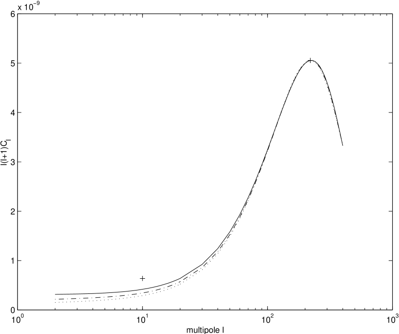
Figure 12: Comparison of theoretical models, based on density perturbations only, with observations. The solid line corresponds to the set of parameters $(5000,1000,-2)$, the dashed-dotted to $(4500,1000,-1.95)$ and the dotted to $(4000,1000,-1.9)$. The crosses show the observed values of $\ell(\ell+1){\mathbf{C}}|_{\ell=10}$ and $\ell(\ell+1){\mathbf{C}}_{\ell}|_{{\mathrm{peak}}}$. By fitting the theoretical peak to the observed peak, we notice that there is a deficit at the plateau.

Table 1: Comparison of some theoretical models, strictly satisfying the requirements on the position and the height of the first peak, with observations.

$z_{{\mathrm{eq}}}$	$z_{{\mathrm{dec}}}$	$\beta$	$\Lambda$	$\ell(\ell+1)C_{\ell}|_{\ell=10}$	${\mathbf{C}}_{10}/C_{10}$	$C_{1}$	${\mathbf{C}}_{1}/C_{1}$
5000	1000	-2.00	$7.7\cdot 10^{-9}$	$4.2\cdot 10^{-10}$	1.5	$6.1\cdot 10^{-6}$	1.04
4500	1000	-1.95	$5.0\cdot 10^{-9}$	$3.4\cdot 10^{-10}$	1.9	$6.1\cdot 10^{-6}$	1.03
4000	1000	-1.90	$3.3\cdot 10^{-9}$	$2.9\cdot 10^{-10}$	2.2	$6.1\cdot 10^{-6}$	1.03

8 The gravitational wave contribution to the CMBR anisotropies

Gravitational waves are inevitably generated by the strong variable gravitational field of the early Universe (see, for example, Grishchuk et al. [2000] and references therein). The preliminary calculations show [1994] that the contribution of quantum-mechanically generated gravitational waves to the small multipoles should be of the same order of magnitude and, numerically, somewhat larger than the contribution of density perturbations generated by the same mechanism. In this paper, however, we follow a phenomenological approach and do not not focus on the origin of cosmological perturbations and consequences of the particular generating mechanism. We introduce, instead, a phenomenological parameter $\varpi$, which regulates the relative contributions of gravitational waves and density perturbations. In effect, we want to find the value of $\varpi$ which allows to raise the plateau in figure 12 to the observationally required level, at the expense of gravitational waves. At the same time, the fits to the peak and the dipole are required to be as good as before. It is already clear from table 1 and figure 12 that the required amount of gravitational waves, as compared with density perturbations, is within a factor of 2 at $\ell=10$. This seems to be in agreement with theoretical expectations, but we shall go into a more detailed analysis in Section 9.

In this paragraph, we shall only remind the fundamentals about primordial gravitational waves. Although we follow the quantum mechanical derivation, the final formula (51) for $C_{\ell}$ is true (up to the overall numerical coefficient) for a broad class of gravitational waves. The Heisenberg operator for the gravitational wave metric perturbations is

$$h_{ij}(\eta,{\mathbf{x}})=l_{{\mathrm{Pl}}}\frac{\sqrt{16\pi}}{(2\pi)^{3/2}}\ \int_{-\infty}^{\infty}{\mathrm{d}}^{3}{\mathbf{n}}\ \frac{1}{\sqrt{2n}}\ \sum_{s=1}^{2}\ \stackrel{{\scriptstyle s}}{{p}}_{ij}\!\!({\mathbf{n}})\ \left[\stackrel{{\scriptstyle s}}{{h}}_{n}\!\!(\eta)\ \stackrel{{\scriptstyle s}}{{c}}_{{\mathbf{n}}}\!\!(0)\ {\mathrm{e}}^{{\mathrm{i}}{\mathbf{n\cdot x}}}+\stackrel{{\scriptstyle s}}{{h}}_{n}\!\!\!\!\!^{\ast}(\eta)\ \stackrel{{\scriptstyle s}}{{c}}_{{\mathbf{n}}}\!\!\!\!\!^{\dagger}(0)\ {\mathrm{e}}^{-{\mathrm{i}}{\mathbf{n\cdot x}}}\right],$$ (49)

where, again, $l_{{\mathrm{Pl}}}$ comes from quantum normalisation, and the transverse traceless polarisation tensors $\stackrel{{\scriptstyle s}}{{p}}_{ij}\!\!({\mathbf{n}})$ satisfy the relations

$$\stackrel{{\scriptstyle s}}{{p}}_{ij}\!\!({\mathbf{n}})\ \stackrel{{\scriptstyle s^{\prime}}}{{p}}\!\!^{ij}\!({\mathbf{n}})=2\delta_{ss^{\prime}},\ \stackrel{{\scriptstyle s}}{{p}}_{ij}\!\!({\mathbf{n}})=\stackrel{{\scriptstyle s}}{{p}}_{ij}\!\!({\mathbf{-n}}),\ \stackrel{{\scriptstyle s}}{{p}}_{ij}n^{j}=0,\ \stackrel{{\scriptstyle s}}{{p}}_{ij}\delta^{ij}=0.$$

The time evolution of each of the amplitudes $h_{n}\!(\eta)$ for $s=1,\ 2$ is given by one and the same equation with the same initial conditions, so one deals with one and the same $h_{n}\!(\eta)$. After solving for $h_{n}\!(\eta)$ at the three stages (41) and continuously joining the solutions, one arrives at a ‘growing’ and a ‘decaying’ solution in the matter-dominated era. The growing solution is given by the expression

$$h_{n}\!(\eta)\approx{\mathrm{i}}\ {\mathrm{e}}^{{\mathrm{i}}n\eta_{0}}\ 3\Psi\!(\beta)\ (-1)^{-\beta}\ l_{0}^{-1}\ n^{\beta+1}\ \frac{j_{1}\!(n(\eta-\eta_{m}))}{n(\eta-\eta_{m})},$$ (50)

where the quantity $|\Psi\!(\beta)|^{2}$ is unity for $\beta=-2$, and we neglect its weak $\beta$-dependence for other values of $\beta$ considered here. For a reference, $|\Psi\!(\beta)|^{2}$ is related with $K\!(\beta)$ discussed in Section 4 by

$$K\!(\beta)=2\pi|\Psi\!(\beta)|^{2}\left(\frac{l_{{\mathrm{Pl}}}}{l_{0}}\right)^{2}.$$

Combining (50) with (49), using the Sachs-Wolfe formula (3), and repeating the same steps that have led to the formula for $C_{\ell}$’s caused by density perturbations, one arrives at [1993]

$$C_{\ell}\approx 4\cdot 9|\Psi\!(\beta)|^{2}\ \left(\frac{l_{{\mathrm{Pl}}}}{l_{0}}\right)^{2}\ (\ell-1)\ell(\ell+1)(\ell+2)\int_{0}^{+\infty}n^{2(\beta+2)}\ f_{\ell}(n)\ \frac{{\mathrm{d}}n}{n},$$ (51)

where

$$f_{\ell}(n)\equiv\left|\int_{0}^{n\xi}\frac{j_{\ell}\!(x)}{x^{2}}\ \frac{j_{2}\!(n-x)}{(n-x)}{\mathrm{d}}x\right|^{2}.$$

As (51) shows, gravitational waves contribute to multipoles $\ell\geq 2$, in contrast to primordial density perturbations, which contribute to all multipoles.

We shall now present the multipole moments caused by gravitational waves. The solid line in both graphs of figure 13, shows the behaviour of $\ell(\ell+1)C_{\ell}$ versus $\ell$ for $z_{{\mathrm{eq}}}=7000$, $z_{{\mathrm{dec}}}=1000$ and $\beta=-2$. The quantity $\ell(\ell+1)C_{\ell}|_{\ell=2}$ is normalised to 1. The higher order multipoles are negligible in comparison with the lower order ones, unlike the case of density perturbations. This is expected because of the different behaviour of the short wavelength density perturbations and gravitational waves. At the matter-dominated stage, short wavelength density perturbations increase with time as $\eta^{2}$, while short wavelength gravitational waves decrease with time as $\eta^{-2}$. Figure 13 also shows the effects of the variation of different parameters. As expected, in all cases, gravitational waves mostly contribute to the small multipoles.

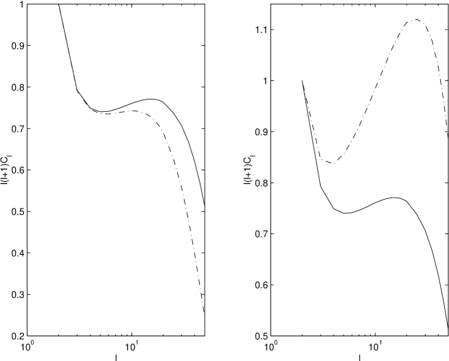
Figure 13: The effect of the variation of the different parameters on $\ell(\ell+1)C_{\ell}$. In both graphs, the solid line corresponds to $z_{{\mathrm{dec}}}=1000,\ z_{{\mathrm{eq}}}=7000,\ \beta=-2$. i) Left graph: the effect of decreasing $z_{{\mathrm{dec}}}$. The dashed-dotted line corresponds to $z_{{\mathrm{dec}}}=500,\ z_{{\mathrm{eq}}}=7000,\ \beta=-2$. ii) Right graph: the effect of increasing $\beta$. The dashed-dotted line corresponds to $z_{{\mathrm{dec}}}=1000,\ z_{{\mathrm{eq}}}=7000,\ \beta=-1.9$. The local maximum is displaced to the right and its height increases, exceeding the value of $\ell(\ell+1)C_{\ell}|_{\ell=2}$.

9 A second comparison with observations - Conclusions

We denote by $C^{{\mathrm{dp}}}_{\ell}$ and $C^{{\mathrm{gw}}}_{\ell}$ the multipole moments induced by density perturbations and gravitational waves, respectively. $C^{{\mathrm{dp}}}_{\ell}$ is given by (43), whereas $C^{{\mathrm{gw}}}_{\ell}$ is given by (51). We introduce a numerical parameter $\varpi$ in such a way that the total $\ell(\ell+1)C_{\ell}$ is given by

$$\ell(\ell+1)C_{\ell}=\ell(\ell+1)[C^{{\mathrm{gw}}}_{\ell}+\varpi\cdot C^{{\mathrm{dp}}}_{\ell}].$$ (52)

The value of $\varpi$ would be strictly 1, if one could guarantee that the idealised model that has led to formulae (43), (51) has accurately taken into account all physical processes that might have affected density perturbations and gravitational waves throughout their entire evolution, from the moment they existed in a vacuum quantum state and up to the era of decoupling of CMB radiation from matter. Since one may have legitimate doubts in such accuracy, the correction parameter $\varpi$ may be thought of as a measure of a necessary modification (but only in the form of an overall numerical coefficient) to our theoretical framework.

As was shown in Section 8, gravitational waves do not contribute to the dipole, and do not practically contribute to the peak. Therefore, we require the quantity $\varpi\cdot\ell(\ell+1)C^{{\mathrm{dp}}}_{\ell}|_{{\mathrm{peak}}}$ to be equal to the characteristic value (48). At the same time, we require $\ell(\ell+1)C_{\ell}|_{\ell=10}$, defined by setting $\ell=10$ in (52), to be equal to the characteristic value (45). This comparison revises the ratio $\Lambda=(l_{{\mathrm{Pl}}}/l_{0})^{2}$ and determines the parameter $\varpi$. We then construct the ratio $\ell(\ell+1)C^{{\mathrm{gw}}}_{\ell}|_{\ell=10}/(\varpi\cdot\ell(\ell+1)C_{\ell}^{{\mathrm{dp}}}|_{\ell=10})=C^{{\mathrm{gw}}}_{10}/(\varpi\cdot C^{{\mathrm{dp}}}_{10})$, which shows the relative contributions of gravitational waves and density perturbations to the small multipoles. Finally, we compare the value $\varpi\cdot C_{1}$ with the observed value (46) of the dipole. The results of this analysis are shown in table 2, while a visual representation is given in figure 14.

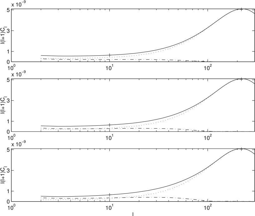
Figure 14: Comparison of the theoretical model, including density perturbations and gravitational waves, with observations. The dotted line shows the contribution of the corrected density perturbations alone, the dashed-dotted line shows the contribution of gravitational waves alone, and the solid line is the total $\ell(\ell+1)C_{\ell}$. The top graph corresponds to the set of parameters $(5000,1000,-2)$, the middle graph to $(4500,1000,-1.95)$, and the bottom graph to $(4000,1000,-1.9)$. The crosses, again, correspond to the observed values of $\ell(\ell+1){\mathbf{C}}|_{\ell=10}$ and $\ell(\ell+1){\mathbf{C}}|_{{\mathrm{peak}}}$. In all cases, the contribution of gravitational waves to the plateau is comparable to that of density perturbations, and for larger values of $\beta$ the contribution of gravitational waves is numerically greater than that of density perturbations.

Table 2: Comparison of the theoretical model with observations, for the sets of parameters $(5000,1000,-2)$, $(4500,1000,-1.95)$ and $(4000,1000,-1.9)$. Primordial gravitational waves have now been taken into account. The position and the height of the first peak, as well as the dipole moment and the plateau, are in an excellent fit to the observations.

$z_{{\mathrm{eq}}}$	$z_{{\mathrm{dec}}}$	$\beta$	$\Lambda$	$\varpi$	$\varpi\cdot\ell(\ell+1)C^{{\mathrm{dp}}}_{\ell}|_{\ell=10}$	$\ell(\ell+1)C^{{\mathrm{gw}}}_{\ell}|_{\ell=10}$	$C^{{\mathrm{gw}}}_{10}/(\varpi\cdot C^{{\mathrm{dp}}}_{10})$	$\varpi\cdot C^{{\mathrm{dp}}}_{1}$	${\mathbf{C}}_{1}/(\varpi\cdot C^{{\mathrm{dp}}}_{1})$
5000	1000	-2.00	$2.6\cdot 10^{-10}$	29.2	$4.1\cdot 10^{-10}$	$2.2\cdot 10^{-10}$	0.5	$6.1\cdot 10^{-6}$	1.04
4500	1000	-1.95	$2.9\cdot 10^{-10}$	17.2	$3.4\cdot 10^{-10}$	$2.9\cdot 10^{-10}$	0.8	$6.1\cdot 10^{-6}$	1.03
4000	1000	-1.90	$2.8\cdot 10^{-10}$	11.6	$2.9\cdot 10^{-10}$	$3.4\cdot 10^{-10}$	1.2	$6.1\cdot 10^{-6}$	1.03

To summarise, we have revised the formula (1) for $C_{\ell}$’s caused by density perturbations and derived the corrected expression (43). We have shown that the monopole moment $C_{0}$ is actually finite and small, while the dipole moment is very sensitive to short wavelengths. Because of that, the dipole moment is much larger than the $\ell=0$ and $\ell\geq 2$ multipoles. We have then proceeded to the multipoles $\ell\geq 2$. The correct formula predicts growth of the function $\ell(\ell+1)C_{\ell}$ with $\ell$. We have illustrated how the presence of the modulating function $M^{2}\!(n\xi_{2})$ gives rise to the first peak in the CMBR anisotropy pattern produced by density perturbations. (It would be nice to see further peaks discovered in the positions and with the heights suggested by the modulating function, but this is the domain of wavelengths where many other physical processes may intervene.) A first comparison with observations has indicated that the observed multipoles can hardly be explained by density perturbations alone, because of the deficit in the small $\ell$ plateau. We took a step further and included primordial gravitational waves. This inclusion gives a picture in better agreement with observations. We explored the cases $\beta>-2$ which make the primordial spectrum a little bit ‘blue’, thus allowing to avoid the infrared divergence of the primordial perturbations that occurs for $\beta\leq-2$ (see (20) and (24)). We conclude that models with $\beta>-2$, and therefore with larger contributions of gravitational waves, are better than a model without gravitational waves and with the flat spectrum $\beta=-2$. This analysis is complementary to other studies of the CMBR data [2000, 2000a, 2000b, 2000, 2000, 2000, 2000, 2000, 2000, 2000, 2000, 2000, 2000, 2000, 2000, 2000a, 2000b], not all of which, though, seem to agree with each other.

10 Acknowledgements

The authors are grateful to A. Doroshkevich, G. Smoot, L. Piccirillo and P. Mauskopf for useful discussions and correspondence. A. Dimitropoulos was supported by the Foundation of State Scholarships of Greece.

Appendix A Outline of the calculation of the contribution of term II

We need to prove that the contribution of term II to formula (9) is given by

$${\mathrm{g}}_{\ell m}=\frac{4\pi}{(2\pi)^{3/2}}\ {\mathrm{i}}^{\ell}\ \int_{-\infty}^{+\infty}{\mathrm{d}}^{3}{\mathbf{n}}\ B\!_{\mathbf{n}}\ n(1-\xi)\ \frac{1}{2\ell+1}[(\ell+1)\ j_{\ell+1}\!(n\xi)-\ell\ j_{\ell-1}\!(n\xi)]\ Y_{\ell m}^{\ast}\!(\Theta,\Phi).$$ (53)

The starting point of the calculation is the expression

$$G_{II}\!({\mathbf{e}})=\frac{1}{(2\pi)^{3/2}}\ \int_{-\infty}^{+\infty}{\mathrm{d}}^{3}{\mathbf{n}}\ B\!_{\mathbf{n}}\ (-{\mathrm{i}})\ {\mathbf{n\cdot e}}\ (1-\xi)\ {\mathrm{e}}^{{\mathrm{i}}{\mathbf{n\cdot e}}\xi}$$ (54)

which needs to be presented as

$$G_{II}\!({\mathbf{e}})=\sum_{\ell=0}^{\infty}\sum_{m=-\ell}^{\ell}{\mathrm{g}}_{\ell m}\ Y_{\ell m}\!(\theta,\phi).$$ (55)

Using the representations (2) and (10) in the scalar product ${\mathbf{n\cdot e}}$, the spherical wave expansion of a plane wave (11), and the explicit form of $Y_{1f}(\theta,\phi)$ (see e.g. page 99 of Jackson [1975]) we derive:

$${\mathrm{i}}{\mathbf{n\cdot e}}\ (1-\xi)\ {\mathrm{e}}^{{\mathrm{i}}{\mathbf{n\cdot e}}\xi}=4\pi\ \sum_{\ell=0}^{\infty}\sum_{m=-\ell}^{\ell}\sum_{f=-1}^{1}{\mathrm{i}}^{\ell+1}\ \frac{4\pi}{3}\ n(1-\xi)\ Y^{\ast}_{1f}(\Theta,\Phi)\ Y^{\ast}_{\ell m}\!(\Theta,\Phi)\ Y_{1f}(\theta,\phi)\ Y_{\ell m}\!(\theta,\phi).$$ (56)

We now equate the right hand sides of (54) and (55), multiply the resulting expression with $Y_{\ell^{\prime}m^{\prime}}^{\ast}(\theta,\phi)$, and use the orthogonality condition of the spherical harmonics (e.g. formula (3.55) in Jackson [1975]). This allows one to write

$${\mathrm{g}}_{\ell^{\prime}m^{\prime}}=\stackrel{{\scriptstyle 1}}{{{\mathrm{g}}}}_{\ell^{\prime}m^{\prime}}+\stackrel{{\scriptstyle 2}}{{{\mathrm{g}}}}_{\ell^{\prime}m^{\prime}}+\stackrel{{\scriptstyle 3}}{{{\mathrm{g}}}}_{\ell^{\prime}m^{\prime}}$$ (57)

where

$$\stackrel{{\scriptstyle 1}}{{{\mathrm{g}}}}_{\ell^{\prime}m^{\prime}} = \frac{4\pi}{(2\pi)^{3/2}}\ \sum_{\ell=0}^{\infty}\sum_{m=-\ell}^{\ell}\frac{4\pi}{3}\ {{\mathrm{i}}}^{\ell+3}\ \int_{-\infty}^{+\infty}{\mathrm{d}}^{3}{\mathbf{n}}\ B\!_{\mathbf{n}}\ n(1-\xi)\ j_{\ell}\!(n\xi)\ Y_{1,-1}^{\ast}\!(\Theta,\Phi)\ Y_{\ell m}^{\ast}\!(\Theta,\Phi)\cdot$$ (58)

$$\cdot\int_{0}^{\pi}\int_{0}^{2\pi}Y_{1,-1}\!(\theta,\phi)\ Y_{\ell m}\!(\theta,\phi)\ Y_{\ell^{\prime}m^{\prime}}^{\ast}\!(\theta,\phi)\ \sin\!\theta\ {\mathrm{d}}\theta\ {\mathrm{d}}\phi$$

$$\stackrel{{\scriptstyle 2}}{{{\mathrm{g}}}}_{\ell^{\prime}m^{\prime}} = \frac{4\pi}{(2\pi)^{3/2}}\ \sum_{\ell=0}^{\infty}\sum_{m=-\ell}^{\ell}\frac{4\pi}{3}\ {\mathrm{i}}^{\ell+3}\ \int_{-\infty}^{+\infty}{\mathrm{d}}^{3}{\mathbf{n}}\ B\!_{\mathbf{n}}\ n(1-\xi)\ j_{\ell}\!(n\xi)\ Y_{10}^{\ast}\!(\Theta,\Phi)\ Y_{\ell m}^{\ast}\!(\Theta,\Phi)\cdot$$ (59)

$$\cdot\int_{0}^{\pi}\int_{0}^{2\pi}Y_{10}\!(\theta,\phi)\ Y_{\ell m}\!(\theta,\phi)\ Y_{\ell^{\prime}m^{\prime}}^{\ast}\!(\theta,\phi)\ \sin\!\theta\ {\mathrm{d}}\theta\ {\mathrm{d}}\phi$$

$$\stackrel{{\scriptstyle 3}}{{{\mathrm{g}}}}_{\ell^{\prime}m^{\prime}} = \frac{4\pi}{(2\pi)^{3/2}}\ \sum_{\ell=0}^{\infty}\sum_{m=-\ell}^{\ell}\frac{4\pi}{3}\ {\mathrm{i}}^{\ell+3}\ \int_{-\infty}^{+\infty}{\mathrm{d}}^{3}{\mathbf{n}}\ B\!_{\mathbf{n}}\ n(1-\xi)\ j_{\ell}\!(n\xi)\ Y_{11}^{\ast}\!(\Theta,\Phi)\ Y_{\ell m}^{\ast}\!(\Theta,\Phi)\cdot$$ (60)

$$\cdot\int_{0}^{\pi}\int_{0}^{2\pi}Y_{11}\!(\theta,\phi)\ Y_{\ell m}\!(\theta,\phi)\ Y_{\ell^{\prime}m^{\prime}}^{\ast}\!(\theta,\phi)\ \sin\!\theta\ {\mathrm{d}}\theta\ {\mathrm{d}}\phi.$$

In each of (58)-(60), we decompose the spherical harmonics into associated Legendre functions (formula (3.53) of Jackson [1975]), perform the integration over $\theta$ and $\phi$, utilising formulae (8.733.2)-(8.733.4) of Gradshteyn & Ryzhik [1980] and the orthogonality condition of the associated Legendre functions (formula (3.52) of Jackson [1975]), and find these expressions to give

$$\stackrel{{\scriptstyle 1}}{{{\mathrm{g}}}}_{\ell^{\prime}m^{\prime}} = \frac{4\pi}{(2\pi)^{3/2}}\ {\mathrm{i}}^{\ell^{\prime}+2}\ \int_{-\infty}^{+\infty}{\mathrm{d}}^{3}{\mathbf{n}}\ B\!_{\mathbf{n}}\ n(1-\xi)\ \sqrt{\frac{2\ell^{\prime}+1}{4\pi}\ \frac{(\ell^{\prime}-m^{\prime})!}{(\ell^{\prime}+m^{\prime})!}}\ \frac{1}{2\ell^{\prime}+1}\cdot$$ (61)

$$\cdot\left[j_{\ell^{\prime}+1}\!(n\xi)\ \frac{\sqrt{1-{\mathcal{B}}^{2}}}{2}\ P_{\ell^{\prime}+1}^{m^{\prime}+1}\!({\mathcal{B}})+j_{\ell^{\prime}-1}\!(n\xi)\ \frac{\sqrt{1-{\mathcal{B}}^{2}}}{2}\ P_{\ell^{\prime}-1}^{m^{\prime}+1}\!({\mathcal{B}})\right]\ {\mathrm{e}}^{-{\mathrm{i}}m^{\prime}\Phi}$$

$$\stackrel{{\scriptstyle 2}}{{{\mathrm{g}}}}_{\ell^{\prime}m^{\prime}} = \frac{4\pi}{(2\pi)^{3/2}}\ {\mathrm{i}}^{\ell^{\prime}+2}\int_{-\infty}^{+\infty}{\mathrm{d}}^{3}{\mathbf{n}}\ B\!_{\mathbf{n}}\ n(1-\xi)\ \sqrt{\frac{2\ell^{\prime}+1}{4\pi}\ \frac{(\ell^{\prime}-m^{\prime})!}{(\ell^{\prime}+m^{\prime})!}}\ \frac{1}{2\ell^{\prime}+1}\cdot$$ (62)

$$\cdot\left[j_{\ell^{\prime}+1}\!(n\xi)\ [-(\ell^{\prime}-m^{\prime}+1)]\ {\mathcal{B}}\ P_{\ell^{\prime}+1}^{m^{\prime}}\!({\mathcal{B}})+j_{\ell^{\prime}-1}\!(n\xi)\ (\ell^{\prime}+m^{\prime})\ {\mathcal{B}}\ P_{\ell^{\prime}-1}^{m^{\prime}}\!({\mathcal{B}})\right]\ {\mathrm{e}}^{-{\mathrm{i}}m^{\prime}\Phi}$$

$$\stackrel{{\scriptstyle 3}}{{{\mathrm{g}}}}_{\ell^{\prime}m^{\prime}} = \frac{4\pi}{(2\pi)^{3/2}}\ {\mathrm{i}}^{\ell^{\prime}+2}\ \int_{-\infty}^{+\infty}{\mathrm{d}}^{3}{\mathbf{n}}\ B\!_{\mathbf{n}}\ n(1-\xi)\ \sqrt{\frac{2\ell^{\prime}+1}{4\pi}\ \frac{(\ell^{\prime}-m^{\prime})!}{(\ell^{\prime}+m^{\prime})!}}\ \frac{1}{2\ell^{\prime}+1}\cdot$$ (63)

$$\cdot\left[j_{\ell^{\prime}+1}\!(n\xi)\ \frac{-(\ell^{\prime}-m^{\prime}+1)(\ell^{\prime}-m^{\prime}+2)}{2}\ \sqrt{1-{\mathcal{B}}^{2}}\ P_{\ell^{\prime}+1}^{m^{\prime}-1}\!({\mathcal{B}})+\right.$$

$$+\left.j_{\ell^{\prime}-1}\!(n\xi)\ \frac{-(\ell^{\prime}+m^{\prime}-1)(\ell^{\prime}+m^{\prime})}{2}\ \sqrt{1-{\mathcal{B}}^{2}}\ P_{\ell^{\prime}-1}^{m^{\prime}-1}\!({\mathcal{B}})\right]\ {\mathrm{e}}^{-{\mathrm{i}}m^{\prime}\Phi},$$

where we have used the shorthand notations

$${\mathcal{A}}\equiv\cos\!\theta,\ {\mathcal{B}}\equiv\cos\!\Theta.$$

Substituting (61)-(63) in (57), and using formulae (8.733.2)-(8.733.4) of Gradshteyn & Ryzhik [1980] to show that

$$\frac{1}{2}\sqrt{1-{\mathcal{B}}^{2}}\ P_{\ell+1}^{m+1}\!({\mathcal{B}})-(\ell-m+1)\ {\mathcal{B}}\ P_{\ell+1}^{m}\!({\mathcal{B}})-\frac{1}{2}(\ell-m+1)(\ell-m+2)\ \sqrt{1-{\mathcal{B}}^{2}}\ P_{\ell+1}^{m-1}\!({\mathcal{B}})=-(\ell+1)\ P_{\ell}^{m}\!({\mathcal{B}})$$

and

$$\frac{1}{2}\sqrt{1-{\mathcal{B}}^{2}}\ P_{\ell-1}^{m+1}\!({\mathcal{B}})+(\ell+m)\ {\mathcal{B}}\ P_{\ell-1}^{m}\!({\mathcal{B}})-\frac{1}{2}(\ell+m-1)(\ell+m)\ \sqrt{1-{\mathcal{B}}^{2}}\ P_{\ell-1}^{m-1}\!({\mathcal{B}})=\ell\ P_{\ell}^{m}\!({\mathcal{B}}),$$

we finally arrive at (53).

References

- [1984] Abbott L.F., Wise M.B., 1984 Phys Let, 135B, 729
- [2000] Albrecht A., 2000, preprint astro-ph/0009129, to appear in the proceedings of the XXXVth Rencontres de Moriond Energy Densities in the Universe
- [2000a] Balbi A. et al., 2000a, preprint astro-ph/0005124, accepted in ApJL
- [2000b] Balbi A., Baccigalupi C., Matarrese S., Perrotta F., Vittorio N., 2000b, preprint astro-ph/0009432, submitted to ApJL
- [1996] Bennett C.L. et al, 1996, ApJ, 464, L1: Lineweaver C. H. et al, 1996, ApJ, 470, 38
- [1987] Bond J.R., Efstathiou G., 1987, MNRAS, 226, 655
- [2000] de Bernardis P. et al., 2000, Nat, 404, 995
- [1996] Doroshkevich A.G., Schneider R., 1996, ApJ, 469, 445, and references therein
- [2000] Durrer R., Novosyadlyj B., 2000, preprint astro-ph/0009057, submitted to MNRAS
- [1990] Efstathiou G., 1990, in Peacock J.A., Heavens A.F., Davies A.T., eds, Physics of the Early Universe. SUSSP Publications, Adam Hilger, New York
- [1980] Gradshteyn I.S., Ryzhik I.M., 1980, Table Of Integrals, Series, And Products. Academic Press, INC., London, 1980
- [1993] Grishchuk L.P., 1993, PRD, 48, 3513
- [1994] Grishchuk L.P., 1994, PRD, 50, 7154
- [1996] Grishchuk L.P., 1996, PRD, 53, 6784
- [1997] Grishchuk L.P., Martin J., 1997, PRD, 56, 1924
- [1991] Grishchuk L.P., Sidorov Y.V., 1991, in Markov M.A., Berezin V.A., Frolov V.P., eds, Proceedings of V-th Moscow Seminar on Quantum Gravity. World Scientific, Singapore
- [1991] Grishchuk L.P., Solokhin M., 1991, PRD, 43, 2566
- [ 1978] Grishchuk L.P., Zel’dovich Ya.B., 1978, AZh, 55, 209 [1978, Sov. Astron., 22, 125]
- [ 2000] Grishchuk L.P., Lipunov V.M., Postnov K.A., Prokhorov M.E., Sathyaprakash B.S., 2001, Usp. Fiz. Nauk, 171, 3 [Physics-Uspekhi, 44, 1 (2001)], preprint astro-ph/0008481
- [2000] Hanany S. et al., 2000, preprint astro-ph/0005123, accepted in ApJL
- [ 1985] Abramowitz M., Stegunn I.A., eds, Handbook Of Mathematical Functions, 1985., Dover Publications, INC., New York
- [1995] Hu W., Sugiyama N., 1995, ApJ, 444, 489
- [2000] Hu W., Fukugita M., Zaldarriaga M., Tegmark M., 2000, preprint astro-ph/0006436, submitted to ApJ
- [ 1975] Jackson J.D., 1975, Classical Electrodynamics. John Wiley and Sons, New York
- [ 2000] Kinney W.H., 2000, preprint astro-ph/0005410
- [1975] Landau L.D., Lifshitz E.M., 1975, The Classical Theory of Fields. Pergamon Press, New York
- [2000] Lange A.E. et al., 2000, preprint astro-ph/0005004, submitted to PRD
- [2000] McGaugh S., 2000, preprint astro-ph/0008188, accepted in ApJL
- [2000] Martin J., Riazuelo A., Schwarz D.J., 2000, preprint astro-ph/0006392
- [2001] Miller C. J., Nichol R. C., Batuski D. J., 2001, preprint astro-ph/0103018
- [2000] Mauskopf P.D. et al., 2000, ApJ, 536, L59
- [1993] Padmanabhan T., 1993, Structure Formation In The Universe. Cambridge University Press, Cambridge
- [2000] Padmanabhan T., Sethi S.K., 2000, preprint astro-ph/0010309, submitted to ApJL
- [1982] Peebles P.J.E., 1982, ApJ, 263, L1
- [1993] Peebles P.J.E., 1993, Principles of Physical Cosmology. Princeton University Press, Princeton, and references therein
- [1970] Peebles P.J.E., Yu J.T., 1970, ApJ, 162, 815
- [2000] Peebles P.J.E., Seager S., Hu W., 2000, preprint astro-ph/0004389, submitted to ApJL
- [2000] Pogosian L., 2000, preprint astro-ph/0009307, to appear in the proceedings of DPF2000
- [2000] Rahman N. and Shandarin S.F., 2000, preprint astro-ph/0010228, submitted to ApJL
- [1967] Sachs R.K., Wolfe A.M., 1967, ApJ, 1, 73
- [2000] Schmalzing J., Sommer-Larsen J., Goetz M., 2000, preprint astro-ph/0010063, submitted to ApJL
- [1992] Smoot G.F. et al., 1992, ApJ, 396, L1
- [2000] Tegmark M., Zaldarriaga M., 2000, preprint astro-ph/0002091, accepted in ApJ
- [2000a] Tegmark M., Zaldarriaga M., Hamilton A.J.S., 2000a, preprint hep-ph/0008145, to appear in Cline D.B., ed, Sources and Detection of Dark Matter/Energy in the Universe. Springer, Berlin
- [2000b] Tegmark M., Zaldarriaga M., Hamilton A.J.S., 2000b, preprint astro-ph/0008167
- [1983] Zel’dovich Y.B. and Novikov I.D., 1983, Relativistic Astrophysics vol 2. The University of Chicago Press, Chichago