The Formation of non-Keplerian Rings of Matter about Compact Stars

Abstract

The formation of energetic rings of matter in a Kerr spacetime with an outward pointing acceleration field does not appear to have previously been noted as a relativistic effect. In this paper we show that such rings are a gravimagneto effect with no Newtonian analog, and that they do not occur in the static limit. The energy efficiency of these rings can, depending of the strength of the acceleration field, be much greater than that of Keplerian disks. The rings rotate in a direction opposite to that of compact star about which they form. The size and energy efficiency of the rings depend on the fundamental parameters of the spacetime as well as the strength the acceleration field.

1 Introduction

A compact celestial body may accrete matter from a nearby companion. If the accreting matter has large enough angular momentum, a potential barrier will form stopping the in-fall. Matter bouncing back from the angular momentum barrier, will collide with the in-falling one and eventually an equilibrium condition is reached where by most of matter moves on circular orbits and is confined to a plane. Once equilibrium is established, if matter is subjected to no forces other than gravity, it moves in geodesic orbits. Matter confined to a plane and moving in geodesic circular motion is said to form a Keplerian disk. Keplerian disks adequately describe galactic motion since stars are sufficiently far apart to be considered non-interacting point sources. On the other hand, matter surrounding a hot compact source of radiation, is likely to be affected not only by the radiation pressure of the source but also by its own internal forces. For these reasons the accreted matter will not necessarily follow Keplerian orbits.

Despite this, not much work has been done on modeling non-Keplerian disks, see [1, 2] for some examples. In this paper we analyze the dynamics underlining the formation of rotating structures in the presence of an acceleration field within the full theory of general relativity. Although we limit our considerations to a point particle approach, the fundamental results should also be manifest also in a fluidodynamical treatment.

The first problem one faces in examining motion exterior to a rotating mass is the lack of an exact solution to Einstein’s equations. To describe the dynamics in general relativity we must know the space-time geometry. Birkhoff’s theorem [3] tells us that the space-time exterior to a non-rotating, spherically symmetric, electrically neutral configuration, is the Schwarzschild solution. Unfortunately though, there is no generalization of Birkhoff’s theorem for rotating stars. The space-time of a stationary, uncharged and rotating black hole is uniquely described by Kerr solution [4]. This has led a number of authors [5, 6, 7, 8, 9]. to suggest that the exterior of a rotating star may be described to sufficient accuracy by Kerr geometry. Thus far however, nobody has been able to match a “physically sensible” interior solution to the Kerr metric. Although one may think that Kerr metric still describes the basic properties of a space-time exterior to a rotating star, mainly stemming from stationarity and axisymmetry.

In this paper, we investigate the astrophysical importance of a general relativistic effect arising in Kerr geometry which has no Newtonian or Schwarzschild analogue. In Kerr space-time, one finds that non-geodesic (spatially) circular orbits may have, at each value of their coordinate radius, an extreme acceleration for non-zero orbital angular velocities (with respect to infinity). As we shall see, this effect is responsible for the existence of narrow and stable rings of matter, populated by highly energetic particles. In Newtonian theory and Schwarzschild geometry acceleration extrema occur only for zero angular velocity.

The existence of an extremal acceleration implies that for a range of angular velocities, an increase in the modulus of the angular velocity, requires a larger outward pointing acceleration to maintain a circular orbit circular see. This is contrary to the Newtonian case were an increase in the modulus of angular velocity, requires a smaller outward acceleration to maintain a circular orbit, in all regions.

This effect was first noticed in the Schwarzschild space-time by [10] and then in the Kerr metric by [11]. In the latter case the effect exists at all values of the coordinate distance from a rotating source so one can even hope to measure it in a weak field regime [13].

In Section 2, we shall outline the main properties of accelerated circular orbits in the Kerr metric. In Section 3, we show how ring structures form due to the existence of an acceleration field and how energy considerations allow us to decide about the stability of the rings. In Section 4 we discuss their possible astrophysical importance. Finally in the last Section we summarize the results, draw our conclusions, and discuss possible further work.

In what follows we shall use geometrized units such that $G=c=1$, $G$ being the gravitational constant and $c$ the vacuum speed of light; Greek indices run from 0 to 3 and signature is chosen as $+2$.

2 Circular motion in the Kerr metric

In Boyer-Lindquist coordinates, $x^{\alpha}=\{t,r,\theta,\phi\}$, the Kerr metric is described by the line element

$$ds^{2} = -\left(1-{2Mr\over r^{2}+a^{2}\cos^{2}\theta}\right)dt^{2}-{4aMr\sin^{2}\theta\over r^{2}+a^{2}\cos^{2}\theta}dtd\phi$$ (1)

$$+ {(r^{2}+a^{2})^{2}-a^{2}\sin^{2}\theta(r^{2}+a^{2}-2Mr)\over r^{2}+a^{2}\cos^{2}\theta}\sin^{2}\theta d\phi^{2}$$

$$+ {r^{2}+a^{2}\cos^{2}\theta\over r^{2}+a^{2}-2Mr}dr^{2}+(r^{2}+a^{2}\cos^{2}\theta)d\theta^{2}.$$

The constants $M$ and $a$ are the mass and specific angular momentum of the black hole in units of length.

Matter confined in the equatorial plane and moving in spatially circular orbits has a four velocity

$$u^{\rho}={dx^{\rho}\over d\tau}=e^{\varphi}\left(\delta^{\rho}_{t}+\Omega\delta^{\rho}_{\phi}\right),$$ (2)

where $\tau$ is the proper-time along the orbits, $\Omega$ is the angular frequency of the orbital revolution as it would be measured at infinity, it has the dimensions of length^-1, $\delta^{\rho}_{t}$ and $\delta^{\rho}_{\phi}$ are Kronecker deltas. The quantity $e^{\varphi}$, known as the red-shift factor, is derived from the normality condition $u_{\alpha}u^{\alpha}=-1$, and reads:

$$e^{\varphi}=\left[1-{2Mr\over r^{2}+a^{2}\cos^{2}\theta}(1-a\Omega)^{2}-(r^{2}+a^{2})\Omega^{2}\right]^{-1/2}\,,\quad\theta=\pi/2.$$ (3)

The four-acceleration of non-geodesic orbits is given by

$$\dot{u}_{\rho}=u_{\rho;\sigma}u^{\sigma},$$ (4)

where “$\,;\,$” denotes the covariant derivative relative with respect to the metric. The dot above $u_{\rho}$ is used to denote the absolute derivative with respect to the proper-time. In the case of circular orbits (2) in a Kerr space-time (1) the four acceleration is [11, 12, 13]

$$\dot{u}_{\rho}={x\over M}{(\omega-\omega_{g+})(\omega-\omega_{g-})\over(\omega-\omega_{c+})(\omega-\omega_{c-})}\delta^{r}_{\rho},\qquad\theta=\pi/2,$$ (5)

where,

$$\begin{array}[]{lll}x&\equiv{M\over r}\,,\quad\alpha\equiv{a\over M}\,,\quad\omega\equiv{M\Omega\over 1-\alpha M\Omega}\cr\Lambda&=1+\alpha^{2}x^{2}-2x\,,\quad\omega_{g\pm}=\pm x^{3/2}\,,\quad\omega_{c\pm}=\alpha x^{2}\pm x\sqrt{\Lambda}\,.\end{array}$$ (6)

The notation used here differs from that of cited references in that inverse distances are measured and all the quantities are dimensionless and scaled in terms of mass. In what follows we shall refer to $x$ as to a position or a distance, although it is proportional to the inverse of the coordinate $r$.

Here $\omega$ is the scaled angular frequency of revolution, $\omega=\omega_{g_{\pm}}$ are the geodesic orbits, and $\omega=\omega_{c_{\pm}}$ are the causal boundary conditions, i.e, trajectories with $\omega>\omega_{c+}$ or $\omega<\omega_{c-}$ have velocities faster than light. Using equations (1), (4) and (5) we define the scalar acceleration as

$$a_{cc}\equiv(\dot{u}^{\rho}\dot{u}_{\rho})^{1/2}={x\Lambda^{1/2}\over M}\left|{(\omega-\omega_{g+})(\omega-\omega_{g-})\over(\omega-\omega_{c+})(\omega-\omega_{c-})}\right|,$$ (7)

where $a_{cc}$ has the dimensions of a length^-1. In what follows, a positive acceleration refers to outward pointing.

Equation (7) determines the acceleration required to keep a particle or fluid element, with an angular frequency $\omega$, at a distance $x$. Figures 1 and 2 show plots of $a_{cc}$ as function of $\omega$ for different values of $x$ and the rotation parameter $\alpha$. In all of these graphs at large distances from the stars centre (small values of $x$) the acceleration has a maximum for small angular velocities ($\omega\approx 0$). With the exception of non-rotating stars ($\alpha=0$), as one gets closer to the centre, i.e. as $x$ gets larger, it becomes clear that the maximum acceleration occurs for negative values of $\omega$. A negative $\omega$ denotes a rotation opposite to that of the star. Moving closer still, we see that eventually acceleration has no maximum or minimum. The furthest distance for which there is no maximum is called $x_{I}$, we shall derive its value shortly. Closer to the centre we reach a distance where the acceleration has a minimum, the furthest distance at which this occurs is called $x_{II}$.

This description motivates us to divide the equatorial plane into three regions:

• Region 1; $0\leq x<x_{I}$, acceleration has a maximum.

• Region 2; $x_{I}\leq x\leq x_{II}$, acceleration has no extremal value.

• Region 3; $x>x_{II}$

In figures 1 and 2 $\|\alpha\|\leq 1$ the reason for this is that if $\alpha>1$ the space-time has a naked singularity, i.e., a singularity without an event horizon. The cosmic censorship conjecture states that this does not occur in nature [14, 15, 16].

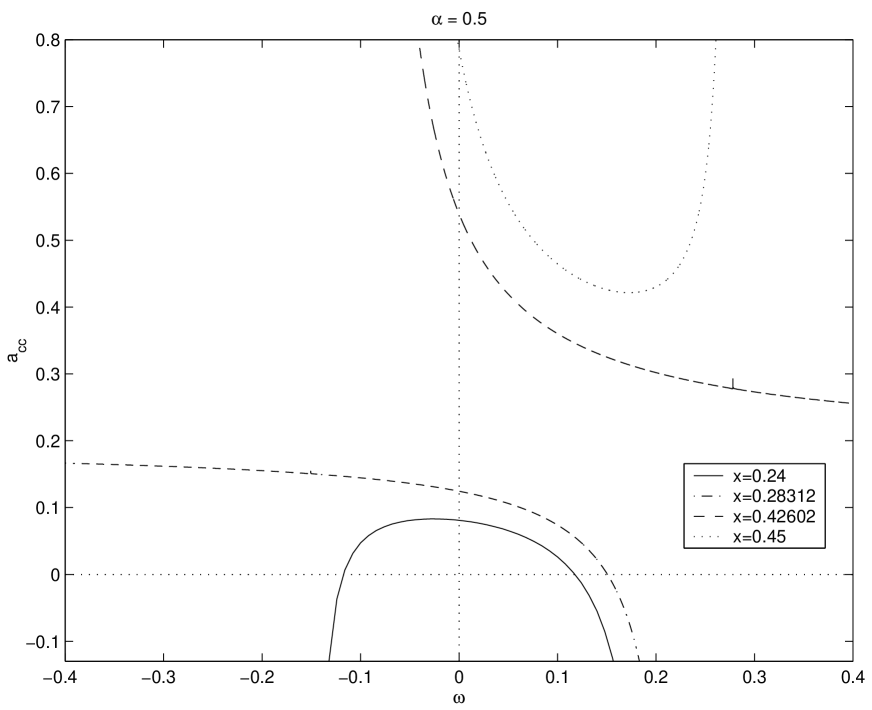
Figure 1: Acceleration required to keep orbits circular as a function of the scaled angular frequency. Plots are shown for different distances from the source, $x\equiv M/r=0.24,0.28312,0.42602,0.45$. The Kerr parameter is $\alpha=0.5$.

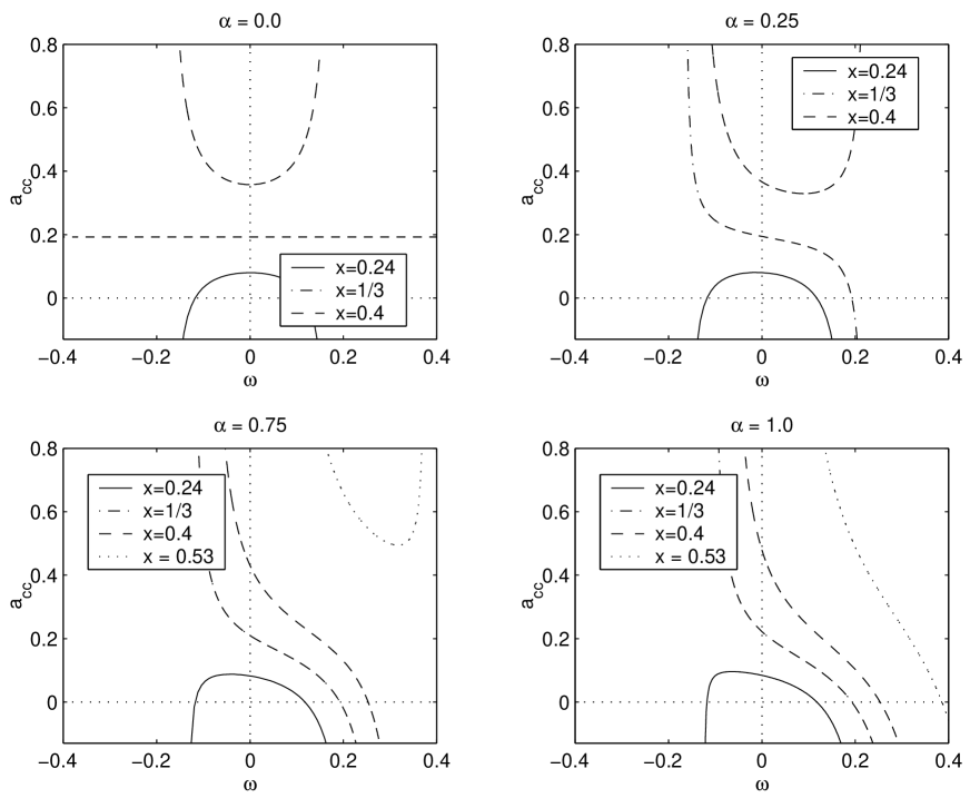
Figure 2: Acceleration required to keep orbits circular as a function of the scaled angular frequency. Plots are shown for different distances from the source, $x\equiv M/r=0.24,0.33,0.4,0.53$. The Kerr parameter is $\alpha=0,0.25,0.75,1.0$.

Until now we have focused on determining the acceleration required to keep orbits circular for a range of angular velocities. Suppose we invert the problem and determine angular velocity for known accelerations. To do this we rearrange equation (7),

$$\omega_{\pm}(x;a_{acc})={x\over\chi-1}\left[-\alpha x\pm\sqrt{\alpha^{2}x^{2}+(\chi-1)(-1+2x+\chi x)}\right]$$ (8)

where $\chi\equiv x\Lambda^{1/2}/a_{cc}$.

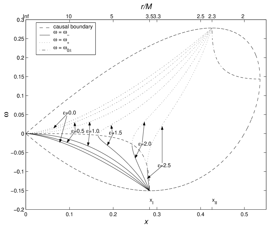
Figure 3: Angular velocity versus distance for $a_{cc}=\epsilon x^{2}\sqrt{\Lambda}/M$ at $\epsilon=0.5,1,1.5,2.0,2.5$ with $\alpha=0.5$.

Figure 3 shows the angular velocity of circular orbits as a function of $x$ for $a_{cc}=\epsilon x^{2}\sqrt{\Lambda}$ at various values of $\epsilon$. The reasons for this choice of acceleration field will become clear later. The permitted angular velocities ($\omega_{c-}<\omega<\omega_{c+}$), correspond to time-like orbits. The solid branch of each curve corresponds to the $\omega_{-}$ solution of (8), the dotted branch to $\omega_{+}$. The family of extremal accelerated circular orbits are shown by the curves $\omega=\omega_{0_{\pm}}$ (to be introduced shortly). Those with $\omega=\omega_{0_{+}}<0$ are maximally accelerated while those with $\omega=\omega_{0_{-}}>0$ are minimally accelerated. The maximum (minimum) acceleration occur for $x<x_{I}$ ($x>x_{II}$), at $\omega=\omega_{0+}$ ($\omega=\omega_{0-}$) where

$$\omega_{0\pm}=-{1\over 2\alpha}\left[1-3x\mp\sqrt{(1-3x)^{2}-4\alpha^{2}x^{3}}\right].$$ (9)

Which correspond to an acceleration

$$a_{0_{\pm}}\equiv a_{cc}(\omega_{0_{\pm}})={x\Lambda^{1/2}\over M}{\sqrt{(1-3x)^{2}-4\alpha^{2}x^{3}}\mp(1-3x)\over\sqrt{(1-3x)^{2}-4\alpha^{2}x^{3}}\mp(1-3x+2\alpha^{2}x^{2})}.$$ (10)

With the exception of the static limit ($\alpha=0$), $\omega_{0\pm}\neq 0$ for all $x>0$. The real zeros of the argument of the square-root, specify $x_{I}$ and $x_{II}$. Figure 4 is a plot of $x_{I}$ and $x_{II}$ versus $\alpha$. It can be shown analytically, or seen from figure 4 that in the Schwarzschild limit ($\alpha=0$) $x_{I}$ and $x_{II}$ occur at the same distance, $x_{I}=x_{II}=1/3$. As $\alpha$ decreases $x_{I}$ ($r_{I}$ increases) and $x_{II}$ increases ($r_{II}$ decreases) until $\alpha=1$ at which point $x_{I}=1/4$ and $x_{II}=1$.

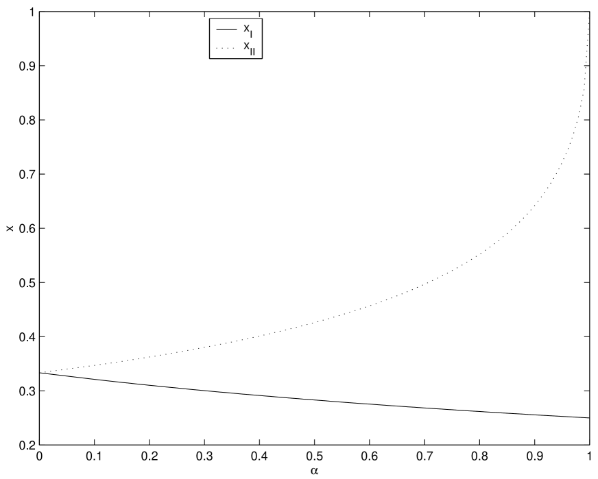
Figure 4: Region boundaries as a function of $\alpha$

3 Non-Keplerian rings

In this section we show that, under certain conditions, stable rings of matter form about compact stellar objects. If the acceleration is sufficiently small, these rings extend quite far from the source and are reminiscent of what would have been a Keplerian disk in the absence of acceleration. For larger accelerations, the rings occur closer to the surface of the star and are more energetic. This last property is related to the effect of the extremal acceleration being at values of $\omega$ less than zero. To see why it is necessary to study the energy equations first.

The time-like covariant component of the four-velocity, $u_{t}$, describes the rest, kinetic, and gravitational energies per unit mass. Assuming that the acceleration field, needed to hold non-geodesic circular orbits, is due to a vector potential $\Phi_{\rho}$, the corresponding potential energy is calculated by solving Hamilton’s equations [17, 18]:

$$\frac{dx^{\rho}}{d\tau}=\frac{\partial{\cal H}}{\partial\pi_{\rho}}$$ (11)

$$\frac{d\pi_{\rho}}{d\tau}=-\frac{\partial{\cal H}}{\partial x^{\rho}},$$ (12)

where ${\cal H}$ is the super-Hamiltonian, $x^{\alpha}$ is a general coordinate (not be confused with the radial parameter $x$ introduced in (6)) and $\pi_{\rho}$ is the momentum conjugate to $x^{\rho}$. The super-Hamiltonian for a minimally coupled vector potential $\Phi_{\rho}$, is:

$${\cal H}={1\over 2m}(\pi_{\rho}-\Phi_{\rho})(\pi^{\rho}-\Phi^{\rho}).$$ (13)

Let the potential be described by a stationary, spherically symmetric scalar field in a Kerr space-time, with:

$$\Phi_{\rho}=-V(r)\delta^{t}_{\rho}+\alpha V(r)\delta^{\phi}_{\rho}$$ (14)

where $V(r)$ is a real, differentiable, scalar function, depending on the radial coordinate only since we require stationarity and axial symmetry, and we confine our attention to the equatorial plane. In this case, Hamilton’s equations (11) and (12), lead to:

$$mu_{t} = \pi_{t}+V$$ (15)

$$mu_{k} = \pi_{k}+\Phi_{k};\qquad(k=r,\,\theta,\,\phi)$$ (16)

$$\pi_{t} = {\rm constant}\equiv-E$$ (17)

$${\dot{u}_{r}} = -u^{t}V_{,r}(1-a\Omega)$$ (18)

$$\pi_{\theta} = {\rm constant}=0\quad{\rm for\,\,equatorial\,\,motion}$$ (19)

$$\pi_{\phi} = {\rm constant}\equiv m\lambda.$$ (20)

Here $m$ is the rest mass of the particle, $E$ and $\lambda$ are its total energy and specific azimuthal angular momentum respectively. If the strength $a_{cc}$ of the acceleration field is known, then the corresponding scaled angular velocity $\omega$ can be determined from equation (8). Written in terms of the parameters $x,\,\alpha,\,\omega$ as in equation (6), equation (18) becomes:

$$x^{3}V(x)_{,x}=mMa_{cc}(\omega_{c_{+}}-\omega)^{1/2}(\omega-\omega_{c_{-}})^{1/2}\Lambda^{-1/2}.$$ (21)

For any fixed value of $\omega$, the potential energy $V$ is calculated by integrating equation (21) provided that the acceleration field and a boundary condition are known. The exact form of the acceleration field will depend on interaction of the photon field with the surrounding matter and of that matter with itself. It is not necessary for us to go into such complexity, for as we shall see, the exact form of the acceleration field is not crucial to the results. We shall side-step the whole issue of determining the acceleration field and simply choose it to be the following:

$$a_{cc}=\frac{\epsilon x^{2}\sqrt{\Lambda}}{M}.$$ (22)

The reasons for choosing this form of acceleration field are that, it is simple, the Newtonian limit is an inverse square law, and it simplifies the integration of equation (21). The $\sqrt{\Lambda}$ term in equation (22) can be thought of as due to gravitational red-shift.

Figure 5 shows the numerical integration of equation (21) for a unit mass in an acceleration field described by equation (22) with the boundary condition $V(0)=0$. From this figure we see that the potential energy $V$ levels off at $x_{I}$ for $\omega_{-}$ orbits and $x_{II}$ for $\omega_{+}$ orbits.

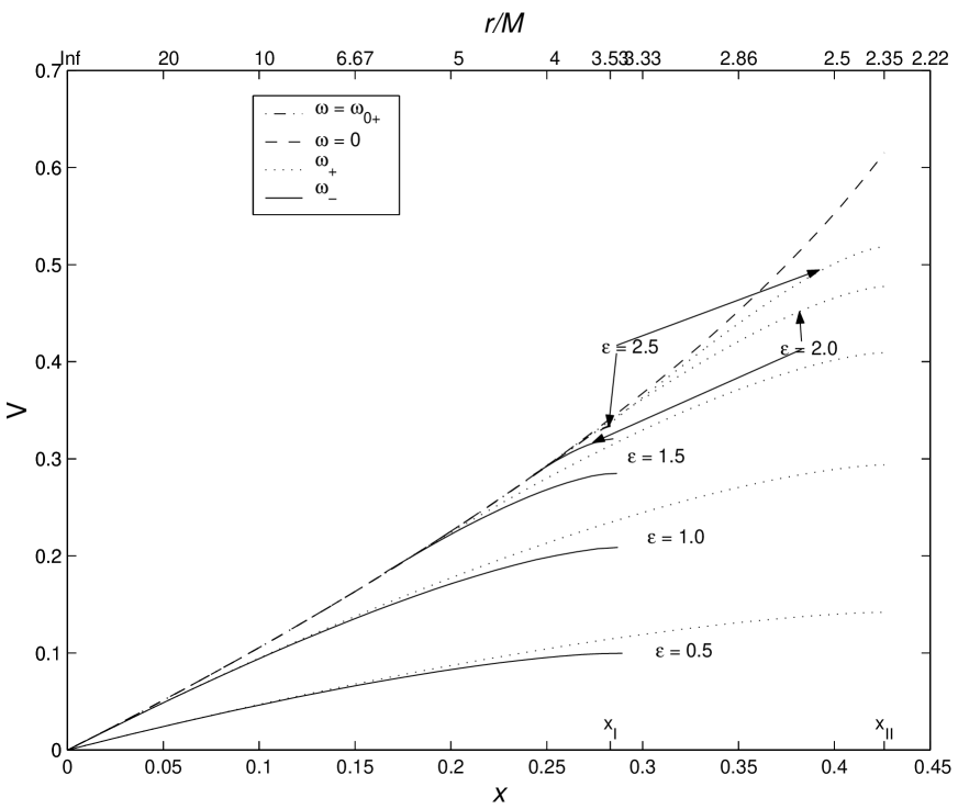
Figure 5: The potential energy as a function of distance for the acceleration field described by (21) for $\epsilon=0.5,1.0,1.5,2.0,2.5$.

The total energy $E$ comprises of both, the potential energy $V$ and the specific energy $mu_{t}$. The specific energy is calculated from (1) and (2),

$$-u_{t}={x+\alpha x\omega-2x^{2}\over\sqrt{x^{2}-2x^{3}+2\alpha x^{2}\omega-\omega^{2}}}\equiv\gamma.$$ (23)

Figure 6 shows the specific energy for the acceleration field given in equation (22).

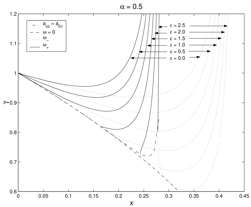
Figure 6: Specific energy as a function of $x\equiv M/r$ in an acceleration field given by equation (22) for $\alpha=0.5$.

It has been known for quite some time that both stable counter-rotating and co-rotating geodesics have a minimum energy [19]. The location of this minimum marks the corresponding last stable orbit, as circular orbits below this limit require a larger energy.

The location of the minimum is determined by solving $\frac{d\gamma}{dx}=0$ for $\omega=\pm x^{3/2}$. In the presence of an acceleration field a minimum in energy can still occur, but it is located at $\frac{dE}{dx}=0$, where $E$ is the sum of the specific and the potential energies, $E=m\gamma+V$. The location and value of the minimum of the energy can be determined using equations (21)–(23), though in general it is a rather messy operation. Since the orbits are not geodesics, the concept of stability here should be handled with care; we mean that a small loss of the total energy allows the particle to move on a nearby circular orbit with the same acceleration field. The behaviour of the particles with respect to a small perturbation of the acceleration field itself, is matter of a detailed investigation. Figure 7 shows energy per unit mass as a function of $x$ for different acceleration fields. We see from these graphs that for sufficiently large acceleration the $\omega_{+}$ orbits have a minimum energy significantly smaller than the energy of the outer orbit. The reason for this is that while the potential energy increases with $x$ the specific energy of the $\omega_{+}$ orbits drop rapidly before increasing again. The sudden drop in the specific energy is due to the sensitivity of the kinetic energy to changes in the modulus of $\omega$. Figure 3 shows that $\omega_{+}$ changes from negative to zero in a comparatively small region before becoming positive. For large accelerations $\omega_{+}$ at the outer boundary is close to the causal limit hence the kinetic energy is large. This kinetic energy drops to a minimum as $\omega_{+}$ approaches zero and then increases as $\omega_{+}$ increases. The potential energy on the other hand does not change significantly and hence a minimum energy occurs when $\omega_{+}\approx 0$.

In the presence of an outward pointing acceleration field, there exists, in general, both an inner and an outer boundary. The inner boundary is determined by the minimum in the energy. An outer boundary occurs if, at some point, the acceleration field is greater than the maximal acceleration, since circular orbits exist in region 1 if and only if $a_{cc}\leq a_{0_{+}}$. The Mac Lauren expansion of equations (10) and (22) both vanish at infinity, namely at $x=0$. However, for $\epsilon>1$ the maximal acceleration $a_{0+}$ vanishes more quickly, hence, for any given value of $\epsilon>1$, there are no circular orbits sufficiently far from the source. As $x$ increases, so does $a_{0+}$. The point where $a_{cc}=a_{0+}$, is the outer radius, $x_{o}$ say, as it is the smallest value of $x$ (the largest value of $r$) where a circular orbit is allowed.

If both inner and outer boundaries exist then a ring structure is formed.

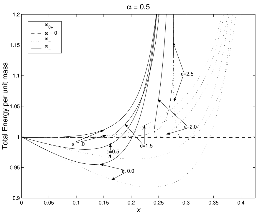
Figure 7: Total energy as a function distance $x\equiv M/r$ of circular orbits in the equatorial plane of a Kerr space-time with $\alpha=0.5$ and an acceleration field given by equation (22). Plots are for $\epsilon=0.0,0.5,1.0,1.5,2.0$, and 2.5.

The efficiency of energy emitted is calculated by comparing the energy of the outer orbit with the inner one, i.e.,

$${\rm energy\>efficeincy\>}=\frac{E(x_{o})-E(x_{i})}{E(x_{o})}$$

For $\epsilon=2.5$ the energy efficiency is $11\%$. As $\epsilon$ increases so does the efficiency until $a_{cc}(x_{I})=a_{0+}(x_{I})$, at which point $E(x_{o})=E(x_{I})=0$.

4 Astrophysical Implications

The ring structures carry a large amount of energy which can be converted into heat and radiation if accretion takes place. The amount of energy which can be released, is given by the difference between the total energies of the outer and the inner boundaries.

The counter-rotating rings carry an amount of energy which increases with $\epsilon$ as shown in figure 7. It is possible to compare the energy output, in the case of accretion, from any given non-Keplerian ring of matter, with that of a Keplerian disk. For the latter case the outer boundary, with $E_{out}=1$, is at infinity, while the inner boundary is at $x\approx 0.283$ with $E_{in}\approx 0.917$, for $\alpha=0.5$, implying only an $8\%$ efficiency. Although in our case it is not appropriate to talk about efficiency, since the energy needed to first generate the acceleration field and set up the ring pattern is not known, we may just consider the efficiency of the energy release of a given ring by accretion, say, only once it was formed.

As it is clearly shown by figure 7, the inner rings can carry a large amount of energy which, once released, can contribute significantly to the total energy output of the source. Figure 4 implies that as the star’s rotation increases, these energetic rings extend outward becoming potentially easier to observe. Indeed the effect we are discussing is sensitive to the rotation parameter $\alpha$.

The space outside a radiating source is filled with photons. In this case, the stress energy tensor of dust (non interacting matter) in the presence of a photon field is

$$T_{\alpha\beta}=\rho_{d}u_{\alpha}u_{\beta}+P_{p}g_{\alpha\beta},$$ (24)

where $u^{\alpha}$ is the four velocity of the dust, $\rho_{d}$ is its density and $P_{p}$ is the photon pressure. By contracting the conservation equation ($T^{\beta}_{\gamma};_{\beta}=0$) with the projection tensor $h_{\alpha}^{\gamma}=\delta_{\alpha}^{\gamma}+u_{\alpha}u^{\gamma}$, the acceleration can be expressed in terms of the pressure gradient [20]. If the four velocity is given by equation (2), then

$$\dot{u}_{\alpha}=-{\partial_{\alpha}P_{p}\over\rho_{d}}.$$

From metric (1) and assuming that the radiation pressure is only radial, then

$$a_{cc}={\Lambda^{1/2}|\partial_{r}P_{p}|\over\rho_{d}}.$$ (25)

5 Conclusions

In this paper, we have shown that highly energetic rings of matter can occur around the exterior of compact stars. We have shown that these rings can achieve energy efficiencies much greater than those of Keplerian disks. We have also shown that the size and energy efficiency of these rings depends on, the specific angular momentum of the star, its mass, the strength of the acceleration field it produces, and the properties of the matter with the ring itself.

This paper forms the corner stone of work to come. Having established the general theory behind the formation of non-Keplerian rings there is still a lot of theoretical and modelling work to be done. For example, the results of this work make it possible to determine the energy efficiency as a function of angular velocity for a given acceleration field. Once this has been done it is then possible to deduce the spin rate of a star from the amount of energy produced by its rings.

The acceleration field we have studied in this paper is only one of many possibilities. While the general property of the formation of rings is not likely to change for different models of the acceleration the specific nature of the rings, such as their size and efficiency will.

The structure of matter within the rings will determine the acceleration field there. It would be interesting to examine the fields produced by matter with a polytropic equation of state.

Similarly, the Hamiltonian describing the particle dynamics was chosen to be a minimally coupled one, but there are many other options. Even the choice of vector potential is not unique and more theoretical work is needed to understand the form it should take.

The possibilities for extensions of this work, while not endless are certainly large. The consequences of such work are that it will make it possible to determine some of the fundamental properties of the stars by observing the rings around them.

Acknowledgments

This work was supported by the Ministero degli Affari Esteri e dal Ministero della Ricerca Scientifica e Tecnologica of Italy. I wish to thank the Director of the Department of Physics G. Galilei of the University of Padova for his hospitality during my stay. I would also like to thank Fernando de Felice for many helpful discussions and good advice.

References

- [1] Burderi L. King A. R. and Szuszkiewicz E. 1998 ApJ. 509 85
- [2] King A. R. 1998 MNRAS 296 L45
- [3] Weinberg S. 1972 Gravitation and Cosmology (New York:John Wiley & Sons)
- [4] Chandrasekhar S. 1983 The Mathematical Theory of Black Holes (New York: Oxford Univ. Press)
- [5] Krasinski A. 1978 Ann. Phys. 112 22
- [6] McManus D. 1991 Class. Quantum Grav. 8 863
- [7] Magli G. 1993 Gen. Rel. & Grav. 25 1277
- [8] Magli G. 1995 J. Math. Phys. 36 5877
- [9] Drake S. P. and Turolla R. 1997 Class. Quantum Grav. 14 1883
- [10] Abramowicz M. A. and Lasota J-P 1974 Acta Phys. Pol. B 5 327
- [11] de Felice F. and Usseglio-Tomasset S. 1991 Class. Quantum Grav. 8 1871
- [12] de Felice F. 1994 Class. Quantum Grav. 11 1283
- [13] de Felice F. 1995 Class. Quantum Grav. 12 1119
- [14] Wald R. M. 1984 General Relativity (Chicago: The University of Chicago Press)
- [15] Geroch R. P. and Horowitz G. T. 1979 “Global Structures of Spacetimes” General Relativity, an Einstein Centenary Survey, ed. S. W. Hawking and W. Israel (Cambridge: Cambridge University Press)
- [16] Penrose R. 1979 “Global Structures of Spacetimes”General Relativity, an Einstein Centenary Survey, ed. S. W. Hawking and W. Israel (Cambridge: Cambridge University Press)
- [17] Jackson J. D. 1975 Classical Electrodynamics (2nd Ed.) (New York: John Wiley & Sons Inc.)
- [18] Goldstein H. 1980 Classical Mechanics (Reading: Addison-Wesly)
- [19] de Felice F. 1968 Il Nuovo Cimento 57B 351
- [20] Stephani H. 1982 General Relativity (Cambridge: Cambridge University Press)