The Numerical Evolution
of
Neutron Star Oscillations
Dissertation
zur Erlangung des Grades eines
Doktors der Naturwissenschaften
der Fakultät für Physik
der Eberhard-Karls-Universität zu Tübingen
vorgelegt von
Johannes O. Ruoff
aus Sindelfingen
2000

Tag der mündlichen Prüfung:	28. 2. 2000
Dekan:	Prof. Dr. Klaus Werner
1. Berichterstatter:	Prof. Dr. Hanns Ruder
2. Berichterstatter:	Prof. Dr. Pablo Laguna

Abstract

The present work investigates the numerical evolution of linearized oscillations of non-rotating, spherically symmetric neutron stars within the framework of general relativity.

We derive the appropriate equations using the (3+1)-formalism. We first focus on the evolution of radial oscillations, which do not emit gravitational waves. The associated system of equations being quite simple, we demonstrate how to handle a numerical instability that also occurs in the non-radial case, when the stellar model is constructed based on a realistic equation of state. We devise a coordinate transformation that not only removes this instability but also provides much more accurate results. For comparison reasons, we compute the eigenfrequencies of the radial modes with an eigenvalue code and thereby confirm the results of Väth & Chanmugam, which differ from previous calculations that were performed by Glass & Lindblom.

The main part deals with the evolution of non-radial oscillations ($l\geq 2$) of neutron stars. Here, we compare different formulations of the equations and discuss how they have to be numerically dealt with in order to avoid instabilities at the origin. We present results for various polytropic stellar models and different initial data. They show that the quasi-normal modes of the star, such as the $f$-, the $p$-, and the $w$-modes, can, indeed, be excited by suitable initial data. However, the excitation strength of the $w$-modes strongly depends on the chosen initial data. For some initial data the occurrence of the $w$-modes can be totally suppressed.

For ultra-compact models we find the interesting feature that the first ring-down phase of the wave signal cannot be associated with any of the known quasi-normal modes that belong to the star itself; the frequency and damping time rather correspond to the first quasi-normal mode of an equal mass black hole.

When switching to realistic equations of state, we find that we face the same numerical problems as in the radial case. Here, too, we can get rid of them by means of the same coordinate transformation inside the star, but things are more complicated because the fluid equation is coupled to the metric equations, which propagate the gravitational waves. For those equations the transformation is not defined, therefore we have to interpolate between the different grids. For polytropic equations of state this can give rise to a quite strong violation of the Hamiltonian constraint, which can spoil the resulting wave signal. However, for realistic equations of state, and it is only for those that the transformation is necessary, this does not happen and the equations can be integrated in a stable way and also provide quite accurate results.

In the last part of this thesis we consider a physical mechanism for exciting oscillations of neutron stars. We use the time dependent gravitational field of a small point mass $\mu$ that orbits the neutron star to induce stellar oscillations. Hereby, we assume $\mu$ to be much smaller than the mass $M$ of the neutron star. In this so-called particle limit, the gravitational field of the moving particle is considered to be a perturbation of the background field of the neutron star. With this particle we have a physical means which removes the arbitrariness in choosing the initial data.

However, even with the presence of the particle, there is still too much freedom in constructing the initial data, which is due to the fact that in addition to the field of the particle we always can superpose any arbitrary amount of gravitational waves. Our task is to minimize this additional gravitational-wave content and find initial data which correspond to the pure gravitational field of the particle. By looking at the flat space case we can construct analytic initial data that satisfy the above requirements. Those then will serve as a good approximation for the “real” initial data in the curved spacetime of the neutron star. By sampling various orbital parameters of the particle we show that in general the particle is not able to excite any $w$-modes. It is only for speeds very close to the speed of light that the $w$-mode is a significant part of the wave signal. This result indicates that it is rather improbable that any physical mechanism which can be simulated by an orbiting particle can excite the $w$-modes of neutron stars in a significant manner.

Chapter 1 Introduction

The investigation of stellar oscillations has a quite long history, and is a whole astrophysical branch on its own. The evaluation of the oscillation modes of stellar objects has helped to reveal a lot of information about their interior structure. With the use of asteroseismological methods we now have a quite detailed understanding of the physics of a whole range of stellar objects, be it our own sun or a white dwarf somewhere in our galaxy.

Most stellar objects can be adequately described by Newtonian theory, however, for very compact objects such as neutron stars, the effects of general relativity cannot be longer neglected. In fact, they are very important, for now, stellar oscillations will be associated with the emission of gravitational waves, which can carry important information about the physics inside those compact objects. These waves, when detected, will open a totally new observational window for astrophysicists. Gravitational waves are not affected by events at the surface of the star, which is what happens to electromagnetic radiation and they also remain practically unaffected by any kind of matter while travelling through space. Thus, they carry “clean” information of the physical properties of the neutron stars.

It is well known that lowest gravitational-wave multipole is the quadrupole radiation, hence the radial and dipole oscillations do not emit gravitational waves. From the gravitational-wave astronomical point the latter are therefore quite uninteresting, however, they could make themselves visible through tiny undulations in the electromagnetic radiation signal of the neutron stars.

The study of the non-radial oscillations modes of non-rotating neutron stars within the framework of general relativity was initiated in 1967 by a series of papers by Thorne and several coauthors [18, 19, 20, 21, 22]. In the following decades a lot of authors made endeavors to study the relativistic oscillation spectrum of neutron stars, which turned out to be particularly rich.

From the general Newtonian theory of non-radial linear oscillations it follows that the oscillations of a spherical stellar object can be divided into two classes according to their transformation behavior under space reflection. One class consists of even parity or polar modes; the odd parity or axial modes belong to the other class.

If the neutron star is modeled with a perfect fluid then from Newtonian theory it follows that any non-radial oscillations such as the $f$undamental mode [30], the $p$ressure modes, and the $g$ravitational modes [34], must belong to the polar class. This means that for Newtonian perfect fluid stellar models there are no axial modes at all. It is only with the inclusion of a solid crust that there can exist axial $t$orsional modes.

In the first 20 years after the fundamental paper of Thorne, it was common belief that the oscillation spectra of relativistic neutron stars would not differ much from Newtonian stars. The only new effect of general relativity was thought to be the radiation-damping of the oscillation modes due to the emission of gravitational waves. Therefore the main focus was to compute the frequencies and damping times of those polar modes which also exist in the Newtonian theory, but now within the framework of general relativity. The only axial modes under consideration were the $t$-modes of neutron stars with a solid crust [32, 35, 40].

It was only in 1988 that another family of polar modes was found by Kojima [38], whose existence has already been anticipated two years earlier in a toy model by Kokkotas & Schutz [36]. Those new modes, which were termed $w$ave-modes by Kokkotas & Schutz [45], are of purely relativistic origin and do not have a Newtonian counterpart. They are predominantly metric oscillations and couple only weakly to the motion of the matter.

Around the same time Chandrasekhar & Ferrari [42] showed that for ultra-relativistic stellar models, there exists also a family of axial perturbations, which do not couple to the matter at all. This is because the spacetime curvature inside the star can be so strong that it can trap impinging gravitational waves. Those “trapped” modes are quite long-lived since they correspond to quasi-bound states inside the gravitational potential of the neutron star, which only slowly leak out.

A little later, it was found by Leins et al. [48] that the polar $w$-modes are split into two branches, one with only a few strongly damped modes (called $w_{II}$- or interface modes), and the other one with an infinite number of modes with increasing frequency and damping times.

In 1994 Kokkotas [50] showed that for less relativistic stars, which do not possess any trapped modes, there also exists a family of axial modes, which are quite similar to the polar $w$-modes. Finally, in 1996 Andersson et al. [51, 52] established that all three kinds of gravitational-wave modes (the $w$-modes, the $w_{II}$-modes and the trapped modes) exist for both the polar and the axial cases, the trapped modes, however, only for ultra-relativistic star.

This rich set of various pulsation modes having been found, it then was natural to ask whether they would indeed be excited in a real pulsation scenario. Allen et al. [54] took a first step in answering this question by numerically integrating the evolution equations for several different sets of initial data. By looking at the emitted gravitational radiation, they indeed found that both the fluid $f$- and $p$-modes and the gravitational $w$-modes can be excited. However, the excitation strength depends strongly on the choice of initial data, which, of course, were constructed ad hoc and had no astrophysical meaning whatsoever.

Andersson & Kokkotas [55] have shown that, once the parameters of the $f$- and the first $w$-mode are known, it is in principle possible to obtain the mass and the radius of a neutron star quite accurately. Those quantities could then be used to determine the equation of state for the neutron star matter. Because of the still quite poor understanding of the physics at the subnuclear density level, there exists a plethora of different equations of state in the literature, all based on different physical models of the nuclear interaction. But once the mass and radius of a neutron star are known with a certain accuracy, it is possible to rule out those equations of state that predict a different radius for a given mass, or vice versa. And this in turn would hint at the physics that governs the behavior of the neutron star matter in the center of the star.

It is therefore of particular interest whether or not the $w$-modes will be excited in a real astrophysical scenario such as the collapse of a progenitor star to a neutron star. Whereas the $f$- and some fluid $p$-modes will always be present in an wave signal, it is not clear if this is also the case for the $w$-modes. The numerical experiments show that it is possible to construct initial data which do not excite any $w$-modes at all.

To satisfactorily answer the question what a real signal would look like, one would have to follow the appropriate scenario (e.g. the collapse of a burned out star core) in full detail from the point on where relativistic effects become important. Unfortunately, this is, for the time being, still impossible. This is mainly because one would have to use the full set of the nonlinear Einstein equations together with the whole machinery of nuclear physics to simulate a core collapse. However, when the newborn neutron star has almost settled, the study of stellar pulsations can be done within the linearized theory, which makes it tractable. But even there one usually restricts oneself to very simple neutron star models. In our case, we will neglect the spin of the star, which makes the equations much simpler, but also prevents us from studying the effects of rotation, which might be very important.

There are no unstable non-radial modes for non-rotating stars as long as the Schwarzschild discriminant

$$S(r)\; =\;\frac{dp}{dr}-\left(\frac{\partial{p}}{\partial{\epsilon}}\right)_{s}\frac{d\epsilon}{dr}$$

is positive [27, 71]. For negative $S$ the oscillations become unstable with respect to convection. In this thesis we always use barotropic equations of state, for which it is $S\equiv 0$, therefore all non-radial modes will be stable.

However, things can change dramatically when rotation is included. There will be always some modes which will undergo the CFS-instability [68, 69, 70], and recently a whole set of unstable modes ($r$-modes) has been discovered. They might be responsible for slowing down rapidly rotating neutron stars [56]. For a recent review of the stability properties of rotating neutron stars, see [72]. Other recent reviews on oscillations of neutron stars and black holes can be found in [59, 60].

The thesis is organized as follows:

In chapter 2 we will derive the general form of the perturbation equations using the (3+1)-split.

In chapter 3 we will specialize on the radial case, where we investigate both the evolution and the eigenvalue problem. We discuss the occurrence of a numerical instability, which occurs both in the radial and non-radial cases when the neutron star is modeled with a realistic equation of state. We also present a remedy which not only removes the instability but also automatically increases the accuracy of the evolution as compared to the old set of equations.

In chapter 4 we focus on the non-radial oscillations. We present various forms of the equations and discuss which of them are the most suitable set for the numerical evolution. We show how to treat the boundary conditions in order to obtain stable evolutions for any value of $l$. Here, too, we demonstrate how to get rid of the same numerical instability that occurs with the use of realistic equations of state.

In chapter 5 we examine the excitation of neutron star oscillations by the scattering of a small point mass $\mu$ in the particle limit, where we assume $\mu$ to be much smaller than the mass $M$ of the neutron star. The gravitational field of the particle, which follows a geodesic path in the background metric of the neutron star, can then be treated as a perturbation of the background. We sample a variety of orbital parameters to see whether or not the particle is able to excite the $w$-modes of the neutron star.

Notations and conventions

• We use Einstein’s sum convention. Greek indices run from 0 to 3, Latin indices from 1 to 3. The time component is the 0-component.

• The signature of the metric is $(-,+,+,+)$, i.e. time-like 4-vectors have negative norm.

• We use geometric units, i.e. we set $c=G=1$.

• Covariant derivatives with respect to $x^{\mu}$ are denoted by $D_{\mu}$ and partial derivatives $\frac{\partial{}}{\partial{x^{\mu}}}$ are sometimes abbreviated by $\partial_{\mu}$.

• Derivatives with respect to the radial coordinate $r$ are often denoted by a prime, and time derivatives by an over-dot.

• The perturbation variables should be properly denoted by $Q_{lm}(t,r)$, however, we will often omit the indices $l$ and $m$.

Chapter 2 Linearizing Einstein’s equations

Within perturbation theory we first construct a stationary non-pulsating and non-rotating neutron star model by solving Einstein’s equations, which in this case reduce to a set of coupled ordinary differential equations.

Having found this (numerically) exact background solution $g_{\mu\nu}$, we describe the pulsations by “small” deviations from the original metric. Thus, the metric of the perturbed spacetime will be written as $\bar{g}_{\mu\nu}=g_{\mu\nu}+h_{\mu\nu}$, where $h_{\mu\nu}$ is considered to be a small perturbation of the background metric $g_{\mu\nu}$.

To find the relevant equations for $h_{\mu\nu}$, we plug the perturbed metric $\bar{g}_{\mu\nu}$ into Einstein’s equations and neglect all terms that are quadratic or of a higher power in the $h_{\mu\nu}$. We will thus obtain a linear system of partial differential equations for the $h_{\mu\nu}$, which is much easier to solve than the full nonlinear set. Still, this set of equations depends on all four coordinates, which, even with the presently available computer power, would be too time-consuming to be solved in its fullfledged form.

However, because of the spherical symmetry of the background metric we can get rid of the angular dependence by expanding the perturbation equations into spherical tensor harmonics. It is thus possible to reduce the equations into a (1+1)-dimensional evolution system, which can be numerically solved on present day PCs.

2.1 The unperturbed stellar model

The simplest model for a neutron star is a non-rotating zero temperature perfect fluid sphere, whose static spherically symmetric geometry is given by a line element of the form

$$ds^{2}\; =\;-e^{2\nu}dt^{2}+e^{2\lambda}dr^{2}+r^{2}(d\theta^{2}+\sin^{2}\theta d\phi^{2})\;,$$ (2.1)

where the two functions $\nu$ and $\lambda$ only depend on the radial coordinate $r$ and have to be determined by the field equations. The appropriate energy-momentum tensor is given by

$$T_{\mu\nu}\; =\;\left(\epsilon+p\right)u_{\mu}u_{\nu}+pg_{\mu\nu}\;,$$ (2.2)

where $p$ is the pressure, $\epsilon$ the energy density, and $u_{\mu}$ the covariant 4-velocity of the fluid. In the rest frame of the fluid, which is static, the only non-vanishing component is the time component $u_{0}=-e^{\nu}$, and Einstein’s equations $G_{\mu\nu}=8\pi T_{\mu\nu}$ and the conservation equations $D_{\nu}T^{\mu\nu}=0$ yield the following three structure equations for the four unknown $\lambda,\,\nu,\,p$, and $\epsilon$:

$$\lambda^{\prime}\; =\;\frac{1-e^{2\lambda}}{2r}+4\pi re^{2\lambda}\epsilon$$ (2.3a)

$$\nu^{\prime}\; =\;\frac{e^{2\lambda}-1}{2r}+4\pi re^{2\lambda}p$$ (2.3b)

$$p^{\prime}\; =\;-\nu^{\prime}(p+\epsilon)\;.$$ (2.3c)

To fully determine this system of equations, an equation of state

$$p\; =\;p(s,n)$$ (2.4)

$$\epsilon\; =\;\epsilon(s,n)$$ (2.5)

must be supplemented. We will refer to the equations (2.3) as Tolman-Oppenheimer-Volkov or TOV equations, even if the original TOV equations are written in a slightly different form.

Throughout this work we always assume the neutron star to have zero temperature, which is quite reasonable since the pressure inside the neutron star is mainly maintained by a Fermi gas of degenerate neutrons. Hence, the specific entropy $s$ can be set to zero, too, and we can eliminate the baryon density $n$ and obtain a barotropic equation of state, where the pressure is a function of the energy density alone:

$$p\; =\;p(\epsilon)\;.$$ (2.6)

The simplest and therefore quite often used form is given by a so-called polytropic equation of state

$$p\; =\;\kappa\epsilon^{\Gamma}\;,$$ (2.7)

where $\kappa$ and $\Gamma$ are the polytropic constant and polytropic index, respectively. More realistic equations of state have to include the microphysics that dictates the interplay between $p$ and $\epsilon$ on the nuclear and subnuclear levels for the neutron star matter. However, the physics under the extreme conditions of the high pressures that prevail in the center of neutron stars is not yet fully understood. In the literature there are therefore quite a few different realistic equations of state, which were calculated based on various different microscopic models of (sub)nuclear interactions.

It is clear that the zero temperature assumption neglects all kinds of thermal and viscous effects which can affect the stellar oscillations. On the one hand it will suppress the existence of the whole family of $g$-modes, and on the other hand we ignore the effects of viscosity and internal friction, which would normally damp out any oscillation. However, the damping times [37] are such that their neglect will have no effect on the numerical evolutions we are investigating.

If we introduce an additional function $m$, which is related to $\lambda$ by

$$e^{-2\lambda}\; \equiv\;1-\frac{2m}{r}\;,$$ (2.8)

we obtain from (2.3a)

$$m^{\prime}\; =\;4\pi r^{2}\epsilon\;.$$ (2.9)

Integration immediately leads to

$$m(r)\; =\;\int^{r}_{0}4\pi{\tilde{r}}^{2}\epsilon\,d\tilde{r}\;,$$ (2.10)

which makes it clear that $m(r)$ represents the total gravitational mass enclosed inside the radius $r$.

To obtain the stellar model, we have to integrate the TOV equations (2.3) together with (2.6) from the center up to the point where the pressure $p$ vanishes. This then defines the surface $R$ of the star.

From Birkhoff theorem it follows that the exterior vacuum region of the star is described by the Schwarzschild metric with the mass parameter $M\equiv m(R)$.

2.2 The perturbation equations

A somewhat more elaborate derivation of the relevant equations can be found in my Diploma thesis [53]. Here, we will only briefly discuss the necessary steps and not go into very great details. Our starting point is the ADM-formulation [73] or (3+1)-decomposition of the Einstein equations. In this formulation the 10 field equations are first split into 6 dynamical equations and 4 constraint equations. The dynamical equations, which have second order time derivatives, are then cast into a set of 12 evolution equations, which are first order in time. Those are the 6 evolution equations for the 3-metric $\gamma_{ij}$ of a space-like 3-dimensional hypersurface $\Sigma$ and another 6 equations for the time development of its extrinsic curvature $K_{ij}$:

$$\partial_{t}\gamma_{ij}\; =\;-2\alpha K_{ij}+\beta^{k}\partial_{k}\gamma_{ij}+\gamma_{ki}\partial_{j}\beta^{k}+\gamma_{kj}\partial_{i}\beta^{k}$$ (2.11)

$$\begin{split}\partial_{t}K_{ij}\;&=\;\alpha\left[R_{ij}+KK_{ij}-2K_{ik}K^{k}_{\phantom{i}j}-8\pi\left(T_{ij}-\frac{1}{2}T\gamma_{ij}\right)\right]\\ &\quad{}-D_{i}D_{j}\alpha+\beta^{k}\partial_{k}K_{ij}+K_{ik}\partial_{j}\beta^{k}+K_{jk}\partial_{i}\beta^{k}\;.\end{split}$$ (2.12)

Herein, $\alpha$ denotes the lapse function and $\beta^{i}$ is the shift vector. The remaining 4 constraint equations, which have to be satisfied by any physically acceptable initial data, are given by

$$R-K_{ij}K^{ij}+K^{2}\; =\;16\pi\rho$$ (2.13)

$$D_{i}K-D_{j}K^{j}_{\phantom{j}i}\; =\;8\pi j_{i}\;.$$ (2.14)

Here, $\rho$ and $j_{i}$ are the energy density and momentum density measured by a momentarily stationary observer, whose 4-velocity coincides with the time-like normal vector $n^{\mu}$ of the space-like hypersurface:

$$\rho\; =\;T_{\mu\nu}n^{\mu}n^{\nu}$$ (2.15)

$$j_{i}\; =\;T_{i\nu}n^{\nu}\;.$$ (2.16)

The scalar equation (2.13) is usually called the Hamiltonian constraint and the vector equation (2.14) is called momentum constraint. Once satisfied on the initial hypersurface, they will be automatically preserved throughout the evolution by virtue of the Bianchi-identities.

As we have already mentioned above, the oscillations of the neutron star will be described within the framework of perturbation theory, i.e. we will treat them as small perturbations around the fixed background which is given by the unperturbed stellar model. Hence, we write the perturbed metric $\bar{g}_{\mu\nu}$ as a sum of the static background $g_{\mu\nu}$ and the time-dependent perturbations $h_{\mu\nu}$:

$$\bar{g}_{\mu\nu}\; =\;g_{\mu\nu}+h_{\mu\nu}\,.$$ (2.17)

Since we are using the (3+1)-decomposition, we have to write down the perturbed metric (2.17) in terms of lapse function, shift vector, and 3-metric. Furthermore, we have to deal with the extrinsic curvature as a dynamical variable. Their respective perturbations will be denoted by $\alpha$, $\beta^{i}$, $h_{ij}$, and $k_{ij}$. For the background metric (2.1), shift and extrinsic curvature vanish and the unperturbed lapse function $A$ is given by

$$A\; =\;\sqrt{-g_{00}}\;=\;e^{\nu}\,.$$ (2.18)

In addition to the metric perturbations, we have to describe the perturbations of the energy-momentum tensor $T_{\mu\nu}$. For a perfect fluid, the only quantities that can be perturbed are energy density $\epsilon$, pressure $p$, and 4-velocity $u_{\mu}$, whose perturbations will be denoted by $\delta\epsilon$, $\delta p$, and $\delta u_{\mu}$, respectively. For a barotropic equation of state, however, $\delta\epsilon$ and $\delta p$ are not independent but are rather related through

$$\delta p\; =\;\frac{dp}{d\epsilon}\,\delta\epsilon\;,$$ (2.19)

where $\frac{dp}{d\epsilon}=:C_{s}^{2}$ is the square of the sound speed $C_{s}$ inside the fluid.

Due to the simple form of (2.1), the evolution equations for the 3-metric and the extrinsic curvature perturbations do not become as messy as they usually do in perturbation theory:

$$\partial_{t}h_{ij}\; =\;\beta^{k}\partial_{k}\gamma_{ij}+\gamma_{ki}\partial_{j}\beta^{k}+\gamma_{kj}\partial_{i}\beta^{k}-2e^{\nu}k_{ij}$$ (2.20)

$$\begin{split}\partial_{t}k_{ij}\;&=\;-\partial_{i}\partial_{j}\alpha+\Gamma^{k}_{\phantom{i}ij}\partial_{k}\alpha+\delta\Gamma^{k}_{\phantom{i}ij}\partial_{k}e^{\nu}+\alpha\left[R_{ij}+4\pi(p-\epsilon)\gamma_{ij}\right]\\ &\quad{}+e^{\nu}\left[\delta R_{ij}+4\pi\left((p-\epsilon)h_{ij}+\delta\epsilon(C_{s}^{2}-1)\gamma_{ij}\right)\right].\end{split}$$ (2.21)

Herein, $\gamma_{ij}$ denotes the spatial part of (2.1), its inverse is $\gamma^{ij}$, and the perturbed Christoffel symbols are defined as

$$\delta\Gamma^{k}_{\phantom{i}ij}\; =\;\frac{1}{2}\gamma^{km}\left(D_{i}h_{mj}+D_{j}h_{mi}-D_{m}h_{ij}\right)$$

$$=\;\frac{1}{2}\gamma^{km}\left(\partial_{i}h_{mj}+\partial_{j}h_{mi}-\partial_{m}h_{ij}-2\Gamma^{l}_{\phantom{i}ij}h_{lm}\right)\;.$$ (2.22)

The perturbed Ricci tensor is given by

$$\delta R_{ij}\; =\;D_{k}\delta\Gamma^{k}_{\phantom{i}ij}-D_{j}\delta\Gamma^{k}_{\phantom{i}ik}$$

$$=\;\partial_{k}\delta\Gamma^{k}_{\phantom{i}ij}-\partial_{j}\delta\Gamma^{k}_{\phantom{i}ik}+\Gamma^{l}_{\phantom{i}ij}\delta\Gamma^{k}_{\phantom{i}lk}+\Gamma^{k}_{\phantom{i}lk}\delta\Gamma^{l}_{\phantom{i}ij}-\Gamma^{l}_{\phantom{i}ik}\delta\Gamma^{k}_{\phantom{i}lj}-\Gamma^{k}_{\phantom{i}lj}\delta\Gamma^{l}_{\phantom{i}ik}\,.$$ (2.23)

To first order in the perturbations, the constraints (2.13) and (2.14) read

$$\gamma^{ij}\delta R_{ij}-h^{ij}R_{ij}\; =\;16\pi\delta\epsilon$$ (2.24)

$$\gamma^{jk}\left(\partial_{i}k_{jk}-\partial_{j}k_{ik}-\Gamma^{l}_{\phantom{i}ik}k_{jl}+\Gamma^{l}_{\phantom{i}jk}k_{il}\right)\; =\;-8\pi(p+\epsilon)\delta u_{i}\,.$$ (2.25)

It is interesting to note that it is possible to eliminate $\delta\epsilon$ in (2.21) by virtue of the Hamiltonian constraint (2.24) and to obtain thus a consistent system of evolution equations for the metric and extrinsic curvature alone. The constraints then can serve to compute the matter perturbations $\delta\epsilon$ and $\delta u_{i}$. In this case we would not have to use the equations of motion for the matter perturbations, which follow from the conservation of energy-momentum $D_{\nu}T^{\mu\nu}$.

Our next step consists of expanding the equations in spherical tensor harmonics. Any symmetric tensor $A_{\mu\nu}$ can be expressed in terms of a set of ten spherical tensor harmonics $\{[{\cal\char 89\relax}^{A}_{lm}]_{\mu\nu}(\theta,\phi)\}_{A=1,...,10}$, namely

$$A_{\mu\nu}(t,r,\theta,\phi)\; =\;\sum_{l=0}^{\infty}\sum_{m=-l}^{l}\sum_{A=1}^{10}a_{A}^{lm}(t,r)\;[{\cal\char 89\relax}^{A}_{lm}]_{\mu\nu}(\theta,\phi)\;.$$ (2.26)

Due to the spherical symmetry of the background we thereby can eliminate the angular dependence and obtain equations for the coefficients $a_{A}^{lm}(t,r)$. The field equations thus will be reduced to partial differential equations in $t$ and $r$.

There are various ways to define those tensor harmonics ${\cal\char 89\relax}^{A}_{lm}$, and an exhaustive overview can be found in [77]. The set first given by Regge and Wheeler [17] is widely used throughout the literature and we will follow this tradition, even if this set has the disadvantage of not being orthonormal. However, this is of no account in the following proceeding. It is only with the inclusion of an orbiting particle that this fact causes some minor inconveniences.

The Regge-Wheeler harmonics can be divided into two subsets that behave in different ways under parity transformation. Under space reflection the polar or even parity harmonics change sign according to $(-1)^{l}$, whereas the axial or odd parity harmonics transform like $(-1)^{l+1}$.

We now expand the metric as follows:

$$\begin{split}h_{\mu\nu}\;&=\;-2e^{\nu}\widehat{S}_{1}^{lm}[{\cal\char 89\relax}^{1}_{lm}]_{\mu\nu}+\widehat{S}_{2}^{lm}[{\cal\char 89\relax}^{2}_{lm}]_{\mu\nu}+\widehat{S}_{3}^{lm}[{\cal\char 89\relax}^{5}_{lm}]_{\mu\nu}\\ &\quad{}+\widehat{V}_{1}^{lm}[{\cal\char 89\relax}^{3}_{lm}]_{\mu\nu}+\widehat{V}_{2}^{lm}[{\cal\char 89\relax}^{4}_{lm}]_{\mu\nu}+\widehat{V}_{3}^{lm}[{\cal\char 89\relax}^{6}_{lm}]_{\mu\nu}+\widehat{V}_{4}^{lm}[{\cal\char 89\relax}^{7}_{lm}]_{\mu\nu}\\ &\quad{}+\widehat{T}_{1}^{lm}[{\cal\char 89\relax}^{8}_{lm}]_{\mu\nu}+\widehat{T}_{2}^{lm}[{\cal\char 89\relax}^{9}_{lm}]_{\mu\nu}+\widehat{T}_{3}^{lm}[{\cal\char 89\relax}^{10}_{lm}]_{\mu\nu}\;.\end{split}$$ (2.27)

The notation has been chosen such that the coefficients $\widehat{S}_{i}$ represent the scalar parts of $h_{\mu\nu}$, namely $\alpha,\beta_{r}$, and $h_{rr}$, whereas the $\widehat{V}_{i}$ stand for the vector components $\beta_{\theta},\beta_{\phi},h_{r\theta}$ and $h_{r\phi}$. Lastly, the $\widehat{T}_{i}$ represent the tensorial components $h_{\theta\theta},h_{\theta\phi}$ and $h_{\phi\phi}$. Note that this expansion includes both polar and axial harmonics. Similarly, the extrinsic curvature tensor $k_{ij}$ will be expanded as

$$\begin{split}k_{ij}\;&=\;\widehat{K}_{1}^{lm}[{\cal\char 89\relax}^{5}_{lm}]_{ij}+\widehat{K}_{2}^{lm}[{\cal\char 89\relax}^{6}_{lm}]_{ij}+\widehat{K}_{3}^{lm}[{\cal\char 89\relax}^{7}_{lm}]_{ij}\\ &\quad{}+\widehat{K}_{4}^{lm}[{\cal\char 89\relax}^{8}_{lm}]_{ij}+\widehat{K}_{5}^{lm}[{\cal\char 89\relax}^{9}_{lm}]_{ij}+\widehat{K}_{6}^{lm}[{\cal\char 89\relax}^{10}_{lm}]_{ij}\;.\end{split}$$ (2.28)

Last not least, we need the matter variables

$$\delta\epsilon\; =\;\hat{\rho}^{lm}Y_{lm}$$ (2.29)

$$u_{i}\; =\;\hat{u}_{1}^{lm}[{\cal\char 89\relax}^{5}_{lm}]_{i1}+\hat{u}_{2}^{lm}[{\cal\char 89\relax}^{6}_{lm}]_{i1}+\hat{u}_{3}^{lm}[{\cal\char 89\relax}^{7}_{lm}]_{i1}\;.$$ (2.30)

Here, $Y_{lm}$ in the expansion (2.29) for $\delta\epsilon$ is just the ordinary spherical harmonic. Using this expansion, we will obtain 12 evolution equations for the coefficients of the 3-metric $h_{ij}$ and the extrinsic curvature $k_{ij}$. However, it is clear that this set cannot be used for the evolution, for we have not specified any gauge yet. Picking a specific gauge means prescribing the coefficients of lapse $\alpha$ and shift $\beta_{i}$ for which we do not have any evolution equations. Of course, there are various ways to choose lapse and shift, and for the numerical evolution of the full nonlinear Einstein equations it is crucial to make a good choice because inadequate lapse or shift may cause the code to crash at very early times due to the blow up of some variables.

However, we are dealing with the linearized field equations and we do not have to worry too much about some of the nasty things that might happen in the nonlinear case. We will choose lapse and shift in a way as to simplify the equations as much as possible.

We could now proceed and write down the general form of the perturbation equations, but we will not do so because on the one hand the equations are quite lengthy and on the other hand they are not very useful as such. Besides, they can be found in Appendix C of my diploma thesis [53]. However, it seems to be appropriate to make some comments on the equations.

First of all, the equations are independent of the spherical harmonic index $m$ because of the spherical symmetry of the background. Secondly, they decouple with respect to their behavior under parity transformation. Hence we obtain two sets of equations, one describing polar perturbations, the other axial ones. The latter cannot generate any density or pressure changes in the neutron star for those quantities are scalars and therefore have even parity. The equations can be further subdivided according to their value of $l$. The radial and dipole modes are characterized by $l=0$ and $l=1$, respectively. Those oscillations do not give rise to gravitational radiation, hence the equations are only meaningful in the interior of the star itself. Of course, they are also valid in the exterior, but we can make them identically vanish by means of an appropriate gauge transformation. Furthermore, for $l=0$ we do not have any angular dependence at all, hence all the metric and extrinsic curvature coefficients that are proportional to a derivative of $Y_{lm}$ vanish identically. We will consider this case in the next chapter. The dipole modes, which have been studied in [25, 31, 39], will not be treated in this thesis.

For $l\geq 2$ it is not possible any more to make the exterior equations vanish, hence those equations describe real gravitational waves, which propagate through the spacetime and carry information about the oscillations of the neutron star. This case is the main point of investigation of this thesis and is presented in chapter 4.

Chapter 3 Radial oscillations of neutron stars

As they are the simplest oscillation modes of neutron stars, radial modes have been the first under investigation [12]. More important, they can give information about the stability of the stellar model under consideration [9, 10]. Since they do not couple to gravitational waves, the appropriate equations are quite simple and it is relatively easy to numerically solve the eigenvalue problem that leads to the discrete set of oscillation frequencies of a neutron star. In the absence of any dissipative processes the oscillation spectrum of a stable stellar model forms a complete set; it is therefore possible to describe any arbitrary periodic radial motion of a neutron star as a superposition of its various eigenmodes. It hence seems quite superfluous to explicitly solve the time dependent equations, for we do not expect to gain new physical insight. This might be true indeed. There are, however, quite unexpected numerical problems that are associated with the evolution of the radial oscillations of realistic neutron star models.

Those problems are quite generic, for they also occur for the non-radial oscillations and probably also in the case of rotating neutron stars, and once we have them under control in the radial case it should be straightforward to confer the appropriate numerical treatment to other cases.

The above mentioned numerical problems are instabilities that occur when the neutron star model is constructed with a realistic equation of state. However, they do not appear, if one uses polytropic equations of state, which is often done for the sake of simplicity. As it turned out, this instability is not a general instability of the numerical scheme, for it is dependent on the resolution and can be made to disappear if the resolution exceeds a certain threshold. However, this threshold strongly depends on the numerical scheme that is used to evolve the equations, and can be so high that it prevents any evolutions within a reasonable time limit. For other discretizations, the threshold can be relatively low and does not represent a real obstacle to obtaining numerical results. However, this is mainly because the radial case is a (1+1)-d problem and one only has to consider the stellar interior, since the exterior spacetime remains totally unaffected. For non-radial oscillations with $l\geq 2$ this is not true any more, for here the oscillations will generate gravitational waves, which propagate towards infinity. This means that we have to include the exterior domain in our numerical evolution as well, which will result in a much bigger computational expenditure. Here, the required minimum resolution can extend the computation time of a single run to quite large values. Still, even the non-radial case is a (1+1)-d problem, and if we include rotation we will face a (2+1)-d problem, which can become totally intractable if a high resolution is required to obtain a stable evolution.

As we shall see, the cause of the instability is confined to a small region close to the surface of the star, and it is only here that the high resolution is needed in order to obtain stability. For the more time-consuming cases, we then could only locally refine the grid in this region instead of using high resolution for the whole domain. However, for each stellar model, we would have to localize the troublesome region and find the required resolution, which is more or less a matter of trial and error.

Therefore, we seek for a better way to solve this problem and we find it in reformulating the equations in such a way that the instability totally disappears, and the equations can be evolved for any stellar model and for any desired resolution in a stable way.

3.1 Derivation of the evolution equations

The first one to write down the equations was Chandrasekhar [9, 10], later on various authors rewrote them in many different ways [11, 13, 14, 16]. Since the (3+1)-formalism is particularly suitable for the numerical evolution we will rederive the equations using the framework of the (3+1)-decomposition.

From the last chapter we know that radial perturbations are described by $l=0$. Since the appropriate harmonic is just a number $Y_{00}=1/\sqrt{4\pi}$ there is no angular dependence at all and any derivative of $Y_{00}$ with respect to $\theta$ or $\phi$ vanishes. In this case we can absorb $Y_{00}$ in the perturbation variables, which are then functions of $t$ and $r$ only, and the expansion of the perturbations reads

$$\alpha\; =\;e^{\nu}S_{1}(t,r)$$ (3.1a)

$$\beta_{r}\; =\;re^{2\lambda}S_{2}(t,r)$$ (3.1b)

$$h_{ij}\; =\;\left(\begin{array}[]{ccc}re^{2\lambda}S_{3}(t,r)&0&0\\ 0&r^{2}T(t,r)&0\\ 0&0&r^{2}\sin^{2}\theta\,T(t,r)\end{array}\right)\;.$$ (3.1f)

Similarly, we have for the extrinsic curvature

$$k_{ij}\; =\;-e^{-\nu}\left(\begin{array}[]{ccc}e^{2\lambda}K_{1}(t,r)&0&0\\ 0&\frac{1}{2}r^{2}K_{2}(t,r)&0\\ 0&0&\frac{1}{2}r^{2}\sin^{2}\theta K_{2}(t,r)\end{array}\right)\;.$$ (3.5)

This particular decomposition has been chosen in order to obtain a more convenient set of equations. The matter perturbations are characterized by the perturbation of the energy density $\delta\epsilon$ and the (covariant) radial component of the 4-velocity $u_{r}$, which are expanded as

$$\delta\epsilon\; =\;\rho(t,r)$$ (3.6)

$$\delta u_{r}\; =\;-e^{\nu}u(t,r)\;.$$ (3.7)

We then obtain the following four evolution equations for the metric perturbations and the perturbations of the extrinsic curvature:

$$\frac{\partial{S_{3}}}{\partial{t}}\; =\;2\left(\frac{\partial{S_{2}}}{\partial{r}}+\left(\lambda^{\prime}+\frac{1}{r}\right)S_{2}+\frac{K_{1}}{r}\right)$$ (3.8a)

$$\frac{\partial{T}}{\partial{t}}\; =\;2S_{2}+K_{2}$$ (3.8b)

$$\begin{split}\frac{\partial{K_{1}}}{\partial{t}}\;&=\;e^{2\nu-2\lambda}\bigg{[}\,\frac{\partial^{2}{T}}{\partial{r}^{2}}+\frac{\partial^{2}{S_{1}}}{\partial{r}^{2}}+\left(\frac{2}{r}-\lambda^{\prime}\right)\frac{\partial{T}}{\partial{r}}+\left(2\nu^{\prime}-\lambda^{\prime}\right)\frac{\partial{S_{1}}}{\partial{r}}\\ &{}\qquad\qquad-\left(\frac{1}{2}r\nu^{\prime}+1\right)\frac{\partial{S_{3}}}{\partial{r}}+\left(\lambda^{\prime}-\frac{3}{2}\nu^{\prime}+\frac{e^{2\lambda}-2}{r}\right)S_{3}\,\bigg{]}\\ &{}\quad+4\pi e^{2\nu}\left(1-C_{s}^{2}\right)\rho\end{split}$$ (3.8c)

$$\begin{split}\frac{\partial{K_{2}}}{\partial{t}}\;&=\;e^{2\nu-2\lambda}\bigg{[}\,\frac{\partial^{2}{T}}{\partial{r}^{2}}+\left(\nu^{\prime}-\lambda^{\prime}+\frac{4}{r}\right)\frac{\partial{T}}{\partial{r}}+\frac{2}{r}\frac{\partial{S_{1}}}{\partial{r}}-\frac{\partial{S_{3}}}{\partial{r}}\\ &\qquad\qquad{}+2\frac{e^{2\lambda}}{r^{2}}T+\left(2\lambda^{\prime}-2\nu^{\prime}-\frac{3}{r}\right)S_{3}\,\bigg{]}\\ &\quad{}+8\pi e^{2\nu}\left(1-C_{s}^{2}\right)\rho\;.\end{split}$$ (3.8d)

In addition we have the Hamiltonian constraint

$$8\pi\,e^{2\lambda}\rho\; =\;-\frac{\partial^{2}{T}}{\partial{r}^{2}}+\left(\lambda^{\prime}-\frac{3}{r}\right)\frac{\partial{T}}{\partial{r}}-\frac{e^{2\lambda}}{r^{2}}T+\frac{\partial{S_{3}}}{\partial{r}}+2\left(\frac{1}{r}-\lambda^{\prime}\right)S_{3}$$ (3.9)

and the momentum constraint

$$8\pi\left(p+\epsilon\right)e^{2\nu}u\; =\;-\frac{\partial{K_{2}}}{\partial{r}}+\left(\nu^{\prime}-\frac{1}{r}\right)K_{2}+\frac{2}{r}K_{1}\;.$$ (3.10)

Note, that in the above equations we have not yet specified any gauge. To perform numerical evolutions, we have to fix the gauge, that is we need some additional prescriptions for lapse $S_{1}$ and shift $S_{2}$. Let us choose vanishing shift

$$S_{2}\; =\;0\;,$$ (3.11)

but, for the moment, let us keep the lapse $S_{1}$ still unspecified. Instead, let us pick $T=0$ at the initial slice at $t=0$. We then obtain a much simpler set of evolution equations:

$$\frac{\partial{S_{3}}}{\partial{t}}\; =\;\frac{2}{r}K_{1}$$ (3.12a)

$$\frac{\partial{T}}{\partial{t}}\; =\;K_{2}$$ (3.12b)

$$\begin{split}\frac{\partial{K_{1}}}{\partial{t}}\;&=\;e^{2\nu-2\lambda}\bigg{[}\,\frac{\partial^{2}{S_{1}}}{\partial{r}^{2}}+\left(2\nu^{\prime}-\lambda^{\prime}\right)\frac{\partial{S_{1}}}{\partial{r}}-\left(\frac{1}{2}r\nu^{\prime}+1\right)\frac{\partial{S_{3}}}{\partial{r}}\\ &{}\qquad\qquad+\left(\lambda^{\prime}-\frac{3}{2}\nu^{\prime}+\frac{e^{2\lambda}-2}{r}\right)S_{3}\,\bigg{]}+4\pi e^{2\nu}\left(1-C_{s}^{2}\right)\rho\end{split}$$ (3.12c)

$$\begin{split}\frac{\partial{K_{2}}}{\partial{t}}\;&=\;e^{2\nu-2\lambda}\bigg{[}\,\frac{2}{r}\frac{\partial{S_{1}}}{\partial{r}}-\frac{\partial{S_{3}}}{\partial{r}}+\left(2\lambda^{\prime}-2\nu^{\prime}-\frac{3}{r}\right)S_{3}\,\bigg{]}+8\pi e^{2\nu}\left(1-C_{s}^{2}\right)\rho\;,\end{split}$$ (3.12d)

and the Hamiltonian constraint reduces to

$$8\pi e^{2\lambda}\rho\; =\;\frac{\partial{S_{3}}}{\partial{r}}+2\left(\frac{1}{r}-\lambda^{\prime}\right)S_{3}\;.$$ (3.13)

Note that we still have an equation for $T$. Our goal is to use the remaining gauge freedom in such a way that we can get rid of this equation. This means that we somehow have to make the extrinsic curvature variable $K_{2}$ vanish. To do so, we first solve the Hamiltonian constraint (3.13) for $S_{3}^{\prime}$ and plug it in into (3.12d), which then reads:

$$\frac{\partial{K_{2}}}{\partial{t}}\; =\;e^{2\nu-2\lambda}\left(\frac{2}{r}\frac{\partial{S_{1}}}{\partial{r}}-\left(2\nu^{\prime}+\frac{1}{r}\right)S_{3}\right)-8\pi e^{2\nu}C_{s}^{2}\rho\;.$$ (3.14)

We finally fix the gauge completely by choosing the lapse $S_{1}$ such that we make the righthand side of (3.14) vanish. This can be accomplished by requiring that $S_{1}$ should satisfy the following ordinary differential equation:

$$\frac{\partial{S_{1}}}{\partial{r}}\; =\;\left(r\nu^{\prime}+\frac{1}{2}\right)S_{3}+4\pi re^{2\lambda}C_{s}^{2}\,\rho\;.$$ (3.15)

This condition can also be used to replace $S_{1}^{\prime}$ and $S_{1}^{\prime\prime}$ in (3.12c). Moreover, if we use the Hamiltonian constraint (3.13) to replace the fluid variable $\rho$, we end up with just two equations for the metric variable $S_{3}$ and the extrinsic curvature variable $K_{1}$. We can even go one step further and combine them to yield a single wave equation for $S_{3}$. However, we do not write down this equation because we will present a somewhat simpler system below.

Before doing so, we would like to prove that radial gravitational waves do not exist. The particular feature of this wave equation for $S_{3}$ is that its propagation speed is not the speed of light alone, but it is multiplied with the square of the sound speed $C^{2}_{s}$. Hence, outside the star this equation loses its wavelike character because $C_{s}=0$. In fact, in the exterior region, where in addition to $C_{s}=0$ we have $\lambda^{\prime}=-\nu^{\prime}$, the equation for $S_{3}$ reduces to

$$\frac{\partial^{2}{S_{3}}}{\partial{t}^{2}}\; =\;\nu^{\prime}e^{2\nu-2\lambda}\left(\frac{\partial{S_{3}}}{\partial{r}}+2\left(\nu^{\prime}+\frac{1}{r}\right)S_{3}\right)\;,$$ (3.16)

which by virtue of the Hamiltonian constraint (3.13) with $\rho=0$ becomes

$$\frac{\partial^{2}{S_{3}}}{\partial{t}^{2}}\; =\;0\;.$$ (3.17)

This shows us that radial oscillations of neutron stars cannot give rise to any gravitational waves.

By the way, we could have inferred this much more easily by looking at the momentum constraint (3.10), which without $K_{2}$ just reads

$$K_{1}\; =\;4\pi re^{2\nu}\left(p+\epsilon\right)u\;=\;e^{2\nu-2\lambda}\left(\lambda^{\prime}+\nu^{\prime}\right)u\;.$$ (3.18)

Since $u$ vanishes outside the star, so must $K_{1}$ and therefore $S_{3}$.

To obtain a simpler set of equations than the above mentioned wave equation, we look at the so far neglected equations which follow from the conservation law $D_{\nu}T^{\mu\nu}=0$. Here, instead of $\rho$ we rather use

$$H(t,r)\; =\;\frac{C^{2}_{s}}{p+\epsilon}\,\rho(t,r)$$ (3.19)

because the resulting equations are somewhat nicer. We obtain the two matter equations

$$\frac{\partial{H}}{\partial{t}}\; =\;e^{2\nu-2\lambda}C^{2}_{s}\,\frac{\partial{u}}{\partial{r}}+e^{2\nu-2\lambda}\left(C^{2}_{s}\left(2\nu^{\prime}-\lambda^{\prime}+\frac{2}{r}\right)-\nu^{\prime}\right)u-C^{2}_{s}\,K_{1}$$ (3.20a)

$$\frac{\partial{u}}{\partial{t}}\; =\;\frac{\partial{H}}{\partial{r}}+\frac{\partial{S_{1}}}{\partial{r}}\;.$$ (3.20b)

Here, we have already made use of $T=S_{2}=K_{2}=0$. We now use the momentum constraint (3.18) to eliminate $K_{1}$ from equation (3.20a), and our gauge condition (3.15) together with (3.19) will serve to replace $S_{1}$ in (3.20b). The resulting equations still contain the metric variable $S_{3}$, and in order to obtain a closed system of equations, we need the evolution equation for $S_{3}$, which is given by (3.12a), but with $K_{1}$ replaced by (3.18). We finally end up with the following quite simple set of equations:

$$\frac{\partial{H}}{\partial{t}}\; =\;e^{2\nu-2\lambda}\left[C^{2}_{s}\,\frac{\partial{u}}{\partial{r}}+\left(C^{2}_{s}\left(\nu^{\prime}-2\lambda^{\prime}+\frac{2}{r}\right)-\nu^{\prime}\right)u\right]$$ (3.21a)

$$\frac{\partial{u}}{\partial{t}}\; =\;\frac{\partial{H}}{\partial{r}}+(\nu^{\prime}+\lambda^{\prime})H+\left(r\nu^{\prime}+\frac{1}{2}\right)S_{3}$$ (3.21b)

$$\frac{\partial{S_{3}}}{\partial{t}}\; =\;8\pi(p+\epsilon)e^{2\nu}u\;.$$ (3.21c)

Additionally, $H$ and $S_{3}$ have to satisfy the Hamiltonian constraint (3.13)

$$8\pi e^{2\lambda}\frac{p+\epsilon}{C^{2}_{s}}H\; =\;\frac{\partial{S_{3}}}{\partial{r}}+2\left(\frac{1}{r}-\lambda^{\prime}\right)S_{3}\;.$$ (3.22)

In order to obtain physical solutions of the equations, we have to impose boundary conditions at the origin and at the stellar surface. At the origin we have to require the perturbation variables to be regular. By inspection we find that

$$H(t,r)\; =\;H^{0}(t)+{\cal O}(r^{2})$$ (3.23)

$$u(t,r)\; =\;u^{0}(t)\,r+{\cal O}(r^{3})$$ (3.24)

$$S_{3}(t,r)\; =\;S_{3}^{0}(t)\,r+{\cal O}(r^{3})\;.$$ (3.25)

The boundary condition at the surface is given by the requirement that the Lagrangian pressure perturbation $\Delta p$ has to vanish. This condition requires the concept of the radial displacement function $\xi(t,r)$, which describes the displacement of a fluid element from its equilibrium position as a function of time and position and will be discussed in more detail in chapter 3. For the radial case the relation between $\xi$ and $\delta u_{r}$ is given by equation (26.6) of MTW [2]:

$$\frac{\partial{\xi}}{\partial{t}}\; =\;e^{\nu-2\lambda}\,\delta u_{r}\;.$$ (3.26)

The authors then introduce the renormalized displacement function

$$\zeta\; :=\;r^{2}e^{-\nu}\xi\;,$$ (3.27)

for which the Lagrangian pressure perturbation $\Delta p$ can be written as

$$r^{2}\Delta p\; =\;-\Gamma_{1}pe^{-\nu}\frac{\partial{\zeta}}{\partial{r}}\;,$$ (3.28)

where $\Gamma_{1}p\equiv\left(p+\epsilon\right)C^{2}_{s}$ for barotropic equations of state. The condition of vanishing Lagrangian pressure perturbation at the stellar surface $r=R$ then translates to

$$\frac{\partial{\zeta}}{\partial{r}}(R)=0\;,$$ (3.29)

in the case that $\Gamma_{1}p$ does not vanish at the surface. For vanishing $\Gamma_{1}p$ this is not necessarily true anymore, instead, we just have to require the boundedness of $\zeta^{\prime}$ and $\zeta$ itself. For a more detailed discussion of the boundary condition at the surface, see [11].

As it is only for the special cases of polytropic equations of state that $\Gamma_{1}p=0$ at the surface, we will always use $\zeta^{\prime}(R)=0$ as our boundary condition, regardless of the actual equation of state. To use this boundary condition for our system of evolution equations (3.21), we have to translate it into a condition for $u$, which can be easily obtained by making use of (3.26) and (3.7)

$$0\; =\;\left(\frac{\partial{\zeta}}{\partial{t}}\right)^{\prime}_{r=R}\;=\;\left(r^{2}e^{-\nu}\frac{\partial{\xi}}{\partial{t}}\right)^{\prime}_{r=R}\;=\;\left(r^{2}e^{-2\lambda}\delta u_{r}\right)^{\prime}_{r=R}\;=\;-\left(r^{2}e^{\nu-2\lambda}u\right)^{\prime}_{r=R}\;.$$ (3.30)

Explicitly we have

$$u^{\prime}(R)\; =\;\left(2\lambda^{\prime}(R)-\nu^{\prime}(R)-\frac{2}{R}\right)u(R)\;,$$ (3.31)

which can be used in the numerical code to update the value of $u$ at the surface. This is the only relevant boundary condition because the values of the remaining quantities $H$ and $S_{3}$ directly follow from the evolution equations. From (3.21c) we deduce that $S_{3}(R)=0$, and because of $C_{s}(R)=0$ equation (3.21a) reduces to an ordinary differential equation for $H$ at the stellar surface.

Finally, we should mention that our system is equivalent to equation (26.19) of MTW, which is a single wave equation for the renormalized displacement function $\zeta$. It can be written in a very compact form with the righthand side having the form of a self adjoint differential operator:

$$W\,\frac{\partial^{2}{\zeta}}{\partial{t}^{2}}\; =\;\frac{\partial{}}{\partial{r}}\left(P\,\frac{\partial{\zeta}}{\partial{r}}\right)+Q\,\zeta$$ (3.32a)

with

$$r^{2}W\; =\;\left(p+\epsilon\right)e^{3\lambda+\nu}\phantom{\bigg{(}}$$ (3.32b)

$$r^{2}P\; =\;\left(p+\epsilon\right)C^{2}_{s}\,e^{\lambda+3\nu}$$ (3.32c)

$$r^{2}Q\; =\;e^{\lambda+3\nu}\left(p+\epsilon\right)\left((\nu^{\prime})^{2}+4\frac{\nu^{\prime}}{r}-8\pi e^{2\lambda}p\right)\;.$$ (3.32d)

3.2 The eigenvalue problem

By applying the Fourier transformation to the numerical evolution we should be able to find the frequencies of the eigenmodes. However, it is certainly reasonable to calculate the eigenfrequencies directly from equation (3.32), too, by making the harmonic time ansatz

$$\zeta(t,r)\; =\;e^{\mbox{\trm i}\omega t}\chi(r)\;.$$ (3.33)

This then gives us a linear ordinary differential equation for $\chi(r)$ with $\omega^{2}$, the square of the oscillation frequency, as a free parameter:

$$0\; =\;\frac{d}{dr}\left(P\frac{d\chi}{dr}\right)+\left(Q+\omega^{2}W\right)\chi\;.$$ (3.34)

Together with boundary condition (3.29) this defines a Sturm-Liouville eigenvalue problem, which has solutions only for a countable set of real eigenvalues $\omega^{2}$. For $\omega^{2}$ positive, $\omega$ itself is real and thus, the solution is purely oscillatory. However, for negative $\omega^{2}$ we have an imaginary frequency $\omega$, which corresponds to an exponentially growing or damped solution. Since the general solution is always a superposition of both the growing and the damped modes, this means that the occurrence of a negative value of $\omega^{2}$ corresponds to an instability with respect to radial oscillations of the stellar model under consideration. For neutron stars this will, indeed, happen for central densities $\epsilon_{0}$ larger than the critical central density $\epsilon_{crit}$ at which the stellar mass $M$ as a function of $\epsilon_{0}$ has its maximum. In this case the star will ultimately collapse to a black hole. For $\epsilon_{0}=\epsilon_{crit}$ there must be a neutral mode with the corresponding eigenvalue $\omega^{2}=0$ [1].

To solve the eigenvalue equation (3.34) numerically, we will write it as a system of two first order equations in $\chi$ and $\eta:=P\chi^{\prime}$:

$$\frac{d\chi}{dr}\; =\;\frac{\eta}{P}$$ (3.35a)

$$\frac{d\eta}{dr}\; =\;-\left(\omega^{2}W+Q\right)\chi\;.$$ (3.35b)

By inspection we find that close to the origin we have $\chi(r)=\chi_{0}\,r^{3}+{\cal O}(r^{5})$ and $\eta(r)=\eta_{0}+{\cal O}(r^{2})$. From (3.35a) it then follows that the leading order coefficients are related by $3\chi_{0}=\eta_{0}/P_{0}$, where $P_{0}=\left(p(0)+\epsilon(0)\right)C^{2}_{s}(0)\,e^{\lambda(0)+3\nu(0)}$. Choosing $\eta_{0}=1$ we obtain $\chi_{0}=1/(3P_{0})$, which gives us the initial values for the integration.

To find the eigenvalues, we will choose some arbitrary $\omega$ and integrate the equations from the origin $r=0$ outwards to the stellar surface at $r=R$, where we have to check whether the boundary condition $\chi^{\prime}(R)=0$ is satisfied. If so, the chosen $\omega$ corresponds to the desired eigenfrequency.

Numerically, the boundary condition $\chi^{\prime}(R)=0$ will never be fulfilled exactly. However, if we consider $\chi^{\prime}(R,\omega)$ as a function of $\omega$ we can find that the zeroes of $\chi^{\prime}(R,\omega)$ are of first order, which means that they are associated with a sign change of $\chi^{\prime}(R,\omega)$. Numerically it is quite easy to look for a sign change in a given interval, and we can quickly locate the exact value of $\omega$ up to the desired precision, for example by the method of bisection. Of course, there exist other methods of computing the eigenvalues and some of them are compiled in [11].

To check our numerical eigenvalue code, we compare our modes with results available in the literature. An extended survey of the first two radial modes for a wide range of different equations of state was given by Glass & Lindblom [14]. However, it seems that an error sneaked into their computer code, for their equations are correct, but the results are erroneous. Instead, we agree with results obtained by Väth & Chanmugam [15], who also pointed out that the results of Glass & Lindblom are flawed. The strongest argument in favor of their (and therefore our) results being correct is that they indeed obtain the neutral modes right at the maximum of the mass function $M(\epsilon_{0})$.

In Fig. 3.1 we show the frequencies of the first 5 radial oscillation modes as a function of the central density $\epsilon_{0}$. In addition, we include the values obtained by Väth & Chanmugam, which perfectly agree with our results. The stellar models were obtained using a realistic equation of state described by the model V of Bethe & Johnson [75] (EOS D in the list compiled by Arnett & Bowers [76]).

3.3 Numerical results for polytropes

For the first evolution runs we use a polytropic equation of state with $\Gamma=2$ and $\kappa=100\,$km². We discretize the system (3.21) with a two-step Lax-Wendroff scheme (see e.g. [8]), where we first perform a half time step to compute intermediate values and then perform a full time step to obtain the values at the next time level.

Figure 3.1: The first 5 radial pulsation modes as a function of the central energy density for the EOS of model V of Bethe & Johnson. The results of Väth & Chanmugam are represented by circles.

We show the evolution of a narrow Gaussian profile in $S_{3}$ for three different stellar models. Model 1 has a central energy density of $\epsilon_{0}=3\!\cdot\!10^{15}\,$g/cm³, which corresponds to a mass of $M=1.27\,M_{\odot}$ and radius of $R=8.86\,$km. Model 2 with $\epsilon_{0}=5.65\!\cdot\!10^{15}\,$g/cm³ is right below the stability limit and model 3 with $\epsilon_{0}=5.67\!\cdot\!10^{15}\,$g/cm³ is above it. For models 1 and 2 we expect periodic time evolutions with the signal being a superposition of the various eigenmodes. Model 3, which is unstable with respect to radial collapse, should show an exponential growing mode.

Figure 3.2: Evolution of $u$ for a polytropic stellar model with central density $\epsilon_{0}=3\!\cdot\!10^{15}\,$g/cm³.

Figure 3.3: The power spectrum of the above wave signal shows that at least 15 eigenmodes are present. The circles represent the eigenfrequencies obtained by solving (3.35).

Our expectations are fully met by the numerical evolution of equations (3.21). In Fig. 3.3 we show the time evolution for model 1 with its Fourier transformation in Figure 3.3. The spectrum shows that the chosen initial data excite many of the eigenfrequencies of the stellar model; at least 15 modes are clearly present. In the spectrum we also include the eigenfrequencies computed by directly solving the eigenvalue problem (3.35), which agree perfectly. It is only for the higher frequency modes that the peaks in the spectrum are systematically located at higher frequencies than the actual eigenfrequencies, which is due to insufficient resolution of the evolution. By increasing the number of grid points the peaks converge to the right frequencies.

As the central density increases, the star approaches its stability limit. At the same time the frequency of the lowest mode starts to migrate towards zero. The stability limit itself is characterized by the presence of an eigenmode with zero frequency. As was already stated above, at this point the total mass $M$ as function of the central density $\epsilon_{0}$ exhibits a local maximum. In Figure 3.5 we show the time evolution of $H$ for model 2. The evolution does not really look different from the one for model 1, but in the signal there should be a very low frequent oscillation, which corresponds to the lowest eigenmodes. The Fourier transformation in Fig. 3.5 confirms the presence of a very low frequency mode, which for this model has slipped down to a frequency of $\nu_{1}=173\,$Hz. The second mode resides at the much higher frequency of $\nu_{2}=7580\,$Hz. We should mention that in order to obtain the spectrum in Fig. 3.5, where we have a resolution of about 10 Hz, we have to evolve up to $t=100\,$ms. With a time step size that is somewhat smaller than $1\!\cdot\!10^{-4}$ms we then need more than one million integration steps!

Model 3 is unstable, which is nicely confirmed by the evolution. With the eigenvalue code we find an imaginary frequency with Im$(\omega)=606\,$Hz, which corresponds to an $e$-folding time of $\tau=1.65\,$ms. In the logarithmic plot of Fig. 3.6 the exponential growth shows up as a linear increase in the amplitude. From a fit of an exponential function to the numerical data, we find $\tau=1.69\,$ms.

Figure 3.4: Section of the evolution of $u$ for a polytropic stellar model with central density $\epsilon_{0}=5.65\!\cdot\!10^{15}\,$g/cm³, which is right below the stability limit.

Figure 3.5: Fourier transformation of the above wave signal. Here, the lowest mode, which lies at $\nu_{1}=173\,$Hz is clearly visible. The second mode lies at $\nu_{2}=7580\,$Hz.

Figure 3.6: Evolution of $u$ the unstable polytropic stellar model with central density $\epsilon_{0}=5.67\!\cdot\!10^{15}\,$g/cm³.

3.4 Getting into trouble: Using realistic equations of state

So far we have used polytropic equations of state, which are quite decent approximations to realistic equations of state as far as general features of neutron stars like mass and radius are concerned. However, it is in particular the oscillations of neutron stars that are very sensitive to local changes in the equation of state, which are due to the different behavior of the neutron star matter under varying pressure. It is therefore much more interesting to use realistic equations of state that take into account the underlying microphysics which determines the state of the matter as a function of pressure and temperature. For comprehensive overviews on realistic equations of state, see [4, 5, 6].

As was already mentioned in the first chapter, for the sake of simplicity we will resort to zero temperature equations of state only. Of course, if we were interested in damping times, which are due to internal friction and other viscous effects that result from the finite temperature inside the star, we would have to abandon the zero temperature approximation.

Realistic equations of state cannot be given in analytic terms over the whole pressure range inside the neutron star, hence they usually exist in tabulated form only. To solve the TOV equations in this case, one has to interpolate between the given values in order to obtain the stellar model with continuous functions of radius $r$.

The thus obtained stellar models are not as smooth as those with polytropic equations of state, for it is clear that the energy density and other matter functions will have bumps and edges as the matter undergoes phase transitions for increasing pressure, which can change its stiffness quite abruptly. This is particularly the case close to the stellar surface, where the pressure is zero and increases extremely as one moves into the stellar interior. It is clear that it is here that the matter undergoes a couple of phase transitions. First the crystal lattice gets destroyed and changes into a plasma of nuclei and free electrons. As the pressure further increases, the electrons get captured by the protons of the nuclei, which yields more and more neutron rich nuclei. Eventually the nuclei start to dissolve and neutrons begin to “drip” out of the nuclei. At this neutron drip point, which occurs at $7.8\!\cdot\!10^{29}\,$dyn/cm², or at a density of about $4.3\!\cdot\!10^{11}\,$g/cm³, the equation of state has its most drastic change. For increasing pressure the matter then stays in the form of a degenerate Fermi gas until it reaches the point beyond nuclear density, where, again, phase transitions may take place.

This is the point where the underlying physics is the least known, and one has to rely on physical models with simplifying assumptions in order to theoretically compute the equation of state. Of course, different nuclear models lead to different equations of state and it is therefore at the nuclear density level and beyond that the equations of state that are given in the literature differ the most strongly from each other. For a more detailed description of the physics at high densities, we refer the reader to [5].

In the following we will make use of an equation of state called MPA [80], which yields a maximal mass model of $1.56M_{\odot}$. We can obtain a typical stellar model by taking a central density of $\epsilon_{0}=4\!\cdot\!10^{15}\,$g/cm³, which yields a radius and a mass of $R=8.18\,$km and $M=1.55M_{\odot}$, respectively.

If we try to repeat the evolution of an initial perturbation of the radial velocity field $u$ for the above stellar model using the Lax-Wendroff scheme for the discretization of the relevant equations (3.21), we will witness a stellar explosion. That is, after a few oscillations we will suddenly find an exponentially growing mode that immediately swamps the whole evolution. This cannot be a physical instability, for we have taken a stable background model, and by playing around with different resolutions we quickly convince ourselves that it has to be a numerical instability, for neither the $e$-folding time nor the frequency seem to converge to some limiting values.

Apparently, it has to be a problem of the numerical discretization scheme we use, we can therefore try to switch to a different one. For instance, we could try to discretize the system (3.21) on a staggered mesh. If we write the equations schematically as

$$\dot{Q}\; =\;aP^{\prime}+bP$$ (3.36)

$$\dot{P}\; =\;cQ^{\prime}+dQ\;,$$ (3.37)

the discretized form reads

$$Q^{n+1}_{i}\; =\;Q^{n}_{i}+a_{i}\frac{\Delta t}{\Delta r}\left(P^{n}_{i+1/2}-P^{n}_{i-1/2}\right)+b_{i}\frac{\Delta t}{2}\left(P^{n}_{i+1/2}+P^{n}_{i-1/2}\right)$$ (3.38)

$$P^{n+1}_{i+1/2}\; =\;P^{n}_{i+1/2}+c_{i+1/2}\frac{\Delta t}{\Delta r}\left(Q^{n+1}_{i+1}-Q^{n+1}_{i}\right)+d_{i+1/2}\frac{\Delta t}{2}\left(Q^{n+1}_{i+1}+Q^{n+1}_{i}\right)\;.$$ (3.39)

We can see that $Q$ lives on integer grid points, whereas $P$ lives on half integer ones, that is the $P$-grid is shifted by half a grid point both in $r$- and $t$-direction with respect to the $Q$-grid. In (3.21) we put $H$ on the regular grid and $u$ and $S_{3}$ on the shifted grid.

In Fig. 3.7 we show the evolution for various resolutions. Again, we find a growing mode for low resolutions, but as the number of grid points $N$ is increased, the occurrence of the instability gets more and more delayed, and the slope of the exponential growth decreases, too. And for $N=500$ it suddenly disappears. Interestingly, it is even possible to pin the point where the instability vanishes down to $N=469$. For $N\leq 469$ we still have exponential growth, but if we add just another grid point we can evolve the equations arbitrarily long.

Figure 3.7: Evolution using the first order system (3.21) discretized on a staggered grid for resolutions ranging from N = 100 up to 500 grid points. The key is the same as in the figure below.

It seems that also for the Lax-Wendroff discretization the instability can be made to vanish by increasing the resolution, but the required resolution is extremely high. Too high to allow for numerical runs within a reasonable time scale.

We now try a third possible discretization, where we transform (3.21) into a single second order wave equation. This can only be performed for either $u$ or $S_{3}$, but not for $H$, since in this case we cannot totally eliminate the remaining variable $S_{3}$. Here we choose $u$, but since the resulting wave equation is somewhat lengthy, we define another variable $w$ through

$$w(t,r)\; =\;re^{\nu-2\mu}u(t,r)\;,$$ (3.40)

for which we have a quite transparent wave equation

$$\begin{split}\frac{\partial^{2}{w}}{\partial{t}^{2}}\;&=\;e^{2\nu-2\mu}\bigg{[}\,C_{s}^{2}\frac{\partial^{2}{w}}{\partial{r}^{2}}+\left(C_{s}^{2}\left(2\nu^{\prime}+\mu^{\prime}\right)+(C_{s}^{2})^{\prime}-\nu^{\prime}\right)\frac{\partial{w}}{\partial{r}}\\ &{}\quad+\left(C_{s}^{2}\left(2\frac{\nu^{\prime}}{r}+\frac{\mu^{\prime}}{r}-\frac{2}{r^{2}}\right)+\frac{(C_{s}^{2})^{\prime}}{r}+\frac{e^{2\mu}-1}{r^{2}}+\nu^{\prime}\left(\nu^{\prime}+\frac{1}{r}\right)\right)w\,\bigg{]}\;.\end{split}$$ (3.41)

At the stellar surface, we have the following boundary condition

$$(rw)^{\prime}(R)\; =\;0\;.$$ (3.42)

We discretize (3.41) with central differences, which again will be demonstrated for the schematic equation

$$\ddot{Q}\; =\;aQ^{\prime\prime}+bQ^{\prime}+cQ\;.$$ (3.43)

A second order discretization scheme is the following

$$\begin{split}Q^{n+1}_{i}\;&=\;2Q^{n}_{i}+Q^{n-1}_{i}+(\Delta t)^{2}\left(\frac{a_{i}}{(\Delta r)^{2}}\left(Q^{n}_{i+1}-2Q^{n}_{i}+Q^{n}_{i-1}\right)\right.\\ &\quad\left.+\frac{b_{i}}{2\Delta r}\left(Q^{n}_{i+1}-Q^{n}_{i-1}\right)+c_{i}Q^{n}_{i}\right)\;.\end{split}$$ (3.44)

In Fig. 3.8 we show the evolution for different resolutions. The plots are quite similar to Fig. 3.7. Here, too, the instability goes away for resolutions of 500 or more grid points. This similarity of the behavior between those two discretizations is understandable, since the discretization of $\eqref{evol_rad}$ on the staggered grid is equivalent to the above discretization of the wave equation.

The question now is, why is there an instability at all? Why is it that for polytropic equations of state there is no problem at all, whereas by using a realistic equation of state the numerical evolution can blow up? Which part of the equations is responsible for this peculiar behavior? This is all part of the investigation in the next section.

Figure 3.8: Evolution using the wave equation (3.41) discretized with central differences for resolutions ranging from N = 100 up to 500 grid points.

3.4.1 The physical problem

Figure 3.9: Square of the sound speed $C_{s}^{2}$ inside the neutron star model using eos MPA (above) and a section near the surface (below).

It becomes clear very soon that the culprit has to be the profile of the sound speed inside the star. For if we compute the stellar models with a realistic equation of state, but then replace the profile of the sound speed with a profile that results from a polytropic equation of state, the instability does not occur any more.

For polytropic equations of state, the sound speed is a smooth, monotonically decreasing function of the radius $r$ that is zero only at the surface of the star, whereas for realistic equations of state there are regions in the outer layers of the star, where the sound speed can have sharp drops. In particular, close to the neutron drip point, the equation of state becomes very soft, which results in a drastic decrease of the sound speed. This sharp drop then can lead to the observed numerical instabilities due to an interplay between the boundary condition at the surface of the star and the small value of the sound speed in this particular region.

In Fig. 3.9 we show the square of the sound speed $C_{s}^{2}=\frac{dp}{d\epsilon}$ for a stellar model using eos MPA with central density of $\epsilon_{0}=4\!\cdot\!10^{15}$ g/cm³. It can be clearly seen that at $r\approx 8.06\,$km there is a local minimum of the sound speed, where it drops down to $\frac{dp}{d\epsilon}\approx 0.0005$. For larger $r$ we can see a series of much smaller dips, which is an artefact of the numerical spline interpolation between the tabulated points. But the dip at $r\approx 8.06\,$km is physical and is present for any realistic equation of state.

3.4.2 A toy model

The wave equations that describe the non-radial metric oscillations, e.g. the Regge-Wheeler equation (4.13) and the Zerilli equation (4.39) in chapter 4 are of the form

$$\frac{\partial^{2}{\tilde{\Phi}}}{\partial{t}^{2}}\; =\;c(r)\frac{\partial{}}{\partial{r}}\left(c(r)\frac{\partial{}}{\partial{r}}\tilde{\Phi}\right)+\tilde{V}\tilde{\Phi}$$ (3.45)

or

$$\frac{\partial^{2}{\tilde{\Phi}}}{\partial{t}^{2}}\; =\;\frac{\partial^{2}{}}{\partial{r_{*}}^{2}}\tilde{\Phi}+\tilde{V}\tilde{\Phi}\;,$$ (3.46)

where

$$\frac{\partial{}}{\partial{r_{*}}}\; =\;c(r)\frac{\partial{}}{\partial{r}}\;.$$ (3.47)

Here $c(r)$ is the local propagation speed, in this case the speed of light, and $V$ represents a potential. Besides, the equation can contain additional terms from the coupling to other quantities, but they are not relevant for our discussion. By choosing another variable $\Phi=\sqrt{c(r)}\tilde{\Phi}$, we can further change (3.45) to

$$\frac{\partial^{2}{\Phi}}{\partial{t}^{2}}\; =\;c^{2}(r)\frac{\partial^{2}{\Phi}}{\partial{r}^{2}}+V\Phi\;,$$ (3.48)

which is the standard form of a wave equation with a variable propagation speed $c(r)$ and a potential term $V$. However, this is not possible for the fluid wave equations. If we let $\Psi$ represent any of the fluid variables $u$, $w$ or $H$, which have to be multiplied by appropriate factors $e^{\nu}$ or $e^{\lambda}$, we cannot find a wave equation of the form (3.48), with $c^{2}(r)$ now replaced by the sound speed $C_{s}^{2}(r)$. Instead, we always will have an additional term, which is proportional to the first derivative $\Psi^{\prime}$ and which we cannot make disappear (we suppress the overall factor $e^{2\nu-2\lambda}$)

$$\frac{\partial^{2}{\Psi}}{\partial{t}^{2}}\; =\;C^{2}_{s}(r)\frac{\partial^{2}{\Psi}}{\partial{r}^{2}}-\nu^{\prime}\frac{\partial{}}{\partial{r}}\Psi+V\Psi\;.$$ (3.49)

At first glance this does not seem to be bothersome at all, but it is in the case of the sound speed becoming almost zero that the problems start to arise because then the term proportional to $\Psi^{\prime}$ starts to dominate.

For the following discussion we will not use (3.49) but rather the fluid equation (4.36) that governs the non-radial oscillations, which are investigated in chapter 4. From numerical experiments we find that the problematic terms in (4.36) are the first two ones:

$$\frac{\partial^{2}{H}}{\partial{t}^{2}}\; =\;e^{2\nu-2\lambda}\bigg{[}\,C^{2}_{s}\frac{\partial^{2}{H}}{\partial{r}^{2}}+\left(C^{2}_{s}\left(2\nu^{\prime}-\lambda^{\prime}\right)-\nu^{\prime}\right)\frac{\partial{H}}{\partial{r}}\,\bigg{]}\;.$$ (3.50)

The wave equation (3.41) that we use for the radial oscillations is somewhat different, but if we were to transform (3.21) into a wave equation for $H$ instead of $u$, the first two terms would be exactly the same as in (3.50). To further simplify (3.50), we now set

$$e^{2\nu-2\lambda}\; =\;1$$

$$C_{s}^{2}\; =\;c^{2}$$

$$\lambda^{\prime}\; =\;0$$

$$\nu^{\prime}\; =\;a\;,$$

which gives

$$\frac{\partial^{2}{H}}{\partial{t}^{2}}\; =\;c^{2}\frac{\partial^{2}{H}}{\partial{r}^{2}}+a\left(2c^{2}-1\right)\frac{\partial{H}}{\partial{r}}\;.$$ (3.51)

Our goal now is to see if we can get the same kinds of instabilities with this simplified version.

It turns out that as long as we do not require periodic boundary conditions, the actual choice of the boundary conditions does not have a great influence on the stability behavior of (3.51). For the sake of simplicity we therefore choose $H(0)=H(R)=0$. We could as well choose the first derivative of $H$ to vanish at either boundary. Finally, we set $R=1$ and discretize our toy model (3.51) with central differences:

$$\begin{split}H^{n+1}_{i}\;&=\;2H^{n}_{i}-H^{n-1}_{i}+c_{i}^{2}\frac{(\Delta t)^{2}}{(\Delta r)^{2}}\left(H^{n}_{i+1}-2H^{n}_{i}+H^{n}_{i-1}\right)\\ &{}\quad+a\left(2c_{i}^{2}-1\right)\frac{(\Delta t)^{2}}{2\Delta r}\left(H^{n}_{i+1}-H^{n}_{i-1}\right)\;.\end{split}$$ (3.52)

To simulate the dip in the sound speed, we assume a constant sound speed with a small Gaussian well with depth $h$ and width $w$ located at $r_{c}$:

$$c^{2}(r)\; =\;c_{0}-he^{-\left(\frac{r-r_{c}}{w}\right)^{2}}\;.$$ (3.53)

To infer the stability behavior of our numerical scheme, we have to look at the eigenvalues of the discretized time evolution operator. Let this operator, which advances data from the time level $n$ to the next time level $n+1$, be denoted by ${\bf B}$. If we furthermore collect all values $H^{n}_{i}$ on the time level $n$ in the vector $H^{n}$, we can formally write

$$H^{n+1}\; =\;{\bf B}H^{n}\;.$$ (3.54)

Consequently, the inverse of ${\bf B}$ leads to the previous level

$$H^{n-1}\; =\;{\bf B}^{-1}H^{n}\;.$$ (3.55)

Our numerical scheme (3.52) can be written in vector form as

$$H^{n+1}+H^{n-1}\; =\;2{\bf G}H^{n}$$

$$\Leftrightarrow\quad\left({\bf B}+{\bf B}^{-1}\right)H^{n}\; =\;2{\bf G}H^{n}\;,$$

where ${\bf G}$ is the matrix that includes the discretized spatial derivatives. Suppose now that $H^{n}$ is an eigenvector of ${\bf B}$ with eigenvalue $b$. Hence the eigenvalue of ${\bf B}^{-1}$ is $b^{-1}$ and we have

$$\left(b+b^{-1}\right)H^{n}\; =\;2{\bf G}H^{n}\;,$$ (3.56)

that is, $H^{n}$ is also an eigenvector of ${\bf G}$ with eigenvalue

$$g\; =\;\frac{1}{2}\left(b+b^{-1}\right)\;.$$ (3.57)

Solving for $b$ yields

$$b\; =\;g\pm\sqrt{g^{2}-1}\;.$$ (3.58)

For stability, we have to have $|b|\leq 1$. If we denote the two solutions of (3.58) by

$$b_{+}\; =\;g+\sqrt{g^{2}-1}$$ (3.59a)

$$b_{-}\; =\;g-\sqrt{g^{2}-1}\;,$$ (3.59b)

we find that $b_{-}=b_{+}^{-1}$. Hence, if $|b_{+}|<1$ it is $|b_{-}|>1$ and vice versa, i.e. we cannot have the moduli of both eigenvalues smaller than one at the same time. Therefore it is only for $|b_{+}|=|b_{-}|=1$ that we can have stability. This means that $b$ has to lie on the complex unit circle:

$$b=e^{\mbox{\trm i}\phi}\;.$$ (3.60)

It then follows for $g$ that

$$g\; =\;\frac{1}{2}\left(e^{\mbox{\trm i}\phi}+e^{-\mbox{\trm i}\phi}\right)\;=\;\cos\phi\;.$$ (3.61)

Thus, $g$ is real and only assumes values in the interval $[-1,1]$.

Hence, if we find any eigenvalue $g$ of ${\bf G}$ that is either complex or whose modulus is larger than one, we always have one $|b|>1$ and therefore the numerical scheme is unstable. Now, ${\bf G}$ is a tridiagonal matrix with the band given by the triple

$$\begin{split}&\left(G_{i,i-1},G_{ii},G_{i,i+1}\right)\;=\\ &\qquad\left(\frac{1}{2}c^{2}f^{2}-\frac{a}{4}f^{2}\Delta x\left(2c^{2}-1\right),\quad 1-c^{2}f^{2},\quad\frac{1}{2}c^{2}f^{2}+\frac{a}{4}f^{2}\Delta x\left(2c^{2}-1\right)\right)\;,\end{split}$$

where we have defined

$$f:=\frac{\Delta t}{\Delta x}\;.$$ (3.62)

A necessary condition for stability turns out to be

$$cf\leq 1\;,$$ (3.63)

which is the usual CFL criterion.

Of course, there are a lot of parameters to play around with. It would not make sense to try out all the possible combinations. Instead, we choose some parameters to be fixed. For example, we choose $a=f=1$. Indeed, we have found that the onset of instability is independent of $f$ (always assuming $f\leq 1$, of course), which means that smaller time steps with fixed grid spacing cannot cure the instability. Too large a value of $a$ combined with too low a resolution also can give rise to instabilities. The choice of $a=1$ ensures that the scheme is stable if $c=1$ throughout the whole domain.

We now set $c_{0}=1$, and $r_{c}=0.5$, that is, the dip is in the middle of the domain. Interestingly, for a given resolution, the instabilities may vanish, if we move $r_{c}$ towards the left boundary, whereas a stable set of parameters can get unstable, if we move $r_{c}$ towards the right boundary. That means if an instability occurs at $r_{c}=0.5$, it will necessarily also occur at $r_{c}>0.5$. (In the actual case of a neutron star, the dip sits pretty close to the star’s surface). Having now fixed the parameters $f,a,c_{0}$ and $r_{c}$, we are left with $h,w$ and $N$.

Figure 3.10: Largest eigenvalue as a function of the number of grid points for different values of $c_{min}$.

Our results can be summarized as follows. First, let us choose $w$ to be so small that the considered grids will not be able to resolve the Gaussian. Thus, on our grids we have $c=1$ everywhere except at the middle grid point, where we have $c_{min}=1-h$. (We then have to take an odd number of grid points, for only in this case there is a grid point located at $r=r_{c}=0.5$). By explicitly computing the eigenvalues of ${\bf G}$ we find that they are indeed real, but they are not necessarily smaller than one. It is rather the case that for a given grid size $N$ there exists a certain critical value $c_{crit}$, for which at least one eigenvalue will be greater than one. For $c_{min}$ only slightly larger than $c_{crit}$ all eigenvalues are $\leq 1$, whereas for $c_{min}<c_{crit}$ there is always at least one eigenvalue $>1$.

The higher the resolution, i.e. the larger $N$ and the smaller $\Delta r$, the smaller $c_{crit}$. Conversely, for a given $c_{min}$, there exists a minimum grid size $N_{crit}$, above which all the eigenvalues are $\leq 1$ and below which there will always be at least one eigenvalue $>1$. And the smaller $c_{min}$, the larger the required grid size $N_{crit}$ to obtain a stable evolution. However, for $c_{min}=0$ there always seems to be one eigenvalue $>1$, regardless of the chosen resolution. Thus, in this case, the scheme is unconditionally unstable.

In Fig. 3.10 we show the eigenvalues of ${\bf G}$ as a function of the grid size $N$ for various values of $c_{min}$. It can be clearly seen that for smaller values of $c_{min}$ it takes a larger grid size to squeeze the largest eigenvalue below one. For $c_{min}=0.002$ it is for $N\geq 61$ that all eigenvalues are $\leq 1$, whereas for $c_{min}=0.001$ we must have $N\geq 121$.

In Fig. 3.11 we show the eigenvector corresponding to the largest eigenvalue for the parameters $c_{min}=0.004$ and $N=21$.

Figure 3.11: Eigenvector corresponding to the eigenvalue larger than one for grid size $N=21$ and $c_{min}=0.004$. Compare with numerical results in Fig. 3.13.

Figures 3.13 and 3.13 show the numerical evolution for $c_{min}=0.002$ for grid sizes of $N=59$ and $N=61$, respectively. From Fig. 3.10 we see that for $N=59$ there exists one eigenvalue that is $>1$, whereas for grid sizes of $N=61$ or greater, all eigenvalues remain $\leq 1$. As expected, the numerical evolution shows a growing mode for $N=59$, whereas for $N=61$ the evolution remains bounded. From the shape of the growing solution we find, indeed, that it corresponds to the eigenvector of Fig. 3.11.

Figure 3.12: Numerical evolution for $c_{min}=0.002$ and $N=59$. Exponential growth of that eigenmode whose related eigenvalue is $>1$ is observed. Compare the shape of the mode with Fig. 3.11

Figure 3.13: Numerical evolution for $c_{min}=0.002$ and $N=61$. All eigenvalues are $<1$, and the numerical solution remains bounded.

The influence of the dip width $w$ is rather counterintuitive. The larger $w$, the wider and smoother the dip. If the instability should be due to the discontinuity in $c$, it should vanish for increasing $w$. The contrary is the case. For a given resolution and a value of $c_{min}$ just above $c_{crit}$, a widening of the width, i.e. an increase in $w$ will eventually result in a transition to instability.

We would also like to stress that the instability is not invariably related to the dip, but is rather due to the interplay of the dip with the prescribed boundary conditions. For if we were to choose periodic boundary conditions, all the previously unstable cases suddenly would become stable! This is due to the fact that with periodic boundary conditions our domain is not bounded any more, in fact, it becomes infinite.

This peculiar behavior is apparently present for any numerical discretization, however, for the Lax-Wendroff scheme the required resolution in order to suppress the instability can be so high that it can prevent one from performing evolutions within a reasonable time frame. It is not clear to us why for the Lax-Wendroff scheme the instability is much more persistent than for the other two schemes we were investigating. But this shall be of no concern, for we will rewrite the equations in such a way that they can be integrated in a stable way for any resolution.

3.4.3 The solution of the problem: Rewrite the fluid equation

From the previous section it has become clear that the exploding modes are due to the smallness of the sound speed combined with insufficient resolution. Increasing the resolution for a given profile of the sound speed or increasing the minimum value of the sound speed for a given resolution will eventually result in numerical stability.

However, for the physical equations the profile of the sound speed is fixed for a given stellar model and it is only by further increasing the resolution that we can prevent the occurrence of the instability.

Yet, the nature of the instability is such that we only need the high resolution in the small region close to the surface of the star, where the sharp drop in the sound speed occurs. If we use a uniform grid, we have to use the same resolution throughout the whole domain even in those places where it would not be necessary. And in our case, this would be 99% of our domain!

The natural way out one might first think of is to locally refine the grid and to provide the required resolution only in the region where it is really needed. This could be accomplished by fixed mesh refinement since this region is determined by the profile of the sound speed, which does not change throughout the evolution. However, we then would have to deal with the transition from the coarse grid to the fine grid and vice versa, which might be troublesome. Another drawback is that for different stellar models we would need a different grid refinement and it would be a matter of trial and error to find the appropriate refinements for a stable evolution.

Yet, there is a better way out. We can try to find a new radial coordinate $x$ which is related to the actual radial coordinate $r$ in such a way that an equidistant grid in $x$ would correspond to a grid in $r$ that becomes automatically denser in regions where the sound speed assumes small values. A simple relation between the grid spacings $\Delta x$ and $\Delta r$ that would have the desired properties is

$$\Delta r(r)=C_{s}(r)\Delta x\;.$$ (3.64)

An equidistant discretization with a constant grid spacing $\Delta x$ would correspond to a coarse grid in $r$ for large values of $C_{s}$, which becomes finer and finer as the sound speed $C_{s}$ decreases.

From (3.64) we can immediately deduce the form of our new coordinate $x$ as a function of $r$. By replacing in (3.64) the $\Delta$’s by differentials we obtain

$$\frac{dx}{dr}\; =\;\frac{1}{C_{s}(r)}$$ (3.65)

or

$$x(r)\; =\;\int_{0}^{r}\frac{dr^{\prime}}{C_{s}(r^{\prime})}\;.$$ (3.66)

As a consequence, the derivatives transform as

$$\frac{d}{dx}\; =\;C_{s}\frac{d}{dr}$$ (3.67)

and

$$\frac{d^{2}}{dx^{2}}\; =\;C_{s}^{2}\frac{d^{2}}{dr^{2}}+C_{s}(C_{s})^{\prime}\frac{d}{dr}\;.$$ (3.68)

From the last relation we see that the thus defined coordinate transformation will transform the wave equation in such a way that the propagation speed with respect to the $x$-coordinate will be one throughout the whole stellar interior.

Of course, we have to use (3.65) with some caution, for if $C_{s}=0$ this transformation becomes singular. And this is what happens at the stellar surface. If, for instance, the profile of the sound speed is given in the form $C_{s}=C_{0}(1-r/R)$, where we have $C_{s}(R)=0$, we can find an analytic expression for $x$

$$x(r)\; =\;-\frac{R}{C_{0}}\log\left(1-\frac{r}{R}\right)\;,$$ (3.69)

which tells us that at the surface $r=R$ we obtain $x(R)=\infty$. In this case the coordinate transformation seems to be quite useless since numerically we cannot deal with a grid that extends up to infinity. We would have to truncate it somewhere. But from a numerical point of view this is not that bad since going to infinity in the $x$-coordinate would mean to have an infinitely fine resolution in the $r$-coordinate at the stellar surface. But this is numerically impossible as well, so truncating the $x$-coordinate at some point means to define a maximal resolution in $r$ at the surface.

It should be noted that the above transformation is of the same kind as in the definition of the tortoise coordinate $r_{*}$, which we will briefly encounter in the next chapter. Here, too, the definition

$$\frac{dr}{dr_{*}}\; =\;e^{\nu-\lambda}$$ (3.70)

leads to wave equations with propagation speeds of one throughout the whole domain (cf. the definitions of the Regge-Wheeler (4.13) and Zerilli equation (4.39)). Thus, we may call $x$ a hydrodynamical tortoise coordinate.

Figure 3.14: The $r$-coordinate as a function of the $x$-coordinate for three different stellar models.

To obtain the background data on the $x$-grid, we have to solve the TOV equations (2.3) with respect to $x$. Since we also need $r$ as a function of $x$, we simultaneously solve (3.65), too. The transformed set of equations then reads:

$$\frac{d\lambda}{dx}\; =\;C_{s}\left(\frac{1-e^{2\lambda}}{2r}+4\pi re^{2\lambda}\epsilon\right)$$ (3.71a)

$$\frac{d\nu}{dx}\; =\;C_{s}\left(\frac{e^{2\lambda}-1}{2r}+4\pi re^{2\lambda}p\right)$$ (3.71b)

$$\frac{dp}{dx}\; =\;-\frac{d\nu}{dx}(p+\epsilon)$$ (3.71c)

$$\frac{dr}{dx}\; =\;C_{s}\;.$$ (3.71d)

Of course, we also have to rewrite the wave equation (3.41) in the new coordinate:

$$\begin{split}\frac{\partial^{2}{w}}{\partial{t}^{2}}\;&=\;e^{2\nu-2\mu}\bigg{[}\,\frac{\partial^{2}{w}}{\partial{x}^{2}}+\left(2\nu_{,x}+\mu_{,x}+\frac{C_{s,x}}{C_{s}}-\frac{\nu_{,x}}{C^{2}_{s}}\right)\frac{\partial{w}}{\partial{x}}\\ &{}\quad+\left(C_{s}\left(2\frac{\nu_{x}}{r}+\frac{\mu_{x}}{r}-C_{s}\frac{2}{r^{2}}\right)+\frac{C_{s,x}}{r}+\frac{e^{2\mu}-1}{r^{2}}+\frac{\nu_{x}}{C_{s}}\left(\frac{\nu_{x}}{C_{s}}+\frac{1}{r}\right)\right)w\,\bigg{]}\;.\end{split}$$ (3.72)

Here, the subscript $x$ denotes a derivative with respect to $x$. The last missing thing is the transformation of the boundary condition (3.42). Unfortunately, we cannot transform (3.42) in a straightforward way since at the surface it is $C_{s}=0$, and therefore the transformation of the derivative $d/dr=(C_{s})^{-1}d/dx$ is not defined. However, the inverse transformation (3.67) can make sense if we note that if $C_{s}=0$ then any derivative with respect to $x$ has to vanish. This is in particular true for $w$ itself. Thus, at the stellar surface $r=R$, where the sound speed $C_{s}$ vanishes we can impose the following boundary condition for $w$:

$$\frac{\partial{w}}{\partial{x}}|_{x(R)}\; =\;0\;.$$ (3.73)

This corresponds to reflection at a loose end on the $x$-grid. Actually, this boundary condition is more general than the old one (3.42) since any finite boundary condition for $w^{\prime}$ on the $r$-grid would translate into (3.73). Conversely, the above boundary condition (3.73) ensures the finiteness of $w^{\prime}$ and $w$ at the surface, which is what actually follows from the vanishing of the Lagrangian pressure perturbation in (3.28). We do not even need to know the actual boundary condition for $w^{\prime}$, the equations will automatically lead to the correct one.

Figure 3.14 shows the $r$-coordinate as a function of the $x$-coordinate for three different stellar models. From the curves it is clear that an equidistant grid spacing in $x$ will result in an equivalent spacing in $r$ that gets very dense towards the surface of the star, which means that this part gets highly resolved. And this is exactly what we need in order to overcome the instability and to obtain a decent accuracy.

In Fig. 3.16 we compare the evolution of $w$ using the wave equation (3.41) on the $r$-grid with the transformed wave equation (3.72) on the $x$-grid. We show the propagation of a perturbation that starts travelling from the origin towards the stellar surface and then gets reflected. In both cases we use a resolution of 50 grid points inside the star. For this low resolution a realistic stellar model would cause the evolution on the $r$-grid to be unstable, hence here we use a polytropic equation of state.

In the lower panel of Fig. 3.16 we evolve $w$ on the $x$-grid, but we plot it as a function of $r_{i}=r(x_{i})$. We can clearly see that the density of grid points increases as one approaches the stellar surface.

Figure 3.15: Spectrum of an evolution using the transformed equation (3.72) for the MPA eos with $N=200$. The circles represent the frequencies of the eigenmodes obtained from (3.35).

We have cut off the part close to the surface, since here the value of $w$ drastically increases. In the part shown the two evolutions look quite alike and it seems that there is no real advantage of one over the other. It is only at the surface of the star that the advantage of the better resolution comes to light, which is shown in Fig. 3.17. Here the amplitude of $w$ is much higher because it can be much better resolved.

Finally, we want to demonstrate the effectiveness of our coordinate transformation by evolving an initial perturbation for the MPA equation of state. We choose the central energy density to be $3\!\cdot\!10^{15}\,$g/cm³, which yields a stellar mass of $M=1.49M_{\odot}$. The resolution is N = 200 grid points, which would be too low for the other cases to yield a stable evolution. Here we do not have any problems, the evolution is stable for any chosen resolution.

In Fig. 3.15 we only show the spectrum that results from the evolution. We can see many sharp peaks, which perfectly agree with the corresponding eigenfrequencies computed by solving the eigenvalue equations (3.35).

Figure 3.16: Evolution of $w$ on the $r$-grid (upper panel) and on the $x$-grid (lower panel). In both cases we have excised the part close to the surface.

Figure 3.17: The excised part of Fig. 3.16. The region close to the surface gets much better resolved on the $x$-grid (lower panel) than on the $r$-grid (upper panel).

Chapter 4 Non-radial oscillations of neutron stars

Starting from the general expansions of the metric (2.27) and extrinsic curvature (2.28), we will choose shift and lapse in such a way that we can obtain the famous Regge-Wheeler gauge, which was first introduced by Regge and Wheeler [17] in the context of a stability analysis of black holes. This gauge was also used by Thorne et al. [18, 19, 20, 21, 22, 26] in the their pioneering papers on neutron star oscillations and still is widely used by many authors.

The main focus at that time was to investigate the different kinds of oscillation modes that a neutron star possesses. Therefore the time dependence of the equations was assumed to be given by $e^{\mbox{\trm i}\omega t}$, which reduces the equations to a set of ordinary differential equations. Those had to be solved together with the appropriate boundary conditions. The first system that was presented was of fifth order, but it was later discovered that it was erroneous, and instead a fourth order system [26] could fully describe the non-radial oscillations of a neutron star. Detweiler & Lindblom [33] then used this set of equations (which was actually slightly modified due to numerical reasons) to compute the $f$- and some $p$-modes modes for stellar models with various equations of state.

Chandrasekhar & Ferrari [41], however, chose a different gauge, the so-called diagonal gauge, and were able to describe the oscillations in terms of pure metric perturbations similar to the black hole case. This enabled them to treat those oscillations as the scattering of gravitational waves at the given background metric.

However, the resulting system of equations was of fifth order and therefore allowed for an additional solution that had to be rejected because it was divergent at the origin. The diagonal gauge was already used much earlier by Chandrasekhar to describe the perturbations of black holes [7]. Here, too, he obtained systems of equations whose degrees were higher by one than the equations that were obtained in the Regge-Wheeler gauge. Of course, they also allowed for spurious solutions, which had to be rejected on physical grounds.

In 1981, Xanthopoulos [78, 79] then showed that the spurious solution (which was later called Xanthopoulos solution) could actually be used to reduce the degree of those systems by one. However, it was still not clear why in the diagonal gauge one was always led to equations, which were higher by one degree than in the Regge-Wheeler gauge.

Shortly after the papers of Chandrasekhar & Ferrari, Ipser & Price [43] demonstrated that also in the Regge-Wheeler gauge it is possible to construct a fourth order system that does not use any fluid perturbations. Furthermore, they showed [44] that the reason of the diagonal gauge yielding a fifth order system instead of a fourth order system was that this gauge still allowed for an additional nontrivial gauge transformation, of which nobody has been aware before.

The Regge-Wheeler gauge in turn is complete in the sense that it does not allow for additional gauge transformations. The main advantage of this gauge is that it halves the number of relevant metric coefficients in (2.27). Since some of the vanishing metric components belong to the spatial part of the metric, it is clear that we have to choose shift and lapse in such a way that during the evolution those components remain zero.

If we make the following ansatz for lapse and shift (we omit the indices $l$ and $m$):

$$\widehat{S}_{1}\; =\;-\frac{1}{2}e^{\nu-2\lambda}\widehat{S}_{3}$$ (4.1a)

$$\widehat{S}_{2}\; =\;2e^{\nu}\widehat{K}_{2}$$ (4.1b)

$$\widehat{V}_{1}\; =\;0$$ (4.1c)

$$\widehat{V}_{2}\; =\;e^{\nu}\widehat{K}_{6}\;,$$ (4.1d)

the evolution equations for the spatial metric coefficients $\widehat{V}_{3},\widehat{T}_{1}$ and $\widehat{T}_{3}$ reduce to

$$\frac{\partial{}}{\partial{t}}\widehat{V}_{3}\; =\;0$$ (4.2)

$$\frac{\partial{}}{\partial{t}}\widehat{T}_{1}\; =\;-2e^{\nu}\widehat{K}_{4}$$ (4.3)

$$\frac{\partial{}}{\partial{t}}\widehat{T}_{3}\; =\;0\;.$$ (4.4)

In addition the evolution equation for $\widehat{K}_{4}$ depends only on $\widehat{T}_{1}$ and $\widehat{V}_{3}$. Thus, if we initially set $\widehat{V}_{3}=\widehat{T}_{1}=\widehat{T}_{3}=\widehat{K}_{4}=0$, we obtain $\partial\widehat{V}_{3}/\partial t=\partial\widehat{T}_{1}/\partial t=\partial\widehat{T}_{3}/\partial t=\partial\widehat{K}_{4}/\partial t=0$, which ensures the vanishing of all those coefficients for all times.

This leaves us with only three dynamic metric variables namely the axial variable $\widehat{V}_{4}$ and the two polar variables $\widehat{S}_{3}$ and $\widehat{T}_{2}$. A glance at the Hamiltonian constraint reveals that in the exterior region, the two polar variables $\widehat{S}_{3}$ and $\widehat{T}_{2}$ are not even independent from each other. This means that in the exterior region, axial and polar perturbations each only have one degree of freedom. This is in agreement with the general observation that any gravitational wave can always be described by a superposition of two independent polarization states.

4.1 Axial perturbations

Due to the spherical symmetry of the background the polar and axial equations are totally decoupled from each other. As was already mentioned, the axial perturbations are characterized by just one metric variable $\widehat{V}_{4}$. Furthermore, they do not couple to the fluid of the neutron star since energy density and pressure are scalar quantities, and therefore their perturbations belong to the polar class. Still, there could be some motion of the fluid, described by the axial coefficient $\hat{u}_{3}$ of the 4-velocity, but the dynamical equation for $\hat{u}_{3}$ turns out to be

$$\frac{\partial{}}{\partial{t}}\hat{u}_{3}\; =\;0\;,$$ (4.5)

which shows that nonzero $\hat{u}_{3}$ would describe at most some stationary fluid motion.

Nevertheless, the axial perturbations are not uninteresting and have been studied in much detail [42, 50, 52]. It has been shown that each neutron star model possesses a characteristic spectrum of quasi-normal modes, which depends mainly on the compactness of the model. It is clear that those modes cannot be excited be means of fluid perturbations of the neutron star, but they can very well be induced by impinging gravitational waves or by the gravitational potential of a large mass moving on a close orbit. In this thesis, however, we mainly focus on polar perturbations, but for sake of completeness we will also write down the equations for axial perturbations.

Yet, we will use a slightly different expansion from the one in (2.27) and (2.28), which somewhat simplifies the resulting equations. The nonzero axial components of the metric are (summation over all $l$ and $m$ is implied):

$$\left(\beta_{\theta},\,\beta_{\phi}\right)\; =\;e^{\nu-\lambda}K_{6}^{lm}\left(-\sin^{-1}\theta\frac{\partial{}}{\partial{\phi}}Y_{lm},\,\sin\theta\frac{\partial{}}{\partial{\theta}}Y_{lm}\right)$$ (4.6a)

$$\left(h_{r\theta},\,h_{r\phi}\right)\; =\;e^{\lambda-\nu}V_{4}^{lm}\left(-\sin^{-1}\theta\frac{\partial{}}{\partial{\phi}}Y_{lm},\,\sin\theta\frac{\partial{}}{\partial{\theta}}Y_{lm}\right)\;,$$ (4.6b)

and the ones of the extrinsic curvature read

$$\left(k_{r\theta},\,k_{r\phi}\right)\; =\;\frac{1}{2}e^{\lambda}K_{3}^{lm}\left(-\sin^{-1}\theta\frac{\partial{}}{\partial{\phi}}Y_{lm},\,\sin\theta\frac{\partial{}}{\partial{\theta}}Y_{lm}\right)$$ (4.7a)

$$\left(\begin{array}[]{cc}k_{\theta\theta}&k_{\theta\phi}\\ k_{\phi\theta}&k_{\phi\phi}\end{array}\right)\; =\;\frac{1}{2}e^{-\lambda}K_{6}^{lm}\left(\begin{array}[]{cc}-\sin^{-1}\theta\,X_{lm}&\sin\theta\,W_{lm}\\ \sin\theta\,W_{lm}&\sin\theta\,X_{lm}\end{array}\right)\;,$$ (4.7f)

with $X_{lm}$ and $W_{lm}$ defined in Equations (A.4) and (A.5) of Appendix A. This gives us the following set of evolution equations (we again omit the indices $l$ and $m$):

$$\frac{\partial{V_{4}}}{\partial{t}}\; =\;e^{2\nu-2\lambda}\left(\frac{\partial{K_{6}}}{\partial{r}}\ +\left(\nu^{\prime}-\lambda^{\prime}-\frac{2}{r}\right)K_{6}-e^{2\lambda}K_{3}\right)$$ (4.8a)

$$\frac{\partial{K_{3}}}{\partial{t}}\; =\;\frac{l(l+1)-2}{r^{2}}\,V_{4}$$ (4.8b)

$$\frac{\partial{K_{6}}}{\partial{t}}\; =\;\frac{\partial{V_{4}}}{\partial{r}}\;,$$ (4.8c)

and one constraint equation:

$$\frac{\partial{K_{3}}}{\partial{r}}+\frac{2}{r}K_{3}-\frac{l(l+1)-2}{r^{2}}K_{6}\; =\;16\pi e^{\lambda}(p+\epsilon){\hat{u}}_{3}\;.$$ (4.9)

The three evolution equations can be combined to yield a single wave equation for the metric perturbation $V_{4}$. If instead of $V_{4}$ we use

$$Q\; :=\;\frac{V_{4}}{r}\;,$$ (4.10)

this wave equation reads

$$\frac{\partial^{2}{Q}}{\partial{t}^{2}}\; =\;\frac{\partial^{2}Q}{\partial r^{2}_{*}}+e^{2\nu}\left(4\pi\left(p-\epsilon\right)+\frac{6m}{r^{3}}-\frac{l(l+1)}{r^{2}}\right)Q\;,$$ (4.11)

where $r_{*}$ is the tortoise coordinate defined by

$$\frac{dr}{dr_{*}}\; =\;e^{\nu-\lambda}\;.$$ (4.12)

In the exterior, we have $m=M$ the total mass and $\epsilon=p=0$ and (4.11) reduces to the famous Regge-Wheeler equation

$$\frac{\partial^{2}{Q}}{\partial{t}^{2}}\; =\;\frac{\partial^{2}Q}{\partial r^{2}_{*}}+e^{2\nu}\left(\frac{6M}{r^{3}}-\frac{l(l+1)}{r^{2}}\right)Q\;.$$ (4.13)

In this case we can give an analytic relation between $r_{*}$ and $r$:

$$r_{*}\; =\;r+2M\log\left(\frac{r}{2M}-1\right)\;.$$ (4.14)

4.2 Polar perturbations

Here, too, we will use slightly different expansion coefficients from (2.27), which will give us a set of evolution equations that is well suited for numerical treatment. We decompose the metric as follows (again, summation over $l$ and $m$ is implied):

$$\alpha\; =\;-\frac{1}{2}e^{\nu}\left(\frac{T^{lm}}{r}+rS^{lm}\right)Y_{lm}$$ (4.15)

$$\beta_{r}\; =\;e^{2\lambda}K_{2}^{lm}Y_{lm}$$ (4.16)

$$h_{ij}\; =\;\left(\begin{array}[]{ccc}e^{2\lambda}\left(\frac{T^{lm}}{r}+rS^{lm}\right)&0&0\\ 0&r\,T^{lm}&0\\ 0&0&r\sin^{2}T^{lm}\end{array}\right)Y_{lm}\;,$$ (4.20)

and for the extrinsic curvature (symmetric components are denoted by an asterisk)

$$\!\!\!\!k_{ij}\; =\;-\frac{1}{2}e^{-\nu}\left(\begin{array}[]{ccc}\frac{e^{2\lambda}}{r}K_{1}^{lm}&-e^{2\lambda}K_{2}^{lm}\frac{\partial{}}{\partial{\theta}}&-e^{2\lambda}K_{2}^{lm}\frac{\partial{}}{\partial{\phi}}\\ \star&r\left(K_{5}^{lm}-2K_{2}^{lm}\right)&0\\ \star&0&r\sin^{2}\theta\left(K_{5}^{lm}-2K_{2}^{lm}\right)\end{array}\right)Y_{lm}\;.$$ (4.24)

In addition we have the matter variables

$$\delta\epsilon\; =\;\frac{\rho^{lm}}{r}\,Y_{lm}$$ (4.25)

$$\delta u_{r}\; =\;-\frac{e^{\nu}}{r}\left(u_{1}^{lm}-\frac{u_{2}^{lm}}{r}\right)Y_{lm}$$ (4.26)

$$\left(\delta u_{\theta},\,\delta u_{\phi}\right)\; =\;-\frac{e^{\nu}}{r}u^{lm}_{2}\left(\frac{\partial{Y_{lm}}}{\partial{\theta}},\,\frac{\partial{Y_{lm}}}{\partial{\phi}}\right)\;.$$ (4.27)

It is only through this particular choice of expansion coefficients that we obtain a system of equations that can numerically be integrated in a quite straightforward and – this is the main point – a stable way. It is a quite well known and particularly bothersome feature of spherical coordinates that the resulting equations usually contain divergent terms, which exactly cancel at the origin, or quasi-singular terms, which at the origin reduce to indefinite expressions of the kind $0/0$. For physical reasons the latter have to be finite. If not intuition then at least bitter experience tells us that it can be impossible to obtain a numerical stable evolution scheme for the “raw” equations without further manipulations. It is clear that a standard numerical discretization scheme cannot fully take into account the cancellations that occur on the analytic level, which results in severe instabilities at the origin.

As a first step to overcome those difficulties one therefore has to use special linear combinations of the variables to avoid the presence of the divergent terms that have to cancel. That is the reason why we use the particular combinations of $S$ and $T$ in the expansions of the lapse $\alpha$ and the metric component $h_{rr}$. Furthermore, the scaling with $r$ (e.g. $\rho^{lm}/r$ instead of just $\rho^{lm}$ in (4.25)) has been chosen such that the remaining terms, which become indefinite expressions at the origin, are only terms that do not contain any derivatives of the variables themselves. With this choice all the coefficients but $u^{lm}_{2}$ have the same behavior at the origin, namely

$$Q^{lm}(t,r)\; =\;Q^{lm}_{0}(t)\,r^{l+1}+Q^{lm}_{1}(t)\,r^{l+3}+\dots\;.$$

The leading term of $u^{lm}_{2}$ is proportional to $r^{l}$. We will discuss the different ways of writing the equations and the associated numerical problems in much more detail in the section on the numerical implementation. Besides, for the sake of clarity we will again suppress the indices $l$ and $m$ throughout the rest of this chapter.

Our last step before writing down the equations is to replace $K_{1}$ by the following quantity

$$r^{2}K\;:= \;K_{1}+2r\left(\frac{\partial{K_{2}}}{\partial{r}}+\lambda^{\prime}K_{2}\right)-K_{5}\;.$$ (4.28)

This is necessary in order to get rid of the last remaining singular terms which might be a threat to the numerical evolution.

In this way, we obtain a system of 5 coupled evolution equations, which are of first order in time but still second order in space. There are 2 equations for the metric variables $S$ and $T$ and the 3 more for the extrinsic curvature variables $K$, $K_{2}$ and $K_{5}$:

$$\frac{\partial{S}}{\partial{t}}\; =\;K$$ (4.29a)

$$\begin{split}\frac{\partial{K}}{\partial{t}}\;&=\;e^{2\nu-2\lambda}\bigg{[}\frac{\partial^{2}{S}}{\partial{r}^{2}}+\left(5\nu^{\prime}-\lambda^{\prime}\right)\frac{\partial{S}}{\partial{r}}\\ &\quad{}+\left(4\left(\nu^{\prime}\right)^{2}+5\frac{\nu^{\prime}}{r}+3\frac{\lambda^{\prime}}{r}-2\frac{e^{2\lambda}-1}{r^{2}}-e^{2\lambda}\frac{l(l+1)}{r^{2}}\right)S\\ &\quad{}+4\left(\frac{1}{r}\left(\frac{\nu^{\prime}}{r}\right)^{\prime}+2\left(\frac{\nu^{\prime}}{r}\right)^{2}-\frac{\lambda^{\prime}\nu^{\prime}}{r^{2}}\right)T\,\bigg{]}\end{split}$$ (4.29b)

$$\frac{\partial{T}}{\partial{t}}\; =\;K_{5}$$ (4.29c)

$$\begin{split}\frac{\partial{K_{5}}}{\partial{t}}\;&=\;e^{2\nu-2\lambda}\bigg{[}\frac{\partial^{2}{T}}{\partial{r}^{2}}+\left(\nu^{\prime}-\lambda^{\prime}\right)\frac{\partial{T}}{\partial{r}}\\ &\quad{}+\left(\frac{\nu^{\prime}}{r}+3\frac{\lambda^{\prime}}{r}+2\frac{e^{2\lambda}-1}{r^{2}}-e^{2\lambda}\frac{l(l+1)}{r^{2}}\right)T\\ &\quad{}+2\left(r\nu^{\prime}+r\lambda^{\prime}-1\right)S\,\bigg{]}+8\pi e^{2\nu}\left(1-C^{2}_{s}1\right)\rho\end{split}$$ (4.29d)

$$\frac{\partial{K_{2}}}{\partial{t}}\; =\;e^{2\nu-2\lambda}\left(r\frac{\partial{S}}{\partial{r}}+\left(2r\nu^{\prime}+1\right)S+2\frac{\nu^{\prime}}{r}T\right)\,.$$ (4.29e)

We could easily convert this system into a first order system in time and space by adding another two evolution equations for the first derivative $S^{\prime}$ and $T^{\prime}$. However, the form of the first four equations (4.29a) – (4.29d), which are independent of $K_{2}$, suggests to rather convert them into two coupled wave equations for $S$ and $T$

$$\begin{split}\frac{\partial^{2}{S}}{\partial{t}^{2}}\;&=\;e^{2\nu-2\lambda}\bigg{[}\frac{\partial^{2}{S}}{\partial{r}^{2}}+\left(5\nu^{\prime}-\lambda^{\prime}\right)\frac{\partial{S}}{\partial{r}}\\ &{}\qquad\quad+\left(4\left(\nu^{\prime}\right)^{2}+5\frac{\nu^{\prime}}{r}+3\frac{\lambda^{\prime}}{r}-2\frac{e^{2\lambda}-1}{r^{2}}-e^{2\lambda}\frac{l(l+1)}{r^{2}}\right)S\\ &{}\qquad\quad+4\left(\frac{1}{r}\left(\frac{\nu^{\prime}}{r}\right)^{\prime}+2\left(\frac{\nu^{\prime}}{r}\right)^{2}-\frac{\lambda^{\prime}\nu^{\prime}}{r^{2}}\right)T\,\bigg{]}\end{split}$$ (4.30)

$$\begin{split}\frac{\partial^{2}{T}}{\partial{t}^{2}}\;&=\;e^{2\nu-2\lambda}\bigg{[}\frac{\partial^{2}{T}}{\partial{r}^{2}}+\left(\nu^{\prime}-\lambda^{\prime}\right)\frac{\partial{T}}{\partial{r}}\\ &{}\qquad\qquad+\left(\frac{\nu^{\prime}}{r}+3\frac{\lambda^{\prime}}{r}+2\frac{e^{2\lambda}-1}{r^{2}}-e^{2\lambda}\frac{l(l+1)}{r^{2}}\right)T\\ &{}\qquad\qquad+2\left(r\nu^{\prime}+r\lambda^{\prime}-1\right)S\,\bigg{]}+8\pi e^{2\nu}\left(1-C^{2}_{s}\right)\rho\;,\end{split}$$ (4.31)

which are equivalent to equations (14) and (15) of Allen et al. [54] (Their variables $F$ and $S_{Allen}$ are related to ours as follows: $F=T$ and $S_{Allen}=e^{2\nu}S$). As can be seen, the wave equation for $S$ (4.30) is totally decoupled from the fluid variable $\rho$, which only couples to the metric perturbation $T$ in (4.31). The equation for $K_{2}$ is only necessary in the interior region, where it couples to the hydrodynamical equations, which follow from energy conservation $D_{\nu}T^{\mu\nu}$, and are given by

$$\begin{split}\frac{\partial{\rho}}{\partial{t}}\;&=\;e^{2\nu-2\lambda}\bigg{[}\,\frac{\partial{\tilde{u}_{1}}}{\partial{r}}-\frac{1}{r}\frac{\partial{\tilde{u}_{2}}}{\partial{r}}\\ &\qquad\qquad{}+\left(3\nu^{\prime}-\lambda^{\prime}+\frac{1}{r}\right)\tilde{u}_{1}-\left(3\frac{\nu^{\prime}}{r}-\frac{\lambda^{\prime}}{r}+e^{2\lambda}\frac{l(l+1)}{r^{2}}\right)\tilde{u}_{2}\,\bigg{]}\\ &\quad{}+\left(p+\epsilon\right)\left(r\frac{\partial{K_{2}}}{\partial{r}}+\left(2+r\lambda^{\prime}\right)K_{2}-\frac{r^{2}}{2}K-\frac{3}{2}K_{5}\right)+r\epsilon^{\prime}K_{2}\end{split}$$ (4.32a)

$$\begin{split}\frac{\partial{\tilde{u}_{1}}}{\partial{t}}\;&=\;C_{s}^{2}\frac{\partial{\rho}}{\partial{r}}+\left(\nu^{\prime}\left(1+C_{s}^{2}\right)+\left(C_{s}^{2}\right)^{\prime}\right)\rho-\frac{1}{2}\left(p+\epsilon\right)\left(r^{2}\frac{\partial{S}}{\partial{r}}+\frac{\partial{T}}{\partial{r}}+2rS\right)\end{split}$$ (4.32b)

$$\frac{\partial{\tilde{u}_{2}}}{\partial{t}}\; =\;C_{s}^{2}\rho-\frac{1}{2}\left(p+\epsilon\right)\left(r^{2}S+T\right)\;.$$ (4.32c)

Here, we have defined $\tilde{u}_{i}:=\left(p+\epsilon\right)u_{i}$. By introducing the enthalpy perturbation

$$H:=\frac{C^{2}_{s}}{p+\epsilon}\rho\;,$$ (4.33)

the fluid equations assume a more convenient form:

$$\begin{split}\frac{\partial{H}}{\partial{t}}\;&=\;e^{2\nu-2\lambda}C_{s}^{2}\frac{\partial{u_{1}}}{\partial{r}}+C_{s}^{2}\left(r\frac{\partial{K_{2}}}{\partial{r}}+\left(2+r\lambda^{\prime}\right)K_{2}-\frac{r^{2}}{2}K-\frac{3}{2}K_{5}\right)-r\nu^{\prime}K_{2}\\ &\quad{}+e^{2\nu-2\lambda}\left(C_{s}^{2}\left(2\nu^{\prime}\ -\lambda^{\prime}\right)-\nu^{\prime}\right)u_{1}\\ &\quad{}+e^{2\nu-2\lambda}\left(C_{s}^{2}\left(\frac{\lambda^{\prime}}{r}-2\frac{\nu^{\prime}}{r}-e^{2\lambda}\frac{l(l+1)}{r^{2}}\right)+\frac{\nu^{\prime}}{r}\right)u_{2}\end{split}$$ (4.34a)

$$\frac{\partial{u_{1}}}{\partial{t}}\; =\;\frac{\partial{H}}{\partial{r}}-\frac{1}{2}\left(r^{2}\frac{\partial{S}}{\partial{r}}+\frac{\partial{T}}{\partial{r}}+2rS\right)$$ (4.34b)

$$\frac{\partial{u_{2}}}{\partial{t}}\; =\;H-\frac{1}{2}\left(r^{2}S+T\right)\;.$$ (4.34c)

Interestingly, from (4.34b) and (4.34c) it follows that the coefficients $u_{1}$ and $u_{2}$ are not independent of each other but rather are related via

$$u_{1}\; =\;\frac{\partial{u_{2}}}{\partial{r}}\;.$$ (4.35)

The above system (4.34), too, can be cast into a second order wave equation for $H$, which is equivalent to equation (16) of Allen et al. [54] (the different signs in the terms containing $S$ and $T$ are correct):

$$\begin{split}\frac{\partial^{2}{H}}{\partial{t}^{2}}\;&=\;e^{2\nu-2\lambda}\bigg{[}\,C^{2}_{s}\frac{\partial^{2}{H}}{\partial{r}^{2}}+\left(C^{2}_{s}\left(2\nu^{\prime}-\lambda^{\prime}\right)-\nu^{\prime}\right)\frac{\partial{H}}{\partial{r}}\\ &{}\qquad+\left(C^{2}_{s}\left(\frac{\nu^{\prime}}{r}+4\frac{\lambda^{\prime}}{r}-e^{2\lambda}\frac{l(l+1)}{r^{2}}\right)+2\frac{\nu^{\prime}}{r}+\frac{\lambda^{\prime}}{r}\right)H\\ &{}\qquad+\frac{1}{2}\nu^{\prime}\left(C^{2}_{s}-1\right)\left(r^{2}\frac{\partial{S}}{\partial{r}}-\frac{\partial{T}}{\partial{r}}\right)\\ &{}\qquad+\left(C^{2}_{s}\left(\frac{7}{2}\frac{\nu^{\prime}}{r}+\frac{\lambda^{\prime}}{r}-\frac{e^{2\lambda}-1}{r^{2}}\right)-\frac{\nu^{\prime}}{r}\left(2r\nu^{\prime}+\frac{1}{2}\right)\right)\left(r^{2}S+T\right)\,\bigg{]}\;.\end{split}$$ (4.36)

It thus seems that the polar oscillations of neutron stars can be completely described by three wave equations inside the star and two in the exterior region. However, it is even possible to further reduce the number of equations, for we have not made use of any of the remaining constraint equations. The Hamiltonian constraint relates the fluid variable $\rho$ to the two metric variables $S$ and $T$:

$$\begin{split}8\pi e^{2\lambda}\rho\;&=\;-\frac{\partial^{2}{T}}{\partial{r}^{2}}+\lambda^{\prime}\frac{\partial{T}}{\partial{r}}+r\frac{\partial{S}}{\partial{r}}+\left(2-2r\lambda^{\prime}+\frac{1}{2}e^{2\lambda}l(l+1)\right)S\\ &\quad{}-\left(\frac{e^{2\lambda}-1}{r^{2}}+3\frac{\lambda^{\prime}}{r}-e^{2\lambda}\frac{l(l+1)}{r^{2}}\right)T\;.\end{split}$$ (4.37)

It is therefore possible to eliminate $\rho$ in equation (4.31) and thus to obtain a consistent system of equations, where both in the interior and exterior the two spacetime variables $S$ and $T$ are used to describe the evolution of the oscillations. In the exterior, both $S$ and $T$ propagate with the local speed of light $e^{\nu-\mu}$, in the interior, however, $T$ then changes its character and propagates with the local speed of sound $e^{\nu-\mu}C_{s}$.

With $\rho$ being eliminated, $S$ and $T$ in the interior now become independent variables and the Hamiltonian constraint (4.37) serves as a definition for $\rho$. In the exterior, however, $S$ and $T$ are not independent but have to satisfy the Hamiltonian constraint with $\rho$ set to zero. Unfortunately, we cannot use the Hamiltonian constraint to further eliminate one of those variables, but it is possible to combine $S$ and $T$ to form a new variable $Z$ (we use the definition (20) of Allen et al. [54])

$$Z\; =\;-\frac{2}{l(l+1)}\frac{1-\frac{2M}{r}}{l(l+1)-2+\frac{6M}{r}}\left(2rT^{\prime}+\frac{2M-r\left(2+l(l+1)\right)}{r-2M}T-2r^{2}S\right)\;,$$ (4.38)

which then satisfies a single wave equation, the famous Zerilli equation that was first derived in 1970 by F. Zerilli [24] in the context of black hole oscillations:

$$\frac{\partial^{2}{Z}}{\partial{t}^{2}}\; =\;\frac{\partial^{2}Z}{\partial r^{2}_{*}}-2e^{2\nu}\frac{n^{2}(n+1)r^{3}+3n^{2}Mr^{2}+9nM^{2}r+9M^{3}}{r^{3}(nr+3M)^{2}}Z\;.$$ (4.39)

Here, we use $2n=l(l+1)-2$, and $r_{*}$ is again the tortoise coordinate from section 4.1.

The last set of equations that is still missing are the momentum constraints:

$$\begin{split}16\pi e^{2\nu}\left(p+\epsilon\right)u_{1}\;&=\;\frac{\partial{K_{2}}}{\partial{r}}-2\frac{\partial{K_{5}}}{\partial{r}}\\ &\quad{}+rK-\left(3\nu^{\prime}+3\lambda^{\prime}-e^{2\lambda}\frac{l(l+1)}{r}\right)K_{2}+2\nu^{\prime}K_{5}\end{split}$$ (4.40a)

$$16\pi e^{2\nu}\left(p+\epsilon\right)u_{2}\; =\;r\frac{\partial{K_{2}}}{\partial{r}}-r^{2}K+r\left(\nu^{\prime}+\lambda^{\prime}\right)K_{2}-2K_{5}\;.$$ (4.40b)

They do not provide us with new information since they are equivalent to the time derivative of the Hamiltonian constraint in the following sense. Let ${\cal H}$, ${\cal M}_{1}$ and ${\cal M}_{2}$ denote the righthand sides of (4.37), (4.40a) and (4.40b), respectively. As already pointed out in [47], we then find that the following relation holds in the exterior region:

$$2\frac{\partial{}}{\partial{t}}{\cal H}\; =\;\frac{\partial{}}{\partial{r}}\left({\cal M}_{1}-\frac{{\cal M}_{2}}{r}\right)+\left(2\nu^{\prime}+\frac{1}{r}\right)\left({\cal M}_{1}-\frac{{\cal M}_{2}}{r}\right)-e^{2\mu}\frac{l(l+1)}{r^{2}}{\cal M}_{2}\;.$$ (4.41)

And conversely, we have for the time derivative of the momentum constraints

$$\frac{\partial{}}{\partial{t}}{{\cal M}_{1}}\; =\;2\frac{\partial{}}{\partial{r}}\left(e^{4\nu}{\cal H}\right)$$ (4.42a)

$$\frac{\partial{}}{\partial{t}}{{\cal M}_{2}}\; =\;2e^{4\nu}\frac{\partial{}}{\partial{r}}{\cal H}\;.$$ (4.42b)

This is nothing else but the contracted Bianchi identities for the Ricci tensor and can be checked by explicitly differentiating the constraints with respect to $t$ and then making use of the evolution equations.

In the interior, we have already written down the connection between the constraints since here the Bianchi identities are equivalent to the conservation of energy-momentum by means of the field equations and are exactly given by the fluid equations (4.32) or (4.34).

From the above relations it is clear that if the Hamiltonian constraint is satisfied for all times, so are the momentum constraints, and vice versa.

Let us now turn to the question which system of equations we should use for the numerical evolution. The basic idea was to use the first order system that results from the (3+1)-split of the field equations. However, because of the instability problems at the origin we had to recast the first order system in such a way that it more or less became equivalent to the system of wave equations rewritten in first order form. This means that there is no real advantage any more in sticking to the first order system, on the contrary, from a computational point of view, it is much more efficient to use the wave equations because we need fewer equations.

If we were to use the first order system (4.29) together with two auxiliary variables for $S^{\prime}$ and $T^{\prime}$ and with the three fluid equations (4.32), we would have to solve 10 equations in the interior and 6 equations in the exterior. Of course, in the interior we could also use the Hamiltonian constraint (4.37) to eliminate $\rho$ in (4.31). In this case, both in the interior and the exterior, we would have to evolve 6 equations.

If we took the wave equations the maximal set would consist of only three equations, namely (4.30), (4.31) and (4.36). Here, too, we can use the Hamiltonian constraint (4.37) to eliminate the fluid variable $\rho$ in (4.31), which leaves us with two wave equations in both the interior and the exterior. Since this is by far the fastest way to evolve the perturbations of neutron stars, we will use those equations for the numerical evolution.

The equation for $S$,

$$\begin{split}\frac{\partial^{2}{S}}{\partial{t}^{2}}\;&=\;e^{2\nu-2\lambda}\bigg{[}\,\frac{\partial^{2}{S}}{\partial{r}^{2}}+\left(5\nu^{\prime}-\lambda^{\prime}\right)\frac{\partial{S}}{\partial{r}}\\ &\quad{}+\left(4\left(\nu^{\prime}\right)^{2}+5\frac{\nu^{\prime}}{r}+3\frac{\lambda^{\prime}}{r}-2\frac{e^{2\lambda}-1}{r^{2}}-e^{2\lambda}\frac{l(l+1)}{r^{2}}\right)S\\ &\quad{}+4\left(\frac{1}{r}\left(\frac{\nu^{\prime}}{r}\right)^{\prime}+2\left(\frac{\nu^{\prime}}{r}\right)^{2}-\frac{\lambda^{\prime}\nu^{\prime}}{r^{2}}\right)T\,\bigg{]}\;,\end{split}$$ (4.43a)

is valid both in the exterior and interior, whereas for $$T \rho$$ we have to distinguish the two cases. In the interior we use (4.31) with replaced with the Hamiltonian constraint (4.37)

$$\begin{split}\frac{\partial^{2}{T}}{\partial{t}^{2}}\;&=\;e^{2\nu-2\lambda}C^{2}_{s}\bigg{[}\;\frac{\partial^{2}{T}}{\partial{r}^{2}}-r\frac{\partial{S}}{\partial{r}}-\lambda^{\prime}\frac{\partial{T}}{\partial{r}}+\left(2r\lambda^{\prime}-2-\frac{1}{2}e^{2\lambda}l(l+1)\right)S\\ &\quad{}\qquad\qquad+\left(\frac{e^{2\lambda}-1}{r^{2}}+3\frac{\lambda^{\prime}}{r}-e^{2\lambda}\frac{l(l+1)}{r^{2}}\right)T\;\bigg{]}\\ &\quad{}+e^{2\nu-2\lambda}\bigg{[}\;\nu^{\prime}\frac{\partial{T}}{\partial{r}}+r\frac{\partial{S}}{\partial{r}}+\left(2r\nu^{\prime}+\frac{1}{2}e^{2\lambda}l(l+1)\right)S\\ &\quad{}\qquad\qquad+\left(\frac{\nu^{\prime}}{r}+\frac{e^{2\lambda}-1}{r^{2}}\right)T\;\bigg{]}\;,\end{split}$$ (4.43b)

and in the exterior region we use (4.31) with $$\rho$$ set to zero

$$\begin{split}\frac{\partial^{2}{T}}{\partial{t}^{2}}\;&=\;e^{2\nu-2\lambda}\bigg{[}\;\frac{\partial^{2}{T}}{\partial{r}^{2}}+\left(\nu^{\prime}-\lambda^{\prime}\right)\frac{\partial{T}}{\partial{r}}\\ &\quad{}+\left(\frac{\nu^{\prime}}{r}+3\frac{\lambda^{\prime}}{r}+2\frac{e^{2\lambda}-1}{r^{2}}-e^{2\lambda}\frac{l(l+1)}{r^{2}}\right)T+2\left(r\nu^{\prime}+r\lambda^{\prime}-1\right)S\,\bigg{]}\;.\end{split}$$ (4.43c)

If we also used the Hamiltonian constraint (4.37) in the exterior, we would obtain an equation that has lost its hyperbolic character (just set $C_{s}^{2}=0$ in (4.43b)), which would immediately lead to instabilities when numerically integrated.

In the exterior we could also try to switch to the Zerilli equation (4.39), which would have the advantage of being a gauge invariant single wave equation. In addition, for large exterior grids this would reduce the computing time by a factor of two. From (4.38) we can compute $Z$ from $S$ and $T$, and it is also possible to invert this expression to yield $S$ and $T$ in terms of $Z$:

$$T\; =\;\left(r-2M\right)Z^{\prime}+\left(\frac{1}{2}l(l+1)-\frac{6M}{r\Lambda}\left(1-\frac{2M}{r}\right)\right)Z$$ (4.44a)

$$\begin{split}S\;&=\;\left(1-\frac{2M}{r}\right)Z^{\prime\prime}+\frac{M}{r^{2}}\left(1-\frac{6}{\Lambda}\left(1-\frac{2M}{r}\right)\right)Z^{\prime}\\ &\quad{}+\frac{1}{r^{2}}\left(\frac{3M}{r}-l(l+1)+\frac{6M}{r\Lambda}\left(3-\frac{8M}{r}\right)-\left(\frac{6M}{r\Lambda}\right)^{2}\left(1-\frac{2M}{r}\right)\right)Z\;,\end{split}$$ (4.44b)

where

$$\Lambda\; =\;l(l+1)-2+\frac{6M}{r}\;.$$ (4.44c)

However, the numerical experiment shows that switching in the exterior of the star from the variables $S$ and $T$ to the Zerilli function $Z$ and using the Zerilli equation (4.39) to evolve $Z$ in the exterior causes a numerical instability. This is because $S$, $T$ and $Z$ are not just related by some linear combination, but the relations involve derivatives and are only valid if $S$ and $T$ satisfy the Hamiltonian constraint, which is, of course, not strictly true in the numerical case. For instance, if we were to numerically compute $Z$ at grid point $i$ from $S$ and $T$ using formula (4.38), where we approximate $T^{\prime}_{i}$ by $(T_{i+1}-T_{i-1})/(2\Delta r)$ and then in turn compute $S$ and $T$ at the same grid point $i$ from $Z$ using formulas (4.44), where again we approximate the derivatives of $Z$ with central differences, we would see that the resulting values could differ by quite a large amount from the original values we started with. During the evolution, this mismatching between those values, which would occur at the point where we switch the equations, would rapidly amplify and spoil the whole evolution.

In [28] and [29], Moncrief showed that it is possible to construct two gauge invariant quantities $q_{1}$ and $q_{2}$, which completely describe the stellar oscillations inside the star. Moreover, the fluid-like quantity $q_{2}$ vanishes in the exterior region by virtue of the Hamiltonian constraint and the quantity $Q:=q_{1}/\Lambda$ satisfies the Zerilli function. It is even possible to define $Q$ in the stellar interior by using the following definition for $\Lambda$:

$$\Lambda\; =\;l(l+1)-2e^{-2\lambda}\left(1+r\lambda^{\prime}\right)\;,$$ (4.45)

which in the exterior agrees with (4.44c). This would mean that in the interior we would have one wave equation for the fluid variable $q_{1}$ and another one for $Q$, which in the exterior would automatically transform into the Zerilli equation. This therefore would be the most efficient set of equations with the additional advantage of being gauge invariant. Unfortunately, Moncrief does not write down the relevant equations, which is quite understandable since in the interior they become terribly messy.

We therefore stick to the above formulation of the perturbation equations as a set of two coupled wave equations for both the interior and the exterior region of the star.

4.3 Boundary and junction conditions

There are three boundaries we have to take care of. As was already discussed in the previous section, at the origin $r=0$ we have to demand all variables to be regular. From Taylor expansion around $r=0$ we then can infer the analytic behavior of the various variables, which is proportional to $r^{l+1}$ for both $S$ and $T$.

At the outer boundary far away from the star, we require the waves to be purely outgoing.

The third boundary is the surface of the star at $r=R$, which is formally defined by the vanishing of the total pressure $P$. Since the perturbations will slightly deform the star, the perturbed surface will be displaced by an amount $\xi^{i}$ with respect to the unperturbed location at $r=R$. If the coordinates of the unperturbed surface are denoted by $x^{i}_{R}$, the vanishing of the total pressure $P$ at the displaced surface translates to $P(t,x^{i}_{R}+\xi^{i})=0$. Taylor expansion to first order then gives

$$0\;=\;P(t,x^{i}_{R}+\xi^{i})\; =\;P(t,x^{i}_{R})+\xi^{i}\frac{\partial{}}{\partial{x^{i}}}P(x^{i}_{R})$$

$$=\;p(x^{i}_{R})+\delta p(t,x^{i}_{R})+\xi^{i}\frac{\partial{}}{\partial{x^{i}}}p(x^{i}_{R})\;.$$ (4.46)

In the last step, we have made use of the fact that the total pressure $P$ is the sum of the unperturbed pressure $p$ and its Eulerian perturbation $\delta p$. In addition, we have omitted the term that contains the product of $\xi^{i}$ and $\delta p$ since it is of second order in the perturbations. Now, the unperturbed pressure $p$ is a function of $r$ only and it is furthermore $p(r=R)=0$, hence we obtain

$$\delta p(t,x^{i}_{R})\; =\;-\xi^{r}p^{\prime}(R)\;.$$ (4.47)

Unfortunately, this is not a very convenient boundary condition since we neither use the pressure perturbation nor the displacement vector in our set of evolution equations. Therefore we must relate this condition to the variables we use. We will try to find a condition that gives us the time evolution of $\delta\epsilon$ at the stellar surface. The first step is to use the relation $\delta\epsilon=dp/d\epsilon\,\delta p$, which gives us

$$\frac{\partial{}}{\partial{t}}\delta\epsilon\; =\;-\frac{d\epsilon}{dp}p^{\prime}\frac{\partial{}}{\partial{t}}\xi^{r}\;=\;-\epsilon^{\prime}\frac{\partial{}}{\partial{t}}\xi^{r}\;.$$ (4.48)

The time derivative of $\xi^{r}$ can then be related to the $r$-component of the 4-velocity $u_{r}$ [53]:

$$\frac{\partial{\xi^{r}}}{\partial{t}}\; =\;e^{-2\lambda}\left(e^{\nu}\delta u_{r}-\beta_{r}\right)\;.$$ (4.49)

After expansion in spherical harmonics, we finally obtain

$$\frac{\partial{}}{\partial{t}}\rho(t,R)\; =\;\epsilon^{\prime}\bigg{[}RK_{2}(t,R)+e^{2\nu-2\lambda}\left(u_{1}(t,R)-\frac{u_{2}(t,R)}{R}\right)\bigg{]}\;.$$ (4.50)

The equivalent equation for the quantity $H$ as defined in (4.33) reads

$$\frac{\partial{}}{\partial{t}}H(t,R)\; =\;-\nu^{\prime}\bigg{[}RK_{2}(t,R)+e^{2\nu-2\lambda}\left(u_{1}(t,R)-\frac{u_{2}(t,R)}{R}\right)\bigg{]}\;.$$ (4.51)

Incidentally, this expression can be derived directly from the evolution equation (4.34a) just by setting $C_{s}^{2}$ to zero. The same is true for the wave equation (4.36). For polytropic equations of state it is always $C_{s}^{2}=0$ at the surface of the star, hence in (4.34a) the boundary condition (4.51) is satisfied automatically. For realistic equations of state the sound speed at the surface should be that of iron, which is very small compared to the sound speed inside the core, where it might reach almost the speed of light for very relativistic stellar models. For practical purposes, in those cases we just might as well set $C_{s}^{2}(r=R)=0$.

Let us now turn to the junction conditions at the surface of the star. We will always assume that $\epsilon$ and $C_{s}^{2}$ go to zero when approaching the stellar surface $r=R$. If at the surface we had a finite energy density (as for example in a constant density model), this would result in discontinuities in $\lambda^{\prime}$, which in turn would affect the differentiability properties of the perturbation quantities. For polytropic equations of state, our assumptions are always fulfilled and for realistic equations of state, both the density and the sound speed are very small compared to their values in the core and may thus be confidently set to zero at the surface.

The continuity of the first and second fundamental forms across the surface ensures the continuity of the metric perturbations $S$, $T$ and $S^{\prime}$. The associated extrinsic curvature variables $K$, $K_{5}$ and $K^{\prime}$ must be continuous as well. From (4.29b) it follows that $S^{\prime\prime}$ is continuous, too. If in (4.29d) we substitute $T^{\prime\prime}$ by means of the Hamiltonian constraint (4.37), we can see that $T^{\prime}$ is continuous. The continuity of $T^{\prime\prime}$, however, depends on the value of $\rho$. If we let the subscripts $in$ and $ex$ represent the values for the interior and the exterior, respectively, we have for $T^{\prime\prime}$

$$T_{in}^{\prime\prime}-T_{ex}^{\prime\prime}\; =\;-8\pi e^{2\lambda}\rho(R)\;.$$ (4.52)

As we shall see below, for polytropic equations of state $\rho(R)$ can either be zero, finite, or even infinite, depending on the polytropic index $\Gamma$. This has to do with the behavior of the derivative of the background energy density $\epsilon^{\prime}$, which appears in the boundary condition (4.50).

For polytropic equations of state, it is clear that at the surface, both $p$ and $\epsilon$ vanish. The TOV equations (2.3b) and (2.3c) can be combined to yield

$$p^{\prime}\; =\;-\left(p+\epsilon\right)\frac{e^{2\lambda}}{r^{2}}\left(m+4\pi r^{3}p\right)\;,$$ (4.53)

from which we see that $p^{\prime}$ vanishes at the surface. However, $\epsilon^{\prime}$ can behave in quite different ways. From (2.3c) we find

$$\epsilon^{\prime}\; =\;-\nu^{\prime}\left(p+\epsilon\right)\left(\frac{dp}{d\epsilon}\right)^{-1}\;.$$ (4.54)

Close to the surface, it is $p\ll\epsilon$ and therefore

$$(p+\epsilon)\left(\frac{dp}{d\epsilon}\right)^{-1} \approx\;\epsilon\left(\frac{dp}{d\epsilon}\right)^{-1}\;.$$ (4.55)

For a polytropic equation of state the square of the sound speed $\frac{dp}{d\epsilon}$ is given by

$$\frac{dp}{d\epsilon}\; =\;\kappa\Gamma\epsilon^{\Gamma-1}\;,$$ (4.56)

hence

$$\epsilon\left(\frac{dp}{d\epsilon}\right)^{-1}\; =\;\frac{\epsilon^{2-\Gamma}}{\kappa\Gamma}$$ (4.57)

and

$$\epsilon^{\prime}\; =\;-\nu^{\prime}\frac{\epsilon^{2-\Gamma}}{\kappa\Gamma}\;.$$ (4.58)

Approaching the surface, $\epsilon\rightarrow 0$ and $\nu^{\prime}$ will become a constant. Now, from (4.58) we see that the behavior of $\epsilon^{\prime}$ critically depends on the value of the polytropic index $\Gamma$. We can distinguish three different cases. For $\Gamma<2$, we have $\epsilon^{\prime}\rightarrow 0$, for $\Gamma=2$ we have $\epsilon^{\prime}\rightarrow$ const., whereas for $\Gamma>2$ we have $\epsilon^{\prime}\rightarrow-\infty$!

This is somewhat disturbing since for the boundary condition (4.50) this would mean that $|\rho|\rightarrow\infty$, unless the expression in brackets vanishes. Unfortunately, this is not automatically guaranteed! Interestingly, the boundary condition (4.51) for $H$ is harmless for all values of $\Gamma$ since $\nu^{\prime}$ is always bounded. But, of course, if we were to compute $\rho$ from $H$ using

$$\rho\; =\;(p+\epsilon)\left(\frac{dp}{d\epsilon}\right)^{-1}\!H\;\approx\;\frac{\epsilon^{2-\Gamma}}{\kappa\Gamma}H$$ (4.59)

we would obtain an infinite value when $\Gamma>2$ unless $H$ vanishes at the surface. However, as in (4.50), (4.51) does not guarantee the vanishing of $H$, even if $H$ is initially set to zero. Therefore, we must ask ourselves what really happens in the case $\Gamma>2$, where it seems that $|\rho|\rightarrow\infty$.

First, we would like to refer to a paper of Moncrief [29], where he discusses a sufficient stability condition for the non-radial stellar oscillations. For a polytrope he finds that for the potential energy in the vicinity of the surface to be positive it must hold that

$$l(l+1)-2-4\pi r^{2}\frac{\epsilon^{2-\Gamma}}{\kappa\Gamma}\; \geq\;0\;.$$ (4.60)

Moncrief shows that for $l\geq 3$ this condition is always satisfied for $6/5<\Gamma\leq 2$. For $l=2$ he obtains $6/5<\Gamma<4/3$. The reason for the lower limit of $\Gamma=6/5$ is that for smaller $\Gamma$ there are no bounded stellar models. For $\Gamma>2$ the above condition will always be violated since the last term then goes to negative infinity.

However, the above condition is only a sufficient condition. But it cannot be a necessary condition for stability, for in that case all stellar models with $\Gamma>2$ would be unstable with respect to non-radial oscillations. For $l=2$ even the models with $\Gamma>4/3$ would be unstable, which is not the case as mode calculations [48] and the direct evolution of the perturbation equations show.

A possibility to clarify this weird behavior of $\rho$ is to look at the Lagrangian description of the perturbations. By definition, Lagrangian perturbations are changes that are measured by an observer who moves with the fluid. Hence, she would compare e.g. the energy density at the displaced location $x^{i}+\xi^{i}$ to the original unperturbed value at $x^{i}$. In mathematical terms the Lagrangian energy perturbation reads

$$\Delta\epsilon(t,x^{i})\; =\;{\cal E}(t,x^{i}+\xi_{i}(t,x^{i}))-\epsilon(x^{i})\;.$$ (4.61)

Here, $\cal E$ denotes the total energy density. A similar expression holds for the Lagrangian pressure change. To compute $\Delta\epsilon$ at the surface, we set $x^{i}=R^{i}$ and obtain

$$\Delta\epsilon(t,R^{i})\; =\;{\cal E}(t,R^{i}+\xi^{i})-\epsilon(R^{i})$$

$$=\;{\cal E}(t,R^{i}+\xi^{i})\;,$$ (4.62)

since $\epsilon(R^{i})=0$ for a polytropic equation of state. Furthermore, as we already know that the total pressure $P(t,R^{i}+\xi^{i})$ has to vanish and since for the polytropic equation of state it is ${\cal E}(P=0)=0$, we obtain $\Delta\epsilon(t,R^{i})=0$.

Hence, the Lagrangian energy density perturbation always vanishes at the surface, regardless of the actual value of $\Gamma$.

What then happens to the Eulerian density perturbation? By definition the Eulerian density perturbation $\delta\epsilon$ is the difference between the perturbed energy density $\cal E$ and the background density $\epsilon$ at the same location

$$\delta\epsilon(t,x^{i})\; =\;{\cal E}(t,x^{i})-\epsilon(x^{i})\;.$$ (4.63)

It is through Taylor expansion to linear order that we obtain the connection between the Lagrangian and Eulerian perturbations:

$$\Delta\epsilon(t,x^{i})\; =\;{\cal E}(t,x^{i})+\xi^{i}(t,x^{i})\frac{\partial{}}{\partial{x^{i}}}{\cal E}(t,x^{i})-\epsilon(x^{i})$$

$$=\;\delta\epsilon(t,x^{i})+\xi^{i}(t,x^{i})\frac{\partial{}}{\partial{x^{i}}}{\cal E}(t,x^{i})$$

$$=\;\delta\epsilon(t,x^{i})+\xi^{i}(t,x^{i})\frac{\partial{}}{\partial{x^{i}}}\left(\epsilon(r)+\delta\epsilon(t,x^{i})\right)$$

$$=\;\delta\epsilon(t,x^{i})+\xi^{r}(t,x^{i})\epsilon^{\prime}(r)+\xi^{i}(t,x^{i})\frac{\partial{}}{\partial{x^{i}}}\delta\epsilon(t,x^{i})\;.$$ (4.64)

The last term usually can be dropped with the argument that it is a product ot the two infinitesimal quantities $\xi^{i}$ and the gradient of $\delta\epsilon$ and therefore of second order in the perturbations. However, in the $\Gamma>2$-case this argument breaks down at the surface, where the gradient of the background energy density $\epsilon^{\prime}$ becomes infinite. If we were to drop the second order term, it is clear that the Eulerian perturbation $\delta\epsilon$ would have to become infinite, too, in order to compensate for the blow up of $\epsilon^{\prime}$ and to yield a vanishing Lagrangian perturbation $\Delta\epsilon$.

This shows us that in the $\Gamma>2$-case the physically meaningful quantity is the Lagrangian energy perturbation $\Delta\epsilon$, which remains bounded everywhere and not the Eulerian energy perturbation $\delta\epsilon$. However, in our case it is not possible to switch from the Eulerian description to the Lagrangian because the latter is only defined in the stellar interior, where we can define a fluid displacement vector. Outside the star we have vacuum, which cannot be displaced, hence to describe the metric perturbations, we have to rely on the Eulerian description. Therefore, at the stellar surface we would have to switch from the Lagrangian to the Eulerian description. But it is right there that the Eulerian concept is misbehaved for $\Gamma>2$, and we would run into the same troubles.

The whole discussion seems somewhat irrelevant, for in the actual set of equations we do not use the Eulerian perturbation of the energy density at all. We have got rid of it by using the Hamiltonian constraint (4.37). Also, the gradient of the background energy density does not appear anywhere in the equations. However, we have to compute the second derivative of $T$, which, as can be seen from the continuity analysis at the beginning of this section, depends on the behavior of the Eulerian energy perturbation $\rho$. From (4.52) we infer that in the $\Gamma>2$-case we must have a blow up of $T^{\prime\prime}$ at the surface. Of course, this is very troublesome for the numerical discretization, and even for $\Gamma=2$ we still have a discontinuity in $T^{\prime\prime}$, which will spoil the second order convergence of the numerical discretization scheme.

The numerical evolutions indeed confirm the above analysis. By computing $\rho$ with the aid of the Hamiltonian constraint (4.37) we find that for polytropic stellar models with $\Gamma>2$, $\rho$ tends to blow up at the stellar surface, even if it was there initially set to zero. In Fig. 4.1 we have plotted the values of $\rho$ after a certain time of evolution for three different polytropic indices, namely $\Gamma=1.8$, $\Gamma=2.0$ and $\Gamma=2.2$. The corresponding values of $\kappa$ are $0.184\,$km^1.6, $100\,$km² and $49600\,$km^2.4 and were chosen in such a way that for the same central density, we obtain models with the same radius. As is evident from Fig. 4.1, for $\Gamma=1.8$, $\rho$ vanishes at the stellar surface, for $\Gamma=2.0$ it assumes a constant value and for $\Gamma=2.2$ it diverges, which is consistent with the foregoing discussion. It should be noted that in those numerical simulations we have used a grid size of 6400 points inside the star in order to have a decent resolution.

Figure 4.1: Snapshots of the values of $\rho$ after a certain evolution time for polytropic stellar models with three different polytropic indices $\Gamma=1.8,2.0$ and $2.2$. It is obvious that for $\Gamma=2.2$ $\rho$ diverges at the surface of the star.

4.4 Numerical implementation

It is not quite straightforward to implement a numerical discretization scheme for the above set of equations (4.43), and one has to worry about some severe problems that will arise when one is not doing the right thing. First, we have to treat the boundaries in a correct way. In the previous section we have seen that there are in fact three boundaries one has to deal with, namely the origin $r=0$, the surface of the star and the outer boundary of the grid. The latter is the easiest to handle and could in principle (if computing time does not matter) be totally ignored.

At the outer boundary we impose outgoing radiation condition, which can be realized in the following way: Far away from the star, we know that the asymptotic solution $\Psi(t,r)$ is an outgoing wave with a propagation speed $c=e^{\nu-\lambda}$ and an amplitude that scales with some power of $r$:

$$\Psi(t,r)\; =\;r^{a}\Phi(c\,t-r)\;.$$ (4.65)

Here $\Psi$ stands for either $S$ or $T$. Working out the different derivatives

$$\frac{\partial{}}{\partial{t}}\Psi(t,r)\; =\;c\,r^{a}\Phi^{\prime}(c\,t-r)$$ (4.66)

$$\frac{\partial{}}{\partial{r}}\Psi(t,r)\; =\;-r^{a}\Phi^{\prime}(c\,t-r)+a\,r^{a-1}\Phi(t,r)\;=\;-r^{a}\Phi^{\prime}(c\,t-r)+\frac{a}{r}\Psi(t,r)$$ (4.67)

leads us to the following relationship:

$$\frac{\partial{}}{\partial{r}}\Psi(t,r)\; =\;-\frac{1}{c}\frac{\partial{}}{\partial{t}}\Psi(t,r)+\frac{a}{r}\Psi(c\,t-r)\;.$$ (4.68)

Knowing this relation can help us to compute $\Psi(t,r)$ at the boundary grid point $N$ at the next time level $n+1$. If we denote the time step by $\Delta t$ and the spatial grid spacing by $\Delta r$, we can discretize equation (4.68) at the intermediate grid point $(N-1/2,n+1/2)$ with $\Psi$, $\frac{\partial{\Psi}}{\partial{r}}$ and $\frac{\partial{\Psi}}{\partial{t}}$ approximated by

$$\Psi^{n+1/2}_{N-1/2}\; =\;\frac{1}{4}\left(\Psi^{n+1}_{N-1}+\Psi^{n}_{N-1}+\Psi^{n+1}_{N}+\Psi^{n}_{N}\right)$$ (4.69)

$$\left(\frac{\partial{\Psi}}{\partial{r}}\right)^{n+1/2}_{N-1/2}\; =\;\frac{1}{2\Delta r}\left(\Psi^{n}_{N}-\Psi^{n}_{N-1}+\Psi^{n+1}_{N}-\Psi^{n+1}_{N-1}\right)$$ (4.70)

$$\left(\frac{\partial{\Psi}}{\partial{t}}\right)^{n+1/2}_{N-1/2}\; =\;\frac{1}{2\Delta t}\left(\Psi^{n+1}_{N-1}-\Psi^{n}_{N-1}+\Psi^{n+1}_{N}-\Psi^{n}_{N}\right)\;,$$ (4.71)

and solve the resulting equation for the unknown value $\Psi^{n+1}_{N}$

$$\!\!\!\!\!\!\!\Psi^{n+1}_{N}\; =\;\frac{1}{1+B}\left(\left(1-B\right)\Psi^{n}_{N-1}-B\left(\Psi^{n}_{N}+\Psi^{n+1}_{N-1}\right)+\frac{1-A}{1+A}\left(\Psi^{n+1}_{N-1}-\Psi^{n}_{N}\right)\right)\;,$$ (4.72)

where

$$A\; :=\;\frac{\Delta x}{c\Delta t}$$ (4.73)

$$B\; :=\;\frac{a}{(1-2N)(1+A)}\;.$$ (4.74)

If $a=0$ this reduces to

$$\Psi^{n+1}_{N}\; =\;\Psi^{n}_{N-1}+\frac{1-A}{1+A}\left(\Psi^{n+1}_{N-1}-\Psi^{n}_{N}\right)\;.$$ (4.75)

This is the case for $S$, whereas for $T$ we have to set $a=1$, i.e. the amplitude of $T$ grows linearly with $r$ as the the wave travels outwards. As we shall see this will cause some problems when we want to compute the Zerilli function.

Of course, the approximation of (4.68) with finite differences will lead to a partial reflection of the outgoing wave at the grid boundary. The reflected wave will then travel back inwards and contaminate the numerical evolution. The effect of this contamination depends on the choice of the initial data and in some cases can be quite interfering. For instance we can choose initial data that will cause a quite large outgoing initial pulse of radiation followed by a strong ring-down. The amplitude of the final ringing of the neutron star can then be smaller by several orders of magnitude. In this case, even if only a very small fraction of the first pulse gets reflected, it can strongly affect the later numerical evolution. However, we can also construct initial data which produce oscillations with more or less constant amplitude. In this case, the reflected part practically does not affect the results at all.

In any case, to be on the safe side, and if computation time does not matter, one can always move the boundary that far afield that any reflections will take too long to travel back to the point where the wave signal gets extracted.

The boundary condition at the surface of the star has been described in much detail in the previous section. It has become obvious that for polytropic equations of state with the polytropic index $\Gamma\geq 2$ we have to deal with a discontinuity in $T^{\prime\prime}$ at the stellar surface.

This, of course, will affect the convergence of the numerical discretization scheme, because for instance a second order scheme converges only in second order if the second derivative is continuous. And, indeed, by using a second order discretization scheme that does not take care of the discontinuity, we only find first order convergence for $\Gamma\geq 2$.

However, from a practical point of view, it does not seem necessary to really worry about this fact. First, the use of any polytropic equation of state with a constant polytropic index throughout the whole star is unrealistic anyway. If we wanted to obtain more realistic results, we would have to resort to realistic tabulated equations of state. And for those, $\epsilon^{\prime}$ and therewith $\rho$ is almost zero at the surface, which results in a continuous $T^{\prime\prime}$. We therefore discretize equations (4.43) with central differences on the whole domain.

A somewhat more tricky business is the inner boundary at $r=0$. The reason is the fact that $r=0$ is not a physical boundary but rather a coordinate boundary, which is only due to the choice of spherical coordinates, and which is absent, for example, in Cartesian coordinates. Hence, at $r=0$ we cannot impose physical boundary conditions but we must ask for some regularity conditions the functions have to satisfy. To understand what is going on at the origin, we look at a simplified version of equation (4.31), where we focus only on the troublesome parts:

$$\frac{\partial^{2}{T}}{\partial{t}^{2}}\; =\;\frac{\partial^{2}{T}}{\partial{r}^{2}}-\frac{l(l+1)}{r^{2}}T\;.$$ (4.76)

Obviously the righthand side is regular if and only if $T$ has a Taylor expansion of the kind

$$T(t,r)\; =\;T^{r}_{0}(t)\,r^{l+1}+T^{r}_{1}(t)\,r^{l+3}+\dots\;.$$ (4.77)

The other valid solution

$$T(t,r)\; =\;T^{d}_{0}(t)\,r^{-l}+T^{d}_{1}(t)\,r^{-l+2}+\dots$$ (4.78)

is diverging at the origin. Hence, we have to make sure, that during the numerical evolution this solution will be suppressed. Now, there are several possibilities to modify (4.76) by rescaling the variable $T$. For instance, we can introduce $\widehat{T}=rT$, for which we have the following equation:

$$\frac{\partial^{2}{\widehat{T}}}{\partial{t}^{2}}\; =\;\frac{\partial^{2}{\widehat{T}}}{\partial{r}^{2}}+\frac{2}{r}\frac{\partial{\widehat{T}}}{\partial{r}}-\frac{l(l+1)}{r^{2}}\widehat{T}\;.$$ (4.79)

In this case $\widehat{T}$ has to be proportional to $r^{l}$ at the origin. We also can get rid of the $r^{l}$-behavior by introducing $\widetilde{T}=r^{l}\widehat{T}$. The appropriate equation then reads

$$\frac{\partial^{2}{\widetilde{T}}}{\partial{t}^{2}}\; =\;\frac{\partial^{2}{\widetilde{T}}}{\partial{r}^{2}}+\frac{2(l+1)}{r}\frac{\partial{\widetilde{T}}}{\partial{r}}\;.$$ (4.80)

Here $\widetilde{T}$ is finite at the origin and symmetric with respect to the transformation $r\rightarrow-r$. Hence $\widetilde{T}^{\prime}(0)=0$, but $(\widetilde{T}^{\prime}/r)(0)$ is finite, again. However, numerically, we cannot directly compute this expression at $r=0$ since this would result in $0/0$, which, as such, is ill-defined. However, we could use the l’Hôspital rule to obtain $(\widetilde{T}^{\prime}/r)(0)=(\widetilde{T}^{\prime\prime}/r^{\prime})(0)=\widetilde{T}^{\prime\prime}(0)$.

If we naively try to discretize any of the above equations, say, with central differences, we will positively run into troubles. If we ignore the divergent terms for a moment and only discretize the simple wave equation $\ddot{T}=T^{\prime\prime}$ by means of central differences, we find from the von Neumann stability analysis that the Courant number $C$ is one. The Courant number $C$ determines the maximal allowed time step size $\Delta t_{max}$ for a given spatial resolution $\Delta r$. Since in our case the propagation speed is one, we have the relation $C=\Delta t_{max}/\Delta r$.

As soon as we include the divergent term $-l(l+1)T/r^{2}$, this is not true any more and instead we find $C<1$ to be a monotonically decreasing function of $l$. For large $l$ this means that in order to have stability we have to take very small time steps, which makes the evolutions more and more time consuming.

We can compute the Courant condition in the same way as we did in the section 3.4, where we discussed the influence of the dip in the sound speed on the stability behavior of the discretized fluid equation. We have to compute the eigenvalues of the matrix ${\bf G}$, which acts on the vector $T^{n}$ of grid values at the time level $n$. Those eigenvalues then have to be smaller than one in their moduli in order to insure stability. Here, the only free parameter of ${\bf G}$ are $l$ and the ratio $\Delta t/\Delta r$.

Figure 4.2: The Courant number $C$ as a function of $l$ for the discretized version of equations (4.76), (4.79) (solid line) and (4.80) (dashed line).

In Fig. 4.2 we show the Courant number $C$ as a function of $l$ for the discretized versions of (4.76) and (4.80) with the following boundary conditions at $r=0$: $T(0)=0,\widehat{T}(0)=0$ and $\ddot{\widetilde{T}}(0)=(2l+3)\widetilde{T}^{\prime\prime}(0)$. It turns out that $C(l)$ is the same for the versions (4.79) and (4.76). As $l$ is increased, the allowed time step size drastically decreases. For $l=4$ the Courant number $C$ has shrunk by a factor of 2 compared to its value for $l=1$. It is interesting to note that for small values of $l$ version $\eqref{Tbar}$ allows for a smaller time step size than the other versions, but for large $l$ things get reversed. This is probably due to the fact that in $\eqref{Tbar}$ the singular term is only proportional to $l$, whereas in (4.76) and (4.80) it is proportional to $l^{2}$.

This reduction of the maximal allowed time step size $\Delta t_{max}$ is a quite undesirable feature, but we could live with it if we only used small values of $l$. But why wait longer for the numerical results than really necessary if there is a quite simple trick that allows us to retain a Courant number of, say, $C=0.9$ for all values of $l$?

This trick consists in moving the boundary condition from $r_{0}=0$ to some inner grid point $r_{i}=i\Delta r$, depending on the value of $l$. The larger $l$ the higher the number of the boundary grid point. Specifically, for a given $l$ we choose the boundary to be at $r_{l-1}=(l-1)\Delta r$. Hence, for the numerical computation we ignore all grid points $r_{i}$ with $i<l-1$ and set $T(r_{l-1})=0$. What this basically amounts to is to cut off the bad influence of the $l(l+1)/r^{2}$-term close to the origin. Of course, by doing so, we artificially introduce some additional numerical error at the boundary, but the numerical experiment shows that with the above prescription this error will remain bounded and localized only at the boundary. It thus does not have a bad influence on the evolution in the remaining computational domain.

Figure 4.3: The Courant number $C$ as a function of $l$ for different boundary grid points.

In Fig. 4.3 we show the Courant number $C$ as a function of $l$ for different boundary grid points. It can be clearly seen that for fixed $l$ the Courant number $C$ increases as the boundary is moved to a higher grid point number. Eventually, $C$ will become larger than our desired value of 0.9.

To see whether this is indeed true for a real numerical evolution, we evolve an analytic solution to (4.76) with periodic time dependence: $T(t,r)=T_{0}(r)\cos t$, where $T_{0}(r)$ can be expressed in terms of spherical Bessel functions.

Figure 4.4: Evolution of $T$ with the left boundary at different locations. Upper panel: boundary at $i=0$. Middle panel: at $i=1$. Lower panel: $i=2$.

In Fig. 4.4 we show the numerical evolution of $T$ with $l=3$ for the different left boundary points $i=0$, $i=1$ and $i=2$ and $C=0.9$. From Fig. 4.2 we expect the case where the boundary is located at $i=2$ to be stable, whereas the other cases should exhibit an instability. This is indeed what we find from the numerical evolution. In the upper panel, where the boundary is at $i=0$, we have a quite drastic growth at the origin. In the middle panel, we have put the boundary at $i=1$, which reduces the strength of the instability, and finally in the lower panel, where $i=2$, we have a stable evolution.

So far we have only discussed the numerical treatment of (4.76). Since the singular term in (4.79) is the same as in (4.76), the same procedure is also valid for (4.79). For practical reasons we prefer (4.76), for we save a first derivative. However, things change a little if we want to take equation (4.80). In this case we have a different boundary condition at the origin. Still, it is possible to move this boundary condition farther to the right, but even by doing so we always have to use a smaller Courant number than in the other cases. Since we would like to have a fast numerical evolution, we therefore do not use this version.

The reader may ask why we are presenting three different versions of the same equation, when, at the end, we discard two of them. The reason is that when one derives, for example, the equations for neutron star oscillations (or any kind of (linear) evolution equations in spherical coordinates), the “raw” form usually is not well suited for the numerical treatment. One then has the freedom of rescaling the variables. Our suggested prescription is to choose the variables in such a way that they have a $r^{l(+1)}$-behavior at the origin. If possible, the singular terms of the resulting equations should not contain any derivatives. It then should be possible to cure any instability at the origin by moving the boundary from $r=0$ so far to the right till the numerical scheme eventually becomes stable.

The whole discussion so far has dealt only with the second order equation. However, it is also valid for the equivalent first order system.

4.5 Convergence and the punishment for violating the constraints

As was already discussed earlier, any valid initial data have to satisfy the constraint equations. Once satisfied at $t=0$ the evolution equations then guarantee, by means of the Bianchi identities, that the constraints will be conserved for all times.

Of course, in the numerical evolution of the free evolution system, the constraints will start to be violated due to discretization and truncation errors. The degree of violation can then be used to monitor the accuracy of the evolution.

In our case we use the free evolution only outside the star, whereas inside the star we have already used up the Hamiltonian constraint to reduce the number of equations. Therefore we will monitor the Hamiltonian constraint (4.37) only outside the star, where it is $\rho=0$. We do not monitor the momentum constraints (4.40a) an (4.40b), for we have already seen that they are equivalent to the Hamiltonian constraint, and since we use the wave equations, we do not explicitly compute the extrinsic curvature variables, anyway.

The exact evaluation of the Hamiltonian constraint should yield zero, however, due to the numerical errors throughout the evolution the righthand side of (4.37) will deviate from zero. If the discretization is consistent and the equations are correct, then the violation of the Hamiltonian constraint should converge to zero as the resolution is increased. With a second order discretization scheme the error should decrease by a factor of four if one doubles the resolution.

To check the convergence of our code, we will monitor the Hamiltonian constraint as a function of time at some arbitrary location outside the star. In the following we will use polytropic stellar models with $\Gamma=2$ and $\kappa=100\,$km². The advantage of this choice is that it produces smooth functions for $p$, $\epsilon$, and $C_{s}$, but the disadvantage is the discontinuity in the second derivative of $T$.

As initial data, let us choose a time symmetric gravitational wave pulse that travels towards the star and gets scattered back. In Fig. 4.5 we first show the evolution of the variable $T$ at a fixed location outside the star for the two different resolutions of $N=100$ and $N=800$ grid points inside the star. As the amplitude of the wave signal changes by some orders of magnitude, we use a logarithmic scale and show the modulus of $T$.

Figure 4.5: Wave form of $T$ for two runs with $N=100$ and $N=800$. The main difference shows up in the fluid ringing after $t=1\,$ms, where there is an obvious phase shift between the wave forms that are obtained with the different resolutions.

The signal consists of three characteristic features. Because of the time symmetry of the initial data the initial pulse splits into one outgoing and one ingoing pulse. Since the observation point is situated further outside than the initial pulse, we first see the outgoing part of the pulse. This pulse is followed by the scattered and distorted ingoing pulse and finally by some oscillatory ringing, which consists of the strongly damped $w$-modes and the fluid $f$- and $p$-modes, which have much smaller amplitudes.

Up to the point where the fluid ringing starts there is basically no difference in the signal for the different resolutions. However, in the fluid ringing there is an obvious phase shift for the different resolutions. For low resolutions the frequencies of the fluid modes tend to be larger than their actual values. Also, the amplitudes of the higher modes are underestimated in this case.

Figure 4.6: Same evolution as in Fig. 4.5 for four different resolutions. In addition to the variable $T$, we show the violation of the Hamiltonian constraint (4.37). For more details see text.

Figure 4.7: Evolution for a resolution of $N=100$ grid points inside the star. The upper panel shows $S$ and $T$, in the lower panel we show the Zerilli function $Z$. Note that even that $S$ and $T$ seem to be quite smooth, the Zerilli function looks quite jagged.

Let us now turn to the Hamiltonian constraint. In Fig. 4.6 we show the violation of the Hamiltonian constraint for the same evolution as in Fig. 4.5, this time for four different resolutions starting with $N=100$ and doubling each time. For comparison we also include the evolution of $T$. The evolution of the constraint is similar to the evolution of $T$, but it also has some distinctive features. First of all, the oscillation frequencies are much higher, which is what we would expect since the violation of the constraint is mainly due to the residual error in the approximation of the derivatives by finite differences, which is proportional to some higher derivatives. Secondly, in addition to the outgoing and scattered pulses, there is a third one in between, which stems from a partial reflection of the ingoing pulse right at the surface of the star. For the very high resolutions the violation of the constraint has a lower limit due to the finite machine precision, which manifests itself in the noise that is present for $N=800$.

Figure 4.8: Same evolution as in Fig. 4.7, this time with a resolution of $N=800$. Again, we show $S$ and $T$ in the upper panel, which appear quite similar to Fig. 4.7. In contrast to the jagged appearance of the low resolution Zerilli function in Fig. 4.7 the high resolution Zerilli function in the lower panel is very smooth.

Figure 4.9 a : Zerilli function evaluated at $r=125\,$km (upper panel) and $r=250\,$ km (lower panel).

As one can clearly see, in the logarithmic plot of Fig. 4.6 the spacing between the curves for the different resolutions is equidistant, which means that we can translate each curve to match its adjacent one by multiplying it with a certain factor. For the upper part of Fig. 4.6 this factor turns out to be exactly $4$, which tells us that, indeed, we have second order convergence. However, in the ringing phase, which is shown in the lower panel of Fig. 4.6, this is not true any more. Here we can see that the behavior of the Hamiltonian constraint is quite different for the various resolutions. The different curves would not match if we tried to superpose them onto each other by translating them in the appropriate way. This is because the oscillation frequencies of the fluid modes are slightly different for different resolutions. Of course, they start to converge for increasing resolution, but unfortunately the convergence is only of first order. As was already explained in the previous section, this fact is due to the stellar surface, where the second derivative of $T$ is discontinuous. A second order discretization scheme can only yield second order convergence if the second derivatives are continuous, which is not the case.

Another somewhat nasty feature that goes hand in hand with the violation of the constraint is the sensitivity in the computation of the Zerilli function. As was already mentioned in the section 4.2, the Zerilli function $Z$ is the single gauge invariant function that fully describes the polar perturbations of the Schwarzschild spacetime. It can be constructed from $S$ and $T$ by means of formula (4.38), however, it is crucial that $S$ and $T$ satisfy the Hamiltonian constraint. Unfortunately, even small violations of the constraint can lead to quite crummy Zerilli functions. This can be seen in Figs. 4.7 and 4.8, where we show the evolution of $S$ and $T$ together with the resulting Zerilli function $Z$ for the two different resolutions of $N=100$ and $N=800$. Whereas the wave forms of $S$ and $T$ are smooth and look almost alike for the different resolutions, the Zerilli function $Z$ is quite rough for the low resolution, because of the violation of the constraint. For $N=800$ this violation has decreased enough to produce a smooth Zerilli function.

Figure 4.9 b : Zerilli function evaluated at at $r=500\,$km (upper panel) and $r=1000\,$ km (lower panel).

Unfortunately, the error in the Zerilli function increases as a function of $r$. This means that even if the Zerilli function computed for $N=800$ looks very smooth, it can again become quite distorted if we move to larger $r$. We then would have to further increase the resolution in order to obtain accurate enough results.

This is quite unfortunate since if one is interested in the radiation power of the oscillations, one has to compute the Zerilli function at spatial infinity. Of course, this is numerically not feasible, hence one would like to extract the Zerilli function as far away from the star as possible. But there is the caveat. In the wave zone far away from the star, the amplitude of the variable $S$ remains bounded as the wave propagates towards infinity, whereas the amplitude of $T$ grows linearly with $r$. The amplitude of the Zerilli function, of course, has to remain bounded, since it is related to the radiated power (see appendix C), which has a finite asymptotic value. It is therefore clear that in the computation of $Z$ by means of (4.38) the growing behavior of $T$ somehow must exactly cancel. But, again, this happens if and only if $S$ and $T$ exactly satisfy the Hamiltonian constraint. If there is only a slight violation of the constraint, the cancellation cannot occur at a hundred percent level and thus the Zerilli function will eventually start to grow for large $r$. This growth is particularly dominant for the high frequency components in the wave form. They get much more amplified than the low frequency modes as we move towards infinity. Thus, in a power spectrum of the Zerilli function, which is recorded very far away from the star we will have a bias towards the high frequency components, which is a pure numerical artefact.

To illustrate the above discussion, in Figs. 4.9 a and 4.9 b we show the Zerilli function $Z$ constructed from $S$ and $T$ at the four different locations of $r=$ 125, 250, 500, and $1000\,$km for a given resolution of 400 grid points inside the star. At $r=125\,$km, which is the upper panel of Fig. 4.9 a , the Zerilli function appears quite smooth. At $r=250\,$km, the panel below, some small bumps in the fluid ringing appear, which get enhanced in the upper panel of Fig. 4.9 b , where $Z$ is extracted at $r=500\,$km. Finally, in the lower panel of Fig. 4.9 b panel at $r=1000\,$km, we can see that the high frequency components have totally distorted the shape of the Zerilli function.

We have already discussed in section 4.2 that it is not possible to switch from the variables $S$ and $T$ to the Zerilli function in the exterior region, because of the numerical instability associated with this procedure. The most practical way to obtain a quite reliable Zerilli function, therefore, is not to completely switch to the Zerilli function in the exterior region but to additionally evolve $Z$ together with $S$ and $T$. That is, close to the surface of the star we construct $Z$ from $S$ and $T$ by means of formula (4.38) and then use the Zerilli equation (4.39) to independently evolve $Z$ parallel to $S$ and $T$. Of course, this amounts to the additional computational expenditure of evolving an extra wave equation, but we get rewarded by obtaining much nicer results.

In Fig. 4.10 we show the Zerilli function evolved with the Zerilli equation and then extracted at $r=1000\,$km. The difference to the Zerilli function in the lower panel of Fig. 4.9 b , which should be the same, is quite striking but plausible. There is no amplification of any high frequency components, and thus the evolved Zerilli function in Fig. 4.10 remains smooth, even at large radii.

In the following section, where we present the results for various stellar models and initial data, we always evolve the Zerilli function together with $S$ and $T$.

Figure 4.10: Zerilli function at $r=1000\,$km evolved with the Zerilli equation. Compare with bottom panel of Fig. 4.9 b .

4.6 Results for polytropic equations of state

If not mentioned otherwise, throughout this section we always use polytropic models with $\Gamma=2$ and $\kappa=100\,$km².

Before presenting any results we have to discuss the various ways of constructing initial data, which boils down to the question of how to solve the constraints. Basically, there are only two different classes of initial conditions we can construct.

First, we could excite the neutron star by hitting it with a gravitational wave. This means that in the star we initially set all the perturbation variables to zero. In the exterior we can at some finite domain arbitrarily prescribe one of the metric perturbations and use the Hamiltonian constraint to solve for the remaining one. For the sake of simplicity, we prescribe $T$ to be a narrow Gaussian located sufficiently far outside the star. The Hamiltonian constraint then reduces to a first order ordinary differential equation for $S$. Or, we could prescribe the Zerilli function and use (4.44) to compute the appropriate values of $S$ and $T$. In this case we would not have to solve any differential equation since by construction, $S$ and $T$ satisfy the Hamiltonian constraint.

The other type of initial data is an initial perturbation of the fluid with the associated perturbation of the metric. This means that we arbitrarily prescribe $\rho$ and use the Hamiltonian constraint to solve for the metric variables $S$ and $T$. However, this cannot be done uniquely, since we have two variables to solve for but only one equation. The two easiest possibilities are to set one variable to zero and solve for the remaining one. As we shall see, it can make a huge difference in the resulting wave form, whether for the same $\rho$, we choose $S$ to be zero and solve for $T$ or, vice versa, set $T$ to zero and solve for $S$.

Of course, all the above choices of prescribing initial data are pure ad hoc prescriptions and have no astrophysical meaning whatsoever. As a first attempt to construct initial data by means of a more physical prescription, Allen et al. [57] have tried to apply the very successful method of constructing initial data for black hole collisions in the close limit to the case of the final stage of two merging neutron stars. Still, from an astrophysical point of view, this procedure, which works surprisingly well in the black hole case is somewhat questionable in its applicability for neutron stars.

The construction of physically realistic initial data is still a very open field and involves a deep understanding of the physics behind core collapses or neutron star quakes (glitches), which one assumes to be the most important mechanisms to produce significant oscillations of the neutron star. That is why we have to stick to our ad hoc data. Nevertheless, they still can give us important insight into what kind of modes can be excited, and what generic wave forms look like.

Moreover, for the sake of simplicity, we stick to time symmetric initial data. In this case, the momentum constraints are trivially satisfied since all extrinsic curvature variables are zero. In [58] Andersson et al. extend the close limit approach of Allen et al. [57] to the head-on collision of boosted neutron stars. Here the initial data are not time symmetric any more and therefore they have to explicitly solve the momentum constraints for the extrinsic curvature variables. Unfortunately we cannot use their initial data in a straightforward way since their data do not conform to the Regge-Wheeler gauge. From section 4.2 we know that in the Regge-Wheeler gauge the extrinsic curvature variable $\widehat{K}_{4}$ has to vanish, otherwise $\widehat{T}_{1}$, which has to vanish, too, would assume nonzero values. The initial data of Allen et al. have non-vanishing $\widehat{K}_{4}$.

Let us now turn to the first choice of initial data, the impinging gravitational wave. In previous simulations [54] it was shown that for a reasonable neutron star model in general a gravitational wave will excite the first $w$-mode, the $f$-mode and several $p$-modes. However, the authors confined themselves to only one polytropic model with $\epsilon_{0}=3\!\cdot\!10^{15}$g/cm³ and considered only the quadrupole ($l=2$) case.

Here we would like to present a much more exhaustive survey of wave forms for a whole series of polytropic stellar models, ranging from very low mass up to ultra-compact models. Of course, both the low mass and the ultra-relativistic stellar models are quite unrealistic; especially the latter ones, for they are unstable with respect to radial oscillations. Nevertheless, it is quite interesting to see the change in the wave forms as one moves along the series of different models. In addition to the quadrupole case, we also pay some attention to $l=3$ and $l=4$.

Polytropic stellar models ($\Gamma=2,\kappa=100\,$km2)
Model	$\epsilon_{0}\;[$g/cm${}^{3}]$	$M\;[M_{\odot}]$	$R\;[$km$]$	R/M
1	$5.0\!\cdot\!10^{14}$	0.495	11.58	15.843
2	$1.0\!\cdot\!10^{15}$	0.802	10.81	9.137
3	$2.0\!\cdot\!10^{15}$	1.126	9.673	5.819
4	$3.0\!\cdot\!10^{15}$	1.266	8.862	4.740
5	$5.0\!\cdot\!10^{15}$	1.348	7.787	3.912
6	$7.0\!\cdot\!10^{15}$	1.343	7.120	3.585
7	$1.0\!\cdot\!10^{16}$	1.300	6.466	3.369
8	$3.0\!\cdot\!10^{16}$	1.097	5.211	3.217
9	$5.0\!\cdot\!10^{16}$	1.031	4.992	3.280

Table 4.1: List of the used polytropic stellar models and their physical parameters.

Because $S$ and $T$ are gauge dependent quantities and as such not very meaningful, in the plots we therefore always show the Zerilli function $Z$ obtained by the prescription of the last section.

As initial data we choose a narrow Gaussian in $T$ centered around $r=50\,$km. For the runs with $l=2$, the resolution is 500 grid points inside the star. For $l=3$ we have to increase the resolution to 2000 grid points inside the star in order to obtain reasonable results. The observation point is located at $r=100\,$km and the outer boundary has been moved far enough to the right in order to prevent any contamination from reaching the observation point before the evolution stops. The physical properties of the used stellar models are given in table 4.1.

Figure 4.11 shows the evolution of the modulus of the Zerilli function for the stellar models M1 – M3 for $l=2$ on a logarithmic scale. The wave forms of the low mass models M1 and M2 are quite similar: After the reflected wave pulse has crossed the observation point around $t=0.5\,$ms, the amplitude of the wave signal drops rapidly by several orders of magnitude until the final fluid ringing starts, which is dominated by the $f$-mode. The less relativistic the model the lower the amplitude of the fluid ringing. Also, the frequency of the $f$-mode decreases as the models become less relativistic. Obviously, in all three cases, there is no $w$-mode presence at all! This is somewhat surprising since mode calculations show that there exist $w$-modes for those models. Instead, the wave forms show a tail-like fall-off that is characteristic for the late time behavior of black hole oscillations. For black holes, the wave form consists of the exponentially damped quasi-normal modes and an additional ring-down, which obeys a power law, and which results from the backscattering of the gravitational waves at the curved background spacetime. After the quasi-normal modes have damped away, it is this tail that dominates the late-time evolution.

In the case of those less relativistic stellar models M1 and M2, the damping of the $w$-modes is quite strong and we therefore can see a tail-like fall-off before the fluid ringing starts.

It is only with model M3 that things start to change. Here we can see some timid oscillations before the amplitude again starts dropping down to give way for the final fluid ringing. In the wave form of model M4, which is shown in Fig. 4.12, a strongly damped oscillation, which corresponds to the first $w$-mode, is clearly visible. In models M5 and M6, with the latter being right above the stability limit, it is even more pronounced. In Fig. 4.18 we show the power spectrum of the wave form of model M6. Also included are the frequencies of the $f$-mode, the first $p$-mode and the first $w$-mode that were obtained by a mode calculation with a program of M. Leins [49]. The agreement is excellent.

Figure 4.11: $l=2$ wave forms for the low mass models M1 – M3.

Figure 4.12: $l=2$ wave forms for the intermediate mass models M4 – M6.

Figure 4.13: $l=2$ wave forms for the ultra-relativistic models M7 – M9.

Figure 4.14: $l=3$ wave forms for the low mass models M1 – M3.

Figure 4.15: $l=3$ wave forms for the intermediate mass models M4 – M6.

Figure 4.16: $l=3$ wave forms for the ultra-relativistic models M7 – M9.

Figure 4.17: Power spectrum for model M6. The $f$-mode, the first $p$-mode and the first $w$-mode are clearly present.

Figure 4.18: Power spectra of the evolution for Model M9 with $l=2$. In the upper panel the Fourier transformation is taken for an early starting time and shows the presence of the modest damped $w$-modes. The lower spectrum is for a later time, where most of the $w$-modes have damped away and the very long-lived $p$-modes prevail.

From comparing the wave forms of models M4 – M7 we can discern that the $w$-modes get more and more long-lived as the neutron stars become more and more relativistic, which is confirmed by explicit mode calculations. Finally, for the ultra-relativistic models M8 and M9 in Fig. 4.13 the wave forms again change their shapes quite drastically, which hints at the appearance of a new effect. In those cases there exists another family of very long-lived modes, which are called trapped modes, and were first found by Chandrasekhar & Ferrari [42] for the axial perturbations of ultra-relativistic stars. As was discussed in section 4.1 the axial modes can be described both within and outside the star by a single wave equation with a potential term $V$, whose shape depends on the stellar model. For less relativistic models $V$ is dominated by the centrifugal term $l(l+1)/r^{2}$ and is therefore a monotonically decreasing function of $r$. As the central density increases, the stellar models get more compact and the remaining terms become more important. Above a certain central density, $V$ starts to develop a local minimum inside the star, which then gives rise to the existence of the new family of trapped modes. For our polytropic equation of state this happens at a central density of about $1.1\!\cdot\!10^{16}\,$g/cm³.

For the polar case we have two coupled equations and it is therefore not possible to write down an effective potential. But there also exist polar trapped modes for stellar models with central densities above a certain value, which is about the same where the axial trapped modes start to appear.

In Fig. 4.18 we show two power spectra of the wave form of model M9, one taken from the time $t=1\,$ms, where the trapped modes dominate, and one taken from a much later time, where they have mostly damped away and the fluid modes dominate. Here, too, the agreement with the modes obtained by a direct mode calculation is evident.

In Fig. 4.19 we compare the wave forms of model M6 for $l=2$, 3, and 4. It is obvious that the higher $l$ is, the less energy the impinging gravitational wave can transfer to the fluid. The amplitudes of the fluid modes decrease by about two orders of magnitude for increasing $l$.

Figure 4.19: Wave forms for $l=2,3,4$ for model M6. The higher $l$ the less energy gets transfered to the fluid.

There is another interesting feature in the wave forms for the ultra-compact stars. By comparing the three panels of Fig. 4.13 we can see that the reflection of the impinging wave packet with the following quasi-normal ringing gets more and more delayed as the star becomes more and more compact. This feature is also evident in Fig. 4.16, which is the $l=3$ case.

For model M7 the reflection occurs at around $t=0.7\,$ms, for model M8 after $t=0.8\,$ms, and for model M9 it is at $t=0.9\,$ms. For all models the wave forms up to the time of about $t=0.6\,$ms are quite similar. But for the ultra-relativistic models a gap starts to develop between $t=0.6\,$ms and the point where the reflected wave packet crosses the observer and the quasi-normal ringing starts. This is due to the fact that the more compact the model the slower the local (coordinate) speed of light (which is given by $e^{\nu-\mu}$) inside the star and the longer the time the wave packet takes to penetrate the star, get reflected and leave the star again. In the time during which the wave packet is “trapped” inside the neutron star, there is an exponentially damped oscillation with a characteristic frequency that depends almost only on $l$ and $M$ and that starts in all cases considered at about $t=0.6\,$ms.

The surprise is that the frequency and damping time of this ring-down do not correspond to any of the quasi-normal modes of the particular stellar model. They rather correspond to the (complex) quasi-normal frequency of a black hole with the same mass as the star! The correspondence is not quite perfect, but the frequencies agree within less than one percent, only the damping of the black hole is slightly larger than that of the neutron star. Still, this is a rather unexpected result and, to our knowledge, has not been reported before.

This peculiar feature is also present in the axial case, which is apparent in Fig. 4.20, where we evolve the same initial data for two different stellar models. The first stellar model is model M9 of table 4.1, the other one, let us call it M9a, is a polytropic star with $\Gamma=2.2$ and $\kappa=28911.95$. This choice yields the same total mass for the same central energy density as for model M9. The radius, however, is somewhat smaller and given by $R=4.58\,$km. In addition, we also evolve the initial data for a black hole with the same mass as the two stellar models.

Up to $t=0.6\,$ms all three wave forms are identical since the exterior is given by the same Schwarzschild metric for all three cases. As soon as the wave packet hits the surface of the star, things start to change slightly. It is evident that the first ring-down phase is not exactly the same in the neutron star and the black hole case. Even for the two different stellar models it is not identical. But this should not cause any wonder since we are dealing with quite different objects, on the contrary, it is remarkable how close the wave forms are up to the point where the wave packet gets reflected in the neutron star case. The most obvious difference is that the damping for the black hole is somewhat stronger than for the neutron stars. The frequencies are almost the same.

For a black hole the normalized $(2M=1)$ complex frequencies of the least damped quasi-normal modes for $l=2$ and $l=3$ are given both for the polar and axial case as

$$l=2:w_{1}\; =\;0.74734+0.17792\mbox{\trm i}$$

$$l=3:w_{1}\; =\;1.19888+0.18540\mbox{\trm i}\;.$$

Since the potentials inside the star are somewhat different for the two stellar models and quite different from the black hole, it must be the outer parts of the potentials, which are the same in all three cases, that are mainly responsible for the first ring down. Concerning the stars it is clear that the inner part of the potential is important, too, for it is responsible for the stellar quasi-normal modes, especially the trapped modes, which do not exist in the black hole case. But it seems that in the black hole case the parameters of the least damped mode, which is the most important one, are predominantly determined by the outer parts of the Regge-Wheeler potential in the axial case, or the Zerilli potential in the polar case.

Figure 4.20: Evolution of the same initial data for two neutron star models (M9 and M9a) and a black hole with the same mass.

To corroborate our presumption, we look at initial data inside the star, now again for the polar case. That is we prescribe a fluid perturbation in $\rho$ and use the Hamiltonian constraint to solve for the metric variables $S$ and $T$. As was mentioned earlier, this cannot be done in a unique way, hence we consider the two extreme cases. For given $\rho$ we can either set $T=0$ and solve for $S$, or vice versa, set $S=0$ and solve for $T$.

Furthermore, we can choose $\rho$ to have its major contribution close to the stellar surface, that is at the peak of the potential, or closer to the stellar core, that is right inside the dip of the potential. In Figs. 4.21 and 4.22 we show the initial data and the evolution for both cases.

It is interesting to see that in the first case the wave forms for the two kinds of initial data, where we either solve for $S$ or for $T$, are almost identical. Furthermore, it is evident that there is no sign at all of a black-hole-like ring-down phase. The spectral analysis of the resulting wave forms shows that there are predominately fluid modes and only some of the first long-lived trapped modes present.

Figure 4.21: Evolution of the initial data which are located inside the potential. The upper panel shows the initial fluid perturbation. In the middle we show the two possible solutions of the Hamiltonian constraints for the metric variable $S$ with $T=0$ and for $T$ with $S=0$. The lower panel shows the evolution of both kinds of initial data.

Figure 4.22: Evolution of the initial data which are located outside the dip of the potential. As in Fig.4.21 the upper panel shows the initial fluid perturbation. In the middle we show the two possible solutions of the Hamiltonian constraints for the metric variable $S$ with $T=0$ and for $T$ with $S=0$. The lower panel shows the evolution of both kinds of initial data.

In the second case, things have changed dramatically. Here the wave forms for the two kinds of initial data are totally different. Those where we initially set $T=0$ and solve for $S$ lead to a wave form that is somewhat similar to the case of an impinging gravitational wave. The frequency of the ring-down after the first pulse is, indeed, close to the first quasi-normal mode of an equal mass black hole. It is only after the second pulse that we find the characteristic quasi-normal modes of the neutron star. The spectral analysis reveals that both the trapped and fluid modes are excited.

However, if we now initially set $S=0$ and solve for $T$, the resulting wave form is quite different. There is no trace of any black hole frequency whatsoever, and in the spectrum we scarcely find any of the higher trapped modes. All in all the wave form is quite similar to the case where the fluid perturbation is located near the center of the star.

Figure 4.23: Evolution of two sets of initial data with the same initial fluid perturbation, but in one case it is $S(t=0)=0$, and in the other it is $T(t=0)=0$.

It should be mentioned that a long term evolution shows that both wave forms start to look alike. This can be explained in such a way that for both kinds of initial data the fluid modes are excited to the same extent since we prescribe the same initial fluid perturbation $\rho$, but in the case where $S$ differs from zero and $T=0$, we have an additional excitation of the $w$-modes, which because of their strong damping will quickly fade away. Eventually, both wave forms contain only the long-lived modes and therefore will have the same time dependence.

Thus, it seems that in the interior it is the variable $S$ which is mainly responsible for the metric modes, and $T$ is responsible for the fluid modes, even if $T$ is actually a metric perturbation. However, it has already become clear that in the interior $T$ more or less assumes the role of the fluid variable.

We demonstrate this effect more clearly for a less relativistic stellar model, which does not have any trapped modes. Hence, here any excited $w$-modes will immediately damp away and give way to the long-lived fluid modes. In Fig. 4.23 we show the evolution for a given initial fluid perturbation $\rho$, where we either solve the Hamiltonian constraint for $T$ or for $S$. In the former case the resulting wave form is composed of fluid modes exclusively, whereas in the latter case we see a short burst of radiation, which then fades away very quickly. The remaining fluid oscillations are then almost identical in both cases.

It thus seems that the prescription of $\rho$ determines more or less exclusively how much energy we initially put into the fluid modes. In addition, the value of $S$ determines how much energy is put into the $w$-modes. The remaining variable $T$ is then fixed by the Hamiltonian constraint. If we set $S=0$, we do not obtain any $w$-modes at all. If we increase $S$, more and more energy is released through $w$-modes without significantly changing the energy of the fluid modes because of the weak coupling between gravity and matter.

Of course, we cannot choose arbitrarily high values for $S$ without affecting the energy of the fluid modes. If we increase $S$ by too large an amount, the coupling will transfer the energy of the metric into the fluid. Hence, in this case, the excitation of the fluid modes after the $w$-modes have radiated away will be much stronger than for small values of $S$.

It thus seems that the metric variable $S$ has a quite important influence on the form of the gravitational waves that are emitted by neutron stars. If we assume the oscillations of a neutron star to be excited by either some star quakes or by the precursing core collapse in the stage of the birth of the neutron star, and not by an impinging gravitational wave, then the emitted wave form will strongly depend on whether or not this particular physical process was able to produce some non-vanishing $S$. From the decomposition of the spatial metric perturbations (4.20) we see that $T$ is similar to a conformal factor, for if we set $S=0$ the perturbed metric (4.20) is conformally flat. The value of $S$ is therefore a measure of the deviation from the conformal flatness. Hence, if the physical process somehow conserves the conformal flatness of the metric to some degree, it is clear that one cannot expect to have a significant excitation of $w$-modes.

Andersson & Kokkotas [55] have shown that by extracting the frequencies and damping times of the first $w$-mode and the $f$-mode in a wave signal one can reveal important stellar parameters such as mass and radius, which then can be used to restrict the set of possible equations of state. But this procedure stands and falls with the presence of $w$-modes in the signal. It is therefore important to investigate the processes that lead to oscillations of neutron stars in greater detail on their ability to excite $w$-modes in a significant manner.

It is also clear that any construction of numerical initial data that rely on conformal flatness as in [57, 58] will suppress the presence of $w$-modes.

4.7 Using realistic equations of state

When we try to switch to a realistic equation of state, we will run into the same numerical troubles as in the radial case in chapter 3, i.e. we will have instabilities that are associated with the dip in the sound speed at the neutron drip point in conjunction with too low a resolution.

This is because the structure of the fluid equation (4.36) is of the same kind as in the radial case. Here we have found a convenient way to get rid of those problems by introducing a new “hydrodynamical tortoise coordinate” which stretches those parts of the neutron star where the sound speed assumes low values.

Of course, this transformation is only defined in the stellar interior for the fluid equations, for it is only there that the propagation speed is the speed of sound (apart from the factor $e^{\nu-\lambda}$). If we still wanted to use the system of equations (4.43), where in the interior $T$ plays the role of the fluid, we would have to switch from the $x$-grid in the interior to the $r$-grid in the exterior, which is somewhat inconvenient. It is therefore much more natural to explicitly include the fluid equation (4.36), which is defined in the interior only. Thence, it is only (4.36) which will be transformed according to (3.65), whereas we keep the wave equations for $S$ and $T$ as they are given in (4.30) and (4.31).

However, this means that in the interior we have to simultaneously evolve the fluid variable $H$ on a different grid than the metric variables $S$ and $T$. Because of the coupling at each time step we have to interpolate $H$ from the $x$-grid onto the $r$-grid in order to update equation (4.31), and, vice versa, both $S$ and $T$ from the $r$-grid onto the $x$-grid in order to update equation (4.36), which can easily be done using spline interpolation.

The transformed fluid part of the fluid equation (4.36) reads

$$\begin{split}\frac{\partial^{2}{H}}{\partial{t}^{2}}\;&=\;e^{2\nu-2\lambda}\bigg{[}\,\frac{\partial^{2}{H}}{\partial{x}^{2}}+\left(\left(2\nu_{,x}+\lambda_{,x}\right)-\frac{\nu_{,x}}{C_{s}^{2}}-\frac{C_{s,x}}{C_{s}}\right)\frac{\partial{H}}{\partial{x}}\\ &{}\mbox{\hskip 56.9055pt}+\left(C_{s}\left(\frac{\nu_{,x}}{r}+4\frac{\lambda_{,x}}{r}-C_{s}e^{2\lambda}\frac{l(l+1)}{r^{2}}\right)+\frac{\lambda_{,x}}{rC_{s}}+2\frac{\nu_{,x}}{rC_{s}}\right)H\,\bigg{]}\;.\end{split}$$ (4.81)

The subscript $x$ denotes a derivative with respect to $x$. As in the radial case, the boundary condition for $H$ at the surface of the star simply translates into

$$\frac{\partial{H}}{\partial{x}}|_{x(R)}\; =\;0\;.$$ (4.82)

Apparently, it is the region close to the surface, which is mainly responsible for the fluid modes. To obtain the right mode frequencies in the power spectrum, it is important to have high resolution close to the surface of the star and this is what can be accomplished by our new coordinate $x$. In Fig. 4.24 we show the power spectra of wave forms obtained from runs with different resolutions. The initial data always were some fluid excitations at the center of the star together with $S=0$. In this case we suppress any $w$-mode contribution.

Figure 4.24: Comparison of the power spectra for a resolution of $N_{x}=50$ grid points on the $x$-grid with different resolutions on the $r$-grid.

It is apparent that even for the quite moderate resolution of 50 grid points on the $x$-grid inside the star we obtain very accurate frequencies for the first couple of fluid modes. On the $r$-grid, however, a resolution of 200 grid points is still not enough to obtain the same accuracy, and the peaks of the higher $p$-modes in the spectrum are still quite far off their true values. Of course, those results were obtained with a polytropic equation of state, since otherwise we would not have been able to do the evolution on the $r$-grid because of the occurring instability.

After all those pleasant features of our new $x$-coordinate, we should also mention one drawback that comes along with the transformation of the fluid equation, and which affects the use of polytropic equations of state with $\Gamma\geq 2$. In this case, we already know from the discussion of the boundary condition that the perturbed Eulerian energy density at the stellar surface can either be finite ($\Gamma=2$) or even infinite ($\Gamma>2$). This then goes hand in hand with a discontinuity or an infinite jump in $T^{\prime\prime}$.

Figure 4.25: Evolutions on the $r$-grid for $\Gamma=1.8$, 2.0 and 2.2, each with different resolutions. For $\Gamma=1.8$ the convergence is much faster than for $\Gamma=2.0$ and 2.2.

Figure 4.26: Same evolutions as in Fig. 4.25, but this time on the $x$-grid for $\Gamma=1.8$, 2.0 and 2.2, each with different resolutions. Again, for $\Gamma=1.8$ the convergence is the best, whereas for $\Gamma=2.2$ it is very bad.

Figure 4.27: Upper panel: Evolution of a sharp initial fluid pulse using the MPA equation of state. The power spectrum in the middle panel reveals that dozens of $p$-modes are excited. In the lower panel we include the modes computed with explicit mode calculation.

In the discretization of the wave equations (4.43) we more or less ignored this fact and computed $T^{\prime\prime}$ everywhere, the stellar surface included, by means of central differences with second order accuracy. Of course, for $\Gamma\geq 2$ the neglect of the appropriate treatment of the discontinuity was punished by the reduction of the order of convergence from second down to first. But otherwise we did not have any serious disadvantages.

Unfortunately, with the new coordinate things get much worse. Because of the better resolution of the fluid at the surface, the discontinuity in $T^{\prime\prime}$ will be much more pronounced. In our case this then leads to some artificial reflections at the surface, which in the case of $\Gamma>2$ are truly severe. In Figs. 4.25 and 4.26 we show the wave forms of $S$ right at the stellar surface for different polytropes with $\Gamma=$1.8, 2.0 and 2.2. Figure 4.25 shows the evolutions on the $r$-grid and Fig. 4.26 on the $x$-grid.

Whereas for the conventional discretization in $r$ the main inaccuracy of low resolutions is the phasing, we can see that using the $x$-coordinate we get some ugly additional bumps in the wave function, which start to vanish as the resolution is increased. For $\Gamma=1.8$, $T^{\prime\prime}$ is continuous at the surface, thus there is only a small reflection for the lowest resolution of 100 grid points inside the star. For resolutions of 400 or more, the wave form seems to have more or less converged to its proper shape. For $\Gamma=2$, the bumps for low resolutions are much higher and it is only for the quite large number of 1600 grid points inside the star that the wave form coincides with the one from the $r$-grid. But for $\Gamma=2.2$ things seem to be quite hopeless. Even for 1600 grid points the shape of the wave form still has almost nothing to do with the corresponding one of the $r$-grid. One would have to double the resolution some more times before one could obtain an acceptable wave form.

This seems to be quite a nasty feature of the new set of equations and it might be worth trying to implement an appropriate handling of the discontinuity. However, for our purposes this is not necessary. The main motivation for transforming the equations was to get rid of the instability that occurs when we switch to realistic equations of state. And this can be accomplished with the new version of the equations. Moreover, for realistic equations of state, the perturbation of the energy density $\rho$ is almost zero at the surface, and thus, there is only a negligible discontinuity in $T^{\prime\prime}$. Thus, we will not encounter any of those interfering reflections, and it is possible to obtain reasonable wave forms without having to rely on unacceptably high resolutions as it would be the case with the old discretization in order to overcome the instability.

In Fig. 4.27 we demonstrate the usefulness of our coordinate transformation. We show the evolution of a sharp peak in the fluid perturbation $\rho$, which leads to the excitation of a multitude of fluid modes. This is convincingly confirmed by the power spectrum which shows 37 modes in the interval up to $100\,$kHz. And they agree with the modes which are obtained by the direct mode computation.

Chapter 5 Shooting particles at the neutron star

In the previous chapter we demonstrated that it is possible to excite the oscillations of a neutron star and that the resulting gravitational wave signal contains the expected quasi-normal modes. However, all the chosen initial data were purely arbitrary and void of any astrophysical meaning. This arbitrariness will now be removed by simulating a physical process that could excite the modes of a neutron star. We will use the gravitational field of a moving mass $\mu$ to perturb the neutron star, hoping that this will lead to excitations of some of its eigenmodes. Since this investigation takes place in the framework of perturbation theory, we have to require that the mass $\mu$ is much smaller than the mass $M$ of the neutron star, or $\mu/M\ll 1$. Furthermore, we will treat the orbiting mass $\mu$ as a point mass. In this particle limit, the gravitational field of the mass $\mu$ can be considered as a perturbation of the spherical background field that is due to the neutron star. The particle will move on a geodesic in the background metric since deviations thereof due to gravitational radiation are effects of second order and will therefore be neglected.

We will not consider collisions of particles with the neutron star [64] because it is not clear at all how to treat the impact and subsequent merge of the particle with the neutron star. Therefore we will only focus on circular and scattering orbits. Previous studies of excitations of neutron stars by orbiting particles were performed in the frequency domain [65, 66, 67]. Since we already have the evolution code, we will include the particle and do the explicit time integration. As we shall show, considering the dynamics in the time domain has as a consequence that we are forced to “smooth out” the particle; that is, the $\delta$-functions in the sources of the equations due to the presence of the particle are approximated by Gaussians. We show, however, that our model of the particle is self-consistent and convergent. Another important issue is the prescription of appropriate initial data that satisfy the constraints. We will face the same problems as in the previous chapter, since the constraints do not provide us with a unique way to find valid initial data. However, by resorting to the flat space case we can find analytic initial data which can serve as a good approximation in the case that the particle is initially far away from the neutron star.

We now proceed how to mathematically describe the particle and how to incorporate it into the perturbation equations.

5.1 Adding a particle

The energy-momentum tensor for a point particle with mass $\mu$ moving on a geodesic $X^{\lambda}(\tau)$ in a Schwarzschild metric is given by

$${\cal T}^{\mu\nu}\; =\;\mu\int\delta^{(4)}(x^{\lambda}-X^{\lambda}(\tau))U^{\mu}U^{\nu}{\rm d}\tau$$

$$=\;\mu\frac{U^{\mu}U^{\nu}}{U^{t}r^{2}}\delta(r-R(t))\,\delta(\cos\theta\ -\cos\Theta(t))\,\delta(\phi-\Phi(t))\;,$$ (5.1)

where $U^{\mu}$ is the particle’s 4-velocity

$$U^{\mu}\; =\;\frac{dX^{\mu}}{d\tau}\;,$$ (5.2)

and $\tau$ the particle’s proper time along its trajectory. We now orient the coordinate system in such a way that the particle’s orbit coincides with the equatorial plain of the neutron star ($\Theta=\pi/2$). Besides, the particle’s coordinate time $T$ is identical with the time coordinate $t$ of the spacetime in which it moves. Therefore we will use $t$ to parametrize the path of the particle $X^{\lambda}(t)=[t,\,R(t),\,\pi/2,\,\Phi(t)]$.

From the geodesic equations $\frac{DU^{\mu}}{d\tau}\equiv U^{\nu}D_{\nu}U^{\mu}=0$ we find:

$$\frac{dt}{d\tau}\; =\;e^{2\lambda}E$$ (5.3a)

$$\left(\frac{dR}{d\tau}\right)^{2}\; =\;E^{2}-e^{2\nu}\left(1+\frac{L^{2}}{R^{2}}\right)$$ (5.3b)

$$\frac{d\Phi}{d\tau}\; =\;\frac{L}{R^{2}}\;,$$ (5.3c)

where $E$ and $L$ are the energy and angular momentum per unit mass of the particle, respectively. We also recall that for the Schwarzschild metric we have

$$e^{2\nu}\; =\;e^{-2\lambda}\;=\;1-\frac{2M}{r}\;.$$ (5.4)

We can use (5.3a) to eliminate the proper time $\tau$ from equations (5.3b) and (5.3c):

$$\left(\frac{dR}{dt}\right)^{2}\; =\;e^{4\nu}\left(1-\frac{e^{2\nu}}{E^{2}}\left(1+\frac{L^{2}}{R^{2}}\right)\right)$$ (5.5a)

$$\frac{d\Phi}{dt}\; =\;e^{2\nu}\frac{L}{R^{2}E}\;.$$ (5.5b)

On the one hand those equations can be used to replace the quantities $v_{R}\equiv\frac{dR}{dt}$ and $v_{\Phi}\equiv\frac{d\Phi}{dt}$ in the source terms of the particle. But on the other hand we also have to explicitly solve them for the particle’s trajectory coordinates $R(t)$ and $\Phi(t)$, since we need those coordinates in the $\delta$-functions $\delta(r-R(t))$ and $\delta(\phi-\Phi(t))$.

The perturbation equations for the isolated neutron star are given by (2.20) and (2.21). In the vacuum region, the matter terms in (2.21) vanish, of course. However, when we add the particle, we have to include its energy-momentum tensor in (2.21), which then reads

$$\begin{split}\partial_{t}k_{ij}\;&=\;-\partial_{i}\partial_{j}\alpha+\Gamma^{k}_{\phantom{i}ij}\partial_{k}\alpha+\delta\Gamma^{k}_{\phantom{i}ij}\partial_{k}e^{\nu}\\ &{}\quad+\alpha R_{ij}+e^{\nu}\delta R_{ij}-8\pi e^{\nu}\left({\cal T}_{ij}+\frac{1}{2}\,g^{\mu\nu}{\cal T}_{\mu\nu}\right)\;.\end{split}$$ (5.6)

To obtain the initial data, we also have to modify the perturbed constraint equations (2.24) and (2.25), which then read

$$g^{ij}\delta R_{ij}-h^{ij}R_{ij}\; =\;16\pi e^{-2\nu}{\cal T}_{00}$$ (5.7)

$$g^{jk}\left(\partial_{i}k_{jk}-\partial_{j}k_{ik}-\Gamma^{l}_{\phantom{i}ik}k_{jl}+\Gamma^{l}_{\phantom{i}jk}k_{il}\right)\; =\;8\pi e^{-\nu}{\cal T}_{0i}\;.$$ (5.8)

In writing these constraint equations, we have assumed that initially the fluid of the neutron star is unperturbed.

To simplify the above set of equations, we again want to get rid of the angular dependence by expanding the equations in Regge-Wheeler harmonics $\{[{\cal\char 89\relax}^{A}_{lm}]_{\mu\nu}(\theta,\phi)\}_{A=1,\dots,10}$. We then obtain equations for the expansion coefficients, which only depend on $r$ and $t$. For the metric part of the equations the decomposition can be done in exactly the same way as in chapter 2, and the energy-momentum tensor of the particle can be written as

$${\cal T}_{\mu\nu}(t,r,\theta,\phi)\; =\;\sum_{l=0}^{\infty}\sum_{m=-l}^{l}\sum_{A=1}^{10}t_{A}^{lm}(t,r)\;[{\cal\char 89\relax}^{A}_{lm}]_{\mu\nu}(\theta,\phi)\;.$$ (5.9)

Unfortunately, the Regge-Wheeler harmonics ${\cal\char 89\relax}^{lm}_{A}$ do not form an orthonormal set, and it is thus not possible to directly obtain the coefficients $t_{A}^{lm}(t,r)$ by means of the orthogonality relation. We rather have to take some detour. We have to construct an orthonormal set of tensor harmonics $\widehat{\cal\char 89\relax}^{A}_{lm}$, which can be expressed as some linear combination of the Regge-Wheeler harmonics ${\cal\char 89\relax}^{A}_{lm}$:

$$\widehat{\cal\char 89\relax}^{A}_{lm}\; =\;\sum_{B=1}^{10}C_{AB}{\cal\char 89\relax}^{B}_{lm}\>.$$ (5.10)

We then compute the coefficients ${\hat{t}}_{A}^{lm}(t,r)$ corresponding to the orthonormal set $\widehat{\cal\char 89\relax}^{A}_{lm}$ by using the orthogonality relation

$${\hat{t}}_{A}^{lm}\; =\;\int_{S^{2}}(\widehat{\cal\char 89\relax}^{A}_{lm})^{*\mu\nu}{\cal T}_{\mu\nu}\,{\rm d\Omega}\;.$$ (5.11)

Finally, the desired coefficients $t_{A}^{lm}(t,r)$ can be obtained by

$$t_{A}^{lm}\; =\;\sum_{B=1}^{10}C_{BA}{\hat{t}}_{B}^{lm}\;,$$ (5.12)

which then will be plugged in our equations.

One convenient orthonormal set $\widehat{\cal\char 89\relax}^{A}_{lm}$ can be found in Zerilli [61]. In Appendix A we will list the complete set and explicitly show the relation to the Regge-Wheeler harmonics. In Appendix B, we then demonstrate how to derive the coefficients $t_{A}^{lm}(t,r)$.

If we want to include the particle terms in the equations for the extrinsic curvature (5.6), we have to use some caution. In chapter 2 we saw that the expansion of (5.6) into tensor harmonics lead to evolution equations for the six coefficients $\widehat{K}^{lm}_{i}$. By choosing the Regge-Wheeler gauge together with the appropriate initial data we could reduce the evolution equation for $\widehat{K}^{lm}_{4}$ to the trivial case $\frac{\partial{}}{\partial{t}}\widehat{K}^{lm}_{4}=0$. This then ensured the vanishing of $\widehat{K}^{lm}_{4}$ for all times.

However, in the presence of the particle this is not true anymore. Instead of a zero on the righthand side, we have a source term

$$\frac{\partial{}}{\partial{t}}\widehat{K}^{lm}_{4}\; =\;-8\pi t^{lm}_{8}\;.$$ (5.13)

But this means that during the evolution $\widehat{K}^{lm}_{4}$ will start to differ from zero, which, because of (4.3), in turn would make $\widehat{T}^{lm}_{1}$ non-vanishing. This is somewhat unfortunate but it can be remedied by choosing a different lapse function $\alpha$. If we pick

$$\alpha\; =\;-\frac{1}{2}e^{\nu}\left(\frac{T^{lm}}{r}+rS^{lm}+16\pi t_{8}^{lm}\right)Y^{lm}\;,$$ (5.14)

the last term exactly cancels the righthand side of (5.13) and the vanishing of both $\widehat{T}_{1}$ and $\widehat{K}_{4}$ can be guaranteed.

Again, we have to distinguish between the axial and the polar perturbations. It is only the polar part which will be studied in this chapter, nevertheless, for the sake of completeness and because the inclusion of the particle terms in (4.8) – (4.9) is straightforward, we also present the axial equations for the particle:

$$\frac{\partial{V_{4}}}{\partial{t}} =e^{4\nu}\left(\frac{\partial{K_{6}}}{\partial{r}}+2\left(\nu^{\prime}-\frac{1}{r}\right)K_{6}\right)-e^{2\nu}K_{3}$$ (5.15a)

$$\frac{\partial{K_{3}}}{\partial{t}} =\frac{l(l+1)-2}{r^{2}}V_{4}-16\pi e^{2\nu}t_{7}$$ (5.15b)

$$\frac{\partial{K_{6}}}{\partial{t}} =\frac{\partial{V_{4}}}{\partial{r}}-8\pi t_{10}\;.$$ (5.15c)

The momentum constraint relates the extrinsic curvature coefficients to the particle’s source term via

$$\frac{\partial{K_{3}}}{\partial{r}}+\frac{2}{r}K_{3}-\frac{l(l+1)-2}{r^{2}}K_{6} =16\pi e^{2\lambda}t_{4}\;.$$ (5.16)

The relevant source terms of the particle read:

$$t_{4} =e^{2\nu}\frac{\mu L}{r^{2}l(l+1)}\delta(r-R(t))\frac{\partial{}}{\partial{\Theta}}Y^{*}_{lm}$$ (5.17a)

$$t_{7} =e^{2\lambda}\frac{\mu L}{r^{2}l(l+1)}v(t)\delta(r-R(t))\frac{\partial{}}{\partial{\Theta}}Y^{*}_{lm}$$ (5.17b)

$$t_{10} =-e^{2\nu}\frac{2\mbox{i}m\mu L^{2}}{r^{2}El(l+1)(l-1)(l+2)}\delta(r-R(t))\frac{\partial{}}{\partial{\Theta}}Y^{*}_{lm}\;.$$ (5.17c)

For radial infall, it is $L=0$ and all source terms vanish. Hence, in this case the radiation is of even parity only.

We can now use the system of equations of chapter 4, and in (4.29b) and (4.29d) we just have to add the following source terms:

$$\begin{split}\frac{\partial{K}}{\partial{t}}\;&=\;\dots+16\pi\frac{e^{4\nu}}{r}\bigg{[}t_{8}^{\prime\prime}-2t_{6}^{\prime}+\left(5\nu^{\prime}-\frac{3}{r}\right)t_{8}^{\prime}+t_{5}-2\left(3\nu^{\prime}-\frac{1}{r}\right)t_{6}\\ &{}\hskip 85.35826pt{}+2\left((\nu^{\prime})^{2}-4\frac{\nu^{\prime}}{r}+\frac{3-e^{2\lambda}}{r^{2}}\right)t_{8}-\frac{e^{2\lambda}}{r^{2}}t_{9}\,\bigg{]}\end{split}$$ (5.18a)

$$\frac{\partial{K_{5}}}{\partial{t}}\; =\;\dots+16\pi e^{4\nu}\bigg{[}t_{8}^{\prime}-2t_{6}+2\left(\nu^{\prime}-\frac{1}{r}\right)t_{8}+\frac{e^{2\lambda}}{r}t_{9}-\frac{r}{2}e^{2\lambda}t\,\bigg{]}\;.$$ (5.18b)

The appropriate source terms are derived in Appendix B and are given by

$$t_{5}\; =\;e^{6\lambda}\frac{\mu E}{r^{2}}v^{2}(t)\delta(r-R(t))Y^{*}_{lm}$$ (5.19a)

$$t_{6}\; =\;-e^{2\lambda}\frac{\mbox{i}m\mu L}{r^{2}l(l+1)}v(t)\delta(r-R(t))Y^{*}_{lm}$$ (5.19b)

$$t_{8}\; =\;e^{2\nu}\frac{\mu L^{2}\left(l(l+1)-2m^{2}\right)}{r^{2}El(l+1)(l-1)(l+2)}\delta(r-R(t))Y^{*}_{lm}$$ (5.19c)

$$t_{9}\; =\;e^{2\nu}\frac{\mu L^{2}\left(l(l+1)-m^{2}-1\right)}{r^{2}E(l-1)(l+2)}\delta(r-R(t))Y^{*}_{lm}$$ (5.19d)

$$t\; =\;-e^{2\nu}\frac{\mu}{r^{2}E}\delta(r-R(t))Y^{*}_{lm}\;.$$ (5.19e)

With the explicit form of the source terms, (5.18a) and (5.18b) read:

$$\begin{split}\frac{\partial{K}}{\partial{t}}\;&=\;\dots+8\pi e^{2\nu}\frac{\mu}{r^{3}}\bigg{[}2e^{4\lambda}Ev^{2}\delta+\mbox{i}m\frac{vL}{r(n+1)}\bigg{(}2r\delta^{\prime}+(e^{2\lambda}-7)\delta\bigg{)}\\ &+\frac{e^{2\nu}L^{2}}{r^{2}En(n+1)}\bigg{(}\left(m^{2}(n+27)-(n+1)(2n+27)\right)\delta\\ &{}+(n+1-m^{2})\left(e^{2\nu}r^{2}\delta^{\prime\prime}+\frac{r}{2}(9-23e^{2\nu})\delta^{\prime}+3\left(e^{2\lambda}+13e^{2\nu}\right)\delta\right)\bigg{)}\bigg{]}Y^{*}_{lm}\end{split}$$ (5.20)

$$\begin{split}\frac{\partial{K_{5}}}{\partial{t}}\;&=\;\dots+8\pi e^{4\nu}\frac{\mu}{r}\bigg{[}\left(\frac{1}{E}+2\mbox{i}me^{2\mu}\frac{vL}{r(n+1)}\right)\delta\\ &{}\qquad\qquad\qquad\qquad+\frac{L^{2}}{r^{2}En(n+1)}\bigg{(}e^{2\nu}(n+1-m^{2})\left(r\delta^{\prime}-6\delta\right)\\ &\qquad\qquad\qquad\qquad\qquad+\left((n+1)(2n+3)-m^{2}(n+3)\right)\delta\bigg{)}\bigg{]}Y^{*}_{lm}\;,\end{split}$$ (5.21)

where we have defined

$$n\;\equiv\;\frac{1}{2}l(l+1)-1\>.$$ (5.22)

For the Zerilli equation (4.39) we obtain the following source term:

$$\begin{split}\frac{\partial^{2}{Z}}{\partial{t}^{2}}\;&=\;\dots-16\pi e^{4\nu}\frac{\mu}{r^{2}E\Lambda(n+1)}\bigg{[}e^{2\nu}(L^{2}+r^{2})\delta^{\prime}\\ &+\bigg{(}\frac{L^{2}}{2rn}\left(m^{2}(2n+3)-4n(n+1)-3+e^{2\nu}(3-2n-3m^{2})\right)\\ &\qquad-2\mbox{i}me^{2\mu}vLE+12\frac{ME^{2}}{\Lambda}-r(n+1)+3M\bigg{)}\delta\bigg{]}Y^{*}_{lm}\;.\end{split}$$ (5.23)

The Hamiltonian constraint (5.7) with the particle term reads

$$\begin{split}&T^{\prime\prime}+\nu^{\prime}T^{\prime}-rS^{\prime}-\left(\frac{\nu^{\prime}}{r}+e^{2\lambda}\frac{l(l+1)}{r^{2}}\right)T-\left(2r\nu^{\prime}+2+\frac{1}{2}e^{2\lambda}l(l+1)\right)S\\ \;&=\;-8\pi re^{4\lambda}t_{1}\;,\end{split}$$ (5.24)

and the momentum constraints (5.8) lead to the following two equations

$$rK^{\prime}_{5}-\frac{1}{2}e^{2\lambda}l(l+1)K_{2}-r^{2}K-\left(r\nu^{\prime}+1\right)K_{5}\; =\;-8\pi r^{2}t_{2}$$ (5.25a)

$$rK^{\prime}_{2}-r^{2}K-2K_{5}\; =\;16\pi rt_{3}\;.$$ (5.25b)

Here, the appropriate particle terms are

$$t_{1}\; =\;e^{2\nu}\frac{\mu E}{r^{2}}\delta(r-R(t))Y^{*}_{lm}$$ (5.26a)

$$t_{2}\; =\;-e^{2\lambda}\frac{\mu E}{r^{2}}v(t)\delta(r-R(t))Y^{*}_{lm}$$ (5.26b)

$$t_{3}\; =\;e^{2\nu}\frac{\mbox{i}m\mu L}{r^{2}l(l+1)}\delta(r-R(t))Y^{*}_{lm}\;.$$ (5.26c)

In the momentum constraints (5.25) the quantity $K_{2}$ still appears, which, again, is not used in the evolution equations. Therefore, we will get rid of it by differentiating (5.25a) with respect to $r$ and using (5.25a) and (5.25b) to eliminate $K_{2}$ and $K_{2}^{\prime}$. The resulting equation is then second order in $K_{5}$ and reads

$$\begin{split}\!\!\!\!\!K_{5}^{\prime\prime}&+\nu^{\prime}K_{5}^{\prime}-\left(\frac{\nu^{\prime}}{r}+e^{2\lambda}\frac{l(l+1)}{r^{2}}\right)K_{5}-rK^{\prime}-\left(2r\nu^{\prime}+2+\frac{1}{2}e^{2\lambda}l(l+1)\right)K\\ \;&=\;-8\pi\left(rt_{2}^{\prime}+2\left(r\nu^{\prime}+1\right)t_{2}-e^{2\lambda}\frac{l(l+1)}{r}t_{3}\right)\;.\end{split}$$ (5.27)

It should be noted that this equation also follows from taking the time derivative of the Hamiltonian constraint (LABEL:hc) and taking into account that $\dot{S}=K$ and $\dot{T}=K_{5}$, which is consistent with the discussion in chapter 4.

We can actually verify that the following relations have to hold:

$$\dot{t}_{1}\; =\;e^{4\nu}\bigg{[}t_{2}^{\prime}+2\left(\nu^{\prime}+\frac{1}{r}\right)t_{2}-e^{2\mu}\frac{l(l+1)}{r^{2}}t_{3}\bigg{]}$$ (5.28)

$$\dot{t}_{2}\; =\;e^{4\nu}\bigg{[}t_{5}^{\prime}-e^{4\mu}\nu^{\prime}t_{1}+\left(3\nu^{\prime}+\frac{2}{r}\right)t_{5}-\frac{e^{2\mu}}{r^{3}}\bigg{(}l(l+1)(rt_{6}-t_{8})+2t_{9}\bigg{)}\bigg{]}$$ (5.29)

$$\dot{t}_{3}\; =\;e^{4\nu}\bigg{[}t_{6}^{\prime}+2\left(\nu^{\prime}+\frac{1}{r}\right)t_{6}-\frac{e^{2\mu}}{r^{2}}\bigg{(}(1-l(l+1))t_{8}+t_{9}\bigg{)}\bigg{]}$$ (5.30)

The constraint equations serve as initial value equations that have to be solved on the initial slice $t=0$ in order to obtain valid initial data. Unfortunately, there is no unique way to solve those equations. This is due to the fact that to a particular solution of the inhomogeneous equations, we can always add a solution of the homogeneous equation, which would correspond to adding some arbitrary gravitational waves. The problem of finding the “right” initial data that represent only the perturbations which are due to the presence of the particle and contain no additional radiation will be discussed in more detail in section 5.3.

For a particle falling from rest we would have $v(t=0)=0$ and $L=0$, and therefore $t_{2}=t_{3}=0$. Thus the momentum constraint (5.27) can be trivially satisfied by setting the extrinsic curvature variables to zero, which corresponds to time symmetric initial data. We then are left with solving the Hamiltonian constraint (LABEL:hc). Of course, a particle falling from rest would fall radially towards the neutron star and eventually hit its surface. Since we want to avoid such an impact, we have to give the particle some angular momentum. We also will give it some radial velocity in order to decrease the time it takes to come close to the neutron star. However, this means that we have to solve the momentum constraint (5.27), too.

5.2 Numerical implementation

In order to solve the equations on the computer, we have to use the explicit forms of the spherical harmonics $Y_{lm}$. The perturbation equations without particle are degenerate with respect to $m$, since the background metric is spherically symmetric. However, the presence of the particle breaks this symmetry and we have to consider the various $m$-cases. Fortunately, we do not have to consider all possible values of $m$ for a given value of $l$, since for negative $m$ the spherical harmonics just undergo sign change and phase shift ($Y^{*}_{lm}=(-1)^{m}Y_{l,-m}$). The advantage of putting the particle in the equatorial plain ($\Theta=\frac{\pi}{2}$) is that in the polar case we only have to deal with multipoles with $m=l,\,l-2,\,\dots$; the remaining ones with $m=l-1,\,l-3,\,\dots$ are axial multipoles. Since the evolution code can only handle real valued perturbations, we have to treat the real and imaginary parts of the spherical harmonics separately. Finally, all the equations will be solved on a finite grid, hence we have to approximate the $\delta$-function by a narrow Gaussian

$$\delta(r-R(t))\; \approx\;\frac{1}{\sigma\sqrt{2\pi}}e^{-\frac{(r-R(t))^{2}}{2\sigma^{2}}}\;,\qquad\mbox{$\sigma$ small}\;.$$

We also need first and second derivatives, which can be expressed as

$$\delta^{\prime}(r-R(t))\; \approx\;\frac{R(t)-r}{\sigma^{2}}\delta(r-R(t))$$

$$\delta^{\prime\prime}(r-R(t))\; \approx\;\frac{1}{\sigma^{2}}\left(\frac{(R(t)-r)^{2}}{\sigma^{2}}-1\right)\delta(r-R(t))\;.$$

For this approximation to be valid, we have to ensure the convergence of the solution for $\sigma\rightarrow 0$. This can be done in two different ways. On the one hand we can look at the convergence of the waveforms that are obtained in the evolution, and on the other hand we can monitor the violation of the constraints. A possible way do to so is to monitor the following quantity

$$I\; =\;\frac{1}{8\pi\mu EY^{*}_{lm}}\int{re^{2\nu}\left(\mbox{rhs of \eqref{hc}}\right)dr}\;,$$ (5.31)

where the domain of integration is the region outside the neutron star. In the limit $\sigma\rightarrow 0$ it is $I=1$ throughout the whole evolution, which is, of course, not true in the discretized form. Numerically, we cannot take this limit with a fixed grid size, since eventually we cannot sufficiently resolve the Gaussian. Therefore, by performing this limit, we also have to decrease the grid spacing in order to resolve the narrowing Gaussian. We do so by keeping the ratio $\sigma/\Delta x$ constant throughout the sequence. From the numerical data we find second order convergence. In the following, we will use $\sigma/\Delta x\approx 0.15$, which gives us a decent resolution of the Gaussian and its derivatives.

There is still a subtle point. In deriving the source terms (see Appendix C), we have tacitly transformed the particle coordinate $R$ into the spacetime coordinate $r$ since the presence of the $\delta$-function makes a distinction unnecessary. However, in the evolution equations we have to take derivatives of the source terms with respect to $r$ but not with respect to $R$, and therefore we would obtain different source terms if we had not changed the $R$’s into $r$’s. As an example consider the following two source terms

$$S_{1}(r) =f(r)\delta(r-R)$$ (5.32)

and

$$S_{2}(r) =f(R)\delta(r-R)\;,$$ (5.33)

which are equivalent because of the presence of the $\delta$-function. But if we now differentiate $S_{1}$ and $S_{2}$ with respect to $r$ we obtain for $S_{2}$ just the derivative of the $\delta$-function, whereas for $S_{1}$ we also have to differentiate $f$. Analytically this does not make a difference, but if we approximate the $\delta$-function by a Gaussian, then the two expressions for $S_{1}$ and $S_{2}$ and their respective derivatives are different. To gain accuracy, we should have kept e.g. an expression like $r^{2}d\phi/d\tau\delta(r-R)$ as $Lr^{2}/R^{2}\delta(r-R)$ and not just as $L\delta(r-R)$. However, this is rather cumbersome, and for the numerical evolutions the actual difference is negligible, so we have assumed the source terms to be of the form of $S_{1}$.

5.3 Setting up the initial conditions

As we already know from chapter 4, any construction of initial data for a particle falling from rest or starting with some initial velocity involves solving the Hamiltonian constraint (LABEL:hc). However, (LABEL:hc) is one equation for the two metric quantities $S$ and $T$, which means that we have more or less the same freedom in choosing the initial values as in chapter 4. Let us denote the initial values of $S$ and $T$ at $t=0$ by $S_{0}$ and $T_{0}$, respectively. We then can, for example, either choose $T_{0}=0$ and solve for $S_{0}$, or do it the other way round and set $S_{0}=0$ and solve for $T_{0}$. In the former case, we would have to solve a first order equation for $S_{0}$, the latter case would lead to a second order equation for $T_{0}$. In Figs. 5.1 and 5.2 we show those two possibilities. By comparing the different shapes of $S_{0}$ and $T_{0}$ we might already deduce that the case in which we set $T_{0}=0$ and solve for $S_{0}$ (Fig. 5.1) is less favorable since $S_{0}$ exhibits a discontinuity at the location of the particle. In the other case (Fig. 5.2) $T_{0}$ still exhibits a kink, but it is continuous.

To assess which choice is the more natural, we consider a particle initially at rest in flat spacetime. Of course, the particle will remain at rest since there is no matter around that could attract the particle. Thus, the perturbation of the spacetime that is created by the particle will be stationary. Hence the equations of motion for the metric perturbations $S$ and $T$ will read $\frac{\partial{S}}{\partial{t}}=0$ and $\frac{\partial{T}}{\partial{t}}=0$. From this conditions and from the Hamiltonian constraint it then follows that $S$ has to vanish.

Figure 5.1: Profile of $S_{0}$ with $T_{0}=0$. Note that $S_{0}$ exhibits a discontinuity at the particle’s location.

Of course, in the presence of the neutron star, those arguments do not hold any more, and $S_{0}=0$ will not be the right choice of initial data, but if the particle initially is far enough away from the neutron star, the error in setting $S_{0}=0$ should be very small. This error actually corresponds to an introduction of an extra amount of gravitational radiation, which is not at all related to the radiation that is emitted when the particle moves through the spacetime. This extra amount will propagate during the evolution and eventually excite oscillations of the neutron star. However, if we put the particle far enough away from the neutron star, the strength of the induced oscillations should be small compared to the ones excited when the particle comes close to the neutron star, which can be confirmed by the numerical evolutions. Close to the neutron star, where the gravitational field is strongest, setting $S_{0}=0$ will cause $S$ to bulge up and send a wave towards infinity. Again, this amount of radiation is by far smaller than the radiation that will come directly from the particle itself.

Figure 5.2: Profile of $T_{0}$ with $S_{0}=0$. Note that $T_{0}$ is continuous in contrast to the initial profile of $S_{0}$ in Fig. 5.1

In Figs. 5.4 through 5.6 we show the evolution of the two possible choices of initial data for a particle falling from rest. In Fig. 5.4 and Fig. 5.6 we show the evolution of $S$ and $T$ for the initial data of Fig. 5.1, and in Fig. 5.4 and Fig. 5.6 the evolution of $S$ and $T$ for the initial data of Fig. 5.2. The differences are obvious. The initial shape of $T$ in the latter case is almost unchanged during the evolution, whereas $S$ starts to aquire its “right” shape. In the other case we can see a huge burst of radiation propagating in both directions. In the same time $T$ is acquiring its “right” shape. We also include the evolution of the Hamiltonian constraint, where we plot the righthand side of (LABEL:hc), which monitors the “path” of the particle. In both cases the graphs agree as it should be, of course, for the Hamiltonian constraint should only monitor the energy density of the particle, independent of any gravitational waves. Lastly, we also show the metric function $S$ and $T$ after a certain time $t$, which clearly shows that regardless of the chosen initial data they will adjust themselves to their proper values after having radiated away the superfluous initial wave content.

Figure 5.3: Evolution of $S$ for $T_{0}=0$ and $S_{0}$ from Fig. 5.1. We can see two bursts of gravitational waves that propagate both in and outwards. The ingoing pulse gets reflected at the origin and travels back outwards again.

Figure 5.4: Evolution of $S$ for $S_{0}=0$ and $T_{0}$ from Fig. 5.2. Here, we can see a wave emerging from the vicinity of the neutron star and travelling outwards. However, the amplitude is much smaller than in Fig. 5.4.

Figure 5.5: Evolution of $T$ for $T_{0}=0$ and $S_{0}$ from Fig. 5.1. We can see the build-up of $T$, which is disturbed by the reflected part of the wave that was sent out by the particle.

Figure 5.6: Evolution of $T$ for $S_{0}=0$ and $T_{0}$ from Fig. 5.2. It is evident that $T$ basically has its “right” shape right from the beginning.

Figure 5.7: Evaluation of the Hamiltonian constraint during the evolution for $T_{0}=0$. The Gaussian shape of the particle is clearly visible and has been chosen to be very broad for a better visualization. The particle initially is at rest and starts falling towards the neutron star. On the very right side we can see the matter oscillations of the neutron star.

Figure 5.8: Evaluation of the Hamiltonian constraint during the evolution for $S_{0}=0$. As expected, it basically does not differ from Fig. 5.8, for the gravitational waves do not give any contribution. Note, however, that the matter oscillations of the neutron star are much smaller than in Fig. 5.8.

Figure 5.9: Plot of the variables $S$ at the end of the evolution of the different initial data. The artificial radiation of the initial data has been radiated away and $S$ has assumed its “right” profile that is independent of the initial data. The difference between the different profiles is due to the fact that the initial data with $T_{0}=0$ contain much more radiation, which excites the neutron stars to pulsations, which in turn disturb the profile of $S$.

Figure 5.10: Plot of the variables $T$ at the end of the evolution of the different initial data. Here, too, the artificial radiation of the initial data has been radiated away and $T$ has assumed its “right” profile, which is independent of the initial data. In contrast to $S$ there is almost no difference in the two profiles.

We should note that we cannot escape the whole ambiguity of how to choose the variables $S$ and $T$ by using the Zerilli formalism instead. There, any regular initial data are valid initial data since by construction the Zerilli function always satisfies the constraint equations. Hence, we cannot see a priori whether ot not the chosen initial data will have additional radiation content.

If the particle initially is not at rest, in addition to solving the Hamiltonian constraint (LABEL:hc) we also have to solve the momentum constraints (5.25a) and (5.25b). Of course, as with the Hamiltonian constraint we again are faced with the same kinds of ambiguity in solving that equation.

Now, for a particle initially being at rest or very slow, or for circular orbits, we do not have to care about what kind of initial data we choose, for we do not have to worry about the initial gravitational wave pulses, since they travel with the speed of light and will long be gone when the particle, which is much slower, comes close to the star. However, if the particle’s initial velocity is close to the speed of light, then the particle “rides” on its own wave pulse and it will be not clear any more whether the excitation of some particular modes of the neutron star is due the the particle itself or due to the initial burst, which comes from the inappropriate initial data. If the particle is slow enough, those two effects can clearly be distinguished. For very fast particles this is not possible any more and this is particularly bothersome, insofar it is known that a pulse of gravitational waves will predominately excite $w$-modes. Now, if we have a wave signal from a particle that grazes a neutron star with almost the speed of light, and we find that, indeed, there are some traces of a $w$-mode, how then can we make sure that this is a “real” signal and not an artefact due to the inappropriate initial data?

To obtain an approximate answer, we again turn to the flat space case. In this limit, the equations governing the evolution of $S$ and $T$ reduce to two simple coupled wave equations with a source term that takes the presence of the particle into account:

$$\frac{\partial^{2}{S}}{\partial{t}^{2}}\; =\;\frac{\partial^{2}{S}}{\partial{r}^{2}}-\frac{l(l+1)}{r^{2}}S+16\pi\mu E\frac{v^{2}}{r^{3}}\delta(r-R(t))Y^{*}_{lm}$$ (5.34a)

$$\frac{\partial^{2}{T}}{\partial{t}^{2}}\; =\;\frac{\partial^{2}{T}}{\partial{r}^{2}}-\frac{l(l+1)}{r^{2}}T+4S-8\pi\frac{\mu}{rE}\delta(r-R(t))Y^{*}_{lm}\;.$$ (5.34b)

In flat space the particle moves on a straight line with constant velocity $v$, hence it is

$$R(t)\; =\;r_{0}+vt\;,$$ (5.35)

with $r_{0}$ being the initial location of the particle. Furthermore, the normalized energy $E$ is just the Lorentz factor

$$E\; =\;\frac{1}{\sqrt{1-v^{2}}}\;.$$ (5.36)

It is interesting to note that the wave equation for $S$ (5.34a) is totally decoupled from the one for $T$. However, the solutions of (5.34a) and (5.34b) have to satisfy the flat space Hamiltonian constraint, which reads

$$\frac{\partial^{2}{T}}{\partial{r}^{2}}-\frac{l(l+1)}{r^{2}}T-r\frac{\partial{S}}{\partial{r}}-\left(2+\frac{1}{2}l(l+1)\right)S\; =\;-8\pi\frac{\mu E}{r}\delta(r-R(t))Y^{*}_{lm}\;.$$ (5.37)

We now seek for an exact solution of (5.34a) that obeys the right boundary conditions at the origin and at infinity. Once it is found, we may use (5.37) to numerically compute the appropriate $T$. We state that a solution for (5.34a) is given by the following series ansatz:

$$\begin{split}S(t,r)\;&=\;A\left(\sum_{i=0}^{\infty}a_{i}\frac{r^{2i+l+1}}{(r_{0}+vt)^{2i+l+3}}\Theta(r_{0}+vt-r)\right.\\ &{}\hskip 28.45274pt\left.+\sum_{i=0}^{\infty}b_{i}\frac{(r_{0}+vt)^{l-2i-2}}{r^{l-2i}}\Theta(r-r_{0}-vt)\right)\;,\end{split}$$ (5.38)

where $\Theta$ is the Heaviside function, which satisfies

$$\Theta(x)\; =\;\begin{cases}0,&x<0\\ 1,&x\geq 0\\ \end{cases}\;.$$ (5.39)

Continuity at $r=r_{0}+vt$ requires that

$$\sum_{i=0}^{\infty}a_{i}\; =\;\sum_{i=0}^{\infty}b_{i}\;.$$ (5.40)

The overall amplitude will be determined by $A$, hence we deliberately may set

$$\sum_{i=0}^{\infty}a_{i}\; =\;\sum_{i=0}^{\infty}b_{i}\,=\,1\;.$$ (5.41)

The amplitude $A$ and the coefficients $a_{i}$ and $b_{i}$ can be found by plugging (5.38) into (5.34a). For $A$ we find

$$A\; =\;\frac{16\pi\mu E^{3}v^{2}Y^{*}_{lm}}{2l+1+2\sum_{i=0}i(a_{i}-b_{i})}\;,$$ (5.42)

and the coefficients $a_{i}$ and $b_{i}$ are determined by the following recursion relations

$$a_{i+1}\; =\;a_{i}v^{2}\frac{(2i+l+3)(2i+l+4)}{2(i+1)(2i+2l+3)}$$ (5.43)

$$b_{i+1}\; =\;b_{i}v^{2}\frac{(l-2i-2)(l-2i-3)}{2(i+1)(2i-2l+1)}\;.$$ (5.44)

It is interesting to note that whereas the series in $a_{i}$ will extend to infinity, the series in $b_{i}$ will always terminate because one of the two factors in the numerator will become zero for some $i$. The series in $a_{i}$ will converge if and only if $|v|<1$.

In Fig. 5.11 we show the initial data obtained from (5.38) for a particle that is located at $r=500\,$km with different initial velocities. Here, we plot $rS$ and $T/r$ since only those quantities can be meaningfully compared with each other. For $v=0$ it is $rS=0$ but the amplitude of $rS$ grows rapidly when the particle’s velocity approaches the speed of light, whereas the peak of $T/r$ slightly decreases. In the ultra-relativistic limit $rS$ totally dominates over $T/r$.

Figure 5.11: Initial data for a particle with different initial radial velocities $v$, where $S$ is given by (5.38) and $T$ is obtained by solving (5.37). For small velocities, $T/r$ dominates $rS$, whereas for ultra-relativistic velocities, $rS$ dominates $T/r$.

Of course, the above solutions for $S$ and $T$ are not valid any more if we consider the particle in curved spacetime, because they would violate the constraints. However, we can still use (5.38) as a prescription for $S$ and then use the curved space Hamiltonian constraint (LABEL:hc) to solve for $T$. Furthermore, we can compute $K$ from $K=dS/dt$ and then use the momentum constraint (5.27) to compute $K_{5}$. As long as the particle does not have any angular momentum and is far away from the neutron star, the thus obtained initial values should be a good approximation for a boosted particle on a Schwarzschild background. However, if the particle has a large angular momentum, there will be additional source terms in the evolution equations and our approximation should break down. However, we are mainly interested in trajectories which come very close to the neutron star, and hence have only small angular momentum. In this case the above prescription still yields good initial data.

5.4 Numerical results

To compare the code with known results, we consider a particle in a circular orbit with radius $r_{0}$ around the neutron star and compute the radiated energy at infinity. Numerically, this can be accomplished by evaluating the Zerilli function $Z$, which can be computed from $S$ and $T$ by means of formula (4.39), at some large distances.

The radiated power for some particular values of $l$ and $m$ can then be computed from

$$\frac{dE_{lm}}{dt}\; =\;\frac{1}{64\pi}\frac{(l+2)!}{(l-2)!}\,|\dot{Z}_{lm}|^{2}\;.$$ (5.45)

(For a derivation, see Appendix C). Cutler et al. [63] have numerically computed the normalized gravitational power $(M/\mu)^{2}dE_{lm}/dt$ that is radiated by a particle orbiting a black hole. In table II they compile the multipole components for $r_{0}/M=10$. To compare the output of our code to those results, we choose the mass of the neutron star to be M = $1.99\,$km and the orbit of the particle to be at $r_{0}=19.9\,$km in order to obtain the ratio of $r_{0}/M=10$. The mass of the particle is set to $\mu=1\,$km. In Fig. (5.12) we show $\dot{Z}_{lm}$ as a function of time extracted at $r=500\,$km for $l=m=2$. After some wave burst that comes from the inappropriate choice of initial data, we see that the signal is periodic with a frequency of twice the orbital frequency of the particle. The amplitude is about $0.0076$, which corresponds to a radiated power of $(M/\mu)^{2}dE_{22}/dt=5.46\!\cdot\!10^{-5}$, which is in excellent agreement with Cutler et al. ,who obtain a value of $(M/\mu)^{2}dE_{22}/dt=5.388\!\cdot\!10^{-5}$. The slightly higher value of our result may be due to the fact that at $r=500\,$km the Zerilli function is still somewhat off its asymptotic value, which will be a little bit smaller. Also, a black hole absorbs some of the radiation, whereas a neutron star will re-emit all of the incoming radiation. We find that we agree with all the polar modes compiled in table II of Cutler et al. within a few percent, only for the case $l=3$ and $m=1$ we find the radiated power to be $5.9\!\cdot\!10^{-10}$ instead of their value of $5.71\!\cdot\!10^{-8}$.

Figure 5.12: Evolution of the real and imaginary parts of $\dot{Z}_{22}$ at $r=500\,$km. After the initial radiation bursts the wave forms show periodical oscillations with twice the orbital frequency. The amplitude is about $0.0076$, which corresponds to a radiation power of $(M/\mu)^{2}dE_{22}/dt=5.46\!\cdot\!10^{-5}$.

It is clear that a particle on a circular orbit will not excite the eigenmodes of the neutron star in a significant manner, unless the orbital frequency is close to the frequency of a stellar quasi-normal mode. In this case, we can have a resonant excitation of this particular mode and the radiated energy flux can drastically increase [62]. It is clear, however, that only the low-frequency modes like the $f$-mode can be excited by this mechanism; the frequencies of the $w$-modes are much too high to lie in the frequency range of the orbiting particle.

Therefore the only way to possibly excite $w$-modes are very eccentric orbits, where the periastron is very close to the surface of the star, or scattering processes with very small impact parameters. The investigation of the latter is the main objective of this work.

Before presenting the results for scattering orbits, we should comment on some difficulties that are related with the use of our evolution code.

As we have learned in the previous chapter, the computation of the Zerilli function is somewhat troublesome, for the violation of the Hamiltonian constraint during the numerical evolution prevents the exact cancellation of the growth in $T$. However, we managed to go around this problem by extracting the Zerilli function $Z$ very close to the star and then using the Zerilli equation itself to propagate $Z$ towards infinity. This lead to very reliable results.

There should be nothing that prevents us from doing the same thing for the particle. Of course, we would have to include the appropriate source term which takes care of the presence of the particle. Unfortunately, the inclusion of this term is not straightforward, but for our purposes it is not really necessary either.

Our concern is not so much to obtain the quantitative amount of energy that gets radiated away in a scattering process. We are much more interested in some qualitative statements concerning the relative excitations of the various neutron star modes, and especially whether or not the particle can excite the $w$-modes. For this purpose it is enough to look at the waveforms of $S$ and $T$, which also contain all the relevant information.

Of course, it is not totally impossible to compute a quite accurate Zerilli function as we have already demonstrated for the circular orbits. Here, the problems with the amplification of the high frequency components are not present, since the orbital frequency of the particle is comparably low. Still, we were forced to resort to quite high resolution in order to obtain the desired accuracy.

Before we go on with the discussion we should clarify one point that might give rise to some confusion. We have decomposed the particle, which is represented by a 3-dimensional $\delta$-function, into its various multipole components, which are labeled by $l$ and $m$. Each of those multipoles represents an infinitely thin matter shell, whose surface density is proportional to the spherical harmonic $Y_{lm}(\theta,\phi)$. It is only by the summation over all the shells, i.e. over all $l$ and $m$, that the particle gets localized at the particular point ($R$, $\Theta$, $\Phi$) in space. In the following we focus on $l=m=2$, but we will still use the term “particle” though we better had to speak of a “quadrupole shell”.

Ideally, we should extract the wave form at $r=\infty$, which is clearly not possible on a finite grid. We have to record the signal at some finite distance from the star. But if the particle moves on an unbounded orbit, it means that it will eventually cross the location of the observer.

Now, the particle is always slower than the propagation speed of the gravitational waves, which, of course, propagate with the speed of light. Hence, the observer will usually see the wave signal before he is hit by the particle (better: quadrupole shell). However, when the particle is very fast and the observer is not far enough away from the neutron star, not enough time has elapsed for the interesting part of the signal to cross the observer before the particle arrives. That means that the signal will be a superposition of the “real” gravitational wave signal and the influence of the gravitational field of the particle itself.

Figure 5.13: It is shown the difference of excitation strengths for the two different grazing radii $r_{t}=10\,$km (solid line) and $r_{t}=50\,$km (dashed line). The waveform of $S$ (upper panel) for $r_{t}=10\,$km is totally unaffected by the presence of the particle, whereas for $r_{t}=50\,$km the gravitational field shifts the amplitude of the signal to higher values. For $T$ (lower panel) this effect is much more pronounced and can already be detected for $r_{t}=10\,$km. For $r_{t}=50\,$km, the oscillations of the neutron star are totally buried in the gravitational field of the particle. At about $t=10\,$ms the particle crosses the observer who is located at $r_{obs}=1000\,$km.

Figure 5.14: Wave forms of $S$ and $T$ for the three different grazing radii $r_{t}=10$km, $r_{t}=20$km and $r_{t}=30$km. The initial velocity of the particle is $v_{0}=0.1$.

Figure 5.15: Wave forms of $S$ and $T$ for the three different grazing radii $r_{t}=10$km, $r_{t}=20$km and $r_{t}=30$km. The initial velocity of the particle is $v_{0}=0.5$.

Figure 5.16: Wave forms of $S$ and $T$ for the three different grazing radii $r_{t}=10$km, $r_{t}=20$km and $r_{t}=50$km. The initial velocity of the particle is $v_{0}=0.97$.

The farther the observer moves outwards, the better the separation of the two components in the signal can be made. Furthermore, the influence of the particle, i.e. the strengths of the source terms in the equations for $S$ and $T$ decrease with $1/r^{3}$ for $S$ and with $1/r$ for $T$ (see equations (5.34)), whereas the amplitude of the outgoing signal remains constant for $S$ and grows linearly for $T$. But this means that the presence of the particle affects the wave form of $T$ much stronger than that of $S$.

Of course, the effective interfering influence of the particle strongly depends on the actual excitation strength of the neutron star oscillations. The latter in turn depends on the value of the particle’s turning point $r_{t}$, which is the smallest distance between the particle and the neutron star. The closer the particle approaches the neutron star, i.e. the smaller $r_{t}$ is, the higher is the amplitude of the induced oscillations. For large $r_{t}$ the induced fluid oscillations are so weak that they will totally be buried within the gravitational field of the particle. This is depicted in Fig. 5.13, where we show the wave forms of $S$ and $T$ for two different orbits with turning points of $r_{t}=10\,$km and $r_{t}=50\,$km. The influence of the gravitational field on the wave forms, especially on $T$, is obvious.

In Figs. 5.14 through 5.16 we show the wave forms of $S$ and $T$ for different initial radial velocities $v_{0}$ and different parameters of the turning point $r_{t}$. Figures 5.17 through 5.19 show the corresponding Fourier transformations for the orbit with $r_{t}=10\,$km.

From Figs. 5.14 and 5.15 and their corresponding power spectra Figs. 5.17 and 5.18 it is clear that for “small” initial velocities $v_{0}\leq 0.5$ there is no hint of a $w$-mode excitation in the signal. Instead the signal consists of a first pulse, which comes from the part of the particle’s orbit close to the turning point, where the particle is closest to the neutron star and radiates the most strongly. The power spectrum of this part of the signal should peak at about twice the angular velocity $\omega=d\Phi/dt$ of the particle at the turning point $r_{t}$, since the particle’s source term is proportional to $\cos(m\omega t)$. For $v_{0}=0.5$ and $r_{t}=10\,$km the peak is around $5.5\,$kHz.

As soon as the particle leaves the star, its radiation strongly decreases and the fluid modes of the excited neutron star take over. Here, we find that almost all the energy is in the $f$-mode, only a tiny fraction is in the first $p$-mode.

It is only for very high initial values of $v_{0}$ and very small values of $r_{t}$ that there is indeed a significant excitation of $w$-modes. By sampling different initial velocities we find that for $v_{0}\approx 0.7$ we can spot a trace of the first $w$-mode. And for $v_{0}$ approaching 1, we can obtain a quite strong excitation of the first $w$-mode, which can be seen in Figs. 5.16 and 5.19.

Figure 5.17: Fourier transformation of the wave forms for $v_{0}=0.1$.

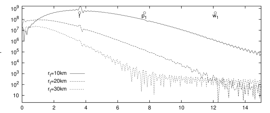
Figure 5.18: Fourier transformation of the wave forms for $v_{0}=0.5$.

Figure 5.19: Fourier transformation of the wave form for $r_{t}=10$km and $v_{0}=0.97$. The scales are arbitrary. The presence of the first $w$-mode is clearly visible.

5.5 Discussion

With the particle we have a physical even though probably a quite unrealistic process, which induces oscillations in a neutron star. By unrealistic we mean that this mechanism is unlikely to generate gravitational waves that are strong enough to be detectable on Earth.

Whereas all the considered kinds of initial data of Chapter 4 could excite the $f$-mode and some of the first $p$-modes, this was not the case for the $w$-modes. There, only a special class of initial data was able to excite those modes.

Andersson and Kokkotas [55] have shown how to extract the physical parameters of a neutron star, like mass $M$ and radius $R$ and possibly the equation of state, if the complex frequencies of the $f$-mode and the first $w$-mode are known. Of course, it is only possible to detect the first $w$-mode of a neutron star if it gets excited by some physical mechanism.

We used an orbiting mass $\mu$ in the particle limit $\mu\ll M$ to assess whether or not it is possible to excite the first $w$-mode. We found that in order to excite a significant amount of $w$-modes the particle’s velocity at infinity must be much more than 70 percent of the speed of light. Moreover, the excitation strength of the modes rapidly decreases as the particle’s turning point $r_{t}$ increases. This is in agreement with the results of Ferrari et al. [65], who find that no significant $w$-mode excitation is observable. However, they do not consider the cases where the particle has an energy $E\gg 1$, which is necessary if it were to excite any $w$-modes.

The question now arises: Can we infer anything about what happens in an astrophysical event? Our results show that the particle initially has to be incredibly fast in order to excite a significant amount of $w$-mode content. It is clear that there do not exist any astrophysical events at all that could accelerate the particle (which, of course does not represent an elementary particle, but some heavy extended object, like a planet or an asteroid or even another neutron star) up to more than half the speed of light. Hence, we might safely conclude that any astrophysical scenario that can be simulated by a particle orbiting a neutron star will not produce any detectable amount of $w$-modes.

But what if the object collides with the neutron star? It has been suggested [65] that in this case there might be some significant excitation of $w$-modes. In particular, simulations of a particle that radially falls onto a neutron star were done by Borelli [64] who found that, indeed, both fluid and $w$-modes were excited to a significant level. However, one serious drawback of those calculations is that as soon as the particle hits the surface of the star, the calculation is stopped. This leads to an overestimation of the high frequency components in the power spectrum. Besides, in this study only axial modes were investigated, it is therefore clear that the $w$-modes will always show up in the spectrum because they will not be screened by the presence of fluid modes, which can happen in the even parity case. Now, even in the particle limit, it is not possible to simulate a collision since it not clear at all what happens when the particle hits the surface. A first step might be, though, to let the particle go right through the neutron star without being affected by the presence of the neutron star matter. In case there is a significant amount of $w$-modes one might conclude that in a realistic scenario, where the physics of the impact is included, there still might be $w$-modes present, maybe they are even more strongly excited than in the unphysical “tunnelling” case. However, our view is that even in the impact case the particle still must have an initial velocity that is a significant fraction of the speed of light. Since for scattering orbits with initial speeds less than 50 percent of the speed of light there is no hint of any $w$-mode presence even for the closest trajectories, we believe that this should not change very much even if the particle’s turning point lies inside the neutron star. Of course, in this case it seems reasonable to infer that the $p$-modes of the fluid would be much more strongly excited.

Our results in chapter 4 indicate that the presence of the $w$-modes in the signal is closely related with the value of $S$. This particular role of $S$ seems also to be confirmed in our particle simulations, for we have seen that for ultra-relativistic particles the value of $rS$ greatly dominates the value of $T/r$. And it is only there that we find a significant amount of $w$-modes.

Still, the question remains as to what happens in a realistic astrophysical scenario. We have excluded the possibility of $w$-modes excitation by means of a realistic scattering process. However, it is not possible to confer our results to the merger process of a binary neutron star system, for the latter cannot be adequately described within perturbation theory. Only if the final object does not immediately collapse to a black hole, it might wildly oscillate and emit some significant radiation through $w$-modes.

Appendix A Relations between the Regge-Wheeler and Mathews-Zerilli harmonics

The evolution equations (5.6) will be expanded using the Regge-Wheeler harmonics $[{\cal\char 89\relax}^{A}_{lm}]_{\mu\nu}$, which are defined in [17], and which do not form an orthonormal set. However, in order to perform the expansion of the energy-momentum tensor (5.1), we need an orthonormal set. This is given by the Mathews-Zerilli harmonics $[\widehat{\cal\char 89\relax}^{A}_{lm}]_{\mu\nu}$ [74, 23], which are orthonormal with respect to the following inner product

$$\int_{S^{2}}[\widehat{\cal\char 89\relax}^{A}_{lm}]^{*\mu\nu}[\widehat{\cal\char 89\relax}^{A^{\prime}}_{l^{\prime}m^{\prime}}]_{\mu\nu}\,{\rm d\Omega}\; =\;s_{A}\delta_{AA^{\prime}}\delta_{ll^{\prime}}\delta_{mm^{\prime}}\;,$$ (A.1)

where the asterisk denotes complex conjugation and

$$[\widehat{\cal\char 89\relax}^{A}_{lm}]^{\mu\nu}\; =\;\eta^{\mu\kappa}\eta^{\nu\sigma}[\widehat{\cal\char 89\relax}^{A}_{lm}]_{\kappa\sigma}\;.$$ (A.2)

Because of the use of the inverse Minkowski metric $\eta^{\mu\nu}$ to raise the indices, the inner product (A.1) is not positive definite and it is

$$s_{A}\; =\;\begin{cases}+1,&A=1,5,\dots,10\\ -1,&A=2,3,4\\ \end{cases}\;.$$ (A.3)

For the sake of completeness we list the whole set of the 10 tensor harmonics $\widehat{\cal\char 89\relax}^{A}_{lm}$, where we correct some errors in [61]:

$$[\widehat{\cal\char 89\relax}^{1}_{lm}]_{\mu\nu}\; =\;\left(\begin{array}[]{cccc}1&0&0&0\\ 0&0&0&0\\ 0&0&0&0\\ 0&0&0&0\\ \end{array}\right)Y_{lm}$$

$${}[\widehat{\cal\char 89\relax}^{2}_{lm}]_{\mu\nu}\; =\;\frac{\mbox{i}}{\sqrt{2}}\left(\begin{array}[]{cccc}0&1&0&0\\ 1&0&0&0\\ 0&0&0&0\\ 0&0&0&0\\ \end{array}\right)Y_{lm}$$

$${}[\widehat{\cal\char 89\relax}^{3}_{lm}]_{\mu\nu}\; =\;\frac{\mbox{i}r}{\sqrt{2l(l+1)}}\left(\begin{array}[]{cccc}0&0&\frac{\partial{}}{\partial{\theta}}&\frac{\partial{}}{\partial{\phi}}\\ 0&0&0&0\\ \frac{\partial{}}{\partial{\theta}}&0&0&0\\ \frac{\partial{}}{\partial{\phi}}&0&0&0\\ \end{array}\right)Y_{lm}$$

$${}[\widehat{\cal\char 89\relax}^{4}_{lm}]_{\mu\nu}\; =\;\frac{r}{\sqrt{2l(l+1)}}\left(\begin{array}[]{cccc}0&0&\frac{1}{\sin\theta}\frac{\partial{}}{\partial{\phi}}&-\sin\theta\frac{\partial{}}{\partial{\theta}}\\ 0&0&0&0\\ \frac{1}{\sin\theta}\frac{\partial{}}{\partial{\phi}}&0&0&0\\ -\sin\theta\frac{\partial{}}{\partial{\theta}}&0&0&0\\ \end{array}\right)Y_{lm}$$

$${}[\widehat{\cal\char 89\relax}^{5}_{lm}]_{\mu\nu}\; =\;\left(\begin{array}[]{cccc}0&0&0&0\\ 0&1&0&0\\ 0&0&0&0\\ 0&0&0&0\\ \end{array}\right)Y_{lm}$$

$${}[\widehat{\cal\char 89\relax}^{6}_{lm}]_{\mu\nu}\; =\;\frac{r}{\sqrt{2l(l+1)}}\left(\begin{array}[]{cccc}0&0&0&0\\ 0&0&\frac{\partial{}}{\partial{\theta}}&\frac{\partial{}}{\partial{\phi}}\\ 0&\frac{\partial{}}{\partial{\theta}}&0&0\\ 0&\frac{\partial{}}{\partial{\phi}}&0&0\\ \end{array}\right)Y_{lm}$$

$${}[\widehat{\cal\char 89\relax}^{7}_{lm}]_{\mu\nu}\; =\;\frac{\mbox{i}r}{\sqrt{2l(l+1)}}\left(\begin{array}[]{cccc}0&0&0&0\\ 0&0&\frac{1}{\sin\theta}\frac{\partial{}}{\partial{\phi}}&-\sin\theta\frac{\partial{}}{\partial{\theta}}\\ 0&\frac{1}{\sin\theta}\frac{\partial{}}{\partial{\phi}}&0&0\\ 0&-\sin\theta\frac{\partial{}}{\partial{\theta}}&0&0\\ \end{array}\right)Y_{lm}$$

$${}[\widehat{\cal\char 89\relax}^{8}_{lm}]_{\mu\nu}\; =\;\frac{r^{2}}{\sqrt{2l(l+1)(l-1)(l+2)}}\left(\begin{array}[]{cccc}0&0&0&0\\ 0&0&0&0\\ 0&0&W_{lm}&X_{lm}\\ 0&0&X_{lm}&-\sin^{2}\theta\,W_{lm}\\ \end{array}\right)\;,$$

$${}[\widehat{\cal\char 89\relax}^{9}_{lm}]_{\mu\nu}\; =\;\frac{r^{2}}{\sqrt{2}}\left(\begin{array}[]{cccc}0&0&0&0\\ 0&0&0&0\\ 0&0&1&0\\ 0&0&0&\sin^{2}\theta\\ \end{array}\right)Y_{lm}$$

$${}[\widehat{\cal\char 89\relax}^{10}_{lm}]_{\mu\nu}\; =\;\frac{\mbox{i}r^{2}}{\sqrt{2l(l+1)(l-1)(l+2)}}\left(\begin{array}[]{cccc}0&0&0&0\\ 0&0&0&0\\ 0&0&\frac{1}{\sin\theta}\,X_{lm}&-\sin\theta\,W_{lm}\\ 0&0&-\sin\theta\,W_{lm}&-\sin\theta\,X_{lm}\\ \end{array}\right)$$

with

$$X_{lm}\; :=\;2\left(\frac{\partial{}}{\partial{\theta}}-\cot\theta\right)\frac{\partial{}}{\partial{\phi}}Y_{lm}$$ (A.4)

$$W_{lm}\; :=\;\left(\frac{\partial^{2}{}}{\partial{\theta}^{2}}-\cot\theta\frac{\partial{}}{\partial{\theta}}-\frac{1}{\sin^{2}\theta}\frac{\partial^{2}{}}{\partial{\phi}^{2}}\right)Y_{lm}\;=\;\left(l(l+1)+2\frac{\partial^{2}{}}{\partial{\theta}^{2}}\right)Y_{lm}\;,$$ (A.5)

and $Y_{lm}$ are the ordinary scalar harmonics. There are three odd parity harmonics $\widehat{\cal\char 89\relax}^{4}_{lm},\widehat{\cal\char 89\relax}^{7}_{lm}$ and $\widehat{\cal\char 89\relax}^{10}_{lm}$, the remaining seven ones have even parity.

In terms of the Mathews-Zerilli harmonics $\widehat{\cal\char 89\relax}^{A}_{lm}$ the Regge-Wheeler harmonics ${\cal\char 89\relax}^{A}_{lm}$ read:

$${\cal\char 89\relax}^{1}_{lm}\; =\;\widehat{\cal\char 89\relax}^{1}_{lm}$$

$${\cal\char 89\relax}^{2}_{lm}\; =\;-\mbox{i}\sqrt{2}\,\widehat{\cal\char 89\relax}^{2}_{lm}$$

$${\cal\char 89\relax}^{3}_{lm}\; =\;-\frac{\mbox{i}}{r}\sqrt{2l(l+1)}\,\widehat{\cal\char 89\relax}^{3}_{lm}$$

$${\cal\char 89\relax}^{4}_{lm}\; =\;-\frac{1}{r}\sqrt{2l(l+1)}\,\widehat{\cal\char 89\relax}^{4}_{lm}$$

$${\cal\char 89\relax}^{5}_{lm}\; =\;\widehat{\cal\char 89\relax}^{5}_{lm}$$

$${\cal\char 89\relax}^{6}_{lm}\; =\;\frac{1}{r}\sqrt{2l(l+1)\,}\widehat{\cal\char 89\relax}^{6}_{lm}$$

$${\cal\char 89\relax}^{7}_{lm}\; =\;\frac{\mbox{i}}{r}\sqrt{2l(l+1)}\,\widehat{\cal\char 89\relax}^{7}_{lm}$$

$${\cal\char 89\relax}^{8}_{lm}\; =\;\frac{\sqrt{2}}{2r^{2}}l(l+1)\left(\sqrt{\frac{(l-1)(l+2)}{l(l+1)}}\,\widehat{\cal\char 89\relax}^{8}_{lm}-\widehat{\cal\char 89\relax}^{9}_{lm}\right)$$

$${\cal\char 89\relax}^{9}_{lm}\; =\;\frac{\sqrt{2}}{r^{2}}\,\widehat{\cal\char 89\relax}^{9}_{lm}$$

$${\cal\char 89\relax}^{10}_{lm}\; =\;\frac{i}{2r^{2}}\sqrt{2l(l+1)(l-1)(l+2)}\,\widehat{\cal\char 89\relax}^{10}_{lm}\;.$$

The inverse relations are given by

$${}\widehat{\cal\char 89\relax}^{1}_{lm}\; =\;{\cal\char 89\relax}^{1}_{lm}$$

$${}\widehat{\cal\char 89\relax}^{2}_{lm}\; =\;\frac{\mbox{i}}{\sqrt{2}}\,{\cal\char 89\relax}^{2}_{lm}$$

$${}\widehat{\cal\char 89\relax}^{3}_{lm}\; =\;\frac{\mbox{i}r}{\sqrt{2l(l+1)}}\,{\cal\char 89\relax}^{3}_{lm}$$

$${}\widehat{\cal\char 89\relax}^{4}_{lm}\; =\;-\frac{r}{\sqrt{2l(l+1)}}\,{\cal\char 89\relax}^{4}_{lm}$$

$${}\widehat{\cal\char 89\relax}^{5}_{lm}\; =\;{\cal\char 89\relax}^{5}_{lm}$$

$${}\widehat{\cal\char 89\relax}^{6}_{lm}\; =\;\frac{r}{\sqrt{2l(l+1)}}\,{\cal\char 89\relax}^{6}_{lm}$$

$${}\widehat{\cal\char 89\relax}^{7}_{lm}\; =\;-\frac{\mbox{i}r}{\sqrt{2l(l+1)}}\,{\cal\char 89\relax}^{7}_{lm}$$

$${}\widehat{\cal\char 89\relax}^{8}_{lm}\; =\;\frac{r^{2}}{\sqrt{2l(l+1)(l-1)(l+2)}}\left(l(l+1)\,{\cal\char 89\relax}^{9}_{lm}+2\,{\cal\char 89\relax}^{8}_{lm}\right)$$

$${}\widehat{\cal\char 89\relax}^{9}_{lm}\; =\;\frac{r^{2}}{\sqrt{2}}\,{\cal\char 89\relax}^{9}_{lm}$$

$${}\widehat{\cal\char 89\relax}^{10}_{lm}\; =\;-\frac{2\mbox{i}r^{2}}{\sqrt{2l(l+1)(l-1)(l+2)}}\,{\cal\char 89\relax}^{10}_{lm}\;.$$

Appendix B The source terms of the particle

The particle’s energy-momentum tensor (5.1) will be expanded using the orthonormal Mathews-Zerilli harmonics defined in appendix A:

$${\cal T}_{\mu\nu}\; =\;\sum_{l=0}^{\infty}\sum_{m=-l}^{l}\sum_{A=1}^{10}\hat{t}^{lm}_{A}[\widehat{\cal\char 89\relax}^{A}_{lm}]_{\mu\nu}\;.$$ (B.1)

By using the orthonormality condition (A.1) we can compute the coefficients $\hat{t}^{lm}_{A}$ through

$$\hat{t}_{A}^{lm}\; =\;\int_{S^{2}}[\widehat{\cal\char 89\relax}^{A}_{lm}]^{*\mu\nu}{\cal T}_{\mu\nu}\,{\rm d\Omega}\;.$$ (B.2)

We thus obtain the following set:

$$\hat{t}_{1}^{lm}\; =\;e^{4\nu}\frac{\mu}{r^{2}}\frac{dt}{d\tau}\delta(r-R(t))Y^{*}_{lm}$$

$$\hat{t}_{2}^{lm}\; =\;\mbox{i}\sqrt{2}\frac{\mu}{r^{2}}\frac{dR}{d\tau}\delta(r-R(t))Y^{*}_{lm}$$

$$\hat{t}_{3}^{lm}\; =\;e^{2\nu}\frac{2\mbox{i}\mu}{r\sqrt{2l(l+1)}}\delta(r-R(t))\frac{d}{d\tau}Y^{*}_{lm}$$

$$\hat{t}_{4}^{lm}\; =\;e^{2\nu}\frac{2\mu}{r\sqrt{2l(l+1)}}\delta(r-R(t))\left(\frac{1}{\sin\Theta}\frac{d\Theta}{d\tau}\frac{\partial{}}{\partial{\Phi}}-\sin\Theta\frac{d\Phi}{d\tau}\frac{\partial{}}{\partial{\Theta}}\right)Y^{*}_{lm}$$

$$\hat{t}_{5}^{lm}\; =\;e^{4\lambda}\frac{\mu}{r^{2}}\frac{d\tau}{dt}\left(\frac{dR}{d\tau}\right)^{2}\delta(r-R(t))Y^{*}_{lm}$$

$$\hat{t}_{6}^{lm}\; =\;e^{2\lambda}\frac{2\mu}{r\sqrt{2l(l+1)}}\frac{d\tau}{dt}\frac{dR}{d\tau}\delta(r-R(t))\frac{d}{d\tau}Y^{*}_{lm}$$

$$\hat{t}_{7}^{lm}\; =\;e^{2\lambda}\frac{2\mbox{i}\mu}{r\sqrt{2l(l+1)}}\frac{d\tau}{dt}\frac{dR}{d\tau}\delta(r-R(t))\left(\sin\Theta\frac{d\Phi}{d\tau}\frac{\partial{}}{\partial{\Theta}}-\frac{1}{\sin\Theta}\frac{d\Theta}{d\tau}\frac{\partial{}}{\partial{\Phi}}\right)Y^{*}_{lm}$$

$$\begin{split}\hat{t}_{8}^{lm}\;&=\;\frac{\mu}{\sqrt{2l(l+1)(l-1)(l+2)}}\frac{d\tau}{dt}\delta(r-R(t))\\ &\quad\left[\left(\left(\frac{d\Theta}{d\tau}\right)^{2}-\sin^{2}\Theta\left(\frac{d\Phi}{d\tau}\right)^{2}\right)W^{*}_{lm}+2\frac{d\Theta}{d\tau}\frac{d\Phi}{d\tau}X^{*}_{lm}\right]\end{split}$$

$$\hat{t}_{9}^{lm}\; =\;\frac{\mu}{\sqrt{2}}\frac{d\tau}{dt}\delta(r-R(t))\left(\left(\frac{d\Theta}{d\tau}\right)^{2}+\sin^{2}\Theta\left(\frac{d\Phi}{d\tau}\right)^{2}\right)Y^{*}_{lm}$$

$$\begin{split}\hat{t}_{10}^{lm}\;&=\;\frac{\mbox{i}\mu}{\sqrt{2l(l+1)(l-1)(l+2)}}\frac{d\tau}{dt}\delta(r-R(t))\sin\Theta\\ &\quad\left[\left(\left(\frac{d\Phi}{d\tau}\right)^{2}-\frac{1}{\sin^{2}\Theta}\left(\frac{d\Theta}{d\tau}\right)^{2}\right)X^{*}_{lm}+2\frac{d\Theta}{d\tau}\frac{d\Phi}{d\tau}W^{*}_{lm}\right]\;.\end{split}$$

Here, $Y^{*}_{lm},W^{*}_{lm}$ and $X^{*}_{lm}$ are functions of the particle’s angular position $\Theta$ and $\Phi$ parametized by the coordinate time $t$, therefore all derivatives with respect to proper time $\tau$ are to be understood as

$$\frac{d}{d\tau}=\frac{dt}{d\tau}\frac{d}{dt}\;.$$ (B.3)

Since for the decomposition of the evolution equations we use the Regge-Wheeler harmonics ${\cal\char 89\relax}^{A}_{lm}$, which do not form an orthonormal set, we have to expand the energy-momentum tensor (5.1) in Regge-Wheeler harmonics as well:

$${\cal T}_{\mu\nu}\; =\;\sum_{l=0}^{\infty}\sum_{m=-l}^{l}\sum_{A=1}^{10}t^{lm}_{A}[{\cal\char 89\relax}^{A}_{lm}]_{\mu\nu}\;.$$ (B.4)

Of course, we cannot obtain the Regge-Wheeler coefficients $t^{lm}_{A}$ by means of a formula similar to (B.2), but we can construct them from the Mathews-Zerilli coefficients $\hat{t}_{A}^{lm}$. Using the relationship between the different sets of tensor harmonics given in Appendix A, we find:

$$t_{1}^{lm}\; =\;\hat{t}_{1}^{lm}$$

$$t_{2}^{lm}\; =\;\frac{\mbox{i}}{\sqrt{2}}\hat{t}_{2}^{lm}$$

$$t_{3}^{lm}\; =\;\frac{\mbox{i}r}{\sqrt{2l(l+1)}}\hat{t}_{3}^{lm}$$

$$t_{4}^{lm}\; =\;-\frac{r}{\sqrt{2l(l+1)}}\hat{t}_{4}^{lm}$$

$$t_{5}^{lm}\; =\;\hat{t}_{5}^{lm}$$

$$t_{6}^{lm}\; =\;\frac{r}{\sqrt{2l(l+1)}}\hat{t}_{6}^{lm}$$

$$t_{7}^{lm}\; =\;-\frac{\mbox{i}r}{\sqrt{2l(l+1)}}\hat{t}_{7}^{lm}$$

$$t_{8}^{lm}\; =\;\frac{2r^{2}}{\sqrt{2l(l+1)(l-1)(l+2)}}\hat{t}_{8}^{lm}$$

$$t_{9}^{lm}\; =\;\frac{r^{2}}{\sqrt{2}}\left(\hat{t}_{9}^{lm}+\sqrt{\frac{l(l+1)}{(l-1)(l+2)}}\hat{t}_{8}^{lm}\right)$$

$$t_{10}^{lm}\; =\;-\frac{2\mbox{i}r^{2}}{\sqrt{2l(l+1)(l-1)(l+2)}}\hat{t}_{10}^{lm}\;.$$

We now restrict the motion of the particle to the equatorial plane $\Theta=\frac{\pi}{2}$. In this case it is $\frac{d\Theta}{d\tau}=0$ and $\sin\Theta=1$, and we can use the geodesic equations (5.3a) and (5.3c) to substitute all expressions containing derivatives with respect to proper time $\tau$. Furthermore, we can obtain quite simple relations for the derivatives of $Y^{*}_{lm}$:

$$\frac{\partial{}}{\partial{\Phi}}Y^{*}_{lm}\; =\;-\mbox{i}mY^{*}_{lm}$$ (B.5)

$$\frac{\partial^{2}{}}{\partial{\Theta}^{2}}Y^{*}_{lm}\; =\;\left(m^{2}-l(l+1)\right)Y^{*}_{lm}\;.$$ (B.6)

This then gives us a somewhat simpler set of coefficients:

$$t_{1}^{lm}\; =\;e^{2\nu}\frac{\mu E}{r^{2}}\delta(r-R(t))Y^{*}_{lm}$$

$$t_{2}^{lm}\; =\;-e^{2\lambda}\frac{\mu E}{r^{2}}v(t)\delta(r-R(t))Y^{*}_{lm}$$

$$t_{3}^{lm}\; =\;e^{2\nu}\frac{\mbox{i}m\mu L}{r^{2}l(l+1)}\delta(r-R(t))Y^{*}_{lm}$$

$$t_{4}^{lm}\; =\;e^{2\nu}\frac{\mu L}{r^{2}l(l+1)}\delta(r-R(t))\frac{\partial{}}{\partial{\Theta}}Y^{*}_{lm}$$

$$t_{5}^{lm}\; =\;e^{6\lambda}\frac{\mu E}{r^{2}}v^{2}(t)\delta(r-R(t))Y^{*}_{lm}$$

$$t_{6}^{lm}\; =\;-e^{2\lambda}\frac{\mbox{i}m\mu L}{r^{2}l(l+1)}v(t)\delta(r-R(t))Y^{*}_{lm}$$

$$t_{7}^{lm}\; =\;e^{2\lambda}\frac{\mu L}{r^{2}l(l+1)}v(t)\delta(r-R(t))\frac{\partial{}}{\partial{\Theta}}Y^{*}_{lm}$$

$$t_{8}^{lm}\; =\;e^{2\nu}\frac{\mu L^{2}(l(l+1)-2m^{2})}{r^{2}El(l+1)(l-1)(l+2)}\delta(r-R(t))Y^{*}_{lm}$$

$$t_{9}^{lm}\; =\;e^{2\nu}\frac{\mu L^{2}(l(l+1)-m^{2}-1)}{r^{2}E(l-1)(l+2)}\delta(r-R(t))Y^{*}_{lm}$$

$$t_{10}^{lm}\; =\;-e^{2\nu}\frac{2\mbox{i}m\mu L^{2}}{r^{2}El(l+1)(l-1)(l+2)}\delta(r-R(t))\frac{\partial{}}{\partial{\Theta}}Y^{*}_{lm}\;,$$

where $v(t)=\frac{dR}{dt}$ is the radial velocity of the particle. The field equations also require the computation of the trace

$${\cal T}\; =\;g^{\mu\nu}{\cal T}_{\mu\nu}\;=\;\sum_{l,m}t^{lm}Y_{lm}\;,$$ (B.7)

with

$$t^{lm}\; =\;-e^{2\lambda}t_{1}^{lm}+e^{-2\lambda}t_{5}^{lm}-\frac{l(l+1)}{r^{2}}t_{8}^{lm}+\frac{2}{r^{2}}t_{9}^{lm}\;.$$ (B.8)

Using the explicit forms of the coefficients, we obtain

$$t^{lm}\; =\;\frac{\mu}{r^{2}}\delta(r-R(t))\left(Ev^{2}(t)e^{4\lambda}-E+e^{2\nu}\frac{L^{2}}{r^{2}E}\right)Y^{*}_{lm}\;,$$ (B.9)

and by making use of the geodesic equation (5.3b) we can reduce this expression to

$$t^{lm}\; =\;-e^{2\nu}\frac{\mu}{r^{2}E}\delta(r-R(t))Y^{*}_{lm}\;.$$ (B.10)

Appendix C Derivation of the radiation extraction formula

The radiated energy emitted per unit time and unit angle is given by [3]

$$\frac{d^{2}E}{dt\,d\Omega} =\frac{r^{2}}{16\pi}\left[\left(\frac{\partial{}}{\partial{t}}h_{[\theta][\phi]}\right)^{2}+\frac{1}{4}\left(\frac{\partial{}}{\partial{t}}h_{[\theta][\theta]}-\frac{\partial{}}{\partial{t}}h_{[\phi][\phi]}\right)^{2}\right]\;,$$ (C.1)

where

$$h_{[i][j]}\; :=\;\sqrt{g^{ii}g^{jj}}\,h_{ij}\;,$$ (C.2)

or specifically

$$h_{[\theta][\phi]} =\frac{1}{r^{2}\sin\theta}h_{\theta\phi}$$ (C.3)

$$h_{[\theta][\theta]} =\frac{1}{r^{2}}h_{\theta\theta}$$ (C.4)

$$h_{[\phi][\phi]} =\frac{1}{r^{2}\sin^{2}\theta}h_{\phi\phi}\;.$$ (C.5)

The metric components $h_{[i][j]}$ have to be in the radiation gauge, which asserts that only

$$h_{[\theta][\phi]} ={\cal O}(1/r)$$ (C.6)

$$h_{[\theta][\theta]}-h_{[\phi][\phi]} ={\cal O}(1/r)\;,$$ (C.7)

whereas all other components must fall off faster than ${\cal O}(1/r)$. Furthermore, it must hold that $h_{[\theta][\theta]}=-h_{[\phi][\phi]}+{\cal O}(1/r^{2})$. We now expand the angular parts of the metric into the orthonormal Mathews-Zerilli tensor harmonics given in Appendix A. Since we focus on the polar perturbations, we only need to consider $\widehat{\cal\char 89\relax}_{8}^{lm}$ and $\widehat{\cal\char 89\relax}_{9}^{lm}$, and we have

$$h_{[i][j]} =\sum_{l,m}\left(\begin{array}[]{cc}\left(\frac{1}{\sqrt{2}}{\widehat{K}}_{lm}Y_{lm}+\frac{1}{N}{\widehat{G}}_{lm}W_{lm}\right)&\frac{1}{N\sin\theta}{\widehat{G}}_{lm}X_{lm}\\ \frac{1}{N\sin\theta}{\widehat{G}}_{lm}X_{lm}&\left(\frac{1}{\sqrt{2}}{\widehat{K}}_{lm}Y_{lm}-\frac{1}{N}{\widehat{G}}_{lm}W_{lm}\right)\\ \end{array}\right)\;,$$ (C.10)

where we use

$$N:=\sqrt{2l(l+1)(l-1)(l+2)}\;.$$ (C.11)

This gives us

$$\frac{d^{2}E}{dtd\Omega} =\frac{r^{2}}{16\pi}\left(\left\lvert\sum_{l,m}\frac{\dot{\widehat{G}}_{lm}}{N^{2}\sin^{2}\theta}X_{lm}\right\rvert^{2}+\left\lvert\sum_{l,m}\frac{\dot{\widehat{G}}_{lm}}{N^{2}}W_{lm}\right\rvert^{2}\right)\;,$$ (C.12)

where we have to take the square moduli because we are dealing with complex metric coefficients. To obtain the total energy flux, we have to integrate over a 2-sphere

$$\frac{dE}{dt} =\frac{r^{2}}{16\pi}\sum_{l,m,l^{\prime},m^{\prime}}\frac{1}{N^{2}}\dot{\widehat{G}}_{lm}\dot{\widehat{G}}_{*l^{\prime}m^{\prime}}\int_{S^{2}}\left(\frac{X_{lm}X^{*}_{l^{\prime}m^{\prime}}}{\sin^{2}\theta}+W_{lm}W^{*}_{l^{\prime}m^{\prime}}\right)d\Omega\;.$$ (C.13)

Now, because of the orthonormality relation the integral is just

$$\int_{S^{2}}\left(\frac{X_{lm}X^{*}_{l^{\prime}m^{\prime}}}{\sin^{2}\theta}+W_{lm}W^{*}_{l^{\prime}m^{\prime}}\right)d\Omega =\frac{1}{2}N^{2}\delta_{ll^{\prime}}\delta_{mm^{\prime}}\;,$$ (C.14)

and we obtain

$$\frac{dE}{dt} =\frac{r^{2}}{32\pi}\sum_{l,m}|\dot{\widehat{G}}_{lm}|^{2}\;.$$ (C.15)

Since the actual metric perturbations are derived using the expansion into the Regge-Wheeler harmonics, we have to express (C.15) in terms of those variables. The relation between $\widehat{G}_{lm}$ and the Regge-Wheeler variable $G_{lm}$ is easily derived to be

$$\widehat{G}_{lm} =\frac{N}{2}G_{lm}\;,$$ (C.16)

which leads to the following radiation formula

$$\frac{dE}{dt} =\frac{r^{2}}{64\pi}\sum_{l,m}l(l+1)(l-1)(l+2)|\dot{G}_{lm}|^{2}\;.$$ (C.17)

Note, however, that $G_{lm}$ is still in the radiation gauge and not in the Regge-Wheeler gauge. In the Regge-Wheeler gauge we have $G_{lm}=0$, and the above formula would not make any sense. We now have to devise a way which relates $G_{lm}$ to the variables in the Regge-Wheeler gauge. This can be accomplished as follows. Following Moncrief [28], we construct some gauge invariant quantities, in particular the Zerilli function, and examine their asymptotic behavior. We then will show that the Zerilli function has the same asymptotic behavior as $G_{lm}$ in the radiation gauge. Hence, the radiated power is proportional to the time derivative of the Zerilli function, which can be easily constructed from the metric variables in the Regge-Wheeler gauge.

Let us write the general expansion of the even parity perturbations of the spacial part of the metric in terms of Regge-Wheeler harmonics (Here we use the notation of Moncrief and focus on fixed values $l$ and $m$:)

$$h_{rr} =e^{2\lambda}H_{2}Y_{lm}$$ (C.18)

$$h_{r\theta} =h_{1}\frac{\partial{Y_{lm}}}{\partial{\theta}},\quad h_{r\phi}\;=\;h_{1}\frac{\partial{Y_{lm}}}{\partial{\phi}}$$ (C.19)

$$h_{\theta\theta} =r^{2}\left(KY_{lm}+G\frac{\partial^{2}{Y_{lm}}}{\partial{\theta}^{2}}\right)$$ (C.20)

$$h_{\theta\phi} =\frac{r^{2}}{2}GX_{lm}$$ (C.21)

$$h_{\phi\phi} =r^{2}\sin^{2}\theta\left(KY_{lm}-G\left(l(l+1)Y_{lm}+\frac{\partial^{2}{Y_{lm}}}{\partial{\theta}^{2}}\right)\right)\;.$$ (C.22)

We can then construct the following gauge invariant quantity

$$q_{1}:=4re^{-4\lambda}k_{2}+rl(l+1)k_{1}\;,$$ (C.23)

where

$$k_{1} =K+e^{-2\lambda}\left(rG^{\prime}-\frac{2}{r}h_{1}\right)$$ (C.24)

and

$$k_{2} =\frac{1}{2}\left(e^{2\lambda}H_{2}-e^{\lambda}\left(re^{\lambda}K\right)^{\prime}\right)\;.$$ (C.25)

We now have to determine the asymptotic behavior of $q_{1}$. To do so, we have to know the asymptotic behavior of the metric coefficients $h_{1}$, $H_{2}$, $K$ and $G$, which, of course, will depend on the chosen gauge. However, because of its gauge invariance, $q_{1}$ will always have the same asymptotic behavior, regardless in what gauge the metric variables are.

Therefore we assume our metric variables to be in the radiation gauge, where we know the asymptotic behavior. Since $h_{[\theta][\theta]}=-h_{[\phi][\phi]}+{\cal O}(1/r^{2})$, the sum $h_{[\theta][\theta]}+h_{[\phi][\phi]}$ has to be of order ${\cal O}(1/r^{2})$, i.e.

$$h_{[\theta][\theta]}+h_{[\phi][\phi]} =\left(2K-l(l+1)G\right)Y_{lm}\;=\;{\cal O}(1/r^{2})\;.$$ (C.26)

But this can only hold if

$$2K =l(l+1)G+{\cal O}(1/r^{2})$$ (C.27)

for the leading order. Using this relation we find for $k_{1}$ and $k_{2}$

$$k_{1}\; \sim\;K+rG^{\prime}\;\sim\;\frac{1}{2}l(l+1)G+rG^{\prime}$$ (C.28)

$$k_{2}\; \sim\;-\frac{1}{2}K-\frac{r}{2}K^{\prime}\;\sim\;-\frac{1}{4}l(l+1)\left(G+rG^{\prime}\right)\;,$$ (C.29)

where “a $\sim$ b” means $a$ equals $b$ plus higher order terms. This leaves us with

$$q_{1}\; \sim\;\frac{r}{2}l(l+1)\left(l(l+1)-2\right)G\;.$$ (C.30)

Moncrief finally defines the quantity

$$Q\; :=\;\frac{q_{1}}{l(l+1)-2+\frac{2M}{r}}\;,$$ (C.31)

which satisfies the Zerilli equation. The leading order for $Q$ is then

$$Q\; \sim\;\frac{r}{2}l(l+1)G\;,$$ (C.32)

which is equivalent to

$$G\; \sim\;\frac{2}{rl(l+1)}Q\;.$$ (C.33)

This relation only holds if $G$ is given in the radiation gauge. But in the radiation formula (C.17) this is the case and we may substitute $G$ by means of (C.33), which yields

$$\frac{dE}{dt} =\frac{1}{16\pi}\sum_{l,m}\frac{(l-1)(l+2)}{l(l+1)}|\dot{Q}_{lm}|^{2}\;.$$ (C.34)

We now have to express $Q$ in terms of our actual perturbation variables $S$ and $T$, which are in the Regge-Wheeler gauge. We first recall that in the Regge-Wheeler gauge, it is

$$h_{1} =0$$ (C.35)

$$H_{2} =\frac{T}{r}+rS$$ (C.36)

$$K =\frac{T}{r}$$ (C.37)

$$G =0\;.$$ (C.38)

Then we compute $k_{1}$ and $k_{2}$, which is readily done:

$$k_{1} =\frac{T}{r}$$ (C.39)

$$k_{2} =\frac{1}{2}\left(e^{2\lambda}\left(\frac{T}{r}+rS\right)-e^{\lambda}\left(e^{\lambda}T\right)^{\prime}\right)\;.$$ (C.40)

Next is $q_{1}$

$$q_{1} =2re^{-4\lambda}\left(e^{2\lambda}\left(\frac{T}{r}+rS\right)-e^{\lambda}\left(e^{\lambda}T\right)^{\prime}\right)+l(l+1)T$$ (C.41)

$$=2e^{-2\lambda}\left(\left(1-r\lambda^{\prime}\right)T+r^{2}S-T^{\prime}\right)+l(l+1)T\;.$$ (C.42)

Using

$$\lambda^{\prime}=\frac{M}{r\left(2M-r\right)}$$ (C.43)

and collecting terms yields

$$q_{1} =-\left(1-\frac{2M}{r}\right)\left(2rT^{\prime}+\frac{2M-r\left(2+l(l+1)\right)}{r-2M}T-2r^{2}S\right)\;.$$ (C.44)

If we furthermore define $Z$ to be

$$Z =\frac{2}{l(l+1)}Q\;=\;\frac{2}{l(l+1)}\frac{q_{1}}{l(l+1)-2+\frac{2M}{r}}\;,$$ (C.45)

we find from (C.33) that

$$G\; \sim\;\frac{Z}{r}\;,$$ (C.46)

and the radiation formula (C.34) finally reads

$$\frac{dE}{dt} =\frac{1}{64\pi}\sum_{l,m}l(l+1)(l-1)(l+2)|\dot{Z}_{lm}|^{2}=\frac{1}{64\pi}\sum_{l,m}\frac{(l+2)!}{(l-2)!}|\dot{Z}_{lm}|^{2}\;,$$ (C.47)

with

$$\!\!\!\!\!Z =-\frac{2}{l(l+1)}\frac{1-\frac{2M}{r}}{l(l+1)-2+\frac{6M}{r}}\left(2rT^{\prime}+\frac{2M-r\left(2+l(l+1)\right)}{r-2M}T-2r^{2}S\right)\;,$$ (C.48)

which agrees with our definition of the Zerilli function in (4.38).

Danksagung

Ich danke allen Institutsmitgliedern, voran unseren Systemies, die bereit waren, sich für meine Computer- und Druckerprobleme Zeit zu nehmen und mir dabei weiterzuhelfen.

Ganz herzlich möchte ich mich bei Prof. Dr. Ruder bedanken, der es mir nicht nur durch eine Stelle beim SFB 382 ermöglicht hat, diese Doktorarbeit anzufertigen, sondern auch nie einen Dienstreisewunsch abgeschlagen hat, und sei es bis nach Indien gewesen. Auch danke ich Priv. Doz. Dr. Harald Riffert, der ein hilfsbereiter Ansprechpartner war und stets ein Ohr für Probleme meinerseits hatte. Des weiteren sei Dr. Hans-Peter Nollert erwähnt, der geduldig die verschiedenen Versionen dieser Arbeit Korrektur gelesen und mit seinen Tipps und Kommentaren sehr zu ihrer Vollendung beigetragen hat.

Leider kann ich mich nicht mehr persönlich bei meinem anfänglichen Betreuer Prof. Dr. Heinz Herold bedanken, zu dem ich, bevor er seiner langen Krankheit erlag, jederzeit mit meinen Anliegen kommen konnte, und der mir in vielen Dingen weitergeholfen hat. Heinz, Du fehlst!

Besonderer Dank gilt dem DAAD, da er mir durch ein HSPIII-Stipendium einen Forschungsaufenthalt in den USA an der Penn State University ermöglicht hat.

I thank Pablo Laguna for being my adviser at Penn State University, and for always being open for my questions even at the morning hours, where nobody was supposed to disturb him.

Without having had Michael Sipior as a reliable drinking buddy I would have saved lots of money and would have had much more evenings to do some useless work. Prost Mike!

I also wish to thank Kostas Kokkotas who transformed my suggstion for a short business trip to Greece into a two year Postdoc fellowship, which will give me the possibility to delve into the investigation of oscillations of rotating neutron stars. $\mathnormal{Ev\chi\alpha\rho\iota\sigma\tau\acute{\omega}\;\pi o\lambda\acute{v}}.$ I am looking forward to this new collaboration.

Mein herzlichster Dank geht an meine allerliebste Freundin Sibylla, die die Hochs und Tiefs der letzten Jahre, die nicht nur mit dieser Doktorarbeit verbunden waren, geduldig ertragen hat, und die in guten wie in schlechten Zeiten stets zu mir gehalten hat.

Ein weiteres Dankeschön geht an den Ex-Tatler Uwe Fischer, der meine CD-Sammlung um einige gute Aufnahmen bereichert hat.

Zu guterletzt möchte ich mich bei meinen Eltern bedanken, die mir ein recht sorgenfreies Physikstudium samt einjährigem USA-Aufenthalt in Oregon ermöglicht haben. Besonders danke ich meinem Vater, der sicherlich nicht geglaubt hat, daßer in seinem wohlverdienten Ruhestand nochmals eine Englischarbeit zu korrigieren hätte.

Bibliography

- Monographs and Textbooks
- [1] Y.B. Zel’dovich and I.D. Novikov: Relativistic Astrophysics: Vol. I Stars and Relativity, Chicago Press, 1971.
- [2] C.W. Misner, K.S. Thorne, and J.A. Wheeler: Gravitation, San Francisco: Freeman & Co., 1973.
- [3] L.D. Landau and E.M. Lifshitz: The Classical theory of fields, 4th ed., London: Pergamon Press, 1975.
- [4] S.L. Shapiro and S.A. Teukolsky: Black Holes, White Dwarfs, and Neutron Stars, New York: J. Wiley & Sons,1983.
- [5] H. Riffert, H. Müther, H. Herold, and H. Ruder: Matter at High Densities in Astrophysics, Springer Tracts in Modern Physics, Vol. 133, 1996.
- [6] N.K. Glendenning: Compact Stars, Astronomy and Astrophysics Library, Springer-Verlag, New York, 1997.
- [7] S. Chandrasekhar: The Mathematical Theory of Black Holes, Oxford: Claredon Press, Oxford Classic Texts in the Physical Sciences, 1998.
- [8] W.H. Press, S.A. Teukolsky, W.T. Vetterling, and B.P. Flannery: Numerical Recipes in C, 2nd ed., Cambridge University Press, 1999. Radial Oscillations of Neutron Stars
- [9] S. Chandrasekhar: Dynamical instability of gaseous masses approaching the Schwarzschild limit in general relativity, Phys. Rev. Lett. 12, 114 (1964).
- [10] S. Chandrasekhar: The dynamical instability of gaseous masses approaching the Schwarzschild limit in general relativity, Astrophys. J. 140, 417 (1964).
- [11] J.M. Bardeen, K.S. Thorne, and D.W. Meltzer: A catalogue of methods for studying the normal modes of radial pulsations of general-relativistic stellar models, Astrophys. J. 145, 508 (1966).
- [12] D.W. Meltzer and K.S. Thorne: Normal modes of radial pulsations of stars at the end point of thermonuclear evolution, Astrophys. J. 145, 514 (1966).
- [13] G. Chanmugam: Radial oscillations of zero-temperature white dwarfs and neutron stars below nuclear densities, Astrophys. J. 217, 799 (1977).
- [14] E.N. Glass and L. Lindblom: The radial oscillations of neutron stars, Astrophys. J. 53, 93 (1983) + Erratum, Astrophys. J. Suppl. 71, 173 (1989).
- [15] H.M. Väth and G. Chanmugam: Radial oscillations of neutron stars and strange stars, Astron. Astrophys. 260, 250 (1992).
- [16] D. Gondek, P. Haensel, and J.L. Zdunik: Radial pulsations and stability of protoneutron stars, Astron. Astrophys. 325, 217 (1998). Non-radial Oscillations of Neutron Stars and Black Holes
- [17] T. Regge and J.A. Wheeler: Stability of a Schwarzschild singularity, Phys. Rev. 108, 1063 (1957).
- [18] K.S. Thorne and A. Campolattaro: Non-radial pulsations of general-relativistic stellar models. I. Analytic analysis for , Astrophys. J. 149, 591 (1967) + Erratum, Astrophys. J. 152, 673 (1968).
- [19] K.S. Thorne: Gravitational radiation damping, Phys. Rev. Lett. 21, 320 (1968).
- [20] R. Price and K.S. Thorne: Non-radial pulsations of general-relativistic stellar models. II. Properties of the gravitational waves, Astrophys. J. 155, 163 (1969).
- [21] K.S. Thorne: Non-radial pulsations of general-relativistic stellar models. III. Analytic and numerical results for neutron stars, Astrophys. J. 158, 1 (1969).
- [22] K.S. Thorne: Non-radial pulsations of general-relativistic stellar models. IV. The weak-field limit, Astrophys. J. 158, 997 (1969).
- [23] F.J. Zerilli: Tensor harmonics in canonical form for gravitational radiation and other applications, J. Math. Phys. 11, 2203 (1970).
- [24] F.J. Zerilli: Effective potential for even-parity Regge-Wheeler gravitational perturbation equations, Phys. Rev. Lett. 24, 737 (1970).
- [25] A. Campolattaro and K.S. Thorne: Non-radial pulsations of general-relativistic stellar models. V. Analytic analysis for , Astrophys. J. 159, 847 (1970).
- [26] J.R. Ipser and K.S. Thorne: Non-radial pulsations of general-relativistic stellar models. VI. Corrections, Astrophys. J. 181, 181 (1973).
- [27] S.L. Detweiler and J.R. Ipser: A variational principle and a stability criterion for the neutron star modes of pulsations of stellar models in general relativity, Astrophys. J. 185, 685 (1973).
- [28] V. Moncrief: Gravitational perturbations of spherically symmetric systems. I. The exterior problem, Ann. Phys. 88, 323 (1974).
- [29] V. Moncrief: Gravitational perturbations of spherically symmetric systems. II. Perfect fluid interiors, Ann. Phys. 88, 343 (1974).
- [30] S.L. Detweiler: A variational principle for the fundamental frequencies of quadrupole pulsations of fluid spheres in general relativity, Astrophys. J. 197, 203 (1975).
- [31] S.L. Detweiler: A variational principle and a stability criterion for the dipole modes of pulsations of stellar models in general relativity, Astrophys. J. 201, 440 (1975).
- [32] B.L. Schumaker and K.S. Thorne: Torsional oscillations of neutron stars, Mon. Not. R. Astr. Soc. 203, 457 (1983).
- [33] L. Lindblom and S.L. Detweiler: The quadrupole oscillations of neutron stars, Astrophys. J. Suppl. 53, 73 (1983).
- [34] P.N. McDermott, H.M. Van Horn, and J.F. Scholl: Nonradial -mode oscillations of warm neutron stars, Astrophys. J. 268, 837 (1983).
- [35] P.N. McDermott, C.J. Hansen, H.M. Van Horn, and R. Buland: The non-radial oscillations spectra of neutron stars, Astrophys. J. 297, L37 (1985).
- [36] K.D. Kokkotas and B.F. Schutz: Normal modes of a model radiating system, Gen. Rel. Grav. 18, 913 (1986).
- [37] C. Cutler and L. Lindblom: The effect of viscosity on neutron stars oscillations, Astrophys. J. 314, 234 (1987).
- [38] Y. Kojima: Two families of normal modes in relativistic stars, Prog. Theor. Phys. 79, 665 (1988).
- [39] L. Lindblom and R.J. Splinter: The dipole oscillations of general relativistic neutron stars, Astrophys. J. 345, 925 (1989).
- [40] L.S. Finn: Non-radial pulsations of neutron stars with a crust, Mon. Not. R. Astr. Soc. 245, 82 (1990).
- [41] S. Chandrasekhar and V. Ferrari: On the non-radial oscillations of a star, Proc. R. Soc. London, Ser. A 432, 247 (1991).
- [42] S. Chandrasekhar and V. Ferrari: On the non-radial oscillations of a star. III. A reconsideration of the axial modes, Proc. R. Soc. London, Ser. A 434, 449 (1991).
- [43] J.R. Ipser and R.H. Price: Nonradial pulsations of stellar models in general relativity, Phys. Rev. D 43, 1768 (1991).
- [44] R.H. Price and J.R. Ipser: Relation of gauge formalisms for pulsations of general-relativistic stellar models, Phys. Rev. D 44, 307 (1991).
- [45] K.D. Kokkotas and B.F. Schutz: -modes: A new family of normal modes of pulsating relativistic stars, Mon. Not. R. Astr. Soc. 255, 119 (1992).
- [46] S. Kind and J. Ehlers: Initial-boundary value problem for the spherically symmetric Einstein equations for a perfect fluid, Class. Quantum Grav. 10, 2123 (1993).
- [47] S. Kind, J. Ehlers, and B. Schmidt: Relativistic stellar oscillations treated as an initial value problem, Class. Quantum Grav. 10, 2137 (1993).
- [48] M. Leins, H.-P. Nollert, and M.H. Soffel: Nonradial oscillations of neutron stars: A new branch of strongly damped normal modes, Phys. Rev. D 48, 3467 (1993).
- [49] M. Leins: Nichtradiale Schwingungen von Neutronensternen in der Allgemeinen Relativitätstheorie, Dissertation 1994, Universität Tübingen, unpublished.
- [50] K.D. Kokkotas: Axial modes for relativistic stars, Mon. Not. R. Astr. Soc. 268, 1015 (1994) + Erratum, Mon. Not. R. Astr. Soc. 277, 1599 (1995).
- [51] N. Andersson: Two simple models for gravitational waves modes of compact stars, Gen. Rel. Grav. 28, 1433 (1996).
- [52] N. Andersson, Y. Kojima, and K.D. Kokkotas: On the oscillation spectra of ultracompact stars: An extensive survey of gravitational-wave modes, Astrophys. J. 462, 855 (1996).
- [53] J. Ruoff: Schwingungen von Neutronensternen im Rahmen der (3+1)-Zerlegung, Diplomarbeit 1996, Universität Tübingen, unpublished.
- [54] G. Allen, N. Andersson, K.D. Kokkotas, and B.F. Schutz: Gravitational waves from pulsating stars: Evolving the perturbation equations for a relativistic star, Phys. Rev. D 58, 124012 (1998)
- [55] N. Andersson and K.D. Kokkotas: Towards gravitational wave asteroseismology, Mon. Not. R. Astr. Soc. 299, 1059 (1998).
- [56] N. Andersson: A new class of unstable modes in rotating relativistic stars, Astrophys. J. 502, 708 (1998).
- [57] G. Allen, N. Andersson, K.D. Kokkotas, P. Laguna, J. Pullin, and J. Ruoff: The close-limit approximation to neutron star collisions, Phys. Rev. D 60, 104021 (1999).
- [58] N. Andersson, K.D. Kokkotas, P. Laguna, P. Papadopoulos, and M.S. Sipior: Construction of astrophysical initial data for perturbations of relativistic stars, Phys. Rev. D 60, 124004 (1999).
-
[59]
K.D. Kokkotas and B.G. Schmidt:
Quasi-normal modes of stars and black holes,
[Article in Online Journal Living Reviews in Relativity],
http://www.livingreviews.org/Articles/Volume2/1999-2kokkotas. - [60] H.-P. Nollert: Quasinormal modes: the characteristic ‘sound’ of black holes and neutron stars, Class. Quantum Grav. 16, R159 (1999). Black Holes and Neutron Stars with Orbiting Particles
- [61] F.J. Zerilli: Gravitational field of a particle falling in Schwarzschild geometry analyzed in tensor harmonics, Phys. Rev. D 2, 2141 (1970).
- [62] Y. Kojima: Stellar resonant oscillations coupled to gravitational waves, Prog. Theor. Phys. 77, 297 (1987).
- [63] C. Cutler, L.S. Finn, E. Poisson, and G.J. Sussman: Gravitational radiation from a particle in circular orbit around a black hole. II. Numerical results for the nonrotating case, Phys. Rev. D 47, 1511 (1993).
- [64] A. Borelli: Gravitational radiation emitted when a mass falls onto a compact star, Nuovo Cimento B 112, 225 (1997).
- [65] V. Ferrari, L. Gualtieri, and A. Borelli: Stellar pulsations excited by a scattered mass, Phys. Rev. D 59, 124020 (1999).
- [66] K. Tominaga, M. Saijo, and K. Maeda: Gravitational waves from a test particle scattered by a neutron star: Axial mode case, Phys. Rev. D 60, 024004 (1999).
- [67] Z. Andrade and R.H. Price: Excitation of the odd parity quasi-normal modes of compact objects, Phys. Rev. D 60, 104037 (1999). Rotating neutron stars
- [68] S. Chandrasekhar: Solutions of two problems in the theory of gravitational radiation, Phys. Rev. Lett. 24, 611 (1970).
- [69] S. Chandrasekhar: The effect of gravitational radiation on the secular stability of the Maclaurin spheroid, Astrophys. J. 161, 561 (1970).
- [70] J.L. Friedman and B.F. Schutz: Secular instability of rotating Newtonian stars, Astrophys. J. 222, 281 (1978).
- [71] L. Lindblom: Stellar stability according to Newtonian theory and general relativity, in M. Francaviglia, M. Longhi, L. Lusanna, and E. Sorace, eds., General relativity and gravitation - Proceedings of the GR 14 conference, (1997).
- [72] N. Stergioulas: Rotating stars in relativity, [Article in Online Journal Living Reviews in Relativity], http://www.livingreviews.org/Articles/Volume1/1998-8stergio. Miscellaneous
- [73] R. Arnowitt, S. Deser, and C.W. Misner: The dynamics of general relativity in Gravitation: An Introduction to Current Research, edited by L. Witten (Wiley, New York, 1962), pp. 227–265.
- [74] J. Mathews: Gravitational multipole radiation, J. Soc. Ind. Appl. Math. 10, 768 (1962).
- [75] H.A. Bethe and M. Johnson: Dense baryon matter calculations with realistic potentials, Nucl. Phys. A 230, 1 (1974).
- [76] W.D. Arnett and R.L. Bowers: A microscopic interpretation of neutron star structure, Astrophys. J. Suppl. 33, 415 (1977).
- [77] K.S. Thorne: Multipole expansions of gravitational radiation, Rev. Mod. Phys. 52, 299 (1980).
- [78] B.C. Xanthopoulos: Reducible systems of linear differential equations, Proc. R. Soc. London, Ser. A 378, 61 (1981).
- [79] B.C. Xanthopoulos: Metric and electromagnetic perturbations of the Reissner-Nordström black hole, Proc. R. Soc. London, Ser. A 378, 73 (1981).
- [80] X. Wu, H. Müther, M. Soffel, H.Herold, and H. Ruder: A new equation of state for dense matter and fast rotating pulsars, Astron. Astrophys. 246, 411 (1991).