An efficient filter for detecting gravitational wave bursts in interferometric detectors

Abstract

Typical sources of gravitational wave bursts are supernovae, for which no accurate models exist. This calls for search methods with high efficiency and robustness to be used in the data analysis of foreseen interferometric detectors. A set of such filters is designed to detect gravitational wave burst signals. We first present filters based on the linear fit of whitened data to short straight lines in a given time window and combine them in a non linear filter named ALF. We study the performances and efficiencies of these filters, with the help of a catalogue of simulated supernova signals. The ALF filter is the most performant and most efficient of all filters. Its performance reaches about 80% of the Optimal Filter performance designed for the same signals. Such a filter could be implemented as an online trigger (dedicated to detect bursts of unknown waveform) in interferometric detectors of gravitational waves.

I Introduction

Long baseline interferometric detectors of gravitational waves (GW) [1, 2, 3, 4] will be operational in the next years. The preparation for data analysis with these new instruments has begun since a long time for the compact binary inspirals, the most promising source of GW to date, and for periodic sources as well (see eg [5] for a review). On the other hand, it is important to develop analysis methods to search for GW bursts for which no accurate models exist. Typical sources of GW bursts are supernovae (historically the first cosmic sources of gravitational radiation ever considered). Simulations of collapses of isolated massive stars to neutron stars (type II supernovae) [6, 7, 8, 9] suggest small departures from spherical symmetry. As a consequence, the power radiated away by GW during the few milliseconds of the collapse remains very low : the typical GW amplitude expected for such a source located at 10 Mpc does not exceed $10^{-22}$-$10^{-23}$. This seems to give only hope for detecting supernovae events from inside our Galaxy, given the expected initial sensitivity of the current projects. Collapses of more massive stars to black holes don’t seem to provide much larger amplitudes of GW [10]. One important aspect is that these simulations are unable to predict accurate waveforms for the signals, as a small change in parameters can completely change the shape of the waveform (see [8] for example). This situation calls for search methods with high efficiency and robustness against waveform variations.

Mergers of compact binaries [11] can also be considered as burst sources with perhaps good chances of detection. Some recent estimates for the amplitude of GW during the merging of two neutron stars give numbers as high as a few $10^{-21}$ for sources located at 10 Mpc [12]. The merging of a neutron star and and black hole seems even more efficient with amplitudes near $10^{-20}$ for sources at 10 Mpc [13]. The predicted amplitudes are just above the noise level of initial interferometric detectors, hence a likely detection. Note also that these two kinds of merging compact binaries are likely to be also strong emitters of gamma-ray bursts and, so studies of coincidences between GW detectors and gamma-ray burst detectors on satellites can be crucial to validate the GW detection [14]. Here again, the details of the waveforms in the merging phase are poorly predicted. Finally, concerning the merging of two black holes, the Binary Black Hole Grand Challenge Alliance [15] intends to compute numerically the waveforms emitted during black hole collision and coalescence. Recent results suggest that GW amplitudes could also be of the order of a few $10^{-21}$ for a total binary mass around 10 $M_{\odot}$ located at 10 Mpc [16].

Sources of GW bursts are then characterised by poor predictions of the emitted waveforms. At best, we only have ideas about bandwidths or typical frequencies of the signals. Matched filtering, as used for the detection of inspiralling binaries is clearly ruled out in this case and robust methods for detecting this kind of sources are then required.

Some methods have been recently proposed and studied. The “power filter” technique has been introduced by Flanagan and Hugues [17] in the context of binary black hole mergers, and developed further by Anderson et al. [18, 19]. The idea here is to monitor the noise power along the time; it can be shown that this filter is optimal when only signal duration and bandwidth are known [18, 19]. A similar idea (“Norm Filter”) has been tested independently by Arnaud et al. [20] to detect supernova GW signals. Time-frequency methods [21] should be also pertinent for detecting unmodelled bursts; because of their computing costs, these methods are more suited to the off-line (re-)analysis of candidates selected by faster online algorithms. Of course, one can hardly distinguish between a real burst GW signal and a transient burst caused by noise; thus, methods devoted to detect non stationarity in the noise[22] are then able to detect “true” signals as well. Conversely, general filters are sensitive to transient noises as well as to bursts signals. If selected by on-line triggers, these spurious events can be eliminated if they are coincident with signals detected in auxiliary sensors sensitive to different kinds of environmental noise (seismic activity, RF pickup, …). Otherwise they can be validated when searching for coincidences between candidates from different GW detectors [23]. Furthermore, if an event is seen in coincidence by, say the three interferometers of the LIGO-Virgo network, then it will be possible to reconstruct the characteristics of the emitted GW signal [24]. In particular, the reconstruction of the location of the source in the sky will permit to search for further coincidences with other types of detectors (optical telescopes or gamma-ray satellites for example), and thus enhance the confidence level of the detection.

Our purpose is to develop and test filters for GW burst detection which are efficient, yet simple and fast enough to be used as on-line triggers[20, 25, 26]. In this paper, we propose to study a family of filters based on slope detection algorithms, similar to existing contour detection algorithms used for image processing, applied here to the simpler one-dimensional case. The basic idea is to detect a non zero slope in the data stream delivered by interferometric detectors. In a first step the data are whitened by some suitable procedure [29, 30], so that we assume that the noise is Gaussian and white. If we fit a finite-length time series containing only noise to a straight line, a null slope and a null offset are obtained. A non vanishing slope could then indicate the presence of some signal added to the noise. In the following, we will first study as filters for detecting GW bursts, the two parameters of a linear fit, namely the slope (slope detector) and the offset (offset detector). These two filters are strongly correlated; it is however possible to decorrelate them, and finally combine them in an unique filter using the complete information. Next, we compute the performance of these filters, following a procedure already described in [20], and compare them to filters previously tested [20] and to the optimal filter taken as reference. We finally study the efficiency of the filters (fraction of events detected for a given signal over many different noise realisations).

II Slope detection and related filters

A The noise model

Throughout the paper, we assume that the noise is Gaussian and white with zero mean. The standard deviation of the noise is then :

$$\sigma=\sqrt{S_{h}f_{0}\over 2},$$ (1)

where $f_{0}$ is the sampling frequency and $S_{h}$ is the one sided spectral density of the noise [27]. For numerical examples, we take $f_{0}=20$ kHz (Virgo sampling rate) and $\sqrt{S_{h}}\simeq 4\times 10^{-23}$ $/\sqrt{\mathrm{Hz}}$, which is about the minimum value of the foreseen noise spectral density of the Virgo interferometer [28]; this choice is correct since the minimum is lying right in the frequency range for expected burst sources of GW. The fact that we choose a Gaussian noise is not essential, but simply convenient for the design of the filters. Deviation from gaussianity will produce for example an excess in the rate of false alarms and it will then be possible to retune the algorithms according to the real noise statistics. In the frequency range of interest, above a few 100 Hz, the Virgo noise sensitivity curve is rather flat, although not exactly white. The filtering methods presented here and in [20] require a whitening of the noise [29, 30], which is foreseen for the output of the Virgo data. In the following, we normalise the noise by its standard deviation, so that we are dealing with a Gaussian noise with zero mean and unit standard deviation.

B Detecting a non zero slope in the data

Let us divide the data set in sliding time windows with N samplings. Fitting the data $h(t)$ to a straight line $at+b$, we obtain the slope $a$ and the offset $b$,

$$a ={<th>-<t><h>\over<t^{2}>-<t>^{2}},$$ (2)

$$b =<h>-a<t>,$$ (3)

where $<x>={1\over N}\sum_{i=1}^{N}x_{i}$ is defined as the arithmetic mean of the $x_{i}$ in the interval of length $N$. Here, $t_{i}=i/f_{0}$ is the $i^{th}$ sampled time and $h_{i}$ is the $i^{th}$ sampled value of the detector output. The fit transforms the input normalised Gaussian noise into Gaussian random variables, considered as linear filters, with zero mean and standard deviations $\sigma_{a}$ and $\sigma_{b}$ given by :

$$\sigma_{a}^{2} ={12f_{0}^{2}\over N(N^{2}-1)},$$ (4)

$$\sigma_{b}^{2} ={4N+2\over N(N-1)}.$$ (5)

We can finally compute the signal to noise ratio (SNR) for each of the two filters, $X_{a}=a/\sigma_{a}$ and $X_{b}=b/\sigma_{b}$, noting that the only free parameter for both filters is the length of the analysis window $N$. In practice, their implementation is very simple and fast thanks to trivial recursive relations between filter outputs for two successive windows.

It is interesting to notice that the maximum SNR $X_{a}$ or $X_{b}$ with respect to the window size $N$ is in general not obtained when the slope $a$ or the offset $b$ is maximum. This point is illustrated in Fig. 1 and 2, where we plot the slopes and SNR for a Gaussian burst signal $\exp(-(t-t_{0})^{2}/2\Delta^{2})$ with $\Delta=0.5$ ms and $t_{0}=25$ ms (signal maximum at the centre of the time scale). In Fig. 1, the analysis window size is $N=10$, while in Fig. 2, it is $N=100$. The slope computed by the fit procedure is much larger in the first case ($N=10$) than in the second ($N=100$)(factor about 5). Nevertheless, the SNR is higher (by a factor about 5 in this example) for the $N=100$ window than for the $N=10$ window. This is due to the fact that a larger window size allows to average the effect of the noise; indeed, from Eq. (4), we see that $\sigma_{a}$ scales as $1/N^{3}$. Thus, for a Gaussian signal of width $\Delta$, the optimal window size is found to be about $7\Delta$, as seen in Fig. 3. The same is observed for the offset detector (to a lesser extent) and for the derived filters described below.

C Decorrelation of the slope and offset detectors

In case of noise alone, the normalised offset and slope detectors $X_{a}$ and $X_{b}$ are two highly correlated random variables. They can be decorrelated by diagonalising the covariance matrix of $X_{a}$ and $X_{b}$ :

$$C=\begin{pmatrix}1&\alpha\\ \alpha&1\end{pmatrix}$$ (6)

where $\alpha$ = cov$(X_{a},X_{b})$. The eigenvalues of $C$ are then $1\pm\alpha$, corresponding to the eigenvectors $X_{a}\pm X_{b}$. Two new uncorrelated random variables are introduced :

$$X_{\pm}={X_{a}\pm X_{b}\over\sqrt{2(1\pm\alpha)}}$$ (7)

$X_{\pm}$ are normalised in such a way that they are standard normal variables, if $X_{a}$ and $X_{b}$ are standard normal variables.

The computation of the covariance $\alpha$ is easy, yielding :

$$\alpha=-\sqrt{{3\over 2}\left({N+1\over 2N+1}\right)}.$$ (8)

The two new statistics $X_{\pm}$ can be used as uncorrelated filters for detecting GW bursts, but can also be easily combined into an unique filter.

D The combined filter : ALF

The optimal variable retaining the full information contained in the slope and offset filters is :

$$A=X_{+}^{2}+X_{-}^{2}={X_{a}^{2}+X_{b}^{2}-2\alpha X_{a}X_{b}\over 1-\alpha^{2}}.$$ (9)

In the absence of signal in the noise, $A$ is well approximated by a $\chi^{2}$ with 2 degrees of freedom, as a sum of the square of two uncorrelated (albeit not independent) normal variables. The filter based on $A$ is called ALF (Alternative Linear fit Filter). Again, the only free parameter is the window size $N$. Note that ALF is not a linear filter, contrary to the slope, offset and $X_{\pm}$ filters.

E Threshold for detection and false alarms

1 Redefinition of an Event

A major problem arises when such filters are implemented, and tested with real (or simulated) data. To be optimally efficient and because of the short durations of the signals we are interested in, each filter is applied every time step ($\delta t=5\times 10^{-5}s$ for Virgo). As a consequence, a same false alarm is likely to appear for different window sizes, if different analysis windows are used in parallel, and for consecutive windows : this is the multi-triggering problem.

The redefinition of an event solves this problem. For each window size $N$ used in the implementation of the filters, we note $t_{start}$ and $t_{end}$ the time characteristics of each triggered event (time serie of data points for which SNR $\geq\tau$, where $\tau$ is the detection threshold). One has to take into account all the possibilities of overlapping between the different intervals. For instance, $[t_{start1},t_{end1}]$ (for analysis window $N_{1}$) and $[t_{start2},t_{end2}]$ (for analysis window $N_{2}$) will describe the same event if, e.g, $t_{start1}\leq t_{start2}\leq t_{end1}$ and $t_{end1}\leq t_{end2}$. Each selected event will be a cluster of points, characterised by a starting time and an ending time.

2 General discussion

We set a detection threshold by choosing a false alarm rate $\kappa_{0}$. In all the following numerical examples, we consider $\kappa_{0}=10^{-6}$, corresponding to 72 false alarms per hour for a 20 kHz sampling frequency. This choice results from a compromise between the necessary data reduction after online processing (which should not exceed a few percent) and the weakness of the GW signals we are looking for. For instance, it will be shown in the following that, with such a false alarm rate, optimal filtering of a sample of supernovae signals gives, on average, an upper limit for the distances of detection of the order of the radius of our galaxy, using realistic simulations for the emitted waves. A large part of these false alarms will be in principle then discarded, when working afterwards in coincidence with other detectors, supposing that the different detectors noises are well uncorrelated. Obviously, this rate should be adjusted in future coincidence experiments by the maximum allowed rate for accidental coincidences. One could have chosen a false alarm rate so that the mean detection distance obtained by Matched Filtering of realistic supernovae waveforms corresponds to, e.g, the diameter of the Milky Way ($R\simeq 30\mbox{ kpc}$) or the distance of the Magellanic Clouds ($d\simeq 55\mbox{ kpc}$). In both cases, however, the number of false alarms is too high to be manageable (hundreds or thousands of false alarms per hour).

Anyway, the exact choice of the false alarm rate, and the corresponding threshold, is not important in this study, since we concentrate in the following on the relative performances of the filters (relative with respect to the optimal filter with the same false alarm rate), provided that these performances do not crucially depend on the false alarm rate. Fig. 4 shows the evolution of the relative performance of the ALF filter averaged over a sample of realistic supernovae signals (described below) as a function of the false alarm rate. This performance shows to be relatively constant for weak false alarm rates, and begins to increase for (non relevant) extremely high false alarm rates ($\kappa\simeq 10^{-3}$ corresponds to several thousands of false alarms per hour) ; this last feature is due to the redefinition of a event, which gives a larger threshold reduction for large false alarm rates.

The false alarm rate chosen in this paper corresponds to a threshold of about $\tau\simeq 4.89$ for a normalised Gaussian variable (slope and offset detectors, $X_{+}$ and $X_{-}$) and to a threshold of about $27.63$ for a two-dimensional $\chi^{2}$ (ALF). This supposes of course an implementation with an unique window size ; if several window sizes are to be used in parallel, then the threshold has to increased accordingly to keep the same overall false alarm rate. The actual false alarm rate is then altered by the redefinition of events that is adopted here. As an example, for a single-windowed Slope Detector, the same detection threshold would correspond to false alarm rate $\kappa_{0}=10^{-6}$ if the definition of an event is taken into account, and to a false alarm rate roughly equal to $2\times\kappa_{0}$ if not.

3 Can we use the clustering information ?

The real false alarm rate will correspond to the number of streams of data points $N_{i}$ in which $SNR\geq\tau$ ($\tau$ is the detection threshold). The information provided by clustering can be used in two different ways.

First, for a given false alarm rate $\kappa$ (corresponding to a detection threshold $\tau$ for ALF), and for a given window size, one can determine the probability P(cluster size $\geq$ $n$) for a cluster of size larger than $n$ to occur. A cluster of size larger than $n$ will then be found with a rate $\kappa\times P(n)$. An integer $n_{0}$ can be found such that $\kappa\times P(n_{0})=\kappa_{0}$. As a consequence, the detection threshold $\tau$ for ALF corresponding to $\kappa$ will be lowered. The definition of an event in this case will thus be a cluster of size $\geq$ $n_{0}$ for which SNR $\geq\tau$. The results obtained with such a definition are similar to the ones described in the next section.

The distribution of the number of consecutive triggers for a given threshold can be used in another way. This distribution gives a probability of occurrence $P(n)$ of a given number $n$ of consecutive triggers for the fixed threshold $\tau$. Then, each cluster can be labelled with the corresponding probability, and one can put priority in the treatment of those events. Furthermore, putting a threshold on the quantity $n$ can help to remove some of the false alarms. In this case, one can hope to discard a substantial part of the events, which with great probability are actually false alarms. Of course, the loss of signal this process causes has to be quantified. For high SNRs physical signals, using ALF, an average loss as high as $20\%$ is observed for a $50\%$ false alarms removal. The price to pay for such a removal is clearly too high.

III Detection of supernovae

In order to benchmark the filters, we use a catalogue of simulated supernova GW signals. Indeed, as we need “robust” filters with respect to the details of the waveforms, it seems convenient to average the filters performances over a variety of (physically sound) waveforms.

A The catalogue of signals

As in [26] and [34], we use as a catalogue the 78 GW signals simulated by Zwerger and Müller [8] which are available in [32]. These waveforms result from the collapse of massive stars into neutron stars within the assumption of axial symmetry. Each signal corresponds to a particular set of parameters, mainly the initial distribution of angular momentum inside the progenitor star and the rotational energy in the core. All the signals are computed for a source located at 10 Mpc; we can then re-scale the amplitudes of waveforms in order to locate the source at any distance. In the following, we assume that the incoming waveforms are optimally polarised, along the interferometer arms; this assumption has no consequence on the relative performances of the filters. The detection distances displayed below have then to be considered as upper limits. Zwerger and Müller distinguish three different types of waveforms. Type I signals typically present a first peak (associated to the bounce) followed by a ring-down. Type II signals show a few (2-3) decreasing peaks, with a time lag between the first two of at least 10 ms. Type III signals exhibit no strong peak but fast ($\sim$ 1 kHz) oscillations after the bounce.

As the waveforms in the catalogue are explicitly known, optimal filtering can be used as a benchmark. The optimal SNR $\rho_{0}$ for a GW signal $h(t)$ (e.g. any of the 78 signals in the catalogue, located at a distance $d$) is given by :

$$\rho_{0}^{2}=2\int{|\tilde{h}(f)|^{2}\over S_{h}(f)}df={f_{0}\over\sigma^{2}}\int|h(t)|^{2}dt$$ (10)

where we use the relation between the one-sided spectral density of the noise $S_{h}$, the sampling frequency $f_{0}$ and the r.m.s of the noise $\sigma$ given by Eq. (1). Since the noise is whitened in the detection bandwidth, $S_{h}$ is constant and the Parseval’s theorem can be used. The optimal SNR $\rho_{0}$ is proportional to $<1/d>$. We can rather define a (mean) distance of detection as the distance for which the signal is just detected, that occurring when $\rho$ reaches the threshold $\tau$. Such mean detection distances have to be found by simulations (because $<d>$ is always larger than $<1/d>^{-1}$). With $\tau\simeq 4.89$, we obtain a distance of detection, averaged over the $N_{c}$ signals of the catalogue (here $N_{c}=78$), $d_{0}={1\over N_{c}}\sum_{i=1}^{N_{c}}d_{0}^{(i)}\simeq 26.5$ kpc, where $d_{0}^{(i)}$ is the optimal distance of detection for the i-th signal of the catalogue. We note that, with the threshold we have chosen, $d_{0}$ is of the order of the diameter of our Galaxy; a few signals (those with large initial rotational energy) have optimal distances of detection larger than 50 kpc, the distance to the Large Magellanic Cloud. The largest distance of detection obtained in the sample is about 130 kpc.

B Definition of the performance

Let us consider the i-th signal in the Zwerger and Müller catalogue. Its mean optimal distance of detection, defined above, is $d_{0}^{(i)}$. The mean distance of detection obtained with another filter is $d^{(i)}$ (averaged over noise realisations). We then define the performance of the filter for this signal as $d^{(i)}/d_{0}^{(i)}$. This relative definition is convenient, because of the different “strengths” of the signals in the catalogue. The global performance $\Pi$ of the filter is then defined as the average of the performances for the $N_{c}$ signals of the catalogue :

$$\Pi={1\over N_{c}}\sum_{i=1}^{N_{c}}{d^{(i)}\over d_{0}^{(i)}}.$$ (11)

Fig. 5 shows the performances of the slope and offset detectors and of ALF, as a function of the window size. The maximal performances are obtained for small window sizes (between 20 and 40 bins, that is 1 ms and 2 ms). The Slope Detector (SD) has a performance greater than $0.6$ for window sizes ($N_{w}$) up to 100 bins (5 ms). The Offset Detector (OD) keeps a performance greater than $0.6$ up to $N=7.5$ ms while the performance of ALF is always greater than $0.6$ up to $N\simeq 17$ ms. For all the window sizes studied here, all the filters have performances greater than $0.5$. For $X_{+}$ and $X_{-}$ (not shown on Fig. 5), the maximal performances are $\Pi_{\mathrm{m}ax}\simeq 0.71$ and $\Pi_{\mathrm{m}ax}\simeq 0.67$. The ALF, which combines the informations of the slope and offset detectors, is the most performant for any window size.

Filter	SD	OD	ALF
Optimal Window Size (ms)	2.5	1.5	1.5
Performance	0.65	0.70	0.78

Table 1 : Optimal analysis window sizes and performances. The performance is averaged over the 78 signals for all filters, with one single window size for all signals.

C Window size and detection strategy

In fact, each of the signals will be optimally detected with a given analysis window size $N_{i}$ (for signal $i$). The distribution of those window sizes for all ZM signals (see Fig 6) shows different “preferred” regions. If each signal was detected with its own optimal window size (unrealistic case), the overall performance could rise to $0.91$ for ALF. In fact, to stay as unbiased as possible, it is possible to discretise the window size parameter space, allowing for example 5, 10 or 20 different window sizes used for the same filter. The size of windows and their spacing is not crucial for a given number of window, as the performances of the filters do not depend crucially on these parameters (within typically 1%).

Of course, the individual threshold for each of the window sizes would have to be higher in order to obtain an overall false alarm rate (taking into account the redefinition of a false alarm) equal to $10^{-6}$.

D Performances of the filters

Table 2 shows the performances obtained with multi-windowing slope, offset and ALF filters, using $\{$Window Sizes$\}$ = $\{$1.5 ms, 2.5 ms, 5 ms, 10 ms, 15 ms$\}$ (with a clear preference for short duration windows)

We recall also the performances of the Norm Filter (NF) and the Peak Correlator (PC) [20, 27]. The Peak correlator is implemented with 26 (truncated) Gaussian templates of widths optimally located in the interval [0.1 ms, 10 ms]. All filters related to the Slope Detector excepted ALF have performances from $0.5$ up to about $0.7$, while ALF reaches a performance greater than $0.8$.

Filter	Optimal	NF	PC	SD	OD	$X_{+}$	$X_{-}$	ALF
Average distance (kpc)	26.5	11.5	18.5	11.3	15.2	18.4	13.1	22.5
Performance ($\%$)	1	0.46	0.73	0.49	0.59	0.66	0.54	0.81

Table 2 :Performances of the ALF and related filters, each implemented with 5 windows in parallel .

It has been noticed that with 20 window sizes (rather than 5) in parallel, all filters related to ALF have performances around $0.8$. Indeed, to keep an overall false alarm rate of $\kappa_{0}$ for $n_{window}$ window sizes in parallel, the individual false alarm rate to apply for each window size is roughly given by $\kappa_{0}/n_{window}$. This quantity is then tuned by simulations, because each of the filters studied here react in a different way with respect to the event redefinition. The fact that $\Pi_{ALF}^{5\,windows}\simeq\Pi_{ALF}^{20\,windows}$ whereas $\Pi_{L}^{5\,windows}<\Pi_{L}^{20\,windows}$ (where $L$ denotes all the linear filters, i.e all the filters except ALF) shows the robustness of ALF with respect to a variation of the detection threshold.

E Robustness of performances with respect to signal type

Table 3 shows the mean performances of the filters described above for each of the three types of signal in the ZM Catalogue. Each of the filters are nearly equally performant with type III signals, except $X_{+}$ and ALF which are much more performant. They all seem to have the same behaviour for type I signals, whereas great differences can be seen in their performances with type II signals (from $0.46$ for SD to $0.72$ for $X_{+}$).

ALF shows its best performances for type III signals (short durations and high frequencies), whereas types I are preferred by SD and $X_{-}$, and Type II by OD and $X_{+}$. Those results give a dispersion (with respect to signal type) of about $5\%$, for all filters.

Filter	SD	OD	$X_{+}$	$X_{-}$	ALF
Type I signal performance	0.53	0.60	0.59	0.57	0.79
Type II signal performance	0.47	0.62	0.72	0.54	0.81
Type III signal performance	0.41	0.48	0.62	0.45	0.89

Table 3 : Performances (in percent) of the ALF and related filters. Each filter is implemented with 5 windows applied in parallel on the different kinds of signals of the ZM Catalogue.

Concerning the robustness of the filters, one could argue that we have studied the performance of the filters with only one set of GW signals. It is worth noting that the linear fit filters have been also tested on other “signals” than those given by the Zwerger and Müller catalogue : generic peaks or damped sine[34]. This kind of signals could be the signature of typical instrumental artifacts but also of real GW signals such as black hole oscillations [35] for example. The performances in this case are similar (or better) to the benchmark above, except in the case of high frequency (kHz) and slightly damped signals (long signals), where the performance of ALF, for example, falls down to about 0.3, while it is close to 1. for very short bursts (Gaussian peaks and strongly damped sine as well).

F Efficiency of the filters

Another way to compare the different filters is to compute their efficiency as a function of the distance of the source. The efficiency for a given signal located at a given distance is defined as the number of detections over the total number of simulated noise realisations. Again the efficiency is there calculated by averaging over the signals of the ZM catalogue. Fig. 7 presents the detection efficiency for the different filters, SD, OD, and ALF as a function of the distance to the source, expressed in units of the optimal distance of detection for this particular source, and averaged over all the signals. That means that each source has been located to a distance $x\times d^{i}_{optimal}$, where $d^{i}_{optimal}$ is the mean detection distance obtained with the Matched Filtering for the $i^{th}$ signal in the Catalogue, and $x\in[0,1]$. The detection efficiency presented here is the mean of the detection efficiencies obtained for each signals in the Catalogue. $X_{-}$ (not shown on Fig 7) behaves like OD at small distances and like SD at larger distances (this is the contrary for $X_{+}$).

We can also derive the distances $d_{e}$ for which each signal reaches a efficiency of $e$%(see Table 4). We note that in spite of performances rather different for all the filters presented here, their detection efficiencies behave quite similarly. Eventually, all filters have the same effective performance $\Pi_{\mbox{eff}}$ defined by $d_{50}/d_{\mathrm{o}ptimal}$, which is around $0.75$. We note also that the efficiency of the Wiener filter is around 50% for the optimal distance of detection $d/d_{\mathrm{o}ptimal}=1$.

Filter	Optimal	SD	OD	$X_{+}$	$X_{-}$	ALF
$d_{95}/d_{\mathrm{o}ptimal}$	0.65	0.47	0.5	0.47	0.49	0.52
$d_{50}/d_{\mathrm{o}ptimal}$	0.96	0.72	0.73	0.72	0.73	0.75

Table 4 : Average source distances for which the ALF and related filters reach a 95% (50%) efficiency

Figure 7 shows the false dismissal rate (ratio of missed events or inefficiency) as a function of the false alarm rate, for signals located at 10 and 25 kpc, for a single windowed ALF filter. At $10\mbox{kpc}$, with realistic false alarm rates (of the order of $10^{-6}-10^{-7}$), the dismissal rate is about $40-50\%$. Small dismissal rates can be reached with extremely high false alarm rates (greater than $10^{-3}$). Even if the performances of such a filter seems to be very high, the detection of sources (from such a catalogue) out of our Galaxy will be clearly difficult. The last curve (labelled $d_{95}$) shows the evolution of the false dismissal rate where each signal of the Catalogue has been located to a distance at which, for final ALF (5 windows), the detection efficiency is $95\%$. This means that in this case, each source is located at the same fraction of its own optimal detection distance (hence a different distance for each source).

IV Sensitivity of the Filters to Non-White Noise

It is likely that the data provided by the interferometric detectors will be non-Gaussian and non-white. On-line filters will process pre-whitened data, and this whitening will be certainly non perfect. This is a crucial point to know how online triggers will behave in such a case. In order to study this effect, we thus have added to the white Gaussian noise low frequency components of the type $A_{bf}sin(2\pi ft)$. We then compute, as a function of the frequency $f$, the amplitude $A_{10\%}$ which corresponds to an increase of $10\%$ of the number of false alarm, for the final multi-windowing ALF filter.

For $f=0.6Hz$ (pendulum mode in Virgo), we find that the maximum authorised amplitude is of the order of $2\times 10^{-2}\times\sigma_{noise}$. For other frequencies, $A_{10\%}$ is in the range $2\times 10^{-2}$ - $5\times 10^{-2}$ ($\times\sigma_{\mbox{noise}}$) up to 1 kHz. Fig. 9 shows the evolution of the false alarms excess as a function of the amplitude of the $0.6Hz$ component in imperfectly whitened samples of data. A low frequency amplitude about 5 times larger than $A_{10\%}$ for $f=0.6Hz$ gives 10 times more false alarms. This proves (if needed) that the whitening process will be a crucial part of the analysis procedure.

V Conclusions

We have designed and tested some filters based on linear fits and aimed at the detection of short bursts of gravitational waves, such as the ones emitted by massive star collapses. In particular, we have built a non linear filter, ALF, from the slope and offset detectors resulting from the fit procedure. These filters match the simplicity and speed requirements needed for on line triggers to be easily implemented in interferometric detectors of gravitational waves. The performances of the filters are better than those of the filters studied in [20] with the same procedure. In particular, the ALF filter, if implemented with 5 windows, reaches a performance of about $80\%$, relative to the matched filter, and the detection efficiency for such signals is about $50\%$ at a distance $d\sim 0.75\times d_{\mbox{optimal}}$. This is, however, just enough to detect supernova signals from anywhere in the Galaxy. Indeed, the mean distance of detection averaged over the supernova signals contained in the Zwerger and Müller catalogue is about 22.5 kpc, of the order of the diameter of the Galaxy. This figure has been obtained by assuming an optimal incidence of the (“+” polarised) signals along the arms of the interferometric detector, and should be in fact corrected for the incidence effect. Averaging over all the possible source locations in the sky reduces the signals by at least $1/\sqrt{5}$ (in the isotropic case). This finally results in a mean distance of detection of about 10 kpc. Clearly, with the low expected rate of supernovae in our galaxy (about 3 per century) massive star collapses are not likely to be detected with the first generation of interferometric detectors, unless the asymmetry of the collapse is much larger than presently expected in current models. It is not impossible, however, that the first generation detectors could be sensitive to binary mergers as far as the Virgo cluster (especially black hole mergers). Indeed, rough estimates of the amplitudes of the GW signals are two or three orders of magnitude larger than the ones predicted for the supernova signals; this gives crudely distances of detection that might be as large as 10 Mpc with the present detectors, LIGO I and Virgo. Regarding the detection of GW emitted by a binary system, combining the traditional method of matched filtering for the inspiral phase and a “pulse” detection technique, such as those developed in this paper and in [20, 25, 26], could help to increase the final signal to noise ratio and then the confidence in the detection of an interesting event. This can be valuable especially for binary black holes, for which only a few cycles can span the detector bandwidth, so that the contribution of the merging phase to the total signal to noise ratio can be important (see [33] for an idea of the respective strengths of the inspiral and merger waveforms).

Finally, a filter such as ALF seems to fulfil all requirements to be implemented as part as on line trigger dedicated to detect bursts of unknown waveform in interferometric detectors of gravitational waves.

FIG. 1.: Slope $a$ (upper) and SNR $X_{a}$ (lower) for a Gaussian burst signal of width $\Delta=$0.5 ms. The analysis window size is $N=10$, i.e 0.5 ms.

FIG. 2.: Slope $a$ (upper) and SNR $X_{a}$ (lower) for a Gaussian burst signal of width $\Delta=$0.5 ms. The analysis window size is $N=100$, i.e 5. ms.

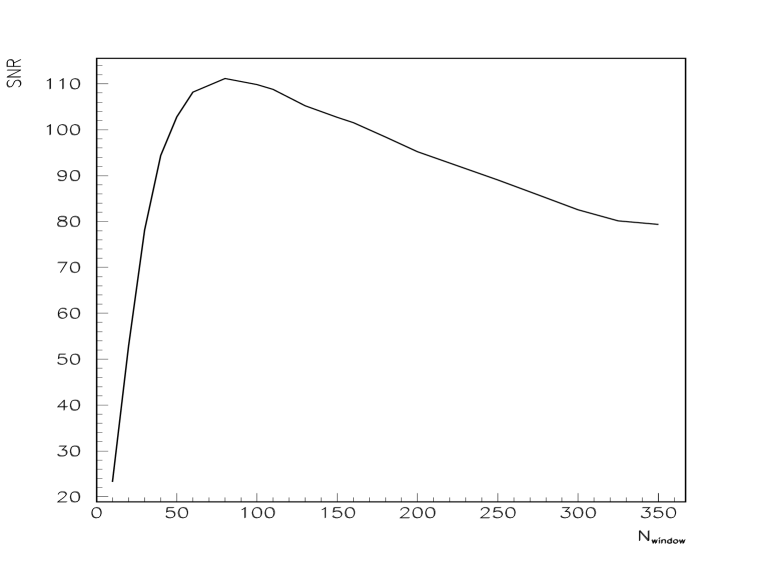
FIG. 3.: SNR $X_{a}$ for a Gaussian burst signal of width $\Delta=$0.5 ms as a function of the analysis window size $N$. The maximum SNR is obtained for $N\simeq 7\Delta$.

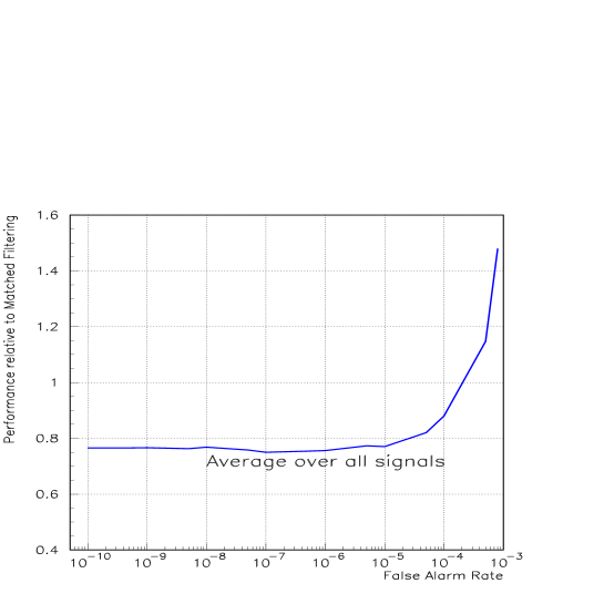
FIG. 4.: Relative Performance of ALF (single-windowed) as a function of the False Alarm Rate, averaged over all the signals of the catalogue.

FIG. 5.: Performance of Single-Windowing Filters Slope, Offset and ALF as a function of the window size. The error bars take into account the finite statistic of the waveforms taken from the Catalogue.

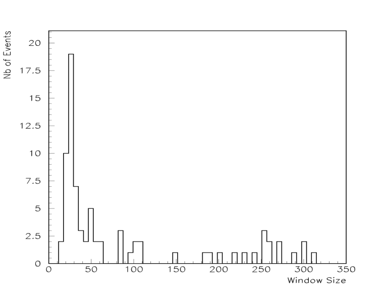
FIG. 6.: Distribution of Window Sizes (in number of samplings at 20 kHz) that give optimal performances for ALF. Short duration windows (up to about 100 bins, i.e 5 ms) are clearly preferred.

FIG. 7.: Detection efficiency of the filters as a function of the distances of the source.The distances are normalised to the optimal distances of detection for each signal and the efficiency is averaged over all the signals of the Zwerger and Müller catalogue.

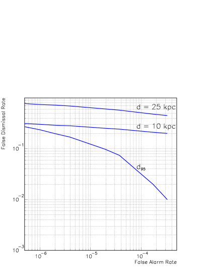
FIG. 8.: False Dismissal Rate as a function of False Alarm Rate for all signals located at 10 kpc and 25 kpc. The curve labelled $d_{95}$ concerns signals located at a distance such that for ALF (with 5 different window sizes), $\epsilon_{ALF}\simeq 95\%$ (for $\kappa_{0}\sim 10^{-6}$), that is, a different distance for each signal. Dashed lines represent 25 $\%$, 50 $\%$ and 75 $\%$ false dismissal rate.

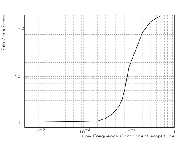
FIG. 9.: False Alarms Excess as a function of the amplitude of a low frequency component (here 0.6 Hz) added to white noise. This excess is the quantity (Effective Number of False alarms)/(Allowed Number of False Alarms). The amplitud8e is measured relatively to the standard deviation of the noise. In this figure, the amplitude $A_{10\%}$ represents a false alarm excess of $1.1$.

REFERENCES

- [1] A. Abramovici, W.E. Althouse, R.W.P. Drever, Y. Gürsel, S. Kawamura, F.J. Raab, D. Shoemaker, L. Sievers, R.E. Spero, K.S. Thorne, R.E. Vogt, R. Weiss, S.E. Whitcomb and M.E. Zucker, Science 256, 325 (1992).
- [2] B. Caron et al. “The VIRGO Interferometer for Gravitational Wave Detection”, Nucl. Phys. B (Proc. Sup.) 54B, 167 (1997).
- [3] K. Danzmann et al., “GEO 600, a 600 m laser interferometric gravitational wave antenna” in “Gravitational wave experiments”, edited by E. Coccia, G. Pizzella and F. Ronga (World Scientific, Singapore, 1995).
- [4] K. Kuroda, “Status of TAMA” in “Gravitational waves : sources and detectors”, edited by I. Ciufolini and F. Fidecaro (World Scientific, Singapore, 1997).
- [5] B.F. Schutz, “Data processing, analysis and storage for interferometric antennas”, in “The detection of gravitational waves”, edited by D.G. Blair (Cambridge University Press, Cambridge, 1991).
- [6] R. Mönchmeyer, G. Schäfer, E. Müller and R.E. Kates, Astron. Astrophys. 246, 417 (1991).
- [7] S. Bonazzola and J.-A. Marck, Astron. Astrophys. 267, 623 (1993).
- [8] T. Zwerger and E. Müller, Astron. Astrophys. 320, 209 (1997).
- [9] M. Rampp, E. Müller and M. Ruffert, Astron. Astrophys. 332, 969 (1998).
- [10] R.F. Stark and T. Piran, Phys. Rev. Lett. 55, 891 (1985).
- [11] K. Oohara and T. Nakamura, “Coalescences of binary neutron stars” in “Relativistic gravitation and gravitational waves”, edited by J.-A. Marck and J.-P. Lasota (Cambridge University Press, Cambridge, 1997).
- [12] M. Ruffert and H.-Th. Janka, Astron. Astrophys. 338, 535 (1998).
- [13] H.-T. Janka, T. Eberl, M. Ruffert and C.L. Fryer, Astrophys. J. 527, L39 (1999).
- [14] L.S. Finn, S.D. Mohanty and J.D. Romano, Phys. Rev. D 60, 121101 (1999).
- [15] The Binary Black Hole Grand Challenge Alliance’s web page is located at http://www.npac.syr.edu/projects/bh/ .
- [16] G. Khanna, R. Gleiser, R. Price and J. Pullin, New J.Phys.2, 3 (2000).
- [17] E.E. Flanagan and S.A Hughes, Phys. Rev. D 57, 4535 (1998).
- [18] W. G. Anderson, P.R. Brady, J.D.E Creighton and E.E. Flanagan, “ A power filter for the detection of burst sources of gravitational radiation in interferometric detectors” in the proceedings of the Gravitational Wave Data Analysis Workshop (Roma, 1999), gr-qc/0001044.
- [19] W. G. Anderson, P.R. Brady, J.D.E Creighton and E.E. Flanagan, “An excess power statistic for detection of burst sources of gravitational radiation”, gr-qc/0008066
- [20] N. Arnaud, F. Cavalier, M. Davier and P. Hello, Phys. Rev. D 59, 082002 (1999).
- [21] W. G. Anderson and R. Balasubramanian, Phys. Rev. D 60, 102001 (1999).
- [22] S. D. Mohanty, “A robust test for detecting non-stationarity in data from gravitational wave detectors”, preprint gr-qc/9910027, accepted for publication in Phys. Rev. D.
- [23] J.D.E Creighton, Phys. Rev. D 60, 021101 (1999).
- [24] Y. Gürsel and M. Tinto, Phys. Rev. D 40, 3884 (1989).
- [25] N. Arnaud, F. Cavalier, M. Davier, P. Hello and T. Pradier, ”Triggers for the detection of gravitational wave bursts”, to appear in the proceedings of the XXXIVth Rencontres de Moriond on ”Gravitational Waves and Experimental Gravity” (les Arcs, Jan.99), gr-qc/9903035.
- [26] T. Pradier, N. Arnaud, M.-A. Bizouard, F. Cavalier, M. Davier and P. Hello, “About the detection of gravitational wave bursts”, in the proceedings of the Gravitational Wave Data Analysis Workshop (Roma, 1999), gr-qc/0001062.
- [27] The factor forgotten in [20] has been here corrected for.
- [28] The “official” VIRGO sensitivity curve is available at : http://www.pg.infn.it/virgo/presentation.htm
- [29] M.Beccaria, E. Cuoco and G. Curci, “Adaptive Identification of VIRGO-like noise spectrum” in the proceedings of the Second Edoardo Amaldi Conference on Gravitational Waves, Edoardo Amaldi Foundation series Vol.IV, edited by E. Coccia, G. Pizzela and G. Veneziano (World Scientific, 1998).
- [30] E. Cuoco, “Whitening of noise power spectrum”, Virgo note VIR-NOT-FIR 1390 145 (2000), unpublished.
- [31] G.A. Prodi et al., “Initial operation of the International Gravitational Event Collaboration”, in the proceedings of the Gravitational Wave Data Analysis Workshop (Roma, 1999), astro-ph/0003106. See also http://igec.lnl.infn.it
- [32] http://www.mpa-garching.mpg.de/ewald/GRAV/grav.html
- [33] A. Buonanno and T. Damour, “Transition from inspiral to plunge in binary black hole coalescences”, preprint gr-qc/0001013 (2000).
- [34] F. Cavalier, M. Davier, P. Hello and T. Pradier, “Triggers for the detection of impulsive sources of gravitational waves”, Virgo note VIR-NOT-LAL-1390 128 (1999), unpublished. T. Pradier et al. “Improved slope filters for detecting bursts”, VIR-NOT-LAL-1390 160 (2000), unpublished.
- [35] F. Echeverria, Phys. Rev. D 40, 3194 (1989).