Aperture synthesis for gravitational-wave data analysis: Deterministic Sources

Lee Samuel Finn Center for Gravitational Physics and Astronomythanks: Also Department of Physics and Department of Astronomy and Astrophysics; e-mail LSF5@PSU.Edu., The Pennsylvania State University, University Park PA 16802
Abstract

Gravitational wave detectors now under construction are sensitive to the phase of the incident gravitational waves. Correspondingly, the signals from the different detectors can be combined, in the analysis, to simulate a single detector of greater amplitude and directional sensitivity: in short, aperture synthesis. Here we consider the problem of aperture synthesis in the special case of a search for a source whose waveform is known in detail: e.g., compact binary inspiral. We derive the likelihood function for joint output of several detectors as a function of the parameters that describe the signal and find the optimal matched filter for the detection of the known signal. Our results allow for the presence of noise that is correlated between the several detectors. While their derivation is specialized to the case of Gaussian noise we show that the results obtained are, in fact, appropriate in a well-defined, information-theoretic sense even when the noise is non-Gaussian in character.

The analysis described here stands in distinction to “coincidence analyses”, wherein the data from each of several detectors is studied in isolation to produce a list of candidate events, which are then compared to search for coincidences that might indicate common origin in a gravitational wave signal. We compare these two analyses — optimal filtering and coincidence — in a series of numerical examples, showing that the optimal filtering analysis always yields a greater detection efficiency for given false alarm rate, even when the detector noise is strongly non-Gaussian.

I Introduction

Several large interferometric gravitational wave detectors [1, 2, 3] will soon be operating, perhaps to be joined by several as or more sensitive acoustic resonant detectors [4, 5, 6] in the years to come. There are several reasons for wanting to combine, in some way the, the data from these detectors in order to draw inferences about the presence of a signal or the parameters that characterize it: for example, observations of a signal with several detectors increase the degree of confidence in the detection and characterization of a signal, and the use of several geographically separated detectors can allow one to disentangle source parameters (e.g., sky position, polarization) that are degenerate when observed in a single detector.

The signal response of both interferometric and acoustic detectors is sensitive to the phase of the incident gravitational waves; consequently, we have the opportunity to combine interfere the response of several detectors, synthesizing a single, effectively larger and more directionally sensitive detector: in short, aperture synthesis. Here we describe a likelihood-based analysis for the detection of a signal of known, parameterized form in the joint output of a network of detectors. Such an analysis makes the most effective use of the information available from each detector, in exactly the same sense that optimal filter described in [7, 8, 9] is best-suited for detecting or characterizing radiation incident on a single detector.

The analysis described here stands in contrast to a “coincidence” analysis, whereby “events” are identified independently in separate detectors and these independent lists of events are later brought together and compared for coincidences [10, 11]. The key difference between the two analyses is their sensitivity to inter-detector correlations. The response of a network of gravitational wave detectors to an incident plane wave is phase coherent. This phase coherence is captured in the likelihood function describing the output of a network of detectors; however, it is absent in a coincidence analysis. This leads the likelihood analysis to have an increased detection efficiency for a given false alarm rate when compared to a coincidence analysis searching for the same signals and based on the same detector output.

We demonstrate this directly in a set of three numerical examples, based on a network consisting of two separated detectors. In each example we search for a signal of known waveform arriving at an arbitrary time and from an arbitrary direction. Two different search algorithms are investigated. The first is based on the maximum of the likelihood of the joint detector output; the second is based on the analysis of coincidences between the optimally filtered output of each detector, considered separately. The three examples differ in the character of the simulated noise: in the examples the noise is either Normal, strongly leptokurtic or strongly platykurtic. In all cases the likelihood analysis described here gives a substantially larger detection efficiency for a fixed false alarm rate.

Most previous work on multi-detector gravitational wave data analysis has focused on coincidence analyses or variations on coincidence analyses [10, 11, 12] that occur separately at each detector. The work described here parallels recent, independent work by Bose and collaborators [13, 14]. It goes beyond that work by allowing from the beginning detectors that are not coincident and accommodating the possibility that the noise between pairs of detectors may be correlated.

Section II introduces terminology and nomenclature used throughout this work. In section III the likelihood function for the joint output of a set of gravitational wave detectors is derived. The form derived here is exact when the detector noise is Normal; however, we show that it is also the best choice (in the sense of making the least additional assumptions about the noise statistics) when only the detector cross- and auto-correlations are known. In section IV we describe and present the results of several numerical examples, meant to compare likelihood and coincidence-based approaches to data analysis. Finally, in section V we summarize our conclusions.

II Nomenclature

A Continuous and discrete time signals

While gravitational wave detectors are analog devices, the detector output, including diagnostic channels containing physical and environmental monitors, will be quantized in magnitude and sampled discretely in time. Data analysis will operate exclusively with this discrete time series.

Properly handled, quantization of the continuous amplitude contributes a small, white, additive component to the detector noise [15, Chapter 3.7.3], which we will not discuss further here.

When certain other conditions hold, the continuous in time and discretely sampled time series are equivalent and fully interchangeable. In this paper we have occasion to refer to both discrete and continuous time representations of the same underlying process. To distinguish between these two representations, we refer to the continuous time representation of the process $x$ by $x(t)$, where $t$ denotes continuous time, and the discrete time representation of the same process by $x[k]$, where integer $k$ denotes the sample number.

B Scalar-, vector- and matrix-valued functions and sequences

For our purposes, the output of a single gravitational-wave detector is a real, scalar-valued time series. An important purpose of this paper is to discuss data analysis for a gravitational-wave receiver, by which we mean a logical collection of detectors. The output of a receiver is a vector-valued time series. The elements of the vector at any given sample are the detector outputs at the corresponding moment of time.

In this paper we will have occasion to refer to scalar-, vector- and matrix-valued time series. To distinguish between these different cases, we use a lowercase italic face (as in $a$) to denote scalars or scalar-valued sequences, a lowercase bold-italic face (as in $\textstyle a$) to denote vectors or vector sequences, and an uppercase bold-italic face (as in $\textstyle A$) to denote matrices or matrix-valued sequences (functions).

C Discrete Fourier transform

Many different conventions for the discrete Fourier transform (DFT) can be found in the literature. We adopt the conventions described in this section. If you compare the notation used here with other conventions found in the literature, it will be to your advantage to pay careful attention to the normalization, index range of the input and output sequences, and sign convention of the transform kernel.

Suppose that $x[k]$ is a sequence of coefficients of length $N$, with initial index $k_{0}$. The DFT $\widetilde{x}[k]$ of the sequence $x[k]$ is the periodic sequence given by

$$\widetilde{x}[j]=\sum_{k=k_{0}}^{k_{0}+N-1}x[k]\omega_{N}^{jk},$$ (2)

where

$$\omega_{N}\equiv\exp(-2\pi i/N)$$ (3)

is the $N^{\text{th}}$ root of unity. (Note our use of the engineering convention for the transformation kernel.)

The kernel of the transform, $\omega_{N}^{jk}$, satisfies an orthogonality relationship,

$$\delta_{kl}={1\over N}\sum_{n=0}^{N-1}\omega_{N}^{kn}\omega_{N}^{-nl}$$ (4)

as $k$ and $l$ run from 00 to $N-1$; consequently, the DFT is invertible. The inverse DFT (IDFT) is given by

$$\check{x}[n]={1\over N}\sum_{k=0}^{N-1}\widetilde{x}[k]\omega_{N}^{-nk}.$$ (5)

Note that the IDFT is also a periodic sequence. In particular, if $\tilde{x}[k]$ is the DFT of a sequence $x[j]$, then $\check{x}[k]$ is the periodic extension of $x[j]$.

A wealth of useful results and insights into the DFT/IDFT pair are found in [16]; additionally, [15] discusses the use of the DFT/IDFT pair in digital signal processing.

D Terminology

A receiver is a collection of one or more individual gravitational-wave detectors whose output is analyzed collectively to draw a single set of inferences regarding the presence and properties of radiation sources. The elements of the receiver are the detectors, which need not be co-located, co-oriented, or of identical design, sensitivity or bandwidth. For example, a single receiver might consist of

  • $\bullet$

    the three LIGO interferometers (a 4 Km and a 2 Km interferometer in Washington State, USA, and a 4 Km interferometer interferometer in Louisiana, USA) [2],

  • $\bullet$

    the Virgo interferometer (located in Pisa, Italy [3]),

  • $\bullet$

    the GEO-600 interferometer (located in Hannover, Germany [1]),

  • $\bullet$

    the TAMA-300 interferometer (located in Tokyo, Japan [17]),

  • $\bullet$

    the ALLEGRO detector (a resonant mass detector located in Louisiana [18]),

  • $\bullet$

    the AURIGA detector (a resonant mass detector located in Padua [19]),

  • $\bullet$

    the Explorer detector (a resonant mass detector located in Frascati [20]), and

  • $\bullet$

    the Nautilus detector (a resonant mass detector located in Geneva [21]).

A gravitational-wave receiver is thus a logical grouping of gravitational-wave detectors.

The output of detector $\alpha$ is the scalar-valued time-series $g_{\alpha}$. The output $\textstyle g$ of a receiver composed of several detectors $\alpha,\ldots,\omega$ is the direct sum of the output of the individual detectors:

$$\mathchoice{{\hbox{\boldmath$\displaystyle g$}}}{{\hbox{\boldmath$\textstyle g$}}}{{\hbox{\boldmath$\scriptstyle g$}}}{{\hbox{\boldmath$\scriptscriptstyle g$}}}=g_{\alpha}\oplus\cdots\oplus g_{\omega}.$$ (6)

The receiver response $\textstyle m$ to an incident gravitational-wave $\textstyle h$ depends on parameters $\textstyle\theta$ that reflect both the intrinsic properties of the source and the relationship of the source to the receiver (i.e., distance and orientation). For example, if the source is a stochastic gravitational-wave signal, then $\textstyle\theta$ describes the signal spectrum and anisotropy; alternatively, if the source is an inspiraling compact binary system, then $\textstyle\theta$ describes the binary’s component masses, spins and orbital characteristics. In this paper I discuss analysis for deterministic signals: i.e., signals like those that arise from binary inspiral or rapidly rotating non-axisymmetric neutron stars, whose waveform can be accurately described in terms of a small number of parameters that characterize the source and its orientation with respect to the detector.

III The Likelihood Function

A Introduction

Let $H_{0}$ and $H_{\mathchoice{{\hbox{\boldmath$\displaystyle\theta$}}}{{\hbox{\boldmath$\textstyle\theta$}}}{{\hbox{\boldmath$\scriptstyle\theta$}}}{{\hbox{\boldmath$\scriptscriptstyle\theta$}}}}$ denote alternative, exclusive hypotheses regarding the presence or absence of a signal:

$\displaystyle H_{0}$ $\displaystyle=$ $\displaystyle\left(\begin{tabular}[]{l}proposition that the receiver\\ output consists only of noise\end{tabular}\right),$ (10)
$\displaystyle H_{\mathchoice{{\hbox{\boldmath$\displaystyle\theta$}}}{{\hbox{\boldmath$\textstyle\theta$}}}{{\hbox{\boldmath$\scriptstyle\theta$}}}{{\hbox{\boldmath$\scriptscriptstyle\theta$}}}}$ $\displaystyle=$ $\displaystyle\left(\begin{tabular}[]{l}{proposition that the receiver}\\ {output consists of signal $\mathchoice{{\hbox{\boldmath$\displaystyle s$}}}{{\hbox{\boldmath$\textstyle s$}}}{{\hbox{\boldmath$\scriptstyle s$}}}{{\hbox{\boldmath$\scriptscriptstyle s$}}}_{\mathchoice{{\hbox{\boldmath$\displaystyle\theta$}}}{{\hbox{\boldmath$\textstyle\theta$}}}{{\hbox{\boldmath$\scriptstyle\theta$}}}{{\hbox{\boldmath$\scriptscriptstyle\theta$}}}}$}\\ {superposed with receiver noise}\end{tabular}\right)$ (14)

where $\textstyle\theta$ represents a set of parameters that differentiate signals in the detector: for example, if the signal is from an inspiraling binary neutron star or black hole system, the parameters include the component masses and the source distance from and orientation with respect to the receiver. In this section we derive the likelihood function $\Lambda(\mathchoice{{\hbox{\boldmath$\displaystyle g$}}}{{\hbox{\boldmath$\textstyle g$}}}{{\hbox{\boldmath$\scriptstyle g$}}}{{\hbox{\boldmath$\scriptscriptstyle g$}}}|\mathchoice{{\hbox{\boldmath$\displaystyle\theta$}}}{{\hbox{\boldmath$\textstyle\theta$}}}{{\hbox{\boldmath$\scriptstyle\theta$}}}{{\hbox{\boldmath$\scriptscriptstyle\theta$}}})$, describing the probability that $\textstyle g$ is observed under the hypothesis $H_{\mathchoice{{\hbox{\boldmath$\displaystyle\theta$}}}{{\hbox{\boldmath$\textstyle\theta$}}}{{\hbox{\boldmath$\scriptstyle\theta$}}}{{\hbox{\boldmath$\scriptscriptstyle\theta$}}}}$.

Why the likelihood function? Recall that the likelihood is any function that, viewed as a function of $\textstyle\theta$, is proportional to $P(\mathchoice{{\hbox{\boldmath$\displaystyle g$}}}{{\hbox{\boldmath$\textstyle g$}}}{{\hbox{\boldmath$\scriptstyle g$}}}{{\hbox{\boldmath$\scriptscriptstyle g$}}}|H_{\mathchoice{{\hbox{\boldmath$\displaystyle\theta$}}}{{\hbox{\boldmath$\textstyle\theta$}}}{{\hbox{\boldmath$\scriptstyle\theta$}}}{{\hbox{\boldmath$\scriptscriptstyle\theta$}}}})$, the probability of observing $\textstyle g$ given the fixed hypothesis $H_{\mathchoice{{\hbox{\boldmath$\displaystyle\theta$}}}{{\hbox{\boldmath$\textstyle\theta$}}}{{\hbox{\boldmath$\scriptstyle\theta$}}}{{\hbox{\boldmath$\scriptscriptstyle\theta$}}}}$. In a Bayesian analysis, the goal is to determine or characterize $P(H_{\mathchoice{{\hbox{\boldmath$\displaystyle\theta$}}}{{\hbox{\boldmath$\textstyle\theta$}}}{{\hbox{\boldmath$\scriptstyle\theta$}}}{{\hbox{\boldmath$\scriptscriptstyle\theta$}}}}|\mathchoice{{\hbox{\boldmath$\displaystyle g$}}}{{\hbox{\boldmath$\textstyle g$}}}{{\hbox{\boldmath$\scriptstyle g$}}}{{\hbox{\boldmath$\scriptscriptstyle g$}}})$, the probability of the hypothesis given the observation. Through Bayes Theorem, this quantity is directly related to the likelihood. In frequentist statistical analysis the goal is to determine the improbability of observing $\textstyle g$ under the alternative hypotheses that the signal is absent or that it is present, or to establish confidence intervals — a range of hypotheses $H_{\mathchoice{{\hbox{\boldmath$\displaystyle\theta$}}}{{\hbox{\boldmath$\textstyle\theta$}}}{{\hbox{\boldmath$\scriptstyle\theta$}}}{{\hbox{\boldmath$\scriptscriptstyle\theta$}}}}$ for which the observation has, in a certain sense, high probability [22]. In either case the likelihood plays a central role and no other function of the observation and hypotheses offers the prospect of stronger statements.

In our derivation of the likelihood we assume that the noise in each detector is Gaussian and stationary. While the fundamental noise sources in gravitational wave detectors are all characterized by Gaussian-stationary statistics, the realities of an actual implementation — e.g., detector imperfections and environmental couplings — guarantee that the actual noise character will be neither Gaussian nor stationary. Characterizing the detector, which includes identifying instrumental and environmental artifacts in the “gravity-wave channel” and regressing or removing these artifacts to the greatest possible extent, is a necessary pre-requisite to the analysis of the data for gravitational waves. We assume here that these artifacts have already been dealt with as best possible, so that $\textstyle g$ contains no identifiable instrumental artifacts, transient or otherwise, and that the noise is stationary on timescales long compared to the duration of a signal.

Even so, the noise will remain non-Gaussian and non-stationary. As long as the evolution of the noise character is adiabatic — i.e., it varies only on timescales long compared to the signal duration and the time required to estimate the moments of the noise distribution — we can treat the noise as stationary on any important sub-interval. It is also an excellent approximation to treat the noise as Gaussian. To see why, focus on a stationary noise process but without any assumption on its distribution ${\cal P}(x)$. Suppose, by observations on the noise, we estimate its mean $\mu$ ($\overline{x}$) and variance $\sigma^{2}$ ($\overline{(x-\mu)^{2}}$). What probability distribution makes the least assumptions about the process while remaining consistent with this information? This information-theoretic question has a definite answer: it is the probability distribution $P(x|I)$ with maximum entropy, subject to the constraints on its mean and variance: i.e., the distribution $P(x|\mu,\sigma)$ that maximizes the functional

$\displaystyle I(P):=-\int_{-\infty}^{\infty}dx\;P(x|\mu,\sigma)\ln P(x|\mu,\sigma)-\lambda_{0}\int_{-\infty}^{\infty}dx\;P(x|\mu,\sigma)$ (16)
$\displaystyle-\lambda_{1}\int_{-\infty}^{\infty}dx\;x\,P(x|\mu,\sigma)-\lambda_{2}\int_{-\infty}^{\infty}dx\;(x-\mu)^{2}\,P(x|\mu,\sigma)$

where $\lambda_{0}$, $\lambda_{1}$ and $\lambda_{2}$ are the Lagrange multipliers corresponding to the constraints on the overall normalization of the probability, the mean and the variance. The solution to this variational problem is

$$P(x|I)={\exp\left[(x-\mu)^{2}/2\sigma^{2}\right]\over\sqrt{2\pi\sigma^{2}}},$$ (17)

i.e., the normal distribution. Similarly, if we have a correlated process known to us only through its mean and autocorrelation,

$$C[k-j]:=\overline{\left(x[j]-\mu\right)\left(x[k]-\mu\right)},$$ (18)

the distribution that makes the least assumptions about the process beyond these is the multivariate normal distribution

$$P\left(\left\{x[j]\right\}|\mu,C\right)={\exp\left[-{1\over 2}\sum_{j,k=0}^{N_{T}-1}\left(x[k]-\mu\right)\left|\left|\mathchoice{{\hbox{\boldmath$\displaystyle C$}}}{{\hbox{\boldmath$\textstyle C$}}}{{\hbox{\boldmath$\scriptstyle C$}}}{{\hbox{\boldmath$\scriptscriptstyle C$}}}^{-1}\right|\right|_{kl}\left(x[l]-\mu\right)\right]\over\sqrt{\left(2\pi\right)^{N_{T}}\text{det}||\mathchoice{{\hbox{\boldmath$\displaystyle C$}}}{{\hbox{\boldmath$\textstyle C$}}}{{\hbox{\boldmath$\scriptstyle C$}}}{{\hbox{\boldmath$\scriptscriptstyle C$}}}||}},$$ (19)

where $\left\{x[k]\right\}$ is a set of $N_{T}$ samples indexed by the sample times and the matrix $\textstyle C$ has components

$$\left|\left|\mathchoice{{\hbox{\boldmath$\displaystyle C$}}}{{\hbox{\boldmath$\textstyle C$}}}{{\hbox{\boldmath$\scriptstyle C$}}}{{\hbox{\boldmath$\scriptscriptstyle C$}}}\right|\right|_{jk}:=C[k-j].$$ (20)

Thus, modeling (correlated) noise as arising from a (multi-variate) Normal distribution is simultaneously the best and most conservative assumption that one can make when all one knows is the noise mean and (co-)variance.

Put another way, if our only knowledge of the noise character is its first and second moments (i.e., mean and correlation function or power spectrum) then treating the noise as anything but Normally distributed is to assume more than we actually know and, consequently, would lead us to overstate the accuracy of any conclusions we reach.

We choose a particular normalization of the likelihood function, as the ratio of $P(\mathchoice{{\hbox{\boldmath$\displaystyle g$}}}{{\hbox{\boldmath$\textstyle g$}}}{{\hbox{\boldmath$\scriptstyle g$}}}{{\hbox{\boldmath$\scriptscriptstyle g$}}}|\mathchoice{{\hbox{\boldmath$\displaystyle\theta$}}}{{\hbox{\boldmath$\textstyle\theta$}}}{{\hbox{\boldmath$\scriptstyle\theta$}}}{{\hbox{\boldmath$\scriptscriptstyle\theta$}}})$ to the probability that $\textstyle g$ arises from detector noise alone. The signal is assumed to be a plane gravitational wave incident on the detector array, so that the detectors respond to the signal coherently. If the hypothesized signal is characterized by parameters $\textstyle\theta$ (e.g., binary system chirp mass, orientation, distance, etc.) then we denote the likelihood function $\Lambda(\mathchoice{{\hbox{\boldmath$\displaystyle g$}}}{{\hbox{\boldmath$\textstyle g$}}}{{\hbox{\boldmath$\scriptstyle g$}}}{{\hbox{\boldmath$\scriptscriptstyle g$}}}|\mathchoice{{\hbox{\boldmath$\displaystyle\theta$}}}{{\hbox{\boldmath$\textstyle\theta$}}}{{\hbox{\boldmath$\scriptstyle\theta$}}}{{\hbox{\boldmath$\scriptscriptstyle\theta$}}})$ and regard it, for fixed receiver output $\textstyle g$, as a function of the signal parameterization $\textstyle\theta$.

The derivation of $\Lambda(\mathchoice{{\hbox{\boldmath$\displaystyle g$}}}{{\hbox{\boldmath$\textstyle g$}}}{{\hbox{\boldmath$\scriptstyle g$}}}{{\hbox{\boldmath$\scriptscriptstyle g$}}}|{\mathchoice{{\hbox{\boldmath$\displaystyle\theta$}}}{{\hbox{\boldmath$\textstyle\theta$}}}{{\hbox{\boldmath$\scriptstyle\theta$}}}{{\hbox{\boldmath$\scriptscriptstyle\theta$}}}})$ for a deterministic signal in a multi-detector receiver parallels closely the derivation of $\Lambda(g|{\mathchoice{{\hbox{\boldmath$\displaystyle\theta$}}}{{\hbox{\boldmath$\textstyle\theta$}}}{{\hbox{\boldmath$\scriptstyle\theta$}}}{{\hbox{\boldmath$\scriptscriptstyle\theta$}}}})$ given in [7, §II] for a single-detector receiver; however, in the generalization several new elements arise and are discussed here for the first time.

In section III B we walk through the construction of $P(\mathchoice{{\hbox{\boldmath$\displaystyle g$}}}{{\hbox{\boldmath$\textstyle g$}}}{{\hbox{\boldmath$\scriptstyle g$}}}{{\hbox{\boldmath$\scriptscriptstyle g$}}}|H_{0},{\cal I})$, the probability of observing $\textstyle g$ in the absence of any signal. Evaluation of $P(\mathchoice{{\hbox{\boldmath$\displaystyle g$}}}{{\hbox{\boldmath$\textstyle g$}}}{{\hbox{\boldmath$\scriptstyle g$}}}{{\hbox{\boldmath$\scriptscriptstyle g$}}}|H_{\mathchoice{{\hbox{\boldmath$\displaystyle\theta$}}}{{\hbox{\boldmath$\textstyle\theta$}}}{{\hbox{\boldmath$\scriptstyle\theta$}}}{{\hbox{\boldmath$\scriptscriptstyle\theta$}}}},{\cal I})$ (the probability of observing $\textstyle g$ when the signal characterized by $\textstyle\theta$ is present) and the likelihood function itself proceed much more quickly in section III C. In section III D we describe a detection test based solely on the maximum of the likelihood and identify the signal-to-noise ratio with the maximum of $\ln\Lambda$ over $\textstyle\theta$. In section III E we discuss how the likelihood function can be evaluated quickly and efficiently, which is critical to its use in real data analysis.

B Probability that $\textstyle g$ is receiver noise

Central to the evaluation of $\Lambda(\mathchoice{{\hbox{\boldmath$\displaystyle g$}}}{{\hbox{\boldmath$\textstyle g$}}}{{\hbox{\boldmath$\scriptstyle g$}}}{{\hbox{\boldmath$\scriptscriptstyle g$}}}|\mathchoice{{\hbox{\boldmath$\displaystyle\theta$}}}{{\hbox{\boldmath$\textstyle\theta$}}}{{\hbox{\boldmath$\scriptstyle\theta$}}}{{\hbox{\boldmath$\scriptscriptstyle\theta$}}})$ is the evaluation of $P(\mathchoice{{\hbox{\boldmath$\displaystyle g$}}}{{\hbox{\boldmath$\textstyle g$}}}{{\hbox{\boldmath$\scriptstyle g$}}}{{\hbox{\boldmath$\scriptscriptstyle g$}}}|H_{0},{\cal I})$, the probability that the receiver output $\textstyle g$ is an example of receiver noise $\textstyle n$. (Here $\cal I$ denotes other, unenumerated conditions.) The formulation of this probability density for a single detector (scalar-valued time series $g$) was discussed in [7]; in this section we review that discussion, setting the stage for our treatment of the more general problem of a multi-channel receiver (vector-valued $\textstyle g$).

1 Single-channel time series

Focus attention first on the single-channel output of a single detector. When the detector noise is Gaussian and stationary, any single sample $n[j]$ of detector noise is normally distributed with a mean and variance independent of when the sample was taken. Without loss of generality we can assume that the ensemble mean $\overline{{n}}$ vanishes, in which case the probability that a sample $g[j]$ of detector output is a sample of detector noise is

$$P(g[j]|H_{0},{\cal I})={\exp\left[-g[j]^{2}/2\sigma^{2}\right]\over\sqrt{2\pi\sigma^{2}}}.$$ (22)

The variance $\sigma^{2}$ of the distribution is the ensemble average of the square of the detector noise:

$$\sigma^{2}=\overline{n^{2}}.$$ (23)

Equation 22 holds true for each sample $g[j]$; consequently, the joint probability that the length $N_{T}$ sequence $g$ is a sample of detector noise is given by the multivariate Gaussian distribution

$$P(g|H_{0},{\cal I})={\exp\left[-{1\over 2}\sum_{j,k=0}^{N_{T}-1}g[j]\left|\left|\mathchoice{{\hbox{\boldmath$\displaystyle C$}}}{{\hbox{\boldmath$\textstyle C$}}}{{\hbox{\boldmath$\scriptstyle C$}}}{{\hbox{\boldmath$\scriptscriptstyle C$}}}^{-1}\right|\right|_{jk}g[k]\right]\over\sqrt{\left(2\pi\right)^{N_{T}}\det\left|\left|\mathchoice{{\hbox{\boldmath$\displaystyle C$}}}{{\hbox{\boldmath$\textstyle C$}}}{{\hbox{\boldmath$\scriptstyle C$}}}{{\hbox{\boldmath$\scriptscriptstyle C$}}}\right|\right|}}$$ (24)

In place of the variance $\sigma^{2}$ that appears in the exponent of equation 22 is the matrix $\mathchoice{{\hbox{\boldmath$\displaystyle C$}}}{{\hbox{\boldmath$\textstyle C$}}}{{\hbox{\boldmath$\scriptstyle C$}}}{{\hbox{\boldmath$\scriptscriptstyle C$}}}^{{-1}}$. As $P(g|H_{0},{\cal I})$ is a probability so $\mathchoice{{\hbox{\boldmath$\displaystyle C$}}}{{\hbox{\boldmath$\textstyle C$}}}{{\hbox{\boldmath$\scriptstyle C$}}}{{\hbox{\boldmath$\scriptscriptstyle C$}}}^{{-1}}$ is positive definite and invertible. The matrix $\textstyle C$ gives the covariance of the noise process: it is equal to the ensemble average of the product of the detector noise at different samples:

$$\overline{{n}[j]{n}[k]}=\left|\left|\mathchoice{{\hbox{\boldmath$\displaystyle C$}}}{{\hbox{\boldmath$\textstyle C$}}}{{\hbox{\boldmath$\scriptstyle C$}}}{{\hbox{\boldmath$\scriptscriptstyle C$}}}\right|\right|_{jk}.$$ (25)

Since the detector noise is also assumed to be stationary, $\left|\left|\mathchoice{{\hbox{\boldmath$\displaystyle C$}}}{{\hbox{\boldmath$\textstyle C$}}}{{\hbox{\boldmath$\scriptstyle C$}}}{{\hbox{\boldmath$\scriptscriptstyle C$}}}\right|\right|_{jk}$ can depend only on the difference $j-k$; correspondingly, $\textstyle C$ is constant on its diagonals: i.e., it is a Toeplitz matrix. Since $\textstyle C$ is Toeplitz it is characterized completely by the scalar sequence $c[k]$ of length $2N_{T}-1$ whose elements are the first row and column of $\textstyle C$:

$$c[j-k]:=\left|\left|\mathchoice{{\hbox{\boldmath$\displaystyle C$}}}{{\hbox{\boldmath$\textstyle C$}}}{{\hbox{\boldmath$\scriptstyle C$}}}{{\hbox{\boldmath$\scriptscriptstyle C$}}}\right|\right|_{jk}.$$ (26)

This sequence is the noise autocorrelation. The DFT of $c[k]$ is related to the noise power spectral density.

2 Multi-channel time series

Now consider a receiver consisting of $N_{D}$ component detectors, where the receiver output is an $N_{D}$-dimensional time series. Without loss of generality assume that, while the different detectors that comprise the receiver may be sampled at different rates, all the detector outputs have been resampled so that the interval between samples in all detector data streams is $\Delta t$. The receiver output $\textstyle g$ is a multi-channel time series: a vector-valued sequence consisting of the direct sum of the output $g_{\alpha}$ of the individual detectors. Similarly, the receiver noise $\textstyle n$ is the direct sum of the noise contributions $n_{\alpha}$ to the output of the $N_{D}$ detectors:

$\displaystyle\mathchoice{{\hbox{\boldmath$\displaystyle g$}}}{{\hbox{\boldmath$\textstyle g$}}}{{\hbox{\boldmath$\scriptstyle g$}}}{{\hbox{\boldmath$\scriptscriptstyle g$}}}[k]$ $\displaystyle:=$ $\displaystyle g_{1}[k]\oplus\cdots\oplus g_{N_{D}}[k]$ (28)
$\displaystyle\mathchoice{{\hbox{\boldmath$\displaystyle n$}}}{{\hbox{\boldmath$\textstyle n$}}}{{\hbox{\boldmath$\scriptstyle n$}}}{{\hbox{\boldmath$\scriptscriptstyle n$}}}[k]$ $\displaystyle:=$ $\displaystyle n_{1}[k]\oplus\cdots\oplus n_{N_{D}}[k].$ (29)

Focus attention on a single sample of the receiver output: i.e., the vector $\mathchoice{{\hbox{\boldmath$\displaystyle g$}}}{{\hbox{\boldmath$\textstyle g$}}}{{\hbox{\boldmath$\scriptstyle g$}}}{{\hbox{\boldmath$\scriptscriptstyle g$}}}[j]$. Since the receiver noise is Gaussian and stationary, the probability that sample $\mathchoice{{\hbox{\boldmath$\displaystyle g$}}}{{\hbox{\boldmath$\textstyle g$}}}{{\hbox{\boldmath$\scriptstyle g$}}}{{\hbox{\boldmath$\scriptscriptstyle g$}}}[j]$ is a sample of receiver noise $\textstyle n$ is given by the multivariate Gaussian

$$P(\mathchoice{{\hbox{\boldmath$\displaystyle g$}}}{{\hbox{\boldmath$\textstyle g$}}}{{\hbox{\boldmath$\scriptstyle g$}}}{{\hbox{\boldmath$\scriptscriptstyle g$}}}[j]|H_{0},{\cal I})={\exp\left[-{1\over 2}\mathchoice{{\hbox{\boldmath$\displaystyle g$}}}{{\hbox{\boldmath$\textstyle g$}}}{{\hbox{\boldmath$\scriptstyle g$}}}{{\hbox{\boldmath$\scriptscriptstyle g$}}}[j]\cdot\mathchoice{{\hbox{\boldmath$\displaystyle C$}}}{{\hbox{\boldmath$\textstyle C$}}}{{\hbox{\boldmath$\scriptstyle C$}}}{{\hbox{\boldmath$\scriptscriptstyle C$}}}[0]^{-1}\cdot\mathchoice{{\hbox{\boldmath$\displaystyle g$}}}{{\hbox{\boldmath$\textstyle g$}}}{{\hbox{\boldmath$\scriptstyle g$}}}{{\hbox{\boldmath$\scriptscriptstyle g$}}}[j]\right]\over\sqrt{\left(2\pi\right)^{N_{D}}\det\left|\left|\mathchoice{{\hbox{\boldmath$\displaystyle C$}}}{{\hbox{\boldmath$\textstyle C$}}}{{\hbox{\boldmath$\scriptstyle C$}}}{{\hbox{\boldmath$\scriptscriptstyle C$}}}[0]\right|\right|}}$$ (31)

where the matrix $\mathchoice{{\hbox{\boldmath$\displaystyle C$}}}{{\hbox{\boldmath$\textstyle C$}}}{{\hbox{\boldmath$\scriptstyle C$}}}{{\hbox{\boldmath$\scriptscriptstyle C$}}}[0]$ is the ensemble average of the outer product of a sample of receiver noise with itself:

$$\mathchoice{{\hbox{\boldmath$\displaystyle C$}}}{{\hbox{\boldmath$\textstyle C$}}}{{\hbox{\boldmath$\scriptstyle C$}}}{{\hbox{\boldmath$\scriptscriptstyle C$}}}[0]=\overline{\mathchoice{{\hbox{\boldmath$\displaystyle n$}}}{{\hbox{\boldmath$\textstyle n$}}}{{\hbox{\boldmath$\scriptstyle n$}}}{{\hbox{\boldmath$\scriptscriptstyle n$}}}[j]\otimes\mathchoice{{\hbox{\boldmath$\displaystyle n$}}}{{\hbox{\boldmath$\textstyle n$}}}{{\hbox{\boldmath$\scriptstyle n$}}}{{\hbox{\boldmath$\scriptscriptstyle n$}}}[j]}.$$ (32)

As suggested by the selection index $[0]$, $\mathchoice{{\hbox{\boldmath$\displaystyle C$}}}{{\hbox{\boldmath$\textstyle C$}}}{{\hbox{\boldmath$\scriptstyle C$}}}{{\hbox{\boldmath$\scriptscriptstyle C$}}}[0]$ is one element of a sequence of correlation matrices. Each element of this sequences arises from the ensemble average of the outer product of receiver noise with itself at a different time. Since the receiver noise is stationary, the ensemble average depends only on the time difference; consequently,

$$\mathchoice{{\hbox{\boldmath$\displaystyle C$}}}{{\hbox{\boldmath$\textstyle C$}}}{{\hbox{\boldmath$\scriptstyle C$}}}{{\hbox{\boldmath$\scriptscriptstyle C$}}}[j-k]=\overline{\mathchoice{{\hbox{\boldmath$\displaystyle n$}}}{{\hbox{\boldmath$\textstyle n$}}}{{\hbox{\boldmath$\scriptstyle n$}}}{{\hbox{\boldmath$\scriptscriptstyle n$}}}[j]\otimes\mathchoice{{\hbox{\boldmath$\displaystyle n$}}}{{\hbox{\boldmath$\textstyle n$}}}{{\hbox{\boldmath$\scriptstyle n$}}}{{\hbox{\boldmath$\scriptscriptstyle n$}}}[k]}.$$ (33)

Just as the DFT of the autocorrelation sequence for a single detector is related to its noise power spectral density, so the DFT of $\mathchoice{{\hbox{\boldmath$\displaystyle C$}}}{{\hbox{\boldmath$\textstyle C$}}}{{\hbox{\boldmath$\scriptstyle C$}}}{{\hbox{\boldmath$\scriptscriptstyle C$}}}[k]$ is related to its noise power spectral density. In this case, the power spectral density is a matrix-valued function of frequency, with the diagonal components equal to the power spectral density of the noise in a particular detector and the off-diagonal components related to the cross-spectral density of the noise in two different detectors.

Equations III B 2 hold true for each individual sample of receiver output $\mathchoice{{\hbox{\boldmath$\displaystyle g$}}}{{\hbox{\boldmath$\textstyle g$}}}{{\hbox{\boldmath$\scriptstyle g$}}}{{\hbox{\boldmath$\scriptscriptstyle g$}}}[j]$; consequently, the joint probability that the length $N_{T}$ sequence $\textstyle g$ is a sample of receiver noise is also a multivariate Gaussian:

$$P(\mathchoice{{\hbox{\boldmath$\displaystyle g$}}}{{\hbox{\boldmath$\textstyle g$}}}{{\hbox{\boldmath$\scriptstyle g$}}}{{\hbox{\boldmath$\scriptscriptstyle g$}}}|H_{0},{\cal I})={\exp\left[-{1\over 2}\sum_{j,k=0}^{N_{T}-1}\mathchoice{{\hbox{\boldmath$\displaystyle g$}}}{{\hbox{\boldmath$\textstyle g$}}}{{\hbox{\boldmath$\scriptstyle g$}}}{{\hbox{\boldmath$\scriptscriptstyle g$}}}[j]\cdot\left|\left|{\mathbb{T}}_{N_{T}}(\mathchoice{{\hbox{\boldmath$\displaystyle C$}}}{{\hbox{\boldmath$\textstyle C$}}}{{\hbox{\boldmath$\scriptstyle C$}}}{{\hbox{\boldmath$\scriptscriptstyle C$}}})^{-1}\right|\right|_{jk}\cdot\mathchoice{{\hbox{\boldmath$\displaystyle g$}}}{{\hbox{\boldmath$\textstyle g$}}}{{\hbox{\boldmath$\scriptstyle g$}}}{{\hbox{\boldmath$\scriptscriptstyle g$}}}[k]\right]\over\sqrt{\left(2\pi\right)^{N_{T}N_{D}}D_{N_{T}}(\mathchoice{{\hbox{\boldmath$\displaystyle C$}}}{{\hbox{\boldmath$\textstyle C$}}}{{\hbox{\boldmath$\scriptstyle C$}}}{{\hbox{\boldmath$\scriptscriptstyle C$}}})}},$$ (35)

where ${\mathbb{T}}_{N_{T}}(\mathchoice{{\hbox{\boldmath$\displaystyle C$}}}{{\hbox{\boldmath$\textstyle C$}}}{{\hbox{\boldmath$\scriptstyle C$}}}{{\hbox{\boldmath$\scriptscriptstyle C$}}})$ is a block Toeplitz matrix, i.e., a matrix whose elements $\left|\left|{\mathbb{T}}_{N_{T}}(\mathchoice{{\hbox{\boldmath$\displaystyle C$}}}{{\hbox{\boldmath$\textstyle C$}}}{{\hbox{\boldmath$\scriptstyle C$}}}{{\hbox{\boldmath$\scriptscriptstyle C$}}})\right|\right|_{jk}$ are themselves Toeplitz matrices:

$$\left|\left|{\mathbb{T}}_{N_{T}}(\mathchoice{{\hbox{\boldmath$\displaystyle C$}}}{{\hbox{\boldmath$\textstyle C$}}}{{\hbox{\boldmath$\scriptstyle C$}}}{{\hbox{\boldmath$\scriptscriptstyle C$}}})\right|\right|_{jk}=\mathchoice{{\hbox{\boldmath$\displaystyle C$}}}{{\hbox{\boldmath$\textstyle C$}}}{{\hbox{\boldmath$\scriptstyle C$}}}{{\hbox{\boldmath$\scriptscriptstyle C$}}}[j-k].$$ (36)

Each “element” of ${\mathbb{T}}_{N_{T}}(\mathchoice{{\hbox{\boldmath$\displaystyle C$}}}{{\hbox{\boldmath$\textstyle C$}}}{{\hbox{\boldmath$\scriptstyle C$}}}{{\hbox{\boldmath$\scriptscriptstyle C$}}})$ is thus a $N_{D}\times N_{D}$ matrix. The inverse ${\mathbb{T}}_{N_{T}}(\mathchoice{{\hbox{\boldmath$\displaystyle C$}}}{{\hbox{\boldmath$\textstyle C$}}}{{\hbox{\boldmath$\scriptstyle C$}}}{{\hbox{\boldmath$\scriptscriptstyle C$}}})^{-1}$ of ${\mathbb{T}}_{N_{T}}(\mathchoice{{\hbox{\boldmath$\displaystyle C$}}}{{\hbox{\boldmath$\textstyle C$}}}{{\hbox{\boldmath$\scriptstyle C$}}}{{\hbox{\boldmath$\scriptscriptstyle C$}}})$ is defined in the usual way

$\displaystyle\delta_{jk}{\mathbb{I}}_{N_{D}}$ $\displaystyle=$ $\displaystyle\sum_{l=0}^{N_{T}-1}\left|\left|{\mathbb{T}}_{N_{T}}(\mathchoice{{\hbox{\boldmath$\displaystyle C$}}}{{\hbox{\boldmath$\textstyle C$}}}{{\hbox{\boldmath$\scriptstyle C$}}}{{\hbox{\boldmath$\scriptscriptstyle C$}}})\right|\right|_{jl}\cdot\left|\left|{\mathbb{T}}_{N_{T}}(\mathchoice{{\hbox{\boldmath$\displaystyle C$}}}{{\hbox{\boldmath$\textstyle C$}}}{{\hbox{\boldmath$\scriptstyle C$}}}{{\hbox{\boldmath$\scriptscriptstyle C$}}})^{-1}\right|\right|_{lk}$ (37)
$\displaystyle=$ $\displaystyle\sum_{l=0}^{N_{T}-1}\mathchoice{{\hbox{\boldmath$\displaystyle C$}}}{{\hbox{\boldmath$\textstyle C$}}}{{\hbox{\boldmath$\scriptstyle C$}}}{{\hbox{\boldmath$\scriptscriptstyle C$}}}[j-l]\cdot\left|\left|{\mathbb{T}}_{N_{T}}(\mathchoice{{\hbox{\boldmath$\displaystyle C$}}}{{\hbox{\boldmath$\textstyle C$}}}{{\hbox{\boldmath$\scriptstyle C$}}}{{\hbox{\boldmath$\scriptscriptstyle C$}}})^{-1}\right|\right|_{lk},$ (38)

where $\cdot$ indicates the usual matrix product between $N_{D}\times N_{D}$ matrices and ${\mathbb{I}}_{N_{D}}$ is the $N_{D}\times N_{D}$ unity matrix.

Finally,

$$D_{N_{T}}(\mathchoice{{\hbox{\boldmath$\displaystyle C$}}}{{\hbox{\boldmath$\textstyle C$}}}{{\hbox{\boldmath$\scriptstyle C$}}}{{\hbox{\boldmath$\scriptscriptstyle C$}}})=\det{\mathbb{T}}_{N_{T}}(\mathchoice{{\hbox{\boldmath$\displaystyle C$}}}{{\hbox{\boldmath$\textstyle C$}}}{{\hbox{\boldmath$\scriptstyle C$}}}{{\hbox{\boldmath$\scriptscriptstyle C$}}});$$ (39)

i.e, $D_{N_{T}}(\mathchoice{{\hbox{\boldmath$\displaystyle C$}}}{{\hbox{\boldmath$\textstyle C$}}}{{\hbox{\boldmath$\scriptstyle C$}}}{{\hbox{\boldmath$\scriptscriptstyle C$}}})$ is the determinant of ${\mathbb{T}}_{N_{T}}(\mathchoice{{\hbox{\boldmath$\displaystyle C$}}}{{\hbox{\boldmath$\textstyle C$}}}{{\hbox{\boldmath$\scriptstyle C$}}}{{\hbox{\boldmath$\scriptscriptstyle C$}}})$, regarded as an $N_{T}N_{D}\times N_{T}N_{D}$ matrix.

The argument of the exponential in equation 35 takes the general form of a symmetric inner product of two vector-valued sequences with respect to ${\mathbb{T}}_{N_{T}}(\mathchoice{{\hbox{\boldmath$\displaystyle C$}}}{{\hbox{\boldmath$\textstyle C$}}}{{\hbox{\boldmath$\scriptstyle C$}}}{{\hbox{\boldmath$\scriptscriptstyle C$}}})^{-1}$. Terms like this occur frequently enough that it is convenient to introduce a special notation for them: in particular, we define the symmetric inner product

$$<\mathchoice{{\hbox{\boldmath$\displaystyle a$}}}{{\hbox{\boldmath$\textstyle a$}}}{{\hbox{\boldmath$\scriptstyle a$}}}{{\hbox{\boldmath$\scriptscriptstyle a$}}},\mathchoice{{\hbox{\boldmath$\displaystyle b$}}}{{\hbox{\boldmath$\textstyle b$}}}{{\hbox{\boldmath$\scriptstyle b$}}}{{\hbox{\boldmath$\scriptscriptstyle b$}}}>_{\mathchoice{{\hbox{\boldmath$\displaystyle C$}}}{{\hbox{\boldmath$\textstyle C$}}}{{\hbox{\boldmath$\scriptstyle C$}}}{{\hbox{\boldmath$\scriptscriptstyle C$}}}}:={1\over 4}\sum_{j,k=0}^{N_{T}-1}\left[\mathchoice{{\hbox{\boldmath$\displaystyle a$}}}{{\hbox{\boldmath$\textstyle a$}}}{{\hbox{\boldmath$\scriptstyle a$}}}{{\hbox{\boldmath$\scriptscriptstyle a$}}}[j]\cdot\left|\left|{\mathbb{T}}_{N_{T}}(\mathchoice{{\hbox{\boldmath$\displaystyle C$}}}{{\hbox{\boldmath$\textstyle C$}}}{{\hbox{\boldmath$\scriptstyle C$}}}{{\hbox{\boldmath$\scriptscriptstyle C$}}})^{-1}\right|\right|_{jk}\cdot\mathchoice{{\hbox{\boldmath$\displaystyle b$}}}{{\hbox{\boldmath$\textstyle b$}}}{{\hbox{\boldmath$\scriptstyle b$}}}{{\hbox{\boldmath$\scriptscriptstyle b$}}}[k]+\mathchoice{{\hbox{\boldmath$\displaystyle b$}}}{{\hbox{\boldmath$\textstyle b$}}}{{\hbox{\boldmath$\scriptstyle b$}}}{{\hbox{\boldmath$\scriptscriptstyle b$}}}[j]\cdot\left|\left|{\mathbb{T}}_{N_{T}}(\mathchoice{{\hbox{\boldmath$\displaystyle C$}}}{{\hbox{\boldmath$\textstyle C$}}}{{\hbox{\boldmath$\scriptstyle C$}}}{{\hbox{\boldmath$\scriptscriptstyle C$}}})^{-1}\right|\right|_{jk}\cdot\mathchoice{{\hbox{\boldmath$\displaystyle a$}}}{{\hbox{\boldmath$\textstyle a$}}}{{\hbox{\boldmath$\scriptstyle a$}}}{{\hbox{\boldmath$\scriptscriptstyle a$}}}[k]\right]$$ (40)

so that

$$P(\mathchoice{{\hbox{\boldmath$\displaystyle g$}}}{{\hbox{\boldmath$\textstyle g$}}}{{\hbox{\boldmath$\scriptstyle g$}}}{{\hbox{\boldmath$\scriptscriptstyle g$}}}|0,{\cal I})={\exp\left[-<\mathchoice{{\hbox{\boldmath$\displaystyle g$}}}{{\hbox{\boldmath$\textstyle g$}}}{{\hbox{\boldmath$\scriptstyle g$}}}{{\hbox{\boldmath$\scriptscriptstyle g$}}},\mathchoice{{\hbox{\boldmath$\displaystyle g$}}}{{\hbox{\boldmath$\textstyle g$}}}{{\hbox{\boldmath$\scriptstyle g$}}}{{\hbox{\boldmath$\scriptscriptstyle g$}}}>_{\mathchoice{{\hbox{\boldmath$\displaystyle C$}}}{{\hbox{\boldmath$\textstyle C$}}}{{\hbox{\boldmath$\scriptstyle C$}}}{{\hbox{\boldmath$\scriptscriptstyle C$}}}}\right]\over\sqrt{\left(2\pi\right)^{N_{T}N_{D}}D_{N_{T}}(\mathchoice{{\hbox{\boldmath$\displaystyle C$}}}{{\hbox{\boldmath$\textstyle C$}}}{{\hbox{\boldmath$\scriptstyle C$}}}{{\hbox{\boldmath$\scriptscriptstyle C$}}})}}.$$ (41)

C The likelihood function for a deterministic signal

Consider the case of a deterministic signal, i.e., a signal whose time series is known up to parameters $\textstyle\theta$. An example is the gravitational-wave signal from a coalescing binary system, where the parameters include the binary’s position and orientation on the sky, component masses and spins, and distance.

Distinguish between the signal itself, which we denote $\mathchoice{{\hbox{\boldmath$\displaystyle h$}}}{{\hbox{\boldmath$\textstyle h$}}}{{\hbox{\boldmath$\scriptstyle h$}}}{{\hbox{\boldmath$\scriptscriptstyle h$}}}({\mathchoice{{\hbox{\boldmath$\displaystyle\theta$}}}{{\hbox{\boldmath$\textstyle\theta$}}}{{\hbox{\boldmath$\scriptstyle\theta$}}}{{\hbox{\boldmath$\scriptscriptstyle\theta$}}}})$, and the receiver response to the signal, which we denote $\mathchoice{{\hbox{\boldmath$\displaystyle m$}}}{{\hbox{\boldmath$\textstyle m$}}}{{\hbox{\boldmath$\scriptstyle m$}}}{{\hbox{\boldmath$\scriptscriptstyle m$}}}({\mathchoice{{\hbox{\boldmath$\displaystyle\theta$}}}{{\hbox{\boldmath$\textstyle\theta$}}}{{\hbox{\boldmath$\scriptstyle\theta$}}}{{\hbox{\boldmath$\scriptscriptstyle\theta$}}}})$. Assume that the receiver response is linear in the applied signal; consequently, the probability of observing $\textstyle g$ when the signal $\mathchoice{{\hbox{\boldmath$\displaystyle h$}}}{{\hbox{\boldmath$\textstyle h$}}}{{\hbox{\boldmath$\scriptstyle h$}}}{{\hbox{\boldmath$\scriptscriptstyle h$}}}({\mathchoice{{\hbox{\boldmath$\displaystyle\theta$}}}{{\hbox{\boldmath$\textstyle\theta$}}}{{\hbox{\boldmath$\scriptstyle\theta$}}}{{\hbox{\boldmath$\scriptscriptstyle\theta$}}}})$ is present on the receiver is the same as the probability of observing $\mathchoice{{\hbox{\boldmath$\displaystyle g$}}}{{\hbox{\boldmath$\textstyle g$}}}{{\hbox{\boldmath$\scriptstyle g$}}}{{\hbox{\boldmath$\scriptscriptstyle g$}}}-\mathchoice{{\hbox{\boldmath$\displaystyle m$}}}{{\hbox{\boldmath$\textstyle m$}}}{{\hbox{\boldmath$\scriptstyle m$}}}{{\hbox{\boldmath$\scriptscriptstyle m$}}}({\mathchoice{{\hbox{\boldmath$\displaystyle\theta$}}}{{\hbox{\boldmath$\textstyle\theta$}}}{{\hbox{\boldmath$\scriptstyle\theta$}}}{{\hbox{\boldmath$\scriptscriptstyle\theta$}}}})$ as a sample of receiver noise:

$\displaystyle P(\mathchoice{{\hbox{\boldmath$\displaystyle g$}}}{{\hbox{\boldmath$\textstyle g$}}}{{\hbox{\boldmath$\scriptstyle g$}}}{{\hbox{\boldmath$\scriptscriptstyle g$}}}|H_{\mathchoice{{\hbox{\boldmath$\displaystyle\theta$}}}{{\hbox{\boldmath$\textstyle\theta$}}}{{\hbox{\boldmath$\scriptstyle\theta$}}}{{\hbox{\boldmath$\scriptscriptstyle\theta$}}}},{\cal I})$ $\displaystyle=$ $\displaystyle P\left(\mathchoice{{\hbox{\boldmath$\displaystyle g$}}}{{\hbox{\boldmath$\textstyle g$}}}{{\hbox{\boldmath$\scriptstyle g$}}}{{\hbox{\boldmath$\scriptscriptstyle g$}}}-\mathchoice{{\hbox{\boldmath$\displaystyle m$}}}{{\hbox{\boldmath$\textstyle m$}}}{{\hbox{\boldmath$\scriptstyle m$}}}{{\hbox{\boldmath$\scriptscriptstyle m$}}}({\mathchoice{{\hbox{\boldmath$\displaystyle\theta$}}}{{\hbox{\boldmath$\textstyle\theta$}}}{{\hbox{\boldmath$\scriptstyle\theta$}}}{{\hbox{\boldmath$\scriptscriptstyle\theta$}}}})|H_{0},{\cal I}\right)$ (43)
$\displaystyle=$ $\displaystyle{\exp\left[-\left<\mathchoice{{\hbox{\boldmath$\displaystyle g$}}}{{\hbox{\boldmath$\textstyle g$}}}{{\hbox{\boldmath$\scriptstyle g$}}}{{\hbox{\boldmath$\scriptscriptstyle g$}}}-\mathchoice{{\hbox{\boldmath$\displaystyle m$}}}{{\hbox{\boldmath$\textstyle m$}}}{{\hbox{\boldmath$\scriptstyle m$}}}{{\hbox{\boldmath$\scriptscriptstyle m$}}}({\mathchoice{{\hbox{\boldmath$\displaystyle\theta$}}}{{\hbox{\boldmath$\textstyle\theta$}}}{{\hbox{\boldmath$\scriptstyle\theta$}}}{{\hbox{\boldmath$\scriptscriptstyle\theta$}}}}),\mathchoice{{\hbox{\boldmath$\displaystyle g$}}}{{\hbox{\boldmath$\textstyle g$}}}{{\hbox{\boldmath$\scriptstyle g$}}}{{\hbox{\boldmath$\scriptscriptstyle g$}}}-\mathchoice{{\hbox{\boldmath$\displaystyle m$}}}{{\hbox{\boldmath$\textstyle m$}}}{{\hbox{\boldmath$\scriptstyle m$}}}{{\hbox{\boldmath$\scriptscriptstyle m$}}}({\mathchoice{{\hbox{\boldmath$\displaystyle\theta$}}}{{\hbox{\boldmath$\textstyle\theta$}}}{{\hbox{\boldmath$\scriptstyle\theta$}}}{{\hbox{\boldmath$\scriptscriptstyle\theta$}}}})\right>_{\mathchoice{{\hbox{\boldmath$\displaystyle C$}}}{{\hbox{\boldmath$\textstyle C$}}}{{\hbox{\boldmath$\scriptstyle C$}}}{{\hbox{\boldmath$\scriptscriptstyle C$}}}}\right]\over\sqrt{\left(2\pi\right)^{N_{D}N_{T}}D_{N_{T}}(\mathchoice{{\hbox{\boldmath$\displaystyle C$}}}{{\hbox{\boldmath$\textstyle C$}}}{{\hbox{\boldmath$\scriptstyle C$}}}{{\hbox{\boldmath$\scriptscriptstyle C$}}})}}$ (44)

The likelihood function is thus

$\displaystyle\Lambda(\mathchoice{{\hbox{\boldmath$\displaystyle g$}}}{{\hbox{\boldmath$\textstyle g$}}}{{\hbox{\boldmath$\scriptstyle g$}}}{{\hbox{\boldmath$\scriptscriptstyle g$}}}|\mathchoice{{\hbox{\boldmath$\displaystyle\theta$}}}{{\hbox{\boldmath$\textstyle\theta$}}}{{\hbox{\boldmath$\scriptstyle\theta$}}}{{\hbox{\boldmath$\scriptscriptstyle\theta$}}})$ $\displaystyle=$ $\displaystyle\exp\left[2\left<\mathchoice{{\hbox{\boldmath$\displaystyle g$}}}{{\hbox{\boldmath$\textstyle g$}}}{{\hbox{\boldmath$\scriptstyle g$}}}{{\hbox{\boldmath$\scriptscriptstyle g$}}},\mathchoice{{\hbox{\boldmath$\displaystyle m$}}}{{\hbox{\boldmath$\textstyle m$}}}{{\hbox{\boldmath$\scriptstyle m$}}}{{\hbox{\boldmath$\scriptscriptstyle m$}}}(\mathchoice{{\hbox{\boldmath$\displaystyle\theta$}}}{{\hbox{\boldmath$\textstyle\theta$}}}{{\hbox{\boldmath$\scriptstyle\theta$}}}{{\hbox{\boldmath$\scriptscriptstyle\theta$}}})\right>_{\mathchoice{{\hbox{\boldmath$\displaystyle C$}}}{{\hbox{\boldmath$\textstyle C$}}}{{\hbox{\boldmath$\scriptstyle C$}}}{{\hbox{\boldmath$\scriptscriptstyle C$}}}}-\left<\mathchoice{{\hbox{\boldmath$\displaystyle m$}}}{{\hbox{\boldmath$\textstyle m$}}}{{\hbox{\boldmath$\scriptstyle m$}}}{{\hbox{\boldmath$\scriptscriptstyle m$}}}(\mathchoice{{\hbox{\boldmath$\displaystyle\theta$}}}{{\hbox{\boldmath$\textstyle\theta$}}}{{\hbox{\boldmath$\scriptstyle\theta$}}}{{\hbox{\boldmath$\scriptscriptstyle\theta$}}}),\mathchoice{{\hbox{\boldmath$\displaystyle m$}}}{{\hbox{\boldmath$\textstyle m$}}}{{\hbox{\boldmath$\scriptstyle m$}}}{{\hbox{\boldmath$\scriptscriptstyle m$}}}(\mathchoice{{\hbox{\boldmath$\displaystyle\theta$}}}{{\hbox{\boldmath$\textstyle\theta$}}}{{\hbox{\boldmath$\scriptstyle\theta$}}}{{\hbox{\boldmath$\scriptscriptstyle\theta$}}})\right>_{\mathchoice{{\hbox{\boldmath$\displaystyle C$}}}{{\hbox{\boldmath$\textstyle C$}}}{{\hbox{\boldmath$\scriptstyle C$}}}{{\hbox{\boldmath$\scriptscriptstyle C$}}}}\right],$ (45)

where we have exploited the symmetry of the inner product $<>$ (cf. eq. 40).

The sole influence of the signal on the likelihood owes to the first term in the argument of the exponential in equation 45, $\left<\mathchoice{{\hbox{\boldmath$\displaystyle g$}}}{{\hbox{\boldmath$\textstyle g$}}}{{\hbox{\boldmath$\scriptstyle g$}}}{{\hbox{\boldmath$\scriptscriptstyle g$}}},\mathchoice{{\hbox{\boldmath$\displaystyle m$}}}{{\hbox{\boldmath$\textstyle m$}}}{{\hbox{\boldmath$\scriptstyle m$}}}{{\hbox{\boldmath$\scriptscriptstyle m$}}}(\mathchoice{{\hbox{\boldmath$\displaystyle\theta$}}}{{\hbox{\boldmath$\textstyle\theta$}}}{{\hbox{\boldmath$\scriptstyle\theta$}}}{{\hbox{\boldmath$\scriptscriptstyle\theta$}}})\right>_{\mathchoice{{\hbox{\boldmath$\displaystyle C$}}}{{\hbox{\boldmath$\textstyle C$}}}{{\hbox{\boldmath$\scriptstyle C$}}}{{\hbox{\boldmath$\scriptscriptstyle C$}}}}$. This term is a linear filter applied to the observation $\textstyle g$. That linear filter is the Wiener optimal filter for a gravitational wave receiver.

D The maximum likelihood test

In a Bayesian analysis, the product of the likelihood and the a priori probability density $P(\mathchoice{{\hbox{\boldmath$\displaystyle\theta$}}}{{\hbox{\boldmath$\textstyle\theta$}}}{{\hbox{\boldmath$\scriptstyle\theta$}}}{{\hbox{\boldmath$\scriptscriptstyle\theta$}}}|{\cal I})$ is proportional to the a posteriori probability $P(\mathchoice{{\hbox{\boldmath$\displaystyle\theta$}}}{{\hbox{\boldmath$\textstyle\theta$}}}{{\hbox{\boldmath$\scriptstyle\theta$}}}{{\hbox{\boldmath$\scriptscriptstyle\theta$}}}|\mathchoice{{\hbox{\boldmath$\displaystyle g$}}}{{\hbox{\boldmath$\textstyle g$}}}{{\hbox{\boldmath$\scriptstyle g$}}}{{\hbox{\boldmath$\scriptscriptstyle g$}}})$. From this probability density one can decide with what confidence one believes that a signal has been observed or construct Bayesian credible sets — regions of parameter space encompassing a given fraction of the total probability that $\textstyle\theta$ takes on a given value.

In a frequentist analysis confidence intervals and upper limits are constructed from the likelihood, although certain ad hoc assumptions are required to make the procedure definite [22, 23, 24, 25]. When our goal is simply to decide whether a signal is present a common candidate procedure, recommended both by analysis [26] and intuitive appeal, is the maximum likelihood test: Let

$\displaystyle\Theta$ $\displaystyle=$ $\displaystyle\left(\begin{array}[]{l}\text{Domain of physically permissible $\mathchoice{{\hbox{\boldmath$\displaystyle\theta$}}}{{\hbox{\boldmath$\textstyle\theta$}}}{{\hbox{\boldmath$\scriptstyle\theta$}}}{{\hbox{\boldmath$\scriptscriptstyle\theta$}}}$}\end{array}\right),$ (48)
$\displaystyle\Lambda_{\max}(\mathchoice{{\hbox{\boldmath$\displaystyle g$}}}{{\hbox{\boldmath$\textstyle g$}}}{{\hbox{\boldmath$\scriptstyle g$}}}{{\hbox{\boldmath$\scriptscriptstyle g$}}})$ $\displaystyle=$ $\displaystyle\max_{\mathchoice{{\hbox{\boldmath$\displaystyle\theta$}}}{{\hbox{\boldmath$\textstyle\theta$}}}{{\hbox{\boldmath$\scriptstyle\theta$}}}{{\hbox{\boldmath$\scriptscriptstyle\theta$}}}\in\mathchoice{{\hbox{\boldmath$\displaystyle\Theta$}}}{{\hbox{\boldmath$\textstyle\Theta$}}}{{\hbox{\boldmath$\scriptstyle\Theta$}}}{{\hbox{\boldmath$\scriptscriptstyle\Theta$}}}}\Lambda(\mathchoice{{\hbox{\boldmath$\displaystyle g$}}}{{\hbox{\boldmath$\textstyle g$}}}{{\hbox{\boldmath$\scriptstyle g$}}}{{\hbox{\boldmath$\scriptscriptstyle g$}}}|\mathchoice{{\hbox{\boldmath$\displaystyle\theta$}}}{{\hbox{\boldmath$\textstyle\theta$}}}{{\hbox{\boldmath$\scriptstyle\theta$}}}{{\hbox{\boldmath$\scriptscriptstyle\theta$}}}),$ (49)
$\displaystyle\widehat{\mathchoice{{\hbox{\boldmath$\displaystyle\theta$}}}{{\hbox{\boldmath$\textstyle\theta$}}}{{\hbox{\boldmath$\scriptstyle\theta$}}}{{\hbox{\boldmath$\scriptscriptstyle\theta$}}}}(\mathchoice{{\hbox{\boldmath$\displaystyle g$}}}{{\hbox{\boldmath$\textstyle g$}}}{{\hbox{\boldmath$\scriptstyle g$}}}{{\hbox{\boldmath$\scriptscriptstyle g$}}})$ $\displaystyle=$ $\displaystyle\left(\begin{array}[]{l}\text{Parameter $\mathchoice{{\hbox{\boldmath$\displaystyle\theta$}}}{{\hbox{\boldmath$\textstyle\theta$}}}{{\hbox{\boldmath$\scriptstyle\theta$}}}{{\hbox{\boldmath$\scriptscriptstyle\theta$}}}$ for which}\\ \text{$\Lambda(\mathchoice{{\hbox{\boldmath$\displaystyle g$}}}{{\hbox{\boldmath$\textstyle g$}}}{{\hbox{\boldmath$\scriptstyle g$}}}{{\hbox{\boldmath$\scriptscriptstyle g$}}}|\mathchoice{{\hbox{\boldmath$\displaystyle\theta$}}}{{\hbox{\boldmath$\textstyle\theta$}}}{{\hbox{\boldmath$\scriptstyle\theta$}}}{{\hbox{\boldmath$\scriptscriptstyle\theta$}}})=\Lambda_{\max}(\mathchoice{{\hbox{\boldmath$\displaystyle g$}}}{{\hbox{\boldmath$\textstyle g$}}}{{\hbox{\boldmath$\scriptstyle g$}}}{{\hbox{\boldmath$\scriptscriptstyle g$}}}).$}\end{array}\right),$ (52)

and choose a threshold $\Lambda_{0}$. Given an observation $\textstyle g$, evaluate $\Lambda_{\max}(\mathchoice{{\hbox{\boldmath$\displaystyle g$}}}{{\hbox{\boldmath$\textstyle g$}}}{{\hbox{\boldmath$\scriptstyle g$}}}{{\hbox{\boldmath$\scriptscriptstyle g$}}})$. If $\Lambda_{\max}$ exceeds $\Lambda_{0}$, then conclude that the signal corresponding to $\widehat{\mathchoice{{\hbox{\boldmath$\displaystyle\theta$}}}{{\hbox{\boldmath$\textstyle\theta$}}}{{\hbox{\boldmath$\scriptstyle\theta$}}}{{\hbox{\boldmath$\scriptscriptstyle\theta$}}}}(\mathchoice{{\hbox{\boldmath$\displaystyle g$}}}{{\hbox{\boldmath$\textstyle g$}}}{{\hbox{\boldmath$\scriptstyle g$}}}{{\hbox{\boldmath$\scriptscriptstyle g$}}})$ has been observed.

If $\widehat{\mathchoice{{\hbox{\boldmath$\displaystyle\theta$}}}{{\hbox{\boldmath$\textstyle\theta$}}}{{\hbox{\boldmath$\scriptstyle\theta$}}}{{\hbox{\boldmath$\scriptscriptstyle\theta$}}}}$ is not on the boundary of $\textstyle\Theta$, then the maximum value of the likelihood function is also an extremum of $\Lambda(\mathchoice{{\hbox{\boldmath$\displaystyle g$}}}{{\hbox{\boldmath$\textstyle g$}}}{{\hbox{\boldmath$\scriptstyle g$}}}{{\hbox{\boldmath$\scriptscriptstyle g$}}}|\mathchoice{{\hbox{\boldmath$\displaystyle\theta$}}}{{\hbox{\boldmath$\textstyle\theta$}}}{{\hbox{\boldmath$\scriptstyle\theta$}}}{{\hbox{\boldmath$\scriptscriptstyle\theta$}}})$ and

$$\ln\Lambda(\mathchoice{{\hbox{\boldmath$\displaystyle g$}}}{{\hbox{\boldmath$\textstyle g$}}}{{\hbox{\boldmath$\scriptstyle g$}}}{{\hbox{\boldmath$\scriptscriptstyle g$}}}|\widehat{\mathchoice{{\hbox{\boldmath$\displaystyle\theta$}}}{{\hbox{\boldmath$\textstyle\theta$}}}{{\hbox{\boldmath$\scriptstyle\theta$}}}{{\hbox{\boldmath$\scriptscriptstyle\theta$}}}})=<\mathchoice{{\hbox{\boldmath$\displaystyle m$}}}{{\hbox{\boldmath$\textstyle m$}}}{{\hbox{\boldmath$\scriptstyle m$}}}{{\hbox{\boldmath$\scriptscriptstyle m$}}}_{\widehat{\mathchoice{{\hbox{\boldmath$\displaystyle\theta$}}}{{\hbox{\boldmath$\textstyle\theta$}}}{{\hbox{\boldmath$\scriptstyle\theta$}}}{{\hbox{\boldmath$\scriptscriptstyle\theta$}}}}},\mathchoice{{\hbox{\boldmath$\displaystyle m$}}}{{\hbox{\boldmath$\textstyle m$}}}{{\hbox{\boldmath$\scriptstyle m$}}}{{\hbox{\boldmath$\scriptscriptstyle m$}}}_{\widehat{\mathchoice{{\hbox{\boldmath$\displaystyle\theta$}}}{{\hbox{\boldmath$\textstyle\theta$}}}{{\hbox{\boldmath$\scriptstyle\theta$}}}{{\hbox{\boldmath$\scriptscriptstyle\theta$}}}}}>.$$ (53)

E Evaluation of $<\mathchoice{{\hbox{\boldmath$\displaystyle a$}}}{{\hbox{\boldmath$\textstyle a$}}}{{\hbox{\boldmath$\scriptstyle a$}}}{{\hbox{\boldmath$\scriptscriptstyle a$}}},\mathchoice{{\hbox{\boldmath$\displaystyle b$}}}{{\hbox{\boldmath$\textstyle b$}}}{{\hbox{\boldmath$\scriptstyle b$}}}{{\hbox{\boldmath$\scriptscriptstyle b$}}}>_{\mathchoice{{\hbox{\boldmath$\displaystyle C$}}}{{\hbox{\boldmath$\textstyle C$}}}{{\hbox{\boldmath$\scriptstyle C$}}}{{\hbox{\boldmath$\scriptscriptstyle C$}}}}$

A naive evaluation of $<\mathchoice{{\hbox{\boldmath$\displaystyle a$}}}{{\hbox{\boldmath$\textstyle a$}}}{{\hbox{\boldmath$\scriptstyle a$}}}{{\hbox{\boldmath$\scriptscriptstyle a$}}},\mathchoice{{\hbox{\boldmath$\displaystyle b$}}}{{\hbox{\boldmath$\textstyle b$}}}{{\hbox{\boldmath$\scriptstyle b$}}}{{\hbox{\boldmath$\scriptscriptstyle b$}}}>_{\mathchoice{{\hbox{\boldmath$\displaystyle C$}}}{{\hbox{\boldmath$\textstyle C$}}}{{\hbox{\boldmath$\scriptstyle C$}}}{{\hbox{\boldmath$\scriptscriptstyle C$}}}}$ following its definition in equation 40 has a high computational cost:

  1. 1.

    Solving the linear system ${\mathbb{T}}_{N_{T}}(\mathchoice{{\hbox{\boldmath$\displaystyle C$}}}{{\hbox{\boldmath$\textstyle C$}}}{{\hbox{\boldmath$\scriptstyle C$}}}{{\hbox{\boldmath$\scriptscriptstyle C$}}})\cdot\mathchoice{{\hbox{\boldmath$\displaystyle x$}}}{{\hbox{\boldmath$\textstyle x$}}}{{\hbox{\boldmath$\scriptstyle x$}}}{{\hbox{\boldmath$\scriptscriptstyle x$}}}=\mathchoice{{\hbox{\boldmath$\displaystyle b$}}}{{\hbox{\boldmath$\textstyle b$}}}{{\hbox{\boldmath$\scriptstyle b$}}}{{\hbox{\boldmath$\scriptscriptstyle b$}}}$ requires ${\cal O}[(N_{T}N_{D})^{3}]$ operations;

  2. 2.

    Evaluating the inner product $\mathchoice{{\hbox{\boldmath$\displaystyle a$}}}{{\hbox{\boldmath$\textstyle a$}}}{{\hbox{\boldmath$\scriptstyle a$}}}{{\hbox{\boldmath$\scriptscriptstyle a$}}}\cdot\mathchoice{{\hbox{\boldmath$\displaystyle x$}}}{{\hbox{\boldmath$\textstyle x$}}}{{\hbox{\boldmath$\scriptstyle x$}}}{{\hbox{\boldmath$\scriptscriptstyle x$}}}$ requires ${\cal O}(N_{T}N_{D})$ operations.

The operation count for this evaluation of $<\mathchoice{{\hbox{\boldmath$\displaystyle a$}}}{{\hbox{\boldmath$\textstyle a$}}}{{\hbox{\boldmath$\scriptstyle a$}}}{{\hbox{\boldmath$\scriptscriptstyle a$}}},\mathchoice{{\hbox{\boldmath$\displaystyle b$}}}{{\hbox{\boldmath$\textstyle b$}}}{{\hbox{\boldmath$\scriptstyle b$}}}{{\hbox{\boldmath$\scriptscriptstyle b$}}}>_{\mathchoice{{\hbox{\boldmath$\displaystyle C$}}}{{\hbox{\boldmath$\textstyle C$}}}{{\hbox{\boldmath$\scriptstyle C$}}}{{\hbox{\boldmath$\scriptscriptstyle C$}}}}$ is dominated by the solution of the linear system in the first step and would appear to be prohibitive, even if if could be done accurately, for all but the shortest time series.

In fact $<\mathchoice{{\hbox{\boldmath$\displaystyle a$}}}{{\hbox{\boldmath$\textstyle a$}}}{{\hbox{\boldmath$\scriptstyle a$}}}{{\hbox{\boldmath$\scriptscriptstyle a$}}},\mathchoice{{\hbox{\boldmath$\displaystyle b$}}}{{\hbox{\boldmath$\textstyle b$}}}{{\hbox{\boldmath$\scriptstyle b$}}}{{\hbox{\boldmath$\scriptscriptstyle b$}}}>_{\mathchoice{{\hbox{\boldmath$\displaystyle C$}}}{{\hbox{\boldmath$\textstyle C$}}}{{\hbox{\boldmath$\scriptstyle C$}}}{{\hbox{\boldmath$\scriptscriptstyle C$}}}}$ can be evaluated in at most ${\cal O}(N_{D}^{2}N_{T})$ operations. To do so requires only that we pre-process the input data through a chain of between one and three linear filters. In this section we describe these filters and the inner-product of the filtered time-series.

1 The Linear Filter

The desired pre-processing is conveniently described as a sequence of three linear filters. The first filter simply whitens separately the output of each detector in the receiver. The second forms linear combinations of the whitened detector outputs to form a basis of “pseudo-detectors” whose cross-correlations vanishes, while the third whitens the pseudo-detector output. Thus, the first filter can be formed and applied without reference to the other detectors, while the second and third filters are the identity if the cross-correlation between distinct detectors vanishes.

a First filter: Whiten detector noise

Using any convenient technique [27] whiten the output of each detector. Denote with a prime the whitened detector outputs and their cross-correlation when regarded as part of a receiver: i.e., $n^{\prime}_{k}$ is the whitened noise from detector $k$ and

$$\mathchoice{{\hbox{\boldmath$\displaystyle C$}}}{{\hbox{\boldmath$\textstyle C$}}}{{\hbox{\boldmath$\scriptstyle C$}}}{{\hbox{\boldmath$\scriptscriptstyle C$}}}^{\prime}[j-k]=\overline{\mathchoice{{\hbox{\boldmath$\displaystyle n$}}}{{\hbox{\boldmath$\textstyle n$}}}{{\hbox{\boldmath$\scriptstyle n$}}}{{\hbox{\boldmath$\scriptscriptstyle n$}}}^{\prime}[j]\otimes\mathchoice{{\hbox{\boldmath$\displaystyle n$}}}{{\hbox{\boldmath$\textstyle n$}}}{{\hbox{\boldmath$\scriptstyle n$}}}{{\hbox{\boldmath$\scriptscriptstyle n$}}}^{\prime}[k]}.$$ (54)

Write the cross-spectral density Toeplitz matrix $\mathchoice{{\hbox{\boldmath$\displaystyle C$}}}{{\hbox{\boldmath$\textstyle C$}}}{{\hbox{\boldmath$\scriptstyle C$}}}{{\hbox{\boldmath$\scriptscriptstyle C$}}}^{\prime}$ in block-form as

$$\mathchoice{{\hbox{\boldmath$\displaystyle C$}}}{{\hbox{\boldmath$\textstyle C$}}}{{\hbox{\boldmath$\scriptstyle C$}}}{{\hbox{\boldmath$\scriptscriptstyle C$}}}^{\prime}=\left(\begin{array}[]{cccc}\mathchoice{{\hbox{\boldmath$\displaystyle C$}}}{{\hbox{\boldmath$\textstyle C$}}}{{\hbox{\boldmath$\scriptstyle C$}}}{{\hbox{\boldmath$\scriptscriptstyle C$}}}^{\prime}_{11}&\mathchoice{{\hbox{\boldmath$\displaystyle C$}}}{{\hbox{\boldmath$\textstyle C$}}}{{\hbox{\boldmath$\scriptstyle C$}}}{{\hbox{\boldmath$\scriptscriptstyle C$}}}^{\prime}_{12}&\dots&\mathchoice{{\hbox{\boldmath$\displaystyle C$}}}{{\hbox{\boldmath$\textstyle C$}}}{{\hbox{\boldmath$\scriptstyle C$}}}{{\hbox{\boldmath$\scriptscriptstyle C$}}}^{\prime}_{1N_{D}}\\ \mathchoice{{\hbox{\boldmath$\displaystyle C$}}}{{\hbox{\boldmath$\textstyle C$}}}{{\hbox{\boldmath$\scriptstyle C$}}}{{\hbox{\boldmath$\scriptscriptstyle C$}}}^{\prime}_{21}&\mathchoice{{\hbox{\boldmath$\displaystyle C$}}}{{\hbox{\boldmath$\textstyle C$}}}{{\hbox{\boldmath$\scriptstyle C$}}}{{\hbox{\boldmath$\scriptscriptstyle C$}}}^{\prime}_{22}&\dots&\mathchoice{{\hbox{\boldmath$\displaystyle C$}}}{{\hbox{\boldmath$\textstyle C$}}}{{\hbox{\boldmath$\scriptstyle C$}}}{{\hbox{\boldmath$\scriptscriptstyle C$}}}^{\prime}_{2N_{D}}\\ \vdots&\vdots&\ddots&\vdots\\ \mathchoice{{\hbox{\boldmath$\displaystyle C$}}}{{\hbox{\boldmath$\textstyle C$}}}{{\hbox{\boldmath$\scriptstyle C$}}}{{\hbox{\boldmath$\scriptscriptstyle C$}}}^{\prime}_{N_{D}1}&\mathchoice{{\hbox{\boldmath$\displaystyle C$}}}{{\hbox{\boldmath$\textstyle C$}}}{{\hbox{\boldmath$\scriptstyle C$}}}{{\hbox{\boldmath$\scriptscriptstyle C$}}}^{\prime}_{N_{D}2}&\dots&\mathchoice{{\hbox{\boldmath$\displaystyle C$}}}{{\hbox{\boldmath$\textstyle C$}}}{{\hbox{\boldmath$\scriptstyle C$}}}{{\hbox{\boldmath$\scriptscriptstyle C$}}}^{\prime}_{N_{D}N_{D}}\end{array}\right),$$ (56)

where

$$C^{\prime}_{jk}[l-m]=\overline{n^{\prime}_{j}[l]n^{\prime}_{k}[m]}$$ (57)

Focus on the diagonal blocks $\mathchoice{{\hbox{\boldmath$\displaystyle C$}}}{{\hbox{\boldmath$\textstyle C$}}}{{\hbox{\boldmath$\scriptstyle C$}}}{{\hbox{\boldmath$\scriptscriptstyle C$}}}^{\prime}_{kk}$, which are the Toeplitz matrices corresponding to the autocorrelation of the output of detector $k$. These blocks are constant multiples of the unity matrix, the constant being simply the mean-square noise amplitude in detector $k$, $\sigma^{2}_{k}$. Absorb this constant into the whitening filter for each detector so that the whitened output has mean-square amplitude unity and the $\mathchoice{{\hbox{\boldmath$\displaystyle C$}}}{{\hbox{\boldmath$\textstyle C$}}}{{\hbox{\boldmath$\scriptstyle C$}}}{{\hbox{\boldmath$\scriptscriptstyle C$}}}^{\prime}_{{kk}}$ are just the unity matrix.

Focus attention now on cross-correlations, which are represented by the off-diagonal Toeplitz matrices in equation 56. If the cross-correlation between the detector outputs is consistent with zero then we are done with the pre-processing. If, on the other hand, $\mathchoice{{\hbox{\boldmath$\displaystyle C$}}}{{\hbox{\boldmath$\textstyle C$}}}{{\hbox{\boldmath$\scriptstyle C$}}}{{\hbox{\boldmath$\scriptscriptstyle C$}}}^{\prime}[j-k]$ is non-zero for $j\neq k$, then we have two additional pre-processing steps, which we describe below.

b Second filter: Diagonalization

The vector $\mathchoice{{\hbox{\boldmath$\displaystyle g$}}}{{\hbox{\boldmath$\textstyle g$}}}{{\hbox{\boldmath$\scriptstyle g$}}}{{\hbox{\boldmath$\scriptscriptstyle g$}}}^{\prime}$ corresponds to the direct sum of the output of the several detectors that form the network, after their output has been separately whitened. In this step we we form a new “basis” of detectors whose noise is uncorrelated: i.e., we find the linear filter described by the coefficients $\mathchoice{{\hbox{\boldmath$\displaystyle b$}}}{{\hbox{\boldmath$\textstyle b$}}}{{\hbox{\boldmath$\scriptstyle b$}}}{{\hbox{\boldmath$\scriptscriptstyle b$}}}[k]$ and $\mathchoice{{\hbox{\boldmath$\displaystyle a$}}}{{\hbox{\boldmath$\textstyle a$}}}{{\hbox{\boldmath$\scriptstyle a$}}}{{\hbox{\boldmath$\scriptscriptstyle a$}}}[k]$ such that $\mathchoice{{\hbox{\boldmath$\displaystyle n$}}}{{\hbox{\boldmath$\textstyle n$}}}{{\hbox{\boldmath$\scriptstyle n$}}}{{\hbox{\boldmath$\scriptscriptstyle n$}}}^{\prime\prime}$,

$$\mathchoice{{\hbox{\boldmath$\displaystyle n$}}}{{\hbox{\boldmath$\textstyle n$}}}{{\hbox{\boldmath$\scriptstyle n$}}}{{\hbox{\boldmath$\scriptscriptstyle n$}}}^{\prime\prime}[k]:=\sum_{j=0}^{N_{b}}\mathchoice{{\hbox{\boldmath$\displaystyle b$}}}{{\hbox{\boldmath$\textstyle b$}}}{{\hbox{\boldmath$\scriptstyle b$}}}{{\hbox{\boldmath$\scriptscriptstyle b$}}}[{j}]\cdot\mathchoice{{\hbox{\boldmath$\displaystyle n$}}}{{\hbox{\boldmath$\textstyle n$}}}{{\hbox{\boldmath$\scriptstyle n$}}}{{\hbox{\boldmath$\scriptscriptstyle n$}}}^{\prime}[k-j]-\sum_{j=1}^{N_{a}}\mathchoice{{\hbox{\boldmath$\displaystyle a$}}}{{\hbox{\boldmath$\textstyle a$}}}{{\hbox{\boldmath$\scriptstyle a$}}}{{\hbox{\boldmath$\scriptscriptstyle a$}}}[{j}]\cdot\mathchoice{{\hbox{\boldmath$\displaystyle n$}}}{{\hbox{\boldmath$\textstyle n$}}}{{\hbox{\boldmath$\scriptstyle n$}}}{{\hbox{\boldmath$\scriptscriptstyle n$}}}^{\prime\prime}[k-j],$$ (58)

has the property

$$\overline{{n}^{\prime\prime}_{j}[l]\otimes{n}^{\prime\prime}_{k}[m]}=C^{\prime\prime}_{j}[l-m]\delta_{jk}.$$ (59)

This transformation, applied to $\mathchoice{{\hbox{\boldmath$\displaystyle g$}}}{{\hbox{\boldmath$\textstyle g$}}}{{\hbox{\boldmath$\scriptstyle g$}}}{{\hbox{\boldmath$\scriptscriptstyle g$}}}^{\prime}$, yields $\mathchoice{{\hbox{\boldmath$\displaystyle g$}}}{{\hbox{\boldmath$\textstyle g$}}}{{\hbox{\boldmath$\scriptstyle g$}}}{{\hbox{\boldmath$\scriptscriptstyle g$}}}^{\prime\prime}$.

Standard system identification techniques [27] can be used to find the appropriate transformation. For purposes of illustration only we describe one way to find such a transformation, involving just sequence $\textstyle b$. Focus on the discrete Fourier transform of $\mathchoice{{\hbox{\boldmath$\displaystyle C$}}}{{\hbox{\boldmath$\textstyle C$}}}{{\hbox{\boldmath$\scriptstyle C$}}}{{\hbox{\boldmath$\scriptscriptstyle C$}}}^{\prime}[k]$,

$$\widetilde{\mathchoice{{\hbox{\boldmath$\displaystyle C$}}}{{\hbox{\boldmath$\textstyle C$}}}{{\hbox{\boldmath$\scriptstyle C$}}}{{\hbox{\boldmath$\scriptscriptstyle C$}}}^{\prime}}[k]=\sum_{n=-N}^{N}\mathchoice{{\hbox{\boldmath$\displaystyle C$}}}{{\hbox{\boldmath$\textstyle C$}}}{{\hbox{\boldmath$\scriptstyle C$}}}{{\hbox{\boldmath$\scriptscriptstyle C$}}}^{\prime}[j]\omega_{2N-1}^{jk},$$ (60)

where we have chosen $N$ large enough that $\mathchoice{{\hbox{\boldmath$\displaystyle C$}}}{{\hbox{\boldmath$\textstyle C$}}}{{\hbox{\boldmath$\scriptstyle C$}}}{{\hbox{\boldmath$\scriptscriptstyle C$}}}^{\prime}[k]$ vanishes for $k>N$. The quantity $\widetilde{\mathchoice{{\hbox{\boldmath$\displaystyle C$}}}{{\hbox{\boldmath$\textstyle C$}}}{{\hbox{\boldmath$\scriptstyle C$}}}{{\hbox{\boldmath$\scriptscriptstyle C$}}}^{\prime}}$ is the two-sided (discrete) cross-spectral density of $\mathchoice{{\hbox{\boldmath$\displaystyle n$}}}{{\hbox{\boldmath$\textstyle n$}}}{{\hbox{\boldmath$\scriptstyle n$}}}{{\hbox{\boldmath$\scriptscriptstyle n$}}}^{\prime}$. Each component $\widetilde{\mathchoice{{\hbox{\boldmath$\displaystyle C$}}}{{\hbox{\boldmath$\textstyle C$}}}{{\hbox{\boldmath$\scriptstyle C$}}}{{\hbox{\boldmath$\scriptscriptstyle C$}}}^{\prime}}[k]$ is an $N_{D}\times N_{D}$ Hermitian matrix. Consider the sequence of unitary transformations $\widetilde{\mathchoice{{\hbox{\boldmath$\displaystyle U$}}}{{\hbox{\boldmath$\textstyle U$}}}{{\hbox{\boldmath$\scriptstyle U$}}}{{\hbox{\boldmath$\scriptscriptstyle U$}}}}[k]$ such that

$$\widetilde{\mathchoice{{\hbox{\boldmath$\displaystyle U$}}}{{\hbox{\boldmath$\textstyle U$}}}{{\hbox{\boldmath$\scriptstyle U$}}}{{\hbox{\boldmath$\scriptscriptstyle U$}}}}[k]^{\dagger}\cdot\widetilde{\mathchoice{{\hbox{\boldmath$\displaystyle C$}}}{{\hbox{\boldmath$\textstyle C$}}}{{\hbox{\boldmath$\scriptstyle C$}}}{{\hbox{\boldmath$\scriptscriptstyle C$}}}^{\prime}}[k]\cdot\widetilde{\mathchoice{{\hbox{\boldmath$\displaystyle U$}}}{{\hbox{\boldmath$\textstyle U$}}}{{\hbox{\boldmath$\scriptstyle U$}}}{{\hbox{\boldmath$\scriptscriptstyle U$}}}}[k]$$ (61)

are each diagonal. This sequence exists as long as the noise is not fully correlated in any pair of detectors, at any frequency. Additionally, the symmetries of $\textstyle C$ guarantee that $\widetilde{\mathchoice{{\hbox{\boldmath$\displaystyle U$}}}{{\hbox{\boldmath$\textstyle U$}}}{{\hbox{\boldmath$\scriptstyle U$}}}{{\hbox{\boldmath$\scriptscriptstyle U$}}}}[k]$ equals $\widetilde{\mathchoice{{\hbox{\boldmath$\displaystyle U$}}}{{\hbox{\boldmath$\textstyle U$}}}{{\hbox{\boldmath$\scriptstyle U$}}}{{\hbox{\boldmath$\scriptscriptstyle U$}}}}^{\dagger}[-k]$. Consequently, the inverse discrete Fourier transform of the sequence $\widetilde{\mathchoice{{\hbox{\boldmath$\displaystyle U$}}}{{\hbox{\boldmath$\textstyle U$}}}{{\hbox{\boldmath$\scriptstyle U$}}}{{\hbox{\boldmath$\scriptscriptstyle U$}}}}[k]$ yields a real linear filter $\mathchoice{{\hbox{\boldmath$\displaystyle U$}}}{{\hbox{\boldmath$\textstyle U$}}}{{\hbox{\boldmath$\scriptstyle U$}}}{{\hbox{\boldmath$\scriptscriptstyle U$}}}[k]$ that, when applied to the vector-valued receiver noise $\mathchoice{{\hbox{\boldmath$\displaystyle n$}}}{{\hbox{\boldmath$\textstyle n$}}}{{\hbox{\boldmath$\scriptstyle n$}}}{{\hbox{\boldmath$\scriptscriptstyle n$}}}^{\prime}$, yields an output $\mathchoice{{\hbox{\boldmath$\displaystyle n$}}}{{\hbox{\boldmath$\textstyle n$}}}{{\hbox{\boldmath$\scriptstyle n$}}}{{\hbox{\boldmath$\scriptscriptstyle n$}}}^{\prime\prime}$ whose cross-correlation is diagonal: i.e.,

$$\overline{n^{\prime\prime}_{j}[l]n^{\prime\prime}_{k}[m]}=0\qquad\text{if {\hbox{j\neq k}}}$$ (63)

where

$$\mathchoice{{\hbox{\boldmath$\displaystyle n$}}}{{\hbox{\boldmath$\textstyle n$}}}{{\hbox{\boldmath$\scriptstyle n$}}}{{\hbox{\boldmath$\scriptscriptstyle n$}}}^{\prime\prime}[k]=\sum_{j=-N}^{N}\mathchoice{{\hbox{\boldmath$\displaystyle U$}}}{{\hbox{\boldmath$\textstyle U$}}}{{\hbox{\boldmath$\scriptstyle U$}}}{{\hbox{\boldmath$\scriptscriptstyle U$}}}[j]\cdot\mathchoice{{\hbox{\boldmath$\displaystyle n$}}}{{\hbox{\boldmath$\textstyle n$}}}{{\hbox{\boldmath$\scriptstyle n$}}}{{\hbox{\boldmath$\scriptscriptstyle n$}}}^{\prime}[k-j].$$ (64)
c Third filter: Final whitening

Following the formation of a pseudo-detector basis the $n^{\prime\prime}_{j}$ will not necessarily be white. The final step of pre-processing is to whiten separately the output sequence corresponding to each pseudo-detector, absorbing the overall normalization $\sigma^{\prime\prime\prime}_{j}$ into the filter so that the rms output of each pseudo-detector is unity. This final step, since it does not involve combining the output of the different pseudo-detectors, does not change the vanishing cross-correlation of the output of different pseudo-detectors.

Following this final pre-processing we are left with the receiver output $\mathchoice{{\hbox{\boldmath$\displaystyle g$}}}{{\hbox{\boldmath$\textstyle g$}}}{{\hbox{\boldmath$\scriptstyle g$}}}{{\hbox{\boldmath$\scriptscriptstyle g$}}}^{\prime\prime\prime}$ whose noise component has the desired property

$$\overline{\mathchoice{{\hbox{\boldmath$\displaystyle n$}}}{{\hbox{\boldmath$\textstyle n$}}}{{\hbox{\boldmath$\scriptstyle n$}}}{{\hbox{\boldmath$\scriptscriptstyle n$}}}^{\prime\prime\prime}_{j}[l]\otimes\mathchoice{{\hbox{\boldmath$\displaystyle n$}}}{{\hbox{\boldmath$\textstyle n$}}}{{\hbox{\boldmath$\scriptstyle n$}}}{{\hbox{\boldmath$\scriptscriptstyle n$}}}^{\prime\prime\prime}_{k}[m]}=\delta_{jk}\delta_{lm};$$ (65)

i.e., the noise in each pseudo-detector is white, and the noise in different pseudo-detectors is uncorrelated.

Since all of the operations involved in this pre-processing are linear filter operations the computational cost of processing a length $N_{T}$ sequence of network output $\textstyle g$ to $\mathchoice{{\hbox{\boldmath$\displaystyle g$}}}{{\hbox{\boldmath$\textstyle g$}}}{{\hbox{\boldmath$\scriptstyle g$}}}{{\hbox{\boldmath$\scriptscriptstyle g$}}}^{\prime\prime}$ is strictly proportional to $N_{T}$. The order of the filters involved is independent of $N_{T}$. The determination of the filters themselves may be a somewhat time-consuming operation; however, since the receiver noise is stationary on timescales long compared to the signal duration these filters need to be found or modified very infrequently.***Were this not true then we would fail also to satisfy the basic assumptions that allow us to construct the optimal filter for a single detector. The first and (if needed) third linear filter operations are done separately for each detector or pseudo-detector; correspondingly, they involve a factor of $N_{D}$. Finally, the second transformation, which (if needed) forms the basis of independent detectors, is really ${\cal O}(N_{D}^{2})$ linear filters. Hence, evaluation of the linear filter on a sequence of length $N_{T}$ requires ${\cal O}(N_{D}^{2}N_{T})$ operations generally, falling to ${\cal O}(N_{D}N_{T})$ if there is no cross-correlated noise between the detectors.

2 Reformulating the inner product

We presume that we have pre-processed the receiver output as described in the sec. III E 1. Following this preprocessing the inner product can be rewritten as

$\displaystyle<\mathchoice{{\hbox{\boldmath$\displaystyle a$}}}{{\hbox{\boldmath$\textstyle a$}}}{{\hbox{\boldmath$\scriptstyle a$}}}{{\hbox{\boldmath$\scriptscriptstyle a$}}},\mathchoice{{\hbox{\boldmath$\displaystyle b$}}}{{\hbox{\boldmath$\textstyle b$}}}{{\hbox{\boldmath$\scriptstyle b$}}}{{\hbox{\boldmath$\scriptscriptstyle b$}}}>_{\mathchoice{{\hbox{\boldmath$\displaystyle C$}}}{{\hbox{\boldmath$\textstyle C$}}}{{\hbox{\boldmath$\scriptstyle C$}}}{{\hbox{\boldmath$\scriptscriptstyle C$}}}}$ $\displaystyle:=$ $\displaystyle{1\over 4}\sum_{j,k=0}^{N_{T}-1}\left[\mathchoice{{\hbox{\boldmath$\displaystyle a$}}}{{\hbox{\boldmath$\textstyle a$}}}{{\hbox{\boldmath$\scriptstyle a$}}}{{\hbox{\boldmath$\scriptscriptstyle a$}}}[j]\cdot\left|\left|{\mathbb{T}}_{N_{T}}(\mathchoice{{\hbox{\boldmath$\displaystyle C$}}}{{\hbox{\boldmath$\textstyle C$}}}{{\hbox{\boldmath$\scriptstyle C$}}}{{\hbox{\boldmath$\scriptscriptstyle C$}}})^{-1}\right|\right|_{jk}\cdot\mathchoice{{\hbox{\boldmath$\displaystyle b$}}}{{\hbox{\boldmath$\textstyle b$}}}{{\hbox{\boldmath$\scriptstyle b$}}}{{\hbox{\boldmath$\scriptscriptstyle b$}}}[k]+\mathchoice{{\hbox{\boldmath$\displaystyle b$}}}{{\hbox{\boldmath$\textstyle b$}}}{{\hbox{\boldmath$\scriptstyle b$}}}{{\hbox{\boldmath$\scriptscriptstyle b$}}}[j]\cdot\left|\left|{\mathbb{T}}_{N_{T}}(\mathchoice{{\hbox{\boldmath$\displaystyle C$}}}{{\hbox{\boldmath$\textstyle C$}}}{{\hbox{\boldmath$\scriptstyle C$}}}{{\hbox{\boldmath$\scriptscriptstyle C$}}})^{-1}\right|\right|_{jk}\cdot\mathchoice{{\hbox{\boldmath$\displaystyle a$}}}{{\hbox{\boldmath$\textstyle a$}}}{{\hbox{\boldmath$\scriptstyle a$}}}{{\hbox{\boldmath$\scriptscriptstyle a$}}}[k]\right]$ (66)
$\displaystyle=$ $\displaystyle{1\over 2}\sum_{j,k=0}^{N_{T}-1}\mathchoice{{\hbox{\boldmath$\displaystyle a$}}}{{\hbox{\boldmath$\textstyle a$}}}{{\hbox{\boldmath$\scriptstyle a$}}}{{\hbox{\boldmath$\scriptscriptstyle a$}}}^{\prime\prime}[j]\cdot\mathchoice{{\hbox{\boldmath$\displaystyle b$}}}{{\hbox{\boldmath$\textstyle b$}}}{{\hbox{\boldmath$\scriptstyle b$}}}{{\hbox{\boldmath$\scriptscriptstyle b$}}}^{\prime\prime}[j],$ (67)

which has an operation count of ${\cal O}(N_{D}N_{T})$. Including the pre-processing, the operation count scales linear with $N_{T}$ and either linearly or, at most, quadratically with the number of detectors in the receiver $N_{D}$.

Most of the work involved in calculating the inner product is in dealing with the correlations: both auto-correlations of the individual detector outputs and cross-correlations of the different detectors in the receiver: i.e., in “inverting” ${\mathbb{T}}_{N_{T}}(\mathchoice{{\hbox{\boldmath$\displaystyle C$}}}{{\hbox{\boldmath$\textstyle C$}}}{{\hbox{\boldmath$\scriptstyle C$}}}{{\hbox{\boldmath$\scriptscriptstyle C$}}})$. Owing to the special structure of ${\mathbb{T}}_{N_{T}}(\mathchoice{{\hbox{\boldmath$\displaystyle C$}}}{{\hbox{\boldmath$\textstyle C$}}}{{\hbox{\boldmath$\scriptstyle C$}}}{{\hbox{\boldmath$\scriptscriptstyle C$}}})$ the effect of its inverse in the inner product can be expressed by applying a sequence of linear filters, each of order independent of $N_{T}$, to the inputs (i.e., the linear transformations described in sec. III E 1). These transformations are determined entirely by the statistical character of the noise in the receiver, which changes only on timescales long compared to the signal duration; consequently, the asymptotic operation count for the inner product is at most ${\cal O}(N_{T}N_{D}^{2})$ and not ${\cal O}[(N_{T}N_{D})^{3}]$ as a naive estimate might suggest.

F Signal-to-noise

Following the identification of pseudo-detectors whose noise is white and uncorrelated the inner product $<\mathchoice{{\hbox{\boldmath$\displaystyle m$}}}{{\hbox{\boldmath$\textstyle m$}}}{{\hbox{\boldmath$\scriptstyle m$}}}{{\hbox{\boldmath$\scriptscriptstyle m$}}}_{\widehat{\mathchoice{{\hbox{\boldmath$\displaystyle\theta$}}}{{\hbox{\boldmath$\textstyle\theta$}}}{{\hbox{\boldmath$\scriptstyle\theta$}}}{{\hbox{\boldmath$\scriptscriptstyle\theta$}}}}},\mathchoice{{\hbox{\boldmath$\displaystyle m$}}}{{\hbox{\boldmath$\textstyle m$}}}{{\hbox{\boldmath$\scriptstyle m$}}}{{\hbox{\boldmath$\scriptscriptstyle m$}}}_{\widehat{\mathchoice{{\hbox{\boldmath$\displaystyle\theta$}}}{{\hbox{\boldmath$\textstyle\theta$}}}{{\hbox{\boldmath$\scriptstyle\theta$}}}{{\hbox{\boldmath$\scriptscriptstyle\theta$}}}}}>$, which is the maximum of the log-likelihood, is recognized as the half the sum, over the pseudo-detectors, of the ratio of two quantities: the mean-square response of the receiver to the signal and the mean-square pseudo-detector noise. Correspondingly, we identify

$$\rho^{2}:=<\mathchoice{{\hbox{\boldmath$\displaystyle m$}}}{{\hbox{\boldmath$\textstyle m$}}}{{\hbox{\boldmath$\scriptstyle m$}}}{{\hbox{\boldmath$\scriptscriptstyle m$}}}_{\widehat{\mathchoice{{\hbox{\boldmath$\displaystyle\theta$}}}{{\hbox{\boldmath$\textstyle\theta$}}}{{\hbox{\boldmath$\scriptstyle\theta$}}}{{\hbox{\boldmath$\scriptscriptstyle\theta$}}}}},\mathchoice{{\hbox{\boldmath$\displaystyle m$}}}{{\hbox{\boldmath$\textstyle m$}}}{{\hbox{\boldmath$\scriptstyle m$}}}{{\hbox{\boldmath$\scriptscriptstyle m$}}}_{\widehat{\mathchoice{{\hbox{\boldmath$\displaystyle\theta$}}}{{\hbox{\boldmath$\textstyle\theta$}}}{{\hbox{\boldmath$\scriptstyle\theta$}}}{{\hbox{\boldmath$\scriptscriptstyle\theta$}}}}}>$$ (68)

as the (power, or amplitude-squared) signal-to-noise ratio.

When the detector noise is uncorrelated the signal-to-noise of the network is clearly related to the sum of the signal-to-noise of the component detectors: related — not equal — because in the analysis of several detectors as a single receiver we have imposed the important constraint that the signal parameters appearing in the separate signal-to-noise ratios are identical. To see the importance of this constraint, consider $N_{D}$ detectors making an observation for a signal $\mathchoice{{\hbox{\boldmath$\displaystyle s$}}}{{\hbox{\boldmath$\textstyle s$}}}{{\hbox{\boldmath$\scriptstyle s$}}}{{\hbox{\boldmath$\scriptscriptstyle s$}}}(t|\theta)$. Assume for simplicity that everything about the signal (including its waveform and start time) is known except for its amplitude $\theta$, so that

$$\mathchoice{{\hbox{\boldmath$\displaystyle s$}}}{{\hbox{\boldmath$\textstyle s$}}}{{\hbox{\boldmath$\scriptstyle s$}}}{{\hbox{\boldmath$\scriptscriptstyle s$}}}(t|\theta):=\theta\mathchoice{{\hbox{\boldmath$\displaystyle s$}}}{{\hbox{\boldmath$\textstyle s$}}}{{\hbox{\boldmath$\scriptstyle s$}}}{{\hbox{\boldmath$\scriptscriptstyle s$}}}(t).$$ (69)

Suppose also that the noise in each detector is uncorrelated with the noise in any other detector. Since the detectors are independent in this way we can write the receiver likelihood $\Lambda(\mathchoice{{\hbox{\boldmath$\displaystyle g$}}}{{\hbox{\boldmath$\textstyle g$}}}{{\hbox{\boldmath$\scriptstyle g$}}}{{\hbox{\boldmath$\scriptscriptstyle g$}}}|\theta)$ as a product of the separate detector likelihoods $\Lambda_{j}(g_{j}|\theta)$.

Now consider detector $j$ acting independently of the rest. For this detector,

$$\ln\Lambda_{j}(g_{j}|\theta)=2\theta\left<g_{j},s_{j}\right>_{C_{j}}-\theta^{2}\left<s_{j},s_{j}\right>_{C_{j}},$$ (70)

where the subscript $j$ indicates the relevant quantity with regards to detector $j$. The maximum likelihood point-estimate of $\theta$ based on the observation $g_{j}$ in detector $j$ is

$$\theta_{j}={\left<g_{j},s_{j}\right>_{C_{j}}\over\left<s_{j},s_{j}\right>_{C_{j}}}$$ (71)

and the corresponding S/N is

$\displaystyle\rho_{j}^{2}$ $\displaystyle=$ $\displaystyle 2\theta_{j}^{2}\left<s_{j},s_{j}\right>_{C_{j}}$ (73)
$\displaystyle=$ $\displaystyle 2{\left<g_{j},s_{j}\right>^{2}_{C_{j}}\over\left<s_{j},s_{j}\right>_{C_{j}}}.$ (74)

In general, $\theta_{j}$ will not be equal to $\theta_{k}$ and $\rho_{j}$ will not be equal to $\rho_{k}$. If $g_{j}$ is (Gaussian-stationary) receiver noise, than the ensemble average of each $\rho^{2}_{j}$ is equal to unity. The maximum of the log of the product of the likelihoods for the separate detectors is then half the sum over the $\rho^{2}_{j}$, or $N_{D}/2$.

On the other hand, if we consider all the detectors to be part of a network, then

$$\ln\Lambda(\mathchoice{{\hbox{\boldmath$\displaystyle g$}}}{{\hbox{\boldmath$\textstyle g$}}}{{\hbox{\boldmath$\scriptstyle g$}}}{{\hbox{\boldmath$\scriptscriptstyle g$}}}|\theta)=2\theta\left<\mathchoice{{\hbox{\boldmath$\displaystyle g$}}}{{\hbox{\boldmath$\textstyle g$}}}{{\hbox{\boldmath$\scriptstyle g$}}}{{\hbox{\boldmath$\scriptscriptstyle g$}}},\mathchoice{{\hbox{\boldmath$\displaystyle s$}}}{{\hbox{\boldmath$\textstyle s$}}}{{\hbox{\boldmath$\scriptstyle s$}}}{{\hbox{\boldmath$\scriptscriptstyle s$}}}\right>_{\mathchoice{{\hbox{\boldmath$\displaystyle C$}}}{{\hbox{\boldmath$\textstyle C$}}}{{\hbox{\boldmath$\scriptstyle C$}}}{{\hbox{\boldmath$\scriptscriptstyle C$}}}}-\theta^{2}\left<\mathchoice{{\hbox{\boldmath$\displaystyle s$}}}{{\hbox{\boldmath$\textstyle s$}}}{{\hbox{\boldmath$\scriptstyle s$}}}{{\hbox{\boldmath$\scriptscriptstyle s$}}},\mathchoice{{\hbox{\boldmath$\displaystyle s$}}}{{\hbox{\boldmath$\textstyle s$}}}{{\hbox{\boldmath$\scriptstyle s$}}}{{\hbox{\boldmath$\scriptscriptstyle s$}}}\right>_{\mathchoice{{\hbox{\boldmath$\displaystyle C$}}}{{\hbox{\boldmath$\textstyle C$}}}{{\hbox{\boldmath$\scriptstyle C$}}}{{\hbox{\boldmath$\scriptscriptstyle C$}}}}.$$ (75)

The maximum likelihood point-estimate of $\theta$ based on the observation $\textstyle g$ is

$$\theta={\left<\mathchoice{{\hbox{\boldmath$\displaystyle g$}}}{{\hbox{\boldmath$\textstyle g$}}}{{\hbox{\boldmath$\scriptstyle g$}}}{{\hbox{\boldmath$\scriptscriptstyle g$}}},\mathchoice{{\hbox{\boldmath$\displaystyle s$}}}{{\hbox{\boldmath$\textstyle s$}}}{{\hbox{\boldmath$\scriptstyle s$}}}{{\hbox{\boldmath$\scriptscriptstyle s$}}}\right>_{\mathchoice{{\hbox{\boldmath$\displaystyle C$}}}{{\hbox{\boldmath$\textstyle C$}}}{{\hbox{\boldmath$\scriptstyle C$}}}{{\hbox{\boldmath$\scriptscriptstyle C$}}}}\over\left<\mathchoice{{\hbox{\boldmath$\displaystyle s$}}}{{\hbox{\boldmath$\textstyle s$}}}{{\hbox{\boldmath$\scriptstyle s$}}}{{\hbox{\boldmath$\scriptscriptstyle s$}}},\mathchoice{{\hbox{\boldmath$\displaystyle s$}}}{{\hbox{\boldmath$\textstyle s$}}}{{\hbox{\boldmath$\scriptstyle s$}}}{{\hbox{\boldmath$\scriptscriptstyle s$}}}\right>_{\mathchoice{{\hbox{\boldmath$\displaystyle C$}}}{{\hbox{\boldmath$\textstyle C$}}}{{\hbox{\boldmath$\scriptstyle C$}}}{{\hbox{\boldmath$\scriptscriptstyle C$}}}}}$$ (76)

and the corresponding S/N is

$\displaystyle\rho^{2}$ $\displaystyle=$ $\displaystyle 2\theta^{2}\left<\mathchoice{{\hbox{\boldmath$\displaystyle s$}}}{{\hbox{\boldmath$\textstyle s$}}}{{\hbox{\boldmath$\scriptstyle s$}}}{{\hbox{\boldmath$\scriptscriptstyle s$}}},\mathchoice{{\hbox{\boldmath$\displaystyle s$}}}{{\hbox{\boldmath$\textstyle s$}}}{{\hbox{\boldmath$\scriptstyle s$}}}{{\hbox{\boldmath$\scriptscriptstyle s$}}}\right>_{\mathchoice{{\hbox{\boldmath$\displaystyle C$}}}{{\hbox{\boldmath$\textstyle C$}}}{{\hbox{\boldmath$\scriptstyle C$}}}{{\hbox{\boldmath$\scriptscriptstyle C$}}}}$ (78)
$\displaystyle=$ $\displaystyle 2{\left<\mathchoice{{\hbox{\boldmath$\displaystyle g$}}}{{\hbox{\boldmath$\textstyle g$}}}{{\hbox{\boldmath$\scriptstyle g$}}}{{\hbox{\boldmath$\scriptscriptstyle g$}}},\mathchoice{{\hbox{\boldmath$\displaystyle s$}}}{{\hbox{\boldmath$\textstyle s$}}}{{\hbox{\boldmath$\scriptstyle s$}}}{{\hbox{\boldmath$\scriptscriptstyle s$}}}\right>^{2}_{\mathchoice{{\hbox{\boldmath$\displaystyle C$}}}{{\hbox{\boldmath$\textstyle C$}}}{{\hbox{\boldmath$\scriptstyle C$}}}{{\hbox{\boldmath$\scriptscriptstyle C$}}}}\over\left<\mathchoice{{\hbox{\boldmath$\displaystyle s$}}}{{\hbox{\boldmath$\textstyle s$}}}{{\hbox{\boldmath$\scriptstyle s$}}}{{\hbox{\boldmath$\scriptscriptstyle s$}}},\mathchoice{{\hbox{\boldmath$\displaystyle s$}}}{{\hbox{\boldmath$\textstyle s$}}}{{\hbox{\boldmath$\scriptstyle s$}}}{{\hbox{\boldmath$\scriptscriptstyle s$}}}\right>_{\mathchoice{{\hbox{\boldmath$\displaystyle C$}}}{{\hbox{\boldmath$\textstyle C$}}}{{\hbox{\boldmath$\scriptstyle C$}}}{{\hbox{\boldmath$\scriptscriptstyle C$}}}}}$ (79)
$\displaystyle=$ $\displaystyle 2{\sum_{j}\left<g_{j},s_{j}\right>^{2}_{{C}_{j}}\over\left<\mathchoice{{\hbox{\boldmath$\displaystyle s$}}}{{\hbox{\boldmath$\textstyle s$}}}{{\hbox{\boldmath$\scriptstyle s$}}}{{\hbox{\boldmath$\scriptscriptstyle s$}}},\mathchoice{{\hbox{\boldmath$\displaystyle s$}}}{{\hbox{\boldmath$\textstyle s$}}}{{\hbox{\boldmath$\scriptstyle s$}}}{{\hbox{\boldmath$\scriptscriptstyle s$}}}\right>_{\mathchoice{{\hbox{\boldmath$\displaystyle C$}}}{{\hbox{\boldmath$\textstyle C$}}}{{\hbox{\boldmath$\scriptstyle C$}}}{{\hbox{\boldmath$\scriptscriptstyle C$}}}}}$ (80)

The S/N $\rho^{2}$ for the network is not equal to the S/N in any component detector, nor is it equal to the sum of the $\rho_{j}^{2}$ treated as independent quantities. With the constraint that the individual detectors in the receiver must respond coherently to any signal, the ensemble average of $\rho^{2}$ is equal to unity, not $N_{D}$. The constraint that each detector in the receiver responds coherently to the incident signal reduces the variance in $\rho^{2}$ below what one would expect from a simple sum of the individual $\rho_{j}^{2}$.

IV Example applications

A Introduction

In this section we apply the formalism developed in the previous two sections in several numerical examples, which are based on a model source detected by a model receiver. Our aim is to illustrate one way that likelihood-based detection might be used in a network analysis, to demonstrate that its performance is superior to the kind of coincidence based analysis described by [10, 11, 12], and to explore the performance of the likelihood and coincidence tests when the detector noise is strongly non-Gaussian.

The model source and detectors are described in section IV B. For simplicity we focus on testing the null hypothesis $H_{0}$ (i.e., “the signal is absent”). In section IV D we describe two different ways of testing this hypothesis: via a threshold placed on the maximum of the likelihood function for the joint output of all the detectors and via an analysis of “coincidences” between events identified separately in each detector. Monte Carlo simulations are used to evaluate the detection efficiency as a function of the false alarm fraction for each test in two different circumstances: Gaussian detector noise and a mixture-Gaussian model of non-Gaussian detector noise.

B Model receiver and source model

Consider two detectors, denoted “${}+{}$” and “${}-{}$”, separated by a distance $2R$. For the purpose of illustration, assume that the noise in each detector is white (i.e., uncorrelated) up to the Nyquist frequency, uncorrelated between the two detectors, and has two-sided power spectral density amplitudes $S_{+}$ and $S_{-}$ in the ${}+{}$ and ${}-{}$ detectors, respectively. Assume also that these detectors have no orientation: they respond identically to radiation incident from any direction.

In addition to parameters that describe the internal state of a radiation source and its orientation relative to the detector line of sight, every signal incident on the receiver is characterized by a “signal start time”, describing when the initial wavefront reaches the receiver. It is convenient to measure time at the mid-point between the two detectors in our receiver, so that the signal start time is defined to be the moment that the initial wavefront reaches the mid-point between the two detectors.

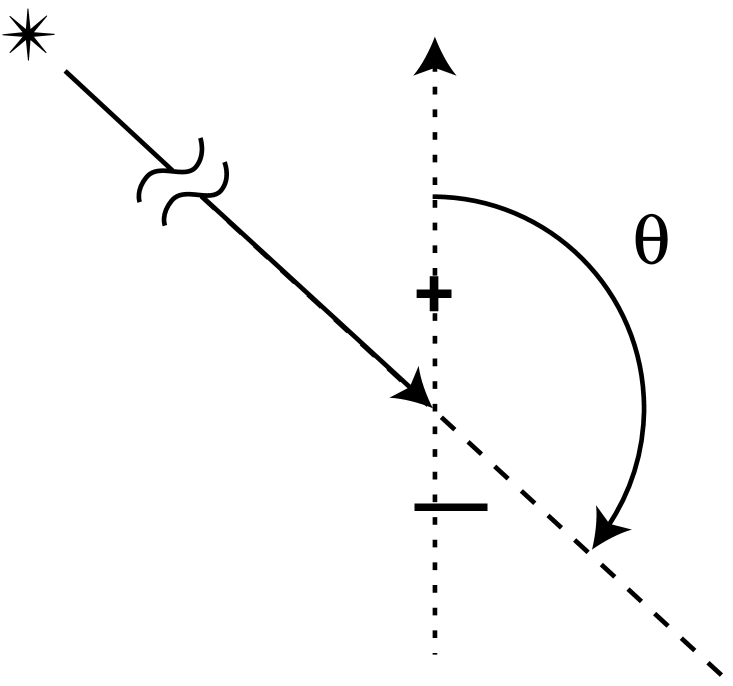
Signals are also characterized by their incident direction relative to the receiver. Since the two detectors have an isotropic antenna pattern, the receiver response to radiation incident from different directions depends only on the angle between the axis defined by the two detectors and the radiation’s propagation direction. Figure 1 shows the geometry we use to describe the interaction of the model receiver with an incident gravitational wave, with the cosine of this angle by $X_{0}$.

Again for the purpose of illustration, consider a model astrophysical burst source population whose members have a well-determined waveform of finite duration. Assume the sources are standard candles and radiate isotropically, with radiation waveform two cycles of a sine wave of known frequency $f_{0}$. Denoting the signal arrival time at the midpoint between the detectors by $T_{0}$ and the signal amplitude as $A_{0}$, the response of the two detectors to the signal is

$$s_{\pm}:=\left\{\begin{array}[]{ll}A_{0}\sin 2\pi f_{0}\left[t-\left(T_{0}\pm RX_{0}\right)\right]&\text{if $0<f_{0}\left[t-\left(T_{0}\pm RX_{0}\right)\right]<2$}\\ 0&\text{otherwise.}\end{array}\right.$$ (82)

where we have dropped the distinction between the signal and the receiver response to the signal and assumed that the detector bandwidth is much greater than the signal bandwidth.

Since $f_{0}$ is known, the receiver response to a signal is fully characterized by $A_{0}$, $T_{0}$ and $X_{0}$. Acting alone, the $\pm$ detector can measure only $A_{0}$ and $T_{\pm}$, where

$$T_{\pm}:=T_{0}\pm RX_{0}.$$ (83)

C Likelihood function

Recall that the receiver’s correlation sequence is

$$\mathchoice{{\hbox{\boldmath$\displaystyle C$}}}{{\hbox{\boldmath$\textstyle C$}}}{{\hbox{\boldmath$\scriptstyle C$}}}{{\hbox{\boldmath$\scriptscriptstyle C$}}}[j-k]=\overline{\mathchoice{{\hbox{\boldmath$\displaystyle n$}}}{{\hbox{\boldmath$\textstyle n$}}}{{\hbox{\boldmath$\scriptstyle n$}}}{{\hbox{\boldmath$\scriptscriptstyle n$}}}[j]\otimes\mathchoice{{\hbox{\boldmath$\displaystyle n$}}}{{\hbox{\boldmath$\textstyle n$}}}{{\hbox{\boldmath$\scriptstyle n$}}}{{\hbox{\boldmath$\scriptscriptstyle n$}}}[k]},$$ (84)

where, for our two detector receiver, each $\mathchoice{{\hbox{\boldmath$\displaystyle C$}}}{{\hbox{\boldmath$\textstyle C$}}}{{\hbox{\boldmath$\scriptstyle C$}}}{{\hbox{\boldmath$\scriptscriptstyle C$}}}[k]$ is a $2\times 2$ matrix. We have assumed that the noise in detector $+$ is uncorrelated with that in detector $-$; consequently, each $\mathchoice{{\hbox{\boldmath$\displaystyle C$}}}{{\hbox{\boldmath$\textstyle C$}}}{{\hbox{\boldmath$\scriptstyle C$}}}{{\hbox{\boldmath$\scriptscriptstyle C$}}}[k]$ is diagonal and the matrix $\mathbb{T}_{N_{T}}(\mathchoice{{\hbox{\boldmath$\displaystyle C$}}}{{\hbox{\boldmath$\textstyle C$}}}{{\hbox{\boldmath$\scriptstyle C$}}}{{\hbox{\boldmath$\scriptscriptstyle C$}}})$ is conveniently re-organized into a $2\times 2$ block diagonal matrix:

$$\left|\left|\mathbb{T}_{N_{T}}(\mathchoice{{\hbox{\boldmath$\displaystyle C$}}}{{\hbox{\boldmath$\textstyle C$}}}{{\hbox{\boldmath$\scriptstyle C$}}}{{\hbox{\boldmath$\scriptscriptstyle C$}}})\right|\right|=\text{diag}\left(\mathchoice{{\hbox{\boldmath$\displaystyle C$}}}{{\hbox{\boldmath$\textstyle C$}}}{{\hbox{\boldmath$\scriptstyle C$}}}{{\hbox{\boldmath$\scriptscriptstyle C$}}}_{{}+{}},\mathchoice{{\hbox{\boldmath$\displaystyle C$}}}{{\hbox{\boldmath$\textstyle C$}}}{{\hbox{\boldmath$\scriptstyle C$}}}{{\hbox{\boldmath$\scriptscriptstyle C$}}}_{{}-{}}\right)=\left(\begin{array}[]{cc}\mathchoice{{\hbox{\boldmath$\displaystyle C$}}}{{\hbox{\boldmath$\textstyle C$}}}{{\hbox{\boldmath$\scriptstyle C$}}}{{\hbox{\boldmath$\scriptscriptstyle C$}}}_{+}&0\\ 0&\mathchoice{{\hbox{\boldmath$\displaystyle C$}}}{{\hbox{\boldmath$\textstyle C$}}}{{\hbox{\boldmath$\scriptstyle C$}}}{{\hbox{\boldmath$\scriptscriptstyle C$}}}_{{}-{}}\end{array}\right),$$ (86)

where $\mathchoice{{\hbox{\boldmath$\displaystyle C$}}}{{\hbox{\boldmath$\textstyle C$}}}{{\hbox{\boldmath$\scriptstyle C$}}}{{\hbox{\boldmath$\scriptscriptstyle C$}}}_{\pm}$ is the correlation matrix for the $\pm$ detector,

$$\left|\left|\mathchoice{{\hbox{\boldmath$\displaystyle C$}}}{{\hbox{\boldmath$\textstyle C$}}}{{\hbox{\boldmath$\scriptstyle C$}}}{{\hbox{\boldmath$\scriptscriptstyle C$}}}_{\pm}\right|\right|_{jk}=\overline{n_{\pm}[j]n_{\pm}[k]}.$$ (87)

Expressed in this way, it is apparent that the likelihood function is separable:

$$\Lambda(\mathchoice{{\hbox{\boldmath$\displaystyle g$}}}{{\hbox{\boldmath$\textstyle g$}}}{{\hbox{\boldmath$\scriptstyle g$}}}{{\hbox{\boldmath$\scriptscriptstyle g$}}}|A,X,T_{0})=\Lambda({g}_{+}|A,T_{{}+{}})\Lambda({g}_{{}-{}}|A,T_{{}-{}})$$ (89)

where

$\displaystyle\ln\Lambda({g}_{{}\pm{}}|A,T_{\pm})$ $\displaystyle=$ $\displaystyle 2<g_{\pm},m(A,T_{\pm})>_{\mathchoice{{\hbox{\boldmath$\displaystyle C$}}}{{\hbox{\boldmath$\textstyle C$}}}{{\hbox{\boldmath$\scriptstyle C$}}}{{\hbox{\boldmath$\scriptscriptstyle C$}}}_{\pm}}-<m(A,T_{\pm},m(A,T_{\pm})>_{\mathchoice{{\hbox{\boldmath$\displaystyle C$}}}{{\hbox{\boldmath$\textstyle C$}}}{{\hbox{\boldmath$\scriptstyle C$}}}{{\hbox{\boldmath$\scriptscriptstyle C$}}}_{\pm}}$ (90)

The $\Lambda({g}_{\pm}|A,T_{\pm})$ are exactly the likelihood functions for the $\pm$ detectors regarded as single, isolated receivers. This separation is always possible when the noise in the detectors is uncorrelated. When the noise in the detectors is correlated the likelihood is still separable once the pseudo-detectors are defined through as described in sec. III E 1.

D Signal detection

In this section we consider, in the context of our model receiver, two different ways one might use a pair of detectors to detect a signal and infer its parameters. One procedure exploits the notion of coincidence: if the two detectors identify separately a signal with sufficiently similar parameters then the receiver is said to have detected a signal. The other procedure exploits the notion of correlation as developed in section III: if the response of an array of detectors is consistent with an incident plane-wave, then the receiver is said to have detected a signal. For each of these two tests we determine the detection efficiency as a function of the false alarm error fraction when the detector noise is Gaussian. We find that the test based on correlation, as embodied in the receiver likelihood function, has a greater detection efficiency than the coincidence test for any choice of false alarm fraction.

1 Maximum Likelihood Inference

The likelihood function $\Lambda(\mathchoice{{\hbox{\boldmath$\displaystyle g$}}}{{\hbox{\boldmath$\textstyle g$}}}{{\hbox{\boldmath$\scriptstyle g$}}}{{\hbox{\boldmath$\scriptscriptstyle g$}}}|\mathchoice{{\hbox{\boldmath$\displaystyle\theta$}}}{{\hbox{\boldmath$\textstyle\theta$}}}{{\hbox{\boldmath$\scriptstyle\theta$}}}{{\hbox{\boldmath$\scriptscriptstyle\theta$}}})$ is the dimensionless ratio of two probabilities: the probability of making the observation $\textstyle g$ if the signal $\textstyle\theta$ is present and the probability of making the observation $\textstyle g$ if no signal is present. It is not a probability itself, nor by itself does it relate directly to a probability on $\textstyle\theta$.

Even though we can’t regard the likelihood as a measure of the probability that a signal characterized by $\textstyle\theta$ is present, we can regard it as a measure of the plausibility of that conclusion: when $\Lambda(\mathchoice{{\hbox{\boldmath$\displaystyle g$}}}{{\hbox{\boldmath$\textstyle g$}}}{{\hbox{\boldmath$\scriptstyle g$}}}{{\hbox{\boldmath$\scriptscriptstyle g$}}}|\mathchoice{{\hbox{\boldmath$\displaystyle\theta$}}}{{\hbox{\boldmath$\textstyle\theta$}}}{{\hbox{\boldmath$\scriptstyle\theta$}}}{{\hbox{\boldmath$\scriptscriptstyle\theta$}}})$ is greater than unity it signals that the particular observation $\textstyle g$ is more likely when the signal characterized by $\textstyle\theta$ is present than when no signal is present. Similarly, if we assume that a signal is present, then the parameter $\textstyle\theta$ that maximizes the likelihood function is the most plausible description of the signal.

Together, these observations motivate a test based on the likelihood function: when the likelihood function maximum $\Lambda(\mathchoice{{\hbox{\boldmath$\displaystyle g$}}}{{\hbox{\boldmath$\textstyle g$}}}{{\hbox{\boldmath$\scriptstyle g$}}}{{\hbox{\boldmath$\scriptscriptstyle g$}}}|\widehat{\mathchoice{{\hbox{\boldmath$\displaystyle\theta$}}}{{\hbox{\boldmath$\textstyle\theta$}}}{{\hbox{\boldmath$\scriptstyle\theta$}}}{{\hbox{\boldmath$\scriptscriptstyle\theta$}}}})$ exceeds a threshold $\Lambda_{0}$, then we conclude that a signal is present and take $\widehat{\mathchoice{{\hbox{\boldmath$\displaystyle\theta$}}}{{\hbox{\boldmath$\textstyle\theta$}}}{{\hbox{\boldmath$\scriptstyle\theta$}}}{{\hbox{\boldmath$\scriptscriptstyle\theta$}}}}$ to be the maximum likelihood estimator, or MLE, of the detected signal.

To be precise, consider an observation $\textstyle g$, whose $N$ samples $\mathchoice{{\hbox{\boldmath$\displaystyle g$}}}{{\hbox{\boldmath$\textstyle g$}}}{{\hbox{\boldmath$\scriptstyle g$}}}{{\hbox{\boldmath$\scriptscriptstyle g$}}}[k]$ are taken at time $t_{k}$. Denote by $\mathchoice{{\hbox{\boldmath$\displaystyle s$}}}{{\hbox{\boldmath$\textstyle s$}}}{{\hbox{\boldmath$\scriptstyle s$}}}{{\hbox{\boldmath$\scriptscriptstyle s$}}}(\mathchoice{{\hbox{\boldmath$\displaystyle\theta$}}}{{\hbox{\boldmath$\textstyle\theta$}}}{{\hbox{\boldmath$\scriptstyle\theta$}}}{{\hbox{\boldmath$\scriptscriptstyle\theta$}}})[j]$ the sampled receiver response to a signal characterized by $\textstyle\theta$. Assume that the observation duration is much longer than the longest signal response (so that we need not consider signals that begin before or end after the observation period). Denote by $\mathchoice{{\hbox{\boldmath$\displaystyle\theta$}}}{{\hbox{\boldmath$\textstyle\theta$}}}{{\hbox{\boldmath$\scriptstyle\theta$}}}{{\hbox{\boldmath$\scriptscriptstyle\theta$}}}_{k}$ the parameter space of signals whose leading wavefront is incident on the receiver at time $t_{k}$: in our example, these are just $A$ and $X$. Finally, fix a threshold $\rho^{2}_{0}$. The following procedure produces a list of detected signals and point estimates of the parameters describing each:

  1. 1.

    Evaluate the log-likelihood function $\ln\Lambda(\mathchoice{{\hbox{\boldmath$\displaystyle g$}}}{{\hbox{\boldmath$\textstyle g$}}}{{\hbox{\boldmath$\scriptstyle g$}}}{{\hbox{\boldmath$\scriptscriptstyle g$}}}|\mathchoice{{\hbox{\boldmath$\displaystyle\theta$}}}{{\hbox{\boldmath$\textstyle\theta$}}}{{\hbox{\boldmath$\scriptstyle\theta$}}}{{\hbox{\boldmath$\scriptscriptstyle\theta$}}}_{k})$ for signals incident on the receiver at the sample times $t_{k}$.

  2. 2.

    At each sample time $t_{k}$, find the signal characterization $\widehat{\mathchoice{{\hbox{\boldmath$\displaystyle\theta$}}}{{\hbox{\boldmath$\textstyle\theta$}}}{{\hbox{\boldmath$\scriptstyle\theta$}}}{{\hbox{\boldmath$\scriptscriptstyle\theta$}}}}_{k}$ that maximizes $\ln\Lambda(\mathchoice{{\hbox{\boldmath$\displaystyle g$}}}{{\hbox{\boldmath$\textstyle g$}}}{{\hbox{\boldmath$\scriptstyle g$}}}{{\hbox{\boldmath$\scriptscriptstyle g$}}}|\mathchoice{{\hbox{\boldmath$\displaystyle\theta$}}}{{\hbox{\boldmath$\textstyle\theta$}}}{{\hbox{\boldmath$\scriptstyle\theta$}}}{{\hbox{\boldmath$\scriptscriptstyle\theta$}}}_{k})$. Associate with each $t_{k}$ and $\widehat{\mathchoice{{\hbox{\boldmath$\displaystyle\theta$}}}{{\hbox{\boldmath$\textstyle\theta$}}}{{\hbox{\boldmath$\scriptstyle\theta$}}}{{\hbox{\boldmath$\scriptscriptstyle\theta$}}}}_{k}$ a S/N $\widehat{\rho}_{k}$, given by

    $$\widehat{\rho}^{2}_{k}=\ln\Lambda(\mathchoice{{\hbox{\boldmath$\displaystyle g$}}}{{\hbox{\boldmath$\textstyle g$}}}{{\hbox{\boldmath$\scriptstyle g$}}}{{\hbox{\boldmath$\scriptscriptstyle g$}}}|\widehat{\mathchoice{{\hbox{\boldmath$\displaystyle\theta$}}}{{\hbox{\boldmath$\textstyle\theta$}}}{{\hbox{\boldmath$\scriptstyle\theta$}}}{{\hbox{\boldmath$\scriptscriptstyle\theta$}}}}_{k}).$$ (91)
  3. 3.

    Order the triplets $\{\widehat{\rho}_{k},\widehat{\mathchoice{{\hbox{\boldmath$\displaystyle\theta$}}}{{\hbox{\boldmath$\textstyle\theta$}}}{{\hbox{\boldmath$\scriptstyle\theta$}}}{{\hbox{\boldmath$\scriptscriptstyle\theta$}}}}_{k},t_{k}\}$ with respect to $t_{k}$. Select the subset of triplets where i) $\rho_{k}$ is greater than the threshold $\rho_{0}$ and ii) a local maxima; i.e., find the $\{\widehat{\rho}_{k^{\prime}},\widehat{\mathchoice{{\hbox{\boldmath$\displaystyle\theta$}}}{{\hbox{\boldmath$\textstyle\theta$}}}{{\hbox{\boldmath$\scriptstyle\theta$}}}{{\hbox{\boldmath$\scriptscriptstyle\theta$}}}}_{k^{\prime}}\}$ for which

    $\displaystyle\rho_{0}$ $\displaystyle<$ $\displaystyle\widehat{\rho}_{\pm,k^{\prime}}$ (93)
    $\displaystyle\widehat{\rho}_{\pm,k^{\prime}-1}$ $\displaystyle\leq$ $\displaystyle\widehat{\rho}_{\pm,k^{\prime}}$ (94)
    $\displaystyle\widehat{\rho}_{\pm,k^{\prime}+1}$ $\displaystyle\leq$ $\displaystyle\widehat{\rho}_{\pm,k^{\prime}}.$ (95)
  4. 4.

    Beginning with the largest $\widehat{\rho}_{k}$ in this subset find all other triplets $\{\widehat{\rho}_{k^{\prime}},\widehat{\mathchoice{{\hbox{\boldmath$\displaystyle\theta$}}}{{\hbox{\boldmath$\textstyle\theta$}}}{{\hbox{\boldmath$\scriptstyle\theta$}}}{{\hbox{\boldmath$\scriptscriptstyle\theta$}}}}_{k^{\prime}},t_{k^{\prime}}\}$ for which $|t_{k}-t_{k^{\prime}}|$ is less than the signal duration. Discard these tripletts. Repeat with the next largest remaining $\widehat{\rho}_{k}$ until the list is exhausted. What remains is the list of detected signals, with S/N $\widehat{\rho}_{k}$, signal start time $t_{k}$, and characterized by (the point estimate) $\widehat{\mathchoice{{\hbox{\boldmath$\displaystyle\theta$}}}{{\hbox{\boldmath$\textstyle\theta$}}}{{\hbox{\boldmath$\scriptstyle\theta$}}}{{\hbox{\boldmath$\scriptscriptstyle\theta$}}}}_{k}$.

Three steps in the maximum likelihood test procedure deserve additional discussion: the focus only on bursts starting at the discrete sample times $t_{k}$ (step 2), the formation of the intermediate list of consisting of local maxima of the maximum of the likelihood function (step 3) and the pruning of this list to form the final list of detected signals (step 4).

Step 2 focuses attention on signals arriving at the discrete sample times. Real signals, however, are not so constrained. Nevertheless, if the observation is properly sampled (i.e., sampled without aliasing), then all of the power in the receiver response is at frequencies much less than the Nyquist frequency $f_{N}$, which is half the sample rate. In that case $\left<\mathchoice{{\hbox{\boldmath$\displaystyle m$}}}{{\hbox{\boldmath$\textstyle m$}}}{{\hbox{\boldmath$\scriptstyle m$}}}{{\hbox{\boldmath$\scriptscriptstyle m$}}}(\mathchoice{{\hbox{\boldmath$\displaystyle\theta$}}}{{\hbox{\boldmath$\textstyle\theta$}}}{{\hbox{\boldmath$\scriptstyle\theta$}}}{{\hbox{\boldmath$\scriptscriptstyle\theta$}}},t_{0}),\mathchoice{{\hbox{\boldmath$\displaystyle m$}}}{{\hbox{\boldmath$\textstyle m$}}}{{\hbox{\boldmath$\scriptstyle m$}}}{{\hbox{\boldmath$\scriptscriptstyle m$}}}(\mathchoice{{\hbox{\boldmath$\displaystyle\theta$}}}{{\hbox{\boldmath$\textstyle\theta$}}}{{\hbox{\boldmath$\scriptstyle\theta$}}}{{\hbox{\boldmath$\scriptscriptstyle\theta$}}},t_{0}+\tau)\right>_{\mathchoice{{\hbox{\boldmath$\displaystyle C$}}}{{\hbox{\boldmath$\textstyle C$}}}{{\hbox{\boldmath$\scriptstyle C$}}}{{\hbox{\boldmath$\scriptscriptstyle C$}}}}$, where $\mathchoice{{\hbox{\boldmath$\displaystyle m$}}}{{\hbox{\boldmath$\textstyle m$}}}{{\hbox{\boldmath$\scriptstyle m$}}}{{\hbox{\boldmath$\scriptscriptstyle m$}}}(\mathchoice{{\hbox{\boldmath$\displaystyle\theta$}}}{{\hbox{\boldmath$\textstyle\theta$}}}{{\hbox{\boldmath$\scriptstyle\theta$}}}{{\hbox{\boldmath$\scriptscriptstyle\theta$}}},t)$ denotes the receiver response to a signal whose initial wavefront arrives at the network at time $t$, cannot vary significantly for $|\tau|$ less than several times $1/f_{N}$; correspondingly, the likelihood will remain peaked about the $t_{k}$ nearest to the actual signal arrival time and the corresponding signal to noise will differ only slightly from its maximum value.The errors incurred here can be reduced still further by appropriate interpolation.

In step 3, we select only the local maxima of the likelihood function as candidate signal events. This reflects the observation that, in the absence of noise, the likelihood function is maximized when $\textstyle\theta$ is equal to the true signal characterization $\mathchoice{{\hbox{\boldmath$\displaystyle\theta$}}}{{\hbox{\boldmath$\textstyle\theta$}}}{{\hbox{\boldmath$\scriptstyle\theta$}}}{{\hbox{\boldmath$\scriptscriptstyle\theta$}}}_{t}$.

Even in the absence of noise, however, not all local maxima can be identified as distinct signals. While the likelihood function is maximized when $\textstyle\theta$ is equal to the true signal characterization $\mathchoice{{\hbox{\boldmath$\displaystyle\theta$}}}{{\hbox{\boldmath$\textstyle\theta$}}}{{\hbox{\boldmath$\scriptstyle\theta$}}}{{\hbox{\boldmath$\scriptscriptstyle\theta$}}}_{t}$, as $\textstyle\theta$ differs from $\mathchoice{{\hbox{\boldmath$\displaystyle\theta$}}}{{\hbox{\boldmath$\textstyle\theta$}}}{{\hbox{\boldmath$\scriptstyle\theta$}}}{{\hbox{\boldmath$\scriptscriptstyle\theta$}}}_{t}$ the likelihood decreases, but not necessarily monotonically. Even for our simple signal model there are three local maxima associated with the likelihood function. The situation is further complicated when, as is the actual case, receiver noise distorts the “noise-free” likelihood, randomly increasing it for some $\mathchoice{{\hbox{\boldmath$\displaystyle\theta$}}}{{\hbox{\boldmath$\textstyle\theta$}}}{{\hbox{\boldmath$\scriptstyle\theta$}}}{{\hbox{\boldmath$\scriptscriptstyle\theta$}}}_{k}$ and decreasing it for others.

To help distinguish between the global maximum of the likelihood function and its sidelobes, we make use of our implicit assumption that real signals are sufficiently rare that the receiver response to one real signal does not have a significant probability of overlapping with its response to a second real signal. Any two local maxima separated in time by less than the signal duration are then associated with a single source. In step 4 we prune the list of candidate signals (i.e., the local maxima identified in step 3) by identifying clusters of local maxima and replacing each with its single, strongest member.This intrinsically non-linear step introduces into the analysis a notion of detector “dead time:” i.e., the analysis is unable to identify more than a single signal in any given interval of duration less than the signal duration. The result is a list of events, all above threshold, in which no two events can have resulted from the same gravitational-wave signal.

Finally, we justify the use of $\widehat{\mathchoice{{\hbox{\boldmath$\displaystyle\theta$}}}{{\hbox{\boldmath$\textstyle\theta$}}}{{\hbox{\boldmath$\scriptstyle\theta$}}}{{\hbox{\boldmath$\scriptscriptstyle\theta$}}}}$ as the point estimate of the signal parameters characterizing the detected signal. Suppose that a signal characterized by fixed $\mathchoice{{\hbox{\boldmath$\displaystyle\theta$}}}{{\hbox{\boldmath$\textstyle\theta$}}}{{\hbox{\boldmath$\scriptstyle\theta$}}}{{\hbox{\boldmath$\scriptscriptstyle\theta$}}}_{t}$ is incident on an ensemble of identical receivers. The corresponding ensemble of $\widehat{\mathchoice{{\hbox{\boldmath$\displaystyle\theta$}}}{{\hbox{\boldmath$\textstyle\theta$}}}{{\hbox{\boldmath$\scriptstyle\theta$}}}{{\hbox{\boldmath$\scriptscriptstyle\theta$}}}}$ has as its mode $\mathchoice{{\hbox{\boldmath$\displaystyle\theta$}}}{{\hbox{\boldmath$\textstyle\theta$}}}{{\hbox{\boldmath$\scriptstyle\theta$}}}{{\hbox{\boldmath$\scriptscriptstyle\theta$}}}_{t}$; consequently, a natural estimator for $\mathchoice{{\hbox{\boldmath$\displaystyle\theta$}}}{{\hbox{\boldmath$\textstyle\theta$}}}{{\hbox{\boldmath$\scriptstyle\theta$}}}{{\hbox{\boldmath$\scriptscriptstyle\theta$}}}_{t}$ is the $\widehat{\mathchoice{{\hbox{\boldmath$\displaystyle\theta$}}}{{\hbox{\boldmath$\textstyle\theta$}}}{{\hbox{\boldmath$\scriptstyle\theta$}}}{{\hbox{\boldmath$\scriptscriptstyle\theta$}}}}$ arising from a particular observation. In the maximum likelihood rule, when we conclude that a signal is present we take $\widehat{\mathchoice{{\hbox{\boldmath$\displaystyle\theta$}}}{{\hbox{\boldmath$\textstyle\theta$}}}{{\hbox{\boldmath$\scriptstyle\theta$}}}{{\hbox{\boldmath$\scriptscriptstyle\theta$}}}}$ as our point-estimate of the signal parameters.

2 Coincidence inference

Much discussed in the context of gravitational-wave data analysis is an apparently simpler analysis, referred to generally as “coincidence.” This test has received its most precise definition in [10, 11] for the particular case of binary inspiral observations.

In general, coincidence tests involve a complete analysis at each individual detector, considered in isolation from all other detectors in the receiver. The result of these individual analyses is a set of “candidate-event lists”, one for each detector, which consist of “detections” at each detector together with estimators for the signal start time and other signal parameters that can be determined from observations in a single detector. Real gravitational-wave events should excite the several different detectors in a self-consistent manner: in particular, the signal start times should be consistent with the light travel time between the detectors and other signal parameters should be consistent with a unique source.

The consistency requirement is difficult to pin-down. For example, in the case of our own model detector and source, consistency would appear to require that the signal arrival times are consistent with the signal propagation time between the detectors and that the measured signal amplitudes be equal. Owing to detector noise, however, the estimated signal amplitudes will only approximate the actual amplitudes, and similarly for the signal start times and other parameters. For signal amplitudes, then, a window of some breadth must be defined and signal candidates whose amplitudes fall within the window are assumed to arise from a real signal. The choice of window, its implementation and the procedure for combining separate estimates of common parameters all affect the false alarm and false dismissal fractions that characterize the test.

The problem is more complicated in the case of an estimated source location. Consider a real signal, incident on the detectors from a direction nearly perpendicular to the axis between them. Let the measured start time $T_{\pm}$ on the $\pm$ detector be

$$T_{\pm}=T_{0,\pm}+\epsilon_{\pm},$$ (96)

where $T_{0,\pm}$ is the actual moment when the signal is incident on the $\pm$ detector and $\epsilon_{\pm}$ is the error in the estimated start time owing to detector noise. The difference in the measured signal start times is

$\displaystyle T_{+}-T_{-}$ $\displaystyle=$ $\displaystyle T_{0,+}-T_{0,-}+\epsilon_{+}-\epsilon_{-}$ (97)
$\displaystyle=$ $\displaystyle 2RX_{0}+\Delta{\epsilon},$ (98)

where $X_{0}$ is the direction cosine describing the radiation’s propagation direction and $\Delta{\epsilon}$ is the difference between the errors in the measured start times. When a real signal is incident along, or nearly along, the axis ($|X_{0}|\simeq 1$), then small errors $|\Delta\epsilon|\ll 2R$ can lead to $|\widehat{X}_{0}|>1$, which we would regard as unphysical and not representative of a real signal. On the other hand, when $|X_{0}|$ is much less than unity, the same errors will leave us with $|\widehat{X}_{0}|$ still much less than unity, in which case we accept the coincidence as representing a real signal. To minimize this false rejection of real signals we can adopt a window broader than the light travel time between the detectors for comparing signal arrival times (taking the estimated arrival direction to be along the axis if the difference of arrival times would suggest $|X|$ greater than unity); however, in doing so we also increase the false alarm rate, reducing the discriminating power of the test.

The sign of the error also plays an important role: when $\Delta{\epsilon}$ has the same sign as $X_{0}$ we are more likely to reject a real signal than when they have opposite signs. The fraction of signals rejected can thus depend in a complicated way on the interaction between the underlying signal parameters, the windows, and the allowable range of the parameters that characterize the signal.

In the spirit of [10, 11] we define a coincidence inference procedure for our model receiver:

  1. 1.

    For each detector considered in isolation, determine the two sets of candidate signals associated with detector $+$ and $-$:

    1. (a)

      Evaluate the log-likelihood function $\ln\Lambda({g}_{\pm}|\mathchoice{{\hbox{\boldmath$\displaystyle\theta$}}}{{\hbox{\boldmath$\textstyle\theta$}}}{{\hbox{\boldmath$\scriptstyle\theta$}}}{{\hbox{\boldmath$\scriptscriptstyle\theta$}}}_{\pm,k})$ for signals incident on detector $\pm$ at the sample times $t_{\pm,k}$.

    2. (b)

      At each sample time $t_{\pm,k}$, find the signal characterization $\widehat{\mathchoice{{\hbox{\boldmath$\displaystyle\theta$}}}{{\hbox{\boldmath$\textstyle\theta$}}}{{\hbox{\boldmath$\scriptstyle\theta$}}}{{\hbox{\boldmath$\scriptscriptstyle\theta$}}}}_{\pm,k}$ that maximizes $\ln\Lambda({g}_{\pm}|\mathchoice{{\hbox{\boldmath$\displaystyle\theta$}}}{{\hbox{\boldmath$\textstyle\theta$}}}{{\hbox{\boldmath$\scriptstyle\theta$}}}{{\hbox{\boldmath$\scriptscriptstyle\theta$}}}_{\pm,k})$. Associate with each $t_{\pm,k}$ and $\widehat{\mathchoice{{\hbox{\boldmath$\displaystyle\theta$}}}{{\hbox{\boldmath$\textstyle\theta$}}}{{\hbox{\boldmath$\scriptstyle\theta$}}}{{\hbox{\boldmath$\scriptscriptstyle\theta$}}}}_{\pm,k}$ a S/N $\widehat{\rho}_{\pm,k}$, given by

      $$\widehat{\rho}^{2}_{\pm,k}=\ln\Lambda({g}_{\pm}|\widehat{\mathchoice{{\hbox{\boldmath$\displaystyle\theta$}}}{{\hbox{\boldmath$\textstyle\theta$}}}{{\hbox{\boldmath$\scriptstyle\theta$}}}{{\hbox{\boldmath$\scriptscriptstyle\theta$}}}}_{\pm,k}).$$ (99)

      The result is a set of associated signal-to-noise, parameterizations and signal start times $\{\widehat{\rho}_{\pm,k},\widehat{\mathchoice{{\hbox{\boldmath$\displaystyle\theta$}}}{{\hbox{\boldmath$\textstyle\theta$}}}{{\hbox{\boldmath$\scriptstyle\theta$}}}{{\hbox{\boldmath$\scriptscriptstyle\theta$}}}}_{\pm,k},{t}_{\pm,k}\}$.

    3. (c)

      For the list associated with each detector, select the subset $\{\widehat{\rho}_{\pm,k^{\prime}},\widehat{\mathchoice{{\hbox{\boldmath$\displaystyle\theta$}}}{{\hbox{\boldmath$\textstyle\theta$}}}{{\hbox{\boldmath$\scriptstyle\theta$}}}{{\hbox{\boldmath$\scriptscriptstyle\theta$}}}}_{\pm,k^{\prime}},t_{\pm,k^{\prime}}\}$ for which

      $\displaystyle\widehat{\rho}_{\pm,0}$ $\displaystyle<$ $\displaystyle\rho_{\pm,k^{\prime}}$ (101)
      $\displaystyle\widehat{\rho}_{\pm,k^{\prime}-1}$ $\displaystyle\leq$ $\displaystyle\rho_{\pm,k^{\prime}}$ (102)
      $\displaystyle\widehat{\rho}_{\pm,k^{\prime}+1}$ $\displaystyle\leq$ $\displaystyle\rho_{\pm,k^{\prime}}$ (103)

      where $\widehat{\rho}_{\pm,0}$ is the signal detection threshold in detector $\pm$.

    4. (d)

      Beginning with the largest $\widehat{\rho}_{\pm,k}$ in the list of local maxima associated with detector $\pm$, find all other $\widehat{\rho}_{\pm,k^{\prime}}$ for which $|t_{k}-t_{k^{\prime}}|$ is less than the signal duration. Discard these. Repeat with the next largest remaining $\widehat{\rho}_{\pm,k}$ until the list is exhausted. What remains is the list of candidate signals, with S/N $\widehat{\rho}_{\pm,0}$, signal start time $t_{\pm,k}$, and characterized by (the point estimate) $\widehat{\mathchoice{{\hbox{\boldmath$\displaystyle\theta$}}}{{\hbox{\boldmath$\textstyle\theta$}}}{{\hbox{\boldmath$\scriptstyle\theta$}}}{{\hbox{\boldmath$\scriptscriptstyle\theta$}}}}_{\pm,k}$.

  2. 2.

    Choose the candidate signal list associated with detector $+$. Beginning with the candidate signal of largest S/N $\widehat{\rho}_{+,k}$ in that list, process that list in order of decreasing $\widehat{\rho}_{+,k}$ to create a new, coincident detection event list:

    1. (a)

      Let the current candidate event from the list associated with detector $+$ be numbered $k_{+}$.

    2. (b)

      Identify, from the candidate event list associated with detector $-$, all candidates whose start times $t_{j_{-}}$ in detector $-$ are consistent with the candidate signal arrival time $t_{k_{+}}$ in detector $+$: i.e.,

      $$|t_{k_{+}}-t_{j_{-}}|<2R.$$ (104)

      Impose other consistency requirements, associated with $\widehat{\mathchoice{{\hbox{\boldmath$\displaystyle\theta$}}}{{\hbox{\boldmath$\textstyle\theta$}}}{{\hbox{\boldmath$\scriptstyle\theta$}}}{{\hbox{\boldmath$\scriptscriptstyle\theta$}}}}_{+,k_{+}}$ and $\widehat{\mathchoice{{\hbox{\boldmath$\displaystyle\theta$}}}{{\hbox{\boldmath$\textstyle\theta$}}}{{\hbox{\boldmath$\scriptstyle\theta$}}}{{\hbox{\boldmath$\scriptscriptstyle\theta$}}}}_{-,j_{-}}$, as are deemed appropriate. (In our model receiver/source example we do not impose any other consistency requirements.)

    3. (c)

      The result is a list of candidate coincident events in detector $-$ associated with the event $k_{+}$ in detector $+$. The list may contain zero, one or more than one event:

      1. i.

        If it contains no events, delete event $k_{+}$ from the list of candidate events associated with detector $+$.

      2. ii.

        If it contains exactly one event (say, $\{\widehat{\rho}_{-,j_{-}}$, $\widehat{\mathchoice{{\hbox{\boldmath$\displaystyle\theta$}}}{{\hbox{\boldmath$\textstyle\theta$}}}{{\hbox{\boldmath$\scriptstyle\theta$}}}{{\hbox{\boldmath$\scriptscriptstyle\theta$}}}}_{-,j_{-}}$, $t_{-,j_{-}}\}$), pair it with the event $\{\widehat{\rho}_{+,k_{+}}$, $\widehat{\mathchoice{{\hbox{\boldmath$\displaystyle\theta$}}}{{\hbox{\boldmath$\textstyle\theta$}}}{{\hbox{\boldmath$\scriptstyle\theta$}}}{{\hbox{\boldmath$\scriptscriptstyle\theta$}}}}_{+,k_{+}}$, $t_{+,k_{+}}\}$ from the list associated with detector $+$ and add the pair to the coincident detection event list. Delete all events from the candidate list associated with detector $+$ whose arrival times are so close that they would overlap with event $k_{+}$; similarly, delete all events from the candidate list associated with detector $-$ whose arrival times are so close that they would overlap with event $j_{-}$. Delete events $k_{+}$ and $j_{-}$ from their respective candidate lists.

      3. iii.

        If it contains more than one event, choose the single event $j_{-}$ with greatest strength $\widehat{\rho}_{-,j}$, pair it with event $k_{+}$ from the candidate list associated with detector $+$, and add the pair to the coincident detection event list. Delete all events from the candidate list associated with detector $+$ whose arrival times $t_{+,k}$ are so close that they would overlap with event $k_{+}$; similarly, delete all events from the list associated with detector $-$ whose arrival times $t_{-,j}$ are so close that they would overlap with event $j_{-}$. Delete events $k_{+}$ and $j_{-}$ from the lists associated with the respective detectors.

The result of applying this procedure to the output of the $\pm$ detectors is a set of paired events, one from each detector. Each member of the set involves a pair of signal amplitudes (in this case, equivalent to S/N) and the best estimate of the signal arrival time at each detector. The signal arrival times are, by construction, consistent with the incidence of a plane wave on the detector pair.

It remains to combine the signal arrival times and amplitudes in each pair to determine a single estimate of the signal amplitude, the signal arrival time at the mid-point between the detector, and the radiation propagation direction. In our model problem, the natural estimators for the latter two quantities are

$\displaystyle\widehat{T}_{j}$ $\displaystyle=$ $\displaystyle\left(t_{+,j}+t_{-,j}\right)/2$ (106)
$\displaystyle\widehat{X}_{j}$ $\displaystyle=$ $\displaystyle\left(t_{+,j}-t_{-,j}\right)/2R.$ (107)

The geometry of our model problem suggests no particular procedure for combining the separate signal amplitude estimates into an overall estimate for the network. One procedure that has been recommended [10, 11] is to form the final estimate as the root mean square of the point estimates:

$$\widehat{A}^{2}_{j}={1\over 2}\left(\widehat{A}_{+,j}^{2}+\widehat{A}_{-,j}^{2}\right),$$ (109)

where

$$\widehat{A}_{\pm}:={\rho^{2}_{\pm}\over\left<s_{\pm},s_{\pm}\right>_{C_{\pm}}}$$ (110)

This prescription will consistently overestimate the amplitude of the signal. For any given observation of a signal with amplitude $A_{0}$, the estimate in the detector $\pm$ is equal to $A_{0}$ plus a random variable:

$$\widehat{A}_{\pm}=A_{0}+n_{\pm}.$$ (111)

If the detector noise is Gaussian then $n_{\pm}$ is Gaussian. The mean square of the point estimates is thus

$$\widehat{A}^{2}=A_{0}^{2}+A_{0}\left(n_{+}+n_{-}\right)+{1\over 2}\left(n_{+}^{2}+n_{-}^{2}\right).$$ (112)

The mean of $\widehat{A}^{2}$, or of $\widehat{A}$, will thus be greater than $A_{0}$. A similar problem will plague any attempt to form network estimates of parameters from parameters that are overdetermined by the network (for example, network-wide estimates of $T$ or $X$ from three or more detectors).

An unbiased estimate for $A_{0}$ is the straightforward average of the parameter values, which we adopt here:

$$\widehat{A}_{j}:={1\over 2}\left(\widehat{A}_{+,j}+\widehat{A}_{-,j}\right),$$ (114)

where

$$\widehat{A}_{\pm,k}:={\left<g_{\pm},s_{\pm,\widehat{\mathchoice{{\hbox{\boldmath$\displaystyle\theta$}}}{{\hbox{\boldmath$\textstyle\theta$}}}{{\hbox{\boldmath$\scriptstyle\theta$}}}{{\hbox{\boldmath$\scriptscriptstyle\theta$}}}}_{\pm,k}}\right>\over\sqrt{\left<s_{\pm,\widehat{\mathchoice{{\hbox{\boldmath$\displaystyle\theta$}}}{{\hbox{\boldmath$\textstyle\theta$}}}{{\hbox{\boldmath$\scriptstyle\theta$}}}{{\hbox{\boldmath$\scriptscriptstyle\theta$}}}}_{\pm,k}},s_{\pm,\widehat{\mathchoice{{\hbox{\boldmath$\displaystyle\theta$}}}{{\hbox{\boldmath$\textstyle\theta$}}}{{\hbox{\boldmath$\scriptstyle\theta$}}}{{\hbox{\boldmath$\scriptscriptstyle\theta$}}}}_{\pm,k}}\right>}}.$$ (115)

Several aspects of this procedure for detecting a signal coincident in two detectors and estimating the parameters characteristic of the source deserve special attention:

a Candidate signals.

Each event in a pair identified as a coincident detection stands on its own as a detection in its detector at the given threshold.

b Estimator bias.

When the noise distribution is Gaussian, the error in the estimator of the signal arrival time at a particular detector is also Gaussian. Consequently it might be thought that the error in the estimators $\widehat{T}_{j}$ and $\widehat{X}_{j}$ are also normal, since they arise from the combination of normal errors in two detectors whose noise is normal, and that the estimators $\widehat{T}_{j}$ and $\widehat{X}_{j}$ are unbiased. (This is the claim is made in [10, 11].) As discussed above, however, the errors in the $t_{\pm,j}$ are correlated by the procedure we used to create the coincident detection list: for radiation whose propagation direction is nearly aligned with the axis between the detectors, insisting that $|t_{+,j}-t_{-,j}|$ be less than $2R$ causes us to favor those signals for which the errors in $t_{+,j}$ and $t_{-,j}$ are positively correlated. The estimator $X_{j}$ in equation 107 is thus biased to underestimate the magnitude of the propagation direction cosine; additionally, signals whose propagation direction cosine is large (i.e., signals propagated along or nearly along the axis) have larger false dismissal fractions than signals propagating normal to the axis.

c Signal strength.

In the maximum likelihood test described above, signal strength is described by a single quantity: the S/N, which is equal to the log maximum likelihood. This measure of signal strength has the desired property that, as the detection threshold is increased, weaker signals are no longer considered to be detected before stronger signals. In the coincidence test, there are two different “signal-to-noise” ratios — one for each detector — and neither, by itself, is sufficient to determine that a signal is present. It has been suggested [10, 11] that the “natural” signal strength for coincidence tests is the sum of the amplitude-squared S/N for the different detectors: in this case

$$\widehat{\rho}_{j}^{2}=\widehat{\rho}_{+,j}^{2}+\widehat{\rho}_{-,j}^{2}.$$ (116)

This definition has the undesirable property that “stronger” signals (i.e., those with larger $\widehat{\rho}$) are not necessarily more likely to be detected than weaker ones. In particular, as the detection thresholds are raised at the two detectors, signals disappear from the coincident detection list when the weakest member of the pair $\{\widehat{\rho}_{+},\widehat{\rho}_{-}\}$ falls below the threshold in the $\pm$ detector, which is not when $\rho^{2}$ falls below threshold. If we want signal strength to have the property that, as the detection threshold is increased, weaker signals disappear from the detection list before stronger ones then the appropriate measure of signal strength is the minimum of $\widehat{\rho}_{+}$ and $\widehat{\rho}_{-}$:§§§When the several detectors in the network are not identical, or do not have coincident or isotropic antenna patterns, then the criteria that weaker signals are always less likely to be detected than stronger ones becomes more difficult to determine.

$$\widehat{\rho}\equiv\min(\widehat{\rho}_{+},\widehat{\rho}_{-}).$$ (117)

The detection rule described in this section is not the only such rule in the spirit of coincidence that can be defined. Many variations are possible, corresponding to the many ad hoc decisions that must be made, especially in identifying candidate events lists for the separate detectors and identifying “consistent” coincidences. The choices made here are among the simplest that lead to a well-defined procedure for identifying coincident events.

3 Gaussian Noise

To assess the relative performance of the maximum likelihood and coincidence inference rules we use Monte Carlo simulations to calculate the false alarm and false dismissal fractions $\alpha$ and $\beta$ as well as the distributions of the estimators $\widehat{T}_{0}$, $\widehat{X}$ and $\widehat{A}_{0}$ for a typical signal.

An inference rule’s false alarm frequency $\dot{N}_{\alpha}$ is the limiting frequency of “signal detection” when, in fact, no signal is actually present. To determine $\dot{N}_{\alpha}$ as a function of the threshold $\rho_{0}^{2}$ we use a statistical model of the receiver noise to generate many pseudo-random instances of $\textstyle g$ representative of receiver noise alone. The false alarm frequency is then the average number of “detections” per unit time. A convenient, dimensionless representation of the false alarm frequency is the average number of false signals detected per sample $\mathchoice{{\hbox{\boldmath$\displaystyle g$}}}{{\hbox{\boldmath$\textstyle g$}}}{{\hbox{\boldmath$\scriptstyle g$}}}{{\hbox{\boldmath$\scriptscriptstyle g$}}}[k]$:

$$\alpha\equiv\dot{N}_{\alpha}/f_{s},$$ (118)

where $f_{s}$ is the sample rate. We refer to $\alpha$ as the false alarm fraction; by our procedure $\alpha$ is strictly less than or equal to unity and can be regarded as the probability of a false detection on a per-sample basis.

The false dismissal frequency $\beta$ of an inference rule is the limiting frequency with which the rule reports that no signal is present when, in fact, a signal is present; thus, $\beta$ is a function of the signal (or the signal population). Another way to think about $\beta$ is as the detection efficiency: $1-\beta$ is the fraction of actual signals that the detection procedure will identify. To find $\beta$ we generate many pseudo-random instances of receiver noise and add to them a specific signal. The result is many instances of $\textstyle g$ corresponding to observations of that source. The inference rule will conclude that no signal is present in some fraction of these synthetic observations: that fraction is the false dismissal fraction.

In the case of the maximum likelihood test, $\alpha$ and $\beta$ are controlled by adjusting the threshold $\rho_{0}$: as $\rho_{0}$ is increased, $\alpha$ is decreased. In the case of the coincidence test described in section IV D 2, $\alpha$ and $\beta$ are controlled by adjusting the two thresholds $\rho_{\pm,0}$. Since, in our example, the two detectors are identical, we set these equal to the same $\rho_{0}$. The false dismissal frequency depends on the distribution of signals in the signal population; for simplicity, we assume that all signals in the population have the same unknown amplitude $A_{0}$ and sky location $X_{0}$, which are given in the first column of table III.

(More realistically the amplitude $A$ depends inversely on the distance to the source, its orientation with respect to the detector, and other parameters. Corresponding to the source distribution in space and the other parameters is a distribution for $A$. Requiring that $\alpha$ not exceed a certain value sets a threshold $\Lambda_{0}$, regardless of this distribution. The false dismissal frequency $\beta$, on the other hand, depends on this distribution in a straightforward way.)
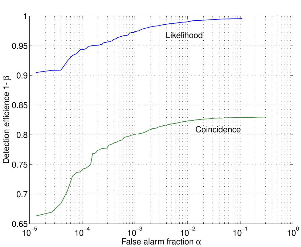
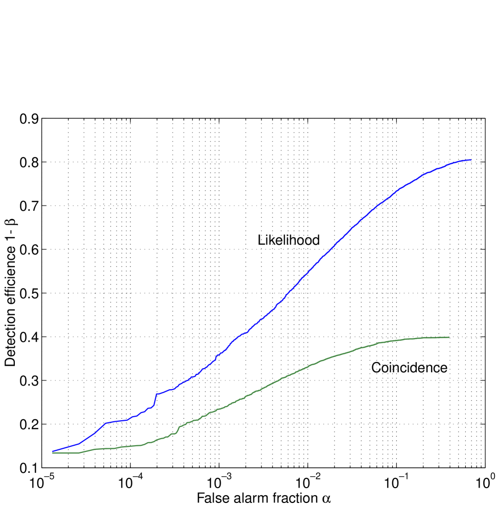
Figure 2 shows $1-\beta$ as a function of $\alpha$ for the maximum likelihood and coincidence detection procedures when used to detect signals of this character in our model receiver. In these Monte Carlo simulations we count as a false dismissal all signal identifications (whether by the coincidence or maximum likelihood test) where the identified start time $\widehat{T}$ differs from the actual start time by more than the signal duration, or where the identified sky position $\widehat{X}$ differs from actual sky position by more than the signal duration divided by the detector separation. This condition is necessary if “correct detections” by either rule are to include only those candidate events with non-zero signal power. For all $\alpha$, the maximum likelihood test has a substantially higher detection efficiency $1-\beta$ than the coincidence test; consequently, its performance is substantially better than the coincidence test.

The better performance of the maximum likelihood test holds independent of the actual signal parameters, though it is more significant for weak signals than for strong ones. It is, however, these weak signals — those just above threshold — that determine the overall efficiency of the detector. For astrophysical burst sources, which are most likely distributed cosmologically and hence isotropically, the S/N $\rho$ is inversely proportional to the source distance; consequently, the number of sources “brighter” than the threshold $\rho_{0}$ is proportional to $\rho_{0}^{-3}$. Of these, a fraction $\epsilon$ are “dimmer” than $\rho_{\epsilon}$, where

$$\rho_{\epsilon}=\rho_{0}/\left(1-\epsilon\right)^{1/3}.$$ (119)

Half of all events whose expected S/N is greater than $\rho_{0}$ have S/N less than $1.26\rho_{0}$. Thus, if the false dismissal fraction is large when measured for events at threshold, it will be large when measured over all events.

Note also in figure 2 that the false dismissal fraction for the coincidence test asymptotes to a non-zero value as the false alarm frequency increases (corresponding to a lower threshold $\rho_{0}$): i.e., even at zero-threshold there are false dismissals. The asymptote depends on the signal for which the false dismissal frequency is computed: it is lower for stronger signals and higher for weaker ones. The non-zero asymptote for the coincidence test originates in the process that selects candidate events in each detector. In the coincidence test, a false alarm event that occurs close in time to a real signal event can mask that real event if it has a higher S/N (cf. coincidence test step 1d). The false alarm may be sufficiently different than the signal event it masked that, when an attempt is made to pair it with a candidate event in the other detectors (cf. coincidence test step 2), the test concludes that no signal is present at all; alternatively, the test may identify a signal at a point in the sky or with a start time so different from the actual location or start time that the identification must be regarded as a false alarm and not a signal detection.

The same mechanism also operates in the maximum likelihood test (cf. maximum likelihood test step 4); however, that test is much less sensitive to this effect. In particular, noise events that would cause a masking false alarm in the coincidence test do not lead to a large S/N in the maximum likelihood test since there the S/N is suppressed when the detector-detector cross-correlation is not consistent with a real signal.

The difference in the relative performance of the maximum likelihood and coincidence tests is directly traceable to the different ways in which each test requires consistency in the response of the different detectors: in the maximum likelihood test the relative response of the assembled detectors is required to be consistent with the incidence of a single wavefront on the receiver, while in the coincidence test the individual response of each detector is represented in just a few parameters and an ad hoc consistency is imposed only on the relative value of these parameters, none of which sample the correlated response of the several detectors in the receiver.

4 Correlated Noise

The example just given is in the context of noise uncorrelated between the two detectors. How do the coincidence and correlation test fare when the noise in the several receiver detectors is correlated?

In the context of the coincidence test, correlated noise leads to an increase in the overall false alarm frequency as noise events leading to a candidate event in one detector are correlated with noise events leading to a candidate in the other detector. No means of distinguishing between these new false alarms, which arise from the noise cross-correlation, and correlations arising from signals is possible in a coincidence test; consequently, the only way that the correlated noise can be accommodated is by an increase in the thresholds applied to the output of each detector. This increases the false dismissal fraction, leading to an overall worsening of the test’s performance.

The likelihood function, on the other hand, directly accommodates correlated noise in a precise manner. In the context of the maximum likelihood test, noise correlated between the detectors means that the $\mathchoice{{\hbox{\boldmath$\displaystyle C$}}}{{\hbox{\boldmath$\textstyle C$}}}{{\hbox{\boldmath$\scriptstyle C$}}}{{\hbox{\boldmath$\scriptscriptstyle C$}}}[k]$ are no longer diagonal; however, as we have seen (cf. sec. III E) this poses no analysis problems in either principle or practice. By construction, then, the maximum likelihood test distinguishes inter-detector correlations whose spectrum is characteristics of a real signal from inter-detector correlations that are characteristic of correlated detector noise. Consequently, when noise is correlated between the receiver’s detectors we expect the maximum likelihood test to perform still better than the coincidence test.

E Non-Gaussian Noise

Equation 45 describes the likelihood function only when the receiver noise is Gaussian. The noise in a real detector will be, at some level, non-Gaussian and non-stationary: some fundamental contributions to the noise may be intrinsically non-Gaussian, some contributions may be intrinsically Gaussian but appear non-Gaussian in the output owing to non-linearities in the receiver’s response, and some contributions will reflect the environment that the detector finds itself in.We distinguish between noise transients, which are generally relatively short bursts, and non-stationarity, which we use to mean adiabatic changes in the statistical character. We have already shown that, lacking detailed knowledge of the higher order moments of the detector noise distribution, a Normal distribution is the the best approximation to a noise distribution whose mean and variance are known (cf. III A). We refer to this as the Gaussian-approximation likelihood function.

We expect that the maximum likelihood test will still outperform the coincidence test, since it is still the case that the correlation analysis described in section IV D 1 is sensitive to the coherent response of a receiver’s component detectors to a real signal in ways that the coincidence analysis described in section IV D 2 is not. Coincidence tests misidentify as signals coincident non-Gaussian noise events as readily as they do coincident Gaussian noise events, while a Gaussian-approximation likelihood test reject non-Gaussian events that are inconsistent with an incident plane gravitational wave as easily as they do inconsistent Gaussian events. Thus, we expect in general that the detection efficiency for fixe false alarm fraction will be greater for a test based on the Gaussian-approximation likelihood test statistic than for a coincidence test based on the individual detector responses.

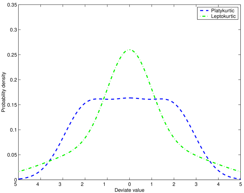
To demonstrate this point, we simulate non-Gaussian noise according to two models — one strongly leptokurtic and one strongly platykurtic — and apply the coincidence and Gaussian-approximation maximum likelihood tests described in sections IV D 1 and IV D 2 to calculate the relationship between detection efficiency and false alarm fraction for a fixed signal. A convenient model for a stationary non-Gaussian noise process is the mixture Gaussian. A mixture Gaussian distribution has the form

$\displaystyle P\left(x|\{p_{i},\mu_{i},\sigma_{i},i=1\ldots N\}\right)$ $\displaystyle=$ $\displaystyle\sum_{i=1}^{N}p_{i}{\exp\left[{(x-\mu_{i})^{2}/2\sigma_{i}^{2}}\right]\over\sqrt{2\pi}\sigma_{i}}$ (121)
$\displaystyle\sum_{i=1}^{N}p_{i}$ $\displaystyle=$ $\displaystyle 1$ (122)
$\displaystyle p_{i}$ $\displaystyle>$ $\displaystyle 0.$ (123)

By appropriate choice of the constants $p_{i}$, $\mu_{i}$ and $\sigma_{i}$ a mixture Gaussian can approximate any uncorrelated noise distribution through its first $2N$ moments.

The two distributions we model here are drawn from the mixture Gaussian distributions described in table IV. The corresponding probability distribution functions are shown graphically in figure 3. Note that each is strongly non-Gaussian, though in different ways.

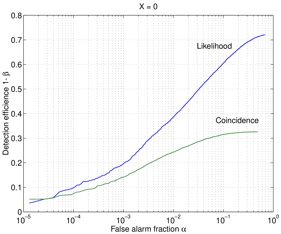
Figures 4 and 5 show the detection efficiency as a function of the false alarm frequency for the coincidence and Gaussian-approximation maximum likelihood tests for the leptokurtic distribution and platykurtic distributions, respectively. The detection efficiency and false alarm fractions were determined by Monte Carlo simulations. The signal parameters used in the detection efficiency simulations are given in the second and third columns of table III. The conclusion reached earlier — that the maximum likelihood test is superior to the coincidence test — is not sensitive to the approximation of Gaussian noise. There is no qualitative difference between figures 4, 5, and 2, which summarize the relative characteristics of these two tests when the noise is strongly non-Gaussian or Gaussian. In all cases the detection efficiency of the (Gaussian-approximation) maximum likelihood test is less than that of the coincidence test at the same false alarm fraction. The principal reason for this superior performance is the same here as in the case of Gaussian noise: the response of two or more detectors to incident radiation is correlated, and the Gaussian-approximation maximum likelihood test is sensitive to the expected inter-detector cross-correlations, reducing the S/N when the correlations are not consistent with waves from the same source.

V Conclusions

The output of several gravitational wave detectors can be combined, in a form of aperture synthesis, to form a single, more sensitive gravitational wave detector. Here we describe such an analysis, based on the likelihood function, appropriate to the detection of a burst gravitational wave source, of known waveform, in a network of gravitational wave detectors. This likelihood analysis of the joint output of several detectors leads to the optimal matched filter for the output of the multi-detector network.

The analysis presented here stands in contrast to “coincidence” analyses, where the output of each detector is studied separately to arrive at a list of events, which are then compared between the detectors to determine if there are any coincidences, which may be taken to be evidence for gravitational waves.

The critical difference between these two analyses is that the likelihood is sensitive to the coherent response of the detector network to the incident signal. This leads the likelihood based analysis to have greater discriminating power than a coincidence analysis, as shown by a greater detection efficiency to false alarm frequency ratio.

The importance of inter-detector correlations is clearly important when looking for a signal; however, it is also important when the noise in two or more detectors is correlated. Such correlations are naturally accommodated in the optimal filter developed here; however, they cannot be naturally accommodated in a coincidence analysis which, by its very nature, ignores inter-detector correlations.

The likelihood function derived here begins with an assumption that the detector noise is Gaussian-stationary; however, the results obtained are much more general. We show that treating non-Gaussian as if it were Gaussian is, in a very well-defined sense, the most appropriate choice if the only available characterization of the noise is through its mean and correlation function. While it is sometimes claimed [12] that coincidence is the only reasonable test when the noise is non-Gaussian, we show in a series of numerical simulations that the even when the noise is strongly non-Gaussian the likelihood test, treating the noise as if it were Gaussian, outperforms the coincidence test as measured by the ratio of detection efficiency to false alarm fraction.

A naive estimate of the computational cost of computing the matched filter for a network of detectors might suggest that the cost is proportional to the cube of the length of the time series and the number of detectors. If the calculation is properly organized, however, the cost is seen to be strictly proportional to the duration of the signal being sought and no more than the square of the number of detectors in the network.

The work described here can be considered aperture synthesis specialized to the problem of searching for signals of finite duration whose waveform is known. The problem of searching for stochastic signals remains to be studied. True aperture synthesis — searching for fringes in the interfered output of several gravitational wave detectors — may well be the most sensitive means of searching for the truly unanticipated source and is a particularly promising direction for future research.

Acknowledgements.
I am especially grateful to Joseph Romano for a very careful reading of early versions of this manuscript and to Albert Lazzarini for pointing out that the likelihood can always be made to separate. This work was supported by grants from the Alfred P. Sloan Foundation and the National Science Foundation (PHY 93-08728, PHY 98-00111 and PHY 99-96213).

REFERENCES

  • [1] H. Lück et al., in Gravitational Waves, No. 523 in AIP Conference Proceedings, edited by S. Meshkov (American Institute of Physics, Melville, New York, 2000), pp. 119–127, proceedings of the Third Edoardo Amaldi Conference. See Ref. [28].
  • [2] M. Coles, in Gravitational Waves, No. 523 in AIP Conference Proceedings, edited by S. Meshkov (American Institute of Physics, Melville, New York, 2000), proceedings of the Third Edoardo Amaldi Conference. See Ref. [28].
  • [3] F. Marion, in Gravitational Waves, No. 523 in AIP Conference Proceedings, edited by S. Meshkov (American Institute of Physics, Melville, New York, 2000), pp. 110–118, proceedings of the Third Edoardo Amaldi Conference. See Ref. [28].
  • [4] L. Conti et al., in Gravitational Waves, No. 523 in AIP Conference Proceedings, edited by S. Meshkov (American Institute of Physics, Melville, New York, 2000), proceedings of the Third Edoardo Amaldi Conference. See Ref. [28].
  • [5] A. de Waard and G. Frossati, in Gravitational Waves, No. 523 in AIP Conference Proceedings, edited by S. Meshkov (American Institute of Physics, Melville, New York, 2000), proceedings of the Third Edoardo Amaldi Conference. See Ref. [28].
  • [6] D. Blair, in Gravitational Waves, No. 523 in AIP Conference Proceedings, edited by S. Meshkov (American Institute of Physics, Melville, New York, 2000), proceedings of the Third Edoardo Amaldi Conference. See Ref. [28].
  • [7] L. S. Finn, Phys. Rev. D 46, 5236 (1992).
  • [8] L. S. Finn and D. F. Chernoff, Phys. Rev. D 47, 2198 (1993).
  • [9] C. Cutler and É. É. Flanagan, Phys. Rev. D 49, 2658 (1994).
  • [10] P. Jaranowski and A. Krolak, Phys. Rev. D 49, 1723 (1994).
  • [11] P. Jaranowski, K. D. Kokkotas, A. Królak, and G. Tsegas, Class. Quantum Grav. 13, 1279 (1996).
  • [12] J. Creighton, Phys. Rev. D 60, 021101 (1999).
  • [13] S. Bose, S. V. Dhurandhar, and A. Pai, Pramana 53, 1125 (1999).
  • [14] S. Bose, A. Pai, and S. Dhurandhar, Int. J. Mod. Phys. D 9, 325 (2000).
  • [15] A. V. Oppenheim and R. W. Schafer, Discrete-Time Signal Processing, Prentice Hall signal processing series (Prentice-Hall, Englewood Cliffs, New Jersey, 1989).
  • [16] W. L. Briggs and V. E. Henson, The DFT: An owner’s manual for the Discrete Fourier Transform (SIAM, Philadelphia, 1995).
  • [17] K. Tsubono, in First Edoardo Amaldi Conference on Gravitational Wave Experiments, edited by E. Coccia, G. Pizzella, and F. Ronga (World Scientific, Singapore, 1995), p. 112.
  • [18] W. O. Hamilton et al., in Omnidirectional Gravitational Radiation Observatory, edited by W. F. V. Jr., O. D. Aguiar, and N. S. Magalhaes (World Scientific, Singapore, 1997), pp. 19–26.
  • [19] M. Cerdonio et al., Class. Quantum Grav. 14, 1491 (1997).
  • [20] P. Astone et al., Phys. Rev. D 47, 362 (1993).
  • [21] P. Astone et al., Astroparticle Physics 7, 231 (1997).
  • [22] G. J. Feldman and R. D. Cousins, Phys. Rev. D 57, 3873 (1998).
  • [23] C. Giunti, Phys. Rev. D 59, 053001 (1999).
  • [24] C. Giunti, Phys. Rev. D 59, 113009 (1999).
  • [25] B. P. Roe and M. B. Woodroofe, Phys. Rev. D 60, 053009 (1999).
  • [26] H. V. Poor, An Introduction to Signal Detection and Estimation, Springer texts in electrical engineering, 2nd ed. (Springer-Verlag, New York, 1994).
  • [27] L. Ljung, System Identification: Theory for the User, Information and system sciences, 2nd ed. (Prentice Hall, Upper Saddle River, New Jersey, 1999).
  • [28] Gravitational Waves, No. 523 in AIP Conference Proceedings, edited by S. Meshkov (American Institute of Physics, Melville, New York, 2000), proceedings of the Third Edoardo Amaldi Conference.
Functions Sequences
Time Domain Frequency Domain Time Domain Frequency Domain
Scalar $a(t)$ $\widetilde{a}(f)$ ${a}[k]$ $\widetilde{a}[k]$
Vector $\mathchoice{{\hbox{\boldmath$\displaystyle a$}}}{{\hbox{\boldmath$\textstyle a$}}}{{\hbox{\boldmath$\scriptstyle a$}}}{{\hbox{\boldmath$\scriptscriptstyle a$}}}(t)$ $\widetilde{\mathchoice{{\hbox{\boldmath$\displaystyle a$}}}{{\hbox{\boldmath$\textstyle a$}}}{{\hbox{\boldmath$\scriptstyle a$}}}{{\hbox{\boldmath$\scriptscriptstyle a$}}}}(f)$ ${\mathchoice{{\hbox{\boldmath$\displaystyle a$}}}{{\hbox{\boldmath$\textstyle a$}}}{{\hbox{\boldmath$\scriptstyle a$}}}{{\hbox{\boldmath$\scriptscriptstyle a$}}}}[k]$ $\widetilde{\mathchoice{{\hbox{\boldmath$\displaystyle a$}}}{{\hbox{\boldmath$\textstyle a$}}}{{\hbox{\boldmath$\scriptstyle a$}}}{{\hbox{\boldmath$\scriptscriptstyle a$}}}}[k]$
Matrix $\mathchoice{{\hbox{\boldmath$\displaystyle A$}}}{{\hbox{\boldmath$\textstyle A$}}}{{\hbox{\boldmath$\scriptstyle A$}}}{{\hbox{\boldmath$\scriptscriptstyle A$}}}(t)$ $\widetilde{\mathchoice{{\hbox{\boldmath$\displaystyle A$}}}{{\hbox{\boldmath$\textstyle A$}}}{{\hbox{\boldmath$\scriptstyle A$}}}{{\hbox{\boldmath$\scriptscriptstyle A$}}}}(f)$ ${\mathchoice{{\hbox{\boldmath$\displaystyle A$}}}{{\hbox{\boldmath$\textstyle A$}}}{{\hbox{\boldmath$\scriptstyle A$}}}{{\hbox{\boldmath$\scriptscriptstyle A$}}}}[k]$ $\widetilde{\mathchoice{{\hbox{\boldmath$\displaystyle A$}}}{{\hbox{\boldmath$\textstyle A$}}}{{\hbox{\boldmath$\scriptstyle A$}}}{{\hbox{\boldmath$\scriptscriptstyle A$}}}}[k]$
TABLE I.: Nomenclature.
Detector separation $(2R)$ $25/f_{0}$
Sampling frequency $4f_{0}$
Detector noise PSD ($S_{\pm}$) $1/f_{0}$
Observation duration ($T_{D}$) $100/f_{0}$
TABLE II.: Parameters describing the toy receiver and signal duration used for examples in this paper. All parameters are given in units of $f_{0}$, the reciprocal signal duration.
Gaussian Leptokurtic Platykurtic
$A_{0}$ 2.5 3.5 3.0
$X_{0}$ 0.0 0.0 0.0
TABLE III.: Parameters describing the signal used in the example calculation of the detection efficiency for the Gaussian, platykurtic and leptokurtic noise examples.
Leptokurtic Platykurtic
$p$ $(1/2,1/4,1/4)$ $(61/192,131/384,131/384)$
$\mu$ $(0,2,-2)$ $(0,2,-2)$
$\sigma$ $(1,2,2)$ $(1,1,1)$
Mean: 0 0
Std. Dev.: 2.1213 1.9311
TABLE IV.: Parameters describing the two mixture Gaussian models used to explore the maximum likelihood and coincidence test performance non-Gaussian noise in section IV E. Also shown are the mean and standard deviation of the distributions. The corresponding PDFs are shown graphically in figure 3.
Refer to caption
FIG. 1.: To illustrate the effectiveness of a correlation analysis compared to a coincidence analysis we apply both to a model problem involving two identical detectors of isotropic response. The detectors are denoted $+$ and $-$. Their relative separation and the parameters describing the direction of an incident plane wave signal are shown in this figure.
Refer to caption
FIG. 2.: The false alarm frequency $\alpha$ vs. the detection efficiency ($1-\beta$) for the maximum likelihood and coincidence tests in the presence of Gaussian noise. The parameters describing the signal, to which the detection efficiency refers, are given in the first column of table III. Note that the performance of the maximum likelihood test is everywhere superior to the performance of the coincidence test. The degree of superiority will vary with signal strength; however, the relativity performance of the two tests will not. The superior performance of the likelihood based test is attributable to the way in which the maximum likelihood test internalizes the detector-detector correlations that are present when a real signal interacts with the receiver. For more details see section IV D 3.
Refer to caption
FIG. 3.: The probability distribution functions for the leptokurtic and platykurtic non-Gaussian noise models used to test the relative performance of the coincidence and Gaussian-approximation likelihood test. For more details see table IV and section IV E.
Refer to caption
FIG. 4.: The false alarm fraction $\alpha$ vs. the detection efficiency ($1-\beta$) for the Gaussian-approximation likelihood and coincidence tests in the presence of strongly leptokurtic non-Gaussian noise. The noise is described by the mixture Gaussian model whose parameters are given in the first column of table IV and the signal used for calculating the detection efficiency is described in table III. Figure 3 shows the noise PDF graphically. Note that, even though when noise is substantially non-Gaussian, the Gaussian-approximation likelihood test has significantly better performance then the coincidence test. The superiority is attributable to the fact that real signals are correlated between the detectors, and the Gaussian approximation likelihood test, even when the noise is not Gaussian, is still sensitive to those correlations. For more discussion see section IV E.
Refer to caption
FIG. 5.: The false alarm fraction $\alpha$ vs. the detection efficiency ($1-\beta$) for the Gaussian-approximation likelihood and coincidence tests in the presence of strongly platykurtic non-Gaussian noise. The noise is described by the mixture Gaussian model whose parameters are given in table IV and whose PDF is shown graphically in figure 3. For more discussion see section IV E.