An effective model of the spacetime foam

Abstract

An approximate model of the spacetime foam is offered in which each quantum handle (wormhole) is a 5D wormhole-like solution. A spinor field is introduced for an effective description of this foam. The topological handles of the spacetime foam can be attached either to one space or connect two different spaces. In the first case we have a wormhole with the quantum throat and such object can demonstrate a model of preventing the formation the naked singularity with relation $e>m$. In the second case the spacetime foam looks as a dielectric with quantum handles as dipoles. It is supposed that supergravity theories with a nonminimal interaction between spinor and electromagnetic fields can be considered as an effective model approximately describing the spacetime foam.

1 Introduction

The notion of a spacetime foam was introduced by Wheeler [1, 2] for the description of the possible complex structure of the spacetime on the Planck scale ($L_{Pl}\approx 10^{-33}cm$). This hypothesized spacetime foam is a set of quantum wormholes (WH) (handles) appearing in the spacetime on the Planck scale level (see Fig.1).

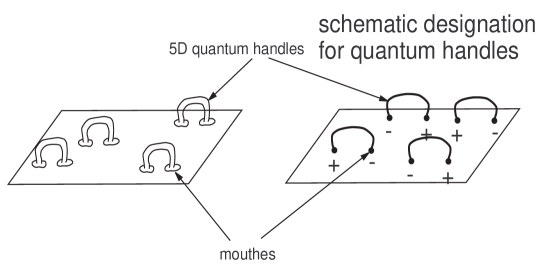
Figure 1: At the left side of the figure is presented a hypothesized spacetime foam. If we neglect of the cross section of handle then (at the right) hand we have a schematic designation for the spacetime foam.

For the macroscopic observer these quantum fluctuations are smoothed and we have an ordinary smooth manifold with the metric submitting to Einstein equations. The exact mathematical description of this phenomenon is very difficult and even though there is a doubt: does the Feynman path integral in the gravity contain a topology change of the spacetime ? This question spring up because (according to the Morse theory) the singular points must arise by the topology change. In such points the time arrow is undefined that leads in difficulties at definition of the Lorentzian metric, curvature tensor and so on. The main goal of this paper is to submit an effective model of the spacetime foam.

2 Model of a single quantum wormhole

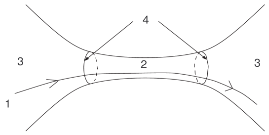
Figure 2: Here whole spacetime is 5D but in the external spacetime (3) $G_{55}$ is nonvariable and we have Kaluza-Klein theory in its initial interpretation as 4D gravity + electromagnetism. In the throat (2) $G_{55}$ component of the 5D metric is equivalent to 4D gravity+electromagnetism+scalar field. Near the event horizon (4) the metric is the Reissner-Nordstrom metric and the throat is a solution of the 5D Kaluza-Klein theory. We should join these metrics on the event horizons. (1) is the force line of the electric field.

At first we present a model of a single handle in the spacetime foam, see Fig(2). The 5D metric [3, 4, 5] for the throat is

$$ds^{2} = \eta_{AB}\omega^{A}\omega^{B}=$$ (1)

$$-\frac{r_{0}^{2}}{\Delta(r)}(d\chi-\omega(r)dt)^{2}+\Delta(r)dt^{2}-dr^{2}-$$

$$a(r)\left(d\theta^{2}+\sin\theta^{2}d\varphi^{2}\right),$$

$$a = r^{2}_{0}+r^{2},\quad\Delta=\pm\frac{2r_{0}}{q}\frac{r^{2}+r_{0}^{2}}{r^{2}-r_{0}^{2}},\quad$$ (2)

$$\omega=\pm\frac{4r_{0}^{2}}{q}\frac{r}{r^{2}-r_{0}^{2}}.$$

where $\chi$ is the 5^th extra coordinate; $\eta_{AB}=(\pm,-,-,-,\mp)$, $A,B=0,1,2,3,5$; $r,\theta,\varphi$ are the $3D$ polar coordinates; $r_{0}>0$ and $q$ are some constants. We can see that there are two closed $ds^{2}_{(5)}(\pm r_{0})=0$ hypersurfaces at the $r=\pm r_{0}$. In some sense these hypersurfaces are like to the event horizon and in Ref.[6] such hypersurfaces are named as a $D$-holes. On these hypersurfaces we should join [7]:

• the flux of the 4D electric field (defined by the Maxwell equations) with the flux of the 5D electric field defined by $R_{5t}=0$ Kaluza-Klein equation.

• the area of the Reissner-Nordström event horizon with the area of the $ds^{2}_{(5)}(\pm r_{0})=0$ hypersurface.

It is necessary to note that both solutions (Reissner-Nordström black hole and 5D throat) have only two integration constants and on the event horizon takes place an algebraic relation between these 4D and 5D integration constants. Another explanation of the fact that we use only two joining condition is the following (see Ref.[8] for the more detailed explanations): in some sense on the event horizon holds a “holography principle”. This means that in the presence of the event horizon the 4D and 5D Einstein equations lead to a reduction of the amount of initial data. For example the Einstein - Maxwell equations for the Reissner-Nordström metric

$$ds^{2} = \Delta dt^{2}-\frac{dr^{2}}{\Delta}-r^{2}\left(d\theta^{2}+\sin^{2}d\varphi^{2}\right),$$ (3)

$$A_{\mu} = \left(\omega,0,0,0)\right)$$ (4)

(where $A_{\mu}$ is the electromagnetic potential, $\kappa$ is the gravitational constant) can be written as

$$-\frac{\Delta^{\prime}}{r}+\frac{1-\Delta}{r^{2}} = \frac{\kappa}{2}{\omega^{\prime}}^{2},$$ (5)

$$\omega^{\prime} = \frac{q}{r^{2}}.$$ (6)

For the Reissner - Nordström black hole the event horizon is defined by the condition $\Delta(r_{g})=0$, where $r_{g}$ is the radius of the event horizon. Hence in this case we see that on the event horizon

$$\Delta^{\prime}_{g}=\frac{1}{r_{g}}-\frac{\kappa}{2}r_{g}{\omega^{\prime}_{g}}^{2},$$ (7)

here (g) means that the corresponding value is taken on the event horizon. Thus, Eq. (5), which is the Einstein equation, is a first-order differential equations in the whole spacetime $(r\geq r_{g})$. The condition (7) tells us that the derivative of the metric on the event horizon is expressed through the metric value on the event horizon. This is the same what we said above: the reduction of the amount of initial data takes place by such a way that we have only two integration constants (mass $m$ and charge $e$ for the Reissner-Nordström solution and $q$ and $r_{0}$ for the 5D throat).

The 5D throat has an interesting property [9]. We see that the signs of the $\eta_{55}$ and $\eta_{00}$ are not defined. We remark that this 5D metric is located behind the event horizon therefore the 4D observer is not able to determine the signs of the $\eta_{55}$ and $\eta_{00}$. Moreover this 5D metric can fluctuate between these two possibilities. Hence the external 4D observer is forced to describe such composite WH by means of something like spinor.

Another interesting characteristic property of this solution is that we have the flux of electric field through the throat, i.e. each mouth can entrap the electric force lines and this leads that this mouth is like to electric charge for the external 4D observer, see Fig.3.

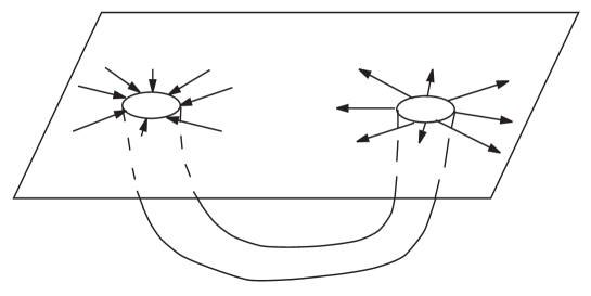
Figure 3: The left mouth of the quantum WH entraps the force lines of the electric field and looks as (-) electric charge. The force lines outcome from the right mouth of WH which one looks as (+) charge.

We can neglect the cross section of the throat and in this case each mouth is point-like and we can try to describe these mouthes with help of some effective field. Taking into account the spinor-like properties of quantum handles, we assume that spacetime foam can be described with help of an effective spinor field.

3 Approximate model of the spacetime foam

The physical meaning of the spinor field depends on the method of attaching the quantum handles to the external space, see Fig.(4).

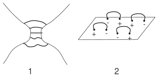
Figure 4: At the left hand of the figure quantum handles connect two spaces. At the right hand the mouthes of quantum handles are separated in distance of the order $l_{Pl}$.

3.1 Quantum wormholes with separated mouthes

In this case $|\psi|^{2}$ is a density of the mouthes in the external space and $e|\psi|^{2}$ is a density of the electric charge [10].

Following this way we write differential equations for the gravitational + electromagnetic fields in the presence of the spacetime foam $(\psi)$ as follows

$$R_{\mu\nu}-\frac{1}{2}g_{\mu\nu}R = T_{\mu\nu},$$ (8)

$$\left(i\gamma^{\mu}\partial_{\mu}+eA_{\mu}-\frac{i}{4}\omega_{\bar{a}\bar{b}\mu}\gamma^{\mu}\gamma^{[\bar{a}}\gamma^{\bar{b}]}-m\right)\psi = 0,$$ (9)

$$D_{\nu}F^{\mu\nu}=4\pi e\left({\bar{\psi}}\gamma^{\mu}\psi\right),$$ (10)

For our model we use the following ansatz: the spherically symmetric metric

$$ds^{2}=e^{2\nu(r)}\Delta(r)dt^{2}-\frac{dr^{2}}{\Delta(r)}-r^{2}\left(d\theta^{2}+\sin^{2}d\varphi^{2}\right),$$ (11)

the electromagnetic potential

$$A_{\mu}=\left(-\phi,0,0,0\right),$$ (12)

and the spinor field

$$\tilde{\psi}=e^{-i\omega t}\frac{e^{-\nu/2}}{r\Delta^{1/4}}\left(f,0,ig\cos\theta,ig\sin\theta e^{i\varphi}\right).$$ (13)

The following is very important for us: the ansatz (13) for the spinor field $\psi$ has the $T_{t\varphi}$ component of the energy-momentum tensor and the $J^{\varphi}=4\pi e(\bar{\psi}\gamma^{\varphi}\psi)$ component of the current. Let we remind that $\psi$ determines the stochastical gas of the virtual WH’s which can not have a preferred direction in the spacetime. This means that after substitution expression (11)-(13) into field equations they should be averaged by the spin direction of the ansatz (13). After this averaging we have $T_{t\varphi}=0$ and $J^{\varphi}=0$ and we have the following equations system describing our spherically symmetric spacetime

$$f^{\prime}\sqrt{\Delta} = \frac{f}{r}-g\left(\left(\omega-e\phi\right)\frac{e^{-\nu}}{\sqrt{\Delta}}+m\right),$$ (14)

$$g^{\prime}\sqrt{\Delta} = f\left(\left(\omega-e\phi\right)\frac{e^{-\nu}}{\sqrt{\Delta}}-m\right)-\frac{g}{r},$$ (15)

$$r\Delta^{\prime} = 1-\Delta-\kappa\frac{e^{-2\nu}}{\Delta}\left(\omega-e\phi\right)\left(f^{2}+g^{2}\right)-r^{2}e^{-2\nu}{\phi^{\prime}}^{2},$$ (16)

$$r\Delta\nu^{\prime} = \kappa\frac{e^{-2\nu}}{\Delta}\left(\omega-e\phi\right)\left(f^{2}+g^{2}\right)-\kappa\frac{e^{-\nu}}{r\sqrt{\Delta}}fg-$$ (17)

$$\frac{\kappa}{2}m\frac{e^{-\nu}}{\sqrt{\Delta}}\left(f^{2}-g^{2}\right),$$

$$r^{2}\Delta\phi^{\prime\prime} = -8\pi e\left(f^{2}+g^{2}\right)-\left(2r\Delta-r^{2}\Delta\nu^{\prime}\right)\phi^{\prime},$$ (18)

where $\kappa$ is some constant. This equations system was investigated in [11] and result is the following. A particle-like solution exists which has the following expansions near $r=0$

$$f(r) = f_{1}r+{\cal O}(r^{2}),\quad g(r)={\cal O}(r^{2}),$$ (19)

$$\Delta(r) = 1+{\cal O}(r^{2}),\quad\nu(r)={\cal O}(r^{2}),\quad\phi(r)={\cal O}(r^{2})$$ (20)

and the following asymptotical behaviour

$$\Delta(r) \approx 1-\frac{2m_{\infty}}{r}+\frac{(2e_{\infty})^{2}}{r^{2}},\quad\nu(r)\approx const,$$ (21)

$$\phi(r) \approx \frac{2e_{\infty}}{r},$$ (22)

$$f \approx f_{0}e^{-\alpha r},\quad g\approx g_{0}e^{-\alpha r},$$

$$\frac{f_{0}}{g_{0}} = \sqrt{\frac{m_{\infty}+\omega}{m_{\infty}-\omega}},\quad\alpha^{2}=m_{\infty}^{2}-\omega^{2},$$ (23)

where $m_{\infty}$ is the mass for the observer at infinity and $2e_{\infty}$ is the charge of this solution.

The solution exists for both cases $(|e_{\infty}|/m_{\infty})>1$ and $(|e_{\infty}|/m_{\infty})<1$ but for us is essential the first case with $(|e_{\infty}|/m_{\infty})>1$. In this case the classical Einstein-Maxwell theory leads to the “naked” singularity. The presence of the spacetime foam drastically changes this result: the appearance of the virtual wormholes can prevent the formation of the “naked” singularuty in the Reissner-Nordström solution with $|e|/m>1$.

Our interpretation of this solution is presented on the Fig.(5).

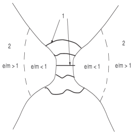
Figure 5: 1 are the quantum (virtual) WHs, 2 are two solutions with $|e_{\infty}|/m_{\infty}>1$. Such object can be named as the wormhole with quantum throat.

3.2 Quantum wormholes with non-separated mouthes

The second possibitiy [12] is presented on the Fig.(6).

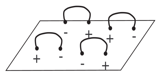
Figure 6: The distance between mouthes of the quantum handle is of order $l_{Pl}$.

We will consider the 5D Kaluza-Klein theory + torsion + spinor field. The Lagrangian in this case is

$${\cal L} = \sqrt{-G}\left\{-\frac{1}{2k}\left(R^{(5)}-S_{ABC}S^{ABC}\right)+\right.$$ (24)

$$\left.\frac{\hbar c}{2}\left[i\bar{\psi}\left(\gamma^{C}\nabla_{C}-\frac{mc}{i\hbar}\right)\psi+h.c.\right]\right\}$$

where $\nabla_{C}=\partial_{C}-\frac{1}{4}(\omega_{\bar{A}\bar{B}C}+S_{\bar{A}\bar{B}C})\gamma^{[\bar{A}}\gamma^{\bar{B}]}$ is the covariant derivative, $G$ is the determinant of the 5D metric, $R^{(5)}$ is the 5D scalar curvature, $S_{ABC}$ is the antisymmetrical torsion tensor, $A,B,C$ are the 5D world indexes, $\bar{A},\bar{B},\bar{C}$ are the 5-bein indexes, $\gamma^{B}=h^{B}_{\bar{A}}\gamma^{\bar{A}}$, $h^{B}_{\bar{A}}$ is the 5-bein, $\gamma^{\bar{A}}$ are the 5D $\gamma$ matrixes with usual definitions $\gamma^{\bar{A}}\gamma^{\bar{B}}+\gamma^{\bar{B}}\gamma^{\bar{A}}=2\eta^{\bar{A}\bar{B}}$, $\eta^{\bar{A}\bar{B}}=(+,-,-,-,-)$ is the signature of the 5D metric, $\psi$ is the spinor field which effectively and approximately describes the spacetime foam, $[]$ means the antisymmetrization, $\hbar$, $c$ and $m$ are the usual constants. After dimensional reduction we have

$${\cal L}=\sqrt{-g}\left\{-\frac{1}{2k}\left(R+\frac{1}{4}F_{\alpha\beta}F^{\alpha\beta}\right)+\right.$$

$$\left.\frac{\hbar c}{2}\left[i\bar{\psi}\left(\gamma^{\mu}\tilde{\nabla}_{\mu}-\frac{1}{8}F_{\bar{\alpha}\bar{\beta}}\gamma^{\bar{5}}\gamma^{[\bar{\alpha}}\gamma^{\bar{\beta}]}-\right.\right.\right.$$

$$\left.\left.\left.\frac{1}{4}l^{2}_{Pl}\left(\gamma^{[\bar{A}}\gamma^{\bar{B}}\gamma^{\bar{C}]}\right)\left(i\bar{\psi}\gamma_{[\bar{A}}\gamma_{\bar{B}}\gamma_{\bar{C}]}\psi\right)-\frac{mc}{i\hbar}\right)\psi+h.c.\right]\right\}$$ (25)

$$S^{\bar{A}\bar{B}\bar{C}}=2l^{2}_{Pl}\left(i\bar{\psi}\gamma^{[\bar{A}}\gamma^{\bar{B}}\gamma^{\bar{C}]}\psi\right)$$ (26)

where $g$ is the determinant of the 4D metric, $\tilde{\nabla}_{\mu}=\partial_{\mu}-\frac{1}{4}\omega_{\bar{a}\bar{b}\mu}\gamma^{[\bar{a}}\gamma^{\bar{b}]}$ is the 4D covariant derivative of the spinor field without torsion, $R$ is the 4D scalar curvature, $F_{\alpha\beta}=\partial_{\alpha}A_{\beta}-\partial_{\beta}A_{\alpha}$ is the Maxwell tensor, $A_{\mu}=h^{\bar{5}}_{\mu}$ is the electromagnetic potential, $\alpha,\beta,\mu$ are the 4D world indexes, $\bar{\alpha},\bar{\beta},\bar{\mu}$ are the 4D vier-bein indexes, $h^{\bar{\mu}}_{\nu}$ is the vier-bein, $\gamma^{\bar{\mu}}$ are the 4D $\gamma$ matrixes with usual definitions $\gamma^{\bar{\mu}}\gamma^{\bar{\nu}}+\gamma^{\bar{\nu}}\gamma^{\bar{\mu}}=2\eta^{\bar{\mu}\bar{\nu}}$, $\eta^{\bar{\mu}\bar{\nu}}=(+,-,-,-)$ is the signature of the 4D metric. Varying with respect to $g_{\mu\nu}$, $\bar{\psi}$ and $A_{\mu}$ leads to the following equations

$$R_{\mu\nu}-\frac{1}{2}g_{\mu\nu}R=\frac{1}{2}\left(-F_{\mu\alpha}F_{\nu}^{\alpha}+\frac{1}{4}g_{\mu\nu}F_{\alpha\beta}F^{\alpha\beta}\right) +$$

$$4l^{2}_{Pl}\left[\left(i\bar{\psi}\gamma_{\mu}\tilde{\nabla}_{\nu}\psi+i\bar{\psi}\gamma_{\nu}\tilde{\nabla}_{\mu}\psi\right)+h.c.\right] -$$

$$2l^{2}_{Pl}\left[F_{\mu\alpha}\left(i\bar{\psi}\gamma^{\bar{5}}\gamma_{[\nu}\gamma^{\alpha]}\psi\right)+F_{\nu\alpha}\left(i\bar{\psi}\gamma^{\bar{5}}\gamma_{[\mu}\gamma^{\alpha]}\psi\right)\right] -$$

$$2g_{\mu\nu}l^{4}_{Pl}\left(i\bar{\psi}\gamma^{[\bar{A}}\gamma^{\bar{B}}\gamma^{\bar{C}]}\psi\right)\left(i\bar{\psi}\gamma_{[\bar{A}}\gamma_{\bar{B}}\gamma_{\bar{C}]}\psi\right)$$ , (27)

$$D_{\nu}H^{\mu\nu}=0,\,H^{\mu\nu}=F^{\mu\nu}+\tilde{F}^{\mu\nu}$$ ,

$$\tilde{F}^{\mu\nu}=4l^{2}_{Pl}\left(i\bar{\psi}\gamma^{\bar{5}}\gamma^{[\mu}\gamma^{\nu]}\psi\right)=4l^{2}_{Pl}E^{\mu\nu\alpha\beta}\left(i\bar{\psi}\gamma_{[\alpha}\gamma_{\beta]}\psi\right)$$ , (28)

$$i\gamma^{\mu}\tilde{\nabla}_{\mu}\psi-\frac{1}{8}F_{\bar{\alpha}\bar{\beta}}\left(i\gamma^{\bar{5}}\gamma^{[\bar{\alpha}}\gamma^{\bar{\beta}]}\psi\right) -$$

$$\frac{1}{2}l^{2}_{Pl}\left(i\gamma^{[\bar{A}}\gamma^{\bar{B}}\gamma^{\bar{C}]}\psi\right)\left(i\bar{\psi}\gamma_{[\bar{A}}\gamma_{\bar{B}}\gamma_{\bar{C}]}\psi\right) = 0,$$ (29)

where $\omega_{\bar{a}\bar{b}\mu}$ is the 4D Ricci coefficients without torsion, $E^{\mu\nu\alpha\beta}$ is the 4D absolutely antisymmetric tensor. The most interesting for us is the Maxwell equation (28) which permits us to discuss the physical meaning of the spinor field. We would like to show that this equation in the given form is similar to the electrodynamic in the continuous media. Let we remind that for the electrodynamic in the continuous media two tensors $\bar{F}^{\mu\nu}$ and $\bar{H}^{\mu\nu}$ are introduced [13] for which we have the following equations system (in the Minkowski spacetime)

$$\bar{F}_{\alpha\beta,\gamma}+\bar{F}_{\gamma\alpha,\beta}+\bar{F}_{\beta\gamma,\alpha} = 0,$$ (30)

$$\bar{H}^{\alpha\beta}_{,\beta} = 0$$ (31)

and the following relations between these tensors

$$\bar{H}_{\alpha\beta}u^{\beta} = \varepsilon\bar{F}_{\alpha\beta}u^{\beta},$$ (32)

$$\bar{F}_{\alpha\beta}u_{\gamma}+\bar{F}_{\gamma\alpha}u_{\beta}+\bar{F}_{\beta\gamma}u_{\alpha} = \mu\left(\bar{H}_{\alpha\beta}u_{\gamma}+\bar{H}_{\gamma\alpha}u_{\beta}+\bar{H}_{\beta\gamma}u_{\alpha}\right)$$ (33)

where $\varepsilon$ and $\mu$ are the dielectric and magnetic permeability respectively, $u^{\alpha}$ is the 4-vector of the matter. For the rest media and in the 3D designation we have

$$\varepsilon\bar{E}_{i} = \bar{E}_{i}+4\pi\bar{P}_{i}=\bar{D}_{i},\quad\mbox{where}\quad\bar{E}_{i}=\bar{F}_{0i},\quad\bar{D}_{0i}=\bar{H}_{0i},$$ (34)

$$\mu\bar{H}_{i} = \bar{H}_{i}+4\pi\bar{M}_{i}=\bar{B}_{i},\quad\mbox{where}\quad\bar{B}_{i}=\epsilon_{ijk}\bar{F}^{jk},\quad\bar{H}_{i}=\epsilon_{ijk}\bar{H}^{jk},$$ (35)

where $P_{i}$ is the dielectric polarization and $M_{i}$ is the magnetization vectors, $\epsilon_{ijk}$ is the 3D absolutely antisymmetric tensor. Comparing with the (28) Maxwell equation for the spacetime foam in the 3D form

$$E_{i}+\tilde{E}_{i} = D_{i}\quad\mbox{where }\quad E_{i}=F_{0i},\quad\tilde{E}_{i}=\tilde{F}_{0i},\quad D_{i}=H_{0i}$$ (36)

$$B_{i}+\tilde{B}_{i} = H_{i}\quad\mbox{where}\;B_{i}=\epsilon_{ijk}F^{jk},\;\tilde{B}_{i}=\epsilon_{ijk}\tilde{F}^{jk},\;H_{i}=\epsilon_{ijk}H^{jk}$$ (37)

we see that the following notations can be introduced.

$$\tilde{E}_{i}=4l^{2}_{Pl}\epsilon_{ijk}\left(i\bar{\psi}\gamma^{[j}\gamma^{k]}\psi\right)$$ (38)

is the polarization vector of the spacetime foam and

$$\tilde{B}_{i}=-4l^{2}_{Pl}\epsilon_{ijk}\left(i\bar{\psi}\gamma^{\bar{5}}\gamma^{[j}\gamma^{k]}\psi\right)$$ (39)

is the magnetization vector of the spacetime foam.

The physical reason for this is evidently: each quantum WH is like to a moving dipole (see Fig.(7) which produces microscopical electric and magnetic fields.

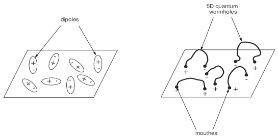
Figure 7: For the 4D observer each mouth looks as a moving electric charge. This allows us in some approximation imagine the spacetime foam as a continuous media with a polarization.

4 Supergravity as a possible model of the spacetime foam

From the above-mentioned arguments we see that the most important for such kind models of the spacetime foam is the presence of the nonminimal interaction term (in Lagrangian) between spinor and electromagnetic fields. Let we note that the N=2 supergravity [14] which contains the vier-bein $e^{a}_{\mu}$, Majorana Rarita-Schwinger field $\psi_{\mu}$, photon $A_{\mu}$ and a second Majorana spin-$\frac{3}{2}$ field $\varphi_{\mu}$ has the following term in Lagrangian

$${\cal L}_{se} = \frac{\kappa}{\sqrt{2}}\bar{\psi}_{\mu}\left(eF^{\mu\nu}+\frac{1}{2}\gamma_{5}\tilde{F}^{\mu\nu}\right)\varphi_{\nu}+\cdots,$$

$$\quad\tilde{F}_{\mu\nu} = e_{\mu\nu\alpha\beta}F^{\alpha\beta}$$ (40)

The term like this usually occur in supergravities which have some gauge multiplet of supergravity and some matter multiplet. Taking into account the previous reasonings we can suppose that supergravity theories can be considered as approximate models of the spacetime foam.

5 Conclusions

Thus, here we have proposed the approximate model for the description of the spacetime foam. This model is based on the assumption that the whole spacetime is 5 dimensional but $G_{55}$ is the dynamical variable only in the quantum topological handles (wormholes). In this case 5D gravity has the solution which we have used as a model of the single quantum wormhole. The properties of this solution is such that we can assume that the quantum topological handles (wormholes) can be approximately described by some effective spinor field.

The topological handles of the spacetime foam either can be attached to one space or connect two different spaces. In the first case we have something like to strings between two $D$-branes (or wormhole with the quantum throat) and such object can demonstrate a model of preventing the formation the naked singularity with relation $e>m$. In the second case the spacetime foam looks as a dielectric with quantum handles as dipoles.

Such model leads to the very interesting experimental consequences. We see that the spacetime foam has 5D structure and it connected with the electric field. This observation allows us to presuppose that the very strong electric field can open a door into 5 dimension! The question is: as is great should be this field ? The electric field $E_{i}$ in the CGSE units and $e_{i}$ in the “geometrized” units can be connected by formula

$$e_{i} = \frac{G^{1/2}}{c^{2}}E_{i}=\left(2.874\times 10^{-25}\;cm^{-1}/gauss\right)E_{i},$$ (41)

$$\left[e_{i}\right] = cm^{-1},\quad\left[E_{i}\right]=V/cm$$ (42)

As we see the value of $e_{i}$ is defined by some characteristic length $l_{0}$. It is possible that $l_{0}$ is a length of the $5^{th}$ dimension. If $l_{0}=l_{Pl}$ then $E_{i}\approx 10^{57}V/cm$ and this field strength is in the Planck region, and is will beyond experimental capabilities to create. But if $l_{0}$ has a different value it can lead to much more realistic scenario for the experimental capability to open door into $5^{th}$ dimension.

Another interesting conclusion of this paper is that supergravity theories having nonminimal interaction between spinor and electromagnetic fileds can be considered as approximate and effective models of the spacetime foam.

6 Acknowledgment

I would like to acknowledze the generosity of NATO in its support for this workshop and ICTP (grant KR-154).

References

• [1] C. Misner and J. Wheeler, Ann. of Phys., 2, 525 (1957); J. Wheeler, Ann. of Phys., 2, 604(1957).
• [2] J. Wheeler, Neutrinos, Gravitation and Geometry (Princeton Univ. Press, 1960).
• [3] A. Chodos and S. Detweiler, Gen. Rel. Grav. 14 (1982) 879-890.
• [4] G. ClΓ©ment, Gen. Rel. Grav. 16 (1984) 477-489; G. ClΓ©ment, Gen. Rel. Grav. 16 (1984) 131-138.
• [5] V. Dzhunushaliev, Grav. Cosmol., 3, 240(1997).
• [6] Bronnikov K., Int.J.Mod.Phys. D4, 491(1995), Grav. Cosmol., 1, 67(1995).
• [7] V. Dzhunushaliev, Mod. Phys. Lett. A 13, 2179 (1998).
• [8] V. Dzhunushaliev, β€œMatching condition on the event horizon and the holography principle”, gr-qc/9907086, to be published in Int. J. Mod. Phys. D.
• [9] V. Dzhunushaliev, H.-J.Schmidt, Grav. Cosmol. 5, 187 (1999).
• [10] V. Dzhunushaliev, β€œWormhole with Quantum Throat”, gr-qc/0005008, to be published in Grav. Cosmol.
• [11] F.Β Finster, J.Β Smoller, S.-T.Β Yau, Phys. Lett. A259, 431 (1999).
• [12] V. Dzhunushaliev, β€œAn Approximate Model of the Spacetime Foam”, gr-qc/0006016.
• [13] L.D. Landau and E.M. Lifshitz, β€œElectrodynamics of Continuous Media”, (Pergamon Press, Oxford - London - New Jork - Paris, 1960).
• [14] S. Ferrara and P.Β V. Nieuwenhuizen, Phys. Rev. Lett. 37, 1669 (1976).