Action and Energy of the Gravitational Field

Abstract

We present a detailed examination of the variational principle for metric general relativity as applied to a “quasilocal” spacetime region ${\cal M}$ (that is, a region that is both spatially and temporally bounded). Our analysis relies on the Hamiltonian formulation of general relativity, and thereby assumes a foliation of ${\cal M}$ into spacelike hypersurfaces $\Sigma$. We allow for near complete generality in the choice of foliation. Using a field–theoretic generalization of Hamilton–Jacobi theory, we define the quasilocal stress-energy-momentum of the gravitational field by varying the action with respect to the metric on the boundary $\partial{\cal M}$. The gravitational stress-energy-momentum is defined for a two–surface $B$ spanned by a spacelike hypersurface in spacetime. We examine the behavior of the gravitational stress-energy-momentum under boosts of the spanning hypersurface. The boost relations are derived from the geometrical and invariance properties of the gravitational action and Hamiltonian. Finally, we present several new examples of quasilocal energy–momentum, including a novel discussion of quasilocal energy–momentum in the large-sphere limit towards spatial infinity. Chapel Hill and Raleigh, April 2002

I Introduction

Beginning with the earliest days of general relativity and continuing to the present, relativists have actively sought to define gravitational stress-energy-momentum (sem) from a variational principle. The motivation to do so is readily apparent. sem, and energy in particular, plays a central role in most branches of physics. In this paper we discuss a relatively new approach (see for example¹ Refs. [1, 2, 3, 4, 5, 6, 7, 8, 9, 10, 11, 12, 13, 14, 15, 16, 17, 18, 19, 20, 21, 22, 23, 24, 25]) to the problem, which we refer to here as the canonical quasilocal formalism (cqf). The cqf is based upon a field–theoretic generalization of Hamilton–Jacobi theory. We present many results new to the cqf and, in the process, recover the recent results from Refs. [12, 18].

Over the last thirty years, research has yielded a more–or–less satisfactory understanding of total energy–momentum for asymptotically flat spacetimes and asymptotically anti-de Sitter spacetimes. However, as no physical system is ever truly isolated, these asymptotic conditions—however useful—are ultimately unphysical, theoretical idealizations. In any case, practical numerical calculations are always restricted to a spatially finite region. For this reason and others (see the next paragraph), recent efforts have turned to the issue of defining sem quasilocally, that is to say, associating gravitational sem with spatially bounded regions. (Indeed, one direct application of the formalism we present here is an approach to numerical outer boundary conditions for the gravitational field described in a forthcoming paper.[26])

As we will see, the cqf naturally leads to a definition of gravitational sem that is quasilocal. We are motivated primarily by the desire to obtain physically meaningful and useful energy–like quantities that characterize the classical gravitational field in a bounded region. However, our original motivation for developing the cqf stemmed from a problem in semiclassical gravity, namely, understanding thermodynamical internal energy for black holes. The asymptotically–defined Arnowitt-Deser-Misner (adm) energy[27], for example, cannot serve as a useful internal energy because an infinite, self-gravitating system at finite temperature is thermodynamically unstable. Thus, the partition function can be defined only for systems with finite spatial extent, and this necessitates a quasilocal definition of energy (see Refs [28, 29, 30, 8, 31, 32, 33, 34] and references therein).

Before turning to the cqf, let us mention several approaches toward defining gravitational energy from a variational principle. The history of this problem is long, so an encompassing study would require a separate, extensive review. Here, we give only a brief summary of several of the historically important works. These works are based on a field–theoretic generalization of Noether’s theorem [35].

Einstein was the first to derive gravitational sem from an action principle.[36] By discarding a metric–dependent divergence term in the second–order covariant Hilbert action, he obtained a first–order action, the so–called $\Gamma\Gamma$ action, that is the four–integral of a bulk Lagrangian quadratic in the Christoffel symbols. He then carried out a Noether–type analysis, and derived a canonical gravitational sem pseudotensor and its corresponding super–potential.² Given what we’ve learned about the asymptotic structure of spacetime in the decades since this early work, it is remarkable how successful the Einstein definitions were.[37] Most of the key properties of spatial infinity (including decay of the metric and derivatives of the metric) are found in Einstein’s original paper. The drawback of Einstein’s approach is that the $\Gamma\Gamma$ action is not fully diffeomorphism invariant (it is invariant modulo boundary terms), and his gravitational sem is coordinate dependent. At the quasilocal level there is no obvious general prescription for how one should choose coordinates.

In the early 1960’s Møller discovered a new bulk action for general relativity that is similar to Einstein’s $\Gamma\Gamma$ action, but is quadratic in the tetrad connection (Ricci rotation) coefficients.[39] We might refer to it as the $\omega\omega$ action. Like the Einstein Lagrangian, the Møller bulk Lagrangian differs from the Hilbert Lagrangian by a pure divergence. (See also related work in Refs. [40, 41, 42].) Although the Møller action is not fully invariant under “internal” transformations of the tetrad, it is diffeomorphism invariant and is therefore arguably preferable to the Einstein action as the starting point for a Noether–type analysis. Moreover, the resulting theory of sem can be translated readily into the language of two–spinors, a powerful formalism which has led to numerous results in the quasilocal setting (see, for instance, the works of Szabados, Refs. [43, 44, 45, 46] and references therein). We point out, however, that in adopting the Møller action, one is departing from pure metric relativity, Einstein’s original theory. It is not clear at all that the sem concepts derived in any such framework “pull back” to the metric phase space.

By introducing a background metrical structure, one may isolate—in a coordinate independent fashion—a purely metric divergence term in the Hilbert action. In Ref. [47] Rosen discarded such a term, thereby obtaining another bulk action amenable to Noether techniques. An invocation of the Noether theorem in purely metric gravity, this approach towards defining gravitational sem is close in spirit to Einstein’s, and may be considered as a a refined version of his original analysis. However, the approach would seem limited in that there is not always a natural choice of background spacetime. Bičák, Lynden-Bell, Katz, and Petrov have developed and used an improved version of the approach in several recent papers (see Refs. [48, 49, 50] and references therein) addressing, among other things, gravitational perturbations of cosmological solutions to the Einstein equations.

We now turn to the canonical quasilocal formalism. Our analysis is based on the so-called “Trace-K” action[51, 1, 2, 3], which differs from the standard Hilbert action by metric-dependent boundary terms. Its use leads to a purely metric formalism, as does the Einstein $\Gamma\Gamma$ action. However, unlike the $\Gamma\Gamma$ action, the Trace-K action³ is manifestly invariant under coordinate transformations. Moreover, the Trace-K action does not depend on any background structures.⁴ Since the Trace-K action does not stem from a bulk Lagrangian, it is not immediately clear how to apply the Noether theorem. But we can bypass a Noether analysis altogether, using instead the cqf which is based on Hamilton-Jacobi theory. We point out that our approach is intimately related to a body of work done by Kijowski and co-workers (see Ref. [52] and references therein). Kijowski’s approach starts with novel and important ideas from symplectic theory [53], and examines the relevant symplectic geometry in great detail. Our approach, on the other hand, starts with standard Hamilton-Jacobi theory and focuses primarily on the physical spacetime geometry. We stress that both approaches are merely different faces of a Hamiltonian analysis, and thus somewhat different from more traditional approaches based on Noether techniques.

Consider a spatially and temporally bounded spacetime region ${\cal M}$ with metric $g_{\mu\nu}$ and boundary $\partial{\cal M}$. The boundary $\partial{\cal M}$ of the region consists of a timelike element ${\bar{\cal T}}$ (the meaning of the “bar” is explained below) and spacelike elements $\Sigma^{\prime}$ and $\Sigma^{\prime\prime}$. Such a spacetime region is depicted in Fig. 1, but note that ${\bar{\cal T}}$ need not be connected.

FIG. 1.:

We assume that the spacetime ${\cal M}$ is foliated into spacelike hypersurfaces $\Sigma$, defined by $t={\rm const}$. Further, we require the boundary of each $\Sigma$ leaf to lie in ${\bar{\cal T}}$.⁵ The intersections of the leaves of the spacetime foliation $\Sigma$ with the timelike boundary element ${\bar{\cal T}}$ define a foliation of ${\bar{\cal T}}$ into two–dimensional spacelike hypersurfaces $B$ (which need not be connected). The region ${\cal M}$ may itself be contained in some ambient spacetime. We note that the boundary $B$ and its history ${\bar{\cal T}}$ are simply submanifolds of spacetime and need not be physical barriers.

The future–pointing unit normal to the $t={\rm const}$ hypersurfaces is denoted $u^{\mu}$, and the outward–pointing unit normal of ${\bar{\cal T}}$ is denoted ${\bar{n}}^{\mu}$. The induced metric on $\Sigma$ is $h_{ij}$ and the induced metric on ${\bar{\cal T}}$ is ${\bar{\gamma}}_{ij}$. Because in general ${\bar{n}}^{\mu}u_{\mu}\neq 0$ on ${\bar{\cal T}}$, the Eulerian observers of the $B$ foliation of ${\bar{\cal T}}$, comoving with ${\bar{\cal T}}$, need not be at rest with respect to the $\Sigma$ slices. This necessitates the “barred” and “unbarred” notation which keeps track of the two sets of Eulerian observers at the boundary: those comoving with ${\bar{\cal T}}$ and at rest with respect to the $B$ foliation of ${\bar{\cal T}}$ (the “barred observers”) and those at rest with respect to the $\Sigma$ foliation of ${\cal M}$ (the “unbarred observers”).

The four–velocities of the barred observers will be denoted ${\bar{u}}^{\mu}$. Similarly, at each point of ${\bar{\cal T}}$, we define $n^{\mu}$ as the unit outward pointing vector for the unbarred observers. That is, $n^{\mu}$ lies in $\Sigma$ and is orthogonal to $B$.⁶ Note that, by construction, ${\bar{u}}^{\mu}{\bar{n}}_{\mu}=0$ and $u^{\mu}n_{\mu}=0$. These vectors are related by the boost relations

$${\bar{n}}_{\mu} = \gamma n_{\mu}+\gamma vu_{\mu}\ ,$$ ()

$${\bar{u}}_{\mu} = \gamma u_{\mu}+\gamma vn_{\mu}\ .$$ ()

where $v$ is the boost velocity between the two sets of observers and $\gamma=(1-v^{2})^{-1/2}$. In Appendix A we present the details of the kinematical relationships needed for this paper.

As mentioned, our analysis is carried out in the purely metric formulation of gravity and is based on the Trace K action,[51, 2, 3, 17]

$$S[g]=\frac{1}{2\kappa}\int_{{\cal M}}d^{4}x\sqrt{-g}\,{{\Re}}+\frac{1}{\kappa}\int_{\Sigma^{\prime}}^{\Sigma^{\prime\prime}}d^{3}x\sqrt{h}\,K-\frac{1}{\kappa}\int_{{\bar{\cal T}}}d^{3}x\sqrt{-{\bar{\gamma}}}\,{\bar{\Theta}}-\frac{1}{\kappa}\int^{B^{\prime\prime}}_{B^{\prime}}d^{2}x\sqrt{\sigma}\theta\ .$$ (2)

Here, $\kappa$ is $8\pi$ times Newton’s constant. For simplicity we have omitted matter and cosmological constant contributions to the action. The symbol $\int_{\Sigma^{\prime}}^{\Sigma^{\prime\prime}}$ is shorthand for $\int_{\Sigma^{\prime\prime}}-\int_{\Sigma^{\prime}}$, and $K$ is the trace of the extrinsic curvature $K_{\mu\nu}=-h_{\mu}^{\alpha}\nabla_{\alpha}u_{\nu}$ of the boundary elements $\Sigma^{\prime}$ and $\Sigma^{\prime\prime}$. Similarly, the function ${\bar{\Theta}}$ is the trace of the extrinsic curvature ${\bar{\Theta}}_{\mu\nu}=-{\bar{\gamma}}_{\mu}^{\alpha}\nabla_{\alpha}{\bar{n}}_{\nu}$ of the boundary element ${\bar{\cal T}}$. The action (2) includes contributions (first considered in Refs. [2, 3]) from the “corners” $B^{\prime}=\Sigma^{\prime}\cap{\bar{\cal T}}$ and $B^{\prime\prime}=\Sigma^{\prime}\cap{\bar{\cal T}}$, where $\sigma$ is the determinant of the metric $\sigma_{ab}$ on the corners. The velocity parameter $\theta$ is defined by $\sinh\theta=-u^{\mu}{\bar{n}}_{\mu}=\gamma v$.

The Trace-K action has the crucial property that its associated variational principle features fixation of the induced three metric ${}^{3}g_{ij}$ on $\partial{\cal M}$.⁷ In particular, the lapse of proper time for an observer, comoving with ${\bar{\cal T}}$ and at rest with the $B$ foliation, is fixed as boundary data since this information is encoded in the fixed $\bar{\cal T}$ three–metric. The value of the quasilocal energy surface density (at a given point on the observer’s worldline) is defined through a hj variation as minus the rate of change of the classical action with respect to an infinitesimal stretch (enacted at the given point) in the proper time separation between $\Sigma^{\prime}$ and $\Sigma^{\prime\prime}$. Of course, the $\bar{\cal T}$ three–metric specifies more than just the lapse of proper time between the initial and final slices—it contains information about all possible spacetime intervals on $\bar{\cal T}$. One is free to consider the changes in the classical action corresponding to arbitrary hj variations in the $\bar{\cal T}$ metric. The original Ref. [1] has demonstrated how this freedom leads not only to the energy surface density but also to surface densities for tangential momentum and spatial stress (both are pointwise–defined $B$ tensors).

In this paper, we extend the cqf analysis of Ref.[1] by considering changes in the classical action corresponding to hj variations in $\Sigma^{\prime\prime}$ (or $\Sigma^{\prime}$) boundary data. This leads to quasilocal surface densities for normal momentum, tangential momentum (which is equivalent to the previous definition), and temporal stress (this was also shown in Ref. [12]). Therefore, the quasilocal stress-energy-momentum consists of energy, normal momentum, and tangential momentum surface densities and spatial and temporal stress tensors.

We also extend the cqf by considering “boost relations” between the quasilocal surface densities as defined by barred and unbarred observers. These sem boost relations can be viewed as canonical realizations of the relations (() ‣ I) satisfied by the barred and unbarred observers’ unit vectors. The observer dependence of the quasilocal sem is best described from the following perspective. The various sem quantities are defined as tensors on the spatial boundary $B$ spanned by a spacelike hypersurface $\Sigma$. The boost relations characterize the behavior of these tensors under a boost of the spanning slice $\Sigma$; that is, they characterize the dependence of the quasilocal sem on the choice of observers passing through $B$. As purely geometrical relations, the boost relations among energy, tangential momentum, and normal momentum surface densities have been noted elsewhere in the literature (see, for instance, Refs. [43, 52]). Moreover, their particular role in the cqf has been pointed out in Refs. [5, 12]. Here we present a unique derivation of these relations, demonstrating that their geometrical content is already encoded in the gravitational Hamiltonian.

Finally, we present several new examples of quasilocal energy–momentum, including an analysis of cylindrical gravitational waves. We also include a novel discussion of quasilocal energy–momentum in the large-sphere limit towards spatial infinity. Agreement between the Trautman–Bondi–Sachs total graviational energy–momentum and the notion of quasilocal energy–momentum arising in the cqf has been considered elsewhere.[16]

In Sec. II we prepare for the Hamilton–Jacobi variation of the Trace-K action by considering the general variation of the Hilbert action. Of particular importance are the corner terms that arise at the intersections of $\bar{\cal T}$ with $\Sigma^{\prime}$ and $\Sigma^{\prime\prime}$. These terms have appeared previously in the literature.[2, 3, 12, 52] However, to our knowledge, Sec. II contains the first completely geometrical derivation of the result (although the same result was obtained explicitly via another method in Ref. [52]). In Sec. III we apply the cqf to the Trace-K action and derive the quasilocal sem. In the process, we obtain the boost relations among the energy and momentum surface densities and spatial and temporal stress tensors as defined by the boosted and unboosted observers. We also discuss the notion of boost invariants which allow for the construction of several mass definitions which have appeared in the relativity literature. Section IV contains a derivation of the Hamiltonian form of the action and its variation. We then derive the boost relations for the energy and momentum surface densities by boosting the gravitational Hamiltonian. Finally, Sec. V and Sec. VI deal with concrete examples and applications, and in these sections we chose units such that the constant $\kappa$ appearing in Eq. (2) is simply $8\pi$. In Sec. V we first deal with the issue of zero–points for the quasilocal densities, and the relationship between these zero-points and a freedom always present in any variational principle. The freedom concerns appending to the action, here the gravitational Trace-K action, an arbitrary functional of the fixed boundary data. Having (at least partially) dealt with this issue, we then write down quasilocal energy and momentum expressions for a variety of exact solutions to the Einstein equations; and in Sec. VI we apply our formalism to spacetimes with are asymptotically flat in spacelike directions, in the process making some novel observations about total gravitational energy at spatial infinity.

Appendix A contains several key kinematical results that are used throughout the paper. Appendix B is devoted to the derivation of certain curvature splittings needed for the analysis in Sec. III. Finally, in Appendix C, we show that the rate of change of the boost parameter equals the normal gradient of the lapse function defining the boost. This is needed for the analysis in Sec. IV.

II Variation of the Hilbert action

In this section we consider the standard Hilbert action,[54]

$$S_{\scriptscriptstyle H}[g]=\frac{1}{2\kappa}\int_{\cal M}d^{4}x\sqrt{-g}{\,}\Re{\,},$$ (3)

and its associated variational principle as applied to a bounded spacetime region ${\cal M}$, a careful analysis of which is crucial for the entire discussion. Such an analysis is, of course, not new[51, 2, 3, 17, 18, 52]; however, as we do give a new version of a nontrivial calculation of fundamental importance, we believe the details belong up front and not relegated to an appendix.

The relevant geometry of the various foliations of ${\cal M}$ is described in the Introduction and Appendix A. We examine the variation $\delta S_{\scriptscriptstyle H}$ of the action induced by an infinitesimal variation $\delta g_{\mu\nu}$ in the metric tensor and derive the following result:[51, 2, 3, 17, 18, 52]

$$\delta S_{\scriptscriptstyle H}=-\frac{1}{2\kappa}\int_{\cal M}d^{4}x\sqrt{-g}G^{\mu\nu}\delta g_{\mu\nu}-\int^{\Sigma^{\prime\prime}}_{\Sigma^{\prime}}d^{3}xh_{ij}\delta P^{ij}-\int_{\bar{\cal T}}d^{3}x\bar{\gamma}_{ij}\delta\bar{\Pi}{}^{ij}+\frac{1}{\kappa}\int^{B^{\prime\prime}}_{B^{\prime}}d^{2}x\sqrt{\sigma}\delta\theta{\,}.$$ (4)

In this expression $G^{\mu\nu}$ is the Einstein tensor, $\theta$ is the velocity parameter described earlier, and

$$P^{ij} = \frac{\sqrt{h}}{2\kappa}\left(Kh^{ij}-K^{ij}\right)$$ ()

$$\bar{\Pi}^{ij} = -\frac{\sqrt{-\bar{\gamma}}}{2\kappa}\left(\bar{\Theta}\bar{\gamma}{}^{ij}-\bar{\Theta}{}^{ij}\right)$$ ()

are respectively the $\Sigma$ and ${\bar{\cal T}}$ gravitational momenta.

In writing the Hilbert action (3) and its variation (4), we do not necessarily assume that the spacetime boundary elements $\Sigma^{\prime}$, $\Sigma^{\prime\prime}$, and ${\bar{\cal T}}$ have smooth embeddings in ${\cal M}$. That is, the unit normal ${\bar{n}}^{\mu}$ of ${\bar{\cal T}}$ and the unit normals $u^{\mu}$ of $\Sigma^{\prime}$ and $\Sigma^{\prime\prime}$ need not be continuous vector fields. For example, the timelike boundary element ${\bar{\cal T}}$ can contain a “kink”, a spacelike two-surface at which ${\bar{n}}^{\mu}$ changes discontinuously. In that case the ${\bar{\cal T}}$ boundary term in $\delta S_{\scriptscriptstyle H}$ contains a contribution from the kink. The form of the contribution is discussed in Ref. [6].

A Preliminary results and a lemma

To begin, let us collect a few results concerning the variation $\delta\Gamma^{\lambda}{}_{\mu\nu}$ of the affine connection induced by an infinitesimal $\delta g_{\mu\nu}$. With these we prove a lemma of particular use when examining the variation $\delta S_{\scriptscriptstyle H}$ of the action.⁸ First, expansion of the identity $\delta(\nabla_{\lambda}g_{\mu\nu})=0$ leads directly to the result

$$2\delta\Gamma_{(\mu\nu)\lambda}=\nabla_{\lambda}\delta g_{\mu\nu}{\,}.$$ (6)

Second, the well–known formula[54] $\delta\Re_{\mu\nu}=\nabla_{\lambda}\delta\Gamma^{\lambda}{}_{\mu\nu}-\nabla_{\nu}\delta\Gamma^{\lambda}{}_{\mu\lambda}$ for the induced variation of the Ricci tensor implies that the contracted variation $g^{\mu\nu}\delta\Re_{\mu\nu}$ is a pure spacetime divergence. Indeed, writing $g^{\mu\nu}\delta\Re_{\mu\nu}=\nabla_{\mu}V^{\mu}$, we find that

$$V^{\mu}=2\delta\Gamma^{[\mu\nu]}{}_{\nu}{\,}.$$ (7)

Finally, consider a metric–dependent covector $\omega_{\mu}$ (i. e. $\delta\omega_{\mu}$ need not vanish) and the spacetime divergence $\nabla_{\mu}\omega^{\mu}$ constructed from it. The variation of this divergence is

$$\delta\nabla_{\mu}\omega^{\mu}=-{\textstyle\frac{1}{2}}\omega_{\mu}V^{\mu}+\nabla^{\mu}\delta\omega_{\mu}-{\textstyle\frac{1}{2}}(\nabla^{\mu}\omega^{\nu})\delta g_{\mu\nu}-{\textstyle\frac{1}{2}}\nabla^{\mu}(\omega^{\nu}\delta g_{\mu\nu}){\,}.$$ (8)

To obtain this result, expand the variation $\delta(g^{\mu\nu}\nabla_{\mu}\omega_{\nu})$, insert the identity $\delta\nabla_{\mu}\omega_{\nu}=\nabla_{\mu}\delta\omega_{\nu}-\omega_{\lambda}\delta\Gamma^{\lambda}{}_{\mu\nu}$, and then use Eqs. (6) and (7).

We now prove the following.
lemma: Consider a unit hypersurface–orthogonal vector field, say $u^{\mu}$ with normalization $u^{\mu}u_{\mu}=\epsilon$ (with $\epsilon=\pm 1$).⁹ Also consider the induced metric $h_{\mu\nu}=g_{\mu\nu}-\epsilon u_{\mu}u_{\nu}$ on the hypersurfaces to which $u^{\mu}$ is orthogonal, as well as the extrinsic curvature tensor $K_{\mu\nu}=-h^{\alpha}_{\mu}\nabla_{\alpha}u_{\nu}$. The variation $\delta K$ of the mean curvature $K=-\nabla_{\mu}u^{\mu}$ satisfies the equation

$$2\delta K=u_{\mu}V^{\mu}-K^{\mu\nu}\delta h_{\mu\nu}-D_{\alpha}(h^{\alpha}_{\mu}\delta u^{\mu}){\,},$$ (9)

where $D_{\alpha}$ is the covariant derivative operator compatible with $h_{\mu\nu}$.

Our proof of the lemma makes use of the following two identities: (i) $\nabla^{\mu}u^{\nu}=-K^{\mu\nu}+\epsilon u^{\mu}u^{\lambda}\nabla_{\lambda}u^{\nu}$ and (ii) $\delta u_{\mu}={\textstyle\frac{1}{2}}\epsilon u_{\mu}u^{\alpha}u^{\beta}\delta g_{\alpha\beta}$. Identity (i) follows directly from the definition of $K_{\mu\nu}$ and the spacetime expression for the induced metric $h_{\mu\nu}$. We verify (ii) by writing $u_{\mu}=\epsilon N\nabla_{\mu}t$, where the coordinate $t$ labels the hypersurfaces to which $u_{\mu}$ is orthogonal and $N=(\epsilon\nabla_{\mu}t{\,}g^{\mu\nu}{\,}\nabla_{\nu}t)^{-1/2}$ is the lapse function. As the first step towards proving the lemma, we rewrite Eq. (8) with $u_{\mu}$ in place of $\omega_{\mu}$, make substitutions with the identities (i) and (ii), and do a bit of algebra in order to obtain

$$2\delta K=u_{\mu}V^{\mu}-K^{\mu\nu}\delta g_{\mu\nu}-\epsilon(\nabla_{\lambda}u^{\lambda})u^{\mu}u^{\nu}\delta g_{\mu\nu}+h^{\mu\lambda}\nabla_{\lambda}(u^{\nu}\delta g_{\mu\nu}){\,}.$$ (10)

Now, by (i) $\nabla_{\mu}u^{\mu}=h^{\mu\nu}\nabla_{\mu}u_{\nu}$; and, therefore, we may collect the last two terms on the right–hand side in Eq. (10), thereby arriving at

$$2\delta K=u_{\mu}V^{\mu}-K^{\mu\nu}\delta g_{\mu\nu}+h^{\lambda\kappa}\nabla_{\lambda}(h^{\mu}_{\kappa}u^{\nu}\delta g_{\mu\nu}){\,}.$$ (11)

Finally, since $K^{\mu\nu}$ is purely spatial, $K^{\mu\nu}\delta g_{\mu\nu}=K^{\mu\nu}\delta h_{\mu\nu}$. Moreover, with identity (ii) we can show that $h^{\mu}_{\kappa}u^{\nu}\delta g_{\mu\nu}=-h_{\mu\kappa}\delta u^{\mu}$. Substitution of these results along with the definition of $D_{\alpha}$ into Eq. (11) completes the proof.

As we have been careful to allow for the case $\epsilon=1$, our proof of the lemma establishes

$$2\delta\bar{\Theta}=\bar{n}_{\mu}V^{\mu}-\bar{\Theta}^{\mu\nu}\delta\bar{\gamma}_{\mu\nu}-\bar{\cal D}_{\alpha}(\bar{\gamma}{}^{\alpha}_{\mu}\delta\bar{n}{}^{\mu})$$ (12)

as a corollary. Here, $\bar{\cal D}_{\alpha}$ is the covariant derivative compatible with the $\bar{\cal T}$ metric $\bar{\gamma}_{ij}$.

B Variation of the action

Our goal now is to obtain the expression (4) for the variation $\delta S_{\scriptscriptstyle H}$ of the Hilbert action. Simple manipulations show that the variation of the action is

$$\delta S_{\scriptscriptstyle H}=\frac{1}{2\kappa}\int_{\cal M}d^{4}x\sqrt{-g}\left(-G^{\mu\nu}\delta g_{\mu\nu}+\nabla_{\mu}V^{\mu}\right){\,},$$ (13)

where $V^{\mu}$ has been defined in Eq. (7). Focus attention on the divergence term in Eq. (13), namely,

$$(\delta S_{\scriptscriptstyle H})_{\partial{\cal M}}=\frac{1}{2\kappa}\int_{\cal M}d^{4}x\sqrt{-g}\nabla_{\mu}V^{\mu}{\,}.$$ (14)

Via Stokes’ theorem,[55]

$$\int_{\cal M}(\nabla_{\mu}V^{\mu}){\boldmath\mbox{$\epsilon$}}=\int_{\partial{\cal M}}(V\cdot{\boldmath\mbox{$\epsilon$}}){\,},$$ (15)

we can express $(\delta S_{\scriptscriptstyle H})_{\partial{\cal M}}$ as a pure boundary term. In Eq. (15) we have used abstract notation for both the spacetime volume form $({\boldmath\mbox{$\epsilon$}})_{\mu\nu\lambda\kappa}=\epsilon_{\mu\nu\lambda\kappa}$ and the three–form $(V\cdot{\boldmath\mbox{$\epsilon$}})_{\nu\lambda\kappa}=V^{\mu}\epsilon_{\mu\nu\lambda\kappa}$. The integral on the right–hand side of Eq. (15) can be written as a sum of separate integrals over each element of the boundary $\partial{\cal M}=\Sigma^{\prime}\bigcup\Sigma^{\prime\prime}\bigcup\bar{\cal T}$. Indeed, no corner-term contributions (i. e. two-surface integrals over $B^{\prime}$ and $B^{\prime\prime}$) can arise at this stage, because both $B^{\prime}$ and $B^{\prime\prime}$ are sets of measure zero with respect to $\partial{\cal M}$ and the integrand $(V\cdot{\boldmath\mbox{$\epsilon$}})$ is continuous (as both $V^{\mu}$ and $\epsilon_{\mu\nu\lambda\kappa}$ are continuous). Now, standard convention fixes the orientation of the boundary $\partial{\cal M}$ by choosing the outward–pointing normal ${\sf n}{}^{\mu}$ to $\partial{\cal M}$ as embedded in ${\cal M}$; that is to say, the alternating tensor on $\partial{\cal M}$ is taken to be $\epsilon_{\nu\lambda\kappa}={\sf n}{}^{\mu}\epsilon_{\mu\nu\lambda\kappa}$. Subject to this convention, one finds in general that

$$\int_{\partial{\cal M}}(V\cdot{\boldmath\mbox{$\epsilon$}})=\int_{\partial{\cal M}}d^{3}x\sqrt{|{}^{3}g|}\epsilon{\sf n}_{\mu}V^{\mu}{\,}.$$ (16)

In this expression $|{}^{3}g|$ is the (absolute value of) the determinant of the induced metric on $\partial{\cal M}$ and $\epsilon={\sf n}_{\mu}{\sf n}^{\mu}$ is a sign factor which is either $1$ or $-1$ depending on the boundary element. Notice that $\epsilon{\sf n}_{\mu}$ is the covector dual to the outward–pointing normal ${\sf n}^{\mu}$. Therefore, for the case at hand with $\partial{\cal M}=\Sigma^{\prime}\bigcup\Sigma^{\prime\prime}\bigcup\bar{\cal T}$, we expand the right–hand side of Eq. (16), and obtain

$$(\delta S_{\scriptscriptstyle H})_{\partial{\cal M}}=-\frac{1}{2\kappa}\int^{\Sigma^{\prime\prime}}_{\Sigma^{\prime}}d^{3}x\sqrt{h}u_{\mu}V^{\mu}+\frac{1}{2\kappa}\int_{\bar{\cal T}}d^{3}x\sqrt{-\bar{\gamma}}\bar{n}_{\mu}V^{\mu}$$ (17)

as the promised boundary expression for the divergence term (14).

Next, combining the lemma (9) and its corollary (12) with (17), we write the divergence term as follows:

$$(\delta S_{\scriptscriptstyle H})_{\partial{\cal M}} = -\frac{1}{2\kappa}\int^{B^{\prime\prime}}_{B^{\prime}}d^{2}x\sqrt{\sigma}\left(n_{\mu}\delta u^{\mu}+\bar{u}_{\mu}\delta\bar{n}^{\mu}\right)$$ (19)

$$-\frac{1}{2\kappa}\int^{\Sigma^{\prime\prime}}_{\Sigma^{\prime}}d^{3}x\sqrt{h}(2\delta K+K^{ij}\delta h_{ij})+\frac{1}{2\kappa}\int_{\bar{\cal T}}d^{3}x\sqrt{-\bar{\gamma}}(2\delta\bar{\Theta}+\bar{\Theta}{}^{ij}\delta\bar{\gamma}_{ij}){\,}.$$

In this expression the total derivative terms in the boundary element integrals have been expressed as integrals over the corners $B^{\prime}$ and $B^{\prime\prime}$ (again via Stokes’ theorem, but now in one lower dimension). Further, for the $\Sigma^{\prime}$, $\Sigma^{\prime\prime}$ and $\bar{\cal T}$ integrals in Eq. (19) we have chosen to use indices adapted to the boundary elements rather than general spacetime indices. Now, with the momenta (() ‣ II) used in Eq. (19), the term $(\delta S_{\scriptscriptstyle H})_{\partial{\cal M}}$ becomes

$$(\delta S_{\scriptscriptstyle H})_{\partial{\cal M}}=-\frac{1}{2\kappa}\int^{B^{\prime\prime}}_{B^{\prime}}d^{2}x\sqrt{\sigma}\left(n_{\mu}\delta u^{\mu}+\bar{u}_{\mu}\delta\bar{n}^{\mu}\right)-\int^{\Sigma^{\prime\prime}}_{\Sigma^{\prime}}d^{3}xh_{ij}\delta P^{ij}-\int_{\bar{\cal T}}d^{3}x\bar{\gamma}_{ij}\delta\bar{\Pi}{}^{ij}{\,}.$$ (20)

Our remaining task is to simplify the integrals over $B^{\prime}$ and $B^{\prime\prime}$. To achieve this, recall the boost relations

$$\bar{u}{}^{\mu} = \gamma u^{\mu}+v\gamma n^{\mu}$$ ()

$$\bar{n}{}^{\mu} = \gamma n^{\mu}+v\gamma u^{\mu}$$ ()

and their inverses, derived in terms of a double foliation of spacetime in Appendix A. These can be used to write the integrand of the corner integrals as

$$n_{\mu}\delta u^{\mu}+\bar{u}_{\mu}\delta\bar{n}^{\mu}=(\bar{n}{}_{\mu}/\gamma-vu_{\mu})\delta(\bar{u}{}^{\mu}/\gamma-vn^{\mu})+(u_{\mu}/\gamma+v\bar{n}{}_{\mu})\delta(n^{\mu}/\gamma+v\bar{u}{}^{\mu}){\,}.$$ (22)

On the right–hand side of this equation, the terms proportional to $u_{\mu}\delta n^{\mu}$ vanish. This follows from the identity $u_{\mu}\delta n^{\mu}=-n^{\mu}\delta u_{\mu}$ and the fact that $u_{\mu}$ is hypersurface–orthogonal. [Thus, as seen in identity (ii) after the Eq. (9) $\delta u_{\mu}$ is proportional to $u_{\mu}$.] Likewise, we have $\bar{n}_{\mu}\delta\bar{u}{}^{\mu}=0$, since $\bar{n}_{\mu}$ is hypersurface–orthogonal. After a bit of straightforward algebra, Eq. (22) simplifies to $n_{\mu}\delta u^{\mu}+\bar{u}_{\mu}\delta\bar{n}^{\mu}=-2\gamma^{2}\delta v$. Therefore, we may now rewrite Eq. (20) as

$$(\delta S_{\scriptscriptstyle H})_{\partial{\cal M}}=\frac{1}{\kappa}\int^{B^{\prime\prime}}_{B^{\prime}}d^{2}x\sqrt{\sigma}\gamma^{2}\delta v-\int^{\Sigma^{\prime\prime}}_{\Sigma^{\prime}}d^{3}xh_{ij}\delta P^{ij}-\int_{\bar{\cal T}}d^{3}x\bar{\gamma}_{ij}\delta\bar{\Pi}{}^{ij}{\,}.$$ (23)

Combination of this result with Eq. (13) and the definition $\tanh\theta=v$ of the boost parameter yields the desired expression (4).

C Boundary terms and the diffeomorphism invariance of the Hilbert action

The Hilbert action (3) is diffeomorphism invariant. That is, the action is unchanged if the variations in the fields are given by the Lie derivative along a vector field $\xi^{\mu}$ that is tangent to the boundaries:

$$\delta S_{H} = \frac{1}{2\kappa}\int_{\cal M}d^{4}x\,{\pounds}_{\xi}(\sqrt{-g}\Re)=\frac{1}{2\kappa}\int_{\cal M}d^{4}x\nabla_{\mu}(\xi^{\mu}\sqrt{-g}\Re)$$ (24)

$$= -\frac{1}{2\kappa}\int_{\Sigma^{\prime}}^{\Sigma^{\prime\prime}}d^{3}x\sqrt{h}\,u_{\mu}\xi^{\mu}\Re+\frac{1}{2\kappa}\int_{{\bar{\cal T}}}d^{3}x\sqrt{-{\bar{\gamma}}}\,{\bar{n}}_{\mu}\xi^{\mu}\Re$$ (25)

$$= 0\ .$$ (26)

Here, we use ${\bar{n}}_{\mu}\xi^{\mu}=0$ on ${{\bar{\cal T}}}$, and $u_{\mu}\xi^{\mu}=0$ on $\Sigma^{\prime}$ and $\Sigma^{\prime\prime}$. These imply ${\bar{n}}_{\mu}\xi^{\mu}=u_{\mu}\xi^{\mu}=0$ on $B^{\prime}$ and $B^{\prime\prime}$.

Since $\delta S_{H}=0$ when $\delta$ is given by the Lie derivative, our main result Eq. (4) implies

$$0=\delta S_{H} = -\frac{1}{\kappa}\int_{\cal M}d^{4}x\sqrt{-g}\,G^{\mu\nu}\nabla_{\mu}\xi_{\nu}+\frac{1}{\kappa}\int_{B^{\prime}}^{B^{\prime\prime}}d^{2}x\sqrt{\sigma}\,\gamma^{2}\xi^{a}\partial_{a}v$$ (28)

$$-\int_{\Sigma^{\prime}}^{\Sigma^{\prime\prime}}d^{3}x\,h_{ij}{\pounds}_{\xi}P^{ij}-\int_{{\bar{\cal T}}}d^{3}x\,{\bar{\gamma}}_{ij}{\pounds}_{\xi}{\bar{\Pi}}^{ij}\,.$$

Now use the identity

$$h_{ij}{\pounds}_{\xi}P^{ij} = {\pounds}_{\xi}P-P^{ij}{\pounds}_{\xi}h_{ij}=D_{i}(P\xi^{i})-2P^{ij}D_{i}\xi_{j}$$ (29)

$$= D_{i}(P\xi^{i}-2P^{ij}\xi_{j})+2(D_{i}P^{ij})\xi_{j}\ ,$$ (30)

where $\xi^{i}$ is the pullback of $\xi^{\mu}$ to $\Sigma^{\prime}$ or $\Sigma^{\prime\prime}$. Note that the $D_{i}(P\xi^{i})$ term will vanish when integrated to the corners. Thus, the $\Sigma^{\prime}$ and $\Sigma^{\prime\prime}$ terms in (28) become

$$-\int_{\Sigma^{\prime}}^{\Sigma^{\prime\prime}}d^{3}x\,h_{ij}{\pounds}_{\xi}P^{ij}=-2\int_{\Sigma^{\prime}}^{\Sigma^{\prime\prime}}d^{3}x\,(D_{i}P^{ij})\xi_{j}+2\int_{B^{\prime}}^{B^{\prime\prime}}d^{2}x\sqrt{\sigma}\,n_{i}P^{ij}\xi_{j}/\sqrt{h}\ .$$ (31)

Similarly, we find

$$-\int_{{\bar{\cal T}}}d^{3}x\,{\bar{\gamma}}_{ij}{\pounds}_{\xi}{\bar{\Pi}}^{ij}=-2\int_{{\bar{\cal T}}}d^{3}x\,({{\bar{\cal D}}}_{i}{\bar{\Pi}}^{ij})\xi_{j}-2\int_{B^{\prime}}^{B^{\prime\prime}}d^{2}x\sqrt{\sigma}\,{\bar{u}}_{i}{\bar{\Pi}}^{ij}\xi_{j}/\sqrt{-{\bar{\gamma}}}\,,$$ (32)

whence Eq. (28) now becomes

$$0=\delta S_{H} = -\frac{1}{\kappa}\int_{\cal M}d^{4}x\sqrt{-g}(\nabla_{\mu}G^{\mu\nu})\xi_{\nu}+\int_{B^{\prime}}^{B^{\prime\prime}}d^{2}x\sqrt{\sigma}\left({\bar{\jmath}}_{a}\xi^{a}-\jmath_{a}\xi^{a}+\gamma^{2}\xi^{a}\partial_{a}v/\kappa\right)$$ (35)

$$+\int_{\Sigma^{\prime}}^{\Sigma^{\prime\prime}}d^{3}x\left(\sqrt{h}\,u_{\mu}G^{\mu\nu}\xi_{\nu}/\kappa-2(D_{i}P^{ij})\xi_{j}\right)$$

$$-\int_{{\bar{\cal T}}}d^{3}x\left(\sqrt{-{\bar{\gamma}}}\,{\bar{n}}_{\mu}G^{\mu\nu}\xi_{\nu}/\kappa+2({\bar{\cal D}}_{i}{\bar{\Pi}}^{ij})\xi_{j}\right)\ ,$$

where we have used integration by parts on the volume (${\cal M}$) integral term. Also, we have used the definitions ${\bar{\jmath}}_{a}=-2\sigma_{ai}{\bar{\Pi}}^{ij}{\bar{u}}_{j}/\sqrt{-{\bar{\gamma}}}$ and $\jmath_{a}=-2\sigma_{ai}P^{ij}n_{j}/\sqrt{h}$.

We now use the well–known result that the gravitational field contributions to the boundary momentum constraints satisfy

$${\cal H}_{i} = -2D_{j}P^{j}_{i}=-\sqrt{h}u_{\mu}G^{\mu\nu}h_{\nu i}/\kappa\ ,$$ (36)

$${\bar{\cal H}}_{i} = -2{\bar{\cal D}}_{j}{\bar{\Pi}}^{j}_{i}=\sqrt{-{\bar{\gamma}}}{\bar{n}}_{\mu}G^{\mu\nu}{\bar{\gamma}}_{\nu i}/\kappa\ .$$ (37)

Therefore the last two integrals in Eq. (35) vanish. Since the result (35) must hold for all $\xi^{\mu}$ that are tangent to the boundary, we conclude that

$$\nabla_{\mu}G^{\mu\nu}=0\ ,$$ ()

$${\bar{\jmath}}_{a}=\jmath_{a}-\frac{1}{\kappa}\partial_{a}\theta\ ,$$ ()

where $\theta$ is the velocity parameter, $v=\tanh(\theta)$. Equation (() ‣ II Ca) is, of course, the contracted Bianchi identity. Equation (() ‣ II Cb) is an identity as well. In fact, as we will see in the next section, ${\bar{\jmath}}_{a}$ and $\jmath_{a}$ are the tangential momentum densities for the barred and unbarred observers, and the identity (() ‣ II Cb) expresses the boost relationship between these quantities.

Note that this analysis can be applied to the Trace-K action as well. Indeed, any action that is diffeomorphism invariant and differs from the Hilbert action by boundary terms can be used. The reason is that the Lie variation of a boundary term will always integrate to the corners, and then vanish since $\xi^{\mu}$ is tangent to the corner.

III Quasilocal Stress-Energy-Momentum and Boost Relations

A Quasilocal quantities

Using our main result (4) for the variation of the Hilbert action, one can easily show that the variation of the Trace-K action (2) has the following boundary terms:

$$(\delta S)_{\partial{\cal M}}=\int^{\Sigma^{\prime\prime}}_{\Sigma^{\prime}}d^{3}xP^{ij}\delta h_{ij}+\int_{\bar{\cal T}}d^{3}x\bar{\Pi}{}^{ij}\delta\bar{\gamma}{}_{ij}-\frac{1}{\kappa}\int^{B^{\prime\prime}}_{B^{\prime}}d^{2}x\theta\delta\sqrt{\sigma}\ .$$ (39)

Notice that the Trace-K action features solely fixation of the induced metric on the boundary $\partial{\cal M}$. We now wish to express the ${\bar{\cal T}}$ boundary term in $\delta S$ in terms of the geometry of the $\Sigma$ slices. Start with the $(\delta S)_{{\bar{\cal T}}}$ contribution to the variation, that is

$$\int_{{\bar{\cal T}}}d^{3}x\,{\bar{\Pi}}^{ij}\delta{\bar{\gamma}}_{ij}=-\frac{1}{2\kappa}\int_{{\bar{\cal T}}}d^{3}x\sqrt{-{\bar{\gamma}}}({\bar{\Theta}}{\bar{\gamma}}^{ij}-{\bar{\Theta}}^{ij})\delta{\bar{\gamma}}_{ij}\ .$$ (40)

With an ADM splitting of the side boundary metric ${\bar{\gamma}}_{ij}$ into a lapse function ${\bar{N}}$, a shift vector ${\bar{V}}^{a}$, and a spatial metric $\sigma_{ab}$ (see Appendix A), we find

$$\delta{\bar{\gamma}}_{ij}=-\frac{2}{{\bar{N}}}{\bar{u}}_{i}{\bar{u}}_{j}\delta{\bar{N}}-\frac{2}{{\bar{N}}}\sigma_{a{\scriptscriptstyle(}i}{\bar{u}}_{j{\scriptscriptstyle)}}\delta{\bar{V}}^{a}+\sigma^{a}_{{\scriptscriptstyle(}i}\sigma^{b}_{j{\scriptscriptstyle)}}\delta\sigma_{ab}\ .$$ (41)

With this splitting of the ${\bar{\cal T}}$ metric we then obtain

$$\int_{{\bar{\cal T}}}d^{3}x\,{\bar{\Pi}}^{ij}\delta{\bar{\gamma}}_{ij}=-\frac{1}{\kappa}\int_{{\bar{\cal T}}}d^{3}x\sqrt{\sigma}\biggl{\{}({\bar{\Theta}}+ {\bar{u}}_{i}{\bar{\Theta}}^{ij}{\bar{u}}_{j})\delta{\bar{N}}+(\sigma_{ai}{\bar{\Theta}}^{ij}{\bar{u}}_{j})\delta{\bar{V}}^{a}$$ (43)

$$+\frac{{\bar{N}}}{2}({\bar{\Theta}}\sigma^{ab}-\sigma^{a}_{i}{\bar{\Theta}}^{ij}\sigma^{b}_{j})\delta\sigma_{ab}\biggr{\}}\ .$$

Now, in order to achieve our goal of expressing $(\delta S)_{{\bar{\cal T}}}$ in terms of $\Sigma$ geometry, we must find a “splitting” of the ${\bar{\cal T}}$ extrinsic curvature tensor ${\bar{\Theta}}_{ij}$. The desired expression

$${\bar{\Theta}}_{\mu\nu}=\gamma k_{\mu\nu}+\gamma v\ell_{\mu\nu}+({\bar{n}}\cdot{\bar{a}}){\bar{u}}_{\mu}{\bar{u}}_{\nu}+2\sigma^{\alpha}_{{\scriptscriptstyle(}\mu}{\bar{u}}_{\nu{\scriptscriptstyle)}}(K_{\alpha\beta}n^{\beta}-\nabla_{\alpha}\theta)\ ,$$ (44)

is derived in Appendix B. In this expression, we have used the definitions

$$k_{\mu\nu} = -\sigma^{\alpha}_{\mu}\sigma^{\beta}_{\nu}\nabla_{\alpha}n_{\beta}\ ,$$ ()

$$\ell_{\mu\nu} = -\sigma^{\alpha}_{\mu}\sigma^{\beta}_{\nu}\nabla_{\alpha}u_{\beta}\ .$$ ()

The unit normals $u^{\mu}$, $n^{\mu}$ associated with the hypersurfaces $\Sigma$ are related to the unit normals ${\bar{u}}^{\mu}$, ${\bar{n}}^{\mu}$ associated with ${\bar{\cal T}}$ as in Eqs. (() ‣ II B). Again, our conventions are that barred observers are comoving with the boundary ${\bar{\cal T}}$ while the unbarred ones are at rest in the $\Sigma$ hypersurfaces. Also in Eq. (44), ${\bar{a}}^{\mu}={\bar{u}}^{\nu}\nabla_{\nu}{\bar{u}}^{\mu}$ denotes the acceleration of the barred observers, and $K_{\alpha\beta}$ denotes the extrinsic curvature of the $\Sigma$ slices. Putting these results together, we have

$$\int_{{\bar{\cal T}}}d^{3}x\,{\bar{\Pi}}^{ij}\delta{\bar{\gamma}}_{ij}=-\frac{1}{\kappa}\int_{{\bar{\cal T}}}d^{3}x\sqrt{\sigma}\biggl{\{} [\gamma k+\gamma v\ell]\delta{\bar{N}}-[\sigma_{a}^{i}K_{ij}n^{j}-\partial_{a}\theta]\delta{\bar{V}}^{a}$$ (47)

$$-\frac{{\bar{N}}}{2}\Bigl{[}\gamma(k^{ab}-k\sigma^{ab})+{\bar{n}}\cdot{\bar{a}}\,\sigma^{ab}+\gamma v(\ell^{ab}-\ell\sigma^{ab})\Bigr{]}\delta\sigma_{ab}\biggr{\}}$$

for the ${\bar{\cal T}}$ term in the variation of the action.

The contribution to $\delta S$ from the top and bottom caps ($\Sigma^{\prime\prime}$ and $\Sigma^{\prime}$) is

$$\int^{\Sigma^{\prime\prime}}_{\Sigma^{\prime}}d^{3}x\,P^{ij}\delta h_{ij}=\frac{1}{2\kappa}\int^{\Sigma^{\prime\prime}}_{\Sigma^{\prime}}d^{3}x\sqrt{h}(Kh^{ij}-K^{ij})\delta h_{ij}\ .$$ (48)

The induced metric $h_{ij}$ can be split into a “radial” lapse function $M$, shift vector $W^{a}$, and slice metric $\sigma_{ab}$ (see Appendix A). The variation in $h_{ij}$ is then

$$\delta h_{ij}=\frac{2}{M}n_{i}n_{j}\delta M+\frac{2}{M}\sigma_{a{\scriptscriptstyle(}i}n_{j{\scriptscriptstyle)}}\delta W^{a}+\sigma^{a}_{{\scriptscriptstyle(}i}\sigma^{b}_{j{\scriptscriptstyle)}}\delta\sigma_{ab}\ ,$$ (49)

from which we obtain

$$\int^{\Sigma^{\prime\prime}}_{\Sigma^{\prime}}d^{3}x\,P^{ij}\delta h_{ij}=\frac{1}{\kappa}\int^{\Sigma^{\prime\prime}}_{\Sigma^{\prime}}d^{3}x\sqrt{\sigma}\biggl{\{}(K- n_{i}K^{ij}n_{j})\delta M-(\sigma_{ai}K^{ij}n_{j})\delta W^{a}$$ (51)

$$+\frac{M}{2}(K\sigma^{ab}-\sigma^{a}_{i}K^{ij}\sigma^{b}_{j})\delta\sigma_{ab}\biggr{\}}$$

Now use the splitting

$$K_{\mu\nu}=\ell_{\mu\nu}+(u\cdot b)n_{\mu}n_{\nu}+2\sigma^{\alpha}_{{\scriptscriptstyle(}\mu}n_{\nu{\scriptscriptstyle)}}K_{\alpha\beta}n^{\beta}$$ (52)

from Appendix B, where $b^{\mu}=n^{\nu}\nabla_{\nu}n^{\mu}$. These results yield

$$\int^{\Sigma^{\prime\prime}}_{\Sigma^{\prime}}d^{3}x\,P^{ij}\delta h_{ij}=\frac{1}{\kappa}\int^{{\bar{\Sigma}}^{\prime\prime}}_{{\bar{\Sigma}}^{\prime}}d^{3}x\sqrt{\sigma}\biggl{\{}\ell\delta M-\sigma^{i}_{a}K_{ij}n^{j}\delta W^{a}-\frac{M}{2}\Bigl{[}(\ell^{ab}-\ell\sigma^{ab})-u\cdot b\,\sigma^{ab}\Bigr{]}\delta\sigma_{ab}\biggr{\}}$$ (53)

for the top and bottom–cap terms in the variation of the action.

The result (47) allows us to define the quasilocal densities associated with the two–surfaces $B$ as seen by the “barred” observers:

$$\kappa{\bar{\varepsilon}} \equiv -\frac{\kappa}{\sqrt{\sigma}}\frac{\delta S\bigr{|}_{{\bar{\cal T}}}}{\delta{\bar{N}}}=\gamma k+\gamma v\ell\ ,$$ ()

$$\kappa{\bar{\jmath}}_{a} \equiv \frac{\kappa}{\sqrt{\sigma}}\frac{\delta S\bigr{|}_{{\bar{\cal T}}}}{\delta{\bar{V}}^{a}}=\sigma^{i}_{a}K_{ij}n^{j}-\partial_{a}\theta\ ,$$ ()

$$\kappa{\bar{s}}^{ab} \equiv \frac{2\kappa}{{\bar{N}}\sqrt{\sigma}}\frac{\delta S\bigr{|}_{{\bar{\cal T}}}}{\delta\sigma_{ab}}=\gamma(k^{ab}-k\sigma^{ab})+{\bar{n}}\cdot{\bar{a}}\,\sigma^{ab}+\gamma v(\ell^{ab}-\ell\sigma^{ab})\ .$$ ()

These are the quasilocal energy density, tangential momentum density, and spatial stress, respectively. The notation $\delta S\bigr{|}_{{\bar{\cal T}}}$ refers to a hj variation of the Trace-K action $S$, with respect to the ${\bar{\cal T}}$ metric components ${\bar{N}}$, ${\bar{V}}^{a}$, and $\sigma_{ab}$. These definitions hold for each leaf of the ${\bar{\cal T}}$–foliation $B$, but our attention will be focused primarily on the corner $B^{\prime\prime}$. Likewise, the result (53) allows us to define quasilocal densities as seen by the “unbarred” observers:

$$\kappa\jmath_{\vdash} \equiv -\frac{\kappa}{\sqrt{\sigma}}\frac{\delta S\bigr{|}_{\Sigma^{\prime\prime}}}{\delta M}=-\sigma^{ij}K_{ij}=-\ell\ ,$$ ()

$$\kappa\jmath_{a} \equiv -\frac{\kappa}{\sqrt{\sigma}}\frac{\delta S\bigr{|}_{\Sigma^{\prime\prime}}}{\delta W^{a}}=\sigma^{i}_{a}K_{ij}n^{j}$$ ()

$$\kappa t^{ab} \equiv \frac{2\kappa}{M\sqrt{\sigma}}\frac{\delta S\bigr{|}_{\Sigma^{\prime\prime}}}{\delta\sigma_{ab}}=K\sigma^{ab}-\sigma^{a}_{i}K^{ij}\sigma^{b}_{j}=-(\ell^{ab}-\ell\sigma^{ab})+u\cdot b\,\sigma^{ab}\ .$$ ()

These are the quasilocal normal momentum density, tangential momentum density, and temporal stress, respectively. The notation $\delta S\bigr{|}_{\Sigma^{\prime\prime}}$ refers to a hj variation of the Trace-K action $S$ with respect to the $\Sigma^{\prime\prime}$ metric components $M$, $W^{a}$, and $\sigma_{ab}$. These definitions hold for each slice of the “radial” foliation of $\Sigma^{\prime\prime}$, but again we focus attention on the corner $B^{\prime\prime}$.

Clearly the definitions (() ‣ III A) and (() ‣ III A) are applicable to any closed two–dimensional surface $B$ embedded in a spacetime that satisfies the Einstein equations—we simply arrange to have the top corner $B^{\prime\prime}$ of the manifold ${\cal M}$ coincide with the given surface $B$ and apply the definitions. The surface $B$ can be pierced by various fleets of observers, for example, barred and unbarred observers. Different observers who are boosted relative to one another will see different quasilocal densities for the same surface $B$. With this in mind and to put the set (() ‣ III A) on an equal footing with the set (() ‣ III A), we define additional barred densities

$$\kappa{{\bar{\jmath}}_{\vdash}} \equiv -\sigma^{ij}{\bar{K}}_{ij}=-\gamma\ell-\gamma vk\,,$$ ()

$$\kappa{\bar{\jmath}}_{a} \equiv \sigma^{i}_{a}{\bar{K}}_{ij}{\bar{n}}^{j}=\sigma^{i}_{a}K_{ij}n^{j}-\partial_{a}\theta\,,$$ ()

$$\kappa{\bar{t}}^{ab} \equiv {\bar{K}}\sigma^{ab}-\sigma^{a}_{i}{\bar{K}}^{ij}\sigma^{b}_{j}=-\gamma(\ell^{ab}-\ell\sigma^{ab})+{\bar{u}}\cdot{\bar{b}}\,\sigma^{ab}-\gamma v(k^{ab}-k\sigma^{ab})\ .$$ ()

Note that these expressions are defined in terms of a slice ${\bar{\Sigma}}$ [with intrinsic and extrinsic geometry $({\bar{h}}_{ij},{\bar{K}}^{ij})$] which meets the ${\bar{\cal T}}$ boundary orthogonally. Observers comoving with ${\bar{\cal T}}$ are at rest with respect to ${\bar{\Sigma}}$.¹⁰ It is not difficult to see that in terms of the $({\bar{h}}_{ij},{\bar{K}}^{ij})$ geometry, ${{\bar{\jmath}}_{\vdash}}$, ${\bar{\jmath}}_{a}$, and ${\bar{t}}^{ab}$ have exactly the same forms as do $\jmath_{\vdash}$, $\jmath_{a}$, and $t^{ab}$ in terms of $(h_{ij},K^{ij})$ geometry. In the rightmost expressions we have expressed ${{\bar{\jmath}}_{\vdash}}$, ${\bar{\jmath}}_{a}$, and ${\bar{t}}^{ab}$ in terms of $\Sigma$ geometry, using a “splitting” similar to the one given in Eq. (44) but this time expressing the spacetime representation ${\bar{K}}_{\mu\nu}$ of the ${\bar{\Sigma}}$ extrinsic curvature tensor in terms of $\Sigma$ geometry. The relevant splitting is found in Appendix B. Finally, note that expressions (() ‣ III Ab) and (() ‣ III Ae) agree.

In Eqs. (() ‣ III A), the quasilocal densities for the barred observers are expressed in terms of the geometry and foliation defined by the unbarred observers. Alternatively, those densities for the barred observers can be expressed in terms of the geometry and foliation defined by the barred observers themselves. This is achieved by keeping the boundary $\partial{\cal M}$ fixed in a neighborhood of $B^{\prime\prime}$, and tilting the $\Sigma$ slices until the unbarred observers coincide with the barred observers. In other words $\Sigma$ slices become ${\bar{\Sigma}}$ slices. The boost velocity $v$ then vanishes, and Eqs. (() ‣ III A) become

$$\kappa{\bar{\varepsilon}} = {\bar{k}}\ ,$$ ()

$$\kappa{{\bar{\jmath}}_{\vdash}} = -{\bar{\ell}}\ ,$$ ()

$$\kappa{\bar{\jmath}}_{a} = \sigma_{a}^{i}{\bar{K}}_{ij}{\bar{n}}^{j}\ ,$$ ()

$$\kappa{\bar{s}}^{ab} = {\bar{k}}^{ab}-{\bar{k}}\sigma^{ab}+({\bar{n}}\cdot{\bar{a}})\sigma^{ab}\ ,$$ ()

$$\kappa{\bar{t}}^{ab} = -{\bar{\ell}}^{ab}+{\bar{\ell}}\sigma^{ab}+({\bar{u}}\cdot{\bar{b}})\sigma^{ab}\ .$$ ()

Here, the barred quantities ${\bar{k}}^{ab}$, ${\bar{K}}_{ij}$, etc. refer to the surface $B^{\prime\prime}$ embedded in the top cap ${\bar{\Sigma}}^{\prime\prime}$. The results (() ‣ III A) extend the definitions given in the original QLE paper [1]¹¹ to include the normal momentum density ${{\bar{\jmath}}_{\vdash}}$ and the temporal stress tensor ${\bar{t}}^{ab}$. Of course, we can view the limit $v\to 0$ of Eqs. (() ‣ III A) in another way: consider the unbarred observers ($\Sigma$ slices) as unchanged, and the boundary $\partial{\cal M}$ at the corner $B^{\prime\prime}$ as “unboosted” until the barred observers coincide with the unbarred observers. Then we obtain the relationships (() ‣ III A), but without the bars. That is, we find that the energy surface density for the unbarred observers is $\kappa\varepsilon=k$, with similar expressions for the momentum densities and stress tensors.

Before continuing with the main line of reasoning, let us discuss the physical significance of the normal and tangential momentum densities. The normal momentum density can be written as $\kappa\jmath_{\vdash}=\sigma^{\mu\nu}\nabla_{\mu}u_{\nu}=-\sigma^{\mu\nu}K_{\mu\nu}=n^{i}n^{j}(K_{ij}-Kh_{ij})$, and the tangential momentum density can be written as $\kappa\jmath_{a}=\sigma_{a}^{i}n^{j}(K_{ij}-Kh_{ij})$. These quantities are the normal and tangential components of the (total) momentum surface density $\kappa\jmath^{i}=n_{j}(K^{ij}-Kh^{ij})$, which can be written in terms of the gravitational momentum as $\jmath^{i}=-2P^{ij}n_{j}/\sqrt{h}$. We now remark that the analysis presented in this paper can be easily generalized to include matter fields. For the case of nonderivative coupling (in which the matter action does not contain derivatives of the metric) the basic definitions (() ‣ III A) are unchanged. By including matter fields in the definition of the system we find that $\jmath^{i}=\jmath_{\vdash}n^{i}+\jmath_{a}\sigma^{ai}$ is related to the matter momentum in the following way. Consider the momentum constraint

$$0=-2D_{i}P^{ij}+\sqrt{h}u_{\mu}T^{\mu j}$$ (57)

for the hypersurfaces $\Sigma$, where $-u_{\mu}T^{\mu j}$ is the proper matter momentum density in the $j$th direction. Assume that there exists a Killing vector field $\xi^{i}$ on space $\Sigma$. It is straightforward to show that the total matter momentum along $\xi^{i}$ is

$$-\int_{\Sigma}d^{3}x\sqrt{h}u_{\mu}T^{\mu i}\xi_{i}=-2\int_{\Sigma}d^{3}xD_{i}P^{ij}\xi_{j}=\int_{B}d^{2}x\sqrt{\sigma}\jmath_{i}\xi^{i}\ ,$$ (58)

where $B=\partial\Sigma$. This shows that $\jmath^{i}$ represents a surface density for the matter momentum.

B Boost relations

We now return to Eqs. (() ‣ III A), expressing the quasilocal densities for the barred observers. In terms of the unboosted quasilocal densities [the unbarred versions of Eqs. (() ‣ III A)], Eqs. (() ‣ III Aa,d) become

$${\bar{\varepsilon}} = \gamma\varepsilon-\gamma v\jmath_{\vdash}\ ,$$ ()

$${{\bar{\jmath}}_{\vdash}} = \gamma\jmath_{\vdash}-\gamma v\varepsilon\ ,$$ ()

relating the quasilocal energy density and the normal momentum density for barred and unbarred observers. We also obtain

$${\bar{\jmath}}_{a}=\jmath_{a}-\partial_{a}\theta/\kappa\ ,$$ (60)

for the tangential momentum density. Finally, we have

$$\Bigl{[}{\bar{s}}^{ab}-({\bar{n}}\cdot{\bar{a}})\sigma^{ab}/\kappa\Bigr{]} = \gamma\Bigl{[}s^{ab}-(n\cdot a)\sigma^{ab}/\kappa\Bigr{]}-\gamma v\Bigl{[}t^{ab}-(u\cdot b)\sigma^{ab}/\kappa\Bigr{]}\ ,$$ ()

$$\Bigl{[}{\bar{t}}^{ab}-({\bar{u}}\cdot{\bar{b}})\sigma^{ab}/\kappa\Bigr{]} = \gamma\Bigl{[}t^{ab}-(u\cdot b)\sigma^{ab}/\kappa\Bigr{]}-\gamma v\Bigl{[}s^{ab}-(n\cdot a)\sigma^{ab}/\kappa\Bigr{]}\ .$$ ()

for the boost relation between the spatial and temporal stress tensors. This later relation can be rewritten using the results

$${\bar{n}}\cdot{\bar{a}} = \gamma n\cdot a-\gamma vu\cdot b+{\bar{u}}\cdot\nabla\theta\ ,$$ ()

$${\bar{u}}\cdot{\bar{b}} = \gamma u\cdot b-\gamma vn\cdot a-{\bar{n}}\cdot\nabla\theta\ ,$$ ()

from Appendix B. We thus obtain

$${\bar{s}}^{ab} = \gamma s^{ab}-\gamma vt^{ab}+({\bar{u}}\cdot\nabla\theta/\kappa)\sigma^{ab}\ ,$$ ()

$${\bar{t}}^{ab} = \gamma t^{ab}-\gamma vs^{ab}-({\bar{n}}\cdot\nabla\theta\kappa)\sigma^{ab}\ ,$$ ()

for the boost relation satisfied by $s^{ab}$ and $t^{ab}$. Finally, let us define the spatial shear $\eta^{ab}=s^{ab}-s\sigma^{ab}/2$ as the trace–free part of the spatial stress $s^{ab}$, and the temporal shear $\zeta^{ab}=t^{ab}-t\sigma^{ab}/2$ as the trace–free part of the temporal stress $t^{ab}$. From the unbarred version of Eq. (() ‣ III A), we have

$$\kappa\eta^{ab} = k^{ab}-k\sigma^{ab}/2\ ,$$ ()

$$\kappa\zeta^{ab} = -\ell^{ab}+\ell\sigma^{ab}/2\ .$$ ()

The results (() ‣ III B), or equivalently (() ‣ III B), yield

$${\bar{\eta}}^{ab} = \gamma\eta^{ab}-\gamma v\zeta^{ab}\ ,$$ ()

$${\bar{\zeta}}^{ab} = \gamma\zeta^{ab}-\gamma v\eta^{ab}\ ,$$ ()

for the boost relation between $\eta^{ab}$ and $\zeta^{ab}$.

C Boost Invariants

The results (() ‣ III Ba,b) show that the energy surface density and normal momentum density behave under local boosts like the time and space components of an energy–momentum vector, namely, $\varepsilon u^{\mu}+\jmath_{\vdash}n^{\mu}={\bar{\varepsilon}}{\bar{u}}^{\mu}+{{\bar{\jmath}}_{\vdash}}{\bar{n}}^{\mu}$. Clearly, the squared length of the vector $\varepsilon u^{\mu}+\jmath_{\vdash}n^{\mu}$, defined by

$$M^{2}/\kappa^{2}=\varepsilon^{2}-\jmath_{\vdash}^{2}\ ,$$ (66)

is invariant under boosts. We do not claim that $M^{2}$ is in all cases positive. However, if it is, then $M/\kappa$ (defined via the negative square root[13]) is equal to $\bar{\varepsilon}$ for a fleet of observers $\bar{u}^{\mu}$ who pass through $B$ in such a way that $\bar{\jmath_{\vdash}}=-\bar{\ell}/\kappa=0$; that is, such that $B$ is a maximal slice of $\bar{{\cal T}}$ (if such a slice exists). This defines locally, at each point of $B$, a rest frame for the system. Moreover, the parameter associated with the local boost between an arbitrary frame and the rest frame can be computed via[13]

$$\theta={\textstyle\frac{1}{2}}\log\left[\frac{\varepsilon+\jmath_{\vdash}}{\varepsilon-\jmath_{\vdash}}\right]\,.$$ (67)

Indeed, using the relations inverse to those given in Eqs. (() ‣ III Ba,b) along with the rest–frame condition $\bar{\jmath_{\vdash}}=0$, we find that

$$\theta={\textstyle\frac{1}{2}}\log\left[\frac{1+v}{1-v}\right]\,,$$ (68)

which is immediately recognized as the logarithmic representation of $\tanh^{-1}(v)$. Note that Eq. (67) demonstrates that the two-surface data $\{\varepsilon,\jmath_{\vdash}\}$ encodes the rest frame direction. This fact features prominently in Kuchař’s examination of the geometrodynamics of Schwarzschild black-holes.[56, 13]

Equation (60) expresses the change in the tangential momentum surface density $\jmath_{a}$ under a boost. Evidently the curl of $\jmath_{a}$,

$$F_{ab}=\partial_{a}\jmath_{b}-\partial_{b}\jmath_{a}\ ,$$ (69)

is invariant under boosts. Also note that $\jmath_{a}$ itself is invariant under boosts that are constant on $B$.

We now turn to the spatial and temporal shear. The boost relations (() ‣ III Ba,b) show that the shear tensors transform like the components of a (two–dimensional, traceless, symmetric matrix valued) spacetime vector ${\tilde{H}}^{ab\mu}=\kappa(\eta^{ab}u^{\mu}+\zeta^{ab}n^{\mu})$. The shear tensors can be combined to form boost invariants, such as

$$(M_{1})^{2} = {\tilde{H}}^{ab\mu}{\tilde{H}}_{ab\mu}=\kappa^{2}(\eta^{ab}\eta_{ab}-\zeta^{ab}\zeta_{ab})\,,$$ ()

$$(M_{2})^{4} = {\tilde{H}}^{ab\mu}{{\tilde{H}}^{cd}}_{\mu}{{\tilde{H}}_{ab}}^{\nu}{\tilde{H}}_{cd\nu}-({\tilde{H}}^{ab\mu}{\tilde{H}}_{ab\mu})^{2}=2\kappa^{4}\eta^{ab}(\eta_{ab}\zeta_{cd}-\zeta_{ab}\eta_{cd})\zeta^{cd}\,,$$ ()

$$(M_{3})^{2} = \epsilon^{ab\mu\nu}{\tilde{H}}^{c}{}_{a\mu}{\tilde{H}}_{bc\nu}=2\kappa^{2}\epsilon^{ab}\eta^{c}{}_{a}\zeta_{bc}\,,$$ ()

where $\epsilon_{ab}=u^{\mu}n^{\nu}\epsilon_{\mu\nu ab}$ is the alternating tensor on $B$. Again, we do not claim that $(M_{1})^{2}$, $(M_{2})^{4}$, and $(M_{3})^{2}$ are positive.

With the invariants $(M_{1})^{2}$, $(M_{2})^{4}$, and $(M_{3})^{2}$ we can build several different mass definitions that have appeared in the literature.[12] In terms of the expansions $\rho$ and $\mu$ of the null normals $(u^{\mu}\pm n^{\mu})/\sqrt{2}$ to $B$ (spin coefficients in the Newmann-Penrose formalism[57]), we have that $M^{2}=8\mu\rho$. Hence the familiar Hawking mass[58] may be expressed as

$$M_{\rm Hawking}=\frac{1}{\kappa}\sqrt{\frac{A}{16\pi}}\int_{B}d^{2}x\sqrt{\sigma}\left[-(M^{2}/2)+{\cal R}\right]\,,$$ (71)

where $\cal R$ is the Ricci scalar and $A$ the area of $B$. The prefactor in front of the integral ensures that the overall expression has units of inverse length (i. e. energy in geometrical units).

The following is a geometric identity relating the $\cal M$ Riemann tensor $\Re_{\alpha\beta\mu\nu}$ with the two–surface data of $B$:[43]

$$\sigma^{\mu\sigma}\sigma^{\lambda\kappa}\Re_{\mu\lambda\sigma\kappa}=k^{ab}k_{ab}-k^{2}-\ell_{ab}\ell^{ab}+\ell^{2}+{\cal R}=(M_{1})^{2}-(M^{2}/2)+{\cal R}\,,$$ (72)

where here the $B$ two–metric $\sigma_{\mu\nu}=g_{\mu\nu}-n_{\mu}n_{\nu}+u_{\mu}u_{\nu}$ serves as a projection operator. Hayward’s quasilocal mass[59] is

$$M_{\rm Hayward}=\frac{1}{\kappa}\sqrt{\frac{A}{16\pi}}\int_{B}d^{2}x\left(\sqrt{\sigma}\sigma^{\mu\sigma}\sigma^{\lambda\kappa}\Re_{\mu\lambda\sigma\kappa}+\sigma_{\mu\nu}[u,n]^{\mu}[u,n]^{\nu}\right)\,,$$ (73)

where $[u,n]^{\mu}$ is the vector-field commutator between the $B$ normals. One may verify that the last term in Hayward’s mass is boost invariant, although it would not seem expressible solely in terms of the two–surface data of $B$. Striking this term from the integrand one obtains an energy expression which has proved useful in asymptotic investigations.[70]

D Second Fundamental Form of $B$ in $\cal M$

The second fundamental form (extrinsic curvature) for a spacelike two–dimensional surface $B$ embedded in four–dimensional spacetime ${\cal M}$ is defined by

$${H_{\alpha\beta}}^{\mu}=\sigma_{\alpha}^{\gamma}\sigma_{\beta}^{\delta}\nabla_{\gamma}\sigma_{\delta}^{\mu}\ .$$ (74)

Here, as always, $\sigma_{\alpha\beta}$ is the induced metric on $B$ and $\nabla$ is the covariant derivative in ${\cal M}$. With the representation $\sigma_{\alpha\beta}=g_{\alpha\beta}+u_{\alpha}u_{\beta}-n_{\alpha}n_{\beta}$, the second fundamental form becomes

$${H_{\alpha\beta}}^{\mu}=\sigma_{\alpha}^{\gamma}\sigma_{\beta}^{\delta}(u^{\mu}\nabla_{\gamma}u_{\delta}-n^{\mu}\nabla_{\gamma}n_{\delta})\ .$$ (75)

From this result it follows that $u_{\mu}{H_{\alpha\beta}}^{\mu}=\ell_{\alpha\beta}$ is the extrinsic curvature of $B$ as a surface embedded in ${\cal T}$, where ${\cal T}$ is the three–dimensional spacetime orthogonal to $n^{\mu}$. It also follows that $n_{\mu}{H_{\alpha\beta}}^{\mu}=k_{\alpha\beta}$ is the extrinsic curvature of $B$ as a surface embedded in $\Sigma$, where $\Sigma$ is the three–dimensional space orthogonal to $u^{\mu}$. Thus, the second fundamental form of $B$ is

$${H_{\alpha\beta}}^{\mu}=k_{\alpha\beta}n^{\mu}-\ell_{\alpha\beta}u^{\mu}\ .$$ (76)

In another basis ${\bar{u}}^{\mu}$, ${\bar{n}}^{\mu}$ for the spacetime orthogonal to $B$, the second fundamental form becomes

$${H_{\alpha\beta}}^{\mu}={\bar{k}}_{\alpha\beta}{\bar{n}}^{\mu}-{\bar{\ell}}_{\alpha\beta}{\bar{u}}^{\mu}\ ,$$ (77)

where ${\bar{\ell}}_{\alpha\beta}$ is the extrinsic curvature for $B$ embedded in ${\bar{\cal T}}$ (which is orthogonal to ${\bar{n}}^{\mu}$), and ${\bar{k}}_{\alpha\beta}$ is the extrinsic curvature for $B$ embedded in ${\bar{\Sigma}}$ (which is orthogonal to ${\bar{u}}^{\mu}$). By using the boost relations (() ‣ Ia,b) we find that the ${\bar{n}}^{\mu}$ and ${\bar{u}}^{\mu}$ components of ${H_{\alpha\beta}}^{\mu}$ are

$${\bar{k}}_{\alpha\beta} = \gamma k_{\alpha\beta}+\gamma v\ell_{\alpha\beta}\ ,$$ ()

$${\bar{\ell}}_{\alpha\beta} = \gamma\ell_{\alpha\beta}+\gamma vk_{\alpha\beta}\ .$$ ()

Recall that the energy and normal momentum densities are defined by $\varepsilon=k/\kappa$ and $\jmath_{\vdash}=-\ell/\kappa$, respectively. We therefore see that the traces of Eqs. (() ‣ III Da,b) yield the boost relations (() ‣ III Ba,b). Also recall that the shear tensors are defined by $\kappa\eta^{ab}=k^{ab}-k\sigma^{ab}/2$ and $\kappa\zeta^{ab}=-\ell^{ab}+\ell\sigma^{ab}/2$. The trace–free parts of Eqs. (() ‣ III Da,b) are then seen to yield boost relations (() ‣ III Ba,b).

The boost invariants among $\varepsilon$, $\jmath_{\vdash}$, $\eta^{ab}$, and $\zeta^{ab}$ are scalars constructed from the second fundamental form ${H_{\alpha\beta}}^{\mu}$. Note that contraction between upper and lower indices gives zero, since $u^{\mu}\sigma_{\mu\nu}=0$ and $n^{\mu}\sigma_{\mu\nu}=0$. Thus, nontrivial scalars are formed from

$${H_{\alpha\beta}}^{\mu}{H_{\gamma\delta}}_{\mu}$$ ()

$$\epsilon_{\lambda\rho\mu\nu}{H_{\alpha\beta}}^{\mu}{H_{\gamma\delta}}^{\nu}$$ ()

by contracting the free indices in various ways. For example, the invariant $M^{2}$ is obtained from Eq. (() ‣ III Da) by contraction with $\sigma^{\alpha\beta}\sigma^{\gamma\delta}$, while the invariant $(M_{1})^{2}+M^{2}/2$ is obtained from Eq. (() ‣ III Da) by contraction with $\sigma^{\alpha\gamma}\sigma^{\beta\delta}$. The invariant $(M_{2})^{2}$ is defined by

$$(M_{2})^{4}+(M_{1})^{4}+M^{4}/4=H^{\alpha\beta\mu}H^{\gamma\delta}{}_{\mu}H_{\gamma\delta}{}^{\nu}H_{\sigma\rho\nu}(\delta^{\sigma}_{\alpha}\delta^{\rho}_{\beta}-\sigma_{\alpha\beta}\sigma^{\sigma\rho})\,.$$ (80)

Finally note that one may obtain $(M_{3})^{2}$ via contraction of Eq. (() ‣ III Db) with $\sigma^{\lambda\beta}\sigma^{\rho\delta}\sigma^{\alpha\gamma}$.

IV Canonical Theory

In this section we consider the Hamiltonian formalism as it pertains to our bounded spacetime region ${\cal M}$. We begin by casting the Trace-K action (2) into canonical form and examining the canonical variational principle. Next, we compute the variation of the gravitational Hamiltonian, using a lower–dimensional version of the lemma proved in Section II.A which was instrumental in computing the variation of the Hilbert action (3). Finally, we show that the boost relations (() ‣ III B) and (60) can be obtained from the canonical theory.

A Canonical action principle

To write the Trace-K action (2) in terms of the canonical variables $(h_{ij},P^{ij})$, we first insert the space–time split of the spacetime curvature scalar ${\Re}$,[51, 1]

$${\Re}=R+K_{\mu\nu}K^{\mu\nu}-K^{2}-2\nabla_{\mu}(Ku^{\mu}+a^{\mu})\ ,$$ (81)

and the space–time split (47) of the ${\bar{\cal T}}$ extrinsic curvature ${\bar{\Theta}}_{\mu\nu}$ into the action (2), thereby finding

$$S=\frac{1}{2\kappa}\int_{\cal M}d^{4}x\,N\sqrt{h}\bigl{(}R+K_{\mu\nu}K^{\mu\nu}-K^{2}\bigr{)}-\frac{1}{\kappa}\int_{{\bar{\cal T}}}d^{3}x\,{\bar{N}}\sqrt{\sigma}\bigl{(}\gamma k-{\bar{u}}\cdot\nabla\theta\bigr{)}-\frac{1}{\kappa}\int^{B^{\prime\prime}}_{B^{\prime\prime}}d^{2}x\sqrt{\sigma}\theta\ .$$ (82)

In deriving this expression, we have used Stokes’ theorem, the result $K=h^{\mu\nu}K_{\mu\nu}=-(\sigma^{\mu\nu}+n^{\mu}n^{\nu})\nabla_{\mu}u_{\nu}=\ell+u\cdot b$ along with ${\bar{n}}\cdot a=\gamma n\cdot a$, the standard identity $\sqrt{-g}=N\sqrt{h}$, and Eq. (() ‣ III Ba). The extrinsic curvature terms in Eq. (82) can be written in terms of the gravitational momentum according to the relationship

$$N\sqrt{h}\bigl{[}K_{\mu\nu}K^{\mu\nu}-(K)^{2}\bigr{]}/(2\kappa)=P^{ij}{\dot{h}}_{ij}-2P^{ij}D_{i}V_{j}-(\kappa N/\sqrt{h})\Bigl{[}2P^{ij}P_{ij}-(P)^{2}\Bigr{]}\ ,$$ (83)

which reduces to an identity when the definition Eq. (() ‣ IIa) for $P^{ij}$ and the kinematical expression

$$K_{ij}=-\frac{1}{2N}({\dot{h}}_{ij}-2D_{{\scriptscriptstyle(}i}V_{j{\scriptscriptstyle)}})$$ (84)

are used. From the results derived in Appendix A, Eq. (() ‣ Aa) in particular, the term involving the gradient of $\theta$ can be written as

$${\bar{N}}{\bar{u}}\cdot\nabla\theta=(t^{\mu}-\sigma^{\mu}_{\nu}V^{\nu})\nabla_{\mu}\theta={\dot{\theta}}-V^{a}\partial_{a}\theta\ .$$ (85)

Putting these results together and performing an integration by parts on the $\dot{\theta}$ term, we find

$$S=\int_{\cal M}d^{4}x\Bigl{\{}P^{ij}{\dot{h}}_{ij}-N{\cal H}-V^{i}{\cal H}_{i}\Bigr{\}}-\int_{\bar{\cal T}}d^{3}x\Bigl{\{}(\theta/\kappa)\dot{\sqrt{\sigma}\,\,\,\,\,}\!\!\!\!+\sqrt{\sigma}\Bigl{(}{\bar{N}}{\bar{\varepsilon}}-{\bar{V}}^{a}{\bar{\jmath}}_{a}\Bigr{)}\Bigr{\}}\,$$ (86)

where ${\cal H}$ and ${\cal H}_{i}$ are the Hamiltonian and momentum constraints, respectively. In the ${\bar{\cal T}}$ term of $S$ above, ${\bar{N}}=N/\gamma$, ${\bar{V}}^{a}=V^{a}$, and ${\bar{\varepsilon}}$ and ${\bar{\jmath}}_{a}$ are given by Eqs. (() ‣ III Aa,b).

An alternative expression for the boundary terms of $S$ can be obtained as by using the kinematical equation (84) to rewrite the quantity $\dot{\sqrt{\sigma}\,\,\,\,\,}\!\!\!\!=\partial\sqrt{\sigma}/\partial t$. Projecting Eq. (84) onto $B$, we have the result $\ell_{\mu\nu}=-\sigma_{\mu}^{\alpha}\sigma_{\nu}^{\beta}({\dot{\sigma}}_{\alpha\beta}-2D_{\alpha}V_{\beta})/(2N)$, whose trace yields $\partial\sqrt{\sigma}/\partial t=\sqrt{\sigma}(-N\ell+\sigma^{ij}D_{i}V_{j})$. In the last term of this expression, $\sigma^{ij}D_{i}V_{j}$ can be simplified by splitting $V_{j}$ into its normal and tangential parts. This yields $\sigma^{ij}D_{i}(\sigma_{jk}V^{k}+Nvn_{j})=d_{a}V^{a}-Nvk$, and results in the useful expression

$$\partial\sqrt{\sigma}/\partial t=\sqrt{\sigma}(\kappa{\bar{N}}{{\bar{\jmath}}_{\vdash}}+d_{a}V^{a})$$ (87)

for the time derivative of $\sqrt{\sigma}$. Putting these changes together, we find that the action (86) equals

$$S=\int_{\cal M}d^{4}x\Bigl{\{}P^{ij}{\dot{h}}_{ij}-N{\cal H}-V^{i}{\cal H}_{i}\Bigr{\}}-\int_{\bar{\cal T}}d^{3}x\sqrt{\sigma}\Bigl{\{}{\bar{N}}{\bar{\varepsilon}}-V^{a}j_{a}+{\bar{N}}{{\bar{\jmath}}_{\vdash}}\theta\Bigr{\}}\ .$$ (88)

In both forms (86) and (88) for the action, the independent variables are $h_{ij}$, $P^{ij}$, $N$, and $V^{i}$.

The variation of the action (86) or (88) can be computed explicitly, although the calculation is difficult,¹² and the result is

$$\delta S = (\hbox{terms that give the canonical equations of motion})$$ (92)

$$+\int^{t^{\prime\prime}}_{t^{\prime}}d^{3}x\,P^{ij}\delta h_{ij}-\frac{1}{\kappa}\int_{B^{\prime}}^{B^{\prime\prime}}d^{2}x\theta\delta\sqrt{\sigma}$$

$$+\frac{1}{\kappa}\int_{{\bar{\cal T}}}d^{3}x\sqrt{\sigma}\Bigl{\{}\kappa{\bar{N}}{{\bar{\jmath}}_{\vdash}}+d_{a}V^{a}-(1/2)\sigma^{ab}\dot{\sigma}{}_{ab}\Bigr{\}}\delta\theta$$

$$+\int_{{\bar{\cal T}}}d^{3}x\sqrt{\sigma}\Bigl{\{}-{\bar{\varepsilon}}\delta{\bar{N}}+{\bar{\jmath}}_{a}\delta{\bar{V}}^{a}+({\bar{N}}/2){\bar{s}}^{ab}\delta\sigma_{ab}\Bigr{\}}\ .$$

This is not an unexpected expression, in view of Eq. (39) and the definitions (() ‣ III A). Notice that $\theta$ need not be held fixed in the canonical variation principle, as the term which multiplies $\delta\theta$ in (92) is (87) which vanishes as a consequence of the canonical equations of motion. We remark that in obtaining the result (92) from (86) or (88), one must use the kinematical relations (85) and (87). These relations are included among the equations of motion.

B Variation of the Hamiltonian without boundary terms

The “base” Hamiltonian for general relativity, unaugmented by boundary terms, is

$$H_{\rm base}=\int_{\Sigma}d^{3}x\bigl{(}N{\cal H}+V^{i}{\cal H}_{i}\bigr{)}\ ,$$ (93)

where the Hamiltonian and momentum constraints are

$${\cal H} = \frac{\kappa}{\sqrt{h}}(2P^{ij}P_{ij}-P^{2})-\frac{1}{2\kappa}\sqrt{h}R\ ,$$ (94)

$${\cal H}_{i} = -2D_{j}P^{j}_{i}\ .$$ (95)

For convenience, we write $H_{\rm base}=H_{N}+H_{\vec{V}}$, where e. g. we define $H_{N}\equiv\int_{\Sigma}d^{3}xN{\cal H}$. In the calculation of $\delta H$ below, we only keep terms that give rise to boundary terms. This avoids clutter in our presentation, and in any case these are the difficult terms to isolate correctly in the variation.

First consider the smeared Hamiltonian constraint, denoted $H_{N}$. We have

$$\delta H_{N}=\cdots-\frac{1}{2\kappa}\int_{\Sigma}d^{3}x\,N\sqrt{h}h^{ij}\delta R_{ij}\ ,$$ (96)

where the dots denote terms that do not give rise to boundary terms. This calculation is nearly identical to the calculation of the variation of the Hilbert action from Section II. Thus, we find

$$h^{ij}\delta R_{ij} = D_{i}\Lambda^{i}\ ,$$ (97)

$$\Lambda^{i} = 2h^{j{\scriptscriptstyle[}i}D^{k{\scriptscriptstyle]}}\delta h_{jk}\ ,$$ (98)

and Eq. (96) becomes

$$\delta H_{N}=\cdots+\frac{1}{2\kappa}\int_{\Sigma}d^{3}x\sqrt{h}(D_{i}N)\Lambda^{i}-\frac{1}{2\kappa}\int_{\partial\Sigma}d^{2}x\sqrt{\sigma}Nn_{i}\Lambda^{i}\ .$$ (99)

Moreover, our proof of the lemma (9) in Section II goes through unaltered for the case at hand (a lower dimensional setting). Therefore, we have

$$n_{i}\Lambda^{i}=2\delta k+k^{ij}\delta h_{ij}+d_{i}(\sigma^{i}_{j}\delta n^{j})\ ,$$ (100)

where $d_{i}$ is the covariant derivative on $\partial\Sigma$. Now, the first term in Eq. (99) involves

$$(D_{i}N)\Lambda^{i}=2h^{j{\scriptscriptstyle[}i}D^{k{\scriptscriptstyle]}}\bigl{[}(D_{i}N)\delta h_{jk}\bigr{]}-2h^{j{\scriptscriptstyle[}i}\bigl{[}D^{k{\scriptscriptstyle]}}(D_{i}N)\bigr{]}\delta h_{jk}\ ,$$ (101)

so that, keeping only boundary terms, we find

$$\delta H_{N}=\cdots+\frac{1}{2\kappa}\int_{\partial\Sigma}d^{2}x\sqrt{\sigma}\biggl{\{} - 2N\delta k-Nk^{ij}\delta h_{ij}+(d_{i}N)\delta n^{i}$$ (102)

$$+ n^{i}(D^{j}N)\delta h_{ij}-(n^{i}D_{i}N)h^{jk}\delta h_{jk}\biggr{\}}\ .$$ (103)

With the substitution $h_{ij}=\sigma_{ij}+n_{i}n_{j}$ and the useful identities $n^{i}\delta\sigma_{ij}=-\sigma_{ij}\delta n^{i}$, $\delta n_{i}=n_{i}n^{j}\delta n_{j}$, and $h^{ij}\delta\sigma_{ij}=\sigma^{ij}\delta\sigma_{ij}$, one obtains

$$\delta H_{N}=\cdots-\frac{1}{2\kappa}\int_{\partial\Sigma}d^{2}x\sqrt{\sigma}\biggl{\{}2N\delta k+\bigl{[}Nk^{ij}+n^{k}(D_{k}N)\sigma^{ij}\bigr{]}\delta\sigma_{ij}\biggr{\}}$$ (104)

for the contribution to $\delta H$ from the $H_{N}$ term.

Now consider the smeared momentum constraint, denoted $H_{\vec{V}}$. It is straightforward to show that

$$\delta{\cal H}_{i}=-2D_{j}[\delta(P^{jk}h_{ki})]+P^{jk}D_{i}(\delta h_{jk})\ ,$$ (105)

from which one obtains

$$\delta H_{\vec{V}}=\cdots+\int_{\partial\Sigma}d^{2}x(\sqrt{\sigma}/\sqrt{h})\biggl{\{}-2n_{i}V_{k}\delta P^{ik}+\bigl{[}(n\cdot V)P^{jk}-2n_{i}P^{ij}V^{k}\bigr{]}\delta h_{jk}\biggr{\}}\ .$$ (106)

The first term in $\delta H_{\vec{V}}$ can be rewritten by noting that the factor $\sqrt{\sigma}n_{i}/\sqrt{h}$ is metric independent, and can be passed inside the variation $\delta$. With the shorthand notation

$$\jmath^{k}=-2n_{i}P^{ik}/\sqrt{h}\ ,$$ (107)

the first term in the integrand of $\delta H_{\vec{V}}$ becomes $V_{k}\delta(\sqrt{\sigma}\jmath^{k})$. The remaining terms in $\delta H_{\vec{V}}$ can be rewritten with the result

$$\delta h_{jk} = h_{j}^{\ell}h_{k}^{m}\delta h_{\ell m}$$ (108)

$$= 2n_{j}n_{k}n^{\ell}\delta n_{\ell}+\sigma_{j}^{\ell}\sigma_{k}^{m}\delta\sigma_{\ell m}+2\sigma^{\ell}_{{\scriptscriptstyle(}j}n_{k{\scriptscriptstyle)}}n^{m}\delta\sigma_{\ell m}\ ,$$ (109)

which is derived by using the substitution $h_{ij}=\sigma_{ij}+n_{i}n_{j}$ and the useful identities mentioned previously. With these changes, we obtain

$$\delta H_{\vec{V}}=\cdots+\int_{\partial\Sigma}d^{2}x\biggl{\{} V_{k}\delta(\sqrt{\sigma}\jmath^{k})+\sqrt{\sigma}(n\cdot V)\jmath^{k}n_{k}n^{i}\delta n_{i}$$ (111)

$$+\sqrt{\sigma}\Bigl{[}(n\cdot V)P^{k\ell}\sigma^{i}_{k}\sigma^{j}_{\ell}/\sqrt{h}+(V^{k}\sigma_{k}^{i})\jmath^{\ell}\sigma_{\ell}^{j}+(V^{k}\sigma_{k}^{i})\jmath^{\ell}n_{\ell}n^{j}\Bigr{]}\delta\sigma_{ij}\biggr{\}}\ .$$

Our next task is to simplify the term $V_{k}\delta(\sqrt{\sigma}\jmath^{k})$. Using the useful identities, we find

$$V_{k}\delta(\sqrt{\sigma}\jmath^{k}) = V_{i}(\sigma^{i}_{k}+n^{i}n_{k})\delta(\sqrt{\sigma}\jmath^{\ell}(\sigma_{\ell}^{k}+n_{\ell}n^{k}))$$ (112)

$$= (V^{k}\sigma^{i}_{k})\delta(\sqrt{\sigma}\jmath^{\ell}\sigma_{\ell i})+(n\cdot V)\delta(\sqrt{\sigma}\jmath^{k}n_{k})-\sqrt{\sigma}(n\cdot V)\jmath^{k}n_{k}n^{i}\delta n_{i}$$ (114)

$$-\sqrt{\sigma}(V^{k}\sigma^{i}_{k})\jmath^{\ell}\sigma_{\ell}^{j}\delta\sigma_{ij}-\sqrt{\sigma}(V^{k}\sigma_{k}^{i})\jmath^{\ell}n_{\ell}n^{j}\delta\sigma_{ij}\ .$$

The last three terms in $V_{k}\delta(\sqrt{\sigma}\jmath^{k})$ cancel other terms in the integrand of $\delta H_{\vec{V}}$, leaving us with

$$\delta H_{\vec{V}}=\cdots\int_{\partial\Sigma}d^{2}x\biggl{\{}(n\cdot V)(\sqrt{\sigma}\sigma^{i}_{k}\sigma^{j}_{\ell}P^{k\ell}/\sqrt{h})\delta\sigma_{ij} - 2(V^{\ell}\sigma_{\ell}^{i})\delta(\sqrt{\sigma}n_{j}P^{jk}\sigma_{ki}/\sqrt{h})$$ (115)

$$- 2(n\cdot V)\delta(\sqrt{\sigma}n_{i}P^{ij}n_{j}/\sqrt{h})\biggr{\}}\ .$$ (116)

Here, the definition (107) has been used to express $\jmath^{k}$ in terms of $P^{ij}$.

Collecting the results from Eqs. (104) and (116), we have

$$\delta H_{\rm base}$$ (117)

$$= \cdots+\int_{\partial\Sigma}d^{2}x\biggr{\{}-\frac{1}{\kappa}N\sqrt{\sigma}\delta k-2(n\cdot V)\delta(\sqrt{\sigma}n_{i}P^{ij}n_{j}/\sqrt{h})-2V^{\ell}\sigma_{\ell}^{i}\delta(\sqrt{\sigma}n_{j}P^{jk}\sigma_{k\ell}/\sqrt{h})\biggr{.}$$ (119)

$$\biggl{.}-\sqrt{\sigma}\biggl{[}\frac{1}{2\kappa}[Nk^{ij}+n^{k}(D_{k}N)\sigma^{ij}]-(n\cdot V)\sigma^{i}_{k}\sigma^{j}_{\ell}P^{k\ell}/\sqrt{h}\biggr{]}\delta\sigma_{ij}\biggr{\}}\ .$$

We can rewrite this expression in terms of coordinates $x^{a}$ on the surface $\partial\Sigma$: Let $\partial\Sigma$ correspond to an $r={\rm const}$ surface, and define $\sigma_{a}^{i}=\partial x^{i}(x^{a},r)/x^{a}$. Then $\delta\sigma_{a}^{i}=0$. Also let $\sigma^{ij}=\sigma^{ab}\sigma_{a}^{i}\sigma_{b}^{j}$, $V^{i}=V^{a}\sigma^{i}_{a}+(n\cdot V)n^{i}$, and $k^{ij}=k^{ab}\sigma_{a}^{i}\sigma_{b}^{j}$. Then we have

$$\delta H_{\rm base}=\cdots+\int_{\partial\Sigma}d^{2}x\biggr{\{} -\frac{1}{\kappa}N\sqrt{\sigma}\delta k-2(n\cdot V)\delta(\sqrt{\sigma}n_{i}P^{ij}n_{j}/\sqrt{h})-2V^{a}\delta(\sqrt{\sigma}n_{j}P^{jk}\sigma_{ka}/\sqrt{h})$$ (121)

$$-\sqrt{\sigma}\biggl{[}\frac{1}{2\kappa}[Nk^{ab}+n^{k}(D_{k}N)\sigma^{ab}]-(n\cdot V)\sigma^{a}_{k}\sigma^{b}_{\ell}P^{k\ell}/\sqrt{h}\biggr{]}\delta\sigma_{ab}\biggr{\}}\ .$$

In terms of the boost velocity $v=(n\cdot V)/N$ and the quasilocal densities

$$\varepsilon = k/\kappa\ ,$$ ()

$$\jmath_{\vdash} = -2n_{i}P^{ij}n_{j}/\sqrt{h}\ ,$$ ()

$$\jmath_{a} = -2\sigma_{ai}P^{ij}n_{j}/\sqrt{h}\ ,$$ ()

$$s^{ab} = \frac{1}{\kappa}\biggl{(}k^{ab}+\biggl{[}\frac{n^{i}\partial_{i}N}{N}-k\biggr{]}\sigma^{ab}\biggr{)}\ ,$$ ()

$$t^{ab} = 2\sigma^{a}_{i}\sigma^{b}_{j}P^{ij}/\sqrt{h}\ ,$$ ()

we obtain

$$\delta H_{\rm base}=\cdots-\int_{\partial\Sigma}d^{2}x\biggl{\{}N\Bigl{[}\delta(\sqrt{\sigma}\varepsilon)-v\delta(\sqrt{\sigma}\jmath_{\vdash})\Bigr{]}-V^{a}\delta(\sqrt{\sigma}\jmath_{a})+(N\sqrt{\sigma}/2)(s^{ab}-vt^{ab})\delta\sigma_{ab}\biggr{\}}$$ (123)

for the boundary terms in the variation of the base gravitational Hamiltonian.

C Boost Relations for $\varepsilon$, $\jmath_{\vdash}$, and $\jmath_{a}$ from the Hamiltonian

The gravitational Hamiltonian $H[N,V]$ whose values are the quasilocal energy density $\varepsilon$ and quasilocal momentum density $\jmath_{i}$ is

$$H[N,V]=\int_{\Sigma}d^{3}x\Bigl{(}N{\cal H}+V^{i}{\cal H}_{i}\Bigr{)}+\int_{\partial\Sigma}d^{2}x\sqrt{\sigma}\Bigl{(}N\varepsilon-V^{i}\jmath_{i}\Bigr{)}\ .$$ (124)

The variation of this Hamiltonian with respect to the canonical variables is

$$\delta H[N,V]=\int_{\Sigma}d^{3}x\biggl{\{}\frac{\delta H[N,V]}{\delta h_{ij}}\delta h_{ij}+\frac{\delta H[N,V]}{\delta P^{ij}}\delta P^{ij}\biggr{\}}+\delta H[N,V]\Bigr{|}_{\partial\Sigma}\ ,$$ (125)

where

$$\frac{\delta H[N,V]}{\delta h_{ij}} = -\frac{\kappa N}{\sqrt{h}}(P^{k\ell}P_{k\ell}-P^{2}/2)h^{ij}+\frac{2\kappa N}{\sqrt{h}}(2P^{ik}P_{k}^{j}-PP^{ij})$$ ()

$$+\,\frac{\sqrt{h}N}{2\kappa}G^{ij}-\frac{\sqrt{h}}{2\kappa}D^{i}D^{j}N+\frac{\sqrt{h}}{2\kappa}(D_{k}D^{k}N)h^{ij}$$

$$\,+2(D_{k}V^{{\scriptscriptstyle(}i})P^{j{\scriptscriptstyle)}k}-D_{k}(P^{ij}V^{k})\ ,$$

$$\frac{\delta H[N,V]}{\delta P^{ij}} = \frac{2\kappa N}{\sqrt{h}}(2P_{ij}-Ph_{ij})+2D_{{\scriptscriptstyle(}i}V_{j{\scriptscriptstyle)}}\ ,$$ ()

and the boundary terms are

$$\delta H[N,V]\Bigr{|}_{\partial\Sigma}=\int_{\partial\Sigma}d^{2}x\sqrt{\sigma}\Bigl{[}\varepsilon\delta N-\jmath_{\vdash}\delta(Nv)-\jmath_{a}\delta V^{a}-(N/2)(s^{ab}-vt^{ab})\delta\sigma_{ab}\Bigr{]}\ .$$ (129)

The terms are readily found using the results obtained in the last subsection for the variation of $H_{\rm base}$. Now let us compute the change in the Hamiltonian corresponding to a quasilocal boost. That is, perform a surface deformation that becomes an infinitesimal pure boost at the boundary $\partial\Sigma$ (or, more precisely, becomes an infinitesimal pure boost in the orthogonal complement to the tangent space of each boundary point). The surface deformation is described by a deformation vector, which we split into a normal part (lapse function) $\eta$ and a tangential part (shift vector) $\nu^{i}$. The characteristics of an infinitesimal boost at $\partial\Sigma$ are

$$\eta\bigr{|}_{\partial\Sigma} = 0\ ,$$ ()

$$\nu^{i}\bigr{|}_{\partial\Sigma} = 0\ ,$$ ()

and

$$n^{i}\partial_{i}\eta\bigr{|}_{\partial\Sigma}=\dot{\theta}\ ,$$ (131)

where $\theta$ is the velocity parameter (see Appendix C for an explanation of the relevant geometry of this assignment). Under a surface deformation, the changes in the canonical variables are

$$\delta h_{ij} \equiv {\dot{h}}_{ij}dt=\frac{\delta H[\eta,\nu]}{\delta P^{ij}}dt\ ,$$ (132)

$$\delta P^{ij} \equiv {\dot{P}}^{ij}dt=-\frac{\delta H[\eta,\nu]}{\delta h_{ij}}dt\ ,$$ (133)

where $\delta H/\delta P^{ij}$ and $\delta H/\delta h_{ij}$ are given by Eq. (() ‣ IV C).

A surface deformation only affects the canonical variables. By definition, the lapse and shift remain unchanged, $\delta N=0=\delta V^{i}$. In the surface terms of Eq. (129), we must consider the variations of $Nv$, $V^{a}$, and $\sigma_{ab}$. First, let us look at $\delta(Nv)$:

$$\delta(Nv)\bigr{|}_{\partial\Sigma} = \delta(n_{i}V^{i})\bigr{|}_{\partial\Sigma}$$ (134)

$$= (n_{i}n^{j}n^{k}\delta h_{jk}/2)V^{i}\bigr{|}_{\partial\Sigma}$$ (135)

$$= \frac{1}{2}(n\cdot V)n^{j}n^{k}\frac{\delta H[\eta,\nu]}{\delta P^{jk}}dt\biggr{|}_{\partial\Sigma}$$ (136)

$$= Nvn^{i}n^{j}(D_{j}\nu_{i})dt\bigr{|}_{\partial\Sigma}\ .$$ (137)

In deriving this result, we have used Eqs. (() ‣ IV Cb) and (() ‣ IV Ca). Now turn to the variation of $V^{a}$. Recall that $V^{a}=V^{i}\sigma_{i}^{a}$ with $\sigma_{i}^{a}=\sigma^{ab}h_{ij}\sigma_{b}^{j}$, $\sigma_{ab}=\sigma_{a}^{i}h_{ij}\sigma_{b}^{j}$, and with $\sigma_{b}^{j}$ metric independent. A calculation similar to the one above, which uses the conditions (() ‣ IV C), yields

$$\delta V^{a}\bigr{|}_{\partial\Sigma}=Nv\sigma^{ai}n^{j}(D_{j}\nu_{i})dt\bigr{|}_{\partial\Sigma}\ .$$ (138)

Although it would seem to us not necessary, we find it convenient to choose the shift part of the deformation, $\nu^{i}$, so that $\delta(Nv)=0=\delta V^{a}$. Therefore, we impose

$$n^{j}D_{j}\nu_{i}\bigr{|}_{\partial\Sigma}=0\ ,$$ (139)

as an additional condition, along with Eq. (() ‣ IV C). Finally, consider the variation of $\sigma_{ab}$. It is not difficult to show that

$$\delta\sigma_{ab}\bigr{|}_{\partial\Sigma}=2d_{{\scriptscriptstyle(}a}\nu_{b{\scriptscriptstyle)}}\bigr{|}_{\partial\Sigma}\ ,$$ (140)

where $d_{a}$ is the covariant derivative on $\partial\Sigma$. Since $\nu^{i}$ vanishes on $\partial\Sigma$, we find that $\delta\sigma_{ab}=0$ on $\partial\Sigma$. This, along with the results $\delta N=0$, $\delta(Nv)=0$, and $\delta V^{a}=0$ on $\partial\Sigma$, implies that the boundary term (129) is zero under the variation defined by the boost $\eta$, $\nu^{i}$.

The results above show that the variation in the Hamiltonian is $\delta H[N,V]\equiv{\dot{H}}dt$ where

$$\dot{H}=\int_{\Sigma}d^{3}x\biggl{\{}\frac{\delta H[N,V]}{\delta h_{ij}}\frac{\delta H[\eta,\nu]}{\delta P^{ij}}-\frac{\delta H[N,V]}{\delta P^{ij}}\frac{\delta H[\eta,\nu]}{\delta h_{ij}}\biggr{\}}\ .$$ (141)

We comment on this equation in more detail below. The next step is to insert the results from Eq. (() ‣ IV C) into the expression (141) for $\dot{H}$ and simplify. Although the calculation is essentially straightforward, it is also somewhat long and difficult. The result is

$${\dot{H}}[N,V] = \int_{\Sigma}d^{3}x\biggl{\{}{\dot{N}}{\cal H}+{\dot{V}}^{i}{\cal H}_{i}\biggr{\}}$$ (146)

$$+\int_{\partial\Sigma}d^{2}x\sqrt{\sigma}\biggr{\{}\frac{2}{\sqrt{h}}(ND_{i}\eta)P^{ij}n_{j}+\frac{1}{\kappa}(n^{i}D_{i}N)d_{a}\nu^{a}-\frac{1}{\kappa}(n^{i}D_{i}N)(n\cdot\nu)k$$

$$\qquad\qquad\qquad-\frac{1}{\kappa}(D_{i}N)k^{ij}\nu_{j}-\frac{1}{\kappa}(D^{i}N)d_{i}(n\cdot\nu)-\frac{1}{\sqrt{h}}\eta(n\cdot V){\cal H}$$

$$\qquad\qquad\qquad+\frac{1}{\kappa}Nn_{i}R^{ij}\nu_{j}+\frac{2}{\sqrt{h}}V^{i}P^{jk}\Bigl{[}n_{{\scriptscriptstyle[}k}d_{i{\scriptscriptstyle]}}(\sigma_{j}^{\ell}\nu_{\ell})-(n\cdot\nu)n_{{\scriptscriptstyle[}k}k_{i{\scriptscriptstyle]}j}$$

$$\qquad\qquad\qquad+n_{{\scriptscriptstyle[}k}k_{i{\scriptscriptstyle]}\ell}\nu^{\ell}n_{j}+n_{{\scriptscriptstyle[}k}d_{k{\scriptscriptstyle]}}(n\cdot\nu)n_{j}\Bigr{]}-(N,V\leftrightarrow\eta,\nu)\biggr{\}}\ ,$$

where we have defined

$${\dot{N}} \equiv V^{i}D_{i}\eta-\nu^{i}D_{i}N\ ,$$ (147)

$${\dot{V}}^{i} \equiv ND^{i}\eta+V^{j}D_{j}\nu^{i}-\eta D^{i}N-\nu^{j}D_{j}V^{i}\ .$$ (148)

Next, we impose the boundary conditions (() ‣ IV C) [note, we do not need to use Eq. (139)], and obtain

$${\dot{H}}[N,V] = \int_{\Sigma}d^{3}x\biggl{\{}{\dot{N}}{\cal H}+{\dot{V}}^{i}{\cal H}_{i}\biggr{\}}$$ (150)

$$+\int_{\partial\Sigma}d^{2}x\sqrt{\sigma}(n^{i}D_{i}\eta)\Bigl{[}2Nn_{i}P^{ij}n_{j}/\sqrt{h}+(n\cdot V)k/\kappa-d_{a}V^{a}/\kappa\Bigr{]}\ .$$

With the definitions (() ‣ IV B) of the quasilocal energy and momentum densities, one then writes

$${\dot{H}}[N,V]=\int_{\Sigma}d^{3}x\biggl{\{}{\dot{N}}{\cal H}+{\dot{V}}^{i}{\cal H}_{i}\biggr{\}}+\int_{\partial\Sigma}d^{2}x\sqrt{\sigma}\Bigl{[}-N{\dot{\theta}}\jmath_{\vdash}+Nv{\dot{\theta}}\varepsilon+V^{a}\partial_{a}{\dot{\theta}}/\kappa\Bigr{]}\ ,$$ (151)

where $\theta$ is the velocity parameter defined in Eq. (131).

When the constraints hold, ${\cal H}=0={\cal H}_{i}$, the energy surface density $\varepsilon$ and momentum surface density $\jmath_{i}$ are the values of the Hamiltonian $H[N,V]$ associated with various lapse functions $N$ and shift vectors $V^{i}$. That is, the coefficients of $N$ and $V^{i}$ in the surface terms of $H$ are $\varepsilon$ and $\jmath_{i}$, respectively. The expression for $\dot{H}$ above gives the change in $H$ under a surface deformation that becomes a boost at the boundary $\partial\Sigma$. From Eq. (151) we determine the changes in the values of $H$ under a boost, namely

$$\dot{\varepsilon} = -{\dot{\theta}}\jmath_{\vdash}\ ,$$ ()

$$\dot{\jmath}_{\vdash} = -{\dot{\theta}}\varepsilon\ ,$$ ()

$$\dot{\jmath}_{a} = -\partial_{a}{\dot{\theta}}/\kappa\ .$$ ()

These expressions can be integrated to obtain the boost relations for a finite boost, as follows. The first two equations,

$$\frac{d\varepsilon}{d\theta} = -\jmath_{\vdash}\ ,$$ (153)

$$\frac{d\jmath_{\vdash}}{d\theta} = -\varepsilon\ ,$$ (154)

for the energy and normal momentum surface densities, have the solution

$$\varepsilon(\theta) = \gamma\,\varepsilon(0)-\gamma v\,\jmath_{\vdash}(0)\ ,$$ (155)

$$\jmath_{\vdash}(\theta) = \gamma\,\jmath_{\vdash}(0)-\gamma v\,\varepsilon(0)\ ,$$ (156)

where $\gamma=\cosh\theta$ and $\gamma v=\sinh\theta$. Similarly, Eq. (() ‣ IV Cb) yields

$$\jmath_{a}(\theta)=\jmath_{a}(0)-\partial_{a}\theta/\kappa$$ (157)

for the tangential components of the momentum surface density. These results are equivalent to the boost relations (() ‣ III B) and (60).

V Examples of Quasilocal Energy and Momentum

We now examine our quasilocal energy and momentum for several spherically symmetric scenarios, including static solutions of Einstein’s equations, a boosted foliation of the Schwarzschild geometry, and isotropic cosmologies. (Dadhich and Bose have used the quasilocal energy and the gravitational charge defined by the Komar integral to characterize black–hole horizons for spherically symmetric spacetimes.[20]) We then examine a non-spherically symmetric scenario, namely cylindrical gravitational waves. These examples, and our treatment of energy–momentum at spatial infinity in Sec. VI, require that we address the issue of zero–points for quasilocal energy–momentum, and we begin with a discussion of this issue. We do not present concrete examples of quasilocal stress, however we draw attention to Ref. [23] in which quasilocal stress was considered by Booth and Creighton in their calculation of the tidal heating of Jupiter’s moon Io.

A Subtraction term

For any variational principle one has the freedom to add to the action terms that depend on the fixed boundary data. Thus, we can append a “subtraction term” $-S^{0}$ to the Trace-K action $S$, which is a functional $-S^{0}[{\bar{\gamma}}_{ij},h_{ij}]$ of the fixed boundary data ${\bar{\gamma}}_{ij}$ and $h_{ij}$. The modified action $S-S^{0}$, like $S$ itself, yields the Einstein equations as equations of motion when varied subject to fixation of ${\bar{\gamma}}_{ij}$ and $h_{ij}$ on the spacetime boundary $\partial{\cal M}$. Certain modifications are brought about in redefining the action $S\to S-S^{0}$ to include a subtraction term; however, before turning to the details of these modifications, let us point out that —as indicated in the fourth footnote of the introduction— the freedom associated with the subtraction term implies that our formalism alone does not completely determine a definition for quasilocal energy and related quantities. This ambiguity is a field–theoretic version of the standard one associated with any finite dimensional mechanical system described by a variational principle, namely the freedom both to choose the zero–point value of the energy and to redefine the system’s momenta via canonical transformation. (Ref. [1] spells out the analogy between the field–theoretic freedom present in the cqf and the corresponding freedom in finite–dimensional mechanics in some detail.¹³) As such, the subtraction term is not a background structure per se. However, we may and often do in practice introduce a background structure, a “reference space,” as a vehicle for introducing a particular physically relevant subtraction term, and we therefore use the terms “reference” and “zero–point” as synonyms.

The freedom to include a subtraction term in the action leads to modified expressions for quasilocal energy–momentum, and ones which are defined uniquely only up to reference contributions. In the interest of economy, let us confine our comments (for the moment) to the modified expression $\kappa\bar{\varepsilon}=\bar{k}-\bar{k}^{0}$ for the quasilocal energy surface density, where $\bar{k}^{0}$ stems from the inclusion of $-S^{0}$. It should be clear that our discussion also pertains to the momentum densities $\bar{\jmath}_{k}$. The issue then is how to resolve the ambiguity in the formalism by selecting a suitably unique reference term $\bar{k}^{0}$. As we show later in Sec. VI, if the goal is to obtain agreement between the cqf and the accepted notions of total gravitational energy (either at spatial or null infinity), then there is a suitably unique choice of energy zero-point[1, 16, 19, 21]. However, at the quasilocal level there is no known preferred choice, other than the choice $\bar{k}^{0}=0$. (This simple choice has proven useful in itself, as seen in Sec. III.C and more recently in an approach to numerical outer boundary conditions.[26] However, it leads to an infinite energy in large sphere limits.) At first sight it would seem that the the zero–point ambiguity in the cqf is no better or worse than the situation encountered with, say, pseudo–tensor descriptions of gravitational sem, which are plaqued by ambiguity in the choice of background coordinates (or more generally in the choice of moving frame). However, the cqf offers some new insight into the ambiguous nature of gravitational sem. Foremost, it provides a physical interpretation for the ambiguity, and one that is a field-theoretic generalization of the standard ambiguity present in the Hamilton–Jacobi description of ordinary mechanics. Moreover, as we discuss further below, in our formalism the selection of zero–point is usually cast as an embedding problem, affording a precise mathematical interpretation in terms of an associated pde problem.

These insights aside, let us state again that we do not have an over-arching rule, applicable for all quasilocal two–surfaces, for selecting (suitably unique) zero-points. In our view it is the physicist’s job to select the appropriate choice of zero-point on a case-by-case basis, with the only guide being the rather nebulous principle that the selection should be tailored to the “physics” of the scenario at hand. We would like to point out that this is a common enough state of affairs in general relativity, a meta theory known for its wealth of possible boundary conditions. Indeed, by way of analogy consider the search for solutions of the Einstein field equations. In practice, relativists certainly do not attempt to find the general solution, rather they attempt to find solutions given some additional physical input (boundary conditions, symmetries, etc.). In practice the same such additional input is needed to associate a meaningful qle with a particular quasilocal two–surface. These considerations suggest that, rather than albatross, the zero–point ambiguity is a desirable feature of the cqf, as it affords pliable enough definitions of sem to have broad application in general relativity.

Turning now to the technical details, let us note that Eqs. (() ‣ III A) and (() ‣ III A), along with the unbarred versions of Eqs. (() ‣ III A), yield the purely kinematical relationships

$${\bar{k}} = \gamma k+\gamma v\ell\ ,$$ ()

$${\bar{\ell}} = \gamma\ell+\gamma vk\ ,$$ ()

$$\sigma_{a}^{i}{\bar{K}}_{ij}{\bar{n}}^{j} = \sigma_{a}^{i}K_{ij}n^{j}-\partial_{a}\theta\ ,$$ ()

with similar relations stemming from Eqs. (() ‣ III Ac,f). The inclusion of a subtraction term, $S\to S-S^{0}$, will modify the definition (() ‣ III Aa) so that $\kappa{\bar{\varepsilon}}={\bar{k}}-{\bar{k}}^{0}$. Here, as suggested in the original paper[1], we have chosen the subtraction term $S^{0}$ such that the quasilocal energy surface density acquires a term ${\bar{k}}^{0}$ which is the trace of the extrinsic curvature of a surface $B$ with metric $\sigma_{ab}$ embedded in some reference space. (Note that given a reference space, a spacelike slice of some fixed spacetime with boundary metric equal to $\sigma_{ab}$, a family of reference spaces can be generated by boosting the slice at the surface $B$.) This requires the ${\bar{\cal T}}$ contribution to $S^{0}$ to be a linear functional of ${\bar{N}}$ with coefficient $-\sqrt{\sigma}{\bar{k}}^{0}/\kappa$. Likewise, by choosing the $\Sigma^{\prime\prime}$ contribution to $S^{0}$ to be a linear functional of ${\bar{M}}$ with an appropriate coefficient, we obtain a modified version of Eq. (() ‣ III Ad), namely $\kappa{{\bar{\jmath}}_{\vdash}}=-{\bar{\ell}}+{\bar{\ell}}^{0}$. Finally, by choosing the ${\bar{\cal T}}$ contribution to $S^{0}$ to be a linear functional of ${\bar{V}}^{a}$ with an appropriate coefficient (and choosing the $\Sigma^{\prime\prime}$ contribution to $S^{0}$ to be a linear functional of ${\bar{W}}^{a}$ with an appropriate coefficient), we obtain a modified version of Eq. (() ‣ III Ab,e), namely $\kappa{\bar{\jmath}}_{a}=\sigma_{a}^{i}{\bar{K}}_{ij}{\bar{n}}^{j}-(\sigma_{a}^{i}{\bar{K}}_{ij}{\bar{n}}^{j})|^{0}$. How do these modifications of ${\bar{\varepsilon}}$, ${{\bar{\jmath}}_{\vdash}}$, and ${\bar{\jmath}}_{a}$ affect the boost relations (() ‣ III B), (60)? The answer depends on the relationship between the subtraction terms for different observers. If the subtraction terms $k^{0}$, $\ell^{0}$, and $(\sigma^{i}_{a}K_{ij}n^{j})|^{0}$ for different observers are chosen such that they satisfy the kinematical relationships (() ‣ V A), then the boost relations become

$${\bar{\varepsilon}} = \gamma\varepsilon-\gamma v\jmath_{\vdash}\ ,$$ ()

$${{\bar{\jmath}}_{\vdash}} = \gamma\jmath_{\vdash}-\gamma v\varepsilon\ ,$$ ()

$${\bar{\jmath}}_{a} = \jmath_{a}\ ,$$ ()

where $\kappa\varepsilon=k-k^{0}$, $\kappa\jmath_{\vdash}=-\ell+\ell^{0}$, and $\kappa\jmath_{a}=\sigma_{a}^{i}K_{ij}n^{j}-(\sigma_{a}^{i}K_{ij}n^{j})|^{0}$. In order to have $k^{0}$, $\ell^{0}$, and $(\sigma_{a}^{i}{\bar{K}}_{ij}{\bar{n}}^{j})|^{0}$ related as in Eqs. (() ‣ V A), we must choose a fiducial reference space for the subtraction term for some fixed observers (say, the unbarred observers), then choose the reference space for the subtraction term for all other observers to be boosted relative to the fiducial reference space. Here we do not discuss modifications of $s^{ab}$ and $t^{ab}$ arising from a subtraction term, but see Ref. [13] where these stresses are modified in an Ashtekar–variable reformulation of portions of this theory.

The construction of reference term $k^{0}$ from a reference space amounts to posing and solving an isometric embedding problem. One natural choice —discussed in the original paper Ref. [1]— is to embed $B$ isometrically into Euclidean three-space ${\mathsf{E}}^{3}$ in order to obtain an extrinsic curvature tensor $(k^{0})_{ab}$ (and hence $k^{0}$), a task tantamount to solving the following system of pde:

$$(k^{0}){}^{2}-(k^{0})_{ab}(k^{0}){}^{ab}-{\cal R} = 0$$ ()

$$d_{b}k^{0}-d_{a}(k^{0}){}^{a}{}_{b} = 0\,,$$ ()

where $\cal R$ is the $B$ Ricci scalar and the $d_{a}$ denotes covariant differentiation in the $B$ metric. These are the Gauss-Codazzi-Mainardi constraint equations for $B$ embedded in ${\mathsf{E}}^{3}$, and may be derived as in Ref. [51]. Notice that $(k^{0})_{ab}$ is indeed determined solely by $\sigma_{ab}$ (albeit non-locally in general). With the second fundamental form $(k^{0})_{ab}$ expressed in terms of the embedding’s coordinate chart, this is Weyl’s problem, a classic problem of differential geometry in the large for which an extensive literature exists. In a somewhat recent formulation of the problem, Heinz[73] has proven the existence of such an embedding if the $B$ scalar curvature $\cal R$ is everywhere positive and the metric functions $\sigma_{ab}$ are of $C^{2}$ differentiability class. Uniqueness of the embedding, up to Euclidean motions, then follows from the “rigidity theorem” of Cohn-Vosson.[74] While such a Euclidean or “flat-space” reference proves important when one considers asymptotic limits of the quasilocal energy, we note that other useful prescriptions for referencing quasilocal energy can be devised; see for example Refs. [19, 21, 24]. In these works, the idea has been to use a non–inertial hyperplane of Minkowski spacetime as the reference space. Note that such non–inertial slices do not have non-vanishing extrinsic curvature tensors, and hence would give rise to reference contributions to the momentum densities $\jmath_{k}$. That said, in those works the main focus has been on the energy expression.

In what follows, we shall assume that the quasilocal energy surface density $\varepsilon=(k-k^{0})/\kappa$ has been set via Euclidean reference. This means that for a fixed metric geometry $\sigma_{ab}$ on $B$, the total quasilocal energy

$$E=\frac{1}{8\pi}\int_{B}d^{2}x\sqrt{\sigma}\left(k-k^{0}\right)$$ (161)

arises as the difference between two total mean curvatures (here we set Newton’s constant to unity so that $\kappa=8\pi$). The first, the proper integral of $k/(8\pi)$, is associated with the embedding of $B$ in a hypersurface $\Sigma$ of the physical spacetime. The second, the proper integral of $k^{0}/(8\pi)$, is associated with an isometric embedding of $B$ in an auxiliary Euclidean three-space ${\mathsf{E}}^{3}$ (which could in turn be viewed as a slice of Minkowski spacetime). Such flat-space subtraction assigns that portion of the auxiliary ${\mathsf{E}}^{3}$ contained within $B$ the zero value of energy. Flat–space subtraction does not modify the momentum densities $j_{k}$, since each of these vanish for a two–surface drawn in an inertial ${\mathsf{E}}^{3}$ hyperplane of Minkowski spacetime.

Finally, let us collect some overall results for referenced quasilocal energy and round spheres. Start with the general line-element for a spherically symmetric spacetime,

$$ds^{2}=-N^{2}dt^{2}+H^{2}(dr+V^{r}dt)^{2}+R^{2}(d\theta^{2}+\sin^{2}\theta d\phi^{2})\,,$$ (162)

where $N$, $H$, and the areal variable $R$ are functions of $t$ and $r$. Let $\Sigma$ be the interior of a $t={\rm constant}$ slice with two–boundary $B$ specified by $r={\rm constant}$. A straightforward calculation of the trace $k$ of the extrinsic curvature $k_{ab}$ yields

$$k=-\frac{2R^{\prime}}{HR}\,,$$ (163)

where the prime denotes $r$ partial differentiation. Now consider a round sphere with radius $R$ embedded in ${\mathsf{E}}^{3}$. Such a sphere has an extrinsic curvature $(k^{0})_{ab}$ with trace

$$k^{0}=-\frac{2}{R}\,.$$ (164)

For the scenario at hand, the referenced energy density is then

$$\varepsilon={1\over 4\pi}\biggl{(}\frac{1}{R}-\frac{R^{\prime}}{HR}\biggr{)}\,,$$ (165)

from which we find

$$E=R\bigl{(}1-R^{\prime}/H\bigr{)}$$ (166)

for the total quasilocal energy (161).

B Static solutions

Let us assume the geometry is static, with $V^{r}=0$ and $r=R$. For a simple isentropic fluid with energy density $\rho(R)$ and pressure $p(R)$, the Hamiltonian constraint $G^{t}_{t}=-8\pi\rho$ implies[54]

$$H=\biggl{(}1-{2m\over R}\biggr{)}^{-1/2}\,$$ (167)

where

$$m(R)=4\pi\int_{0}^{R}d\bar{R}\,\bar{R}^{2}\rho(\bar{R})+M\,$$ (168)

The Schwarzschild black hole solution is obtained by choosing $\rho=p=0$ and $m=M$, whereas a fluid star solution with $\rho\neq 0$ must have $M=0$ for the geometry to be smooth at the origin. In each case, the energy is

$$E=R\biggl{[}1-\biggl{(}1-{2m(R)\over R}\biggr{)}^{1/2}\biggr{]}\,,$$ (169)

with $m(R)$ defined in Eq. (168). Observe that for a compact star or black hole, $E\to m(\infty)$ in the limit $R\to\infty$, which is precisely the adm energy at infinity.[27] Section VI further examines the relationship between the quasilocal energy (161) and the adm energy for more general asymptotically flat spacetimes. We note that for the geometry at hand $K_{ij}=0$, and it follows from the results of Section III that $\jmath_{\vdash}=\jmath_{a}=0$; that is to say, all (unreferenced) quasilocal momentum densities vanish.

As discussed in Ref. [1], the Newtonian approximation for $E$ consists in assuming $m/R$ to be small, which yields

$$E\approx m+{m^{2}\over 2R}\,.$$ (170)

In this same approximation the first term, $m(R)$, is just the sum of the matter energy density plus the Newtonian gravitational potential energy associated with assembling the ball of fluid by bringing the individual particles together from infinity (see Ref. [54], Box 23.1). The second term in Eq. (170), namely $m^{2}/2R$, is just minus the Newtonian gravitational potential energy associated with building a spherical shell of radius $R$ and mass $m$, by bringing the individual particles together from infinity. Thus, in the Newtonian approximation, the energy $E$ has the natural interpretation as the sum of the matter energy density plus the potential energy associated with assembling the ball of fluid by bringing the particles together from the boundary of radius $R$. In this sense, $E$ is the total energy of the system contained within the boundary, reflecting precisely the energy needed to create the particles, place them in the system, and arrange them in the final configuration. Any energy that may be expended or gained in the process of bringing the particles to the boundary of the system, say, from infinity, is irrelevant.

C Boosted foliation of Schwarzschild

To contrast the results obtained above, let us consider quasilocal energy-momentum for the Schwarzschild solution, but now with respect to a (radially) boosted foliation. For round spheres embedded in the preferred static time slices, we have found a referenced qle (169) that is a function of the areal radius $R$. The boosted foliation of Schwarzschild we now present has an associated qle which equals the mass parameter $M$ for any $R$ value. Such a foliation arises naturally when comparing the qle considered here and the spinorial definition [60] of qle given be Dougan and Mason.[9] To obtain the new foliation, start with the Schwarzschild line-element written in terms of the preferred static or curvature coordinates $(T,R)$,[54]

$$ds^{2}=-FdT^{2}+F^{-1}dR^{2}+R^{2}(d\theta^{2}+\sin^{2}\theta d\phi^{2})\,,$$ (171)

where $F\equiv 1-2M/R$ (and $M$ is of course the mass parameter of the solution). In terms of the new time coordinate¹⁴

$$t\equiv T+M\log\left|\frac{1-F^{2}}{F^{2}}\right|\,,$$ (172)

the line element is given by Eq. (162) with

$$r = R\,,$$ ()

$$N=H^{-1} = {\textstyle\frac{1}{2}}(F+1)\,,$$ ()

$$V^{r} = {\textstyle\frac{1}{4}}(F^{2}-1)\,.$$ ()

In Fig. 2 we plot some of the new foliation’s level time slices in the right exterior region of the Penrose diagram for Schwarzschild.

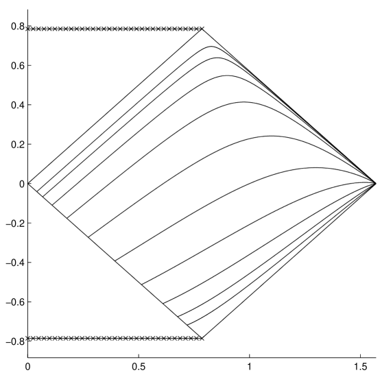
FIG. 2.: Penrose diagram for the exterior region of the Schwarzschild geometry.

The figure depicts the $t={\rm constant}$ slices for the time coordinate (172) in the exterior region of the Schwarzschild geometry. For the full construction and interpretation of the relevant Penrose diagram, see Ref. [61]. Here we define null coordinates (see Ref. [54], page 832)

$$\tilde{u} = -(R/2M-1)^{1/2}e^{R/4M}e^{-T/4M}$$ ()

$$\tilde{v} = (R/2M-1)^{1/2}e^{R/4M}e^{T/4M}\,,$$ ()

where our $\tilde{u}$ and $\tilde{v}$ correspond respectively to $w^{\prime}(2M)^{-1/2}$ and $v^{\prime}(2M)^{-1/2}$ of Ref. [61], page 153. Moreover, in Eqs. (() ‣ V Ca,b) the curvature coordinate $T=T(t,R)$, as determined by Eq. (172). Then the vertical and horizontal coordinates in the figure are defined as

$$\tau = {\textstyle\frac{1}{2}}\left[\tan^{-1}(\tilde{u})+\tan^{-1}(\tilde{v})\right]$$ ()

$$\rho = {\textstyle\frac{1}{2}}\left[\tan^{-1}(\tilde{u})-\tan^{-1}(\tilde{v})\right]\,.$$ ()

Starting from the bottom of the diagram, we have drawn level-time slices corresponding to $t=-6M,-4M,-2M,0M,2M,4M,6M,8M,10M,12M$. While the coordinate $t$ provides a good foliation of the shown exterior region, we note that these slices cross in the past dynamical region.

Now, with Eqs. (() ‣ V C) and (84) we find $K^{\theta}_{\theta}=K^{\phi}_{\phi}=-M/R^{2}$ for the components of $K_{ij}$ needed to compute $\ell=-8\pi\jmath_{\vdash}$, defined before in Eq. (() ‣ III Aa). Hence, with these components and with Eqs. (165) and (() ‣ V Cb) we obtain

$$8\pi\varepsilon = \frac{2M}{R^{2}}$$ ()

$$8\pi\jmath_{\vdash} = \frac{2M}{R^{2}}\,,$$ ()

again with $\kappa=8\pi$. It follows that both the total qle (161) and the total normal momentum $J_{\vdash}$, the proper surface integral of $\jmath_{\vdash}$, both have value $M$ for a sphere of any radius $R$ embedded in one of the hypersurfaces depicted in Fig. 2.

Now introduce a system boundary ${\bar{\cal T}}$ in the Schwarzschild exterior region determined by fixation of the areal radius $R=$ const, in which case the level-$t$ spacelike slices will not meet ${\bar{\cal T}}$ orthogonally. Observers at rest in the $t$ slices would see a changing areal radius $R$, because with the $t$-foliation normal $u$ considered as an operator $u[R]\neq 0$. We can compute the (referenced) quasilocal energy surface density $\bar{\varepsilon}$ for observers comoving with ${\bar{\cal T}}$. Although the energy density in Eq. (165) was not barred, we may nevertheless use that equation along with $r=R$ and $H=F^{1/2}$ to find

$$\bar{\varepsilon}=\frac{1}{4\pi R}\left(1-\sqrt{1-\frac{2M}{R}}\right)\,,$$ (177)

the result for a radius-$R$ round sphere embedded in a level-$T$ static slice. Upon proper integration over $B$, Eq. (177) gives Eq. (169) (although here we would denote the qle by $\bar{E}$). Note that because we have used $-2/R$ both for the implicit $k^{0}$ in Eq. (() ‣ V Ca) and for the implicit $\bar{k}{}^{0}$ in Eq. (177), the boost relations (() ‣ III B) are no longer valid (see the discussion in Sec. V.A pertaining to boosting reference terms). However, the point of this analysis –that our qle (and for that matter our quasilocal momentum) is inherently observer dependent– should be clear. There is in no strict sense one quasilocal energy expression for Schwarzschild.

D Isotropic Cosmology

Consider the standard isotropic cosmological model with line element

$$ds^{2}=-dt^{2}+a^{2}(t)[dr^{2}+f^{2}(r)(d\theta^{2}+\sin^{2}\theta d\phi^{2})]\,.$$ (178)

Here, $f(r)=\sin r$, $r$, or $\sinh r$ depending on whether space has positive ($\chi=+1$), zero ($\chi=0$), or negative ($\chi=-1$) curvature, respectively. The quasilocal energy within a sphere of coordinate radius $r$, embedded in a homogeneous surface $t={\rm const}$, can be obtained from the general result (166) for spherically symmetric spacetimes. Here, we compute the quasilocal energy within a sphere of fixed proper area $4\pi R^{2}$ (fixed areal radius $R$). That is, the history ${\bar{\cal T}}$ of the boundary $B$ is the surface $a(t)\,f(r)=R$, and the embedding hypersurface is chosen to be orthogonal to ${\bar{\cal T}}$. In the notation of Sec. II, we are computing the quasilocal energy density $\bar{\varepsilon}$ as seen by the (barred) observers who are comoving with the system boundary $a(t)\,f(r)=R$. In the calculation below we omit the bars.

The normal and tangent to the boundary $a(t)\,f(r)=R$ are given by

$$n^{\mu} = (-\alpha f{\dot{a}},\ \alpha f^{\prime}/a,\ 0,\ 0)\,,$$ ()

$$u^{\mu} = (\alpha f^{\prime},\ -\alpha f{\dot{a}}/a,\ 0,\ 0)\,,$$ ()

where $f^{\prime}=df/dr$, ${\dot{a}}=da/dt$, and $\alpha\equiv(f^{\prime}{}^{2}-f^{2}{\dot{a}}^{2})^{-1/2}$. We note that, with the definition for $f(r)$, $\alpha$ becomes

$$\alpha=\left(1-R^{2}(\chi+{\dot{a}}^{2})/a^{2}\right)^{-1/2}\,.$$ (180)

The mean curvature of the sphere is straightforward to compute, with the result

$$k=-\sigma^{\mu\nu}\nabla_{\mu}n_{\nu}=-\frac{2}{\alpha R}\,.$$ (181)

Combining this with the flat-space subtraction term $k^{0}=-2/R$, we find

$$E=8\pi R\left(1-\sqrt{1-R^{2}(\chi+{\dot{a}}^{2})/a^{2}}\right)\,$$ (182)

for the quasilocal energy.

The result above can be written in a more suggestive form by invoking the Einstein equation $(\chi+{\dot{a}}^{2})/a^{2}=8\pi\rho/3$, where $\rho$ is the proper energy density of matter including a contribution $\Lambda/8\pi$ from the cosmological constant. The quasilocal energy then becomes

$$E=8\pi R\left(1-\sqrt{1-8\pi\rho R^{2}/3}\right)\,.$$ (183)

This result for quasilocal energy has the same form as that given in Eqs. (168,169) for a static spherically symmetric solution, provided $M=0$ and $\rho={\rm const}$ in the definition (168) for $m(r)$. Note, however, that the matter energy density $\rho$ is constant on the homogeneous slices $t={\rm const}$, but is not constant on the hypersurfaces orthogonal to the system boundary $a(t)\,f(r)=R$.

E Cylindrical Waves

Finally, we turn to a non-spherically symmetric example, namely Einstein-Rosen cylindrical waves (see Ref. [62] and references therein) determined by a line-element of the following form:

$$ds^{2}=e^{\Gamma-\Phi}(-dt^{2}+dr^{2})+e^{-\Phi}r^{2}d\theta^{2}+e^{\Phi}dz^{2}\,,$$ (184)

where the coordinates $(t,r,\theta,z)$ range over their usual values. For the line-element (184) the vacuum Einstein equations become[62]

$$\partial^{2}_{t}\Phi-\partial^{2}_{r}\Phi-r^{-1}\partial_{r}\Phi=0\,,$$ (185)

where the function $\Gamma$ is written in terms of the scalar field $\Phi$ as

$$\Gamma(r,t)=\frac{1}{2}\int_{0}^{r}d\rho\,\rho\left[(\partial_{t}\Phi)^{2}+(\partial_{\rho}\Phi)^{2}\right]\,.$$ (186)

We assume smoothness at the origin, so that $\partial_{r}\Phi\rightarrow 0$ as $r\rightarrow 0$.

Ashtekar and Varadarajan, among others, have examined the $3+1$ vacuum Einstein equations under the assumption of a spacelike Killing vector field.[63] They show via “Killing vector field reduction” that the system is equivalent to the $2+1$ Einstein equations coupled to “fictitious” matter. Computing the total energy of the $2+1$ system, they thereby obtain a $3+1$ formula for energy per unit length along the Killing direction. The class of Einstein-Rosen cylindrical waves determined by the line-element (184) above –with two hypersurface orthogonal Killing vector fields– constitute a special case of their analysis. In this particular case, it is $\Phi$ which plays the role of matter from the $2+1$ viewpoint, and the expression they offer,

$$E_{\rm AV}=\frac{1}{4}\left(1-e^{-4C}\right)\,,$$ (187)

is for unit-length energy along the $\partial/\partial z$ direction. The $C$ in their expression is Thorne’s so-called $C$-energy[64], essentially just the total “flat-space energy” of the $\Phi$ scalar field,

$$C=\frac{1}{16}\int^{\infty}_{0}dr\,r\left[(\partial_{t}\Phi)^{2}+(\partial_{r}\Phi)^{2}\right]\,.$$ (188)

$E_{\rm AV}$ can be obtained directly from the integral (161). Consider an infinitely long cylindrical two-surface $B$ determined by fixation of $r$ and $t$. $B$ is embedded in a $\Sigma$ hypersurface determined by fixation of $t$. Let us compute the total qle (161) for a section of the cylinder of unit proper length in the $z$-direction. The mean curvature of the cylinder reads

$$k=-\frac{e^{(\Phi-\Gamma)/2}}{r}\,.$$ (189)

Now turn to the computation of the $k^{0}$ term. The $B$ metric functions are easily read off from the $B$ line-element,

$$ds^{2}=e^{\Phi}dz^{2}+e^{-\Phi}r^{2}d\theta^{2}\,.$$ (190)

Note that over the two-surface $B$ the field $\Phi$ is a constant, and from this we easily infer that for the auxiliary embedding of $B$ in ${\mathsf{E}}^{3}$ the associated mean curvature of the cylinder side is

$$k^{0}=-\frac{e^{\Phi/2}}{r}\,.$$ (191)

Hence, the energy (per unit proper length along the Killing direction $\partial/\partial z$) obtained from (161) is

$$E=\frac{1}{4}\left(1-e^{-\Gamma/2}\right)\,.$$ (192)

Comparing the definition (186) of $\Gamma(r,t)$ with the $C$-energy (188), we immediately see that the energy per unit proper length (192) agrees with the Ashtekar-Varadarajan expression (187) in the $r\rightarrow\infty$ limit.

VI Energy-momentum at spatial infinity

In this section we consider the quasilocal energy as applied to spacetimes that are asymptotically flat in spacelike directions[27, 65, 66, 67],¹⁵ and discuss its relationship with the standard treatment of energy at spatial infinity (spi). We begin by recalling the key observation from Regge and Teitelboim,[65] namely, that for asymptotically flat spacetimes the gravitational Hamiltonian must have well defined functional derivatives and must preserve the boundary conditions on the fields. This observation leads to a two step prescription for building the gravitational Hamiltonian. (i) Starting with the “base” Hamiltonian (93) (the smeared Hamiltonian and momentum constraints), one adds boundary terms and imposes boundary conditions so that the resulting Hamiltonian has well defined functional derivatives. For the Hamiltonian to have well defined functional derivatives the boundary terms in the variation of the Hamiltonian must vanish under the assumed boundary conditions. (ii) One checks that the boundary conditions are preserved under evolution by the Hamiltonian. If they are not, then the boundary conditions and boundary terms must be modified.

In essence, the canonical quasilocal formalism is an application of step (i) above to a manifold with boundary. That is, by working with the action in Hamiltonian form, we identify the appropriate boundary terms and boundary conditions that yield a Hamiltonian with well defined functional derivatives. The key difference between the quasilocal analysis and the asymptotically flat analysis is that in the quasilocal case we do not require, as in step (ii), that the Hamiltonian should preserve the boundary conditions. The reason is the following. In the asymptotically flat case the spacelike hypersurfaces $\Sigma$ are Cauchy surfaces. Thus, the data on one slice $\Sigma$ completely determines the future evolution of the system. For consistency the evolved data must obey the boundary conditions, otherwise the Hamiltonian on future $\Sigma$ slices will not have well defined functional derivatives. On the other hand, in the quasilocal context, the surfaces $\Sigma$ are not Cauchy surfaces. They do not carry enough information to determine the future evolution of the system (the spacetime interior to $\partial{\cal M}$). Therefore, we see that in the quasilocal case step (ii) cannot, and should not, be taken.

Note that the boundary conditions for our quasilocal Hamiltonian (124) and for the Regge-Teitelboim Hamiltonian for asymptotically flat spacetimes[65] both include fixation of the boundary two-metric, lapse function, and shift vector. In the asymptotically flat case, the boundary is at spi and the boundary values are determined through the specified asymptotic behaviors of the spatial metric, lapse, and shift. Although the boundary conditions for the two Hamiltonians are not specified in the same manner, they are at least “compatible” with one another. Also note that with the choice of flat space subtraction, the quasilocal energy (obtained from our quasilocal Hamiltonian with $N=1$ and $V^{i}=0$ on the boundary) vanishes for flat spacetime. Likewise, the ADM energy (obtained from the Regge-Teitelboim Hamiltonian with $N\to 1$ and $V^{i}\to 0$ at infinity) vanishes for flat spacetime.

To summarize, the quasilocal Hamiltonian and the Regge-Teitelboim Hamiltonian are both constructed from the base Hamiltonian by adding boundary terms and imposing “compatible” boundary conditions, so that their functional derivatives are well defined. Furthermore, in both cases, the energy obtained from these Hamiltonians is referenced to zero for flat spacetime. Given this close correspondence between the quasilocal and asymptotically flat analyses, it is not at all surprising that for asymptotically flat spacetimes the quasilocal energy agrees with the ADM energy in the limit that the spatial boundary $B$ is pushed to infinity. Although this result is not surprising, we find that a careful demonstration is nevertheless interesting and enlightening.¹⁶ The remainder of this section is devoted to this demonstration.

A Asymptotic flatness

For spacetimes that are asymptotically flat towards spi, the $\Sigma$ gravitational initial-data set $(h_{ij},K^{ij})$ obeys the following fall-off conditions:

$$h_{ij} = f_{ij}+\alpha_{ij}$$ ()

$$K^{ij} = O(r^{-2})\,.$$ ()

Here $f_{ij}$ is a flat background three-metric and $\alpha_{ij}$ an $O(r^{-1})$ perturbation thereof. The radial coordinate $r\equiv(f_{ij}x^{i}x^{j})^{1/2}$ is defined in terms of coordinates $x^{k}$ that are Cartesian with respect to the $f_{ij}$ metric. In this section we assume that the two-surface $B$ is a level-$r$ surface, that is to say a round sphere in the $f_{ij}$ metric (although not quite round in $h_{ij}$). The scalar curvature of $B$ then obeys

$${\cal R}=2r^{-2}+{}^{3}{\cal R}r^{-3}+O(r^{-3-\epsilon})$$ (194)

($\epsilon$ small and positive). We demand that $r$ is large enough such that ${\cal R}>0$ everywhere on $B$ (see comments near the end of Sec. V.A pertaining to Weyl’s problem). Adopting the usual distinction between “little-oh” and “big-oh” notation, we could write $o(r^{-3})$ instead of $O(r^{-3-\epsilon})$. The point being that $o(r^{-3})$ means “decay faster than $r^{-3}$ order” in this context. We call such a two-surface a large sphere.

B Momentum at spi

Momentum is identified with the phase space generator that moves the fields along the orbits of a spatial vector field $\xi^{i}$. In moving the fields along $\xi^{i}$, the changes in the fields at a given point are given by minus the Lie derivative along $\xi^{i}$. Thus, the quasilocal momentum in the $\xi^{i}$ direction is defined as the on-shell value of the Hamiltonian (124) with vanishing lapse $N=0$ and shift vector given by $V^{i}=-\xi^{i}$:

$$P_{\xi}\equiv H[0,-\xi]=\int_{B}d^{2}x\sqrt{\sigma}\,\xi^{i}\jmath_{i}\,.$$ (195)

Here, $\jmath_{i}=-2n^{k}P_{ki}/\sqrt{h}$ is the quasilocal momentum density (107). As discussed in Sec. V.A, with Euclidean reference there is no reference contribution to $\jmath_{i}$, because as it stands $\jmath_{i}$ would already vanish were $\Sigma$ an inertial ${\mathsf{E}}^{3}$ hyperplane of Minkowski spacetime. In other words, the reference contribution $-2(n^{k}P_{ki}/\sqrt{h})|^{0}$ to $\jmath_{i}$ vanishes for the Euclidean subtraction at hand. This is so because an inertial hyperplane of Minkowski spacetime has a vanishing extrinsic curvature tensor. Now consider the case in which space is asymptotically flat, and the boundary $B$ is pushed to infinity. If the vector $\xi$ to chosen to be an asymptotic translation, then we immediately find that the momentum $P_{\xi}$ above agrees with the ADM momentum at infinity.[27, 65] If the vector $\xi$ is chosen to be an asymptotic rotation, then the momentum $P_{\xi}$ agrees with the angular momentum at infinity.[65] [Although here appearing in the context of asymptotic flatness, note that the integral (195) is the most general expression for quasilocal momentum in the $\xi^{i}$ direction, if we take $\jmath_{i}=-2n^{k}P_{ki}/\sqrt{h}+2(n^{k}P_{ki}/\sqrt{h})|^{0}$, now assuming that $-2(n^{k}P_{ki}/\sqrt{h})|^{0}$ need not arise from Euclideain reference and hence may be non-zero.]

C Energy at spi

Consider the quasilocal energy (161), now with $B$ a large sphere in the sense described above.¹⁷ Let us show the equivalence between the qle and the adm energy. Note that $B$ is a Riemannian submanifold of the Riemannian space $\Sigma$. Let us examine the geometry of this embedding in order to obtain an asymptotic expression for the integral (161) in terms of the $\Sigma$ Riemann tensor. Recall the Gauss-Codazzi-Mainardi constraints[51] which relate the intrinsic geometry $\sigma_{ab}$ (or $\cal R$) and extrinsic geometry $k_{ab}$ (of $B$ in $\Sigma$) to the $\Sigma$ Riemann tensor. Among these is the following:

$${\cal R}-k{}^{2}+k_{ab}k^{ab}=\sigma^{ik}\sigma^{jl}R_{ijkl}\,.$$ (196)

As the $\Sigma$ Riemann tensor is completely determined by the Ricci tensor $R_{ij}$ in three dimensions, we may replace the rhs of Eq. (196) with Ricci terms using the identity

$$\sigma^{ik}\sigma^{jl}R_{ijkl}=R-2R_{\vdash\vdash}\,,$$ (197)

where $\vdash$ denotes contraction with the $B$ normal $n^{k}$. Splitting $k_{ab}=:\frac{1}{2}k\sigma^{ab}+(k^{\rm TF})^{ab}$ into its trace and trace-free pieces, we rewrite Eq. (196) as

$${\cal R}-{\textstyle\frac{1}{2}}k{}^{2}+(k^{\rm TF})_{ab}(k^{\rm TF}){}^{ab}=\sigma^{ik}\sigma^{jl}R_{ijkl}\,.$$ (198)

From this equation we may easily obtain the relevant leading order asymptotic relationship between $k$ and the $\Sigma$ Riemann tensor. Now, the fall-off of the $\Sigma$ metric $h_{ij}$ determines that

$$\sigma^{ik}\sigma^{jl}R_{ijkl}={}^{3}(\sigma^{ik}\sigma^{jl}R_{ijkl})r^{-3}+o(r^{-3})\,,$$ (199)

with the superscript $3$ meaning take the $O(r^{-3})$ piece of that inside the parenthesis. Now we make the Ansätze¹⁸

$$k = -2r^{-1}+{}^{2}kr^{-2}+o(r^{-2})$$ ()

$$(k^{\rm TF})_{ab} = O(r^{-2})$$ ()

Using the Ansätze (() ‣ VI C) along with the expansion (194) in Eq. (198), we quickly find

$${}^{2}k={\textstyle\frac{1}{2}}\,{}^{3}(\sigma^{ik}\sigma^{jl}R_{ijkl}-{\cal R})\,.$$ (201)

Along a similar line, we can compute the asymptotic form of $k^{0}$, also appearing in Eq. (161). Indeed, striking the Riemann curvature term from the rhs of Eq. (198) and replacing all $k$’s with $k^{0}$’s, we get a valid constraint for the auxiliary embedding of $B$ in ${\mathsf{E}}^{3}$ [see Eq. (() ‣ V Aa)]. An asymptotic analysis of the resulting equations shows that

$${}^{2}k^{0}=-{\textstyle\frac{1}{2}}\,{}^{3}{\cal R}\,.$$ (202)

It follows that the quasilocal energy surface density $\varepsilon=(k-k^{0})/(8\pi)$ obeys

$$8\pi\varepsilon={\textstyle\frac{1}{2}}\,{}^{3}(\sigma^{ik}\sigma^{jl}R_{ijkl})+o(r^{-2})$$ (203)

in the asymptotic setting described here.

Eq. (203) shows that the spi definition of energy determined by the canonical quasilocal energy (161) is equivalent to the (rather symbolic) integral

$$E_{\infty}=\frac{1}{16\pi}\oint_{\infty}d^{2}x\sqrt{\sigma}\,r\sigma^{ik}\sigma^{jl}R_{ijkl},$$ (204)

where we use $\oint_{\infty}$ as shorthand for $\lim_{r\rightarrow\infty}\int_{B}$ so that $\sqrt{\sigma}$ tends to $r^{2}\sin\theta$. We can rewrite this integral in a familiar form. Recall that $\Re_{ijkl}=R_{ijkl}\,+$ terms quadratic in the extrinsic tensor $K_{ij}$ [and hence $O(r^{-4})$ terms], where $\Re_{ijkl}$ is the $\Sigma$ projection of the spacetime Riemann tensor $\Re_{\mu\nu\lambda\kappa}$ (the same as the Weyl tensor $C_{\mu\nu\lambda\kappa}$ near spi). Moreover, we may use $r\sim\sqrt{A/(4\pi)}$ where $A$ is the area of $B$. Therefore, the integral above agrees asymptotically with what Hayward[59] calls the Ashtekar-Hansen expression¹⁹

$$E_{\rm AH}=\frac{1}{8\pi}\sqrt{\frac{A}{16\pi}}\int_{B}d^{2}x\sqrt{\sigma}\,\sigma^{\mu\lambda}\sigma^{\nu\kappa}C_{\mu\nu\lambda\kappa}\,,$$ (205)

which is quite similar to Hayward’s mass Eq. (73). The Ashtekar-Hasen expression agrees asymptotically with

$$E_{\rm ADM}=\frac{1}{16\pi}\oint_{\infty}d^{2}x\sqrt{\sigma}\,n^{k}\left(\partial^{j}\alpha_{kj}-\partial_{k}\alpha^{j}{}_{j}\right)\,,$$ (206)

the familiar adm energy. We can replace $\sqrt{\sigma}\,n^{k}$ with $rx^{k}\sin\theta$ in this integral.

Although apparently a result known for some time[71], let us briefly argue why the integrals (204) and (206) agree in the spi limit considered here. A more detail account of this issue and others concerning surface integrals at spi will appear elsewhere.[72] First, replace the Riemann curvature term in the integral (204) in favor of Ricci terms using the identity (197). Next, via standard techniques, obtain the identity

$${}^{3}\!R_{ij}={}^{3}\!\left[\partial^{p}\partial_{(i}\alpha_{j)p}-{\textstyle\frac{1}{2}}\partial^{k}\partial_{k}\alpha_{ij}-{\textstyle\frac{1}{2}}\partial_{i}\partial_{j}\alpha^{p}{}_{p}\right]\,,$$ (207)

where the $\partial_{k}$’s are Cartesian partial derivatives. Note that one is taking the $O(r^{-3})$ piece of the rhs of the above equation. Finally, use this last identity along with the useful fact that $\partial_{r}\alpha_{ij}=-r^{-1}\alpha_{ij}+o(r^{-2})$, to show that –at leading order– the integrands in (204) and (206) differ by a pure divergence on the unit sphere.

VII Acknowledgments

This work was conducted over a eight year period of time, beginning in 1993. During this time, SRL visited the Raman Research Institute on two separate occasions, and he doubly thanks that institute, and in particular J. Samuel, for hospitality. JDB would like to thank the Department of Mathematics, North Carolina State University, for support during the early stages of this work. We also thank both J. Jezierski for discussions and for bringing Ref. [52] to our attention and A. N. Petrov for several email communications on the topic of energy at spatial infinity. This work was supported in part by National Science Foundation grants PHY-0070892 to North Carolina State University, and PHY-9972582 to the University of North Carolina.

Note Added: Recently, Anco and Tung have also carried out a careful systematic analysis of gravitational boundary conditions for a quasilocal spacetime region, one based on a general Noether charge formulation.[25]

A Kinematics of a double foliation

Consider a double foliation of spacetime into $t={\rm const}$ surfaces and $s={\rm const}$ surfaces, where $t={\rm const}$ is spacelike with leaves $\Sigma$ and $s={\rm const}$ is timelike with one of its leaves ${\bar{\cal T}}$. Let

$$u_{\mu} = -N\nabla_{\mu}t\ ,$$ ()

$${\bar{n}}_{\mu} = {\bar{M}}\nabla_{\mu}s\ ,$$ ()

denote the unit-normal covectors of the $t={\rm const}$ and $s={\rm const}$ surfaces, respectively. Note that $N$ and ${\bar{M}}$ serve to normalize these vectors, so $u\cdot u=-1$ and ${\bar{n}}\cdot{\bar{n}}=+1$. The induced (projection) metrics for the $t$ and $s$ foliations are

$$h_{\mu\nu} = g_{\mu\nu}+u_{\mu}u_{\nu}\ ,$$ ()

$${\bar{\gamma}}_{\mu\nu} = g_{\mu\nu}-{\bar{n}}_{\mu}{\bar{n}}_{\nu}\ ,$$ ()

respectively. Also define the new unit vector fields

$$n_{\mu} = MD_{\mu}s=Mh_{\mu}^{\nu}\nabla_{\nu}s=(M/{\bar{M}})h_{\mu}^{\nu}{\bar{n}}_{\nu}\ ,$$ ()

$${\bar{u}}_{\mu} = -{\bar{N}}{\cal D}_{\mu}t=-{\bar{N}}{\bar{\gamma}}_{\mu}^{\nu}\nabla_{\nu}t=({\bar{N}}/N){\bar{\gamma}}_{\mu}^{\nu}u_{\nu}\ ,$$ ()

where $D_{\mu}$ is the covariant derivative on $t={\rm const}$, and ${\cal D}_{\mu}$ is the covariant derivative on $s={\rm const}$. $M$ and ${\bar{N}}$ are chosen so that $n\cdot n=+1$ and ${\bar{u}}\cdot{\bar{u}}=-1$. The covectors $n_{\mu}$, ${\bar{u}}_{\mu}$ lie in the $t={\rm const}$, $s={\rm const}$ surfaces, respectively, and are orthogonal to the two–surfaces formed by the intersections of the double foliation. In general $n_{\mu}$ and ${\bar{u}}_{\mu}$ are not three–surface orthogonal. For example, whereas ${\bar{u}}^{\mu}$ is indeed two–surface orthogonal as a vector field within a single $s={\rm const}$ three–surface (as the future–pointing normal to the $B$ foliation), ${\bar{u}}^{\mu}$ need not define a foliation of ${\cal M}$ into spacelike three–surfaces. The spacetime representation of the $B$ two–metric may now be expressed in two ways:

$$\sigma_{\mu\nu}=g_{\mu\nu}+u_{\mu}u_{\nu}-n_{\mu}n_{\nu}=g_{\mu\nu}+{\bar{u}}_{\mu}{\bar{u}}_{\nu}-{\bar{n}}_{\mu}{\bar{n}}_{\nu}{\,}.$$ (A4)

Now define a time flow vector field $t^{\mu}$ along the $s={\rm const}$ surfaces by the conditions

$$t^{\mu}\nabla_{\mu}t=1\ ,\qquad t^{\mu}\nabla_{\mu}s=0\ .$$ (A5)

Likewise, fix a space flow vector field $s^{\mu}$ along the $t={\rm const}$ surfaces by the conditions

$$s^{\mu}\nabla_{\mu}s=1\ ,\qquad s^{\mu}\nabla_{\mu}t=0\ .$$ (A6)

Then the shift vectors for the double foliation are given by

$$V^{\mu} = h^{\mu}_{\nu}t^{\nu}\ ,$$ ()

$${\bar{W}}^{\mu} = {\bar{\gamma}}^{\mu}_{\nu}s^{\nu}\ .$$ ()

The time and space flow vector fields can also be written as

$$t^{\mu} = Nu^{\mu}+V^{\mu}\ ,$$ ()

$$s^{\mu} = {\bar{M}}{\bar{n}}^{\mu}+{\bar{W}}^{\mu}\ ,$$ ()

respectively.

Using the expressions (() ‣ Ab) for the normal ${\bar{n}}_{\mu}$ and (() ‣ Aa) for the time flow vector field $t^{\mu}$, we find that $u^{\mu}{\bar{n}}_{\mu}=({\bar{M}}/N)(t^{\mu}-V^{\mu})\nabla_{\mu}s=-({\bar{M}}/M)v$, where the proper “radial” velocity is defined by $v=V\cdot n/N$. In deriving this result, Eqs. (() ‣ Aa) and (A5a) were used. A similar calculation using the expressions (() ‣ Aa) and (() ‣ Ab) for the normal $u_{\mu}$ and the space flow vector field $s^{\mu}$ yields ${\bar{n}}^{\mu}u_{\mu}=-(N/{\bar{M}})(s^{\mu}-{\bar{W}}^{\mu})\nabla_{\mu}t=-(N/{\bar{N}})({\bar{W}}\cdot{\bar{u}}/{\bar{M}})$. Putting these results together, we have (using a “$\cdot$” to denote spacetime inner product)

$$u\cdot{\bar{n}}=-\frac{{\bar{M}}}{M}v=-\frac{N}{{\bar{N}}}\left(\frac{{\bar{W}}\cdot{\bar{u}}}{{\bar{M}}}\right)\ .$$ (A10)

The normalization condition for $n_{\mu}$ implies

$$M = (D_{\mu}s\,g^{\mu\nu}\,D_{\nu}s)^{-1/2}=(\nabla_{\mu}s\,h^{\mu\nu}\,\nabla_{\nu}s)^{-1/2}$$ (A11)

$$= {\bar{M}}({\bar{n}}_{\mu}h^{\mu\nu}{\bar{n}}_{\nu})^{-1/2}={\bar{M}}(1+(u\cdot{\bar{n}})^{2})^{-1/2}$$ (A12)

$$= {\bar{M}}(1+({\bar{M}}v/M)^{2})^{-1/2}\ .$$ (A13)

Solving for $M$, we find $M={\bar{M}}/\gamma$ where $\gamma=(1-v^{2})^{-1/2}$. This implies, from Eq. (A10), that $u\cdot{\bar{n}}=-\gamma v$. A calculation similar to the one in Eq. (A13) for the normalization condition on ${\bar{u}}_{\mu}$ gives ${\bar{N}}=N/\gamma$. Now Eq. (A10) shows that $({\bar{W}}\cdot{\bar{u}}/{\bar{M}})=v$. To summarize the results thus far, we have

$$v = \frac{V\cdot n}{N}=\frac{{\bar{W}}\cdot{\bar{u}}}{{\bar{M}}}\ ,$$ ()

$$\gamma = \frac{N}{{\bar{N}}}=\frac{{\bar{M}}}{M}\ ,$$ ()

where $\gamma=(1-v^{2})^{-1/2}$.

Our next task is to express the barred unit vectors in terms of the unbarred unit vectors. From the definition (() ‣ Ab) of ${\bar{u}}_{\mu}$, we have

$${\bar{u}}_{\mu} = ({\bar{N}}/N){\bar{\gamma}}_{\mu}^{\nu}u_{\nu}$$ (A15)

$$= ({\bar{N}}/N)(u_{\mu}-(u\cdot{\bar{n}}){\bar{n}}_{\mu})$$ (A16)

$$= (1/\gamma)(u_{\mu}+\gamma v{\bar{n}}_{\mu})\ ,$$ (A17)

with a similar calculation showing that

$$n_{\mu}=(1/\gamma)({\bar{n}}_{\mu}-\gamma vu_{\mu})\ .$$ (A18)

Putting these together, we find

$${\bar{n}}_{\mu} = \gamma n_{\mu}+\gamma vu_{\mu}\ ,$$ ()

$${\bar{u}}_{\mu} = \gamma u_{\mu}+\gamma vn_{\mu}\ .$$ ()

Equivalently, we obtain

$$n_{\mu} = \gamma{\bar{n}}_{\mu}-\gamma v{\bar{u}}_{\mu}\ ,$$ ()

$$u_{\mu} = \gamma{\bar{u}}_{\mu}-\gamma v{\bar{n}}_{\mu}\ ,$$ ()

by inverting Eqs. (() ‣ A).

We now derive two useful expressions, one for ${\bar{u}}^{\mu}$ in terms of $t^{\mu}$ and the other for $n^{\mu}$ in terms of $s^{\mu}$. Begin with the definition (() ‣ Aa) for the time flow vector field $t^{\mu}$ and write the shift vector as $V^{\mu}=h^{\mu}_{\nu}V^{\nu}=\sigma^{\mu}_{\nu}V^{\nu}+N^{\mu}(V\cdot n)$. Using the formulas (() ‣ A) and (() ‣ Ia) we find

$${\bar{N}}{\bar{u}}^{\mu}=t^{\mu}-\sigma^{\mu}_{\nu}V^{\nu}\ .$$ (A21)

A similar calculation starting from the definition (() ‣ Ab) for the space flow vector field $s^{\mu}$ yields

$$Mn^{\mu}=s^{\mu}-\sigma^{\mu}_{\nu}{\bar{W}}^{\nu}\ ,$$ (A22)

where equations (() ‣ A) and (() ‣ Aa) are used.

The foliation of spacetime into $t={\rm const}$ surfaces is pictured in Fig. 3.

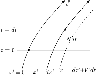
FIG. 3.:

The proper time between $t={\rm const}$ slices, measured orthogonal to the slices, is $N\,dt$. In the diagram the shift vector $V^{\mu}$ points to the right, along the direction of increasing $x^{i}$, so the component $V^{i}$ is positive. The proper distance between the heavy dots is

$$ds^{2}=-N^{2}dt^{2}+h_{ij}(dx^{i}+V^{i}dt)(dx^{j}+V^{j}dt)\ ,$$ (A23)

where $h_{ij}$ is the metric on $t={\rm const}$.

The foliation of spacetime into $s={\rm const}$ surfaces is pictured in Fig. 4.

FIG. 4.:

The proper distance between $s={\rm const}$ slices, measured orthogonal to the slices, is ${\bar{M}}\,ds$. In the diagram the shift vector ${\bar{W}}^{\mu}$ points to the past, along the direction of decreasing $x^{i}$, so the component ${\bar{W}}^{i}$ is negative. The proper distance between the heavy dots is

$$ds^{2}={\bar{M}}^{2}ds^{2}+{\bar{\gamma}}_{ij}(dx^{i}+{\bar{W}}^{i}ds)(dx^{j}+{\bar{W}}^{j}ds)\ ,$$ (A24)

where ${\bar{\gamma}}_{ij}$ is the metric on $s={\rm const}$.

B Extrinsic Curvature “splittings”

Let us now derive the splitting expression (44) as well as easier splitting (52) for $K_{ij}$. Recall that the ${\bar{\cal T}}$ extrinsic curvature is defined by ${\bar{\Theta}}_{\mu\nu}\equiv-{\bar{\gamma}}^{\alpha}_{\mu}\nabla_{\alpha}{\bar{n}}_{\nu}$. With the identity

$$\nabla_{\mu}u_{\nu}=-K_{\mu\nu}-u_{\mu}a_{\nu}\ ,$$ (B1)

and the definitions $v\gamma=-u\cdot{\bar{n}}$ and $\gamma=(1-v^{2})^{-1/2}$, it is straightforward to verify that

$$\nabla_{\mu}{\bar{n}}_{\nu}=\gamma\,\nabla_{\mu}n_{\nu}-\gamma v\,K_{\mu\nu}-\gamma v\,u_{\mu}a_{\nu}+\gamma^{2}\,{\bar{u}}_{\nu}\,\nabla_{\mu}v\ .$$ (B2)

From this result it follows that the projection of ${\bar{\Theta}}_{\mu\nu}$ into $B$ is $\sigma^{\alpha}_{\mu}\sigma^{\beta}_{\nu}{\bar{\Theta}}_{\alpha\beta}=\gamma k_{\mu\nu}+\gamma v\sigma^{\alpha}_{\mu}\sigma^{\beta}_{\nu}K_{\alpha\beta}$, where $k_{\mu\nu}=-\sigma^{\alpha}_{\mu}D_{\alpha}n_{\nu}$ is the extrinsic curvature of $B$ embedded in $t={\rm const}$. The identity (B1) and the definition (() ‣ III Ab) show that the term $\sigma^{\alpha}_{\mu}\sigma^{\beta}_{\nu}K_{\alpha\beta}$ equals the extrinsic curvature $\ell_{\mu\nu}$ of $B$ embedded in a surface whose normal at $B$ coincides with $n^{\mu}$. Thus, we find

$$\sigma^{\alpha}_{\mu}\sigma^{\beta}_{\nu}{\bar{\Theta}}_{\alpha\beta}=\gamma k_{\mu\nu}+\gamma v\ell_{\mu\nu}\ .$$ (B3)

Next, we note that

$${\bar{u}}^{\mu}{\bar{u}}^{\nu}{\bar{\Theta}}_{\mu\nu} = -{\bar{u}}^{\mu}{\bar{u}}^{\nu}\nabla_{\mu}{\bar{n}}_{\nu}$$ (B4)

$$= {\bar{n}}\cdot{\bar{a}}\ ,$$ (B5)

where we have used the Leibniz rule ${\bar{u}}^{\nu}\nabla_{\mu}{\bar{n}}_{\nu}=\nabla_{\mu}({\bar{u}}^{\nu}{\bar{n}}_{\nu})-{\bar{n}}_{\nu}\nabla_{\mu}{\bar{u}}^{\nu}=-{\bar{n}}_{\nu}\nabla_{\mu}{\bar{u}}^{\nu}$ and the definition $a^{\nu}={\bar{u}}^{\mu}\nabla_{\mu}{\bar{u}}^{\nu}$ of the acceleration of ${\bar{u}}^{\nu}$. Finally, we compute

$$\sigma^{\alpha}_{\mu}{\bar{u}}^{\beta}{\bar{\Theta}}_{\alpha\beta} = -\sigma^{\alpha}_{\mu}{\bar{u}}^{\beta}\nabla_{\alpha}{\bar{n}}_{\beta}$$ (B6)

$$= -\sigma^{\alpha}_{\mu}{\bar{u}}^{\beta}\left(\gamma\,\nabla_{\alpha}n_{\beta}-\gamma v\,K_{\alpha\beta}-\gamma v\,u_{\alpha}a_{\beta}+\gamma^{2}\,{\bar{u}}_{\beta}\nabla_{\alpha}v\right)$$ (B7)

$$= -\gamma^{2}\,\sigma^{\alpha}_{\mu}u^{\beta}\nabla_{\alpha}n_{\beta}+\gamma^{2}v^{2}\sigma^{\alpha}_{\mu}n^{\beta}K_{\alpha\beta}+\gamma^{2}\,\sigma^{\alpha}_{\mu}\nabla_{\alpha}v\ ,$$ (B8)

where Eqs. (() ‣ Ia) and (B2) have been used. Application of the Leibniz rule on the first term on the right–hand side above yields $\sigma^{\alpha}_{\mu}u^{\beta}\nabla_{\alpha}n_{\beta}=-\sigma^{\alpha}_{\mu}n_{\beta}\nabla_{\alpha}u^{\beta}=\sigma^{\alpha}_{\mu}n^{\beta}K_{\alpha\beta}$. Collecting terms, we find

$$\sigma^{\alpha}_{\mu}{\bar{u}}^{\beta}{\bar{\Theta}}_{\alpha\beta}=-\sigma^{\alpha}_{\mu}n^{\beta}K_{\alpha\beta}+\gamma^{2}\sigma^{\alpha}_{\mu}\nabla_{\alpha}v\ .$$ (B9)

The results (B3), (B5), and (B9) then give Eq. (44).

The expression (44) for ${\bar{\Theta}}_{\mu\nu}$ still retains reference to barred quantities through the appearance of ${\bar{u}}^{\mu}$ and ${\bar{n}}\cdot{\bar{a}}$. Definitions (() ‣ I) can be used to eliminate ${\bar{u}}^{\mu}$ in favor of $u^{\mu}$ and $n^{\mu}$. The acceleration ${\bar{n}}\cdot{\bar{a}}$ can be re-expressed with the help of Eq. (B2):

$${\bar{n}}\cdot{\bar{a}} = {\bar{n}}_{\nu}{\bar{u}}^{\mu}\nabla_{\mu}{\bar{u}}^{\nu}$$ (B10)

$$= -{\bar{u}}^{\mu}{\bar{u}}^{\nu}\nabla_{\mu}{\bar{n}}_{\nu}$$ (B11)

$$= -{\bar{u}}^{\mu}{\bar{u}}^{\nu}\left(\gamma\nabla_{\mu}n_{\nu}-\gamma v\,K_{\mu\nu}-\gamma v\,u_{\mu}a_{\nu}+\gamma^{2}{\bar{u}}_{\nu}\,\nabla_{\mu}v\right)$$ (B12)

$$= -\gamma^{2}{\bar{u}}^{\mu}u^{\nu}\nabla_{\mu}n_{\nu}+\gamma^{3}v^{3}n^{\mu}n^{\nu}K_{\mu\nu}-\gamma^{3}v^{2}n\cdot a+\gamma^{2}{\bar{u}}^{\mu}\nabla_{\mu}v\ .$$ (B13)

The first term on the right–hand side of the last line can be re-expressed as

$${\bar{u}}^{\mu}\,u^{\nu}\nabla_{\mu}n_{\nu} = {\bar{u}}^{\mu}n^{\nu}\left(K_{\mu\nu}+u_{\mu}a_{\nu}\right)$$ (B14)

$$= \gamma v\,n^{\mu}n^{\nu}K_{\mu\nu}-\gamma\,n\cdot a\ ,$$ (B15)

which leads to

$${\bar{n}}\cdot{\bar{a}}=-\gamma v\,n^{\mu}n^{\nu}K_{\mu\nu}+\gamma\,n\cdot a+\gamma^{2}{\bar{u}}^{\mu}\nabla_{\mu}v\ .$$ (B16)

The extrinsic curvature term $n^{\mu}n^{\nu}K_{\mu\nu}$ can be rewritten using the identity (B1) followed by an integration by parts; this leads to $n^{\mu}n^{\nu}K_{\mu\nu}=u\cdot b$, where $b^{\mu}=n^{\nu}\nabla_{\nu}n^{\mu}$. Collecting results, we find

$${\bar{n}}\cdot{\bar{a}}=\gamma\,n\cdot a-\gamma v\,u\cdot b+{\bar{u}}\cdot\nabla\theta\ .$$ (B17)

This is Eq. (() ‣ III Ba) from the main text.

The derivation of the splitting (52) amounts to simply projecting $K_{ij}$ into various pieces normal and tangential to $B$. We leave this to the reader. Let us however sketch the derivation of Eq. (() ‣ III Bb). Using the boost relations (() ‣ I) and the identity (B1), we find

$$\nabla_{\alpha}{\bar{u}}_{\nu}=\gamma v\nabla_{\alpha}n_{\nu}-\gamma K_{\alpha\nu}-\gamma u_{\alpha}a_{\nu}+\gamma^{2}{\bar{n}}_{\nu}\nabla_{\alpha}v\ ,$$ (B18)

from which the quantity ${\bar{n}}\cdot{\bar{b}}=-{\bar{n}}^{\mu}{\bar{n}}^{\nu}\nabla_{\mu}{\bar{u}}_{\nu}$ can be expressed in terms of unbarred quantities [with result (() ‣ III Bb)].

C Velocity parameter $\theta$ and its time rate of change

Let us turn to the interpretation of $\dot{\theta}$ defined in Eq. (131). We have defined $\dot{\theta}$ as such in order that $\theta$ is the velocity parameter. We may verify the correctness of our assignment by considering boosts in flat spacetime. Let

$$T = x\sinh t\ ,$$ ()

$$X = x\cosh t\ ,$$ ()

where $X$, $T$ are Minkowski coordinates and $x$, $t$ are Rindler coordinates. See Fig. 5.

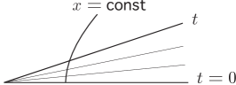
FIG. 5.:

The metric is $ds^{2}=-dT^{2}+dX^{2}=-x^{2}dt^{2}+dx^{2}$. The four–velocity $U(t)$ along $x={\rm const}$ at Rindler time $t$ is $U(t)=(1/x)(\partial/\partial t)=\cosh t(\partial/\partial T)+\sinh t(\partial/\partial X)$. The relativistic gamma factor between the four–velocities at $t=0$ and $t$ is²⁰ $\gamma=-U(t)\cdot U(0)=\cosh t$. Now let $\tau=xt$ denote the proper time along $x={\rm const}$ between $t=0$ and $t$. The rate of change of $\tau$ with respect to proper distance along $t={\rm const}$ is $d\tau/dx=t=\cosh^{-1}\gamma$. This also can be expressed in terms of the gradient of the lapse function: $d\tau/dx=\int_{0}^{t}(n^{i}\partial_{i}\eta)$ Thus, we find $\gamma=\cosh\int_{0}^{t}(n^{i}\partial_{i}\eta)dt$. From the definition of the velocity parameter, we have $\gamma=\cosh\theta$ so that

$$\theta(t)=\int_{0}^{t}(n^{i}\partial_{i}\eta)dt\,.$$ (C2)

It follows that $n^{i}\partial_{i}\eta={\dot{\theta}}$, from which we obtain Eq. (131). Ref. [26] discusses these results in terms of degenerate foliations.

FOOTNOTES

1. This is not an exhaustive list.

2. See also the related work [38] by Freud.

3. For a comparison of the Trace-K action with the tetrad action of Goldberg, see Ref. [12].

4. With the Trace-K action, as with any action, we are free to subtract a function of the fixed boundary data. In some cases, it is convenient to fix this ambiguity by introducing a background space or spacetime. However, this is not a required feature of the cqf. See Sec. V.A for further discussion.

5. Thus both $\Sigma^{\prime}$ and $\Sigma^{\prime\prime}$ are, as the notation suggests, leaves of the $\Sigma$ foliation. We have investigated the more general case in which $\Sigma^{\prime}$ and $\Sigma^{\prime\prime}$ are not leaves of $\Sigma$, in which case some portions of the boundaries of some $\Sigma$ leaves lie in the boundary elements $\Sigma^{\prime\prime}$ or $\Sigma^{\prime}$. However, at present we find no compelling reason to allow for such generality.

6. By introducing a partial foliation of ${\cal M}$ that includes ${\bar{\cal T}}$ as one leaf, we can define ${\bar{u}}^{\mu}$ and $n^{\mu}$ as unit vector fields in a spacetime neighborhood of ${\bar{\cal T}}$. Note, however, that as spacetime vector fields, ${\bar{u}}^{\mu}$ and $n^{\mu}$ are not in general hypersurface orthogonal. See Appendix A.

7. A few words concerning terminology are in order. When we apply the variational principle, we vary the action functional among all histories that satisfy certain specified boundary conditions. The histories that extremize the action under such a variation are, by definition, the classical histories. On the other hand, a Hamilton–Jacobi variation (hj variation) of the action is a variation among classical histories with different boundary values.

8. Or, indeed, useful when examining any variation involving a Ricci scalar curvature (we have in mind the Ricci–scalar term present in the initial–value Hamiltonian constraint).

9. For $u^{\mu}$, of course, $\epsilon=-1$, but we shall keep track of $\epsilon$ in order to ensure that the lemma also holds for $\bar{n}^{\mu}$.

10. However, the reader should resist the temptation to identify ${\bar{u}}^{\mu}$ with the future–pointing normal of ${\bar{\Sigma}}$, as in our formalism ${\bar{u}}^{\mu}$ need not be three–surface orthogonal. It is the case that the ${\bar{\Sigma}}$ normal agrees with ${\bar{u}}^{\mu}$ on the two–surface $B$ where ${\bar{\Sigma}}$ and ${\bar{\cal T}}$ intersect. In fact, this is all that we require of $\bar{\Sigma}$, so in effect ${\bar{\Sigma}}$ represents an equivalence class of three–slices determined by this condition on $B$.

11. In that paper, the bars were omitted.

12. The most effective way to proceed is to use the result for the variation of the Hamiltonian, derived below.

13. Nevertheless, let us present some details here. Typically, the subtraction term will arise as a sum of functionals (smearing integrals) over each boundary element,

$$-S^{0}[{\bar{\gamma}}_{ij},h_{ij}]=-S^{0}_{\bar{\cal T}}[{\bar{\gamma}}_{ij}]-S^{0}_{\Sigma^{\prime\prime}}[h_{ij}]+S^{0}_{\Sigma^{\prime}}[h_{ij}]\,,$$

where $S^{0}_{\Sigma^{\prime\prime}}$ and $S^{0}_{\Sigma^{\prime}}$ are the same functional. The $\Sigma^{\prime}$ and $\Sigma^{\prime\prime}$ contributions to $-S^{0}$ give rise to canonical transformation of the gravitational momentum $P^{ij}$ defined in Eq. (() ‣ IIa). The ${\bar{\cal T}}$ contribution modifies $\bar{\Pi}^{ij}$ in Eq. (() ‣ IIb). Modification of $\bar{\Pi}^{ij}$ corresponds to the zero–point freedom in $\bar{\varepsilon}$, ${\bar{\jmath}}_{a}$, and $\bar{s}{}^{ab}$.

14. See Ref. [9] for the origins of this transformation. It may also be found by carrying out the null limit construction described in Ref. [16] for the particular case of Schwarzschild.

15. A similar analysis can be carried out for spacetimes which are asymptotically anti-de Sitter[68]; and in particular, by inclusion of a lapse factor into the energy surface integral, one can recover the Abbott-Deser definition energy [69] in the $r\rightarrow\infty$ limit.[8, 14, 21]

16. The detailed connection between the quasilocal energy and the ADM energy has not been derived previously in the literature. See, however, Refs. [8, 14].

17. Be careful not to confuse the metric $f_{ij}$ with the Euclidean metric of the auxiliary space ${\mathsf{E}}^{3}$ used to obtain $k^{0}$, for the metric $f_{ij}$ lives on $\Sigma$.

18. These Ansätze can be confirmed directly by computing $k_{ab}$ in linear approximation, a calculation which uses the fall-off of $h_{ij}$ and the fact that $\partial_{k}r$ is proportional to the one-form normal $n_{k}$ of $B$ in $\Sigma$.

19. Ashtekar and Hansen[70] define an expression at infinity via a conformal compactification. This integral is the physical spacetime version of the Ashtekar-Hansen expression.

20. The four–velocity $U(t)$ is expressed in Minkowski coordinates so that its components are unchanged when $U(t)$ is parallel transported to $t=0$.

REFERENCES

- [1] J. D. Brown and J. W. York, Phys. Rev. D47, (1993) 1407.
- [2] G. Hayward and K. Wong, Phys. Rev. D46, (1992) 620; D47, (1993) 4778.
- [3] G. Hayward, Phys. Rev. D47, (1993) 3275.
- [4] S. R. Lau, Class. Quantum Grav. 10, (1993) 2379.
- [5] S. R. Lau, “Canonical Variables and Quasilocal Energy in General Relativity,” Ph. D. dissertation, University of North Carolina at Chapel Hill, 1994; J. D. Brown, unpublished notes, 1994.
- [6] D. Brill and G. Hayward, Phys. Rev. D50, (1994) 4914.
- [7] E. A. Martinez, Phys. Rev. D50, (1994) 4920.
- [8] J. D. Brown, J. Creighton, and R. Mann, Phys. Rev. D50, (1994) 6394.
- [9] S. R. Lau, Class. Quantum Grav. 12, (1995) 1063.
- [10] G. Hayward, Phys. Rev. D52, (1995) 2001.
- [11] V. Frolov, and E. A. Martinez, Class. Quantum Grav. 13, (1996) 481.
- [12] S. R. Lau, Class. Quantum Grav. 13, (1996) 1509.
- [13] S. R. Lau, Class. Quantum Grav. 13, (1996) 1541.
- [14] S. W. Hawking and G. T. Horowitz, Class. Quantum Grav. 13, (1996) 1487.
- [15] S. W. Hawking and C. J. Hunter, Class. Quantum Grav. 13, (1996) 2735.
- [16] J. D. Brown, S. R. Lau, and J. W. York, Phys. Rev. D55, (1997) 1977.
- [17] J. D. Brown and J. W. York, in “The Black Hole 25 Years After” (C. Teitelboim and J. Zanelli, Eds.), World Scientific, Singapore, 1998.
- [18] I. S. Booth and R. B. Mann, Phys. Rev. D59, (1999) 064021.
- [19] J. D. Brown, S. R. Lau, and J. W. York, Phys. Rev. D59, (1999) 064028.
- [20] N. Dadhich, Current Science, 76 (1999) 831; S. Bose and N. Dadhich, Phys. Rev. D60 (1999) 064010.
- [21] S. R. Lau, Phys. Rev. D60, (1999) 104034.
- [22] I. S. Booth and R. B. Mann, Phys. Rev. D60, (1999) 124004.
- [23] I. S. Booth and J. Creighton, Phys. Rev. D62, (2000) 067503.
- [24] R. J. Epp, Phys. Rev. D62, (2000) 124018.
- [25] S. C. Anco and R. S. Tung, Covariant Hamiltonian boundary conditions in General Relativity for spatially bounded spacetime regions, gr-qc/0109013; Properties of the symplectic structure of General Relativity for spatially bounded spacetime regions, gr-qc/0109014 (To appear in J. Math. Phys. 2002).
- [26] S. R. Lau, Outer boundary as arrested history in general relativity, preprint TAR–075–UNC, January 2002. To appear in Class. Quantum Grav.
- [27] R. Arnowitt, S. Deser, and C. Misner in “Gravitation: An Introduction to Current Research” (L. Witten, Ed.), Wiley, New York, 1962.
- [28] H. Braden, J. D. Brown, B. Whiting, and J. W. York, Phys. Rev. D42, (1990) 3376.
- [29] J. D. Brown, E. A. Martinez, and J. W. York, Phys. Rev. Lett. 66, (1991) 2281.
- [30] J. D. Brown and J. W. York, Phys. Rev. D47, (1993) 1420.
- [31] J. D. Brown, Phys. Rev. D51, (1995) 5725.
- [32] J. D. Brown, Phys. Rev. D52, (1995) 7011.
- [33] J. D. Brown, Phys. Rev. D56, (1997) 1001.
- [34] J. D. Brown, Phys. Rev. D57, (1998) 2624.
- [35] Emmy Noether, “Collected Papers,” Springer-Verlag, 1983.
- [36] A. Einstein, Ann. Phys. 49, (1916) 769.
- [37] J. N. Goldberg, in “General Relativity and Gravitation” (A. Held, Ed.), Vol. 1, Plenum, New York, 1980.
- [38] P. Freud, Ann. Math. (Princeton) 40, (1939) 417.
- [39] C. Møller, Ann. Phys. 12, (1961) 118.
- [40] J. M. Charap and J. E. Nelson, J. Phys. A. Math. Gen. 16, (1983) 1661.
- [41] J. N. Goldberg, Phys. Rev. D37, (1988) 2116.
- [42] M. Dubois-Violette and J. Madore, Commun. Math. Phys. 108, (1987) 213.
- [43] L. B. Szabados, Class. Quantum Grav. 11 (1994) 1833; Class. Quantum Grav. 11 (1994) 1847.
- [44] L. B. Szabados, Class. Quantum Grav. 13 (1996) 1661.
- [45] L. B. Szabados, Class. Quantum Grav. 16 (1999) 2889.
- [46] L. B. Szabados, lectures given at the International Workshop on Geometric Physics, Physics and Math Divisions, NCTS, Hsinchu, Taiwan, 24-26 July 2000.
- [47] N. Rosen, Ann. Phys. 57, (1940) 147.
- [48] J. Katz, J. Bičák and D. Lynden-Bell, Phys. Rev. D55, (1997) 5759.
- [49] A. N. Petrov and J. Katz, Proc. R. Soc. London A, vol. 458, No. 2018, (2002) 319.
- [50] A. N. Petrov, lectures given at the International Workshop on Geometric Physics, Physics and Math Divisions, NCTS, Hsinchu, Taiwan, 24-26 July 2000. Available in Russian at http://astronet.ru.
- [51] J. W. York, Found. Phys. 16, (1986) 249.
- [52] J. Kijowski, Gen. Relativ. Gravit. 29, (1997) 307.
- [53] J. Kijowski and W. M. Tulczyjew, “A Symplectic Framework for Field Theories,” Lecture Notes in Physics No. 107, Springer-Verlag, Berlin, 1979.
- [54] C. W. Misner, K. S. Thorne, and J. A. Wheeler, “Gravitation,” Freeman, San Francisco, 1973.
- [55] R Wald, “General Relativity,” University of Chicago Press, Chicago and London, 1984.
- [56] K. V. Kuchař, Phys. Rev. D50, (1994) 3961.
- [57] T. Newman and K. P. Tod, in “General Relativity and Gravitation” (A. Held, Ed.), Vol. 2, Plenum, New York, 1980.
- [58] S. W. Hawking, J. Math. Phys. 9, (1968) 598.
- [59] S. A. Hayward, Phys. Rev. D49, (1994) 831.
- [60] A. J. Dougan and L. J. Mason, Phys. Rev. Lett. 67, (1991) 2119.
- [61] S. W. Hawking and G. F. R. Ellis, “The Large Scale Structure of Space-time,” Cambridge University Press, Cambridge, 1973.
- [62] K. V. Kuchař, Phys. Rev. D4, (1971) 955.
- [63] A. Ashtekar and M. Varadarajan, Phys. Rev. D50, (1994) 4944.
- [64] K. S. Thorne, Phys. Rev. B1, (1965) 251.
- [65] T. Regge and C. Teitleboim, Ann. Phys. 88, (1974) 286.
- [66] J. W. York in “Essays in General Relativity” (F. J. Tipler, Ed.), Academic Press, New York, 1980.
- [67] R. Beig and N. Ó Murchadha, Ann. Phys. 174, (1987) 463.
- [68] M. Henneaux and C. Teitleboim, Commun. Math. Phys 98, (1985) 391.
- [69] L. Abbott and S. Deser, Nucl. Phys. B 195, (1982) 76.
- [70] A. Ashtekar and R. O. Hansen, J. Math. Phys. 19, (1978) 1542.
- [71] R. Geroch, Ann. N. Y. Acad. Sci. 224, (1973) 108.
- [72] D. Baskaran, S. R. Lau, and A. N. Petrov, Center of mass integral in canonical general relativity, in preparation, Fall 2001.
- [73] E. Heinz, J. Math. Mech. 11, (1962) 421.
- [74] M. Spivak, “A Comprehensive Introduction to Differential Geometry,” Publish or Perish, Boston, 1979.