The structure of non-spacelike geodesics in dust collapse

Abstract

We study here the behaviour of non-spacelike geodesics in dust collapse models in order to understand the casual structure of the spacetime. The geodesic families coming out, when the singularity is naked, corresponding to different initial data are worked out and analyzed. We also bring out the similarity of the limiting behaviour for different types of geodesics in the limit of approach to the singularity.

1 Introduction

The gravitational collapse of a spherically symmetric dust cloud is described by the Tolman-Bondi-Lemaître (TBL)[1] models. These models have been extensively studied for the validity of the cosmic censorship conjecture [2]. In particular, it is known [3, 4] now that depending upon the initial conditions, which are defined in terms of the initial density and velocity profiles from which the collapse develops, the central shell-focusing singularity at $r=0$ can be either a black hole, or a locally or globally naked singularity. Further, it has been shown recently that this singularity is always gravitationally strong [5] along a family of timelike geodesics, indicating the physical nature and significance of the singularity. There have also been recent studies which examine the stability and other aspects in this case [6].

One may thus state that the final fate of gravitational collapse is reasonably well-understood for the dust collapse models. The same however cannot be said here about the causal structure of the singularity, on which several aspects are still not clear, especially when it is naked. It is the behaviour of null geodesics families, closer to the singularity, that give us an idea of the causal structure there. Most of the earlier works on dust collapse have concentrated mainly on establishing the occurrence of black holes and naked singularities in TBL models under various sets of initial conditions. For the case of a black hole forming in dust collapse, the behaviour of null geodesics families around and close to the event horizon is rather well-known and fully explored. However, this is not the case for the behaviour of null geodesics in the vicinity of a naked singularity, which is largely unknown. We take up here a study of the behaviour of radial geodesics in the neighbourhood of a naked singularity. We bring out the interesting behaviour of null trajectories near naked singularities, and it is in this sense that we explore this causal structure here. Understanding such issues is clearly going to be important if there is any interesting physics to come out due to the existence of a naked singularity. Even from the perspective of obtaining a suitable formulation of cosmic censorship, such an understanding should be helpful and necessary. Our purpose here is to investigate the nature and causal structure of this singularity by means of examining the behaviour of null as well as timelike geodesics families in the TBL models. This provides a better understanding of the structure of this singularity, and clarifies several related issues.

It is seen from our considerations here that there is a single ingoing radial null geodesic (RNG) terminating at the singularity with a well-defined tangent, and that there is a single RNG (the Cauchy horizon) coming out along one direction, and a family of RNGs coming out in the other direction in all the cases in which the singularity is naked. We also show that there is a family of radial timelike and radial spacelike geodesics coming out of the singularity with well-defined tangents. We explicitly show these results for cases which were not studied so far. In some other cases, where one had some idea on the behaviour of the RNGs, the earlier results can again be reconfirmed from the present calculations.

In particular, with our scaling when the physical radius ($R$) along the geodesics is proportional to a power of the comoving radius ($r$) less than 3, it is seen that there is only one ingoing radial null geodesic (RNG) terminating at the singularity, and one RNG coming out along the direction of Cauchy horizon as stated above. Further, there is a family of radial null and timelike geodesics coming out of the singularity along the direction of the apparent horizon. In fact, earlier it was claimed in [4], giving an evidence for the numerical results obtained there, that in certain cases there is a family of RNGs coming out of the singularity along the apparent horizon. Here we explicitly bring out the existence of such a family, and show that the results can be generalized for timelike and spacelike geodesics as well.

The plan of the paper is as follows. Section 2 introduces the TBL model and the gravitational collapse. In Section 3 we study the various singular geodesics, and geodesic families. In the concluding section 4 we discuss the overall scenario, and the possibility of generalizing these results.

2 The TBL model and gravitational collapse

The metric for the TBL models in comoving coordinates is written as,

$$ds^{2}=-dt^{2}+{{R^{\prime 2}}\over{1+f}}dr^{2}+R^{2}d\Omega^{2}.$$ (1)

The energy-momentum tensor is that of dust,

$$T^{ij}=\epsilon\delta^{i}_{t}\delta^{j}_{t},\,\,\,\epsilon=\epsilon(t,r)={F^{\prime}\over R^{2}R^{\prime}},$$ (2)

where $\epsilon$ is the energy density, and the area radius $R=R(t,r)$ is given by

$$\dot{R}^{2}=f(r)+{F(r)\over R}.$$ (3)

Here the dot and prime denote partial derivatives with respect to the coordinates $t$ and $r$ respectively, and for the case of collapse we have $\dot{R}<0$. The functions $F$ and $f$ are called the mass and energy functions respectively, and they are related to the initial mass and velocity distribution in the cloud.

For a marginally bound cloud ($f=0$), the integration of equation (3) gives

$$t-t_{0}(r)=-{2R^{3/2}\over 3\sqrt{F}},$$ (4)

where $t_{0}(r)$ is a constant of integration. Using the coordinate freedom for scaling the radial coordinate $r$ we set,

$$R(0,r)=r,$$ (5)

which gives,

$$t_{0}(r)={2r^{3/2}\over 3\sqrt{F}}.$$ (6)

At the time $t=t_{0}(r)$ the shell labelled by the coordinate radius $r$ becomes singular because the area radius $R$ of the shell becomes zero then. Here we consider only the situation where there are no shell-crossings in the spacetime. A sufficient condition for this is that the density be a decreasing function of $r$, which may be considered to be a physically reasonable requirement, because for any realistic density profile the density should be higher at the center, decreasing away from the center. The ranges of coordinates are given by,

$$0\leq r<\infty,\;-\infty<t<t_{0}(r).$$ (7)

The quantity $R^{\prime}$, which is also needed later in the equation of RNGs to check the visibility or otherwise of the central singularity, can be written as,

$$R^{\prime}={F^{\prime}R\over 3F}+(1-{rF^{\prime}\over 3F})\sqrt{r/R}.$$ (8)

Though we consider here the marginally bound case $f=0$ for the sake of clarity and simplicity, the results are easily generalized for non-marginal case.

3 Non-spacelike geodesics in TBL models

In this Section we will first study the basic equations for geodesics and write down the root equation for existence of geodesics coming out of the singularity. Then we show the existence of a family of RNGs along the apparent horizon direction, and finally we study the timelike geodesics in some detail.

3.1 Basic geodesic equations

The equations for the radial geodesics in TBL model can be written as,

$$K^{t}={dt\over dk}={P\over R},$$ (9)

$$K^{r}={dr\over dk}=\pm{\sqrt{P^{2}+BR^{2}}\over RR^{\prime}}=\pm{\sqrt{{K^{t}}^{2}+B}\over{R^{\prime}}}$$ (10)

where $K^{i}$ is the tangent vector to the geodesic, $k$ is affine parameter. In our notation if there are two signs upper sign always represents the equation for outgoing geodesic while the lower one represents ingoing geodesics. The function $P$ has to satisfy the differential equation,

$${dP\over dk}+(P^{2}+BR^{2}){\bigg{[}}{{\dot{R}^{\prime}}\over{RR^{\prime}}}-{{\dot{R}}\over{R^{2}}}{\bigg{]}}\mp\sqrt{P^{2}+BR^{2}}{{P}\over R^{2}}-B\sqrt{F/R}=0.$$ (11)

This gives,

$${dt\over dr}=\pm{R^{\prime}K^{t}\over\sqrt{{K^{t}}^{2}+B}},$$ (12)

$${dR\over dr}=R^{\prime}{\bigg{(}}1\mp\sqrt{{F\over R}}{K^{t}\over\sqrt{{K^{t}}^{2}+B}}{\bigg{)}}.$$ (13)

In the above equations $B=0$ for null geodesics, $B=-1$ for timelike geodesics, and $B=1$ for spacelike geodesics. We have $dt/dr>0$ for the outgoing geodesics, and they are represented by the upper sign in above equations. We introduce new variables $u=r^{\alpha}$ (where $\alpha\geq 1$ is a constant), $X=R/u$, and write all the quantities in terms of these variables. Then, in the limit of approach to the singularity, using the l’Hospital’s rule we can write the limiting value of $X$ as,

$$X_{0}\equiv\lim_{R\to 0,u\to 0}X=\lim_{R\to 0,u\to 0}{{R}\over{u}}=\lim_{R\to 0,u\to 0}{{dR}\over{du}}=U(X_{0},0)$$

or,

$$U(X,0)-X\equiv V(X)=0.$$ (14)

where $U(X,u)=dR/du$ (along the geodesics). If the above equation has a real positive root $X=X_{0}$ then the singularity is at least locally naked [3].

Near the singularity we assume the form of the mass function to be,

$$F=F_{0}r^{3}+F_{n}r^{3+n}+higher\;ordered\;terms.$$

The first term on the right hand side in the above equation is required by the condition of regularity of the density profile on the initial surface with our scaling. We need to keep the first two lowest order terms in the mass function to get the required behaviour of the geodesics near the central singularity. Here we will mainly consider $n<3$, i.e. the cases with $\alpha=1+2n/3<3$ in the earlier papers [3]. In these cases the singularity is always naked if the density decreases as we go away from the centre. The value of the (larger) real positive root for (14) is given by $X_{0}=(-F_{n}/2F_{0})^{2/3}$ [3], and it is the same for both ingoing and outgoing geodesics apart from the two special cases discussed in [5].

It can be shown (see e.g. Joshi and Dwivedi in Ref. [2]; see also [4]) that as $(dV/dX)|_{X=X_{0}}$ $=h_{0}<1$ there is only one RNG terminating at the singularity with the larger root $X_{0}$ as a tangent. Similarly in these cases it can be shown that there is only one ingoing radial null geodesic that terminates at the singularity as the $V(X)$ equation is the same for both the ingoing and outgoing radial null geodesics, and the geodesic equations differ only in higher ordered terms. We note that here we mainly study the outgoing geodesics.

3.2 The family of singular geodesics

Consider now the collapse with initial densities as generated by the mass function as above, with $\alpha<3$. This corresponds to the initial density profiles as given by either $\rho(r)=\rho_{0}+\rho_{1}r$, or $\rho(r)=\rho_{0}+\rho_{2}r^{2}$, with $\rho_{1},\rho_{2}<0$. We now analyze in these cases the structure of the geodesics coming out from the singularity to show that there is such a family of outgoing RNGs terminating at the singularity in the past along the apparent horizon.

Firstly, let us see in a transparent manner how such a behaviour is possible for the null geodesics coming out, and terminating in the past at the singularity. For such a purpose, take the equation of the curve to be $R(r)=br^{\alpha_{1}}$ (where $\alpha_{1}>1$ and $b$ are constants for which the value is to be fixed later) to the lowest order, and we see the conditions for it to be null as $r\to 0$. We assume that $F$ has form $F=F_{0}r^{3}+F_{n}r^{3+n}$. Using the TBL solution we get along this curve,

$${dt\over dr}=-{nF_{n}\over 3{F_{0}}^{3/2}}r^{n-1}-(\alpha_{1}-1){b^{3/2}\over{\sqrt{F_{0}}}}r^{{3\over 2}(\alpha_{1}-1)-1}$$

and

$$R^{\prime}=br^{\alpha_{1}-1}-{nF_{n}\over 3F_{0}\sqrt{b}}r^{n+{1\over 2}(1-\alpha_{1})}.$$

Note that we have kept only the lowest order terms which will be required for the analysis near the central singularity for trajectories which terminate at the central singularity. One can take care of more general cases by (explicitly) keeping $t_{0}(r)$ in the above equations. For the curves to be singular we need $\alpha_{1}>1$ with our scaling. The conditions for this curve to be null is

$${\Bigg{|}}{{dt\over dr}\over R^{\prime}}{\Bigg{|}}=1.$$

When $n=3$, we see that this is possible only when $\alpha_{1}=3$, and all the powers of $r$ in the numerator and denominator become equal and we get the earlier roots equation [7], i.e. $V(b)=V(X)=0$ for nakedness. When $n<3$ we can have two cases. If $\alpha_{1}=3$, then the first term in ${dt/dr}$ and the second term in $R^{\prime}$ dominate, they have equal powers of $r$ and we get $b=F_{0}$ in the limit for the outgoing RNGs. This shows that in the limit in the past the outgoing null geodesics have a similar behaviour to that of the apparent horizon. The second possible case is $\alpha_{1}=1+2n/3$. In this case the two terms in $dt/dr$ have an equal power, and the two terms in $R^{\prime}$ also have equal powers. But the power of $r$ in $dt/dr$ is less, so we need that the coefficient should vanish and again we get the earlier roots equation $X_{0}=(-F_{n}/2F_{0})^{3/2}$ [7], and we need higher order correction terms to $R(r)$ to cancel the powers of $r$. It has been shown earlier that there is only one outgoing or ingoing RNG along this direction because the value of $h_{0}=(dV/dX)|_{X=X_{0}}$ is less than 1. For all other values of $\alpha_{1}$ we see that the two terms in $R^{\prime}$ and the two terms in $dt/dr$ have different powers, and also the lowest powers of $r$ in $R^{\prime}$ and $dt/dr$ are different. So we cannot have singular null geodesics with other values of $\alpha_{1}$ possible. Thus we again see that for $n<3$ the singularity is always at least locally naked.

Now, we try to check in a simple way when we have a root to our root equation, whether a family of geodesics can terminate at the singularity with the given root as a tangent. For simplicity and clarity we will discuss only the outgoing geodesics, but with the same method one can easily analyze the ingoing geodesics as well.

Up to the lowest order, for the singular geodesics, the value of the root (tangent) is decided by the self-consistency of the differential equations for geodesics; the constant of integration (corresponding to the family of geodesics if it comes out along the given root direction) can come through only higher ordered (additive) terms. To check for such a family to exist, we assume that along the geodesics the area radius $R$ has the following form (here first we will consider the normal root direction),

$$R\approx X_{0}r^{\alpha}+Dw(r),$$

where $D$ is considered to be the constant of integration which can label different geodesics and $w(r)$ is a function through which the behaviour of the family comes out.

Now with the form of mass function considered above ($F=F_{0}r^{3}+F_{n}r^{3+n}$), both the sides of the geodesic equation $(dR/dr)$ can be written to the lowest order of these terms as (with $\alpha=1+2n/3$ in this case),

$$\alpha X_{0}r^{\alpha-1}+D{dw(r)\over dr}\approx{\bigg{[}}1-\sqrt{{F_{0}\over X_{0}}}r^{1-n/3}+\sqrt{{F_{0}\over X_{0}}}{Dw(r)\over 2X_{0}}r^{-n}{\bigg{]}}$$

$$\times{\bigg{[}}X_{0}r^{2n/3}+{Dw(r)\over r}-{nF_{n}\over 3F_{0}\sqrt{X_{0}}}r^{2n/3}+{nF_{n}\over 6F_{0}{X_{0}}^{3/2}}{Dw(r)\over r}{\bigg{]}}.$$ (15)

So, basically after satisfying the root equation, the differential equation for $w(r)$ becomes,

$$\begin{array}[]{lcr}D{dw(r)\over dr}&\approx&D{w(r)\over r}{\bigg{[}}{\bigg{(}}1-\sqrt{F_{0}\over X_{0}}r^{1-n/3}{\bigg{)}}{\bigg{(}}1+{nF_{n}\over 6F_{0}X_{0}^{3/2}}{\bigg{)}}\\ &&\;~{}~{}~{}~{}\;~{}~{}~{}~{}\;+{1\over 2X_{0}}\sqrt{F_{0}\over X_{0}}{\bigg{(}}X_{0}-{nF_{n}\over 3F_{0}\sqrt{X_{0}}}{\bigg{)}}r^{1-n/3}{\bigg{]}}\\ &\equiv&D{dw(r)\over dr}{dU(X,0)\over dX}{\bigg{|}}_{X=X_{0}}\\ &=&D{dw(r)\over dr}{\bigg{(}}1+{dV(X)\over dX}{\bigg{|}}_{X=X_{0}}{\bigg{)}}.\end{array}$$ (16)

We define,

$$h_{0}=1+{dV(X)\over dX}{\bigg{|}}_{X=X_{0}}.$$ (17)

Now let us first consider the $n<3$ (i.e. $\alpha<3$) case. In this case the root is given by, $X_{0}^{3/2}=-F_{n}/2F_{0}$, and so after canceling the terms involving the root (as $X_{0}$ satisfies the root equation for the geodesics) we get near the central singularity,

$$D{dw(r)\over dr}\approx D{w(r)\over r}{\bigg{(}}1+{nF_{n}\over 6F_{0}X_{0}^{3/2}}{\bigg{)}},$$

i.e.

$${dw(r)\over dr}={w(r)\over r}(1-n/3).$$

This, after integration gives,

$$w(r)\propto r^{1-n/3}.$$ (18)

But as $1-n/3<1$, $w(r)$ goes to zero slower than $r$, so we have only one RNG ($D=0$) coming out along this direction. Thus we get the similar result to that obtained by the earlier method[2].

Now let us consider the $n=3$, i.e $\alpha=3$ case. In this case, when the singularity is naked we have two real positive roots to the root equation. After cancelling the terms satisfying the root equation and retaining the lowest powers of $w(r)$, we get the equation,

$$D{dw(r)\over dr}=D{w(r)\over r}{\bigg{[}}{\bigg{(}}1-\sqrt{F_{0}\over X_{0}}{\bigg{)}}{\bigg{(}}1+{nF_{n}\over 6F_{0}X_{0}^{3/2}}{\bigg{)}}+{1\over 2X_{0}}\sqrt{F_{0}\over X_{0}}{\bigg{(}}X_{0}-{nF_{n}\over 3F_{0}\sqrt{X_{0}}}{\bigg{)}}{\bigg{]}},$$

which after integration gives,

$$w(r)\propto r^{{\bigg{[}}{\bigg{(}}1-\sqrt{F_{0}\over X_{0}}{\bigg{)}}{\bigg{(}}1+{nF_{n}\over 6F_{0}X_{0}^{3/2}}{\bigg{)}}+{1\over 2X_{0}}\sqrt{F_{0}\over X_{0}}{\bigg{(}}X_{0}-{nF_{n}\over 3F_{0}\sqrt{X_{0}}}{\bigg{)}}{\bigg{]}}}.$$ (19)

So, to have a family of geodesics coming out along the tangent direction $X_{0}$ we need,

$$h_{0}\equiv{\bigg{[}}{\bigg{(}}1-\sqrt{F_{0}\over X_{0}}{\bigg{)}}{\bigg{(}}1+{nF_{n}\over 6F_{0}X_{0}^{3/2}}{\bigg{)}}+{1\over 2X_{0}}\sqrt{F_{0}\over X_{0}}{\bigg{(}}X_{0}-{nF_{n}\over 3F_{0}\sqrt{X_{0}}}{\bigg{)}}{\bigg{]}}>1.$$ (20)

This is the same result as shown earlier by Joshi and Dwivedi. In this case when the singularity is naked there are two real positive roots for the root equation, $V(X)=0$. So along one root $h_{0}-1$ is negative and along the other it is positive. As the coefficient of highest power of $X$ in $V(X)$ is negative, along the larger root $h_{0}-1$ is negative while along the smaller root it is positive. That means along the larger root we have $h_{0}<1$, and we can have only one RNG coming out along that direction (with $D=0$). Along the smaller root $h_{0}>1$ and we have an infinite family of RNGs coming out along this direction.

Now let us see what happens in the $n<3$, i.e $\alpha<3$ cases, along the apparent horizon direction. In this case we need to keep the two lowest order terms to make sure that we have the apparent horizon as a tangent near the singularity. In this case, to the lowest required order, the equation becomes,

$$3F_{0}r^{2}+D{dw(r)\over dr}\approx 3F_{0}r^{2}+D{w(r)\over r^{3}}{1\over 2F_{0}}{\bigg{(}}-{nF_{n}\over 3F_{0}^{3/2}}r^{n-1}{\bigg{)}}.$$

This, after integration gives,

$$w(r)\propto e^{{nF_{n}\over 6(3-n)F_{0}^{5/2}}{1\over r^{3-n}}}.$$ (21)

That means $w(r)$ goes to zero exponentially and we have a family of RNGs coming out of the singularity with the apparent horizon kind of behaviour.

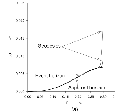
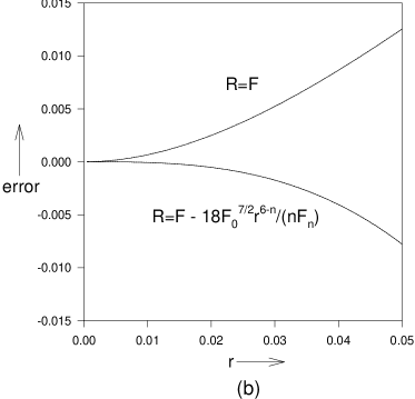
Figure 1: In this models density goes to zero smoothly at the boundary. The energy and mass functions are $f=0,\;F=r^{3}-2.5r^{4}$. a) Plots of different outgoing radial null geodesics terminating at the singularity in past. We clearly see the $R=F$ kind of behaviour for these geodesics near the singularity. b) graph showing error ${R_{actual}-R_{approximate}\over R_{actual}}$ against $r$ near the singularity for $R=F$ curve and the first corrected curve $R=F-{18F_{0}^{3.5}\over nF_{n}}r^{6-n}$.

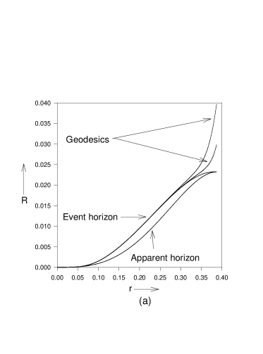
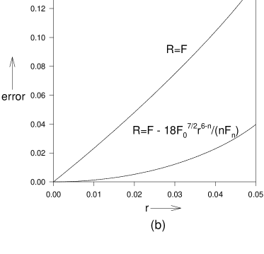
Figure 2: Density goes to zero smoothly at the boundary. The energy and mass functions are $f=0,\;F=r^{3}-2.5r^{5}$. a) Plots of different outgoing radial null geodesics terminating at the singularity. We clearly see the $R=F$ kind of behaviour for these geodesics near the singularity. b) The graph showing error ${R_{actual}-R_{approximate}\over R_{actual}}$ against $r$ near the singularity for $R=F$ curve and the first corrected curve $R=F-{18F_{0}^{3.5}\over nF_{n}}r^{6-n}$.

The Fig. 1 and Fig. 2 show the plots of the geodesics equations. Fig. 1 shows the plots for $F=F_{0}r^{3}+F_{1}r^{4}$, and Fig. 2 shows the plots for $F=F_{0}r^{3}+F_{2}r^{5}$. We have also plotted the apparent horizon, and the analytical form of the geodesic equation near the singularity with first correction to $F$ [4], i.e.

$$R=F-{18F_{0}^{3.5}\over nF_{n}}r^{6-n}$$

.

It matches very well the actual geodesic equations near the singularity. Fig. 1(b) and Fig. 2(b) show the error in analytical approximation against the numerical solution at different values of $r$ near the singularity. We see that the first corrected result to $F$ matches much better with the actual trajectories near the singularity. The plots also give strong numerical evidence that there is a family of RNGs meeting the singularity along the apparent horizon. The deviation of geodesics from each other seems to be very drastic as they move out. In other words, near the center all the singular geodesics converge very fast and fall on each other as predicted by our analytic calculation.

3.3 The timelike geodesics

Coming to timelike geodesics, by using the set of differential equations (9-14) for the geodesics, and using self-consistency requirements, the approximate solution for the timelike geodesics near the central singularity along the normal root direction ($R=X_{0}r^{\alpha}$) can be written as,

$$K^{t}={1+C^{2}\over 2C}\pm r^{1-n/3}{1-C^{2}\over 2C}\sqrt{F_{0}\over X_{0}}+higher\;order\;terms,$$ (22)

$$R(t,r)=X_{0}r^{1+2n/3},$$ (23)

Here $C\neq 1$ is a constant labeling different geodesics corresponding to the particles having different energies at a given point in spacetime, and the signs $\pm$ represent outgoing and ingoing geodesics. The case $C=1$ was discussed in [5]. So we see that when $C\neq 1$ the timelike and spacelike geodesics have the same limiting tangent at the singularity as that of the RNGs terminating at the singularity. Thus all the geodesics go along the same direction, which we would not have expected to happen typically.

Let us now look for timelike radial geodesics coming out of the central $(r=0)$ singularity along the apparent horizon, if they exist, i.e. with the behaviour $R=F_{0}r^{3}+\;higher\;ordered\;terms$. Assuming such geodesics to exist, and using the set of differential equations (9 - 14) for the timelike geodesics and solving them in an approximate manner near the singularity, we get,

$$K^{t}=C\;Exp{\bigg{[}}{-nF_{n}\over 3(3-n){F_{0}}^{5/2}}r^{n-3}{\bigg{]}}.$$ (24)

Here different values of $C$ represents different geodesics corresponding to the particles having different energies at a given point in the spacetime like in the earlier equation. We see that $K^{t}$ and $K^{r}$ blow up exponentially, making $K^{t}/K^{r}=1$, and to the lowest orders, near the singularity the $dR/dr$ equation becomes the same as that of the null geodesics. Along any other directions (i.e. apart from the larger root, which is the Cauchy horizon direction, and the apparent horizon direction, and the two special cases discussed earlier[5]), we get contradiction while solving the set of differential equations for the geodesics. That means these are the only possible behaviours for the geodesics near the singularity. And because $K^{t}$ diverges very rapidly near the central singularity, all the arguments and calculations given above for null geodesics also hold for timelike geodesics, i.e. families of timelike and null geodesics come out of the singularity along the apparent horizon direction near the central singularity. If one also solves the set of differential equations for spacelike geodesics in a self-consistent manner, then one can see that even the spacelike geodesics have a behaviour very similar to that of null geodesics near the central singularity.

Fig. 3 shows the timelike geodesics. Within a given range, timelike geodesics starting from the singularity can meet the boundary of the cloud at the same time with different velocities, and there is also a family of such geodesics which meet the boundary of the cloud at different times as shown in this Figure. This implies that in some region, at every point in the spacetime we have timelike geodesics coming out of the singularity with apparent horizon as tangent at the singularity and meeting that point with different velocities.

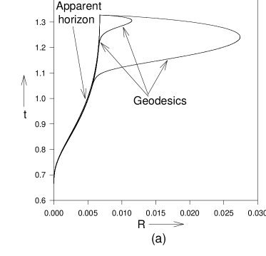
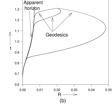
Figure 3: Different outgoing timelike geodesics for $f=0\;F=r^{3}-2.5r^{4}$. Density smoothly goes to zero at the boundary. All these geodesics show $R=F$ kind of behaviour near the singularity. Different timelike geodesics meeting the same point correspond to the particle having different velocities. a) Different timelike singular geodesics meeting the apparent horizon at the boundary. b) Different timelike singular geodesics meeting R=0.02 at the boundary.

Though we have considered here the marginally bound case $f=0$ for the sake of clarity and simplicity, the results are easily generalized for non-marginal cases as well. They essentially depend upon the value of the parameter $\alpha$ which is chosen such that $R^{\prime}/{r^{\alpha-1}}$ remains finite in the limit of approach to the singularity along the trajectories coming out. In the $\alpha<3$ cases, we again get a family of RNGs coming out of the singularity along the apparent horizon. This happens because in general along the outgoing RNGs (here for simplicity we discuss only null geodesics) $dR/dr^{3}=(1-\sqrt{f+F/R}/\sqrt{1+f})R^{\prime}/(3r^{2})$, so even with $f\neq 0$ we again have situations with $R=F+M_{\delta}r^{3+\delta}$, such that the first term in bracket goes to zero and the second term blows up but their product remains finite, giving the value of the tangent to be $F_{0}$.

Finally, we make here some remarks in order to clarify the situation regarding the strength of the naked singularity for the cases we have considered here. As we indicated earlier, the singularity in this model is always gravitationally strong[5]. We discuss this in some detail below.

The basic idea, in order to examine the strength of a singularity (naked or otherwise), is to examine the rate of curvature growth along the non-spacelike geodesics terminating in the singularity, in the limit of approach to the singularity. There are many criteria available for this purpose, as we point out below. According to the definitions of strength of a singularity as given by Tipler [8, 9, 10] there are two criteria given to check the strength. According to one definition, a divergence condition to be satisfied is, $R_{ij}V^{i}V^{j}$ should go as $1/k^{2}$ ($k$ is the affine parameter along the geodesic, vanishing in the limit of approach to the singularity) as one goes to the singularity, along every geodesic coming out, and also for the ingoing ones. According to the second definition of Tipler, the singularity is strong if this divergence condition is satisfied along at least one trajectory terminating in the singularity. We like to use this later definition of strength, because there is practically no way available to check the earlier definition operationally, because it is nearly impossible to integrate all non-spacelike geodesics in most of the collapse scenarios. Also, considering the complexity of the field equations, for most of the collapse models (consider e.g. the well-known case of Vaidya-Papapetrou radiation collapse), there is going to be some kind of a directional dependence always in the behaviour of the curvature growth in the limit of approach to the singularity. A uniform kind of curvature dependence in all directions does not seem plausible. Thus, it looks extremely reasonable to make the statement that the geodesic ends in a strong curvature singularity provided the curvatures grow as per the above requirement along it, rather than defining the strength as some kind of an absolute property of the singularity.

In fact, there are other criteria as well proposed and available to check the strength. For example, according to the criterion given by Krolak [11] (see e.g. [10]), a divergence $R_{ij}V^{i}V^{j}$ going as $1/k$ is sufficient to call the singularity strong. According to this criterion as well, clearly the naked singularities considered here are all strong curvature singularities along every null geodesic terminating in the singularity. There have also been some recent general considerations on strength by Nolan [12], according to which practically all shell-focusing singularities occurring in spherically symmetric spacetimes are gravitationally strong. Taking all these considerations into account, it would appear quite reasonable to treat the naked singularities considered here to be strong curvature ones, which are physically important and not removable from the spacetime in a classical manner.

4 Conclusion

We have explored here the behaviour of null geodesics in the vicinity of the naked singularity developing in the gravitational collapse of a dust cloud. Together with the earlier information available in this connection (especially in the case $n=3$), this provides a rather complete picture of how null trajectories traverse away from the naked singularity.

We also see that there are ingoing and outgoing timelike geodesics terminating at the central naked singularity, and they have a behaviour very similar to that of the null geodesics when near the central singularity. This is an intriguing phenomenon and because of this in many cases it may become difficult to decide whether a given vector is null, timelike or spacelike at the central singularity. This can happen because normally while doing calculations in such cases we finally use some approximations and take limits.

We further showed that there is a family of radial null (as well as radial timelike geodesics) coming out of the singularity with the same ultimate tangent as that of the apparent horizon, when the parameter $\alpha<3$, i.e. the geodesics have $R=F$ kind of behaviour as we approach the singularity. Very similar results can be obtained for spacelike geodesics also. For timelike geodesics in $\alpha=3$ case again we get results quite similar to that of null geodesics, as $K^{t}$ has a power-law divergence near the singularity. Even in collapse scenarios more general than dust we can expect a similar phenomenon, i.e. in the cases corresponding to $\alpha<3$, we expect a family of geodesics coming out with $R=F$ kind of behaviour as the general structure of $dR/dr$ equation looks very similar. These results provide us with an insight into the causal structure in the vicinity of the naked singularity.

We thank the referee for helpful comments on the paper. It is a pleasure to thank I. H. Dwivedi for discussions, and SSD would like to thank T. Harada, H. Iguchi, and K. Nakao for many useful comments.

References

- [1] R. C. Tolman, Proc. Natl. Acad. Sci. USA (1934), 410; H. Bondi, Mon. Not. Astron. Soc. (1947), 343; G. Lemaître, Ann. Soc. Sci.Bruxelles I, A53, 51(1933).
- [2] P. S. Joshi and I. H. Dwivedi, Phys Rev D 47, 5357 (1993); R. P. A. C. Newman, Class. Quantum Grav. , 527 (1986); D. Christodoulou, Commun. Math. Phys. , 171 (1984); D. M. Eardly and L. Smarr, Phys. Rev.D 19, 2239 (1979).
- [3] P. S. Joshi and T. P. Singh, Phys. Rev. D , 5357 (1995); Dwivedi I H and Joshi P S, Class. Quant. Grav. 14, 1223 (1997); S. Jhingan and P. S. Joshi, Ann. Isr. Phys. Soc. bf 13, 357 (1997).
- [4] S. S. Deshingkar, S. Jhingan, P. S. Joshi, Gen. Rel. and Grav. , 1477 (1998).
- [5] S. S. Deshingkar, P. S. Joshi, I. H. Dwivedi, Phys. Rev. D , 044018 (1999).
- [6] F. C. Mena, R. Tavakol, P. S. Joshi, Phys. Rev. D, To appear, (2000) (gr-qc0002062); H. Iguchi, K. Nakao, T. Harada, Phys. Rev. D57, 7262, (1998); H. Iguchi, T. Harada, K. Nakao, Prog. Theor. Phys. 101, 1235 (1999); H. Iguchi, T. Harada, K. Nakao, Prog. Theor. Phys. 103, 53 (2000); R. V. Saraykar and S. H. Ghate, Class. Quantum Grav. 16, 281 (1999), B. J. Carr and A. Coley, Class. Quantum Grav. 16, R31 (1999).
- [7] T. P. Singh and P. S. Joshi, Class. Quantum Grav. , 559 (1996).
- [8] Tipler F J Phys. Lett.67A 8(1977).
- [9] F. J. Tipler, C. J. S. Clarke, and G. F. R. Ellis (1980), in General Relativity and Gravitation, edited by A. Held (Plenum, New York), Vol. 2, p. 97.
- [10] C. J. S. Clarke (1993), The analysis of space-time singularities, (Cambridge University Press, Cambridge).
- [11] Królak A 1978 MSc Thesis, Singularities and Black Holes in General Space-times University of Warsaw, unpublished.
- [12] B. Nolan, Phys. Rev. D60,024014 (1999)