Effects of Pair Creation on Charged Gravitational Collapse

Abstract

We investigate the effects of pair creation on the internal geometry of a black hole, which forms during the gravitational collapse of a charged massless scalar field. Classically, strong central Schwarzschild-like singularity forms, and a null, weak, mass-inflation singularity arises along the Cauchy horizon, in such a collapse. We consider here the discharge, due to pair creation, below the event horizon and its influence on the dynamical formation of the Cauchy horizon. Within the framework of a simple model we are able to trace numerically the collapse. We find that a part of the Cauchy horizon is replaced by the strong space-like central singularity. This fraction depends on the value of the critical electric field, $E_{\rm cr}$, for the pair creation.

1 Introduction

The well known exact solution of the coupled Maxwell-Einstein equations outside the spherically-symmetric matter distribution is the Reissner-Nordstrøm solution. The analytic extension of the Reissner-Nordstrøm metric has rather exotic properties. The black hole’s interior contains Cauchy horizons, time-like singularities and tunnels to other asymptotically flat regions.

Recently, it has been shown both in perturbative analysis and by solving the full non-linear problem that a Cauchy horizon inside a charged black hole is transformed into a null, weak singularity [1, 2, 3, 4, 5, 6]. The Cauchy horizon singularity is weak in the sense that an infalling observer crossing it experiences only a finite tidal deformation [3, 4]. However, the curvature scalars diverge along the Cauchy horizon, leading to an unbound growth of the internal mass-parameter, a phenomena known as the mass-inflation [2]. The earlier studies were done on the pre-existing (eternal) Reissner-Nordstrøm space-time. Hod and Piran [7], have demonstrated explicitly that mass-inflation takes place also during a dynamical charged gravitational collapse. The dynamical space-time is drastically different from the analytically extended Reissner-Nordstrøm manifold: it resembles more the Schwarzschild one. The Penrose diagrams of the various space-times are depicted on Figure 1.

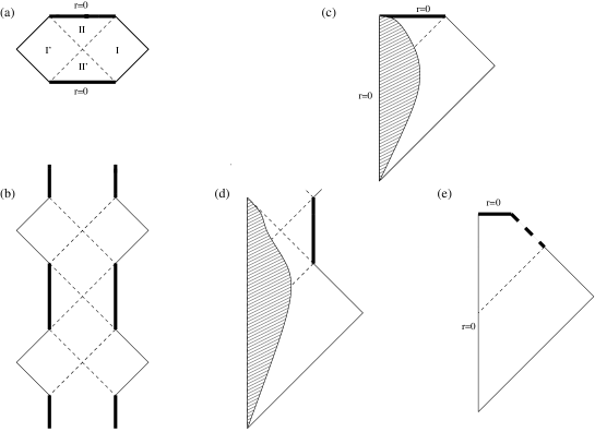
Figure 1: Penrose diagrams. $(a)$ and $(b)$ are, respectively, the Schwarzschild and the Reissner-Nordstrøm eternal (pre-existing) spacetimes , $(c)$ and $(d)$ are ones expected to form during a dynamical collapse of a neutral and a charged matter, respectively. The actual, dynamically calculated, space-time geometry for a charged gravitational collapse, $(e)$ is dramatically different from that depicted on $(d)$ and it resembles (in broad terms) the Schwarzschild space-time. In all the figures thick solid lines represent central singularities (space-like for the Schwarzschild manifold or time-like for the Reissner-Nordstrøm one). The weak, null singularity in figure $(e)$ is represented as a thick dashed line, while thin dashed lines describe various horizons.

This is so far the classical picture. Our goal, here, is to consider quantum effects and to investigate the influence of pair creation in strong electric fields on charged gravitational collapse. Specifically, we are interested in the effects of pair creation on the inner structure of the black hole that forms in such a collapse. This goal differs from previous works on the subject. Pair creation was mainly considered in the external region of a pre-existing black hole’s space-time, outside the event horizon [9, 10, 11, 12]. It has been shown that the produced particles rapidly diminish the charge of a black hole as seen by an external observer.

Particles creation takes place, however, also in the inner region of a black hole. Novikov & Starobinskiĭ [13] and Herman & Hiscock [14] studied the inner geometry and the stability of a Cauchy horizon in the pre-existing Reissner-Nordstrøm space-time influenced by the pair creation effect. The model in Ref. [14] assumes the instantaneous disappearance of the electric field, when the pair creation takes place inside the event horizon along $r_{\rm cr}=const$ hypersurface. The Reissner-Nordstrøm patch of the space-time exterior to this hypersurface is glued along the $r_{\rm cr}=const$ hypersurface to an interior Schwarzschild patch. In this model the Cauchy horizon does not exist. The model in Ref. [13] assumes an initially Reissner-Nordstrøm geometry and allows the evolution of the electric field through the back-reaction of the created pairs. In this model the initial Reissner-Nordstrøm geometry evolves to an uncharged, Schwarzschild-like one - the Cauchy horizon is shown to be unstable with respect to the process of pair creation. It should be emphasized that in this model the Cauchy horizon is assumed to be stationary $r_{\rm CH}=const$ hypersurface. This is in contrast to the recent investigations [1, 2, 3, 4, 5, 6, 7], where the Cauchy horizon was shown to be non static, contracting null hypersurface.

Although, the particle production in the intensive electric field is the simplest quantum process, its influence on the inner structure of black holes was not studied yet in an evolutionary context. The effect of pair creation in the intensive electric field is probably most important, when dealing with a formation of the inner structure of a charged black holes. This depends, of course, on the parameters of the formed black hole. In this work we take a different point of view from [13, 14] and explore the dynamical picture i.e., we replace the question is the Cauchy horizon stable, with the question does it form at all. To address this question, one should consider the collapse of a charged self-gravitating matter. The electron-positron pairs are produced in the electric field of the collapsing matter. To treat consistently the problem of such a collapse, one should take into account the back-reaction of the produced pairs on the source’s electric field. This is achieved by adding the electric current due to the produced pairs as a source to the Maxwell equations:

$${F^{\alpha\beta}}_{;\beta}=4\pi J^{\alpha}_{\rm free}+4\pi J^{\alpha}_{\rm pairs}\ .$$ (1)

The charge conservation equation in the situation with pair creation is modified by adding the charge source:

$${J^{\alpha}}_{;\alpha}=\Gamma(F^{\alpha\beta})\ .$$ (2)

The stress-energy of the electric current of the produced particles arises from the stress-energy of the electric field. The latter is the source of the pairs, by means of the energy-momentum conservation.

To formulate the problem properly we need a back-reaction formalism that includes the back reaction of the pairs on the stress energy tensor of the electric field that create them. Without this the problem would not be self consistent. Such a formalism is not available. Instead we consider here a toy model that utilizes the main physical properties of the system - the fact that the pairs limit the electric field to a critical value, $E_{\rm cr}$. We describe this effect of pair creation by introducing a nonlinear dielectric constant which prevents the electric field from exceeding $E_{\rm cr}$, the critical pair creating field. In doing so we have ignored the electric current of the pairs and their stress-energy. We also disregard the contribution from vacuum polarization, which becomes significant only for the exponentially large fields [8]. In spite of this simplifying assumptions we believe that this model captures the characteristic behavior of the real system.

In section 2 we consider discharge in a classical space-time and give the motivation of the investigation of the influence of the pair creation on the inner structure of charged black holes. In section 3 we present the underling physical model. We develop the formalism and discuss the applicability of the model. Section 4 describes our numerical scheme. The results are presented in section 5. We compare a classical charged gravitational dynamical collapse with a collapse with the discharge. We summarize our conclusions in section 6. We use units in which $c=G=\hbar=1$.

2 Discharge in a Classical Charged Space-time

When pairs are created in an asymptotically flat region one of the particles, having the same charge as the field’s source, is repulsed from the body and escape to infinity. The another member of the pair is attracted to the body, decreasing its charge. This occurs, for example, to pairs created in the field of a charged black hole, outside its event horizon. The black hole discharges rather quickly, until its external field becomes subcritical [9, 10, 11, 12].

A more interesting situation occurs when a significant pair creation takes place within the event horizon of a charged black hole. The newborn particles do not have a spatial infinity to escape to, they are trapped within the event horizon. In the Reissner-Nordstrøm manifold in the region between the outer and the inner horizons the area coordinate $r$ and the time change their roles. The vector $\partial/\partial r$ is now timelike, while the vector $\partial/\partial t$ is spacelike. The only non-vanishing components of the electromagnetic tensor are $F_{uv}=-F_{vu}$ and only $F_{rt}=-F_{tr}$ are nonzero. An infalling observer moving along $dt/d\tau=0$ world-line, in the region between the horizons, will experience a spatially homogeneous electric field, increasing in strength into the future (the $r$-coordinate decreases). The electric field has only a $\hat{t}$-component: ${\bf E}={q(r,t)\over r^{2}}{\partial\over\partial t}$, wherein the bold face denotes usual 3-vectors. The direction of the field lines in a regular Reissner-Nordstrøm space-time is from one singularity to the other (see Figure 2). The maximally extended Reissner-Nordstrøm space-time has a charge asymmetry in the sense that two external observers in the two past asymptotically flat regions, $I$ and $I^{\prime}$, see the black hole charged oppositely. The left-hand and the right-hand singularities seem to such observers to have opposite charges.

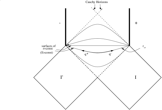
Figure 2: Pair creation inside the event horizon. Here we depict the Penrose diagram of the Reissner-Nordstrøm space-time. Pairs are produced when the electric field reaches the critical value $E_{\rm cr}$ along the surface $r=r_{\rm cr}$. Oppositely charged particles are accelerated in opposite directions, leading to the redistribution of the charge bellow the event horizon and to a change of the inner geometry of the charged black hole.

In the interior of a classical charged black hole, between the inner and the outer horuzons, pairs of charged particles are produced by the electric field along $r=const$ surfaces. An oppositely charged particles are accelerated in the opposite $\pm\partial/\partial t$ directions. Thus, if the black hole has a negative charge the positively charged particles will be attracted to it, accelerating toward the left-hand singularity, while the negatively charged particles will be repulsed from this singularity, accelerating toward the right-hand one (see Figure 2).

This leads to the redistribution of the charge, which was initially concentrated near the left-hand singularity. At the end of this process, in the perfectly symmetric situation, when the charge is equally divided among the left-hand and the right-hand singularities the electric field disappears. But the whole exotic structure of the inner part of the analytically extended Reissner-Nordstrøm manifold is due to the existence of this electric field. Therefore, vanishing of the electric field leads to the disappearance of the tunnels to other asymptotically flat regions. We will show here that a similar redistribution of the charge takes place also in a dynamical space-time, leading, as we shall see, to the partial closure of the “space tunnels”.

3 The Physical Model

In this section we develop an evolutionary formulation which includes the effect of pair creation in strong electric fields. We present bellow a simplified toy model, describing this effect for a dynamical space-time in which a black hole forms.

3.1 The Formulation

The first study of charged particles production in an uniform electric field was undertaken by J.Schwinger in 1951. The Schwinger’s formula for the number of scalar pairs created by the field $E$ per unit four-volume is:

$${\Gamma={e^{2}\over{2\pi^{2}\hbar^{2}c}}E^{2}\sum_{n=1}^{\infty}{(-1)^{n+1}\over{n^{2}}}\exp({-nE_{\rm cr}\over E})}\ ,$$ (3)

where $m$ and $e$ are the mass and the charge of a created particle and the critical electric field, $E_{\rm cr}$, is defined as:

$${E_{\rm cr}={\pi m^{2}c^{3}\over{e\hbar}}}\ .$$ (4)

The production rate of fermions differs from (3) by an overall factor $2$ and by the absence of the sign interchange $(-1)^{n+1}$.

The effect of the vacuum polarization (the change of the vacuum electric permittivity) in strong electric fields is instantaneously stronger than the contribution from a pair production ( by $\ln(E/E_{\rm cr})$ for $E\gg E_{\rm cr}$), but the latter can accumulate with the time [8]. The integrated contribution from the pair creation can dominate the contribution from the vacuum polarization.

Our model utilizes the essential property of the Schwinger’s result (3) - the exponential dependence on the ratio $E_{\rm cr}/E$, which means that pair creation rate is exponentially large for a supercritical field and the rate is exponentially suppressed for a subcritical field. This dependence suggests that once the field rises above $E_{\rm cr}$, charged pairs are produced intensively, reducing the field down to the critical value.

We neglect $(i)$ the net electric current of the pairs and $(ii)$ the stress-energy of the produced particles, assuming that the role of the electric current is confined to prevent the electric field from rising above the critical value. Hence, the electric field will be taken as:

$$E\equiv\left\{\begin{array}[]{r@{\quad\rm{if} \quad}l}E_{\rm ordinary}&E_{\rm ordinary}<E_{\rm cr}\\ E_{\rm cr}&E_{\rm ordinary}\geq E_{\rm cr}\end{array}\right.\ .$$ (5)

The $E_{\rm ordinary}$ stands for the ordinary electric field which would have arised in the absence of pair creation.

In this case we can mimic the effect of particles production as if the system was placed in a dielectric medium. Effectively, the polarization of this medium prevents the electric field $E$ from rising above $E_{\rm cr}$, while the electric displacement, ${\bf D}={\bf\epsilon}{\bf E}$, changes. The scalar quantity ${\bf\epsilon}$ is the dielectric constant. The electric displacement is related to the density of a free charge via the Maxwell equation:

$$\nabla\cdot{\bf D}=4\pi\rho_{\rm free}\ .$$ (6)

The dielectric “constant” that leads to (5) is given by:

$$\epsilon\equiv\left\{\begin{array}[]{r@{\quad\rm{if} \quad}l}1&E_{\rm ordinary}<E_{\rm cr}\\ |{\bf D}|/E_{\rm cr}&E_{\rm ordinary}\geq E_{\rm cr}\end{array}\right.\ .$$ (7)

The local description of the classical theory of electromagnetism in a curved space-time in a dielectric media can be derived from an effective local Lagrangian:

$${\cal L}^{\rm{(eff)}}=-{1\over 8\pi}{\bf E}\cdot{\bf D}=-{1\over 8\pi}{{|{\bf D}|}^{2}\over\epsilon}\ .$$ (8)

We use this Lagrangian with $\epsilon$ given by (7) to describe the effects of pair creation in the strong electric field.

Our toy model captures the essence of the physics, particularly the fast reduction of the supercritical field down to the critical value, $E_{\rm cr}$ and the energy-momentum conservation. The dielectric “constant” that we introduce has the same effect as the pairs which “shorten” an electric field above $E_{cr}$. However, we ignore all other features of the pairs, specifically we ignore the pairs themselves, their energy momentum tensor (which is replaced by a modified electromagnetic energy-momentum tensor that arises from the dielectric constant) and their electric current. This is done in order to obtain a simple self consistent energy conserving system. It is difficult to estimate what would be the effect of the electric current of the pairs. On the other hand it is clear that the stress-energy of the pairs would make a positive contribution to the mass-parameter (17) and will make the effects, which we describe latter, more pronounced.

Another artificial feature of our model is the ad hoc introduction of $E_{cr}$. This critical field is associated with the mass of the charged particles (see Eq. (4)). However, for simplicity our model is based on a massless charged scalar field, whose characteristics are along null geodesics. For such a massless field the critical electric field vanishes and charged massless pairs are produced even for an infinitely small electric field. We introduce a critical field $E_{\rm cr}$ as a free parameter which can be used to define the mass of the created particles trough the relation (4).

In addition to the above properties there are other minor and physically justified assumptions: First, our toy model ignores the contribution from vacuum polarization due to the intensive electric field (to be distinguished from the effective polarization, which we describe here). This would be justified if the effect of the vacuum polarization is small compared to the pair creation contribution. This is in fact the situation when the electric field is not exponentially large [8].

Second, when constructing our model, we have utilized Schwinger’s result (3), more precisely, its exponential dependence on $E_{\rm cr}/E$. Schwinger’s formula is valid, strictly speaking, only for an uniform and static electric field over a flat space-time background. The approximation of flat-space is valid if the radius of curvature of the dynamical geometry is much greater than the Compton wavelength of a created particles. The radius of a curvature can be taken of order $R^{-1/2}$, where $R$ is the Ricci curvature scalar. The Compton wavelength of the particles is $\ell={\left({\pi c\hbar\over eE_{\rm cr}}\right)}^{1/2}$. Thus, the condition for a flat-space approximation, $\ell\ll\ R^{-1/2}$, takes the form

$${\left({{\pi c\hbar\over eE_{\rm cr}}R}\right)}^{1/2}\ll 1\ .$$ (9)

But, the Ricci scalar $R$ has been shown, in dynamical models, to diverge approaching the Cauchy horizon, (this is the mass inflation scenario) thus, the approximation breaks down in vicinity of the singular Cauchy horizon. Notwithstanding, our model is, actually, not based on exact Schwinger result, but on its exponential dependence on $E_{\rm cr}/E$ which is non-perturbative.

Anyway, all approximations will be broken at some moment. Eventually, the curvature in the vicinity of the singular Cauchy horizon  becomes Planckian since the “Coulomb component” of the Weyl curvature diverges exponentially with advanced time (for a spherical symmetry- $|\Psi_{2}|\sim m/r^{3}$, with $m$ the internal mass parameter.) Moreover, the Ricci curvature may dominate the Weyl curvature and surpass the Planck values even earlier. In either case our analysis becomes meaningless, and a theory of quantum gravity is needed. We obviously consider only the sub-Planckian regions.

3.2 The Equations

Our goal is to integrate numerically the evolution equations and to follow the collapse of a spherically symmetric regular initial scalar field distribution via the formation of an apparent horizon and a Cauchy horizon, toward a central singularity. The conventional choice of coordinates for this dynamical evolution is double-null coordinates. In these coordinates: $(1)$ The apparent horizon (when it forms) is regular i.e. it is free from unphysical coordinate singularities; $(2)$ For a massless scalar field the characteristics are null so this choice is “natural” for models involving massless scalar fields.

We choose the line element of the form:

$${{ds}^{2}=-{{\alpha(u,v)}^{2}dudv}+{r(u,v)}^{2}d{\Omega}^{2}}\ ,$$ (10)

where $d{\Omega}^{2}$ is the unit two-sphere. There is a coordinate gauge freedom: the choice of coordinates ${u,v}$ is unique only up to a change of variables $v^{\prime}=f_{1}(v),u^{\prime}=f_{2}(u)$, which leave the line element (10) unchanged. For the time being we do not specify our double-null coordinates: these are just general ingoing and outgoing null coordinates. Later, when discussing the numerical integration we will fix the gauge freedom and specify the coordinates.

Let the $F_{\mu\nu}$ be the electromagnetic tensor, defined as $F_{\mu\nu}\equiv A_{[\nu;\mu]}$. In a spherically symmetric space-time the only non vanishing field components are: $F_{uv}=-F_{vu}$. Thus, only $A_{v}$ and $A_{u}$ need be non vanishing. Then $A_{v}$ can be removed by the gauge transformation $A_{\alpha}\rightarrow A_{\alpha}+\Lambda_{;\alpha}$ , with $\Lambda=-\int A_{v}dv$. We are left with $A_{u}\neq 0$ and we denote: $a(u,v)\equiv A_{u}$.

We reformulate the set of coupled Einstein-Maxwell-Scalar Field equations as a first order system. The numerical integration of the first order system functions very well both for the uncharged case, see Ref. [15], and for the charged situation [7]. It is convenient to define the auxiliary variables:

$$d\equiv{\alpha_{v}\over\alpha},\ f\equiv r_{u},\ g\equiv r_{v},\ s\equiv\sqrt{4\pi}\psi,\ w\equiv s_{u},\ z\equiv s_{v}\ ,$$ (11)

wherein $\psi$ is the complex massless scalar field. We have adopted the notation $W_{x}\equiv{\partial W/\partial x}$ for partial derivatives of any function $W=W(x,y)$.

We denote by $q(u,v)$ the free charge i.e. the charge of the collapsing scalar field, and by $\tilde{q}$ the total charge up to the sphere of radius $r$. The latter is the charge defined by the QED effects. The scalar field is collapsing under the influence of the total charge $\tilde{q}$ not the free charge $q$. In a local inertial frame: $q=\epsilon\tilde{q}$ and we define: $\tilde{a}\equiv a/\epsilon$.

We write the closed system of equations for the QED-corrected situation:

Einstein equations:

$$E1 \equiv rf_{v}+fg+{1\over 4}\alpha^{2}-{\alpha^{2}q^{2}\over 4\epsilon r^{2}}=0\ ,$$

$$E2 \equiv g_{v}-2dg+rz^{*}z=0\ ,$$

$$E3 \equiv d_{u}-{fg\over r^{2}}-{\alpha^{2}\over 4r^{2}}+{\alpha^{2}q^{2}\over 2\epsilon r^{4}}+{1\over 2}(wz^{*}+w^{*}z)+{1\over 2}ie\tilde{a}(sz^{*}-s^{*}z)=0\ .$$

Maxwell equations:

$$M1 \equiv \tilde{a}_{v}-{\alpha^{2}q\over 2\epsilon r^{2}}=0\ ,$$

$$M2 \equiv q_{v}-ier^{2}(s^{*}z-sz^{*})=0\ .$$

The scalar field equations:

$$S1 \equiv rz_{u}+fz+gw+ie\tilde{a}rz+ie\tilde{a}gs+{ie\over 4\epsilon r}\alpha^{2}qs=0\ ,$$

$$S2 \equiv rw_{v}+gw+fz+ie\tilde{a}rz+ie\tilde{a}gs+{ie\over 4\epsilon r}\alpha^{2}qs=0\ ,$$

and, finally, the definitions (11):

$$D1 \equiv d-{\alpha_{v}\over\alpha}=0\ ,$$

$$D2 \equiv g-r_{v}=0\ ,$$

$$D3 \equiv z-s_{v}=0\ .$$

The QED-corrected equations are reduced to the classical ones [7] by setting $\epsilon=1$.

3.3 The Characteristic Problem

The system of evolutionary equations have to be completed by a specification of the initial and the boundary data along some characteristic hypersurface. For models involving massless fields the characteristics are null segments. Thus, it is natural to specify the initial conditions and the boundary conditions along null hypersurfaces. A satisfactory, for an uncharged case, formulation of the initial-value problem has been given by Burko & Ori [16]. The generalization for a charged case is given bellow.

We choose the initial characteristic surfaces to be: the ingoing $v=const\equiv v_{i}$ hypersurface, and, the outgoing $u=const\equiv u_{i}$ hypersurface. If the domain of integration includes the origin of coordinates it leads to the necessity of a series expansion of physical quantities in powers of the proper distance from the origin, in a vicinity of $r=0$. We are, however, interested in the formation of the Cauchy horizon. We can, therefore, exclude the origin $r=0$ from the domain of integration. We achieve this by an appropriate choice of the final outgoing segment $u=const\equiv u_{f}$, so the domain of integration does not include the origin.

Now we can remove the coordinates freedom. To do so, we fix the “linear” gauge, i.e. we take $r$ to be linear with $u$ or $v$ along the characteristic hypersurfaces. Namely, on $u=u_{i}$ segment we choose $g\equiv r_{v}=1$, on $v=v_{i}$ segment we choose $f\equiv r_{u}=r_{u0}$. To get $r$ along initial surfaces it is necessary to supply $r_{0}=r(u_{i},v_{i})$ that serves as a free parameter.

The conventional choice for a characteristic segments $u_{i}=0$, $v_{i}=r_{0}$, yields:

$$r(u_{i},v)=v\ ,\ r(u,v_{i})=ur_{u0}+r_{0}\ .$$ (12)

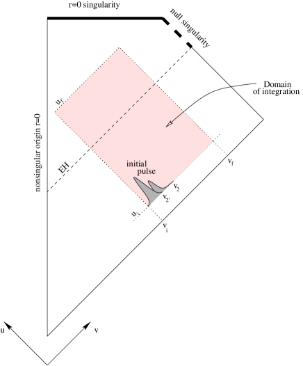
Figure 3: A schematic diagram of the integrated space-time.

Now we specify freely the scalar field distribution along the initial segments. We choose a compact ingoing scalar field pulse along the ingoing $u=u_{i}$ segment; and the “no-perturbation” along the initial outgoing $v=v_{i}$ segment. Specifically, we take $\psi(u,v_{i})\equiv 0$ that corresponds to a fixed static background for $v<v_{i}$. And we choose $\psi(u_{i},v)\equiv 0$ except at some finite region $v_{1}<v<v_{2},(v_{1}\geq v_{i})$. To be concrete, for a complex scalar field $\psi$, $\psi=\phi_{1}+i\phi_{2}$, with $\phi_{1},\phi_{2}$ two real scalar fields, we choose:

$$\phi_{1}={a\over{\sqrt{4\pi}}}\sin^{2}\left(\pi{v-v_{1}\over v_{2}^{\prime}-v_{1}}\right)\ ,\phi_{2}={b\over{\sqrt{4\pi}}}\sin^{2}\left(\pi{v-v_{1}\over v_{2}-v_{1}}\right)\ ,$$ (13)

where $a,b$ are constant amplitudes, and $v_{2}^{\prime},v_{2}$ are the end-points of each of the real-fields pulses, and $v_{1}=v_{i}$ is their common starting-point. This choice of the initial data is differentiable at the matching points $v_{1},v_{2}$. The integrated space-time is schematically depicted on Figure 3.

From (13) we obtain the initial values of $z$, and $w$:

$$z(u_{i},v) = {a\pi\over v_{2}^{\prime}-v_{1}}\sin\left(2\pi{v-v_{1}\over v_{2}^{\prime}-v_{1}}\right)+{ib\pi\over v_{2}-v_{1}}\sin\left(2\pi{v-v_{1}\over v_{2}-v_{1}}\right)\ ,$$

$$w(u,v_{i}) \equiv 0\ .$$ (14)

From the constraint equations E2-E3 and the definition D1, together with the choice $\alpha(u_{i},v_{i})=1$ one determines the initial values of $d$ and $\alpha$:

$$d(u_{i},v)={a^{2}\pi^{2}v\over 2(v_{2}^{\prime}-v_{1})^{2}}\sin^{2}\left(2\pi{v-v_{1}\over v_{2}^{\prime}-v_{1}}\right)+$$ (15)

$$+{b^{2}\pi^{2}v\over 2(v_{2}-v_{1})^{2}}\sin^{2}\left(2\pi{v-v_{1}\over v_{2}-v_{1}}\right)\ .$$

$$\alpha(u,v_{i})=1\ .$$ (16)

We assume the Minkowski space-time for $v<v_{i}$, therefore, we set $q(u,v_{i})=0$ and $a(u,v_{i})=0$.

In our coordinates the mass-function (the mass-parameter) becomes:

$$m(u,v)={r\over 2}\left(1+{q^{2}\over r^{2}}+{4\over\alpha^{2}}r_{u}r_{v}\right)\ .$$ (17)

Since the mass-function vanishes for the flat space-time (in the region $v<v_{i}$), one can calculate: $r_{u0}=-{1\over 4}$. It should be noted that for $v\gg m$ our ingoing null coordinate $v$ is closely related (proportional) to the ingoing Eddington-Finkelstein null coordinate $v_{\rm e}$. The $u$ coordinate is related to the proper time of an observer at the origin. This is defined as [15]:

$$T(u)=\int_{0}^{u}{\alpha(u^{\prime},u^{\prime})du^{\prime}}\ .$$ (18)

In our choice the space-time to the left to the $v=v_{i}$ characteristic hypersurface is Minkowskian until the very last moments of the collapse. Hence, $\alpha(u,u)=1$ except the section when $u\rightarrow u_{f}$, where $\alpha(u,u)\rightarrow 0$. Therefore, the integration in (18) is trivial and yields: $T(u)=u$. Later, we will find it useful to utilize the proper time of an observer at the origin as a measure of the “length” of the Cauchy horizon.

4 The Numerical Integration Scheme

We have converted the second order equations to first order equations. Our numerical scheme is based on a simultaneous integration of this first order system of coupled differential equations. We solve numerically equations $E1-E2,E4,M1-M2,S1-S2,D1,D3,D5$. We set $\epsilon=1$ to obtain the classical collapse with no pair creation.

The domain of integration is covered by a double-null grid. The characteristic initial-value problem is formulated in section 3.3. The algorithm for the numerical integration in the classical case ($\epsilon=1$) is described in [7]. Here we generalize this algorithm to the case when pair creation is included.

At each step we evolve $d$ and $z$ using $E3$ and $S1$ from the hypersurface $u$ to $u+du$. Then we solve the appropriate equations for the rest of quantities along the outgoing null rays $u+du=const$, starting from the initial outgoing hypersurface $v=v_{i}$. We integrate equation $D1$ to find $\alpha$, then we solve the coupled differential equations $D2$ and $E2$ to get $r$ and $g$. Next, the equations $D3,M2,M1$ are integrated to obtain $s$, $q$ and $\tilde{a}$. Finally, the differential equations $E1$ and $S2$ are solved for $f$ and $w$, respectively. After each step in the $u$-direction we calculate the electric field strength, $q/r^{2}$, along the current outgoing null ray ($u+du=const$). We use this field value to establish the value of $\epsilon$, according to (7), for the next $u$-step.

This integration scheme uses three distinct methods to evolve the initial data. All these methods are well known and commonly used (see, for example, the recipes-book by Press W.H., et al. [17]). To evolve the quantities in the $u$-direction we utilize the 5-th order Cash-Karp Runge-Kutta method. The differential equations in the $v$ direction are solved using a 4-th order Runge-Kutta method. The integrations in the $v$ direction are performed using a three-point Simpson method.

It is conventional to define the accuracy of a numerical method by the scaling of the numerical error. Thus, $n$th order accuracy means that, the error scales as the step-size to power $n$:

$$F_{\rm real}(x)=F_{\rm calc}(x)+O(h^{n})\ ,$$ (19)

where $F_{\rm real}$ stands for the actual value of a function at a point $x$, while $F_{\rm calc}$ for a calculated at the same point. The Runge-Kutta methods, which we utilize, are all at least second order accurate, see Ref. [17]. The three-point Simpson integration method is of order $n=4$.

We have performed a few simulations with the same free parameters, but with different grid sizes in order to check the scaling of the numerical errors. The numerical scheme proceeds in the $u$ and $v$ directions on grids with corresponding grid-spacings $h_{u}$ and $h_{v}$. These step-sizes are connected by the numerical stability requirement: $h_{u}\leq f(u,v)h_{v}$, where $f(u,v)$ is a slowly varying function of order unity. We perform the convergence test by changing the grids density in both directions.

$(a)$
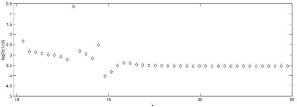
$(b)$      $(c)$

Figure 4: $(a)$ The error scaling indicates a quadratic or higher convergence except at a single point with $n=0.5$. $(b)$ To visualize the reason for loss of accuracy we give an approximate sketch of $r(u,v)$ as a function of $v$ for $u=const$, for different grid-densities. We give only a sketch and not the real plots, since in the latter the crossing is unobservable at these scales. $(c)$ Variation of the calculated $r(u,v)$ as a function of $v$, for certain value of $u$, for different grid-densities in a typical (with no line-crossing) region. The grid-densities are: $60$ grid-points per unit interval (solid line), $120$ grid-points (dotted line) and $240$ grid-points (dashed line).

In what follows, $F^{h}$ denotes the numerically calculated, with the numerical step-size of $h$, value of a function $F$ at some point. Here $h$ denotes the step-size in the $v$ direction. If the numerical scheme, involved in a calculation of $F^{h}$ is convergent, then the connection between the above quantities is given by (19). We performed a series of numerical simulations with doubled grid densities, or, equivalently, with halved step-sizes $h_{v}$ (and, therefore, with halved $h_{u}$) . We expect that: $F^{h}=F+O(h^{n})$. Now, defining $c_{1}\equiv F^{h}-F^{h/2}$, and $c_{2}\equiv F^{h/2}-F^{h/4}$, we expect that: $c_{1}/c_{2}=2^{n}$. Figure 4$(a)$ depicts $\log_{2}(c_{1}/c_{2})$ along an ingoing null $v$ coordinate, for a typical $u=const$ ray. It is clear from this Figure that in general $n\approx 3$, indicating a third order convergence.

One, however, notices the point $n\approx 0.5$, which indicates a very poor convergence. Moreover, the plot looks very variable in the region $12\leq v\leq 15$. The reason for this “jumpy” behavior is understood, if one looks closer at the function $F$ itself. We have used $F=r(u,v)$. We sketch on Figure 4$(b)$ the radius $r(u,v)$ along an $u=const$ outgoing null ray (see the next section). This sketch is magnified, since the actual plots of $r$ for different grid densities are indistinguishable on this scale. In the marked box one observes the crossing of curves for different grid densities. This crossing leads to a decrease of the convergence order. Notably, after this crossing the convergence returns to the high order.

Figure 4$(c)$ displays the variation of the calculated $F$ as a function of $v$ along a typical $u=const$ ray for different grids densities. The observed picture confirms the convergence.

5 Results

5.1 Classical Charged Collapse

We begin with verifying our numerical code for a classical collapse, a collapse without quantum effects. We set $\epsilon=1$. We fix the free numerical parameters to define the problem: $a=0.5,b=0.461,v_{i}=r_{0}=10,v_{f}=90,v_{2}=16,v_{2}^{\prime}=20,e=0.15$. The number of grid-points along outgoing and ingoing rays is of order of $10^{2}$ per unit interval. We follow the evolution of the regular initial data via the formation of an apparent horizon and a Cauchy horizon, toward the central singularity. For this specific choice of free parameters the resulting black hole has a charge-to-mass ratio, $q/m\approx 0.98$, in geometrical units.

Figure 5 displays the metric function $r(u,v)$ as a function of the ingoing coordinate $v$ for different values of the outgoing null coordinate $u$. One can distinguish between two kinds of rays: the outer and the inner rays. The outer rays, outgoing rays at small $u$, escape to infinity: $r(u,v\rightarrow\infty)\longrightarrow\infty$. Increasing $u$, one finds the first outgoing ray, which does not escape to infinity, but tends to a constant value. This ray indicates the event horizon, which asymptotically coincides with the apparent horizon. The ray becomes vertical at about $r\approx 16$ (not displayed). Increasing $u$ further, one steps into the inner region of the integrated space-time. Outgoing rays in this region approach a constant radius, depending on $u$, in asymptoticly late advanced times $v\rightarrow\infty$. This indicates the formation of a Cauchy horizon. Following the evolution of the space-time, the solution approaches the origin, $r=0$. Since our code is not constructed to include the origin we stop at $u_{f}$, before the integration reaches the origin.

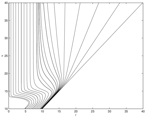
Figure 5: Radius $r(u,v)$ as a function of $v$ along $u=const$ rays. The retarded time $u$ increases from the initial straight ray toward the origin (from the right to the left), indicating the course of evolution of the space-time.

The main feature seen here is the existence of a contracting Cauchy horizon. The Cauchy horizon is not a stationary $r_{\rm CH}=const$ hypersurface as in the case of a classical Reissner-Nordstrøm space-time, but it depends on the outgoing null coordinate $u$, namely, it contracts toward the origin $r=0$ in late retarded time $u$.

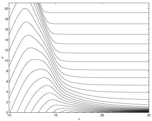
Figure 6: Lines of constant radius in $uv$-plane. The radius decreases from the bottom toward the top of the Figure. The apparent horizon, along which $r_{v}=0$, separates the exterior and the interior of the black hole. The latter region contains the Cauchy horizon.

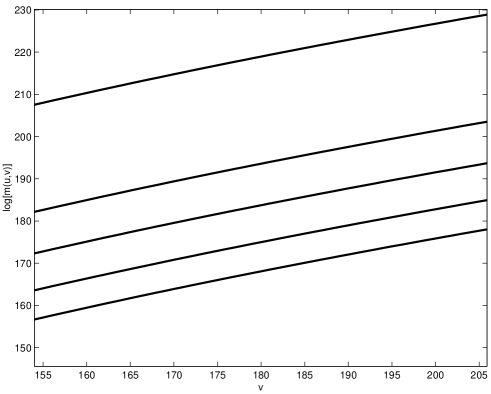
Figure 7: Logarithm of the mass-function, $m(u,v)$, vs. $v$ along $u=const$ null rays. The linear dependence of $m(u,v)$ on late time $v$ indicates the mass-inflation. The retarded time $u$ increases toward the top of the Figure.

Figure 6 depicts constant radii contour lines in the $uv$-plane. The bottom of the Figure ($u=0$) is the initial regular hypersurface. Looking along the $u$ direction one soon observes the formation of an apparent horizon, along which $r_{v}=0$. The apparent horizon separates the two regions with $r_{v}>0$ (on the left), and $r_{v}<0$ (on the right). The latter contains, also, the asymptotically ($v\rightarrow\infty$) constant, $u$ dependent section $r_{\rm CH}=const(u)$, representing the Cauchy horizon. The Cauchy horizon  itself is a null hypersurface which is approached as $v$ goes to infinity.

We depict the logarithm of the mass-function (17) in Figure 7, for a sequence of $u=const$ null rays. The straight lines indicate the exponential dependence of the mass-function on $v$ for late advanced times. The exponential growth confirms the conclusion that a mass-inflation indeed takes place in this collapse.

We have performed simulations with different free parameters: changing the amplitudes $a$ and $b$, the elementary charge $e$, stretching and squeezing the domain of integration. In all these cases we have not seen any qualitative difference between the results. The results, which we have obtained, are in excellent agreement with the previously established results, and fit well those in [7]. We conclude, thus, that our numerical code gives correct results to this case. We turn now to the problem of collapse with pair creation.

5.2 Collapse with Pair Creation

The critical electric field, $E_{\rm cr}$, is an additional free parameter in the problem with pair creation. The critical field strength $E_{\rm cr}$ is chosen in the forthcoming graphs so that it is reached just after the formation of the apparent horizon. This choice is arbitrary. Other comparable values of $E_{\rm cr}$ lead to a qualitatively similar results, unless $E_{\rm cr}$ is reached long before the formation of the apparent horizon (see bellow).

Figure 8 displays the radius $r(u,v)$ as a function of $v$ for a sequence of $u=const$ null rays. This Figure is analogous to Figure 5 for the classical situation. On a first sight these Figures seem very similar. There are, however, obvious differences, both qualitative and quantitative. A closer look uncovers the different incline of the late retarded rays ($u\rightarrow u_{f}$): while these rays depicted on Fig. 5 are practically vertical, those on Fig. 8 have an observable incline toward the origin $r=0$. The very last ray on the latter Figure, has an apparent tendency toward the origin, indicating that the $r=0$ strong singularity is close. Other signs of the difference between the two situations are quantitative ones. The whole “life-time” (in terms of the retarded $u$-time) of the QED-corrected system, before it hits the $r=0$ singularity is significantly shorter than the “life-time” of the corresponding classical system. For example, for the set of free parameters (see at the beginning of the previous section) the evolution of the QED-corrected system lasts $u_{f}\approx 12$, while for a classical system it takes about $u_{f}\approx 21$, before it crushes into the $r=0$ singularity. We note that $u_{f}$ is the proper time of an observer at the origin (18).

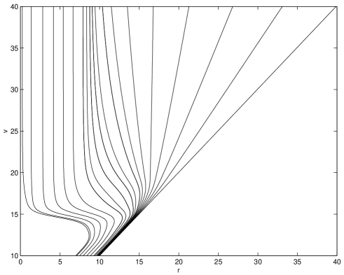
Figure 8: The radius, $r(u,v)$, as a function of $v$ along $u=const$ rays for collapse with pair creation. The retarded time $u$ increases to the left. One still observes the formation of the Cauchy horizon Ṫhere is also an apparent incline of the late retarded rays toward the origin, indicating discharge and signaling the destruction of the Cauchy horizon.

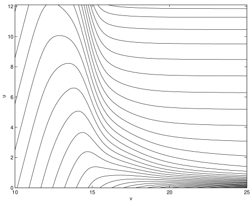
Figure 9: Contour lines of constant radius in $uv$-plane for a collapse with pair creation. The radius decreases from the bottom toward the top of the Figure. One observes the apparent horizon and the Cauchy horizon .

Figure 9 displays the contour lines of constant radii in the $uv$-plane. This Figure is analogous to Figure 6 for the classical situation. Again one can observe a different incline of the contour lines in the late retarded and advanced time regions. This difference in the incline between the classical and the QED-corrected problems can be interpreted as just a close approach to the intersection of the Cauchy horizon with the strong space-like $r=0$ singularity during the numerical simulation. The straightening of the outgoing rays occurs later in terms of the advanced $v$-time: the curvature is high in the vicinity of the strong singularity turning the rays toward the singular origin. The discharge is more apparent in the situation when the black hole, as it seen from infinity, has the small charge-to-mass ratio, see Figure 10.

We define the “length” of the Cauchy horizon as a proper time of an observer at the origin between the moment when he or she emits a last outgouing light signal that escapes to infinity (the event horizon) and the moment when he or she emits a first outgoing light signal that unavoidably falls into the spacelike singularity. This “length” is related to the retarded time $u$, see (18). We observe, therefore, that in the collapse with discharge the “length” of the Cauchy horizon is “shorter”, compared to the classical case.

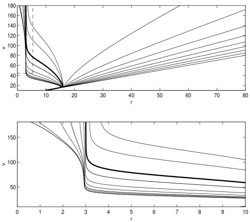
Figure 10: The radius $r(u,v)$ vs. $v$ along a sequence of $u=const$ rays in the situation when the charge-to-mass ratio, seen from infinity, of the formed black hole is small compared to unity. The bottom panel displays an enlargement of the marked region on the top panel. The rays’ incline toward the origin is apparent, indicating the discharge. The heavy line marks the beginning of the discharge.

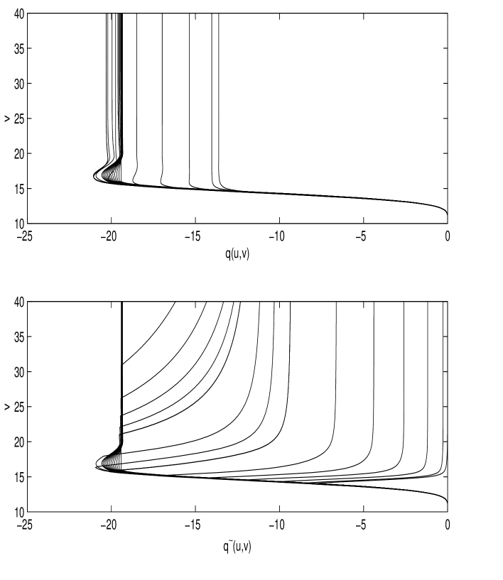
Figure 11: Top panel: the free charge $q(u,v)$ along $u=const$ null rays. Bottom panel: the total charge ${\tilde{q}}(u,v)$ along the same $u=const$ null rays. On both panels the retarded $u$ time increases from the leftmost ray toward the rightmost ray.

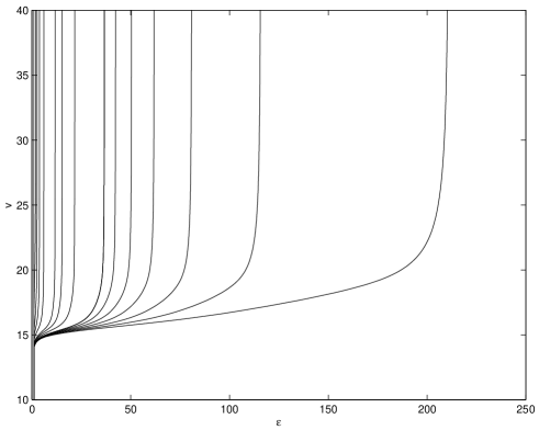
Figure 12: The dielectric constant $\epsilon(u,v)$ vs.$v$ along $u=const$ null rays. The retarded $u$ time increases from the left to the right. The dielectric constant, which represents the “polarization” field, grows with time $u$.

On the top panel of Figure 11 we depict the free charge $q(u,v)$ as a function of the advanced time $v$ along $u=const$ rays. The bottom panel of Figure 11 displays the total, QED-corrected, charge ${\tilde{q}}(u,v)$ along the same $u=const$ outgoing surfaces. The common characteristic property of the graphs is the straightening of the $u=const$ rays in late advanced times, when approaching the formed Cauchy horizon. The $u=const$ rays intersect the Cauchy horizon  as $v\rightarrow\infty$ and for different $u$ values the intersection occurs in different points with $r_{\rm CH}=const(u)$. Hence, a charge measured along an outgoing null rays approaches a constant $u$-dependent value which decreases with $u$, indicating a contraction of the Cauchy horizon  to the $r=0$ singularity. The difference between the graphs is the strong decay of the charge in the QED-corrected case relative to the classical case. In the former one, the charge approaches a maximum, which is defined by the strength of the critical field $E_{\rm cr}$, and then it is reduced by the created pairs keeping the electric field at constant $E_{\rm cr}$ value. After the pair creation process brought the charge to the “right” value, according to (7), the charge remains constant along an outgoing $u=const$ rays going toward the Cauchy horizon. Moreover, one observes the decrease to nearly zero charge on the bottom panel, in contrast to the classical situation.

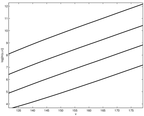
Figure 13: The logarithm of the mass-function, $m(u,v)$ vs. $v$ along a sequence of $u=const$ null rays. Again, the linear dependence of $m(u,v)$ on the late time $v$ indicates the mass-inflation. The retarded time $u$ grows from the bottom to the top.

The effective dielectric constant $\epsilon$ is depicted as a function of the advanced time $v$ in Figure 12. We note the growth of $\epsilon(u,v)$ with the lapse of the retarded time $u$ (the rightmost ray in Figure is the late $u=const$ depicted ray, the leftmost ray is the early $u=const$ ray). This is readily understood: the electric displacement ${\bf D}$ is growing and in order to keep the electric field at the constant $E_{\rm cr}$ value, the polarization field, represented by $\epsilon$, must grow, also.

In Figure 13 we depict the logarithm of the mass-function $m(u,v)$ along a sequence of $u=const$ outgoing null rays. The exponential dependence is clear, indicating that a mass-inflation takes place also in the collapse with the pair creation.

In the simulations presented so far $E_{\rm cr}$ was chosen such that $E_{\rm cr}$ was reached just after the apparent horizon forms. We have also performed simulations in which the critical field was reached $(i)$ long before or $(ii)$ long after the apparent horizon formed. Figure 14(a) displays the space-time of the black hole which is formed in the situation $(i)$. In this case the discharge begins long before the black hole forms. The charge of the black hole is very small, $q\ll m$. Therefore $r_{-}\approx{Q^{2}\over Mc^{2}}\ll r_{+}$ and the Cauchy horizon is unobservable, i.e. it forms (if at all) in the domain of very high (Planck) curvature. Figure 14(b) displays the space-time of a black hole which is formed in the situation $(ii)$. In this case the picture is very similar to the classical one. The pair creation begins at a very late stage when a significant part of the Cauchy horizon is already formed. The created pairs affect only the last stages of the evolution and the full formed Cauchy horizon is only slightly shorter than in the classical situation.

$(a)$
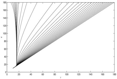
$(b)$

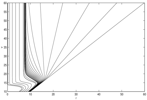
Figure 14: The radius $r(u,v)$ vs.$v$ along a sequence of $u=const$ rays in two situations: (a) The discharge begins at an early moment of collapse - the Cauchy horizon is unobservable and late rays are falling to the origin; (b) The discharge begins deep inside the apparent horizon of the black hole. The Cauchy horizon is almost unaffected relative the corresponding classical situation.

6 Summary, Conclusions and Outlook

We have constructed a dynamical model of a collapse of self-gravitating electrically charged massless scalar field including pair creation in strong electric fields.

Previous studies of the problem were concerned with particles production in the electric field: $(i)$ outside [9, 10, 11, 12] or $(ii)$ inside [13, 14] the event horizon of a pre-existing charged black hole. Here, we have formulated the problem in a way allowing us to address the question of the influence of the QED-effects on a formation of black holes within the framework of an evolutionary model. Our particular interest was devoted to a dynamical formation of the Cauchy horizon.

We have presented and used a toy model that treats the effect of pair creation in strong electric fields as an appearance of a local effective dielectric constant. The characteristic field strength $E_{\rm cr}$ describing the quantum effects in external field is viewed as a boundary between the classical and the quantum stages of the system’s evolution. We have simulated the collapsing matter by a massless scalar field. Hence, this critical field $E_{\rm cr}$ was set as a free parameter which defined the mass of the created particles according to (4). The conclusions from the numerical integration are presented below.

If the critical electric field strength is reached long before the formation of an apparent horizon almost complete discharge of the collapsing matter takes place and the final black hole is an almost neutral Schwarzschild black hole, see Figure 14(a). The black hole’s charge, as is measured from infinity is not strictly zero. The remaining charge is of order $E_{\rm cr}M^{2}$, where $M$ is the mass of the black hole.

If the critical value $E_{\rm cr}$ is approached after the apparent horizon forms the black hole seems from outside to have all its initial charge. Nevertheless, the process of discharge takes place in the inner region of a black hole. In the classical collapse strong central Schwarzschild-like singularity, and a weak singular Cauchy horizon is formed. With pair creation only a fraction of the Cauchy horizon remains a weak, null singular. The rest is replaced by a strong spacelike singularity. The “length” (as defined in section (5.2) of this weak singular section of the Cauchy horizon depends on the critical field strength $E_{\rm cr}$.

It is interesting to consider the interplay between the pair creation effects considered here and Planck scale quantum-gravity physics. There are two “extreme” situations: $(i)$ The critical field is reached deep inside the inner region, in the Planck region surrounding the central singularity. Then the Cauchy horizon is unaffected (or, it is unclear how the horizon is affected at the Planck scales) by the pair creation effect. It remains just the same as in a classical collapse (see Fig. 14(b)); $(ii)$ The critical field is reached at some moment before the formation of the apparent horizon then the Cauchy horizon is not formed at all (see Fig. 14(a)). More precisely, as it seen by an infalling observer, the formation of the Cauchy horizon occurs on the Planck scale. That is, from a practical point of view the Cauchy horizon does not form, cf. [13]. Between two extremes $(i)-(ii)$ the “length” of a weak singular, null section of a Cauchy horizon varies between a full, classical “length” and zero.

It should be emphasized that even if the critical field is approached before the formation of an apparent horizon , but after the moment $(ii)$, the weak, null singular section of a Cauchy horizon survives. This section is the familiar null singularity, and an internal mass-parameter diverges exponentially approaching it (see Fig. 13). We observe in the simulations the formation (or the lack) of a Cauchy horizon in various situation, mentioned before.

A charged spherically symmetric collapse is not a generic phenomena in the nature. One does not expect, in general, a significant excess of charge. But even if this not a case, the initially charged self-gravitating matter distribution will be rapidly neutralized by an accretion of an inter-stellar matter and by the pairs creation process.

A more generic phenomena of a collapse is one endowed by an angular momentum. This is an axisymmetric process and it is rather difficult to study, both analytically and numerically. The common property of a charged spherically symmetric collapse and the general axisymmetric one is an existence of Cauchy horizons inside the black hole. Hence, we use the charged collapse as a toy model to simulate the more general rotating situation and to derive a conclusions about the inner structure of the spinning black holes.

It would be interesting question to apply the considerations of this work to a local production of particles below the event horizon of a rotating black hole. Outside the event horizon of a rotating black hole the coupling of the black hole’s spin to the orbital angular momentum of particles leads to the phenomena of superradiance. If this process takes place below the event horizon of a spinning black hole, then this may lead to a destruction of a Cauchy horizon, just like in a charged case.

ACKNOWLEDGMENTS We thank S. Hod and S. Ayal for helpful discussions. The research was supported by a grant from the Israel Basic Research Foundation.

References

- [1] W.A. Hiscock, Phys. Lett A83, 110 (1981)
- [2] E. Poisson and W. Israel, Phys. Rev. D41, 1796 (1990)
- [3] A. Ori, Phys. Rev. Lett. 67, 789 (1991)
- [4] A. Ori, Phys. Rev. Lett. 68, 2117 (1992)
- [5] P.R. Brady and J.D. Smith, Phys. Rev. Lett 75, 1256 (1995)
- [6] L.M. Burko, Phys. Rev. Lett 79, 4958 (1997)
- [7] S. Hod and T.Piran, Phys. Rev. Lett. 81, 1554 (1998); Gen. Rel. Grav. 30, 1555 (1998).
- [8] A.A. Grib, S.G. Mamaev, V.M. Mostepanenko, Quantum Effects in Strong Fields, Atomizdat, Moscow, 2nd ed. 1988 (in Russian).
- [9] W.T. Zaumen, Nature, 247, 530 (1974);
- [10] B. Carter, Phys. Rev. Lett. 33, 558 (1974);
- [11] G.W. Gibbons, Commun. Math. Phys. 44, 245 (1975);
- [12] T. Damour and R. Ruffini, Phys. Rev. Lett. 35 , 463 (1975).
- [13] I.D. Novikov and A.A. Starobinskiĭ, Sov. Phys. JETP 51, 1 (1980).
- [14] R. Herman and W.A. Hiscock, Phys. Rev. D 49, 3946 (1994).
- [15] R.S. Hamadé and J.M. Stewart, Class. Quantum Grav. 13, 497 (1996).
- [16] L.M. Burko and A. Ori, Phys.Rev. D 56, 7820 (1997).
- [17] W.H. Press, S.A. Teukolsky, W.T. Vetterling and B.P. Flannery, Numerical Recipes in Fortran: The Art of Scientific Computing, 2nd ed. Cambridge University Press 1992.