Slowly Rotating General Relativistic Superfluid Neutron Stars

Abstract

We present a general formalism to treat slowly rotating general relativistic superfluid neutron stars. As a first approximation, their matter content can be described in terms of a two-fluid model, where one fluid is the neutron superfluid, which is believed to exist in the core and inner crust of mature neutron stars, and the other fluid represents a conglomerate of all other constituents (crust nuclei, protons, electrons, etc.). We obtain a system of equations, good to second-order in the rotational velocities, that determines the metric and the matter variables, irrespective of the equation of state for the two fluids. In particular, allowance is made for the so-called entrainment effect, whereby the momentum of one constituent (e.g. the neutrons) carries along part of the mass of the other constituent. As an illustration of the developed framework, we consider a simplified equation of state for which the two fluids are described by different polytropes. We determine numerically the effects of the two fluids on the rotational frame-dragging, the induced changes in the neutron and proton densities and the inertial mass, as well as the change in shape of the star. We further discuss issues regarding conservation of the two baryon numbers, the mass-shedding (Kepler) limit and chemical equilibrium.

I Introduction

For very practical reasons, past modeling of general relativistic neutron stars has largely relied on a one-constituent perfect fluid approximation to describe the stress-energy of matter. This would be appropriate if neutron stars truly consisted solely of neutrons in a fluid state. However, this is a drastic oversimplification. In reality a neutron star is composed of many different constituents and is best described as a “layer-cake”. A few seconds after it is born in a supernova a neutron star cools below $10^{10}$ K. Then the outer layers (with densities below, say, $1.5\times 10^{14}$ g/cm³) will “freeze” into a solid crust. After a few months of further cooling, the star will reach the critical temperature at which the bulk of the neutrons at densities above neutron drip ($\sim 10^{11}$ g/cm³) become superfluid. At roughly the same time the protons (expected to make up a few percent of the core material) may become superconducting. Thus, even in the simplest reasonable model a neutron star contains a thin fluid ocean, the roughly 1 km deep solid crust mentioned above, and a core containing superfluid neutrons, (potentially superconducting) protons and electrons. The lattice of nuclei and electrons in the inner crust is permeated by superfluid neutrons. Yet more complex models would allow for the presence of exotic particles in the core (eg. hyperons), high density phase-transitions to kaon and/or pion condensates and/or regions with deconfined quarks [1].

Despite these many complexities the perfect fluid approximation is reasonable when all the constituents flow together (see, for instance, Comer and Langlois [2]). However, it can never accomodate situations where the superfluid neutrons flow “independently” of the protons. Since this is, in fact, expected to be the case in a real neutron star the standard approach has serious deficiencies. During the last twenty years there have been continued attempts to piece together a coherent picture of neutron star superfluidity, using a variety of theoretical arguments and imposing observational constraints based on glitch and cooling rate data. Of particular interest for our present discussion are issues regarding the coupling between the superfluid and the normal fluid constituents, the main question being whether the superfluid neutrons will co-rotate with the protons or not. The answer to this seemingly innocent question is very complicated, but the current consensus is that even though the two fluids are strongly coupled they can sustain a state of differential rotation over significant timescales.

Alpar et al [3] have shown that the charged components in the core fluid (the protons and the electrons) will be strongly coupled to the crust nuclei via electromagnetic interactions. This suggests that a superfluid star can be described in terms of two fluids: one that represents the superfluid neutrons and one that describes all charged components (protons, electrons, crust nuclei etc.). In the following we will refer to these two fluids as the “neutrons” and the “protons”, respectively. Furthermore, in a rotating star the normal fluid constituent will settle into an essentially non-dissipative configuration on the viscous timescale. This implies that the “protons” must rotate uniformly (with proton angular velocity $\Omega_{p}=$ constant). This is not a priori the case for the neutrons since a (pure) superfluid is non-dissipative. In other words, one can conceivably have a stationary configuration with differentially rotating neutrons (with neutron angular velocity $\Omega_{n}\neq$ constant). This would certainly be true if the two fluids were completely uncoupled but, in reality, this is likely not the case. In order to begin to understand what really happens we need to discuss a non-dissipative mechanism known as the entrainment effect and how it leads to a dissipative mechanism called mutual friction.

In a mixture of the two superfluids Helium three and Helium four, it is known that the momentum of one of the constituents carries along (or entrains) some of the mass of the other constituent [4, 5]. The analog in neutron stars is an entrainment of some of the protons, say, by the neutrons. A superfluid is by its very nature locally irrotational [6], so when neutron stars rotate they do so via the formation of a dense array of quantized vortices. Because of entrainment the flow of neutrons around these vortices will induce a flow also in a fraction of the protons. This leads to magnetic fields being formed around the vortices. Due to the electromagnetic attraction of the electrons to the protons (the timescale of which is very short) there will then be a dissipative scattering of the electrons. In the context of oscillating superfluid stars this dissipative mechanism is known as mutual friction.

Much of the discussion of neutron star superfluids concerns attempts to theoretically model the observed glitches. The favoured model has long been based on the idea that the glitches correspond to a transfer of angular momentum from the superfluid that permeates the crust to the lattice. This picture is attractive since

$${\Delta\dot{\Omega}\over\dot{\Omega}}\sim{\Delta I\over I}\sim 10^{-2}-10^{-3}$$

where $\Delta\dot{\Omega}/\dot{\Omega}$ is the observed relative change in spindown rate and $\Delta I/I$ is the fraction of the total moment of inertia contained in the crustal superfluid. Furthermore, it has been argued that the time-scale on which the core superfluid couples to the charged component (in our case, the time on which neutron rotation rate becomes equal to that of the protons) is short (on the order of 1-10 s). For example, Alpar and Sauls [7] argue that, if $P$ is the period of rotation of the bulk of the matter of the neutron star in units of seconds, then on timescales of $4\times 10^{2}-10^{4}~{}P$ any difference of rotation between the neutrons and protons in the core will be damped out because of the entrainment effect and mutual friction. The consequence then is that only the inner crust superfluid would be able to rotate at a different rate from the rest of the star on a timescale beyond at most a few minutes.

However, there are many uncertainties in this game, e.g. the strength of the vortex pinning and the exact parameters for entrainment, and it is not at all clear that the standard picture is correct. In fact, recent work casts some doubt on its validity. To see this, we follow Langlois et al [8] and quantify the coupling timescale in the following way:

$$\tau\sim{1\over 2}\left(c_{r}+c_{r}^{-1}\right)\left(1+{I_{n}\over I_{p}}\right)^{-1}{1\over\Omega_{n}}$$ (1)

where $I_{n}$ and $I_{p}$ are the moments of inertia of the neutrons and the protons, respectively, and $c_{r}$ is the “drag to lift ratio” that depends on the relative rotation rate. This estimate is convenient because it describes the lifetime of a local difference in angular velocity of the two fluids in terms of a single parameter. As is immediately clear from (1) the timescale is short if $c_{r}$ is roughly of order unity (when the “drag” resulting from entrainment is of the same order as the Magnus force that acts on the vortices), while it becomes long if $c_{r}>>1$ or $c_{r}<<1$. Now, recent estimates of the strength of the pinning of the superfluid vortices to the nuclei in the inner crust suggest that $c_{r}$ is small in this region (leading to a relaxation time of $\sim 50$ days) [9]. Additionally, a detailed investigation of the scattering of electrons off of proton vortex clusters [10] in the core suggests that $c_{r}$ is very large there. In other words, it would seem plausible that the superfluid components relax towards co-rotation with the normal fluid rather slowly—both in the crust and deep in the core. This would indicate that differential rotation between the superfluid neutrons and the “protons” can be sustained on timescales of days to years.

Clearly, this is a problem where we are far away from a final conclusion at this point in time. Fortunately, this does not matter for the present discussion. It is clear that even if the coupling between the two fluids is strong, differential rotation should prevail on a time-scale orders of magnitude larger than the dynamical one ($\sim$ ms). Further evidence for this may follow from observed temperatures of millisecond pulsars. We recall attempts to explain the observations in terms of frictional heating due to differential rotation between the superfluid and the crust [11]. This discussion typically suggests that roughly 1% of the total moment of inertia (eg. the superfluid in the inner crust) must rotate differently from the rest of the star, in such a way that $10^{-2}\mbox{ rad/s}\leq|\Omega_{n}-\Omega_{p}|\leq 10\mbox{ rad/s}$. This would lead to a significant internal heating that would be relevant after the neutrino cooling era.

It is also worth mentioning that one should be careful before concluding that the coupling between the two fluids will necessarily lead to a co-rotating system. As argued by Langlois et al [8], this is unlikely to happen in cases when an external torque is acting on the system. Then the difference $\Omega_{n}-\Omega_{p}$ will stabilize at a value that represents a balance between the acting torque and angular momentum redistribution in the fluid. Since the external torque acts on the crust which then exerts a drag on the superfluid, we would typically expect $\Omega_{n}>\Omega_{p}$ in an isolated neutron star that spins down due to magnetic dipole braking, while $\Omega_{n}<\Omega_{p}$ in a neutron star accreting material from a binary companion. In other words, one would expect the superfluid neutron to spin faster than the charged components in an isolated radiopulsar that is spinning down due to magnetic dipole braking, while the opposite is the case for accreting neutron stars in (say) the Low-Mass X-ray binaries. Given that the latter may actually generate detectable gravitational waves, see [12, 13, 14], this is an interesting idea. In fact, it may well turn out that internal differential rotation needs to be accounted for in the construction of accurate theoretical templates for the gravitational waves from (say) Sco-X1.

During the past decades an accurate machinery for determining rapidly rotating neutron star models in general relativity has been developed, see [15, 16] for reviews. However, as should be clear from the above discussion, truly realistic neutron star calculations must account for features associated with the interior superfluid. In particular, realistic models for rotating neutron stars must allow the two fluids to rotate at different rates (see [17] for a study of this problem in the Newtonian context). This requires a potentially very complex extension of all existing work. Fortunately, given the recent development of a relativistic formalism for describing superfluids and the accurate numerical codes used to construct rotating single-fluid stars, many of the tools required to approach this problem are in hand. Hence, it is timely to initiate a program aimed at improving our understanding of rotating relativistic superfluid stars.

As a first step towards the solution of this problem, the present paper concerns a formalism for modeling slowly rotating superfluid neutron stars. Our main aim here is to develop the mathematical framework and explore how the extra degrees of freedom associated with the superfluid affect slowly rotating neutron star configurations. The derived formalism can then serve as the starting point for relativistic studies of pulsar glitches, or spin-up of neutron stars due to accretion of matter. Furthermore, the present work provides the first step towards analyzing the oscillations of slowly rotating relativistic superfluid neutron stars. In this sense, the present work is the next logical step in the program initiated by Comer et al [18]. Eventually, we aim to carry over to general relativity the pioneering calculations of Lindblom and Mendell [19, 20, 21] that were done for Newtonian stars.

There are several reasons why this a very important target. First of all, several studies of the oscillations of non-rotating superfluid neutron stars [22, 21, 23, 18] have shown that the new degrees of freedom that result because the neutrons flow independently of the protons lead to new sets of oscillation modes (in addition to the familiar f, p and g-modes). One interesting question for follow-up studies of the present work concerns the effects of rotation on these superfluid modes. Another motivation for studying oscillations of slowly rotating superfluid configurations is provided by the gravitational-wave driven instability of the so-called r-modes [24, 25]. A study of the r-modes in a relativistic superfluid star would be a natural generalisation of recent work of Lockitch, Andersson and Friedman [26] and would provide further insights into the details of such modes in realistic neutron stars. This is a crucial issue given the possibility that the gravitational waves from the r-modes are potentially detectable by LIGO II [27, 14]. One can speculate that the new degrees of freedom associated with the superfluid may lead to new sets of r-modes (especially if the neutrons and the protons are not corotating). But even if this possibility is not realized, it is important to pursue an analysis of the r-modes because of the potentially crucial dissipation due to mutual friction. This issue has so far only been addressed in Newtonian gravity [28], and there is an obvious need for a detailed relativistic analysis.

As already mentioned above, we describe a superfluid neutron star as a two-fluid system. Our equations include vortices implicitly (i.e. the vorticity of the two fluids are not zero), and as argued by Comer et al [18] should approximate quite well the rotational properties. What are neglected are such physical effects as tension along the vortices, and modes that travel along individual vortices or are associated with the entire array (e.g. Tkachenko waves [5]). We do not assume a priori that the neutrons rotate at the same rate as the protons in deriving our equations, nor will chemical equilibrium be assumed. This means that we can clearly distinguish how the individual rotation rates of the neutron and protons (which represent independent degrees of freedom), and chemical equilibrium affect the rotational equilibrium. Perhaps most importantly, we wish to gain insight into how entrainment affects the structure (and, eventually, the dynamics) of neutron stars. This clearly requires different rotation rates for the neutrons and the protons since entrainment is no longer relevant when the two fluids flow together.

Our results are presented in the following fashion: In Section II some background material will be presented that determines the most general, exact form for the metric and matter variables that is allowed by the underlying symmetries and asymptotic conditions. It will be shown that the matter field equations can be solved analytically for the case of rigid rotations of both the neutron and proton fluids. Section III introduces the slow-rotation approximation and applies it to the superfluid and Einstein field equations. In Section IV we discuss the numerical solutions to the field equations, and discuss results for a simple model equation of state. Finally, we discuss issues regarding “physical” sequences of stars, such as baryon number conservation, the Kepler limit and chemical equilibrium in Section V. Our concluding remarks are offered in Section VI. Some further details that are useful to the derivations discussed in the main text are presented in Appendix I. Except where explicitly noted we use units such that $G=c=1$.

II Axisymmetric, Stationary, and Asymptotically Flat Spacetimes

The study of axisymmetric, stationary, and asymptotically flat spacetimes has by now a long history. This means that there is a considerable literature on the subject, and we refer the reader to [15, 16] for detailed reviews. Our modest constribution in this paper is to construct rotating superfluid stellar models within the slow-rotation approximation. Key references are Comer et al [18] and Langlois et al [8] for the superfluid formalism, Bonazzola et al [29] for how to set up axisymmetric, stationary, and asymptotically flat spacetimes, and the work of Hartle and collaborators [30, 31] for the slow-rotation approximation in relativity.

A The Conditions of Axisymmetry, Stationarity, and Asymptotic Flatness

Axisymmetric, stationary, and asymptotically flat spacetimes are defined in the following way [29]: (i) There exists a Killing vector, to be denoted here as $t^{\mu}$, that is timelike at spatial infinity; (ii) there exists a Killing vector, to be denoted here as $\phi^{\mu}$, that vanishes on a timelike two-surface (called the axis of symmetry), is spacelike everywhere else, and whose orbits are closed curves; and (iii) asymptotic flatness means the scalar products $t_{\nu}t^{\nu}$, $\phi_{\nu}\phi^{\nu}$ and $t_{\nu}\phi^{\nu}$ go to, respectively, $-1$, $+\infty$, and $0$ at spatial infinity. We will likewise impose the so-called “circularity condition” on the stress-energy tensor $T^{\mu}_{\nu}$, which means that

$$T^{\mu}_{\nu}t^{\nu}=\alpha t^{\mu}+\beta\phi^{\mu}\qquad,\qquad T^{\mu}_{\nu}\phi^{\nu}=\lambda t^{\mu}+\sigma\phi^{\mu}\ .$$ (2)

Carter [32] has shown that assumptions (i), (ii), and (iii) above imply that the Killing vectors commute. It thus follows that a coordinate system, $x^{0}=t$, $x^{1}$, $x^{2}$, and $x^{3}=\phi$, exists for which

$$t^{\mu}=(1,0,0,0)\qquad,\qquad\phi^{\mu}=(0,0,0,1)\ .$$ (3)

Carter [33] has also shown that the “circularity condition” implies that the metric tensor can be reduced to

$$g_{\mu\nu}{\rm d}x^{\mu}{\rm d}x^{\nu} = -N^{2}{\rm d}t^{2}+g_{\phi\phi}\left({\rm d}\phi-N^{\phi}{\rm d}t\right)^{2}+g_{11}\left({\rm d}x^{1}\right)^{2}+2g_{12}{\rm d}x^{1}{\rm d}x^{2}$$ (5)

$$+g_{22}\left({\rm d}x^{2}\right)^{2}$$

where each of the components depends on only the coordinates $x^{1}$ and $x^{2}$. By choosing so-called orthogonal coordinates, one may further simplify the metric so that $g_{12}=0$ without any loss of generality.

There are a few different orthogonal coordinate systems that have been used to study the types of spacetimes under discussion here. Bonazolla et al [29] discuss several examples that have been used for exact calculations, and for studies using the slow-rotation approximation. For the present discussion, we will use orthogonal coordinates $x^{1}=\tilde{r}$ and $x^{2}=\theta$ common to slow-rotation studies so that the metric is

$$g_{\mu\nu}{\rm d}x^{\mu}{\rm d}x^{\nu} = -\left(N^{2}-{\rm sin}^{2}\theta K\left[N^{\phi}\right]^{2}\right){\rm d}t^{2}+V{\rm d}\tilde{r}^{2}-2{\rm sin}^{2}\theta KN^{\phi}{\rm d}t~{}{\rm d}\phi$$ (8)

$$+K\left({\rm d}\theta^{2}+{\rm sin}^{2}\theta{\rm d}\phi^{2}\right)\ .$$

B Axisymmetric, Stationary, and Asymptotically Flat General Relativistic Superfluid Neutron Stars

We want to see what the various conditions discussed above imply for a superfluid neutron star. Thus we first recall the formalism that has been used to model general relativistic superfluid neutron stars [18, 8]. The central quantity is the so-called “master” function $\Lambda$, which is a function of the three scalars $n^{2}=-n_{\rho}n^{\rho}$, $p^{2}=-p_{\rho}p^{\rho}$, and $x^{2}=-p_{\rho}n^{\rho}$ that are formed from $n^{\mu}$, the conserved neutron number density current, and $p^{\mu}$, the conserved proton number density current. The master function is such that $-\Lambda$ corresponds to the total thermodynamic energy density.

A general variation (that keeps the spacetime metric fixed) of $\Lambda(n^{2},p^{2},x^{2})$ with respect to the independent vectors $n^{\mu}$ and $p^{\mu}$ takes the form

$$\delta\Lambda=\mu_{\rho}\delta n^{\rho}+\chi_{\rho}\delta p^{\rho}\ ,$$ (9)

where

$$\mu_{\mu}={\cal B}n_{\mu}+{\cal A}p_{\mu}\quad,\quad\chi_{\mu}={\cal C}p_{\mu}+{\cal A}n_{\mu}\ ,$$ (10)

and

$${\cal A}=-{\partial\Lambda\over\partial x^{2}}\qquad,\qquad{\cal B}=-2{\partial\Lambda\over\partial n^{2}}\qquad,\qquad{\cal C}=-2{\partial\Lambda\over\partial p^{2}}\ .$$ (11)

The covectors $\mu_{\mu}$ and $\chi_{\mu}$ are dynamically, and thermodynamically, conjugate to $n^{\mu}$ and $p^{\mu}$, and their magnitudes are, respectively, the chemical potentials of the neutrons and the protons. The two covectors also make manifest the entrainment effect since it is seen explicitly how the momentum of one constituent carries along some mass current of the other constituent (for example, $\mu_{\mu}$ is a linear combination of $n^{\mu}$ and $p^{\mu}$). We also see that there is no entrainment if the master function $\Lambda$ is independent of $x^{2}$ (because then ${\cal A}=0$).

The stress-energy tensor is given by

$$T^{\mu}_{\nu}=\Psi\delta^{\mu}_{\nu}+p^{\mu}\chi_{\nu}+n^{\mu}\mu_{\nu}\ ,$$ (12)

where the generalized pressure $\Psi$ is given by

$$\Psi=\Lambda-n^{\rho}\mu_{\rho}-p^{\rho}\chi_{\rho}\ .$$ (13)

The equations of motion consist of two conservation equations,

$$\nabla_{\mu}n^{\mu}=0\qquad,\qquad\nabla_{\mu}p^{\mu}=0\ ,$$ (14)

and two Euler type equations, which can be conveniently written in the compact form

$$n^{\mu}\nabla_{[\mu}\mu_{\nu]}=0\qquad,\qquad p^{\mu}\nabla_{[\mu}\chi_{\nu]}=0\ .$$ (15)

When all four equations are satisfied then it is automatically true that $\nabla_{\mu}T^{\mu}_{\nu}=0$.

It is convenient for what follows to rewrite each of $n^{\mu}$ and $p^{\mu}$ as a product of a magnitude with a unit timelike vector in such a way that

$$n^{\mu}=nu^{\mu}\quad,\quad p^{\mu}=pv^{\mu}\ ,$$ (16)

where $u^{\mu}u_{\mu}=-1$ and $v^{\mu}v_{\mu}=-1$. One can easily show that the circularity condition, when applied to the stress-energy tensor in (12), leads to the following forms for the unit timelike vectors $u^{\mu}$ and $v^{\mu}$ (using the form of the metric given in (8)):

$$u^{\mu}={t^{\mu}+\Omega_{n}\phi^{\mu}\over\sqrt{N^{2}-{\rm sin}^{2}\theta K\left(N^{\phi}-\Omega_{n}\right)^{2}}}\qquad,\qquad v^{\mu}={t^{\mu}+\Omega_{p}\phi^{\mu}\over\sqrt{N^{2}-{\rm sin}^{2}\theta K\left(N^{\phi}-\Omega_{p}\right)^{2}}}\ ,$$ (17)

where $\Omega_{n}$ and $\Omega_{p}$ are the angular velocities of the neutrons and protons, respectively.

With the appropriate decomposition of the unit vectors established, the remaining matter variables can be similarly decomposed, and the matter field equations can be analyzed. It turns out that the two conservation equations (14) are automatically satisfied. The other matter field equations are the two Euler relations (15), which can be shown to reduce to

$$\partial_{\nu}\left(t^{\mu}\mu_{\mu}\right)+\Omega_{n}\partial_{\nu}\left(\phi^{\mu}\mu_{\mu}\right)=0\qquad,\qquad\partial_{\nu}\left(t^{\mu}\chi_{\mu}\right)+\Omega_{p}\partial_{\nu}\left(\phi^{\mu}\chi_{\mu}\right)=0$$ (18)

where

$$t^{\mu}\mu_{\mu} = -{N{\cal B}n\left(1-{\rm sin}\theta\sqrt{K}N^{\phi}\omega_{n}/N\right)\over\sqrt{1-\omega^{2}_{n}}}-{N{\cal A}p\left(1-{\rm sin}\theta\sqrt{K}N^{\phi}\omega_{p}/N\right)\over\sqrt{1-\omega^{2}_{p}}}\ ,$$ (19)

$$t^{\mu}\chi_{\mu} = -{N{\cal C}p\left(1-{\rm sin}\theta\sqrt{K}N^{\phi}\omega_{p}/N\right)\over\sqrt{1-\omega^{2}_{p}}}-{N{\cal A}n\left(1-{\rm sin}\theta\sqrt{K}N^{\phi}\omega_{n}/N\right)\over\sqrt{1-\omega^{2}_{n}}}\ ,$$ (20)

$$\phi^{\mu}\mu_{\mu} = -{{\cal B}n{\rm sin}\theta\sqrt{K}\omega_{n}\over\sqrt{1-\omega^{2}_{n}}}-{{\cal A}p{\rm sin}\theta\sqrt{K}\omega_{p}\over\sqrt{1-\omega^{2}_{p}}}\ ,$$ (21)

$$\phi^{\mu}\chi_{\mu} = -{{\cal C}p{\rm sin}\theta\sqrt{K}\omega_{p}\over\sqrt{1-\omega^{2}_{p}}}-{{\cal A}n{\rm sin}\theta\sqrt{K}\omega_{n}\over\sqrt{1-\omega^{2}_{n}}}\ ,$$ (22)

and

$$\omega_{n}\equiv{{\rm sin}\theta\sqrt{K}\left(N^{\phi}-\Omega_{n}\right)\over N}\quad,\quad\omega_{p}\equiv{{\rm sin}\theta\sqrt{K}\left(N^{\phi}-\Omega_{p}\right)\over N}\ .$$ (23)

We will focus most of our attention on the case of rigid rotation. Then $\Omega_{n}$ and $\Omega_{p}$ are both constants and the Euler equations lead to the following first integrals of the motion for the neutron and protons, respectively:

$$\mu_{c} = N\left({\cal B}n\sqrt{1-\omega^{2}_{n}}+{{\cal A}p\left[1-\omega_{n}\omega_{p}\right]\over\sqrt{1-\omega^{2}_{p}}}\right)\ ,$$ (24)

$$\chi_{c} = N\left({\cal C}p\sqrt{1-\omega^{2}_{p}}+{{\cal A}n\left[1-\omega_{n}\omega_{p}\right]\over\sqrt{1-\omega^{2}_{n}}}\right)\ ,$$ (26)

where $\mu_{c}$ and $\chi_{c}$ are both constants. When the rotation is set to zero for both fluids, we retain the first integrals obtained by Comer et al [18].

Given the above results the superfluid field equations have been completely solved. However, we still need to determine the corresponding metric functions. To do this we must consider the Einstein field equations. Unfortunately, these are sufficiently complicated that the same level of progress in solving them can not be achieved. That is, we cannot write down the solution in closed form. Such a solution was obviously not expected since the Einstein equation requires a numerical solution already in the one-fluid case.

The equations we have discussed so far do not include any approximations (apart from the particular two-fluid model for the superfluid). This means that they will be relevant irrespective of the stars rotation rate. Thus, they could in principle be used as a basis for a numerical solution for rapidly rotating stars, following in the footsteps of [29]. However, we want to explore the new degrees of freedom that come into play when we consider a two-fluid system. To do this, it seems natural to first consider the problem in the slow-rotation approximation where the equations are somewhat more transparent and we can make further “analytical” progress. We will return to the problem of rapidly spinning stars in the future.

In the following Section we will introduce the slow-rotation approximation and derive the relevant field equations. These will subsequently be integrated numerically, with sample results being discussed in Sections IV and V.

III The Slow-Rotation Approximation

In order for the slow-rotation approximation to be valid, the angular velocities must be small enough that the fractional changes in pressure, energy density, and gravitational field due to the rotation are all relatively small. When applied to our system the approximation can be translated into the inequalities, cf. [30]

$$\Omega^{2}_{n}~{}{\rm or}~{}\Omega^{2}_{p}~{}{\rm or}~{}\Omega_{n}\Omega_{p}~{}<<~{}\left({c\over R}\right)^{2}{GM\over Rc^{2}}\ ,$$ (27)

where the speed of light $c$ and Newton’s constant $G$ have been restored, and $R$ and $M$ are the radius and mass, respectively, of the non-rotating configuration. Since $GM/c^{2}R<1$, the inequalities also imply

$$\Omega_{n}R<<c\qquad{\rm and}\qquad\Omega_{p}R<<c\ .$$ (28)

These conditions indicate that the slow-rotation approximation ought to be useful for most astrophysical neutron stars.

For example, we can compare the above conditions, e.g. that

$$[\Omega_{n},\Omega_{p},\sqrt{\Omega_{n}\Omega_{p}}]<<\sqrt{GM\over R^{3}}\approx 11500\left({M\over M_{\odot}}\right)^{1/2}\left({10~{}\mbox{km}\over R}\right)^{3/2}\ \mbox{ s}^{-1}\ ,$$ (29)

to the empirical estimate for the Kepler frequency (i.e. the rotation rate at which mass-shedding sets in at the equator) that has been deduced from calculations using realistic supranuclear equations of state [15]:

$$\Omega_{K}\approx 7600-7700\left({M\over M_{\odot}}\right)^{1/2}\left({10~{}\mbox{km}\over R}\right)^{3/2}\ \mbox{ s}^{-1}\ .$$ (30)

We should also recall that the fastest observed pulsar rotates with a period of 1.56 ms. This corresponds to $\Omega\approx 4000~{}\mbox{s}^{-1}$, i.e. roughly half the Kepler rate. In view of these examples, it is not too surprising that calculations for one-fluid models have shown the slow-rotation approximation to be accurate to within (say) ten percent for stars spinning at the mass-shedding limit.

Before combining the slow-rotation approximation with our superfluid formalism, it is worthwhile emphasizing two key points that follow since we are dealing with two distinct fluids: (i) If only one of the rotational directions is reversed, then the physical configuration of the star should change; but (ii) if both rotational directions are reversed, then the physical configuration should not change. As it turns out, the only quantities that contain terms linear in the angular velocities are the metric coefficient $N^{\phi}$, that represents the dragging of inertial frames, and the fluid four-velocities $u^{\mu}$ and $v^{\mu}$. Thus all other effects due to rotation enter only at the second-order in the angular velocities. The calculations performed here, then, will keep terms through second-order.

A Slow Rotation Expansion of the Metric and Matter Variables

Not very surprisingly, the equations that determine the metric variables in the slow-rotation approximation for our two-fluid system are similar to the one-fluid ones derived by Hartle more than 30 years ago [30]. Of course, we want to allow the two fluids to rotate at different rates so there are some conceptual differences associated with the fluid variables. Still, it is natural to follow Hartle [30] and expand the five independent metric coefficients as

$$N = e^{\nu(\tilde{r})/2}\left(1+h(\tilde{r},\theta)\right)\ ,$$ (31)

$$V = e^{\lambda(\tilde{r})}\left(1+2v(\tilde{r},\theta)\right)\ ,$$ (33)

$$K = \tilde{r}^{2}(1+2k(\tilde{r},\theta))\ ,$$ (35)

$$N^{\phi} = \omega(\tilde{r},\theta)\ ,$$ (37)

where it is to be understood that the terms $h$, $v$ and $k$ are each second-order in the angular velocites whereas the frame-dragging $\omega$ is a first-order quantity. Initially we will assume that the two fluids rotate rigidly, which means that there is no need to write explicitly similar expansions for the fluid velocities. Thus, for the fluid we need only define the slow-rotation expansion for the neutron and proton number densities $n$ and $p$, respectively:

$$n=n_{\rm o}(\tilde{r})\left(1+\eta(\tilde{r},\theta)\right)\qquad,\qquad p=p_{\rm o}(\tilde{r})\left(1+\Phi(\tilde{r},\theta)\right)\ ,$$ (38)

where the terms $\eta$ and $\Phi$ are understood to be second-order in the angular velocities and we have introduced the convention (to be used throughout the paper) that terms with an “${\rm o}$” subscript are either contributions from the non-rotating background or quantities that are evaluated on the non-rotating background (e.g. $x^{2}_{\rm o}=n_{\rm o}p_{\rm o}$ etc.). The expansions of the remaining fluid variables (such as the velocities, the stress-energy tensor components, etc.) can all be obtained in terms of the metric and particle number density relationships written above (some of the more useful results are presented in Appendix I).

A non-rotating background configuration is specified once $n_{\rm o}$, $p_{\rm o}$, $\nu$ and $\lambda$ are known. The two background metric components are obtained as solutions to

$$\lambda^{\prime}={1-e^{\lambda}\over\tilde{r}}-8\pi\tilde{r}e^{\lambda}\Lambda_{\rm o}\quad,\quad\nu^{\prime}=-{1-e^{\lambda}\over\tilde{r}}+8\pi\tilde{r}e^{\lambda}\Psi_{\rm o}\$$ (39)

while the neutron and proton number densities are obtained from (see [18] for a complete discussion)

$$0 = \left.{\cal A}^{0}_{0}\right|_{\rm o}p_{\rm o}^{\prime}+\left.{\cal B}^{0}_{0}\right|_{\rm o}n_{\rm o}^{\prime}+{1\over 2}(B_{\rm o}n_{\rm o}+A_{\rm o}p_{\rm o})\nu^{\prime}\ ,$$ (40)

$$0 = \left.{\cal C}^{0}_{0}\right|_{\rm o}p_{\rm o}^{\prime}+\left.{\cal A}^{0}_{0}\right|_{\rm o}n_{\rm o}^{\prime}+{1\over 2}(A_{\rm o}n_{\rm o}+C_{\rm o}p_{\rm o})\nu^{\prime}\ .$$ (42)

where

$${\cal A}_{0}^{0} = {\cal A}+2{\partial{\cal B}\over\partial p^{2}}np+2{\partial{\cal A}\over\partial n^{2}}n^{2}+2{\partial{\cal A}\over\partial p^{2}}p^{2}+{\partial{\cal A}\over\partial x^{2}}pn\ ,$$ (43)

$${\cal B}_{0}^{0} = {\cal B}+2{\partial{\cal B}\over\partial n^{2}}n^{2}+4{\partial{\cal A}\over\partial n^{2}}np+{\partial{\cal A}\over\partial x^{2}}p^{2},$$ (45)

$${\cal C}_{0}^{0} = {\cal C}+2{\partial{\cal C}\over\partial p^{2}}p^{2}+4{\partial{\cal A}\over\partial p^{2}}np+{\partial A\over\partial x^{2}}n^{2}\ .$$ (47)

Regularity of the geometry at the center of the star requires that $\lambda(0)$, $\lambda^{\prime}(0)$, $\nu^{\prime}(0)$, $n_{\rm o}^{\prime}(0)$, and $p_{\rm o}^{\prime}(0)$ all vanish. The surface of the star is the value $R$ of the radial variable for which $\Psi_{\rm o}(R)=0$. Finally, the total mass $M$ of the configuration is given by

$$M=-4\pi\int_{0}^{R}\tilde{r}^{2}\Lambda_{\rm o}(\tilde{r}){\rm d}\tilde{r}\ .$$ (48)

The equations that determine the rotational features are obtained by taking the expansions given above and putting them into the full superfluid and Einstein field equations, but keeping only terms up to second-order in the rotational velocities. Even with the slow-rotation approximation, this new set of equations represents a two-dimensional problem. Fortunately, the dimension represented by the $\theta$ coordinate can be successfully taken care of by an expansion in Legendre polynomials $P_{l}(\cos\theta)$, and then it can be shown that we need only consider the $l=0,1,2$ components (the argument is completely analogous to that of Hartle [30]). The net result is that the metric corrections $h$, $v$, and $k$ can be written as

$$h = h_{0}(\tilde{r})+h_{2}(\tilde{r})P_{2}({\cos}\theta)\ ,$$ (49)

$$v = v_{0}(\tilde{r})+v_{2}(\tilde{r})P_{2}({\cos}\theta)\ ,$$ (51)

$$k = k_{0}(\tilde{r})+k_{2}(\tilde{r})P_{2}({\cos}\theta)\ ,$$ (53)

where $P_{2}({\cos}\theta)=(3{\cos}^{2}\theta-1)/2$. Futhermore, Hartle [30] has shown that a coordinate transformation can be imposed whose sole effect is that $k_{0}(\tilde{r})$ vanishes. As for the remaining metric piece $\omega$, it can be shown that it is independent of $\theta$, exactly as in the one fluid case, so that we can write $\omega=\omega(\tilde{r})$. It will be useful for what follows to define the quantities

$$\tilde{L}_{n}=\omega-\Omega_{n}\quad,\quad\tilde{L}_{p}=\omega-\Omega_{p}\ .$$ (54)

Up to an overall minus sign, these represent the two rotation frequencies as measured by a local zero-angular momentum observer.

The remaining two matter fields $\eta$ and $\Phi$ are written as

$$\eta=\eta_{0}(\tilde{r})+\eta_{2}(\tilde{r})P_{2}({\cos}\theta)\quad,\quad\Phi=\Phi_{0}(\tilde{r})+\Phi_{2}(\tilde{r})P_{2}({\cos}\theta)\ .$$ (55)

It is also convenient at this point to write each constant that appears in the first integrals of the Euler equations (15) as a sum of two terms, one (e.g. $\mu_{\infty}$) which is for the non-rotating background and a correction (essentially $\gamma_{n}$) which is second-order in the rotational velocity, i.e.

$$\mu_{c}=\mu_{\infty}\left(1+\gamma_{n}\right)\quad,\quad\chi_{c}=\chi_{\infty}\left(1+\gamma_{p}\right)\ .$$ (56)

To complete the system of equations that determines a slowly rotating superfluid model, we need the Einstein field equations. The field equations that will be used here are $G^{0}_{0}=8\pi T^{0}_{0}$, $G^{1}_{1}=8\pi T^{1}_{1}$, $R_{03}=8\pi\left(T_{03}-[1/2]Tg_{03}\right)$, $R^{2}_{2}-R^{3}_{3}=8\pi\left(T^{2}_{2}-T^{3}_{3}\right)$, and $R_{12}=0$. The only matter field equations that need to be considered are the first integrals in (26). It should be noted that not all of these field equations are independent; a proper subset will be extracted in Sec. IV where we discuss the numerical solutions.

Finally, we need to address a subtle point (discussed in detail by Hartle [30]): Near the surface of the star the conditions will be such that, for instance, the ratio of perturbed to non-perturbed neutron number density will be ill-defined because the non-perturbed background density will vanish. That this will be the case is easy to understand since the centrifugal force changes the shape of the star. To overcome this complication, we introduce a new radial coordinate $r$ given by

$$\tilde{r}=r+\xi(r,\theta)$$ (57)

such that

$$\Lambda(\tilde{r}(r,\theta),\theta)=\Lambda_{\rm o}(r)\ .$$ (58)

That is, $r$ measures the average distance from the centre to the rotational surfaces of constant energy density [34]. The situation is illustrated schematically in Figure 1. We then expand the displacement function $\xi$ as

$$\xi=\xi_{0}(r)+\xi_{2}(r)P_{2}(\cos\theta)\ .$$ (59)

The shape of the surface of the star can now be obtained as

$$\tilde{R}(\theta)=R+\xi(R,\theta)\ .$$ (60)

To linear order in $\xi$ we now find that

$$\Lambda(r,\theta)=\Lambda_{\rm o}(r)-\Lambda_{\rm o}^{\prime}(r)\xi(r,\theta)\ ,$$ (61)

where the prime denotes a derivative with respect to $r$. This and Eq. (174) from Appendix I imply for $l=0$ that

$$\mu_{\rm o}n_{\rm o}\eta_{0}+\chi_{\rm o}p_{\rm o}\Phi_{0}+{r^{2}\over 3e^{\nu}}{\cal A}_{\rm o}n_{\rm o}p_{\rm o}\left(\Omega_{n}-\Omega_{p}\right)^{2}=\Lambda^{\prime}_{\rm o}\xi_{0}$$ (62)

while for $l=2$ we have

$$\mu_{\rm o}n_{\rm o}\eta_{2}+\chi_{\rm o}p_{\rm o}\Phi_{2}-{r^{2}\over 3e^{\nu}}{\cal A}_{\rm o}n_{\rm o}p_{\rm o}\left(\Omega_{n}-\Omega_{p}\right)^{2}=\Lambda^{\prime}_{\rm o}\xi_{2}\ .$$ (63)

FIG. 1.: A schematic illustration of the rotationally distorted constant density surfaces and the meaning of the coordinate transformation $\tilde{r}\to r+\xi$ that is used in the slow-rotation case.

The coordinate transformation affects the “03”, “22 - 33”, and “12” Einstein equations and the first integrals of the Euler equations only to the extent that $\tilde{r}$ gets replaced with $r$. More substantial is what happens to the “00” and “11” Einstein equations. For these one must transform the corrections to the Einstein and stress-energy tensors in the old coordinate system, denoted by $\delta G^{\mu}_{\nu}$ and $\delta T^{\mu}_{\nu}$, respectively, to the corrections in the new coordinate system, denoted by $\Delta G^{\mu}_{\nu}$ and $\Delta T^{\mu}_{\nu}$. The transformations are readily found to be

$$\Delta G^{0}_{0}=\delta G^{0}_{0}(r,\theta)+{\partial\left.G^{0}_{0}\right|_{\rm o}\over\partial r}\xi(r,\theta)\quad,\quad\Delta G^{1}_{1}=\delta G^{1}_{1}(r,\theta)+{\partial\left.G^{1}_{1}\right|_{\rm o}\over\partial r}\xi(r,\theta)$$ (64)

for the Einstein tensor corrections and

$$\Delta T^{0}_{0}=\delta T^{0}_{0}(r,\theta)+{\partial\left.T^{0}_{0}\right|_{\rm o}\over\partial r}\xi(r,\theta)\quad,\quad\Delta T^{1}_{1}=\delta T^{1}_{1}(r,\theta)+{\partial\left.T^{1}_{1}\right|_{\rm o}\over\partial r}\xi(r,\theta)\ .$$ (65)

for the stress-energy tensor corrections.

Now, the first integrals of the Euler equations have as their $l=0$ contributions

$$\gamma_{n} = {\left.{{\cal B}_{0}^{0}}\right|_{\rm o}n_{\rm o}\over\mu_{\rm o}}\eta_{0}+{\left.{{\cal A}_{0}^{0}}\right|_{\rm o}p_{\rm o}\over\mu_{\rm o}}\Phi_{0}+{r^{2}\over 3e^{\nu}}{p_{\rm o}\over\mu_{\rm o}}\left({\cal A}_{\rm o}+n_{\rm o}\left.{\partial{\cal A}\over\partial n}\right|_{\rm o}+n_{\rm o}p_{\rm o}\left.{\partial{\cal A}\over\partial x^{2}}\right|_{\rm o}\right)\left(\Omega_{n}-\Omega_{p}\right)^{2}-$$ (68)

$${r^{2}\over 3e^{\nu}}\tilde{L}_{n}^{2}+h_{0}\ ,$$

$$\gamma_{p} = {\left.{{\cal C}_{0}^{0}}\right|_{\rm o}p_{\rm o}\over\chi_{\rm o}}\Phi_{0}+{\left.{{\cal A}_{0}^{0}}\right|_{\rm o}n_{\rm o}\over\chi_{\rm o}}\eta_{0}+{r^{2}\over 3e^{\nu}}{n_{\rm o}\over\chi_{\rm o}}\left({\cal A}_{\rm o}+p_{\rm o}\left.{\partial{\cal A}\over\partial p}\right|_{\rm o}+n_{\rm o}p_{\rm o}\left.{\partial{\cal A}\over\partial x^{2}}\right|_{\rm o}\right)\left(\Omega_{n}-\Omega_{p}\right)^{2}-$$ (72)

$${r^{2}\over 3e^{\nu}}\tilde{L}_{p}^{2}+h_{0}\ ,$$

where $\mu_{\rm o}={\cal B}_{\rm o}n_{\rm o}+{\cal A}_{\rm o}p_{\rm o}$ and $\chi_{\rm o}={\cal C}_{\rm o}p_{\rm o}+{\cal A}_{\rm o}p_{\rm o}$, and for $l=2$

$$0 = {\left.{{\cal B}_{0}^{0}}\right|_{\rm o}n_{\rm o}\over\mu_{\rm o}}\eta_{2}+{\left.{{\cal A}_{0}^{0}}\right|_{\rm o}p_{\rm o}\over\mu_{\rm o}}\Phi_{2}-{r^{2}\over 3e^{\nu}}{p_{\rm o}\over\mu_{\rm o}}\left({\cal A}_{\rm o}+n_{\rm o}\left.{\partial{\cal A}\over\partial n}\right|_{\rm o}+n_{\rm o}p_{\rm o}\left.{\partial{\cal A}\over\partial x^{2}}\right|_{\rm o}\right)\left(\Omega_{n}-\Omega_{p}\right)^{2}+$$ (75)

$${r^{2}\over 3e^{\nu}}\tilde{L}_{n}^{2}+h_{2}\ ,$$

$$0 = {\left.{{\cal C}_{0}^{0}}\right|_{\rm o}p_{\rm o}\over\chi_{\rm o}}\Phi_{2}+{\left.{{\cal A}_{0}^{0}}\right|_{\rm o}n_{\rm o}\over\chi_{\rm o}}\eta_{2}-{r^{2}\over 3e^{\nu}}{n_{\rm o}\over\chi_{\rm o}}\left({\cal A}_{\rm o}+p_{\rm o}\left.{\partial{\cal A}\over\partial p}\right|_{\rm o}+n_{\rm o}p_{\rm o}\left.{\partial{\cal A}\over\partial x^{2}}\right|_{\rm o}\right)\left(\Omega_{n}-\Omega_{p}\right)^{2}+$$ (79)

$${r^{2}\over 3e^{\nu}}\tilde{L}_{p}^{2}+h_{2}\ .$$

The “03” Einstein equation yields

$${1\over r^{4}}\left(r^{4}e^{-(\lambda+\nu)/2}\tilde{L}_{n}^{\prime}\right)^{\prime}-16\pi e^{(\lambda-\nu)/2}\left(\Psi_{\rm o}-\Lambda_{\rm o}\right)\tilde{L}_{n}=16\pi e^{(\lambda-\nu)/2}\chi_{\rm o}p_{\rm o}\left(\Omega_{n}-\Omega_{p}\right)\ ,$$ (80)

which is the equation that determines the frame-dragging. It is formally equal to that obtained by Hartle [30] except for the non-zero source term on the right-hand-side. In the particular case when the two fluids are co-rotating ($\Omega_{n}=\Omega_{p}$) we retain the standard result.

The “22 - 33” and “12” equations only have $l=2$ contributions and these are, respectively,

$$v_{2}+h_{2} = {r^{4}\over 6e^{\nu+\lambda}}\left(\tilde{L}_{n}^{\prime}\right)^{2}+{8\pi r^{4}\over 3e^{\nu}}\left(\Psi_{\rm o}-\Lambda_{\rm o}\right)\tilde{L}_{n}^{2}$$ (82)

$$+{8\pi r^{4}\over 3e^{\nu}}\left[\chi_{\rm o}p_{\rm o}\left(\Omega_{n}-\Omega_{p}\right)\left(\tilde{L}_{n}+\tilde{L}_{p}\right)-{\cal A}_{\rm o}n_{\rm o}p_{\rm o}\left(\Omega_{n}-\Omega_{p}\right)^{2}\right]$$

and

$${1\over r}\left(v_{2}+h_{2}\right)-\left(k_{2}+h_{2}\right)^{\prime}-{\nu^{\prime}\over 2}\left(h_{2}-v_{2}\right)=0\ .$$ (83)

The $l=0$ part of the “00” equation is

$$0 = {16\pi r^{2}\over 3e^{\nu}}\left[\left(\Psi_{\rm o}-\Lambda_{\rm o}\right)\tilde{L}_{n}^{2}+\chi_{\rm o}p_{\rm o}\left(\Omega_{n}-\Omega_{p}\right)\left(\tilde{L}_{n}+\tilde{L}_{p}\right)-{\cal A}_{\rm o}n_{\rm o}p_{\rm o}\left(\Omega_{n}-\Omega_{p}\right)^{2}\right]+$$ (86)

$$8\pi\Lambda^{\prime}_{\rm o}\xi_{0}-{2\over r^{2}}\left({r\over e^{\lambda}}v_{0}\right)^{\prime}+{r^{2}\over 6e^{\nu+\lambda}}\left(\tilde{L}_{n}^{\prime}\right)^{2}$$

with the $l=2$ piece being

$$0 = -{16\pi r^{2}\over 3e^{\nu}}\left[\left(\Psi_{\rm o}-\Lambda_{\rm o}\right)\tilde{L}_{n}^{2}+\chi_{\rm o}p_{\rm o}\left(\Omega_{n}-\Omega_{p}\right)\left(\tilde{L}_{n}+\tilde{L}_{p}\right)-{\cal A}_{\rm o}n_{\rm o}p_{\rm o}\left(\Omega_{n}-\Omega_{p}\right)^{2}\right]+$$ (89)

$$8\pi\Lambda^{\prime}_{\rm o}\xi_{2}-{2\over r^{2}}\left({r\over e^{\lambda}}v_{2}\right)^{\prime}-{r^{2}\over 6e^{\nu+\lambda}}\left(\tilde{L}_{n}^{\prime}\right)^{2}+{2\over e^{\lambda}}\left[k^{\prime\prime}_{2}+\left({3\over r}-{\lambda^{\prime}\over 2}\right)k^{\prime}_{2}-{2e^{\lambda}\over r^{2}}k_{2}\right]-{6\over r^{2}}v_{2}\ .$$

Finally, the $l=0$ part of the “11” equation is

$${2\over re^{\lambda}}h^{\prime}_{0}-{2\over re^{\lambda}}\left(\nu^{\prime}+{1\over r}\right)v_{0}+{r^{2}\over 6e^{\nu+\lambda}}\left(\tilde{L}_{n}^{\prime}\right)^{2}=8\pi\left[\mu_{\rm o}n_{\rm o}\gamma_{n}+\chi_{\rm o}p_{\rm o}\gamma_{p}-\left(\Psi_{\rm o}-\Lambda_{\rm o}\right)h_{0}+\right.$$ (90)

(91)

$$\left.{r^{2}\over 3e^{\nu}}\left(\mu_{\rm o}n_{\rm o}\tilde{L}_{n}^{2}+\chi_{\rm o}p_{\rm o}\tilde{L}_{p}^{2}\right)-{r^{2}\over 3e^{\nu}}n_{\rm o}p_{\rm o}{\cal A}_{\rm o}\left(\Omega_{n}-\Omega_{p}\right)^{2}\right]$$ (92)

while the $l=2$ result is

$${2\over re^{\lambda}}h^{\prime}_{2}-{6\over r^{2}}h_{2}-{2\over re^{\lambda}}\left(\nu^{\prime}+{1\over r}\right)v_{2}+{1\over e^{\lambda}}\left(\nu^{\prime}+{2\over r}\right)k^{\prime}_{2}-{4\over r^{2}}k_{2}-{r^{2}\over 6e^{\nu+\lambda}}\left(\tilde{L}_{n}^{\prime}\right)^{2}=$$ (93)

(94)

$$-8\pi\left[\left(\Psi_{\rm o}-\Lambda_{\rm o}\right)h_{2}+{r^{2}\over 3e^{\nu}}\left(\mu_{\rm o}n_{\rm o}\tilde{L}_{n}^{2}+\chi_{\rm o}p_{\rm o}\tilde{L}_{p}^{2}\right)-{r^{2}\over 3e^{\nu}}n_{\rm o}p_{\rm o}{\cal A}_{\rm o}\left(\Omega_{n}-\Omega_{p}\right)^{2}\right]\ .$$ (95)

Before we proceed, it is worth emphasising the fact that the $l=0,1,2$ components of the fluid and metric field variables decouple. This is in complete analogy with the results of Hartle for the one-fluid case [30].

B The Exterior Vacuum Solutions

In the exterior of the star our problem is identical to the one-fluid one. Hence, we can use the analytic solutions found by Hartle [30]. Thus, the vacuum solutions are written

$$\omega(r)={2J\over r^{3}}\ ,$$ (96)

$$h_{0}(r)=-{\delta M\over r-2M}+{J^{2}\over r^{3}(r-2M)}\ ,$$ (97)

$$v_{0}(r)=-h_{0}(r)={\delta M\over r-2M}-{J^{2}\over r^{3}(r-2M)}\ ,$$ (98)

$$h_{2}(r) = -A\left[{3\over 2}\left({r\over M}\right)^{2}\left(1-{2M\over r}\right){\rm ln}\left(1-{2M\over r}\right)+{(r-M)\left(3-6M/r-2(M/r)^{2}\right)\over M(1-2M/r)}\right]+$$ (101)

$${J^{2}\over Mr^{3}}\left(1+{M\over r}\right)\ ,$$

$$k_{2}(r) = A\left[{3\over 2}\left({r\over M}\right)^{2}\left(1-{2M^{2}\over r^{2}}\right){\rm ln}\left(1-{2M\over r}\right)+{3(r-M)-8(M/r)^{2}\left(r-M/2\right)\over M(1-2M/r)}\right]-$$ (104)

$${J^{2}\over Mr^{3}}\left(1+{2M\over r}\right)\ ,$$

$$v_{2}(r) = A\left[{3\over 2}\left({r\over M}\right)^{2}\left(1-{2M\over r}\right){\rm ln}\left(1-{2M\over r}\right)+{(r-M)\left(3-6M/r-2(M/r)^{2}\right)\over M(1-2M/r)}\right]-$$ (107)

$${J^{2}\over Mr^{3}}\left(1-{5M\over r}\right)\ ,$$

where $J$, $\delta M$ and $A$ are constants. $J$ represents the total angular momentum of the star with respect to inertial observers at spatial infinity while $\delta M$ represents the change in total mass-energy due to the rotation. The final constant $A$ is related to the quadrupole moment of the star through (cf. Hartle and Thorne [31], although with the sign reversed to agree with Laarakkers and Poisson [35])

$$Q=-{8\over 5}AM^{3}-{J^{2}\over M}\ ,$$ (108)

and it is determined when we solve the $l=2$ equations in section IV. This then facilitates a comparison with the well-known result for the Kerr black hole spacetime. Namely that

$$Q_{\rm Kerr}=-{J^{2}\over M}\ .$$ (109)

Assuming that the metric is continuous at the surface of the star, it can be shown that

$$J = -{8\pi\over 3}\int_{0}^{R}r^{4}e^{(\lambda-\nu)/2}\left(\Psi_{\rm o}-\Lambda_{\rm o}\right)\tilde{L}_{n}{\rm d}r-{8\pi\over 3}\int_{0}^{R}r^{4}e^{(\lambda-\nu)/2}\chi_{\rm o}p_{\rm o}\left(\Omega_{n}-\Omega_{p}\right){\rm d}r=$$ (110)

$$= -{8\pi\over 3}\int_{0}^{R}{\rm d}rr^{4}e^{(\lambda-\nu)/2}\left[\mu_{\rm o}n_{\rm o}\tilde{L}_{n}+\chi_{\rm o}p_{\rm o}\tilde{L}_{p}\right]\ .$$ (111)

It would be tempting to interpret the two terms in the integrand as representing the angular momentum in the neutrons and the protons, respectively. However, as we will show in Section VB this is only correct in the absence of entrainment. We also have

$$\delta M=(R-2M)v_{0}(R)+{J^{2}\over R^{3}}\ .$$ (112)

Using these two equations, the dependence of $J$ and $\delta M$ on the central neutron and proton number densities can be established.

IV Numerical Results

There are four essential steps to using the slow-rotation formalism to produce a model of a general relativistic superfluid neutron star: (i) build a nonrotating background configuration, (ii) determine the frame-dragging by solving (80) using as input the background configuration, (iii) solve the $l=0$ equations using as input the background configuration and the frame-dragging results, and (iv) determine the $l=2$ contributions by solving the relevant equations in a similar way. In this section we describe our implementation of these steps and present some typical numerical results.

A The Background Configurations

The nonrotating background configuration is easily constructed by solving equations (39) and (42). The required parameters are the central number densities $n_{\rm o}(0)$ and $p_{\rm o}(0)$. For any given equation of state these parameters are linked by the requirement that the background fluid be in chemical equilibrium. As a suitably simple model equation of state, we consider the case when the two fluids are described by independent polytropes. The master function then takes the form [18]

$$\Lambda(n^{2},p^{2})=-m_{n}n-\sigma_{n}n^{\beta_{n}}-m_{n}p-\sigma_{p}p^{\beta_{p}}$$ (113)

For simplicity we assume that the neutron and the proton masses are identical ($=m_{n}$). It should also be noted that we do not, from this point on, include the entrainment effect, even though all equations we have derived so far, in principle, accomodates it. The main reason for not building specific numerical solutions with entrainment here is that the mere inclusion of two fluids is significant and we feel it is crucial to first establish that the slow-rotation framework that we have developed produces reliable results. Moreover, the implementation of entrainment requires a considerable amount of further work as far as the model equation of state is concerned. In practice, the fact that we are not including entrainment in the models discussed in this and the following section means that all our numerical calculations assume that ${\cal A}={\cal A}_{0}^{0}=0$ etc. A future paper will be devoted to a model for entrainment and its effect on rotating neutron stars.

Our model equation of state is the same as that used by Comer et al [18] in the study of quasinormal modes of non-rotating superfluid stars. However, we have chosen our parameters differently in order to make our star somewhat more realistic. Our aim was to create a model star with mass roughly $1.4M_{\odot}$, radius $10$ km and a central proton fraction of roughly 10%, i.e. what could be considered typical values for a realistic neutron star. Given such a model we can compare the numerical results for (say) the increase in inertial mass due to the rotation with results obtained for more realistic supranuclear equations of state and stars with realistic parameters.

The particular values we use for the two polytropes are

$$\sigma_{n} = 0.2\ ,$$

$$\beta_{n} = 2.3\ ,$$

$$\sigma_{p} = 2\ ,$$

$$\beta_{p} = 1.95\ .$$

We assume that the non-rotating model is in chemical equilibrium. This means that we impose the condition $\mu_{\rm o}=\chi_{\rm o}$ throughout the star. The resultant sequence of stellar models is illustrated in figure 5. The particular model which will be used to illustrate the typical effects of rotation corresponds to a central neutron number density $n_{\rm o}(0)=0.93$ fm^-3, which leads to a total central energy density of $-\Lambda_{\rm o}(0)=1.215$ fm^-3. The resultant non-rotating star has $M=1.409M_{\odot}$ and $R=10.076$ km. As is clear from figure 5 this star is stable against radial oscillations. The neutron and proton density profiles for our particular model star are shown in figure 2.

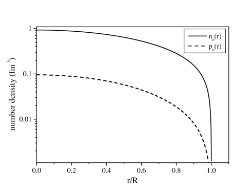
FIG. 2.: The neutron and proton number densities as functions of $r$ for our model star.

This figure illustrates two important things. First of all it is easy to see that we have chosen our parameters in such a way that the proton fraction at the centre of the star is roughly 10%. Secondly, it should be noted that the proton and neutron densities vanish at the same value of $r$. In other words, the surface of the star corresponds to $n_{\rm o}(R)=p_{\rm o}(R)=0$. This is, in fact, a consequence of our choice to enforce chemical equilibrium throughout the star. It obviously means that we are not at this point considering the effects of regions of the star that extend beyond the superfluid: the low-density crust region and the ocean expected to cover the neutron star’s surface. To work with a simplified stellar model is natural at this point, but it is worth pointing out that a formalism for relativistic solid crusts was developed by Carter and Quintana [37] a long time ago. A potentially very interesting extension of the present work concerns the matching of our equations, representing the superfluid core, to a slow-rotation version of the equations of Priou [38], describing the dynamics of solid crusts.

B The Frame-Dragging

Once the background configuration has been determined, the frame-dragging $\omega$ can be calculated from (80). This calculation is standard, but it is notable that the two-fluid results differ from those of Hartle in that a single integration does not suffice to determine the frame-dragging at all rates of rotation. This is simply because the integration of (80) requires the central value of $\tilde{L}_{n}$ as well as both the neutron and the proton rotation rates. In practice, we solve a rescaled version of (80) such that we determine $\hat{L}_{n}=\tilde{L}_{n}/\Omega_{p}$ given $\hat{L}_{n}(0)$ and the relative rotation rate $\Omega_{n}/\Omega_{p}$. This then determines the frame-dragging for all $\Omega_{p}$ with a fixed relative rotation. It is natural to scale the variables with the rotation rate of the protons rather than that of the neutrons since, as we discussed in the Introduction, one would expect the charged components in a neutron star core to be electromagnetically coupled to the nuclei in the crust. This locks the two components (which make up our “proton” fluid) together on a very short timescale. Meanwhile the superfluid neutrons may rotate differently. Furthermore, as will become clear in Section V, there may be situations where one would need to allow the neutrons to rotate with $\Omega_{n}\neq$ constant.

The solution to the frame-dragging equation (80) is to be such that the interior matches smoothly onto the known vacuum solution (96). This means that we must have

$$\tilde{L}_{n}(R)=-\Omega_{n}+{2J\over R^{3}}\ .$$ (114)

We can easily see that $\tilde{L}_{n}$ and its derivative are smooth provided that we have

$$\tilde{L}_{n}(R)=-\Omega_{n}-{R\over 3}\left.{d\tilde{L}_{n}\over dr}\right|_{r=R}\ .$$ (115)

Once we find a value for $\tilde{L}_{n}(0)$ such that (115) is satisfied, we have an acceptable solution to the problem, and we can determine the angular momentum of the configuration from (114).

Having solved the frame-dragging equation for our model star we find (not very surprisingly) that the result differs very little from the standard one-fluid result as long as the relative rotation of the neutrons and the protons is not too extreme. One typically finds that the frame dragging is a smooth function that decreases monotonically from the centre of the star towards the surface. A sample of results are shown in figure 3.

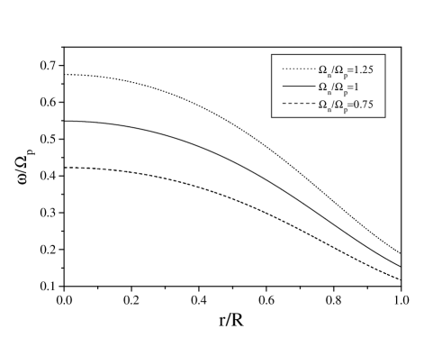
FIG. 3.: Typical results for the frame-dragging $\omega$ for superfluid stars in which the neutrons and the protons rotate at slightly different rates.

Even though the outcome may be of limited physical significance it is interesting to consider more extreme situations, such as ones where the neutrons are rapidly counter-rotating relative to the protons. An example of such a case is shown in figure 4. Here the neutrons rotate backwards with respect to the protons in such a way that $\Omega_{n}=-0.08\Omega_{p}$. This example shows that the two-fluid system allows models where the frame-dragging no longer changes monotonically from the centre to the surface of the star. In the particular case shown in figure 4 the forward rotation of the protons (which make up roughly 10% of the total number density at the centre, cf. figure 2) counteract the frame dragging induced by the neutrons in the central parts of the star. Meanwhile, the backwards rotation of the neutrons dominate the frame-dragging in the surface region.

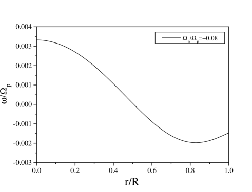
FIG. 4.: The frame dragging in an extreme (rather unphysical) situation where the neutrons and the protons counterrotate in such a way that the net frame dragging is “backwards” at the surface of the star but “forwards” in the central parts.

C The $l=0$ Results

Let us now turn to the next phase of the problem, namely the $l=0$ equations at the ${\cal O}(\Omega^{2})$ level. Thus we consider Eqns. (62), (72), (86) and (92). This corresponds to five equations for $\xi_{0}$, $\eta_{0}$, $\Phi_{0}$, $h_{0}$ and $v_{0}$. We also need to determine the two integration constants $\gamma_{n}$ and $\gamma_{p}$. In practice we proceed as follows: First we introduce a new variable

$$m_{0}=re^{-\lambda}v_{0}\ .$$ (116)

Then we implement the boundary conditions at the centre of the star by requiring that $m_{0}(0)=\xi_{0}(0)=0$ and $h_{0}(0)=\mbox{ constant}$. The first two correspond to spacetime being locally flat at the centre and the requirement that our new coordinate system has the same origin as the spherical coordinates used to describe the non-rotating model. It is also worth noticing that the condition $\xi_{0}(0)=0$ leads to the central energy density of our rotating star necessarily being equal to $-\Lambda_{\rm o}(0)$, i.e. the central density of the non-rotating star. This is true also for the single fluid slow-rotation approximation, cf. [30].

However, in the superfluid case we have an extra degree of freedom. It is not sufficient to provide the total energy density at the centre, we need to also provide either $\eta_{0}(0)$ or $\Phi_{0}(0)$. These represent the change in the neutron and proton central density, respectively. The fact that we have $\xi_{0}(0)=0$ relates these two parameters and we must have

$$\left.\left(\mu_{\rm o}n_{\rm o}\eta_{0}\right)\right|_{r=0}+\left.\left(\chi_{\rm o}p_{\rm o}\Phi_{0}\right)\right|_{r=0}=0\ .$$ (117)

In other words, we only need to provide $\eta_{0}(0)$ (say). In the following we will typically assume that $\eta_{0}(0)=\Phi_{0}(0)=0$, i.e. that the central proton to neutron ratio remains unchanged in the rotating star. However, this choice is made for convenience and there are other options that may be physically more relevant. We discuss such possibilities in section V, but all results presented in this section pertain to the case when $\eta(0)=\Phi_{0}(0)=0$.

Given the data at the centre of the star we can easily determine $\gamma_{n}$ and $\gamma_{p}$ from (72). This leads to

$$\gamma_{n} = h_{0}(0)+\left.\left({\mu_{\rm o}\left.{{\cal A}_{0}^{0}}\right|_{\rm o}-\chi_{\rm o}\left.{{\cal B}_{0}^{0}}\right|_{\rm o}\over\mu_{\rm o}^{2}}p_{\rm o}\Phi_{0}\right)\right|_{r=0},$$ (118)

$$\gamma_{p} = h_{0}(0)+\left.\left({\mu_{\rm o}\left.{{\cal C}_{0}^{0}}\right|_{\rm o}-\chi_{\rm o}\left.{{\cal A}_{0}^{0}}\right|_{\rm o}\over\mu_{\rm o}\chi_{\rm o}}p_{\rm o}\Phi_{0}\right)\right|_{r=0}\ .$$ (120)

Now we are set to solve the various $l=0$ equations. We do this by integrating (86) and (92) using a standard fourth order Runge-Kutta scheme. After each integration step we determine the relevant values for $\xi_{0}$, $\eta_{0}$ and $\Phi_{0}$ by solving the algebraic equations (62) and (72). At the surface of the star the solutions for $h_{0}$ and $m_{0}$ must be matched to the vacuum solutions given in section IIIC. Once we find a value for $h_{0}(0)$ such that both $h_{0}$ and its derivative match the vacuum result we have our desired solution to the $l=0$ problem. The matching at the surface also determines $\delta M$, the rotationally induced change in inertial mass of the star. For the particular stellar model shown in figure 2 and the case when the two fluids are corotating we find that

$$\delta M=0.091\left({\nu_{p}\over 1~{}\mbox{kHz}}\right)^{2}M_{\odot}\ ,$$

where $\nu_{p}=\Omega_{p}/2\pi$ is the rotation rate of the protons. As we will discuss in Section VB the mass-shedding limit for this star corresponds to $\nu_{p}=1630$ Hz, which means that rotation may increase the inertial mass of the star by up to roughly 17 %. The rotationally induced increase in mass for a sequence of models is illustrated in figure 5. We compare the mass of each non-rotating star to the maximum mass (which is reached when the star spins at the Kepler limit (see section V for a discussion). In the figure we indicate (by an arrow) the rotating analogues of the model star from figure 2 that we construct within the slow-rotation approximation. We also show more “realistic” sequences based on conserving the total baryon number (see section V). In addition, the figure shows that, just as for single-fluid stars, there will be a family of supramassive stars that have no stable non-rotating counterpart [36].

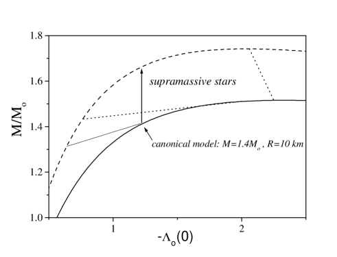
FIG. 5.: We compare the mass of the non-rotating star (solid line) to its maximum value in the rotating case (which is reached when the star spins at the Kepler limit, dashed line) for a sequence of stars parameterized by the central energy density $-\Lambda_{\rm o}(0)$. The vertical arrow indicates rotating configurations with the same central energy density as the canonical model shown in figure 2. The dotted line starting at the base of the arrow shows a more “realistic” sequence of rotating stars constructed by conserving the total baryon number. We also show a similar sequence corresponding to the maximum mass non-rotating star (upper dotted line). Above this latter line, the various stars have no stable non-rotating counterpart, they are the so-called supramassive stars.

Another illustration of the effects that rotation has on the inertial mass of the star is shown in figure 6. Here we show how the total mass for a star rotating at the Kepler limit depends on the relative rotation between the neutrons and the protons. The particular results are for our canonical stellar model from figure 2, and the behaviour is easily understood if we compare the results for the mass to the Kepler frequency results in figure 12.

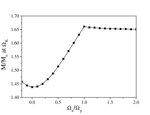
FIG. 6.: An illustration of how the total gravitational mass for a star rotating at the Kepler limit depends on the relative rotation between the neutrons and the protons. These particular results are for our canonical stellar model.

The obtained solution for $h_{0}$ is illustrated in Figure 7. The variables $\xi_{0}$, $\eta_{0}$ and $\Phi_{0}$ that are solved for algebraically are shown in figures 8-10. In these figures it is worth noticing that the rotational correction to the neutron number density $\eta_{0}$ diverges at the surface. One can easily show that such a divergence will be present whenever the index of the corresponding polytrope (here $\beta_{n}$) is larger than 2. It should be pointed out, however, that this does not affect the determination of any physical parameters such as the total mass or the corresponding baryon number. Finally, we note that the function $m_{0}$ increases monotonically from the centre to the surface. Hence, we do not illustrate it here.

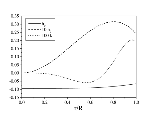
FIG. 7.: The metric functions $h_{0}$, $h_{2}$ and $\tilde{k}$ for our model star and the case when the superfluid neutrons corotate with the protons ($\Omega_{n}=\Omega_{p}$). This particular data corresponds to the protons rotating at $\nu_{p}=1$ kHz.

D The $l=2$ Results

The final step in constructing a slowly rotating superfluid star consists of solving the $l=2$ equations (63), (79), (82), 83) and (95). These equations determine $\xi_{2}$, $\eta_{2}$, $\Phi_{2}$, $h_{2}$, $v_{2}$ and $k_{2}$. Equation (89) contains no new information and we will not use it here.

The strategy for solving these equations is similar to that we adopted for the $l=0$ problem. In the $l=2$ case it is, however, useful to rewrite the equations somewhat. We note that once a solution to the differential equations (83) and (95) is obtained, all other variables follow algebraically. As Hartle points out [30], it is convenient to introduce a new variable $\tilde{k}=k_{2}+h_{2}$. This definition and some straightforward manipulations lead to two coupled equations for $\tilde{k}$ and $h_{2}$. These can be written

$$\tilde{k}^{\prime} + \nu^{\prime}h_{2}={r^{3}\over e^{\nu}}\left(2+r\nu^{\prime}\right)\left\{{1\over 12e^{\lambda}}\left({d\tilde{L}_{n}\over dr}\right)^{2}+{4\pi\over 3}\left[(\Psi_{0}-\Lambda_{0})\tilde{L}_{n}^{2}+\chi_{0}p_{0}(\tilde{L}_{n}+\tilde{L}_{p})(\Omega_{n}-\Omega_{p})-A_{0}n_{0}p_{0}(\Omega_{n}-\Omega_{p})^{2}\right]\right\}\ ,$$ (121)

$$h_{2}^{\prime} + \left\{\nu^{\prime}+{1\over\nu^{\prime}}\left[{2e^{\lambda}-2\over r^{2}}+8\pi e^{\lambda}(\Lambda_{0}-\Psi_{0})\right]\right\}h_{2}+{4e^{\lambda}\over r^{2}\nu^{\prime}}\tilde{k}=$$ (122)

$$= {r^{2}\over 12e^{\nu}\nu^{\prime}}\left\{\left(r^{2}e^{-\lambda}(\nu^{\prime})^{2}-2\right)\left({d\tilde{L}_{n}\over dr}\right)^{2}+16\pi r^{2}(\nu^{\prime})^{2}(\Psi_{0}-\Lambda_{0})\tilde{L}_{n}^{2}\right.$$ (123)

$$+ \left.32\pi e^{\lambda}(\mu_{0}n_{0}\tilde{L}_{n}^{2}+\chi_{0}p_{0}\tilde{L}_{p}^{2})+16\pi\chi_{0}p_{0}r^{2}(\nu^{\prime})^{2}(\Omega_{n}-\Omega_{p})(\tilde{L}_{n}+\tilde{L}_{p})-16\pi n_{0}p_{0}A_{0}\left(2e^{\lambda}+r^{2}(\nu^{\prime})^{2}\right)(\Omega_{n}-\Omega_{p})^{2}\right\}\ .$$ (124)

By analyzing these equations for small values of $r$ we find that in order to have a regular solution we must require that $h_{2}=c_{1}r^{2}$ and $\tilde{k}=c_{2}r^{4}$ near the centre of the star. A series expansion of (124) then reveals that the two constants $c_{1}$ and $c_{2}$ should be related according to

$$c_{2}+2\pi\left(\Psi_{0}-{1\over 3}\Lambda_{0}\right)c_{1}=$$ (125)

$${2\pi\over 3e^{\nu}}\left[2(\Psi_{0}-\Lambda_{0})\tilde{L}_{n}^{2}-n_{0}p_{0}A_{0}(\Omega_{n}-\Omega_{p})^{2}-2\chi_{0}p_{0}(\Omega_{n}-\Omega_{p})(\tilde{L}_{n}+\tilde{L}_{p})-(\mu_{0}n_{0}\tilde{L}_{n}^{2}+\chi_{0}p_{0}\tilde{L}_{p}^{2})\right]\ .$$ (126)

Furthermore, since we know that $\xi_{2}\to 0$ as $r\to 0$ we can deduce from (63) and 79) that we must have $\eta_{2}=\Phi_{2}=0$ at the centre of the star.

Schematically, we solve the $l=2$ equations as follows: First we find a solution to (121) and (124) that matches smoothly onto the vacuum solution at the surface of the star (cf. Section IIIC). We do this by finding a particular solution to the full problem and adding to it a multiple of the solution to the corresponding homogeneous problem, where the right hand sides of (121) and (124) are set equal to zero and the two constants are related by

$$c_{2}+2\pi\left(\Psi_{0}-{1\over 3}\Lambda_{0}\right)c_{1}=0\ .$$ (127)

The desired solution for $[\tilde{k},h_{2}]$ is then the linear combination that gives the vacuum relation between these two variables at the surface. Having determined the appropriate linear combination of the interior functions (as well as the constant $A$ in the equations in Section IIIC) we can readily reconstruct the full solution, and in addition solve (63) and (79) for $\xi_{2}$, $\eta_{2}$ and $\Phi_{2}$ after each integration step. This then completes the construction of a slowly rotating superfluid stellar model. Typical results for our model star are shown in figures 7-10.

Once we have solved all the $l=2$ equations we can work out the rotationally induced change in the shape of the star, i.e. the centrifugal flattening. This effect is conveniently expressed in terms of the ratio between the polar and equatorial radii, $R_{p}$ and $R_{e}$ respectively. Within the slow-rotation approximation this leads to

$${R_{p}\over R_{e}}\approx 1+{3\xi_{2}(R)\over 2R}$$ (128)

and for our model star (with $\eta_{0}(0)=0$ and $\Omega_{n}=\Omega_{p}$) we get

$${R_{p}\over R_{e}}\approx 1-0.113\left({\nu_{p}\over 1~{}\mbox{kHz}}\right)^{2}\ .$$ (129)

Thus, we find $R_{p}/R_{e}\approx 0.7$ for a star spinning at the mass-shedding limit.

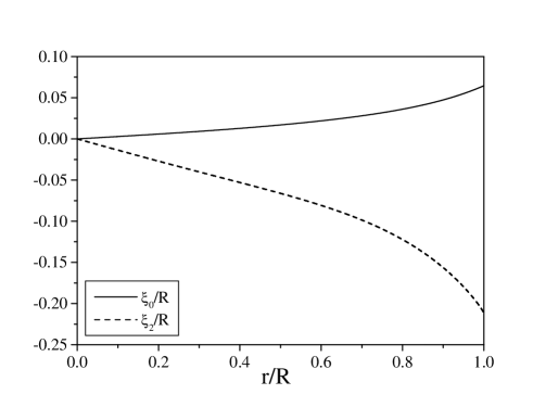
FIG. 8.: The functions $\xi_{0}$ and $\xi_{2}$ for our model star and the case when the superfluid neutrons corotate with the protons ($\Omega_{n}=\Omega_{p}$).This particular data corresponds to the protons rotating at $\nu_{p}=1$ kHz.

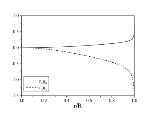
FIG. 9.: The rotationally induced changes in the neutron number density, $\eta_{0}$ and $\eta_{2}$, for our model star and the case when the superfluid neutrons corotate with the protons ($\Omega_{n}=\Omega_{p}$).This particular data corresponds to the protons rotating at $\nu_{p}=1$ kHz.

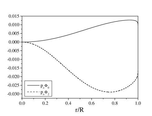
FIG. 10.: The rotationally induced change in the proton number density, $\Phi_{0}$ and $\Phi_{2}$, for our model star and the case when the superfluid neutrons corotate with the protons ($\Omega_{n}=\Omega_{p}$). This particular data corresponds to the protons rotating at $\nu_{p}=1$ kHz.

Once we have solved the $l=2$ equations and determined the value of $A$ we can calculate the quadrupole moment from (108). In doing this it is useful to construct two dimensionless quantities

$$q=\left({c^{2}\over GM}\right){Q\over M}\quad,\mbox{ and }\quad\chi={c\over G}{J\over M^{2}}\ .$$ (130)

Once we do this, we can compare our results to those of Laarrakers and Poisson [35] who study the quadrupole moment of rapidly rotating single fluid stars for realistic equations of state. In figure 11 we compare our results to theirs by showing the dependence of the ratio $q/\chi^{2}$ on the mass of the star. Clearly, the present results for the quadrupole moment are reasonable. It should also be noted that one would have $q/\chi^{2}=-1$ for a Kerr black hole. Thus figure 11 emphasizes the well-know fact that rotating neutron stars have a multipole structure that is radically different from that of the Kerr spacetime.

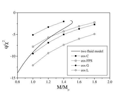
FIG. 11.: Our results for the quadrupole moment (in terms of the ratio $q/\chi^{2}$, see the main text for definitions) as a function of the stellar mass are compared to numerical results obtained for rapidly rotating relativistic stars using realistic supranuclear equations of state.

V Sequences of stars

Given the machinery we have developed in the previous sections we are set to ask physically relevant questions. Ideally, we would like to be able to construct a sequence of rotating models that can meaningfully be said to represent the same non-rotating star. Given that we can allow the neutrons and the protons to rotate differently, and also adjust the relative central densities, the construction of such a sequence of models is non-trivial. However, a natural starting point may be to first determine the maximum allowed rate of rotation. Then we will discuss conservation of the total integrated neutron and proton numbers along a sequence of rotating stars. To impose this requirement corresponds to determining the total baryon numbers for the neutrons and the protons and then finding models such that these quantities are held constant as the spin-rate increases. Finally, we will turn to issues regarding chemical equilibrium.

A The Kepler limit

The maximum spin-rate of a stationary configuration corresponds to the so-called Kepler frequency. It is determined as the rotation rate where mass-shedding sets in at the equator. The corresponding frequency can be calculated by requiring that the rotation rate of the fluid be equal to the frequency of a particle orbiting the star on an equatorial geodesic. The determination of the Kepler frequency for our slowly rotating stars is relatively straightforward. After all, the main part of the calculation involves the rotation frequency of an orbiting particle, and as far as the exterior vacuum is concerned, the fact that we are dealing with the rotation of two coupled fluids is irrelevant. The only subtlety of the two-fluid problem involves the fact that we can allow the protons and neutrons to rotate at different rates. Clearly, the Kepler limit will be determined by whichever fluid is rotating the fastest at the surface. In other words, we simply take $\Omega_{K}=\mbox{max }(\Omega_{n},\Omega_{p})$ in the following. It should, of course, be noted that the situation is simpler for more realistic neutron star models. Then the Kepler frequency will be determined from the rotation rate of the crust.

For a rapidly rotating star the Kepler frequency $\Omega_{K}$ can be determined from (cf. Friedman, Ipser and Parker[39])

$$\Omega_{K}={Nv\over\sqrt{K}}+\omega$$ (131)

where the metric variables are defined by (8) and

$$v={K^{3/2}\omega^{\prime}\over NK^{\prime}}+\sqrt{{2KN^{\prime}\over NK^{\prime}}+\left({K^{3/2}\omega^{\prime}\over NK^{\prime}}\right)^{2}}$$ (132)

is the orbital velocity according to a zero-angular momentum observer at the equator (where all quantities should be evaluated). Here primes denote derivatives with respect to $\tilde{r}$. In order to be consistent, we expand this equation keeping only terms up to (and including) order $\Omega^{2}$. Then we get

$$\Omega_{K}\approx{e^{\nu/2}\over\tilde{r}}\sqrt{{\tilde{r}\nu^{\prime}\over 2}}+\omega+{\tilde{r}\omega^{\prime}\over 2}+e^{\nu/2}\sqrt{{\nu^{\prime}\over 2\tilde{r}}}\left[h-k+{h^{\prime}\over\nu^{\prime}}-{\tilde{r}k^{\prime}\over 2}+{\tilde{r}^{3}(\omega^{\prime})^{2}\over 4\nu^{\prime}e^{\nu}}\right]+O(\Omega^{3})\ .$$ (133)

The next step corresponds to using the vacuum expressions for the various slow-rotation quantities, and also doing the coordinate transformation $\tilde{r}\to r$. Luckily, the latter affects only the first term in (133). After some algebra we arrive at our final expression

$$\Omega_{K}=\sqrt{M\over R^{3}}-{\hat{J}\Omega_{p}\over R^{3}}+\sqrt{M\over R}\left\{{\delta\hat{M}\over 2M}+{(R+3M)(3R-2M)\over 4R^{4}M^{2}}\hat{J}^{2}-{3\over 4}{2\hat{\xi}_{0}+\hat{\xi}_{2}\over R^{2}}+\alpha\hat{A}\right\}\Omega_{p}^{2}$$ (134)

where we have made the scaling with $\Omega_{p}$ explicit by introducing $J=\hat{J}\Omega_{p}$ etc. We have also defined

$$\alpha={3(R^{3}-2M^{3})\over 4M^{3}}\log\left(1-{2M\over R}\right)+{3R^{4}-3R^{3}M-2R^{2}M^{2}-8RM^{3}+6M^{4}\over 2RM^{2}(R-2M)}\ .$$ (135)

Here it should be noted that, at the $\Omega^{2}$ level the Kepler limit depends explicitly on the rotationally induced change in mass, the centrifugal flattening as well as the change in quadrupole moment (through $A$).

In order to determine the Kepler limit for our rotating superfluid models we simply have to solve the above quadratic for $\Omega_{p}$. This then tells us the maximum allowed spin-rate for the protons at any given central energy density and relative (constant) rotation rate $\Omega_{n}/\Omega_{p}$. Typical results of this exercise are shown in figure 12. In this figure we show how the Kepler frequency is affected by changes in the relative rotation rate $\Omega_{n}/\Omega_{p}$. The results can be understood in the following way: For $\Omega_{n}/\Omega_{p}=1$ the two fluids rotate together so we have a fairly standard result. For the model star from figure 2 we find that the Kepler frequency is $\Omega_{K}=\Omega_{p}=\Omega_{n}\approx 1.02\times 10^{4}$ rad/s or $\nu_{K}\approx 1630$ Hz. When we compare this to the relation (30) we see that it is not an unreasonable result, although it is roughly 10% higher than the empirical estimate for the relevant mass and radius. Figure 12 also provides information regarding the effects of differential rotation. First of all it is clear that when $\Omega_{n}>\Omega_{p}$ the Kepler rate is determined by the neutrons. Given that the neutrons make up more than 90% of the material in the star it is not too surprising that the result for $\Omega_{K}$ changes very little as we increase $\Omega_{n}$ beyond $\Omega_{p}$. Basically, the star rotates like a single fluid star with a dynamically small proton component. The opposite case, when $\Omega_{n}<\Omega_{p}$, is more interesting. Then we see that the maximum allowed spin rate for the protons increases as $\Omega_{n}$ decreases. We can deduce that this is reasonable from (134): As we decrease the rotation rate of the neutrons the various $\Omega_{p}^{2}$ terms all decrease (again, because the neutrons make up most of the star and so have a dominant effect). Thus it follows naturally that the orbital frequency of a particle at the equator will approach the non-rotating star case. In other words, it increases which leads to the maximum allowed rotation of the protons increasing as well.

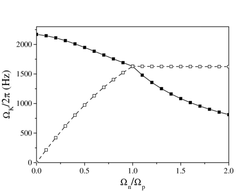
FIG. 12.: The Kepler limit $\Omega_{K}$ is shown as a function of the relative rotation rate $\Omega_{n}/\Omega_{p}$ for our model star. The filled squares show the maximum allowed rotation rate for the protons ($\Omega_{p}$), while the open squares show the corresponding neutron spin rate ($\Omega_{n}$). The Kepler frequency simply corresponds to the largest of the two.

B The baryon numbers and angular momenta

We want to determine the conserved neutron number $N_{n}$, the conserved proton number $N_{p}$, and then define the total baryon mass $M_{B}$ as

$$M_{B}=m_{n}N_{n}+m_{p}N_{p}\ ,$$ (136)

where $m_{n}$ is the neutron mass and $m_{p}$ is the proton mass. One of the assumptions behind the general relativistic superfluid formalism implemented here is that the neutrons and the protons are independently conserved. Thus the formulas for the conserved particle numbers can be obtained by integrating the conservation rules (14) over a bounded region of spacetime, and then using the generalized Stokes Theorem to reduce the spacetime volume integral to three-dimensional integration over the boundary. The bounded spacetime region is the four-dimensional volume contained between the two spacelike slices given by $t=t_{1}$ and $t=t_{2}$ where $t_{1}$ and $t_{2}$ are constants. The timelike boundary of this volume is the union of each sphere at infinity that exists on each $t=$ constant spacelike slice. Because the matter is assumed to have compact support, there will be no contributions to the baryon mass formula from the timelike boundary. All that remains are two integrals, one on the $t=t_{1}$ and another on the $t=t_{2}$ hypersurface, that add to zero. The $t=t_{2}$ integral, say, then yields the conserved particle number.

The conserved neutron particle number is thus found to be

$$N_{n}=-\int_{t=const}n^{\mu}\eta_{\mu}\sqrt{\gamma}{\rm d}^{3}x\ ,$$ (137)

where $\gamma={\rm det}\gamma_{ij}$ and $\gamma_{ij}$ is the intrinsic metric of the $t=$ constant hypersurface, i.e. the metric is assumed to have a $3+1$ decomposition of the form

$${\rm d}s^{2}=-\left(N^{2}-\gamma_{ij}N^{i}N^{j}\right){\rm d}t^{2}+2\gamma_{ij}N^{j}{\rm d}x^{i}{\rm d}t+\gamma_{ij}{\rm d}x^{i}{\rm d}x^{j}\ ,$$ (138)

and the (future-directed) normal to the $t=$ constant hypersurfaces, to be denoted $\eta^{\mu}$, is given by $\eta_{\mu}=(-N,0,0,0)$. The formula for $N_{p}$ is identical except that $n^{\mu}$ is replaced with $p^{\mu}$. One important point to keep in mind is that the surface of the star (which will be non-spherical in general) is given by $r=$ constant, cf. Figure 1. In terms of the metric and particle number density currents developed for the slow rotation formalism it is found that

$$N_{n}=4\pi\int_{0}^{R}{\rm d}rr^{2}e^{\lambda/2}n_{\rm o}\left(1+\eta_{0}+v_{0}+\left[{\lambda^{\prime}\over 2}+{2\over r}\right]\xi_{0}+{2r^{2}\over 3e^{\nu}}\tilde{L}^{2}_{n}\right)\ ,$$ (139)

$$N_{p}=4\pi\int_{0}^{R}{\rm d}rr^{2}e^{\lambda/2}p_{\rm o}\left(1+\Phi_{0}+v_{0}+\left[{\lambda^{\prime}\over 2}+{2\over r}\right]\xi_{0}+{2r^{2}\over 3e^{\nu}}\tilde{L}^{2}_{p}\right)\ .$$ (140)

As an illustration we note that in the case of the model in Figure 2, and $\Omega_{n}=\Omega_{p}$, the two baryon masses are

$$M_{Bn}/M_{\odot} \approx 1.46+0.13\left({\nu_{p}\over 1~{}\mbox{kHz}}\right)^{2}$$

$$M_{Bp}/M_{\odot} \approx 0.11+0.027\left({\nu_{p}\over 1~{}\mbox{kHz}}\right)^{2}\ .$$

In the standard single fluid case one would typically identify a distinct sequence of rotating models as representing “the same” star by requiring that the total baryon rest mass be conserved. In our present problem, the fact that we are dealing with two distinct fluids provides additional complications. Provided that the star spins up (or down) rapidly enough compared to the nuclear reactions that convert neutrons to protons (and vice versa) it would be reasonable to conserve the total integrated neutron and proton neutron numbers individually. However, the spin-evolution of a neutron star typically proceeds slowly. Furthermore, as discussed by Reisenegger [40], one would expect a certain amount of conversion between the two fluids as the star spins down simply because of the change in shape of the constant density surfaces. In other words, in the two fluid case it is not obvious how to construct an “astrophysical sequence” of rotating stars based on the two baryon masses.

Anyway, let us suppose that we want to demand that the individual integrated baryon numbers are conserved as we spin the star up. From the above results we see that this corresponds to

$$\delta N_{n}=\int_{0}^{R}{\rm d}rr^{2}e^{\lambda/2}n_{\rm o}\left(\eta_{0}+v_{0}+\left[{\lambda^{\prime}\over 2}+{2\over r}\right]\xi_{0}+{2r^{2}\over 3e^{\nu}}\tilde{L}^{2}_{n}\right)=0\ ,$$ (141)

and

$$\delta N_{p}=\int_{0}^{R}{\rm d}rr^{2}e^{\lambda/2}p_{\rm o}\left(\Phi_{0}+v_{0}+\left[{\lambda^{\prime}\over 2}+{2\over r}\right]\xi_{0}+{2r^{2}\over 3e^{\nu}}\tilde{L}^{2}_{p}\right)=0\ .$$ (142)

Let us consider the (by now familiar) stellar model from figure 2. According to the result above we then have

$$M_{B}=M_{Bn}+M_{Bp}=(1.46+0.11)M_{\odot}=1.57M_{\odot}\ ,$$

in the rotating case. First of all we find that the two baryon masses are not individually conserved for the star that has the same total $M_{B}$ at the Kepler limit. At least not if we take $\eta_{0}(0)=0$ and $\Omega_{n}/\Omega_{p}=1$. For this case we find

$$M_{Bn}=1.48M_{\odot}\ ,\qquad\mbox{ and }\qquad M_{Bp}=0.09M_{\odot}\ .$$

However, we have the freedom to choose our parameters differently and we find that we can conserve both baryon masses by adjusting either $\eta_{0}(0)$ or $\Omega_{n}/\Omega_{p}$ (or, indeed, both of them). For example, we find that both $M_{Bn}$ and $M_{Bp}$ are the same as in the non-rotating star if we take

$$\eta_{0}(0) = -4\times 10^{-2}\left({\nu_{p}\over 1~{}\mbox{kHz}}\right)^{2}\quad\mbox{ and }\quad\Omega_{n}/\Omega_{p}=1\ ,$$

$$\eta_{0}(0) = 0\quad\mbox{ and }\quad\Omega_{n}/\Omega_{p}=0.75\ .$$

This is an interesting illustration of the subtleties involved in constructing rotating superfluid neutron star configurations.

Furthermore, the fact that the slow-rotation calculation requires, once a non-rotating star is given, the specification of both $\Omega_{n}/\Omega_{p}$ and $\eta_{0}(0)$ leads us to ask an intriguing question: We have two seemingly free parameters and two equations, (141) and (142). Is it possible to specify these constants in such a way that the two baryon numbers are conserved even though we keep the central density of the star fixed? In the standard one-fluid case this would certainly not be possibly. As the spin of the star increases the centrifugal flattening will necessarily lead to decrease in the central density (for a star with a fixed number of baryons). Is it possible that two-fluid models offer a somewhat counter-intuitive alternative? That is, is it possible to carefully redistribute the neutrons and the protons (in such a way that the central energy density remains unchanged), and spin the star up without causing the familiar increase in baryon mass? For our particular model equation of state we find a negative answer to this question, cf. Figure 13. However, it is an intriguing possibility and we cannot at this point argue why it could not happen for some other, perhaps more realistic, equation of state.

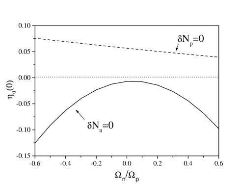
FIG. 13.: Curves corresponding to conservation of the total number of neutrons ($\delta N_{n}=0$) and the total number of protons ($\delta N_{p}=0$) are shown as functions of the two free parameters $\eta_{0}(0)$ and $\Omega_{n}/\Omega_{p}$. (The data corresponds to the case $\nu_{p}=$1 KHz.) A point of intersection would correspond to a rotating model which conserves both the individual baryon masses from the non-rotating star. As is clear from the data, such models cannot be constructed for our model equation of state (which agrees with the standard result from the one-fluid case). This does not, however, rule out this possibility for other equations of state.

Using the above set-up for the bounded spacetime region, we can also make meaningful definitions for the individual neutron and proton total angular momenta, to be denoted $J_{n}$ and $J_{p}$ respectively. Langlois et al [8] demonstrate that such an unambiguous separation can be made if the hypersurface over which the integrals are being performed is invariant under the axisymmetry action. In the present context this means that the scalar product of the spacelike Killing vector $\phi^{\mu}$ with the normal to our hypersurface $\eta^{\mu}$ must be zero. Indeed, it is trivial to verify that we have $\phi^{\nu}\eta_{\nu}=0$. Now, according to Langlois et al, the two angular momenta are given by

$$J_{n}=-\int_{t=const}\left(\phi^{\nu}\mu_{\nu}\right)n^{\mu}\eta_{\mu}\sqrt{\gamma}{\rm d}^{3}x\quad,\quad J_{p}=-\int_{t=const}\left(\phi^{\nu}\chi_{\nu}\right)p^{\mu}\eta_{\mu}\sqrt{\gamma}{\rm d}^{3}x\ .$$ (143)

In terms of the slow-rotation approximation, we find for the neutron total angular momentum

$$J_{n}=-{8\pi\over 3}\int_{0}^{R}{\rm d}rr^{4}e^{(\lambda-\nu)/2}\left[\mu_{\rm o}n_{\rm o}\tilde{L}_{n}+{\cal A}_{\rm o}n_{\rm o}p_{\rm o}\left(\Omega_{n}-\Omega_{p}\right)\right]$$ (144)

and the very similar form

$$J_{p}=-{8\pi\over 3}\int_{0}^{R}{\rm d}rr^{4}e^{(\lambda-\nu)/2}\left[\chi_{\rm o}p_{\rm o}\tilde{L}_{p}+{\cal A}_{\rm o}n_{\rm o}p_{\rm o}\left(\Omega_{p}-\Omega_{n}\right)\right]$$ (145)

for the proton total angular momentum. It is easy to verify that

$$J=J_{n}+J_{p}\ ,$$ (146)

where $J$ is the total angular momentum found earlier by matching to the exterior vacuum solution of Hartle.

C Chemical Equilibrium

So far we have not imposed chemical equilibrium in our rotating stars (although it was assumed for the non-rotating background model). This is quite reasonable since one can easily think of situations where the two fluids are temporarly rotation “out of sync” following for example a glitch. As we argued in the Introduction it will then likely take the various relevant mechanisms many hundreds of dynamical timescales to again lock the two components together. And it may take much longer for chemical equilibrium to be restored given that this happens on the characteristic timescale of the various nuclear reactions. Anyway, before we conclude this paper it is obviously meaningful to address the issue of chemical equilibrium. Intuitively, one might expect that one can only have equilibrium when the neutrons and the protons corotate. The argument for this is simple: If the two species rotate at different rates we must work in one of the two frames (the nuclear reactions that re-establish equilibrium depend on the local physics), and the result will depend on which frame we choose. In the frame rotating with the neutrons the proton chemical potential will have an additional kinematic piece. This is also true for the neutron chemical potential in the frame that corotates with the protons. In other words, it would seem possible to have equilibrium only if the two fluids corotate.

This is, of course, just a hand-waving argument and we need to support it mathematically. Let us first return to a situation where $\Omega_{n}$ and $\Omega_{p}$ are not assumed to be constant. Langlois et al [8] have shown that chemical equilibrium is imposed on the system via the condition

$$p^{\nu}\left(\mu_{\nu}-\chi_{\nu}\right)=0\ .$$ (147)

Using the results from Section II we immediately find that this corresponds to

$$t^{\nu}\mu_{\nu}+\Omega_{p}\phi^{\nu}\mu_{\nu}=t^{\nu}\chi_{\nu}+\Omega_{p}\phi^{\nu}\chi_{\nu}\ .$$ (148)

Let us now assume, again, that $\Omega_{p}$ is constant. As we have already argued in Section IV, this is likely to be the case in most astrophysical neutron stars. The Euler equation for the protons (15) then implies that the right-hand-side of the above condition is a constant. Thus we have

$$t^{\nu}\chi_{\nu}+\Omega_{p}\phi^{\nu}\chi_{\nu}=\mbox{ constant}\ .$$ (149)

Obviously, this also implies that

$$t^{\nu}\mu_{\nu}+\Omega_{p}\phi^{\nu}\mu_{\nu}=\mbox{ constant}\ .$$ (150)

We solve for $t^{\nu}\mu_{\nu}$ and then put the result into the Euler equation for the neutrons. This way we obtain

$$(\Omega_{n}-\Omega_{p})\partial_{\mu}(\phi^{\nu}\mu_{\nu})=0\ .$$ (151)

From this we can conclude the following: If one demands chemical equilibrium, and also assumes that $\Omega_{p}$ is constant (that the protons rotate rigidly), then one of the following two conditions must be true,

$$\Omega_{n}-\Omega_{p}=0\ ,$$ (152)

or

$$\phi^{\nu}\mu_{\nu}=\mbox{ constant}\ .$$ (153)

The first of these is the result that we anticipated, that chemical equilibrium would lead to the two fluids co-rotating. The second condition is a bit more puzzling, and we need to ask whether one can have a physical configuration that satisfies it.

Taking the slow-rotation form for $\mu_{\nu}$ the second condition becomes

$$-r^{2}{\rm sin}^{2}\theta e^{-\nu/2}[{\cal B}_{\rm o}n_{\rm o}(\omega-\Omega_{n})+{\cal A}_{\rm o}p_{\rm o}(\omega-\Omega_{p})]=\mbox{ constant}\ .$$ (154)

From this it is clear that unless the right-hand-side vanishes then $\omega$ and $\Omega_{n}$ are both badly behaved at the origin (as well as at the poles). Thus we can only have a well-behaved solution if

$$\Omega_{n}=[({\cal B}_{\rm o}n_{\rm o}+A_{\rm o}p_{\rm o})/({\cal B}_{\rm o}n_{\rm o})]\omega-[A_{\rm o}p_{\rm o}/{\cal B}_{\rm o}n_{\rm o}]\Omega_{p}\ .$$ (155)

In the special case with no entrainment we have ${\cal A}_{\rm o}=0$, and our condition implies

$$\Omega_{n}=\omega\ .$$ (156)

Hence, we see that the second condition for chemical equilibrium condition links the rotation rate of the superfluid neutrons to the frame-dragging. This means that, in order to satisfy this condition, the neutrons must rotate differentially. At first this possible solution may seem peculiar, but it may in fact make sense if we consider the physical meaning of the frame-dragging. The condition (156) simply says that the neutrons are not rotating with respect to a local zero-angular momentum observer. They are simply dragged along by the rotation of the protons.

From this discussion we conclude that if the two fluids both rotate uniformly and $\Omega_{n}\neq\Omega_{p}$ then one cannot impose chemical equilibrium. When chemical equilibrium is imposed, the two fluids must either corotate, or $\Omega_{n}$ must have differential rotation (and in fact be equal to the frame-dragging $\omega$ when there is no entrainment).

We note that one could, in principle, explore the latter possibility further. We can combine the condition for equilibrium with the frame-dragging equation (80) in an interesting way. First we re-express (80) in terms of $\tilde{L}_{p}$. Then we get

$${1\over r^{4}}\left(r^{4}e^{-(\lambda+\nu)/2}\tilde{L}_{p}^{\prime}\right)^{\prime}-16\pi e^{(\lambda-\nu)/2}\left(\Psi_{\rm o}-\Lambda_{\rm o}\right)\tilde{L}_{p}=16\pi e^{(\lambda-\nu)/2}\mu_{o}n_{o}\left(\Omega_{p}-\Omega_{n}\right)\ .$$ (157)

By making use of (155) we readily rewrite this as

$${1\over r^{4}}\left(r^{4}e^{-(\lambda+\nu)/2}\tilde{L}_{p}^{\prime}\right)^{\prime}-16\pi e^{(\lambda-\nu)/2}\left[\Psi_{\rm o}-\Lambda_{\rm o}+{\mu_{\rm o}\over{\cal B}_{\rm o}}\left({\cal B}_{\rm o}n_{\rm o}+{\cal A}_{\rm o}p_{\rm o}\right)\right]\tilde{L}_{p}=0\ .$$ (158)

This alternative frame-dragging equation now takes the same form as the single-fluid equation derived by Hartle [30] (the difference being in the factor multiplying $\tilde{L}_{p}$). Thus we know that if we were to solve it numerically we would find that $\tilde{L}_{p}$ decreases monotonically from the centre of the star to the surface. In other words, the results would be similar to those shown in figure 3. In view of this we do not show such results here.

VI Conclusions

In this paper we have developed a framework for constructing and analyzing slowly rotating relativistic superfluid neutron stars. The model is based on the standard two-fluid representation for superfluids wherein all the charged components: protons, electrons and lattice nuclei, are considered as a single fluid coexisting with the superfluid neutrons. We have applied the formalism to a simple equation of state for which the two fluids are described by polytropes. We have then studied the effects of rotation on the resultant stars, with particular focus on the effects due to the fact that the two fluids need not rotate together.

The present results provide a framework that opens the door to fully relativistic studies of many important astrophysical problems. We are currently extending this work in two directions. First, we are investigating the effects of entrainment on rotating stellar models. Secondly, we are extending previous studies of quasinormal mode oscillations in relativistic superfluid stars [18] to incorporate the effects of slow rotation. Of particular interest would be a study of the low-frequency inertial modes, following in the footsteps of Lockitch et al. [26]. The calculation of such modes has been brought into sharp focus since the discovery that the r-modes are generically unstable due to the emission of gravitational waves. So far the only study of the r-modes in the superfluid context is the Newtonian work of Lindblom and Mendell [28]. Our plan is to study the same problem within the framework of relativity. This is an issue that demands immediate attention given the possibility that the r-modes may lead to detectable gravitational waves and the fact that a new generation of large scale interferometric detectors will come on-line soon.

VII Appendix I

Here we give the four combinations used in the right-hand-sides of the field equations that determine the four metric coeffcients

$$T^{0}_{0} = \Lambda_{\rm o}-\mu_{\rm o}n_{\rm o}\left(\eta-{r^{2}{\rm sin}^{2}\theta\over e^{\nu}}\Omega_{n}\tilde{L}_{n}\right)-\chi_{\rm o}p_{\rm o}\left(\Phi-{r^{2}{\rm sin}^{2}\theta\over e^{\nu}}\Omega_{p}\tilde{L}_{p}\right)+$$ (161)

$${r^{2}{\rm sin}^{2}\theta\over 2e^{\nu}}{\cal A}_{\rm o}n_{\rm o}p_{\rm o}\left(\Omega_{n}-\Omega_{p}\right)^{2}\ ,$$

$$T^{1}_{1} = \Psi_{\rm o}+n_{\rm o}\left(n_{\rm o}\left.{{\cal B}_{0}^{0}}\right|_{\rm o}+p_{\rm o}\left.{{\cal A}_{0}^{0}}\right|_{\rm o}\right)\eta+p_{\rm o}\left(p_{\rm o}\left.{{\cal C}_{0}^{0}}\right|_{\rm o}+n_{\rm o}\left.{{\cal A}_{0}^{0}}\right|_{\rm o}\right)\Phi+$$ (165)

$${r^{2}{\rm sin}^{2}\theta\over 2e^{\nu}}n_{\rm o}p_{\rm o}\left({\cal A}_{\rm o}+n_{\rm o}\left.{\partial{\cal A}\over\partial n}\right|_{\rm o}+p_{\rm o}\left.{\partial{\cal A}\over\partial p}\right|_{\rm o}+2n_{\rm o}p_{\rm o}\left.{\partial{\cal A}\over\partial x^{2}}\right|_{\rm o}\right)\left(\Omega_{n}-\Omega_{p}\right)^{2}\ ,$$

$$T_{03}-{1\over 2}Tg_{03} = {1\over 2}r^{2}{\rm sin}^{2}\theta\left(3\Psi_{\rm o}-\Lambda_{\rm o}\right)\left(\tilde{L}_{n}+\Omega_{n}\right)-r^{2}{\rm sin}^{2}\theta\left(\mu_{\rm o}n_{\rm o}\Omega_{n}+\chi_{\rm o}p_{\rm o}\Omega_{p}\right)\ ,$$ (167)

$$T^{2}_{2}-T^{3}_{3} = {r^{2}{\rm sin}^{2}\theta\over e^{\nu}}\left(n_{\rm o}\left({\cal B}_{\rm o}n_{\rm o}\Omega_{n}+{\cal A}_{\rm o}p_{\rm o}\Omega_{p}\right)\tilde{L}_{n}+p_{\rm o}\left({\cal C}_{\rm o}p_{\rm o}\Omega_{p}+{\cal A}_{\rm o}n_{\rm o}\Omega_{n}\right)\tilde{L}_{p}\right)\ .$$ (169)

Some relationships useful for obtaining the stress-energy combinations just given are the following:

$$x^{2}=n_{\rm o}p_{\rm o}\left(1+\eta+\phi+{1\over 2}\left(\omega_{n}-\omega_{p}\right)^{2}\right)\ ,$$ (170)

$${\cal A} = {\cal A}_{\rm o}+n_{\rm o}\left(\left.{\partial{\cal A}\over\partial n}\right|_{\rm o}+p_{\rm o}\left.{\partial{\cal A}\over\partial x^{2}}\right|_{\rm o}\right)\eta+p_{\rm o}\left(\left.{\partial{\cal A}\over\partial p}\right|_{\rm o}+n_{\rm o}\left.{\partial{\cal A}\over\partial x^{2}}\right|_{\rm o}\right)\Phi+$$ (173)

$${1\over 2}n_{\rm o}p_{\rm o}\left.{\partial{\cal A}\over\partial x^{2}}\right|_{\rm o}\left(\omega_{n}-\omega_{p}\right)^{2}\ ,$$

with similar results for ${\cal B}$ and ${\cal C}$,

$$\Lambda = \Lambda_{\rm o}-\mu_{\rm o}n_{\rm o}\eta-\chi_{\rm o}p_{\rm o}\Phi-{1\over 2}{\cal A}_{\rm o}n_{\rm o}p_{\rm o}\left(\omega_{n}-\omega_{p}\right)^{2}\ ,$$ (174)

and

$$\Psi = \Psi_{\rm o}+n_{\rm o}\left(n_{\rm o}\left.{{\cal B}_{0}^{0}}\right|_{\rm o}+p_{\rm o}\left.{{\cal A}_{0}^{0}}\right|_{\rm o}\right)\eta+p_{\rm o}\left(p_{\rm o}\left.{{\cal C}_{0}^{0}}\right|_{\rm o}+n_{\rm o}\left.{{\cal A}_{0}^{0}}\right|_{\rm o}\right)\Phi+$$ (177)

$${1\over 2}n_{\rm o}p_{\rm o}\left({\cal A}_{\rm o}+n_{\rm o}\left.{\partial{\cal A}\over\partial n}\right|_{\rm o}+p_{\rm o}\left.{\partial{\cal A}\over\partial p}\right|_{\rm o}+2n_{\rm o}p_{\rm o}\left.{\partial{\cal A}\over\partial x^{2}}\right|_{\rm o}\right)\left(\omega_{n}-\omega_{p}\right)^{2}$$

where $\Psi_{\rm o}-\Lambda_{\rm o}=\mu_{\rm o}n_{\rm o}+\chi_{\rm o}p_{\rm o}$. The analogous expressions for the Einstein and Ricci tensor components can be found in Hartle [30].

REFERENCES

- [1] N.K. Glendenning, Compact Stars (Springer-Verlag, New York, 1997).
- [2] G. L. Comer and D. Langlois, Class. and Quant. Grav 10, 2317 (1993).
- [3] M. Alpar, S. A. Langer, and J. A. Sauls, Ap. J. 282, 533 (1984).
- [4] A. F. Andreev and E. P. Bashkin, Sov. Phys. JETP 42, 164 (1976).
- [5] D. R. Tilley and J. Tilley, Superfluidity and Superconductivity, 2nd Edition (Adam Hilger Ltd., Bristol, 1986).
- [6] S. J. Putterman, Superfluid Hydrodynamics (North-Holland, Amsterdam, 1974).
- [7] M. A. Alpar and J. A. Sauls, Ap. J. 327, 723 (1988).
- [8] D. Langlois, D.M. Sedrakian and B. Carter, Mon. Not. R. Astron. Soc. 297, 1189 (1998).
- [9] P.B. Jones, Mon. Not. R. Astron. Soc. 246, 315 (1990).
- [10] A.D. Sedrakian and D.M. Sedrakian Ap. J. 447 305 (1995).
- [11] N. Shibazaki and F.K. Lamb Ap. J. 346 808 (1989).
- [12] L. Bildsten, Ap. J. Lett. 501, L89 (1998).
- [13] N. Andersson, K.D. Kokkotas and N. Stergioulas, Ap. J. 516, 307 (1999).
- [14] P.R. Brady and T. Creighton, Phys. Rev. D 61, 082001 (2000).
- [15] J. L. Friedman and J. R. Ipser, Phil. Trans. R. Soc. Lond. A340, 391 (1992).
-
[16]
N. Stergioulas, Living Reviews in Relativity,
1998-8 (1998)
http://www.livingreviews.org/Articles/Volume1/1998-8stergio/ - [17] R. Prix Astron.Astrophys. 352, 623 (1999).
- [18] G. L. Comer, David Langlois, and Lap Ming Lin, Phys. Rev. D 60, 104025 (1999).
- [19] G. Mendell, Ap. J. 380, 515 (1991); ibid, 530 (1991).
- [20] G. Mendell and L. Lindblom, Annals of Physics 205, 110 (1991).
- [21] L. Lindblom and G. Mendell, Ap. J. 421, 689 (1994).
- [22] R.I. Epstein, Ap. J. 333, 880 (1988).
- [23] U. Lee, Astron. Astrophys. 303, 515 (1995).
- [24] N. Andersson, Ap. J. 502, 708 (1998).
- [25] J. Friedman and S. Morsink, Ap. J. 502, 714 (1998).
- [26] K. H. Lockitch, N. Andersson and J. L. Friedman to appear in Phys. Rev. D (2000).
- [27] B.J. Owen, L. Lindblom, C. Cutler, B.F. Schutz, A. Vecchio and N. Andersson Phys. Rev. D 58 084020 (1998).
- [28] L. Lindblom and G. Mendell, Phys. Rev. D 61, 104003 (2000).
- [29] S. Bonazzola, E. Gourgoulhon, M. Salgado, and J. A. Marck, Astron. Astrophys. 278, 421 (1993).
- [30] J. B. Hartle, Ap. J. 150, 1005 (1967).
- [31] J. B. Hartle and K.S. Thorne Ap. J. (1968).
- [32] B. Carter, Comm. Math. Phys. 17, 233 (1970).
- [33] B. Carter, J. Math. Phys. 10, 70 (1969).
- [34] Strictly speaking, this new coordinate is not orthogonal in the sense that it re-introduces the metric coefficient. However, this coefficient is completely decoupled from the other metric and matter variables to the order we are working, and so can be ignored (at least for the applications we have considered).
- [35] W.G. Laarakkers and E. Poisson, Ap. J. 512, 282 (1999).
- [36] G.B. Cook, S.L. Shapiro and S.A. Teukolsky Ap. J. 422 227 (1994).
- [37] B. Carter and H. Quintana, Proc. R. Soc. Lond. A331, 57 (1972).
- [38] D. Priou, Mon. Not. R. Astron. Soc. 254, 435 (1992).
- [39] J. L. Friedman, J. R. Ipser and L. Parker, Ap. J. 304, 115 (1986).
- [40] A. Reisenegger, Ap. J. 442, 749 (1995).