Abstract

It has been shown that classical non-minimally coupled scalar fields can violate all of the standard energy conditions in general relativity. Violations of the null and averaged null energy conditions obtainable with such fields have been suggested as possible exotic matter candidates required for the maintenance of traversable wormholes. In this paper, we explore the possibility that if such fields exist, they might be used to produce large negative energy fluxes and macroscopic violations of the generalized second law (GSL) of thermodynamics. We find that it appears to be very easy to produce large magnitude negative energy fluxes in flat spacetime. However we also find, somewhat surprisingly, that these same types of fluxes injected into a black hole do not produce violations of the GSL. This is true even in cases where the flux results in a decrease in the area of the horizon. We demonstrate that two effects are responsible for the rescue of the GSL: the acausal behavior of the horizon and the modification of the usual black hole entropy formula by an additional term which depends on the scalar field.

1 Introduction

The weak energy condition (WEC) states that [1]: $T_{\mu\nu}U^{\mu}U^{\nu}\geq 0$, for all timelike vectors, where $T_{\mu\nu}$ is the stress-energy tensor of matter, and $U^{\mu}$ is an arbitrary timelike vector. By continuity, the condition holds for all null vectors as well. Physically the WEC implies that the energy density seen by all observers is non-negative. All experimentally observed forms of classical matter satisfy this condition. However, quantum matter fields can violate this and all the other standard energy conditions of general relativity [2]. In at least some circumstances, quantum field theory imposes certain restrictions on the degree of energy condition breakdown, in the form of what have come to be known as “quantum inequalities”. These typically restrict the magnitude and duration of negative energy densities and fluxes, and seem to limit the production of gross macroscopic effects. The quantum inequalities put severe restrictions on the realizability of traversable wormholes and warp drives [3, 4, 5, 6, 7].

It is often assumed that all classical fields will obey the WEC. This is, however, not always the case. The energy density for a classical non-minimally coupled scalar field can in fact be negative. To our knowledge, the associated stress tensor was first written down for the case of conformal coupling by Chernikov and Tagirov [8]. The advantages of conformal coupling were emphasized by Callen, Coleman, and Jackiw [9] for flat spacetime quantum field theory, and further discussed by Parker [10] in curved spacetime. Bekenstein [11, 12] noted that the conformal scalar field can violate the WEC and other energy conditions, and took advantage of this property to construct non-singular cosmological models. The violation of energy conditions by non-minimal scalars was further discussed by many authors, including Deser [13], Flanagan and Wald [14], and in more detail recently by Barcelo and Visser [15, 16, 17]. These features have enabled Barcelo and Visser to construct macroscopic wormhole solutions in which non-minimally coupled scalar fields violate the averaged null energy condition and serve as the “exotic matter” source required for wormhole maintenance. Because such fields are classical, they are not subject to the quantum inequality restrictions on the magnitude and duration of negative energy.

This situation is rather unsettling, since the door is then opened for all sorts of bizarre effects. One of the most disturbing of these is a potential violation of the second law of thermodynamics by creating fluxes of negative energy. For example, one might shine such a flux at a hot object and decrease its entropy. If the radiation field has zero entropy, then the second law will be violated. In the case of negative energy fluxes produced by quantum fields, the quantum inequalities appear to prevent such large scale breakdowns of the second law [18, 19]. Indeed in some cases, such as the Hawking evaporation of black holes, negative energy is required for the consistency of the unification of the laws of black hole physics and the laws of thermodynamics. The generalized second law (GSL) states [20] that the sum of the entropy of a black hole and that of any surrounding matter can never decrease, so

$$\Delta S_{total}=\Delta S+\Delta S_{matter}\geq 0\,$$ (1)

where here $S$ is taken to be the entropy of the black hole, which is proportional to the area of its event horizon. In the Hawking evaporation process, although the area and thus the entropy of the black hole decrease, this is more than compensated for by the entropy of the emitted thermal Hawking radiation.

In this paper we demonstrate that large, transient negative energy fluxes can be produced quite easily with classical free massless non-minimally coupled scalar fields, even in flat spacetime. Such fluxes appear to have magnitudes large enough to violate the second law for arbitrary lengths of time. However, due to possible uncertainties of how such fields might interact with ordinary matter, one could conceivably argue that perhaps the second law might still hold. In an attempt to circumvent the latter possibility, we examine a classical non-minimally coupled scalar field on a black hole background. We show that although the integrated energy flux injected into the hole is positive, it can be made temporarily negative, and that these periods can be made arbitrarily long. This raises the possibility that one might be able to achieve temporary but large, and in principle measurable, violations of the GSL. We give a proof that the GSL is in fact always satisfied, even though the horizon area of the black hole can temporarily decrease. A physical understanding of how this happens involves the subtle interplay of two effects - the acausal nature of the horizon and an additional term in the black hole entropy which depends on the scalar field. Two illustrative numerical examples are presented which demonstrate that a consideration of both effects is crucial to the preservation of the GSL. We conclude with a summary of our results and a discussion of open questions.

In this paper, we use the MTW metric signature and sign conventions, and work in units where $G=\hbar=c=1$.

2 Negative Energy Fluxes

The Einstein equations for a generically coupled scalar field can be obtained by varying the Einstein–Hilbert action:

$${\cal S}=\frac{1}{16\pi}\int\;d^{4}x\sqrt{-g}\;R+\int\;d^{4}x\sqrt{-g}\left(-\frac{1}{2}g^{\mu\nu}\;\partial_{\mu}\phi\;\partial_{\nu}\phi-V(\phi)-{1\over 2}\xi\;R\;\phi^{2}\right)\,.$$ (2)

The resulting stress-energy tensor, ${\cal T}_{\mu\nu}$, for the scalar field has the form

$${\cal T}_{\mu\nu}= \nabla_{\mu}\phi\;\nabla_{\nu}\phi-{1\over 2}g_{\mu\nu}(\nabla\phi)^{2}-g_{\mu\nu}\;V(\phi)$$ (3)

$$+\xi\left[G_{\mu\nu}\;\phi^{2}-2\;\nabla_{\mu}(\phi\;\nabla_{\nu}\phi)+2\;g_{\mu\nu}\;\nabla^{\lambda}(\phi\;\nabla_{\lambda}\phi)\right],$$

where $G_{\mu\nu}$ is the Einstein tensor, and $V(\phi)$ is the scalar potential. If all the dependence on $G_{\mu\nu}$ is grouped on the left hand side of the Einstein equations, then we can rewrite them by using an effective energy-momentum tensor given by

$$T_{\mu\nu}= {1\over 1-8\pi\xi\phi^{2}}\bigg{[}\nabla_{\mu}\phi\;\nabla_{\nu}\phi-{1\over 2}g_{\mu\nu}(\nabla\phi)^{2}-g_{\mu\nu}\;V(\phi)$$ (4)

$$-2\,\xi\left[\;\nabla_{\mu}(\phi\;\nabla_{\nu}\phi)-\;g_{\mu\nu}\;\nabla^{\lambda}(\phi\;\nabla_{\lambda}\phi)\right]\bigg{]}.$$

This is the expression used by Barcelo and Visser for their analysis of energy condition violations. The Einstein equations now read $G_{\mu\nu}=8\pi T_{\mu\nu}$. Thus a constraint on this effective stress-energy tensor is translated directly into a constraint on the spacetime curvature. Note that $T_{\mu\nu}$ will become singular as $(1-8\pi\xi\phi^{2})\rightarrow 0$, unless the numerator in Eq. (4) vanishes at least as rapidly. In this paper, we will make the restriction that $(1-8\pi\xi\phi^{2})>0$ everywhere. The wormhole solutions of Barcelo and Visser have the feature that $(1-8\pi\xi\phi^{2})$ can be negative, which implies either super-Planckian values for $\phi$ or extremely large values of the coupling parameter $\xi$. However, we will show that even with the restriction that $(1-8\pi\xi\phi^{2})>0$, one can produce negative energy fluxes of large magnitude.

2.1 Fluxes in Flat Spacetime

In the remainder of this section we will set $V(\phi)=0$. Let us first demonstrate that the effective stress-tensor, Eq. (4), can lead to potential problems with the second law even in flat spacetime. We choose the simple case of waves travelling only in the positive $x$-direction, where

$$\phi=\phi(t-x)\,.$$ (5)

In this case, the energy density $T^{tt}$, and the flux $T^{tx}=F_{x}$, are equal, and so the energy density will also be negative when the flux is negative. (To distinguish the case of a positive flux in the minus $x$-direction from a true negative energy flux, we count the flux as negative only when the energy density is simultaneously negative.) We will assume in this subsection that

$$8\pi\xi\phi^{2}\ll 1\,.$$ (6)

With the above choices, the energy flux in flat spacetime reduces to

$$F_{x}=T^{tx}=-T_{tx}=[(1-2\xi)(\phi^{\prime})^{2}-2\xi\phi\phi^{\prime\prime}]=(\phi^{\prime})^{2}-\xi(\phi^{2})^{\prime\prime}\,,$$ (7)

where we have used the fact that if $\phi$ has the form of Eq. (5),

$$\partial_{t}\phi =-\partial_{x}\phi=\phi^{\prime}$$ (8)

$$\partial_{x}\partial_{t}\phi =-\phi^{\prime\prime}\,.$$

Let $t_{0}$ be a point at which $\phi^{\prime}$ has a nonzero extremum, so that $\phi^{\prime}(t_{0})=0$, but $\phi\neq 0$ and $\phi^{\prime\prime}\neq 0$. Then, we can make $F_{x}<0$ in a neighborhood of $t_{0}$ by arranging to have $-2\xi\phi\phi^{\prime\prime}<0$ at $t_{0}$.

As an example, choose $\xi>0$ and

$$\phi(t-x)=B\,{\rm sin}\,\omega(t-x)+b\,,$$ (9)

where $\omega=k=k_{x}>0$, and we assume that $B>0,\,b>0$. Require that

$${1\over{8\pi\xi}}\gg(B+b)^{2}\,,$$ (10)

which will satisfy our condition Eq. (6). The instantaneous flux, when ${\rm cos}\,\omega(t-x)=0$ and ${\rm sin}\,\omega(t-x)=-1$, is

$$F_{x}=-2\xi B^{2}\omega^{2}\biggl{(}{b\over B}-1\biggr{)}\,.$$ (11)

Let $B^{2}=\beta/\xi$, with $\beta\ll 1$ and $b/B-1\sim O(1)$, which will satisfy Eq. (10). Then

$$F_{x}\approx-2\beta\,\omega^{2}=-\beta\,\frac{8\pi^{2}}{T^{2}}\,,$$ (12)

where $T=2\pi/\omega$ is the period of oscillation. This expression is in Planck units. We can convert to conventional units by recalling that the Planck unit of flux is

$$F_{p}=\frac{m_{p}}{l_{p}^{2}\,t_{p}}\approx 1.6\times 10^{104}{\rm{g\over{cm^{2}\,s}}}\,,$$ (13)

where $m_{p}\approx 2.2\times 10^{-5}{\rm g}$, $l_{p}\approx 1.6\times 10^{-33}{\rm cm}$, and $t_{p}\approx 5.4\times 10^{-44}{\rm s}$ are the Planck mass, Planck length and Planck time, respectively. Then Eq. (12) becomes

$$F_{x}\approx-8\pi^{2}\,\beta\,F_{p}\,\frac{t_{p}^{2}}{T^{2}}\approx-3.7\times 10^{19}\,{\rm{g\over{cm^{2}\,s}}}\,\,\beta\,\,\biggl{(}{1{\rm s}\over T}\biggr{)}^{2}\,.$$ (14)

If, for example, we set $T=1$s, $b=2B$ and $\beta=0.01$, we have a negative energy flux of magnitude

$$|F_{x}|\approx 3.7\times 10^{17}\,{\rm{g\over{cm^{2}\,s}}}\,,$$ (15)

which has a duration of the order of a few tenths of a second. By ordinary standards, this is an enormous amount of negative energy, which has the potential to cause dramatic effects.

Note that Eq. (7) shows that the flux can be expressed as a positive quantity plus a total derivative. This means that if $\phi$ and its first derivative vanish in both the past and the future, then the time-integrated flux is positive. As the above example illustrates, however, the transient flux can be made negative for an arbitrarily long time.

In order to argue that this flux can be used to achieve a violation of the second law, we need to specify how the scalar field interacts with ordinary matter. It might be argued that if this interaction is sufficiently weak, then second law violations might be avoided. Without a detailed model of a system to detect the negative flux, this question may be hard to answer definitively. Our purpose here was to demonstrate that one can already achieve negative energy fluxes of large magnitude, which have the possibility of violating the second law, even in flat spacetime. In the next section we turn our attention to a relatively unambiguous energy flux detector - a black hole.

2.2 Fluxes in Curved Spacetime

In this section, we will consider the absorption of a classical scalar negative energy flux by a black hole. In Schwarzschild spacetime, from Eq. (4), a flux in the radial direction is given by

$$T^{tr}=-T_{tr}=-{1\over 1-8\pi\xi\phi^{2}}\,\biggl{[}(1-2\xi)\phi,_{t}\phi,_{r}-2\xi\biggl{(}\phi\phi,_{tr}-{C,_{r}\over 2C}\,\phi\phi,_{t}\biggr{)}\biggr{]}\,,$$ (16)

where $C=1-2M/r$, and $C,_{r}=2M/r^{2}$. If we redefine the radial coordinate in the standard way, using $r^{*}=\int C^{-1}dr$, we can express the right hand side as

$${T_{t}}^{r}={{1}\over 1-8\pi\xi\phi^{2}}\,\biggl{[}(1-2\xi)\phi,_{t}\phi,_{r^{*}}-2\xi\biggl{(}\phi\phi,_{t{r^{*}}}-\frac{1}{2}C,_{r}\,\phi\phi,_{t}\biggr{)}\biggr{]}\,,$$ (17)

Consider an ingoing wave of the form

$$\phi=\phi(v,\theta,\varphi)\,,$$ (18)

where $v=t+r^{*}$ and $(\theta,\varphi)$ are angular coordinates. Then

$$\phi,_{t}=\phi,_{r^{*}}=\phi,_{v}\,,$$ (19)

and

$${T_{t}}^{r}={{1}\over 1-8\pi\xi\phi^{2}}\,\biggl{[}(1-2\xi)(\phi,_{v})^{2}-2\xi\biggl{(}\phi\phi,_{vv}-\frac{1}{2}C,_{r}\,\phi\phi,_{v}\biggr{)}\biggr{]}\,,$$ (20)

The mass change of the black hole due to the absorption of the flux can be calculated from

$$E=\int T_{\mu\nu}\,{\beta}^{\mu}\,d{\Sigma}^{\nu}\,,$$ (21)

where ${\beta}^{\mu}$ is the timelike Killing vector and $d{\Sigma}^{\nu}$ is the area element of the three-dimensional hypersurface defined by the black hole’s horizon. Here we are assuming that the fractional change in the black hole’s mass, $M$, is small over the time scale $M$, the light travel time across the hole. Therefore the metric is approximately Schwarzschild and hence has a timelike Killing vector. By energy conservation, the time rate of change of the mass is given by [21]

$$\dot{M}={dM\over dt}=F=\int{T_{t}}^{r}\,r^{2}d\Omega\,.$$ (22)

On the horizon, ${T_{t}}^{r}=T_{vv}$, so this becomes

$$\dot{M} = 4M^{2}\int\,d\Omega\,{({T_{t}}^{r})}_{r=2M}$$ (23)

$$= 4M^{2}\,\int\,d\Omega\,{\biggl{\{}{1\over(1-8\pi\xi\phi^{2})}\,\biggl{[}(1-2\xi){(\phi,_{v})}^{2}-2\xi\phi\phi,_{vv}+{\xi\over 2M}\,\phi\phi,_{v}\biggr{]}\biggr{\}}}_{r=2M}$$

$$= \frac{M^{2}}{2\pi}\,\int\,d\Omega\,\left\{\left[\ln\left(1-8\pi\xi\phi^{2}\right)\right]_{,vv}-\frac{1}{4M}\,\left[\ln\left(1-8\pi\xi\phi^{2}\right)\right]_{,v}\right\}$$

$$+ {\rm a\;positive\;quantity}\,,$$

where we have used the fact that, on the horizon, $C,_{r}=1/(2M)$. As an example, if we initially assume that $\xi>0$ and $\phi>0$, then when $\phi,_{v}=0$ and $\phi,_{vv}>0$, we can have $\dot{M}<0$.

Strictly speaking, $r^{*}\rightarrow-\infty$ at $r=2M$. However, we can get around this problem by taking the effective boundary of the hole to be at $r=2M+\epsilon$. That is, we draw a surface very close to the horizon, at a finite value of $r^{*}$, and assume that any waves that pass through this surface also go into the black hole. Then we have

$$\dot{M}={dM\over dt}={dM\over dv}\,.$$ (24)

As is the case for the flat spacetime flux, $\dot{M}$ can be written as the sum of a total derivative with respect to $v$ and a positive quantity. Thus if $\phi$ and $\phi,_{v}$ vanish as $v\rightarrow\pm\infty$, the net change in $M$ is positive. However, one might worry that this still allows the possibility of macroscopic violations of the second law over long periods of time.

3 Black Hole Entropy

It has been shown by a number of authors [22, 23, 24] that in the presence of a classical field on the horizon, the entropy of a black hole is not simply $S=A/4$, where $A$ is the area of the event horizon, but is modified by the presence of additional terms. Visser [23] has referred to these and similar objects as “dirty” black holes. For a classical non-minimally coupled scalar field, the Lagrangian density is given by

$$L=-{1\over 2}\bigl{(}g^{\mu\nu}\,\nabla_{\mu}\,\phi\,\nabla_{\nu}\,\phi+\xi\,R\,{\phi}^{2}+V(\phi)\bigr{)}\,.$$ (25)

In the case where the Lagrangian is an arbitrary function of the scalar Ricci curvature $R$, the entropy of a stationary black hole is given by (see Eq. (59) of Ref. [23])

$$S={A\over 4}+4\pi\,\int_{H}\,{{\partial{\cal L}}\over{\partial R}}\,\sqrt{{}_{2}g}\,d^{2}x\,,$$ (26)

where $\cal L$ is the (Euclidean) Lagrangian density for the scalar field, and where we have set $\hbar=k=$Boltzmann’s constant$=1$. The integration runs over a spacelike cross section of the horizon $H$. In this section, our arguments are not restricted to Schwarzschild black holes.

In our case, ${\partial\cal L}/{\partial R}=-(1/2)\xi\,{\phi}^{2}$, so

$$\int_{H}\,{{\partial{\cal L}}\over{\partial R}}\,\sqrt{{}_{2}g}\,d^{2}x\,=\,-{1\over 2}\,\xi\,\langle{\phi}^{2}\rangle\,A\,,$$ (27)

where

$$\langle{\phi}^{2}\rangle=\frac{1}{A}\,\int\phi^{2}\,\sqrt{{}_{2}g}\,d^{2}x$$ (28)

is the average of $\phi$ over the horizon. The resulting expression for the entropy of a stationary black hole is then simply

$$S={A\over 4}\,(1-8\pi\xi\,\langle{\phi}^{2}\rangle)\,.$$ (29)

One can interpret Eq. (29) as

$$S=\frac{A}{4\,G_{eff}}\,,$$ (30)

where

$$G_{eff}=(1-8\pi\xi\,\langle{\phi}^{2}\rangle)^{-1}\,.$$ (31)

The scalar field effectively modifies the local value of Newton’s constant. When $\xi=0$, the case of minimal coupling, our expression reduces to the usual Bekenstein-Hawking entropy. The second term only contributes to the black hole’s entropy when $\phi\neq 0$ on the horizon. Here we are discussing the effect of the presence of the scalar field on the entropy of the black hole. Since the radiation field itself is a particular solution of a classical wave equation, its entropy $S_{matter}$ is zero.

Initially we assume that $\phi=0$ on the horizon, so the initial entropy of the black hole is $S_{0}=A/4$. We then shine in a classical scalar field flux from infinity onto the horizon. During the time that $\phi\neq 0$ on $H$, we get a contribution to the black hole entropy from the second term in Eq. (29). In order to count as a violation of the GSL, any decrease in entropy should be sustainable for a least a time of order $M$, in order to make a measurement of the horizon area. At a later time, the entropy might increase again due to oscillations in the sign of the flux, but we would still have achieved a measurable violation of the second law.

3.1 Einstein vs Jordan Frames

Here we address the issue of the existence of various conformal frames for scalar field theories. The form of the action of Eq. (2) is often called the Jordan frame. It is possible to perform a conformal metric transformation and field redefinition which convert the action into a form in which the $\xi\,R\,\phi^{2}$ term is no longer present. To our knowledge, this was first done for the transformation relating a massless conformally coupled and a minimally coupled scalar field by Bekenstein [11], and later generalized to the case of arbitrary values of the coupling parameter by others. (See the excellent review article by Faraoni, Gunzig, and Nardone [25] for details and further references.) Deser [13] pointed out that this transformation can remove violations of the WEC. The form of the theory in which $\xi$ is transformed to zero is called the Einstein frame. The use of the word frame to describe these forms of the action is perhaps misleading; the transformation between the two is not a coordinate transformation, but rather a field redefinition which mixes the nature of the scalar and gravitational fields.

This field redefinition technique has been extensively used by Jacobson, Kang, and Myers [26] to study black hole entropy, particularly in the context of higher curvature gravity theories. One could apply their technique to the massless non-minimally coupled scalar field case as well to argue that if the GSL is preserved in the Einstein frame, then it should also be preserved in the Jordan frame. The argument goes as follows [27]. Each solution in the Jordan frame can be mapped, via the field redefinition technique, into a solution in the Einstein frame. In particular, the black hole entropy for a stationary state, as formulated in the Jordan frame, can be transformed to the entropy in the Einstein frame. The latter is just the usual Bekenstein-Hawking entropy, $S=A/4$, which we know is non-decreasing in the Einstein frame, provided that any matter absorbed by the hole satisfies the WEC. Additionally, a non-minimally coupled scalar field (which violates the WEC) in the Jordan frame is transformed to a minimally coupled scalar field (which obeys the WEC) in the Einstein frame. Now suppose that in the Jordan frame the evolution of the black hole proceeds from one stationary state to another via a series of equilibrium states. Since each solution representing one of those states can be transformed into a solution in the Einstein frame, and since in the Einstein frame the entropy is a non-decreasing function, it should also be a non-decreasing function in the Jordan frame. Hence, the GSL should be satisfied in both frames.

The question which now arises is whether the Jordan frame and the Einstein frame are physically equivalent to one another. This issue has been widely debated in the literature and is reviewed in Ref. [25]. There is certainly a formal equivalence; a solution of the Einstein-Klein Gordon equations in one frame can be mapped to a solution in the other frame. Thus in the Jordan frame, one must have a function which is non-decreasing in time obtained by mapping the Einstein frame area to the Jordan frame. What is less clear is the physical interpretation that should be attached to this function, or what observers in the Jordan frame would actually see if negative energy is absorbed by a black hole. Furthermore, one is often interested in situations where the full theory is not given by Eq. (2) alone, but there are additional parts in the action describing other fields. The transformation to the Einstein frame would then require transforming these parts as well, potentially leading to a very cumbersome formulation of the theory.

For these reasons, it is desirable to have a proof of the GSL formulated entirely in the Jordan frame. Such proofs have been given by Jacobson, Kang, and Myers [26] for gravity theories with actions that are polynomials in the Ricci scalar, and by Kang [28] for the Brans-Dicke theory. Their methods would presumably also be applicable to the case of non-minimal scalar fields. In the next subsection, we will give a somewhat different proof of the GSL for this case.

3.2 Proof of the Generalized Second Law

In this section, we will show that the entropy defined by Eq. (29) is a non-decreasing function, even when negative energy is being injected into the black hole. Strictly speaking, this is the entropy of a stationary black hole. Let us now assume that the expression given by Eq. (29) is the black hole entropy even at each moment during the dynamical evolution of the horizon and examine its behavior. We assume that $\phi\rightarrow 0$ outside of a finite interval in $\lambda$, where $\lambda$ is an affine parameter on the horizon. In general, $\phi$ can vary over the horizon, so it is convenient to divide the horizon into $n$ patches, where each patch is sufficiently small that there is no spatial variation in $\phi$ through the interval in $\lambda$ during which $\phi\not=0$. Thus $S$ can be written as a discrete sum

$$S=\sum_{i=1}^{n}\Delta S_{i}\,,$$ (32)

where

$$\Delta S_{i}={1\over 4}\,\Delta A_{i}\,(1-8\pi\xi\,{\phi_{i}}^{2})\,.$$ (33)

Here $\Delta A_{i}$ is the area of the $i$-th patch and $\phi_{i}$ is the value of $\phi$ on that patch. Now we consider a particular patch, and drop the $i$ subscript. The logarithmic derivative of $\Delta A$ with respect to $\lambda$ is the expansion, $\theta$ (see, for example Ref. [29], p. 137):

$$\frac{1}{\Delta A}\,\frac{d\Delta A}{d\lambda}=\frac{d\ln(\Delta A)}{d\lambda}=\theta(\lambda)\,.$$ (34)

Thus we can write

$$\frac{d}{d\lambda}\ln(\Delta S)=\theta-\frac{8\pi\xi}{1-8\pi\xi\,{\phi}^{2}}\,\frac{d}{d\lambda}(\phi^{2})\,.$$ (35)

We will take another derivative of this equation with respect to $\lambda$ and use the Raychaudhuri equation for the null generators of the horizon:

$$\frac{d\theta}{d\lambda} = -\frac{1}{2}\theta^{2}-\omega^{2}-\sigma^{2}-R_{\mu\nu}k^{\mu}k^{\nu}$$ (36)

$$= -\frac{1}{2}\theta^{2}-\omega^{2}-\sigma^{2}-8\pi\,T_{\mu\nu}k^{\mu}k^{\nu}\,,$$

where $k^{\mu}$ is the tangent vector to a generator, $\sigma$ is the shear and $\omega$ the vorticity. From Eq. (4), we can write

$$T_{\mu\nu}k^{\mu}k^{\nu}=\frac{1}{1-8\pi\xi\,\phi^{2}}k^{\mu}k^{\nu}\left[\nabla_{\mu}\phi\;\nabla_{\nu}\phi-2\,\xi\,\nabla_{\mu}(\phi\;\nabla_{\nu}\phi)\right]\,.$$ (37)

These relations can be combined to yield

$$\frac{d^{2}}{d\lambda^{2}}\ln(\Delta S)=-\frac{1}{2}\theta^{2}-\omega^{2}-\sigma^{2}-\frac{8\pi}{1-8\pi\xi\,\phi^{2}}\;\left[1+\frac{32\pi\xi^{2}\phi^{2}}{1-8\pi\xi\,\phi^{2}}\right]\;\left(\frac{d\phi}{d\lambda}\right)^{2}\,.$$ (38)

In this calculation, we have used the facts that $d/d\lambda=k^{\mu}\nabla_{\mu}$ and that, because $k^{\nu}$ is the tangent to a geodesic, $k^{\mu}\nabla_{\mu}k^{\nu}=0$. So long as $(1-8\pi\xi\,\phi^{2})>0$, all of the terms on the right hand side of Eq. (38) are less than or equal to zero. Hence

$$\frac{d^{2}}{d\lambda^{2}}\ln(\Delta S)\leq 0\,.$$ (39)

Now we wish to show that $\Delta S$ is a monotonically increasing function of $\lambda$. First note that $\ln(\Delta S)$ is a monotonic function of $\Delta S$, so either one being monotonically increasing implies that the other is also monotonically increasing. We assume that the scalar field vanishes as $\lambda\rightarrow\infty$, so that $\Delta S\rightarrow\frac{1}{4}\Delta A$. Furthermore, at late times $\Delta A$ approaches a constant value of $A_{f}/n$, where $A_{f}$ is the final horizon area. Thus

$$\frac{d}{d\lambda}\ln(\Delta S)\rightarrow 0\quad{\rm as}\quad\lambda\rightarrow\infty\,.$$ (40)

If $\Delta S$ were ever to be a decreasing function of $\lambda$, we would have to have ${d}[\ln(\Delta S)]/{d\lambda}<\nobreak 0$ at some finite value of $\lambda$. However, this is impossible because the only way a twice differentiable function can go from having a negative value of its derivative to a zero value is to pass through a region where the second derivative is positive, which is forbidden by Eq. (39). Thus we conclude that

$$\frac{d}{d\lambda}\,\Delta S\geq 0$$ (41)

everywhere. Finally, if the entropy contribution of each patch is nondecreasing, it follows that the entire entropy is also a nondecreasing function:

$$\frac{dS}{d\lambda}\,\geq 0\,.$$ (42)

This completes the proof of the generalized second law. Note that $V(\phi)$ does not appear in Eq. (37), and hence our proof is independent of any scalar self-coupling. The proof is not restricted to Schwarzschild black holes, and so would also hold for other, e. g., Kerr, black holes as well. Here we also did not need to assume that the changes in the mass of the black hole must be necessarily small.

We point out that although $S$ is a non-decreasing function, the same is not necessarily true of the horizon area. If we take the second derivative of $\ln(\Delta A)$, and use the Raychaudhuri equation we can write

$$\frac{d^{2}\ln(\Delta A)}{d{\lambda}^{2}}=-\frac{1}{2}\,{\biggl{(}\frac{d\ln(\Delta A)}{d\lambda}\biggr{)}}^{2}-\omega^{2}-\sigma^{2}-8\pi\,T_{\mu\nu}k^{\mu}k^{\nu}\,.$$ (43)

If $T_{\mu\nu}k^{\mu}k^{\nu}\geq 0$, then

$$\frac{d^{2}\ln(\Delta A)}{d{\lambda}^{2}}\leq 0\,.$$ (44)

However, if the WEC is violated, so that $T_{\mu\nu}k^{\mu}k^{\nu}<0$, then the sign of ${d^{2}\ln(\Delta A)}/{d{\lambda}^{2}}$ can be positive, and therefore the argument we made for the non-decrease of $S$ does not work for $A$. We assumed that the scalar field vanishes outside of a finite interval in $\lambda$, so we know that the entropy in the distant past is $S_{0}=A_{0}/4$ and in the distant future is $S_{f}=A_{f}/4$, where $A_{0}$ and $A_{f}$ are the initial and final total horizon areas, respectively. Since we proved that $S$ is a non-decreasing function, this implies that $A_{f}\geq A_{0}$. The case $A_{f}=A_{0}$ corresponds to the trivial case that $\phi=0$ everywhere, as may be seen from the following argument. If $S_{f}=S_{0}$, the entropy must be constant. However, this can only occur if $\Delta S$ is constant for each patch, which in turn can only occur if $\phi=0$ for all $\lambda$. If $\Delta S$ is constant, all of the terms on the right hand side of Eq. (38) must vanish, but the last of these terms can only do so for the trivial, $\phi=0$, case. Of course, there is still the possibility of temporary decreases in $A$ during the evolution. Indeed in the next section, we will exhibit specific examples where $A$ can either increase or temporarily decrease, while $S$ is always non-decreasing. Note that the fact that $A_{f}>A_{0}$ is a generalization of our result in the previous section. There we showed that the net change in the mass of a Schwarzschild black hole is positive in the case of small fractional changes.

4 Numerical Examples

In this section, we will construct some numerical examples to illustrate the effects of negative energy on a Schwarzschild black hole. We will restrict our examples to the case of spherically symmetric pulses which change the black hole’s mass by a small fraction.

4.1 General Procedure to Solve for $\theta$ and $A$

The relation between the expansion of the null generators, $\theta$, and the area of the horizon, $A$, is given by

$$\frac{dA}{d\lambda}=A\,\theta(\lambda)\,.$$ (45)

Strictly speaking, in the general case, $A$ is the area of an infinitesimal cross-sectional area element of a bundle of null geodesic generators. The expansion $\theta$ measures the local rate of change of cross-sectional area as one moves along the generators. However, in this section, we assume spherically symmetric black holes and spherically symmetric energy distributions. Therefore the infinitesimal change in horizon area will be the same along each bundle of null generators, so in our case $A$ can be taken to be the total horizon area.

We also need the relationship of $\lambda$ to Schwarzschild-like coordinates. For a stationary black hole, we can take (see, for example Ref. [29], p. 122)

$$\frac{dV}{d\lambda}=\kappa\,,$$ (46)

where $\kappa=1/(4M)$ is the surface gravity of the black hole and $M$ is its mass. Here

$$V=e^{\kappa v}$$ (47)

is the Kruskal advanced time. Thus we have that

$$\lambda={\kappa}^{-1}V={\kappa}^{-1}\,e^{\kappa v}\,.$$ (48)

We will assume that $T_{vv}(v)$ represents ingoing radiation which changes the black hole’s mass by only a small fractional amount, $|\Delta M|\ll M$. We can then take $\kappa$ to be constant to lowest order. If we change the independent variable from $\lambda$ to $v=t+r^{*}$, then

$$\frac{d}{d\lambda}=e^{-\kappa v}\,\frac{d}{dv}\,,$$ (49)

and

$$T_{\mu\nu}k^{\mu}k^{\nu}=e^{-2\kappa v}\,T_{vv}\,.$$ (50)

For spherically symmetric pulses, the shear and vorticity vanish, and the Raychaudhuri equation, Eq. (36), becomes

$$\frac{d\theta}{dv}=-\frac{1}{2}\,e^{\kappa v}\,{\theta}^{2}-8\pi\,e^{-\kappa v}\,T_{vv}(v)\,.$$ (51)

The equation for the horizon area can be expressed as

$$\frac{dA}{dv}=e^{\kappa v}\,A\,\theta\,.$$ (52)

Given an explicit form for $T_{vv}(v)$, we need to integrate this pair of equations subject to the final conditions that $\theta=0$ and $A=A_{f}$ in the future.

The $\delta$-function pulse example presented in the Appendix indicates that the horizon tends to anticipate the energy flux by a time scale of order ${\kappa}^{-1}=4M$. However, as shown there, the exponential factor $e^{\kappa v}$ tends to strongly suppress any influence on timescales long compared to ${\kappa}^{-1}$. If we send in a negative energy pulse with duration much greater than $M$, followed by a positive energy pulse, we would expect that $A$ will first decrease, and then increase, always a time $\sim\,{\kappa}^{-1}$ ahead of the energy pulse.

4.2 Compact Pulses

In this section, we construct a specific waveform for $\phi$ on the horizon which results in a (quasi-periodic) negative energy flux down the black hole. In general, for wave propagation in a black hole spacetime we can write

$$\phi=\phi(t,r^{*},\theta,\Phi)={R(t,r^{*})\over r}\,Y_{lm}\,,$$ (53)

where the $Y_{lm}$ are the usual spherical harmonics.

Choose the ingoing modes to be $l=0$ only. To have an energy pulse which is bounded in time, we will use the following form for $\phi$ on the horizon:

$$\phi(v)=\frac{v^{2}\,{(v-T_{0})}^{2}}{\,{T_{0}}^{4}}\,\frac{g_{T}(t,r^{*})}{2M\,\sqrt{4\pi}}\,,\quad 0\leq v\leq T_{0}\,,$$ (54)

and $\phi(v)=0$ if $v<0$ or $v>T_{0}$. We will take $g_{T}$ to be a sum of two sinusoidal functions, as this form is an example which produces a negative energy flux down the hole. In particular, let

$$g_{T} = a_{1}\,{\rm cos}\,\omega_{1}v+a_{0}\,{\rm cos}\,\omega_{0}v$$ (55)

$$= {a_{1}\over 2}\,(e^{i\omega_{1}v}+e^{-i\omega_{1}v})+{a_{0}\over 2}\,(e^{i\omega_{0}v}+e^{-i\omega_{0}v})\,.$$

Note that there would be a potential problem with simply choosing $g_{T}(t,r^{*})$ on the horizon to be the form given by Eq. (55) and “chopping” it; we could introduce $\delta$-function terms or their derivatives into $T_{vv}$. To avoid this, we chose the form of $\phi$ given by Eq. (54), so that both $\phi$ and $\phi,_{v}$ go to zero smoothly at $v=0$ and $v=T_{0}$.

We can choose $1/M\gg\omega_{1}\geq\omega_{0}$, to get a form for $g_{T}$ that is approximately a constant $+$ a sinusoidal part with a frequency much less than $1/M$. Now let $T_{0}=2\pi/\omega_{0}$ and $T_{1}=2\pi/\omega_{1}$, where we choose $T_{0}\geq T_{1}\gg M$. The latter condition will insure that the time periods over which the flux is negative are long compared to $M$. This allows the changes in the Schwarzschild geometry to be quasistatic.

The bounds on $a_{0}$ and $a_{1}$ are now restricted by the requirement that $(1-8\pi\,\xi\,\phi^{2})>\nobreak 0$ everywhere. Our pulse is a wavepacket which consists of a range of both low and high frequency modes. The effect of the potential barrier is to reduce the value of $\phi$ on the horizon compared to its value just outside the potential barrier. The low frequency modes are the ones most attenuated by the potential barrier, whereas the high frequency modes are the ones least affected. Since $\phi$ increases roughly monotonically with decreasing $r$, the maximum value of $\phi$ would occur just outside the barrier, at $r=r_{0}\approx 4M$. On the other side of the barrier, the width of our pulse is $\approx T_{0}$; hence the wavepacket on the horizon will be dominated by modes with frequency $\approx\omega_{0}$. If we trace these modes backwards through the potential barrier, they will grow in amplitude by a factor of about ${|{\cal T}_{\omega_{0}\,0}|}^{-1}\approx{(4M\,\omega_{0})}^{-1}$ where ${\cal T}_{\omega_{0}\,0}$ is the transmission coefficient for a spherically symmetric wave of frequency $\omega_{0}$. It is given by [30]

$${\cal T}_{\omega_{0}\,0}=-4iM\omega_{0}\,,$$ (56)

for $\omega_{0}\ll 1/M$. Note that we need both of the frequencies, $\omega_{0}$ and $\omega_{1}$, to be nonzero so that the transmission coefficients for both components be nonzero. For this reason, the choice, Eq. (9), used in flat spacetime is not appropriate here. We will choose $\xi>0$, $a_{0}>a_{1}$, and $\omega_{1}\gg\omega_{0}$, so

$$|\phi_{max}|\approx\frac{a_{0}}{64M\omega_{0}\,\sqrt{4\pi}\,r_{0}}\,,$$ (57)

where we have used the fact that the factor of $v^{2}(v-T_{0})^{2}/T_{0}^{4}$ attains its maximum value of $1/16$ at $v=T_{0}/2$. The requirement that $(1-8\pi\xi\,{\phi_{max}}^{2})>0$ gives

$$|\phi_{max}|<\frac{1}{\sqrt{8\pi\xi}}\,,$$ (58)

so therefore we have that

$$a_{0}<\frac{256\pi M^{2}}{T_{0}}\,\sqrt{\frac{2}{\xi}}\,,$$ (59)

where we have used $\omega_{0}=2\pi/T_{0}$ and $r_{0}\approx 4M$.

4.3 Two Illustrative Examples

We now present two interesting numerical examples. The first is a case where $A$ never decreases even though the flux is periodically negative. In this case, the GSL is rescued by the “precognition” of the horizon. That is, the horizon starts to respond acausally in anticipation of the subsequent energy pulse. This counter-intuitive behavior of the horizon is discussed in more detail in the Appendix. In the second example, the periods of negative energy flux last long enough that this precognition effect cannot keep the horizon area from decreasing periodically, although the integrated area change is positive. What keeps the GSL from being violated during the periods of area decrease is the effect of the $\phi^{2}$ term in the formula for the entropy. These examples demonstrate that consideration of both effects is important for maintaining the GSL. If one or the other of them is left out, one can find examples where the law is violated.

Let us choose units in which $M=1$, so that $\kappa=1/4$. Strictly, this is the final mass, but here $|\Delta M|/M\ll 1$, so we can assume that $\kappa$ is approximately constant. Then our final conditions in $v$ are that at $v=T_{0}$, $\theta=0$ and $A=A_{f}=16\pi$.

Case (i): Choose $T_{0}=40$, $T_{1}=4$, and $\xi=1/6$. From Eq. (59), the bound on $a_{0}$ in our new units is $a_{0}<(256\pi/T_{0})\,\sqrt{2/\xi}$, so in this case $a_{0}<69.6$. We conservatively choose $a_{0}=0.16$ and $a_{1}=0.5a_{0}$. The behavior of the flux, the horizon area, and the entropy are represented in Fig. 1. The three quantities have been rescaled in order to display all three on the same plot. The plotted rescaled quantities are: $F_{scaled}=3.2\times 10^{6}\,T_{vv},\,A_{scaled}=10^{4}\,(A-A_{f})/A_{f}$, and $S_{scaled}=10^{4}\,(S-S_{f})/S_{f}$, where $S_{f}=A_{f}/4=4\pi$ is the final entropy in our units. In this case there are three negative energy pulses embedded in the overall flux, but the duration of each pulse is short enough that the negative and positive parts of the flux occur close together in time. The acausal expansion of the horizon, in anticipation of the (larger) positive parts of the flux, is enough to save the GSL in this case. It is very important to take this effect into account in the analysis of the dynamical case. For a static black hole, the area of the horizon is simply $16\pi M^{2}$. This is also the area of the apparent horizon in the dynamical case. If one naively adopts this form for the area during the dynamical phase (as we mistakenly did in an earlier analysis of this problem [31]), then even taking into account the change in the mass, one can still find cases where the GSL appears to be violated.

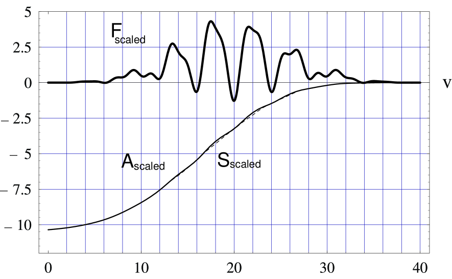
Figure 1: Flux, horizon area, and black hole entropy as functions of $v$ for $T_{0}=40$, $T_{1}=4$, $a_{0}=0.16=2a_{1}$, and $\xi=1/6$. The plotted rescaled quantities are: $F_{scaled}=3.2\times 10^{6}\,T_{vv},\,A_{scaled}=10^{4}\,(A-A_{f})/A_{f}$, and $S_{scaled}=10^{4}\,(S-S_{f})/S_{f}$, respectively. The behavior of the horizon area and the entropy are almost the same.

Case (ii): Choose $T_{0}=400$, $T_{1}=40$, and $\xi=1/6$. From Eq. (59), $a_{0}<6.96$. We again choose $a_{0}=0.16$ and $a_{1}=0.5a_{0}$. The behavior of the flux, the horizon area, and the entropy are shown in Fig. 2. The plotted rescaled quantities are: $F_{scaled}=1.6\times 10^{8}\,T_{vv},\,A_{scaled}=10^{5}\,(A-A_{f})/A_{f}$, and $S_{scaled}=10^{5}\,(S-S_{f})/S_{f}$. There are again three negative energy pulses. However, in this case, each pulse lasts sufficiently long enough that the acausal behavior of the horizon is not sufficient to rescue the GSL, as evidenced by the three periodic decreases of the horizon area. That is, if the entropy were simply given by $S=A/4$, as in the usual case, then the GSL would be violated during the periods of area decrease. What prevents this from occurring in this case is the influence of the scalar field term in the formula for the black hole entropy. Note also the phase lag between the change of sign of the flux and the onset of area decrease or increase. The scaling factors used in the two figures are different. The values of the scalar field on the horizon are approximately the same in both cases, and hence the magnitude of the fractional difference between $S$ and $A$ are of the same order of magnitude. However, the magnitude of the flux is smaller in Fig. 2 than in Fig. 1, because of the slower rate of change of $\phi$.

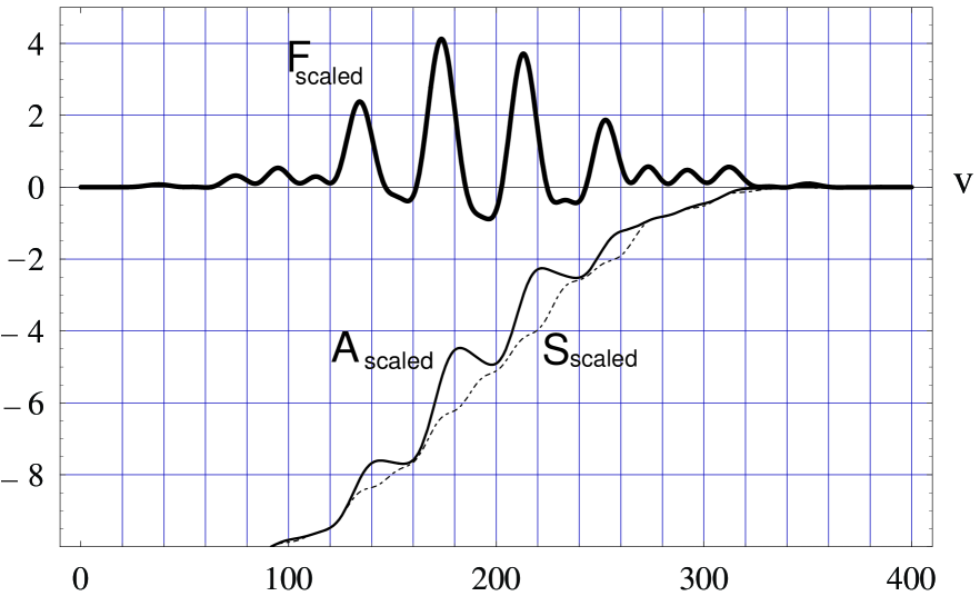
Figure 2: Flux, horizon area, and black hole entropy as functions of $v$ for $T_{0}=400$, $T_{1}=40$, $a_{0}=0.16=2a_{1}$, and $\xi=1/6$. The plotted rescaled quantities are: $F_{scaled}=1.6\times 10^{8}\,T_{vv},\,A_{scaled}=10^{5}\,(A-A_{f})/A_{f}$, and $S_{scaled}=10^{5}\,(S-S_{f})/S_{f}$, respectively. Here the horizon area undergoes periodic decreases, but the entropy is always non-decreasing.

5 Conclusions

We have demonstrated that classical massless non-minimally coupled scalar fields can be used to produce disturbingly large negative energy fluxes, even in flat spacetime. These classical negative energy fluxes are temporary in the sense that the time-integrated flux is always positive. However, unlike the situation in quantum theory, there are no constraints here analogous to the quantum inequalities. Therefore, it is possible for such fluxes to be sustained over macroscopically long time intervals. These fluxes appear to have magnitudes sufficient to produce gross violations of the second law of thermodynamics.

However, whether such violations occur could depend on the details of how these fields interact with matter. In an attempt to circumvent this issue, we examined these negative energy fluxes in the presence of a relatively unambiguous energy detector, a black hole. We considered scenarios in which a negative energy flux, composed of classical non-minimally coupled scalar fields, is injected into the black hole. It was proved that the GSL is in fact always satisfied. This conclusion is true for any positive or negative value of the coupling parameter, subject to the condition that $(1-8\pi\xi\,\phi^{2})>0$, and is independent of the scalar potential $V(\phi)$. The proof is also not restricted to Schwarzschild black holes, and therefore will hold for rotating black holes as well. The validity of the GSL hinges on two key effects - the acausal behavior of the event horizon and the presence of an additional term in the formula for the black hole entropy which depends on the scalar field.

In the dynamical case, the area of the event horizon, in contrast to that of the apparent horizon, depends upon the future history of the spacetime. This behavior is reviewed and illustrated in the Appendix. For a Schwarzschild black hole, when the temporal separation of the negative and positive energy pulses is no more than several times $M$, as was the case in Fig. 1, this effect alone can be sufficient to preserve the GSL. Here the horizon moves outward in anticipation of the (larger) positive energy in such a way that $A$ is non-decreasing.

If, however, the temporal separation becomes long compared to $M$, this effect is no longer sufficient to prevent $A$ from decreasing. This behavior is illustrated in Fig. 2. A similar result was found in the case of Brans-Dicke theory in Ref. [32]. Here the $\phi$-dependence of $S$ is crucial for insuring that the entropy is non-decreasing. Note that this $\phi$-dependence is also not always sufficient by itself to save the GSL without the acausal behavior of the horizon. For example, the product of the area of the apparent horizon times $(1-8\pi\xi\,\phi^{2})$ can decrease.

There are still some questions left unanswered at this point. One is whether negative energy could actually destroy a black hole. Our treatment in Sect. 3.2 and those in Refs. [26, 28] have assumed either a final black hole or cosmic censorship, and hence do not rule out this possibility. Another question is whether one could violate the GSL if $(1-8\pi\xi\,\phi^{2})$ is not positive everywhere; this situation would involve either super-Planckian values of the scalar field or very large values of the coupling parameter. It might also result in a sign change of the effective local Newton’s constant, given by Eq. (31), and non-positivity of the entropy density. Recall that this condition played a crucial role at several steps. We assumed it in our proof of the GSL, and it is also needed to define the transformations from the Jordan to the Einstein frame, and hence to make the argument that the area in the Einstein frame provides a suitable non-decreasing quantity. It may also be necessary for the initial value problem to be well-posed [33]. If $(1-8\pi\xi\,\phi^{2})\rightarrow 0$, then one would expect the effective stress tensor to become singular. This should lead to a backreaction effect which will prevent the system from actually reaching $(1-8\pi\xi\,\phi^{2})=0$; such an effect was indeed found in the case of cosmological spacetimes in Ref. [34]. However, $T_{\mu\nu}$ can remain finite if the numerator in Eq. (4) vanishes at the same points that $(1-8\pi\xi\,\phi^{2})\rightarrow 0$. This is what happens in some of the solutions of Barcelo and Visser [15, 16, 17]. Whether one could similarly construct examples which violate the GSL when $(1-8\pi\xi\,\phi^{2})\leq 0$ remains unknown, although we strongly suspect so. Nonetheless, it is quite interesting that, even for relatively weak fields and coupling constants: (a) one can get large sustainable, albeit temporary, classical negative energy fluxes, and (b) that such fluxes do not violate the GSL.

The acausal nature of the area of the event horizon is a disturbing feature of the current formulation of black hole thermodynamics, and one which has drawn the attention of various authors [35]. It is not clear whether this feature will survive in future theories. A definition of entropy based on a statistical mechanical enumeration of states would seem to have to be causal. This is a deep question which may have to await a more complete quantum theory of gravity for a resolution.

Finally, there is the question of whether the large negative energy associated with a classical scalar field could produce any dramatic effects, such as violations of the second law for an ordinary thermodynamic system. More generally, does this negative energy produce any observable effect on ordinary matter? It would seem rather peculiar if one could violate the ordinary second law but not the GSL. One would suspect that they should either both hold or both be violated. However at present we do not know of a similar general argument that would guarantee that the ordinary second law is not violated.

If such classical scalar fields can exist, that raises the question of why only certain classical fields are capable of producing large energy condition violations. For example, it is often thought that the conformally coupled scalar field is “physically reasonable” because it faithfully mimics certain aspects of the electromagnetic field. But why then does the classical electromagnetic field obey the WEC, while the conformally coupled scalar field does not?

It is usually easier to get negative energy in the context of quantum rather than classical fields. Moreover, in the regime of quantum fields, there seem to be some rather strong restrictions imposed on the magnitude and extent of negative energy densities and fluxes, in the form of the quantum inequalities. Given that nature seems to tightly restrict quantum violations of the weak energy condition, how seriously should one take classical violations? These are all issues for further enquiry.

Acknowledgments

The authors would like to thank Ted Jacobson for stimulating criticisms and correspondence, and Bob Wald, Bill Hiscock, and Matt Visser for key observations. We also thank Paul Anderson, Carlos Barcelo, Arvind Borde, Éanna Flanagan, Jaume Garriga, and Alex Vilenkin for useful comments and discussions. TAR would like to thank the members of the Tufts Institute of Cosmology for their hospitality while this work was being done. This research was supported by NSF Grant No. Phy-9800965 (to LHF) and by NSF Grant No. Phy-9988464 (to TAR).

6 Appendix

In this appendix we analyze the simple case of a spherical $\delta$-function pulse of positive energy imploding onto an already-existing black hole. We examine this case for two reasons. The first is to illustrate the somewhat counter-intuitive dynamical behavior of the horizon which is important in our discussion. The second is to present this calculation in a pedagogically detailed form - one which we have been unable to find in the standard literature.

For simplicity, we consider a Schwarzschild black hole of initial mass $M_{0}$, which absorbs a spherically symmetric $\delta$-function pulse of positive energy null fluid and becomes a black hole of mass $M$. Let $\lambda$ be the affine parameter on the horizon and suppose that the pulse intersects the horizon at $\lambda=0$. In the case of a spherically symmetric pulse the Raychaudhuri equation for the null generators of the horizon reduces to the simple form

$$\frac{d\theta}{d\lambda}=-\frac{{\theta}^{2}}{2}-R_{\mu\nu}k^{\mu}k^{\nu}\,.$$ (60)

For positive energy $R_{\mu\nu}k^{\mu}k^{\nu}=8\pi T_{\mu\nu}k^{\mu}k^{\nu}>0$, so set $R_{\mu\nu}k^{\mu}k^{\nu}=a\delta(\lambda)$, where $a$ is a positive constant.

Let us first solve the Raychaudhuri equation without the $\delta$-function term:

$$\frac{d\theta}{d\lambda}=-\frac{{\theta}^{2}}{2}\,.$$ (61)

This equation has the simple solution

$$\theta=\frac{2}{\lambda+{\lambda}_{0}}\,.$$ (62)

After the absorption of the pulse the generators of the horizon have zero expansion, so we want $\theta=0$ for $\lambda>0$, so let

$$\theta(\lambda)=\left\{\matrix{0\,,&\,\,\lambda>0\cr 2/(\lambda+{\lambda}_{0})\,,&\,\,\lambda<0}\right.\,,$$ (63)

i. e. , $\theta$ jumps discontinuously from $2/\lambda_{0}$ to $0$ as $\lambda$ passes through $0$. This gives us a $\delta$-function term in $d\theta/d\lambda$ of $-2\delta(\lambda)/{\lambda}_{0}$. Thus the above form of $\theta$ is a solution of

$$\frac{d\theta}{d\lambda}=-\frac{{\theta}^{2}}{2}-a\delta(\lambda)\,,$$ (64)

if $a=2/{\lambda}_{0}$, or ${\lambda}_{0}=2/a$. (The divergence of $\theta$ at $\lambda=-2/a$ represents a conjugate point in the distant past, which will be discussed later.)

Let us now generalize our solution slightly by assuming that the pulse intersects the horizon not at $\lambda=0$, but at $\lambda=\lambda_{+}$. Then our solution for $\theta$ becomes

$$\theta(\lambda)=\left\{\matrix{0\,,&\,\,\lambda>\lambda_{+}\cr 2/(\lambda-\lambda_{+}+2/a)\,,&\,\,\lambda<\lambda_{+}}\right.\,.$$ (65)

For the $\delta$-function pulse case, in the region where $\lambda<\lambda_{+}$, we can then integrate Eq. (45) to get

$${\rm ln}\,A=2\,{\rm ln}\,(\lambda-\lambda_{+}+2/a)+C\,.$$ (66)

We fix the constant of integration $C$ by the requirement that $A\rightarrow A_{f}=$ final horizon area as $\lambda\rightarrow\lambda_{+}$, so we have

$$C={\rm ln}\,A_{f}-2\,{\rm ln}\,(2/a)\,.$$ (67)

Our expression for $A$ then becomes

$$A(\lambda)=A_{f}\,{\left(\frac{\lambda-\lambda_{+}+2/a}{2/a}\right)}^{2}\,,\,\,\lambda<\lambda_{+}\,,$$ (68)

or

$$A(v)=A_{f}\,{\left[\frac{a(e^{\kappa v}-e^{\kappa v_{+}}+2\kappa)}{2\kappa}\right]}^{2}\,,\,\,v<v_{+}\,,$$ (69)

where we have used Eq. (48). We can write this in the form

$$A(v)=\left\{\matrix{A_{f}\,,&\,\,v\geq v_{+}\cr A_{f}\,{\left\{\left[a(e^{\kappa(v-v_{+})}-1)+2\kappa\,e^{-\kappa v_{+}}\right]/(2\kappa\,e^{-\kappa v_{+}})\right\}}^{2}\,,&\,\,v\leq v_{+}}\right.\,.$$ (70)

If $|v-v_{+}|\mathrel{\raise 1.29167pt\hbox{$>$\kern-7.5pt\lower 4.30554pt\hbox{$\sim$}}}{\kappa}^{-1}$, and since $v-v_{+}\leq 0$, then $e^{\kappa(v-v_{+})}\approx 0$, and we have

$$A \approx A_{f}\,{\biggl{[}{{2\kappa\,e^{-\kappa v_{+}}-a}\over{2\kappa\,e^{-\kappa v_{+}}}}\biggr{]}}^{2}$$ (71)

$$= A_{f}\,{\biggl{(}1-\frac{a}{2\kappa}\,e^{\kappa v_{+}}\biggr{)}}^{2}\equiv A_{0}\,.$$

Thus on a timescale of order ${\kappa}^{-1}=4M$, $A$ increases from $A_{0}$ to $A_{f}$. In the distant past (corresponding to $\lambda\rightarrow\lambda_{+}-2/a$), $A\rightarrow 0$, as can be seen from Eq. (68), but this is the conjugate point associated with the formation of the black hole or with the past singularity in the case of an eternal black hole. After the black hole forms, its area remains nearly constant until a few times $M$ before the positive pulse arrives at $v=v_{+}$.

We see that the horizon “anticipates” the subsequent arrival of the pulse. This counterintuitive acausal behavior arises from the way the horizon is defined. Recall that the horizon is defined as the boundary of past null infinity, i. e., the boundary of the region from which it is possible for light rays to escape to infinity (see, for example, Ref. [36], p. 300). Thus the horizon has the peculiar property that one must know the entire future evolution of the spacetime in order to know where the horizon intersects any given spacelike slice. For a static black hole, the null generators of the horizon have zero expansion. In order for the null generators in the horizon of the final (static) black hole to have zero expansion after the absorption of the pulse, the generators must have nonzero expansion prior to the pulse’s arrival. The null rays in the horizon of the final black hole are rays that would have escaped to infinity were it not for the arrival of the positive pulse, which refocused them to have zero expansion. (See Fig. 59 of Ref. [1], and the discussion in Ref. [37].)

Our calculation assumes that $\kappa$ is approximately constant and hence applies when the increase in area is small:

$$A_{f} = A_{0}\,{\biggl{(}1-\frac{a}{2\kappa}\,e^{\kappa v_{+}}\biggr{)}}^{-2}$$ (72)

$$\approx A_{0}\,{\biggl{(}1+\frac{a}{\kappa}\,e^{\kappa v_{+}}\biggr{)}}$$

$$= A_{0}+\Delta A\,.$$

If we take $A_{0}=16\pi{M_{0}}^{2}$ to be the initial area of the black hole in the distant past, where $M_{0}$ is its initial mass, then we have

$$\frac{\Delta A}{A_{0}}\approx\frac{a}{\kappa}\,e^{\kappa v_{+}}=2\,\,\frac{\Delta M}{M_{0}}\,.$$ (73)

In this approximation, the change in the mass of the black hole is

$$\Delta M = \frac{a}{2\kappa}\,M_{0}\,e^{\kappa v_{+}}$$ (74)

$$= \frac{a\,A_{0}}{8\pi}\,e^{\kappa v_{+}}\,,$$

where we have used $\kappa=1/(4M)\approx 1/(4M_{0})$. This agrees with the result obtained by calculating the change in mass directly from Eq. (22).

Let us now check that the conjugate point which appears in our solution occurs in the distant past. From Eq. (65) we see that the conjugate point occurs at

$$\lambda=\lambda_{c}=\lambda_{+}-\frac{2}{a}\,.$$ (75)

Using Eqs. (48) and (74), one can obtain

$$a=\frac{2\,\Delta M}{M_{0}\,\lambda_{+}}\,,$$ (76)

and so

$$\lambda_{c}=\lambda_{+}-\frac{M_{0}\,\lambda_{+}}{\Delta M}=\lambda_{+}\,\biggl{(}1-\frac{M_{0}}{\Delta M}\biggr{)}\,.$$ (77)

Since in our approximation $\Delta M\ll M_{0}$, $\lambda_{c}<0$ and $|\lambda_{c}|\gg\lambda_{+}$. Note that $\lambda=0$, or equivalently $v=-\infty$ or $V=0$, corresponds to the intersection of the past and future horizons in the maximally extended Schwarzschild spacetime. Thus for an eternal black hole, the conjugate point cannot occur to the future of the past horizon. In the case of a black hole formed from collapse, the same parameterization of $\lambda$ yields $\lambda>0$ everywhere on the future horizon outside of the collapsing body. In either case, $\lambda_{c}<0$ implies that the conjugate point occurs in the distant past.

References

- [1] S.W. Hawking and G.F.R. Ellis, The Large Scale Structure of Spacetime (Cambridge University Press, London, 1973), p. 88-96.
- [2] H. Epstein, V. Glaser, and A. Jaffe, Nuovo Cim. 36, 1016 (1965).
- [3] M. Morris and K. Thorne, Am. J. Phys. 56, 395 (1988).
- [4] M. Morris, K. Thorne, and U. Yurtsever, Phys. Rev. Lett. 61, 1446 (1988).
- [5] M. Alcubierre, Class. Quantum Grav. 11, L73 (1994).
- [6] L.H. Ford and T.A. Roman, Phys. Rev. D 53, 5496 (1996), gr-qc/9510071.
- [7] M.J. Pfenning and L.H. Ford, Class. Quantum Grav. 14, 1743 (1997),gr-qc/9702026.
- [8] N.A. Chernikov and E.A. Tagirov, Ann. Inst. Henri Poincaré 9, 109 (1968).
- [9] C.G. Callen, Jr., S. Coleman, and R. Jackiw, Ann. Phys. (NY) 59, 42 (1970).
- [10] L. Parker, Phys. Rev. D 7, 976 (1973).
- [11] J.D. Bekenstein, Ann. Phys. (NY) 82, 535 (1974).
- [12] J.D. Bekenstein, Phys. Rev. D 11, 2072 (1975).
- [13] S. Deser, Phys. Lett. B134, 419 (1984).
- [14] É.É. Flanagan and R.M. Wald, Phys. Rev. D 54, 6233 (1996).
- [15] C. Barcelo and M. Visser, Phys. Lett. B466, 127 (1999), gr-qc/9908029.
- [16] C. Barcelo and M. Visser, Energy Conditions and Their Cosmological Implications, gr-qc/0001099.
- [17] C. Barcelo and M. Visser, Class. Quantum Grav. 17 3843 (2000), gr-qc/0003025.
- [18] L.H. Ford, Proc. Roy. Soc. Lond. A 364, 227 (1978).
- [19] L.H. Ford, Phys. Rev. D 43, 3972 (1991).
- [20] J.D. Bekenstein, Phys. Rev. D 9, 3292 (1974).
- [21] L.H. Ford and T.A. Roman, Phys. Rev. D 46, 1328 (1992).
- [22] V. Iyer and R.M. Wald, Phys. Rev. D 50, 846 (1994); Phys. Rev. D 52, 4430 (1995).
- [23] M. Visser, Phys. Rev. D 48, 5697 (1993).
- [24] M. Visser, Phys. Rev. D 48, 583 (1993).
- [25] V. Faraoni, E. Gunzig, and P. Nardone, Fund. Cosmic Phys. 20, 121 (1999), gr-qc/9811047.
- [26] T. Jacobson, G. Kang, and R.C. Myers, Phys. Rev. D 52, 3518 (1995), gr-qc/9503020; Black Hole Entropy in Higher Curvature Gravity, gr-qc/9502009; Phys. Rev. D 49, 6587 (1994), gr-qc/9312023.
- [27] We thank Ted Jacobson for this argument.
- [28] G. Kang, Phys. Rev. D 54, 7483 (1996); gr-qc/9606020.
- [29] R. M. Wald, Quantum Field Theory in Curved Spacetime and Black Hole Thermodynamics, (The University of Chicago Press, Chicago, 1994).
- [30] See Eq. (134) of M.J. Pfenning and L.H. Ford, Phys. Rev. D 57, 3489 (1998), gr-qc/9710055, which is based on the work of B.P. Jensen, J.G. McLaughlin, and A.C. Ottewill, Phys. Rev. D 45, 3002 (1992).
- [31] We are grateful to Bob Wald for first pointing this out to us.
- [32] M.A. Scheel, S.L. Shapiro, and S.A. Teukolsky, Phys. Rev. D 51, 4236 (1995).
- [33] É.É. Flanagan, talk given at the “KipFest” meeting, Cal Tech, June 2000.
- [34] A. Saa, E. Gunzig, L. Brenig, V. Faraoni, T.M. Rocha Filho, and A. Figueiredo, Superinflation, quintessence, and the avoidance of the initial singularity, gr-qc/0012105.
- [35] For a good recent review, see A. Corichi and D. Sudarsky, When is ?, gr-qc/0010086.
- [36] R. M. Wald, General Relativity, (The University of Chicago Press, Chicago, 1984).
- [37] V.P. Frolov and I.D. Novikov, Black Hole Physics: Basic Concepts and New Developments, (Kluwer Academic Publishers, Dordrecht, 1998), p. 173-175.