[

Computing the Complete Gravitational Wavetrain from Relativistic Binary Inspiral

Abstract

We present a new method for generating the nonlinear gravitational wavetrain from the late inspiral (pre-coalescence) phase of a binary neutron star system by means of a numerical evolution calculation in full general relativity. In a prototype calculation, we produce 214 wave cycles from corotating polytropes, representing the final part of the inspiral phase prior to reaching the ISCO. Our method is based on the inequality that the orbital decay timescale due to gravitational radiation is much longer than an orbital period and the approximation that gravitational radiation has little effect on the structure of the stars. We employ quasi-equilibrium sequences of binaries in circular orbit for the matter source in our field evolution code. We compute the gravity-wave energy flux, and, from this, the inspiral rate, at a discrete set of binary separations. From these data, we construct the gravitational waveform as a continuous wavetrain. Finally, we discuss the limitations of our current calculation, planned improvements, and potential applications of our method to other inspiral scenarios.

]

The inspiral and coalescence of binary neutron stars are among the most promising sources of gravitational radiation for the laser interferometer gravitational wave observatories LIGO, VIRGO, GEO, and TAMA, which should become operational in a few years. It is estimated [1] that LIGO/VIRGO will be able to detect the last 15 minutes of the inspiral (16,000 orbits) of a typical binary neutron star system. Detection and analysis of the signal will depend on matched filter techniques, which require theoretical templates of the waveforms.

The evolution of binary neutron stars proceeds in different stages. By far the longest is the initial quasi-equilibrium inspiral phase, during which the stars move in nearly circular orbits, while the separation between the stars slowly decreases as energy is carried away by gravitational radiation. The quasi-circular orbits become unstable at the innermost stable circular orbit (ISCO), where the inspiral enters a plunge and merger phase. The merger and coalescence of the stars happens on a dynamical timescale, and produces either a black hole or a larger neutron star, which may collapse to a black hole at a later time. The final stage of the evolution is the ringdown phase, during which the merged object settles down to equilibrium.

Two distinct approaches have commonly been employed in general relativity to study the inspiral phase. Much progress has been made in post-Newtonian (PN) studies of compact binaries (see, e.g. [2], and references therein). Most of these approaches, however, approximate the stars as point sources, which neglects important finite-size effects for neutron stars. Also, PN expansions may not converge sufficiently rapidly in the strong-field region near the ISCO. In an independent approach, relativistic quasi-equilibrium models of the inspiral phase of neutron star binaries have been constructed numerically (see, e.g., [3] for corotating binaries and [4] for the more realistic case of irrotational binaries). Binaries have also been evolved using fully relativistic hydrodynamics [5, 6], but computational constraints limit these evolutions to a few orbits.

In this paper, we propose a “hydro without hydro” method for using the “snapshots” generated by quasi-equilibrium codes to create a complete wavetrain [7, 8]. We use these snapshots to find the gravitational waveform at a given separation and construct an effective radiation reaction. From this, the inspiral rate is known, and the entire wavetrain can be constructed. We describe this method below. We then present the results of a prototype calculation, and discuss its implications.

The fundamental assumption in the quasi-equilibrium approximation is that the orbital timescale is much shorter than the gravitational radiation reaction timescale. The binary inspiral then proceeds along a sequence of quasi-equilibrium configurations in nearly circular orbits with constant rest mass $M_{0}$. This assumption significantly simplifies the problem, since the hydrodynamical equations can be integrated to yield a relativistic Bernoulli equation [3]. A similar approximation is routinely adopted in stellar evolution calculations. There too, the evolutionary timescale is much longer than the hydrodynamical timescale, so that the star can safely be assumed to be in quasi-equilibrium on a dynamical timescale.

Constructing quasi-equilibrium binary configurations yields their total mass-energy $M(r)$ and their orbital angular frequency $\Omega_{\rm orb}(r)$ as a function of separation $r$. The ISCO of an evolutionary $M_{0}=const$  sequence, where the assumption of quasi-equilibrium breaks down, can be identified by locating a turning point along an $M$ versus $r$ curve (see, e.g., the cross in Fig. 1).

Given a relativistic quasi-equilibrium configuration, we can compute the emitted gravitational radiation by employing the binary data for the matter source terms in Einstein’s field equations. In particular, the gravitational fields can be evolved in the presence of these predetermined matter sources with a relativistic evolution code (“hydro without hydro”, [8]). There is no need to re-solve any of the hydrodynamic equations for the source, as we are assuming that the stars move in circular orbits and are little affected by the waves. We thus simply rotate the source terms on our numerical grid. Repeating this calculation for members of an evolutionary sequence at discrete separations $r$, we obtain the wave amplitude $A(r)$ and the orbit-averaged gravitational wave luminosity $<dM/dt>(r)$ at these separations. A fitting function can then be used to interpolate to any intermediate separation (see Fig. 1).

The inspiral is determined by computing the effective radiation reaction due to the radiation of mass-energy by gravitational waves. The energy loss $<dM/dt>$ forces the binary to a closer separation, as it “slides down” the quasi-equilibrium $M$ vs $r$ curve. The inspiral rate is thus

$${dr\over dt}={<dM/dt>\over(dM/dr)_{\rm eq}},$$ (1)

Solving this equation determines $r$ as a function of time $t$, which then allows us to express $A(t)$ and $\Omega_{\rm orb}(t)$ in terms of $t$. The complete quasi-equilibrium wavetrain can then be constructed from

$$r_{s}h(t)=A(t)\sin\bigl{(}\int_{0}^{t}\Omega_{\rm GW}(t^{\prime})dt^{\prime}\bigr{)}\,,$$ (2)

where we expect $\Omega_{\rm GW}\approx 2\Omega_{\rm orb}$ due to the $m=2$ dominance of the radiation, and where $r_{s}$ is the distance between the source and the distant observer. The validity of our method and its ability to produce reliable wavetrains is most easily demonstrated in relativistic scalar gravitation, where the quasi-equilibrium wavetrain can be compared to an exact numerical solution [9].

In the following we present a prototype calculation which employs the quasi-equilibrium models of Baumgarte et.al. [3]. These models assume maximal slicing $K\equiv K^{i}_{~{}i}=0$, where $K_{ij}$ is the extrinsic curvature, and spatial conformal flatness, so that the spatial metric $\gamma_{ij}$ can be written as a product of the conformal factor $\psi$ and a flat metric $f_{ij}$, $\gamma_{ij}=\psi^{4}f_{ij}$. The latter is believed to approximately minimize the gravitational wave content of the spacetimes [10] while introducing only small deviations from correct evolutionary sequences [11]. The stars are modeled as corotating polytropes $P=\kappa\rho_{0}^{1+1/n}$ with polytropic index $n=1$. We non-dimensionalize our results by setting $\kappa=1$. In addition to the matter profile, these models provide the conformal factor $\psi$, the lapse function $\alpha$ and the shift vector $\beta^{i}$.

We insert these quasi-equilibrium data into our relativistic evolution code, which is based on a conformal decomposition of the ADM equation [12]. This decomposition conveniently splits the fundamental variables into longitudinal quantities ($\psi$ and $K$) and “wave-like” transverse quantities (the conformally related metric $\tilde{\gamma}_{ij}$ and the tracefree part of the extrinsic curvature $\tilde{A}_{ij}$). We also introduce “conformal connection functions” $\tilde{\Gamma}^{i}$ as independent auxiliary quantities, which improves numerical stability dramatically (cf. [13]).

We insert “by hand” the matter variables, the gauge variables ($\alpha$ and $\beta^{i}$) and the longitudinal quantities ($\psi$ and $K=0$) for all times, appropriately rotated by $d\phi/dt=\Omega_{\rm orb}$ [14]. The transverse variables ($\tilde{\gamma}_{ij}$, $\tilde{A}_{ij}$ and $\tilde{\Gamma}^{i}$) are evolved dynamically, adopting the quasi-equilibrium data $\tilde{A}_{ij}$, $\tilde{\gamma}_{ij}=f_{ij}$ and $\tilde{\Gamma}^{i}=0$ as initial data. We found that we could reduce the numerical errors by explicitly splitting quasi-equilibrium “background” terms from dynamically evolved terms in the evolution equation for the $\tilde{\Gamma}^{i}$.

FIG. 1.: Total mass $M$ and gravitational wave luminosity $dM/dt$ versus separation for our evolutionary sequence. Both quantities are measured by a distant observer. The separation is parameterized by $z_{A}$ (see text). The points represent individual numerical models, and the solid lines are fits. The turning point $dM/dz_{A}=0$ in the top panel locates the ISCO (marked by the cross).

We evolve on a 120$\times$120$\times$60 zone grid, imposing equatorial symmetry across the z-axis. Each star is covered by roughly 8 points across a diameter. We impose approximate outgoing wave boundary conditions on the transverse variables at a separation of $0.1\lambda_{\rm GW}$ - $0.3\lambda_{\rm GW}$, where $\lambda_{\rm GW}$ is a gravitational wavelength. We expect our outer boundary location to be one of the primary sources of error (see discussion below, and compare with [6] where the boundaries are similarly placed). We monitor the violation in the Hamiltonian and momentum constraints and find that they are all satisfied quite well and that the degrees of violation do not grow significantly with time. We doubled the resolution for one configuration, and found that $A$ changed by only $\approx$ 2%.

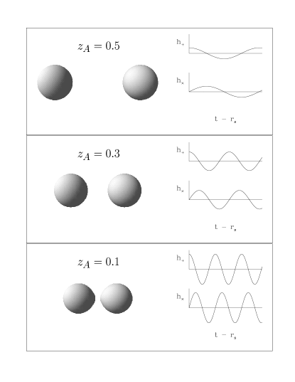
FIG. 2.: Three representative binary configurations with their corresponding waveforms. We show the binaries with greatest and smallest separation in our sequence, and one intermediate member. At right, the two polarizations of gravity waves ($h_{+}$ and $h_{\times}$) along the $z$-axis are shown. On the $z$-axis, the two polarizations only differ by a phase.

To extract gravitational waves, we match to even-parity Moncrief variables $\psi_{lm}$ (or Zerilli functions) at the outer part of the grid (see [15, 16, 17] for details). For simplicity, we focus on $l=2$, $m=\pm 2$ modes, which we expect to be dominant. We have checked that the contribution to the energy flux of the $l=4$, $m=\pm 4$ mode is very small ($\sim 4$%), and that of the $l=2$, $m=0$ mode negligible ($<10^{-6}$). Assuming $l=2$, $m=\pm 2$ dominance, we have

$$\displaystyle\frac{dM}{dt} = \displaystyle\frac{1}{32\pi}\left((\partial_{t}\psi_{22})^{2}+(\partial_{t}\psi_{2-2})^{2}\right)$$ (3)

$$A = \displaystyle\sqrt{{5\over 16\pi}\left(\overline{\psi}^{2}_{22}+\overline{\psi}^{2}_{2-2}\right)}$$ (4)

where $\overline{\psi}_{2\pm 2}$ denotes the amplitude of $\psi_{2\pm 2}$. We approximate the asymptotic value of $\overline{\psi}_{lm}$ by its value at the edge of our numerical grid. Due to our neglect of self-consistent transverse fields in the initial data, we find a transient noise in the waveforms during the first light-crossing time. After that time we observe the expected periodic waveforms originating from the periodic binary orbit.

FIG. 3.: The amplitude $A$ and angular frequency $\Omega_{\rm GW}$ of the gravitational wave signal as a function of retarded time $t-r_{s}$ (solid line). The dotted line is the result for Newtonian point masses in the quadrupole approximation. The top label provides times in seconds for a binary of total rest mass $M_{0}=2\times 1.5M_{\odot}$. Our sequence ends at a frequency $\Omega_{\rm GW}=2.36$ kHz for such a binary.

We constuct 14 different configurations along a sequence of constant total rest mass $M_{0}=2\times 0.1$ in our nondimensional units. The rest mass of the individual stars is about 55% of the maximum allowed rest mass of an isolated, nonrotating star. We parameterize the binary separation by the dimensionless quantity $z_{A}$, the ratio of the separation between the innermost points and the outermost points on the stars (see [3]). In terms of $z_{A}$, touching binaries correspond to $z_{A}=0$ and infinitely separated configurations to $z_{A}=1$. In the top panel of Fig. 1, we plot the ADM mass $M$ as a function of separation, and in the bottom panel the gravitational wave luminosity $dM/dt$ as inferred from our “hydro without hydro” integrations. Since we expect our quasi-equilibrium method to break down at the ISCO, we construct waveforms for configurations with $z_{A}\geq 0.1$, which is close to but safely outside the ISCO. In Fig. 2 we illustrate three of these configurations together with their extracted waveforms. In Fig. 3 we show the wave amplitude $A$ and the gravitational wave frequency $\Omega_{\rm GW}$ as a function of retarded time. The solid line is our numerical result, which we compare with the wavetrain of a Newtonian point mass system as computed from the quadrupole approximation (dotted line). The difference is caused by differences in the binding energy and the gravitational wave luminosity due to relativity, as well as the numerical limitations of our calculation (see discussion below). Finally, we construct the continuous gravitational wavetrain from $A$ and $\Omega_{\rm GW}$, shown in Fig. 4.

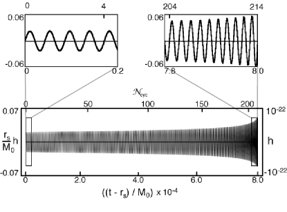
FIG. 4.: The full wavetrain $h_{+}$ or $h_{\times}$ on the $z$-axis as a function of retarded time and cycle number. The top two panels show enlargements of the first four and last ten cycles. We also indicate the gravitational strain $h$ for a binary of total rest mass $M_{0}=2\times 1.5M_{\odot}$ at a separation of 100 Mpc.

In summary, we propose a new technique to construct gravitational wavetrains from inspiraling relativistic binaries and demonstrate the feasability of this technique by a numerical example. Our scheme is extremely efficient computationally. For the computational cost of 14 orbits, we produced the complete wavetrain covered by our sequence (214 cycles). There is no reason why one could not, with more points along the sequence, produce many more cycles of the inspiral.

It is clear, however, that several improvements must be implemented to produce more accurate and reliable wavetrains. Our outer boundary conditions are crude and imposed at too small a separation. To gauge the error of our simplistic wave extraction, we measured $\overline{\psi}_{22}$ at 0.23$\lambda_{\rm GW}$ and at 0.35$\lambda_{\rm GW}$ and found a difference of roughly 10%. Gravitational waves should be extracted in the wave zone $r_{s}>\lambda_{\rm GW}$, or more sophisticated boundary conditions and wave extraction should be applied (e.g. [18]). Furthermore, the assumption of corotation is not realistic; using irrotational sequences is more physical [19]. Finally, one could consider iterating this method by adding the radial velocity to the source and incorporating the calculated transverse components of the field, as well as deviations from conformal flatness, and then recomputing the waves and inspiral.

The binary black hole inspiral problem could be approached in a similar way [20]. This is a prospect we are currently investigating.

It is a pleasure to thank Masaru Shibata for stimulating discussions and useful suggestions. We would also like to thank REU students H. Agarwal, E. Engelhard, K. Huffenberger, P. McGrath, J. Mehl, and D. Webber for assistance on Figures 2 and 4. TWB gratefully acknowledges support through a Fortner Fellowship. Much of the calculation and visualization were performed at the National Center for Supercomputing Applications at UIUC. This paper was supported in part by NSF Grants AST 96-18524 and PHY 99-02833 and NASA Grant NAG 5-7152 to UIUC.

REFERENCES

- [1] K. S. Thorne, in Black Holes and Relativistic Stars, edited by R.M. Wald (U. of Chicago Press, Chicago, 1998), p. 59.
- [2] L. Blanchet, T. Damour, B.R. Iyer, C.M. Will, and A.G. Wiseman, Phys. Rev. Lett 74 3515 (1995).
- [3] T. W. Baumgarte, G. B. Cook, M. A. Scheel, S. L. Shapiro and S. A. Teukolsky, Phys. Rev. Lett. 79, 1182 (1997); Phys. Rev. D 57, 7299 (1998).
- [4] S. Bonazzola, E. Gourgoulhon, and J.A. Marck, Phys. Rev. Lett. 82, 892 (1999); P. Marronetti, G. J. Mathews and J. R. Wilson, Phys. Rev. D 60, 087301 (1999); K. Uryu and Y. Eriguchi, Phys. Rev. D 61, 124023 (2000).
- [5] M. Shibata, Phys. Rev. D 60, 104052 (1999)
- [6] M. Shibata and K. Uryu, Phys. Rev. D 61, 064001 (2000).
- [7] S. Shapiro, paper presented at Binary Neutron Star Grand Challenge Workshop, NCSA, January 1997.
- [8] T. W. Baumgarte, S. A. Hughes, and S. L. Shapiro, Phys. Rev. D 60, 087501 (1999).
- [9] H.-J. Yo, T. W. Baumgarte and S. L. Shapiro, in preparation.
- [10] J. W. York, Jr., Phys. Rev. Lett. 26, 1656 (1971).
- [11] F. Usui, K. Uryu and Y. Eriguchi, Phys. Rev. D 61, 024039 (2000).
- [12] T. W. Baumgarte and S. L. Shapiro, Phys. Rev. D 59, 024007 (1999).
- [13] T. Nakamura, K. Oohara and Y. Kojima, Prog. Theor. Phys. Suppl. 90, 76 (1987).
- [14] We have verfied that dynamically evolving , and solving maximal slicing to find at each timestep yields very similar results.
- [15] V. Moncrief, Ann. Phys. 88, 323 (1974).
- [16] A. Abrahams et al., Phys. Rev. D 45, 3544 (1992).
- [17] M. Shibata and T. Nakamura, Phys. Rev. D 52, 5428 (1995).
- [18] N. T. Bishop, R. Gomez, P. R. Holvorcem, R. A. Matzner, P. Papadopoulos and J. Winicour, J. Comp. Phys. 136, 140 (1997); A. M. Abrahams et.al. (The Binary Black Hole Grand Challenge Alliance) Phys. Rev. Lett. 80, 1812 (1998).
- [19] C. S. Kockanck, Astrophys. J. 398 234 (1992); L. Bildsten and C. Cutler, Astrophys. J. 400, 175 (1992).
- [20] For black holes, the conserved quantity along a quasi-equilibrium sequence is the horizon area, conjectured to be an adiabatic invariant. See J.D. Bekenstein, in Black Holes, Gravitational Radiation and the Universe, edited by B.R. Iyer and B. Bhawal (Kluwer, Dordrecht, 1999), pp. 87-101.