Gravitational waves from a spinning particle scattered by a relativistic star:
Axial mode case

Abstract

We study gravitational waves from a spinning test particle scattered by a relativistic star using a perturbation method. The present analysis is restricted to axial modes. By calculating the energy spectrum, the waveforms and the total energy and angular momentum of gravitational waves, we analyze the dependence of the emitted gravitational waves on a particle spin. For a normal neutron star, the energy spectrum has one broad peak whose characteristic frequency corresponds to the angular velocity at the turning point (a periastron). Since the turning point is determined by the orbital parameter, there exists the dependence of the gravitational wave on a particle spin. We find that the total energy of $l=2$ gravitational waves gets larger as the spin increases in the anti-parallel direction to the orbital angular momentum. For an ultracompact star, in addition to such an orbital contribution, we find the quasi-normal modes exited by a scattered particle, whose excitation rate to gravitational waves depends on the particle spin. We also discuss the ratio of the total angular momentum to the total energy of gravitational waves and explain its spin dependence.

I Introduction

A neutron star binary is one of the most promising source for gravitational waves, which will be observed in the near future by gravitational wave interferometers such as Laser Interferometric Gravitational Wave Observatory (LIGO), VIRGO, GEO600, TAMA300, and Laser Interferometer Space Antenna (LISA) [1]. Since gravitational waves has a little interaction to the matter, we could resolve the phenomena of a strong gravitational field such as a black hole formation by the direct observation of gravitational waves, which can not be revealed completely only by electromagnetic waves. From such an analysis, we could find new information about the interior of a neutron star whose equation of state is not yet well-known. These expectations motivate theoretical efforts to investigate gravitational waves from a neutron star binary in the inspiral and merging phase.

One of the final step to calculate gravitational waves from a neutron star binary is a fully general relativistic simulation with no approximation. In the past decade, many efforts have been put into the 3D numerical simulation of merging a neutron star binary in Newtonian, post-Newtonian, and general relativity. However, Einstein equations are non-linear wave equations with constraints. The present simulation has still faced to many difficulties, however we hope that we will succeed to simulate some of limited cases in the near future. In such a situation, we may invoke another way to study gravitational waves from such a binary system by using some approximation methods focusing to some particular physical quantities and extract fundamental and important properties.

One of these approximate approaches of gravitational waves from a binary system is a perturbation method, in which a companion of the binary is treated as a test particle with mass $\mu$ moving around a relativistic background object with mass $M$ ($\gg\mu$). It has been shown that this approach gives a good approximation for gravitational waves from a head-on collision of two black holes [2], and it has been thought to be one of the reliable approximation for treating gravitational waves from a coalescing black hole binary.

This method can also apply to a neutron star binary, although so far there has been a strong restriction such that we assume a spherical symmetric background spacetime, which can be extended to a slow rotating background. The motion of a test particle excites nonradial pulsations of a central spherically symmetric star in the emission of gravitational waves. The perturbation equations of gravitational waves outside the spherical star are given by Regge and Wheeler [3] and Zerilli [4]. Regge-Wheeler-Zerilli equations are well-known as perturbation equations in the Schwarzschild background spacetime. While inside the star, the perturbation equations both for the metric and stellar fluid were derived by Thorne and Campolattaro [5], Lindblom and Detweiler [6], and Chandrasekhar and Ferrari [7].

For a spherically symmetric star, the perturbation equations are completely separated by its parity, i.e., polar (even) and axial (odd) modes. The polar mode contains two types of waves; gravitational waves and material waves which interact each other. While, the axial mode has only one type, i.e., gravitational waves. From this character, quasi-normal modes of fluid oscillations ($f$, $p$ and $g$ modes) are exited by a test particle only in polar modes, while the quasi-normal modes of gravitational waves ($w$ modes) will appear in both modes. As for the axial mode, since there is no fluid oscillation, only $w$ modes are excited.

In the case of a binary black hole system, it is known that gravitational waves are dominated by the quasi-normal modes at the ringing-down phase. Since the quasi-normal mode contains many information about the newly formed black hole or neutron star, the analysis of the quasi-normal modes is important in the relativistic astrophysics. As for a binary neutron star system, the remnant of merged binary stars with $M\sim 1.4M_{\odot}$ may form a black hole after a short time. The ringing-down phase of a neutron star binary may be determined by the quasi-normal modes of a black hole. However, since the quasi-normal modes of a star would also be excited at the inspiral phase, it is still important to focus on them.

For polar modes, Kojima [8] examined gravitational waves from a particle in a circular orbit around a spherically symmetric relativistic star. From the symmetry of a circular orbit, axial modes are completely canceled out in this case. He found the resonant oscillation of a star and an enhancement of gravitational waves at the same frequency of the quasi-normal mode.

For axial modes, Borrelli [9] calculated the energy spectrum when a particle is spiraling onto an ultracompact star ($R\lesssim 3M$). In the case of the ultracompact star, it is known that some quasi-normal modes are trapped by a potential barrier of gravitational waves. These quasi-normal modes are excited by a falling particle.

Several works for a scattered particle have been done. The present authors[10] calculated the energy spectrum for axial modes. In the case of neutron stars ($R\gtrsim 3M$), a single peak appears in the energy spectrum, which depends on the trajectory of a particle. On the other hand, in the case of ultracompact stars ($R\lesssim 3M$), many sharp peaks are also excited in the energy spectrum. Some peaks are explained by the quasi-normal modes trapped by the quasi-bound state in the potential, and the rest of peaks is due to the resonance of two propagating waves, which are reflected by the potential barrier or the infinite wall at the center of the star. These peaks never appear for the black hole case, because there are no bound state in the potential, and gravitational waves are purely incoming at the horizon, so the resonance of two reflected waves never occurs. Andrade and Price [11] also studied axial modes of gravitational waves by a scattered particle. They have found that even for stellar models with $R\gtrsim 3M$, a scattered particle with a very large orbital angular momentum could weakly excite quasi-normal modes. Ferrari, Gualtieri, and Borrelli [12] computed energy spectra of both polar and axial modes from a particle scattered by a polytropic star. In their results, fluid modes ($f$ and $p$ modes) are also excited in the energy spectrum.

Recently, there are two papers demonstrated gravitational waves from a scattered particle in a spherical symmetric star for time evolution. Ruoff, Laguna, and Pullin [13] computed spectrum and waveform for polar modes, focusing on the excitation of $w$-modes. They concluded that the excitation appeared in the spectrum, although $w$-modes significantly contributes to the energy in the case of the orbital speed $v>0.9c$. Ferrari and Kokkotas [14] also computed spectrum and waveform for axial modes. They also point out that most of the $w$-modes are indeed, clearly excited in the spectrum whose feature is the same to our previous results [10].

Neutron stars are usually rotating. Then it is very natural to take into account a rotation effect as a next step. From the viewpoint of the gravitational wave astronomy, a rotating relativistic star is a very important object, because there exists $r$ mode which shows very strong instability for any rotations [15] and this effect itself becomes one of the promising source of gravitational waves [16]. For example, hot young neutron stars would be enough rapidly rotating to occur $r$ mode instability, and would spin down toward a usual observed neutron star by radiating gravitational waves. The recent observation suggests that low mass X-ray binaries [17] would include a rapidly rotating neutron star.

Although there are several perturbation analysis for a slowly rotating neutron star, we have no systematic method to solve for the case of a rapidly rotating star except for the analysis of the neutral point [18]. Here, we propose an extremely simple model to treat some effect of a rapid rotation by adding a spin to a test particle. Since we can not take into account the structure of a test particle, we do not expect the excitation of a test particle itself, and then will not be able to discuss the wave mode of a spinning particle itself. However, this work might be a milestone for a further study of a rotation effect on gravitational waves from a binary system.

The spinning particle in a curved spacetime was formulated by Papapetrou [19] and Dixon [20] by taking a point particle limit of a relativistic extended body. In the case of a rotating black hole with a spinning test particle, which mimics a collision of two rotating black holes, there are several works using a perturbation approach. [21, 22, 23].

In this paper, we will examine gravitational waves from a spinning particle scattered by a relativistic star. We calculate the energy spectrum, the waveform and the total energy and angular momentum of the emitted gravitational waves, and investigate the spin effect to gravitational waves. This paper is organized as follows. In Sec. II, we briefly review the equation of motion of a spinning particle and gravitational waves in a spherically symmetric background using a perturbation theory. We show our numerical results in Sec. III. Section IV is devoted to discussion.

Throughout this paper, we adopt the units of $G=c=1$, where $G$ and $c$ denote the gravitational constant and speed of light respectively, and the metric signature of $(-,+,+,+)$.

II Perturbation equations for axial modes

A Spinning Particle

We briefly summarize the equations of motion of a spinning test particle and its energy-momentum tensor $T^{\mu\nu}$. The motion of a spinning test particle in a curved background is discussed by Papapetrou [19] and Dixon [20]. They presented the equation of motions for a spinning particle as

$$\frac{D}{d\tau}p^{\mu}(\tau) = -\frac{1}{2}R^{\mu}{}_{\nu\rho\sigma}(z(\tau))v^{\nu}(\tau)S^{\rho\sigma}(\tau),$$ (1)

$$\frac{D}{d\tau}S^{\mu\nu}(\tau) = p^{\mu}(\tau)v^{\nu}(\tau)-p^{\nu}(\tau)v^{\mu}(\tau),$$ (2)

where $z^{\mu}(\tau)$, $v^{\mu}(\tau)=dz^{\mu}/d\tau$, $p^{\mu}(\tau)$ and $S^{\mu\nu}(\tau)$ denote the trajectory of a particle, 4-velocity, 4-momentum, and spin tensor, respectively. The mass $\mu$ and the magnitude of a spin $S$, which are defined by $p_{\mu}p^{\mu}=-\mu^{2}$ and $S_{\mu\nu}S^{\mu\nu}=2S^{2}$, are conserved [24]. Since we also have to specify the center of mass, which supplies an additional condition, we assume

$$S^{\mu\nu}p_{\nu}=0,$$ (3)

with which we find a complete set of equations of motion. The normalization of the affine parameter $\tau$ is conveniently chosen as $u_{\mu}v^{\mu}=-1$, where $u^{\mu}(\equiv p^{\mu}/\mu)$ is the normalized momentum.

Since the total angular momentum of the particle is conserved, we can specify the $z$ axis (and then the equatorial plane) in Schwarzschild spacetime by the direction of the conserved total angular momentum $\vec{J}$, i.e., $\vec{J}=(0,0,J)$ with $J>0$. In this paper, we restrict a particle motion onto the equatorial plane $(\theta=\pi/2)$ in Schwarzschild background. By use of the conserved quantities [20] along the trajectory $z^{\mu}(\tau)$, we write down the equation of motion of the particle with the energy $\tilde{E}(\equiv E/\mu)$, total angular momentum $\tilde{J}(\equiv J/\mu)$ and spin $\tilde{S}(\equiv S/\mu)$ [25] as follows [23]:

$$\Sigma_{S}\Lambda_{S}\frac{dt}{d\tau} = \left(1-{2M\over r}\right)^{-1}\left(r^{2}\tilde{E}-\frac{M\tilde{S}}{r}\tilde{J}\right),$$ (4)

$$\Sigma_{S}^{2}\Lambda_{S}^{2}\left(\frac{dr}{d\tau}\right)^{2} = R_{S},$$ (5)

$$\Sigma_{S}\Lambda_{S}\frac{d\phi}{d\tau} = \left(1+\frac{3M\tilde{S}^{2}}{r\Sigma_{S}}\right)\left(\tilde{J}-\tilde{S}\tilde{E}\right),$$ (6)

where $\Sigma_{S}$, $\Lambda_{S}$ and $R_{S}$ are

$$\Sigma_{S} = r^{2}\left(1-\frac{M\tilde{S}^{2}}{r^{3}}\right),$$ (7)

$$\Lambda_{S} = 1-\frac{3M\tilde{S}^{2}r\left(\tilde{J}-\tilde{S}\tilde{E}\right)^{2}}{\Sigma_{S}^{3}},$$ (8)

$$R_{S} = \left(r^{2}\tilde{E}-\frac{M\tilde{S}}{r}\tilde{J}\right)^{2}$$ (10)

$$-r^{2}\left(1-{2M\over r}\right)\left[\frac{\Sigma_{S}^{2}}{r^{2}}+\left(\tilde{J}-\tilde{S}\tilde{E}\right)^{2}\right].$$

In what follows, we introduce the “orbital” angular momentum by $\tilde{L}=\tilde{J}-\tilde{S}$ which is same to Ref. [23], because the orbital angular momentum plays an important role in the gravitational wave in the case of a non-spinning particle [10]. Since we set $J>0$, the spin direction is classified by the sign of $S$ into the parallel ($S\geq 0$) and anti-parallel ($S\leq 0$) to the orbital angular momentum.

From Eq. (5), we can introduce the effective potential $\tilde{V}^{\rm(particle)}$ of a spinning particle in the equatorial plane, which is

$$\tilde{V}^{\rm(particle)}=\frac{-\beta+\sqrt{\beta^{2}-\alpha\gamma}}{\alpha},$$ (11)

where $\alpha$, $\beta$, $\gamma$ are

$$\alpha = r^{2}\left[r^{2}-\tilde{S}^{2}\left(1-\frac{2M}{r}\right)\right],$$ (12)

$$\beta = r(r-3M)\tilde{S}\tilde{J},$$ (13)

$$\gamma = \left[\frac{M^{2}\tilde{S}^{2}}{r^{2}}-r^{2}\left(1-\frac{2M}{r}\right)\right]\tilde{J}^{2}$$ (15)

$$-\left(1-{2M\over r}\right)\Sigma_{S}^{2}.$$

Since we have not normalized the 4-velocity $v^{\mu}$, we may find some unphysical orbital motion with $v_{\mu}v^{\mu}\geq 0$ for some specific choice of orbital parameters [23]. In order not to take such unphysical parameters, we impose the timelike condition, $v_{\mu}v^{\mu}\leq 0$, which is shown in Fig. 1. The dotted line denotes a null condition, i.e. $v_{\mu}v^{\mu}=0$, and the timelike condition is satisfied in the region above the dotted line. The solid line denotes the maximum point of the effective potential $\tilde{V}^{\rm(particle)}$. If a particle has smaller energy than that on the solid line with a given $L$, it will be scattered by a potential barrier, which we are studying here. The forbidden parameter range appears as the particle spin gets larger.

In order to study the emitted gravitational waves from a test particle around a relativistic object, it is important to specify the turning point, i.e. a periastron. Because the turning point corresponds to the strongest gravitational field in the particle orbit and its angular velocity gives a characteristic frequency of the emitted gravitational waves [10]. In Fig. 2, the location of the turning point $r_{\rm min}$ and its angular velocity $d\phi/dt$ are shown in the case of the normal neutron star with $R=5.0M$. We find that $r_{\rm min}$ increases (and then $d\phi/dt$ decreases) monotonically as the spin $S$ gets larger in the parallel direction. However, if the stellar model is an ultracompact star, e.g. with $R=2.26M$, and a particle passes through near the ultracompact star, the feature at the turning point drastically changes, and there exists a minimal point for the location and angular velocity as shown in Fig. 3. This is just because the particle passes through a strong gravitational region, and then nonlinear coupling term between $\vec{L}$ and $\vec{S}$ will appear.

The energy momentum tensor of a spinning particle is given [21] by

$$T^{\mu\nu} = \int d\tau\Biggl{[}p^{(\mu}(x,\tau)v^{\nu)}(x,\tau)\frac{\delta^{(4)}(x-z(\tau))}{\sqrt{-g}}$$ (17)

$$-\nabla_{\rho}\left\{S^{\rho(\mu}(x,\tau)v^{\nu)}(x,\tau)\frac{\delta^{(4)}(x-z(\tau))}{\sqrt{-g}}\right\}\Biggr{]},$$

where $v^{\mu}(x,\tau)$, $p^{\mu}(x,\tau)$ and $S^{\mu\nu}(x,\tau)$ are extended from the 4-velocity, 4-momentum and spin tensor by the parallel displacement bi-vector $\bar{g}^{\mu}{}_{\alpha}(x,x^{\prime})$ [26] as

$$v^{\mu}(x,\tau) = \bar{g}^{\mu}{}_{\alpha}(x,z(\tau))v^{\alpha}(\tau),$$ (18)

$$p^{\mu}(x,\tau) = \bar{g}^{\mu}{}_{\alpha}(x,z(\tau))p^{\alpha}(\tau),$$ (19)

$$S^{\mu\nu}(x,\tau) = \bar{g}^{\mu}{}_{\alpha}(x,z(\tau))\bar{g}^{\nu}{}_{\beta}(x,z(\tau))S^{\alpha\beta}(\tau),$$ (20)

where the bi-vector $\bar{g}^{\mu}{}_{\alpha}(x,z(\tau))$ satisfies

$$\lim_{x\to z}\bar{g}_{\mu}{}^{\alpha}(x,z(\tau))=\delta_{\mu}{}^{\alpha},$$ (21)

$$\lim_{x\to z}\nabla_{\nu}\bar{g}_{\mu\alpha}(x,z(\tau))=0.$$ (22)

B Linearized Einstein Equation

We discuss gravitational waves from a spinning test particle scattered by a relativistic star. We assume that a star is spherically symmetric. The spherically symmetric background metric is described as

$$g_{\mu\nu}^{(0)}dx^{\mu}dx^{\nu}=-e^{\nu(r)}dt^{2}+e^{\lambda(r)}dr^{2}+r^{2}\left(d\theta^{2}+\sin^{2}\theta d\phi^{2}\right).$$ (23)

We shall introduce a mass function $M(r)$ as

$$e^{-\lambda(r)}=1-\frac{2M(r)}{r}.$$ (24)

The gravitational mass of a star is given by $M=M(R)$ where $R$ is the surface radius. We also assume that the background star is composed of a perfect fluid

$$T^{\mu\nu}=(\rho+P)u^{\mu}u^{\nu}+Pg^{\mu\nu},$$ (25)

where $\rho$ and $P$ are the density and the pressure of the fluid, respectively.

In a spherically symmetric background, we can always decompose the perturbed metric into an axial mode $h_{\mu\nu}^{\rm(axial)}$ and a polar mode $h_{\mu\nu}^{\rm(polar)}$. In what follows, we discuss only an axial mode. In the previous paper[10], we presented the formalism to calculate the gravitational wave from a test particle scattered by a star. In this paper, we consider a spinning test particle and discuss the effect of a spin. Since the formalism is the same except for the source term, which depends on the character of the particle, we present a brief sketch of the formalism. We use the same notation and variables as those in Ref. [10].

It is known that, using the Regge-Wheeler gauge, perturbation equations of axial modes are reduced to a single wave equation both in the interior and exterior regions of a star. The perturbation equation inside a star is given by

$$\frac{d^{2}X_{l\omega}^{\rm(int)}}{dr^{*2}}+\left(\omega^{2}-V_{l}^{\rm(int)}\right)X_{l\omega}^{\rm(int)}=0,$$ (26)

where the “tortoise” coordinate $r^{*}$ and the effective potential $V_{l}^{\rm(int)}$ are defined as

$$r^{*} = \int_{0}^{r}e^{-(\nu-\lambda)/2}dr,$$ (27)

$$V_{l}^{\rm(int)} = e^{\nu}\left(\frac{l(l+1)}{r^{2}}-\frac{6M(r)}{r^{3}}-4\pi(P-\rho)\right),$$ (28)

respectively.

The perturbation equation outside a star is derived as

$$\frac{d^{2}X_{lm\omega}^{\rm(ext)}}{dr^{*2}}+\left(\omega^{2}-V_{l}^{\rm(ext)}\right)X_{lm\omega}^{\rm(ext)}={\cal S}_{lm\omega}^{\rm(ext)},$$ (29)

where the tortoise coordinate $r^{*}$ and the Regge-Wheeler potential $V_{l}^{\rm(ext)}$ are given by

$$r^{*} = r+2M\ln\left(\frac{r}{2M}-1\right),$$ (30)

$$V_{l}^{\rm(ext)} = \left(1-{2M\over r}\right)\left(\frac{l(l+1)}{r^{2}}-\frac{6M}{r^{3}}\right),$$ (31)

respectively. The source term ${\cal S}_{lm\omega}^{\rm(ext)}$ in Eq. (29) is given by the energy-momentum tensor of a spinning test particle (Eq. (17)) expanded by tensor harmonics, whose explicit description is presented in the Appendix (see also Eq. (2.24) in Ref [10]).

To construct the wave functions, $X_{l\omega}^{\rm(int)}$ and $X_{lm\omega}^{\rm(ext)}$, we have to impose a set of boundary conditions. The wave function $X_{l\omega}^{\rm(int)}$ inside a star should be regular at the center of a star, which implies

$$X_{l\omega}^{\rm(int)} = \eta_{l\omega}r^{l+1}\Biggl{[}1+\frac{1}{2(2l+3)}$$ (34)

$$\times\left\{4\pi(l+2)\left(\frac{1}{3}(2l-1)\rho_{\rm c}-P_{\rm c}\right)-\omega^{2}e^{-\nu_{\rm c}}\right\}r^{2}$$

$$+O(r^{4})\Biggr{]},$$

where $\eta_{l\omega}$ is an arbitrary constant, and $\rho_{\rm c}$, $P_{\rm c}$, and $\nu_{\rm c}$ are the central values of the density $\rho$, pressure $P$, and metric function $\nu$, respectively. For the wave function $X_{lm\omega}^{\rm(ext)}$ outside a star, there are no incoming waves at infinity, which is guaranteed by the condition

$$X_{lm\omega}^{\rm(ext)}\to A_{lm\omega}e^{i\omega r^{*}}\qquad(r^{*}\to\infty),$$ (35)

where $A_{lm\omega}$ is the amplitude of an outgoing wave at infinity.

With those boundary conditions, we impose the matching condition at the surface $r^{*}=R^{*}$ as

$$X_{l\omega}^{\rm(int)}(R^{*}) = X_{lm\omega}^{\rm(ext)}(R^{*}),$$ (36)

$$\frac{dX_{l\omega}^{\rm(int)}}{dr^{*}}\left(R^{*}\right) = \frac{dX_{lm\omega}^{\rm(ext)}}{dr^{*}}\left(R^{*}\right),$$ (37)

which guarantees that the wave function is continuous and smooth. In this way, we construct the wave function $X_{lm\omega}$.

Finally, we introduce important physical quantities of gravitational waves, i.e., the total energy, the total angular momentum, the energy spectrum, the angular momentum spectrum, and the waveform as

$$E_{\rm GW}^{\rm(axial)} = \int_{-\infty}^{\infty}d\omega\sum_{l,m}\left(\frac{dE_{\rm GW}}{d\omega}\right)_{lm\omega}^{\rm(axial)},$$ (38)

$$J_{\rm GW}^{\rm(axial)} = \int_{-\infty}^{\infty}d\omega\sum_{l,m}\left(\frac{dJ_{\rm GW}}{d\omega}\right)_{lm\omega}^{\rm(axial)},$$ (39)

$$\left(\frac{dE_{\rm GW}}{d\omega}\right)_{lm\omega}^{\rm(axial)} = \frac{1}{32\pi}l(l+1)(l-1)(l+2)$$ (41)

$$\times\left|A_{lm\omega}^{\rm(axial)}\right|^{2},$$

$$\left(\frac{dJ_{\rm GW}}{d\omega}\right)_{lm\omega}^{\rm(axial)} = \frac{m}{\omega}\left(\frac{dE_{\rm GW}}{d\omega}\right)_{lm\omega}^{\rm(axial)},$$ (42)

$$h_{+}^{\rm(axial)}\pm ih_{\times}^{\rm(axial)} = \mp\frac{1}{2\pi r}\int_{-\infty}^{\infty}\frac{d\omega}{\omega}\sum_{l,m}A_{lm\omega}^{\rm(axial)}$$ (45)

$$\times\sqrt{l(l+1)(l-1)(l+2)}e^{-i\omega(t-r^{*})}$$

$$\times{}_{\pm 2}Y_{lm}(\theta,\phi),$$

where ${}_{\pm 2}Y_{lm}$ is the spin-weighted spherical harmonics.

III Gravitational waves from a scattered spinning particle

We analyze the emitted gravitational waves from a spinning test particle scattering around a relativistic star. Because the potential of the linearized Einstein equation takes a maximum value around $r\sim 3M$, our stellar model can be classified into two models: One model is a normal neutron star ($R\gtrsim 3M$) whose potential decreases monotonically as the coordinate radius increases. The observed neutron stars are classified into this case. The other model is an ultracompact star ($R\lesssim 3M$). It would be very exotic, but show many interesting relativistic effects, e.g. $w$ modes trapped by a quasi-bound state of the potential (see, for example Figs. 5 and 6 in Ref. [10]). We only discuss most simple equation of state, i.e., a uniform density star ($\rho={\rm const.}$), because the fluid oscillation will not couple directly to the axial modes of gravitational waves and then the information of the stellar matter may not be important.

A Normal neutron star

Here, we discuss a normal neutron star with $R\gtrsim 3M$. In the previous analysis of a non-spinning particle [10], we showed that one broad peak appears in the energy spectrum of gravitational waves, which corresponds to the angular velocity of a test particle at the turning point, i.e., a periastron. Since the orbit of a test particle is affected by its spin, we expect that the existence of a spin will modify the spectrum of the emitted gravitational waves. In fact for the case of a spinning particle (Fig. 4), we find a broad spectrum quite similar to the non-spinning case, but we see that the energy spectrum is affected by a particle spin. The force which acts on the particle is given by

$$F^{\rm(particle)} \equiv -\mu\frac{\partial\tilde{V}^{\rm(particle)}}{\partial r}$$ (46)

$$\sim \frac{\mu}{M}\Biggl{[}-\left(\frac{M}{r}\right)^{2}+\frac{1}{M^{2}}(\tilde{L}^{2}-M^{2})\left(\frac{M}{r}\right)^{3}$$ (49)

$$-\frac{3}{2M^{2}}(\tilde{L}^{2}-4\tilde{L}\tilde{S}+M^{2})\left(\frac{M}{r}\right)^{4}$$

$$+O\left(\frac{M}{r}\right)^{5}\Biggr{]}.$$

As we can see from this expression, the coupling between a spin $\vec{S}$ and an orbital angular momentum $\vec{L}$, i.e. $\vec{L}\cdot\vec{S}$ coupling, gives an repulsive force. As a result, the turning point leaves away from a stellar surface for a large positive (parallel) spin and then the angular velocity of a particle at the turning point gets smaller (Fig. 2). In fact, for a large positive (parallel) spin, a broad peak in the spectrum shifts to the lower frequency region, and for a large negative (anti-parallel) spin it shifts to the higher frequency region (Fig. 4). The change of the spectrum strength also corresponds to the shift of the turning point location. The amount of gravitational waves increases when the particle gets a large negative (anti-parallel) spin, because the gravitational field becomes strongest at the turning point and the most amount of gravitational waves radiates at this point.

The total energy of gravitational waves is shown in Fig. 5 for each multipole mode $l$. As we expect, the $l=2$ mode is dominant and the amount decreases as $l$ gets larger. As for the spin dependence, we find that for small multipole modes ($2\leq l\leq 4$) the total energy monotonically increases as the spin gets large negative (anti-parallel). While for large multipole modes ($l\geq 5$) such a simple relation disappears, but the energy reaches some maximum value for some negative value of $S$. We would expect that there is a complicated coupling in the higher order of Eq. (LABEL:eqn:force) and its effect might directly appear to the total energy of gravitational waves.

We show the ratio of the total angular momentum to the total energy, i.e. $J_{\rm GW}/E_{\rm GW}$, in Fig. 6 (a). Remarkably, we find a simple relationship that $J_{\rm GW}/E_{\rm GW}$ is proportional to the particle spin, and depends less on $l$. For the case of the scattered particle, the characteristic frequency of gravitational waves is described by the angular velocity at the turning point, i.e.,

$$\omega_{\rm ch}=m\left(\frac{d\phi}{dt}\right)_{r=r_{\rm min}}.$$ (51)

We roughly estimate the total energy and the total angular momentum of gravitational waves as

$$(E_{\rm GW})_{l}^{\rm(axial)} = \int d\omega\sum_{m}\left(\frac{dE_{\rm{GW}}}{d\omega}\right)^{\rm(axial)}_{lm\omega}$$ (52)

$$\sim \Delta\omega_{\rm ch}\sum_{m}\left(\frac{dE_{\rm{GW}}}{d\omega}\right)^{\rm(axial)}_{lm\omega_{\rm ch}},$$ (53)

$$(J_{\rm GW})_{l}^{\rm(axial)} = \int d\omega\sum_{m}\frac{m}{\omega}\left(\frac{dE_{\rm{GW}}}{d\omega}\right)^{\rm(axial)}_{lm\omega}$$ (54)

$$\sim \left(\frac{d\phi}{dt}\right)^{-1}_{r=r_{\rm min}}\Delta\omega_{\rm ch}\sum_{m}\left(\frac{dE_{\rm{GW}}}{d\omega}\right)^{\rm(axial)}_{lm\omega_{\rm ch}},$$ (55)

where $\Delta\omega_{\rm ch}$ is the width of the broad peak. Using Eqs. (53) and (LABEL:eqn:Jestimate), we find the relation

$$\left(\frac{J_{\rm GW}}{E_{\rm GW}}\right)_{l}^{\rm(axial)}\sim\left(\frac{d\phi}{dt}\right)^{-1}_{r=r_{\rm min}}.$$ (57)

In fact, our numerical result has a good coincident with this rough estimation (Fig. 6 (b)). We then conclude that the spin dependence on $(J_{\rm GW}/E_{\rm GW})_{l}$ comes from the angular velocity at the turning point.

As for the waveform, a particle spin does not make a drastic change of the global feature of it (Fig. 7). The difference depending on the particle spin is only the amplitude of the burst wave. Since the burst wave is generated when the particle comes to the turning point, the amplitude is more enhanced when the particle can move in the stronger gravitational field. This is the reason why the amplitude is larger when the particle has an anti-parallel spin with the fixed orbital angular momentum.

We conclude for the case of a normal neutron star that the effect of a spin could be understood just by the shift of the turning point, which is mainly caused by $\vec{L}\cdot\vec{S}$ coupling.

B Ultracompact star

If a star is sufficiently small as an ultracompact star ($R\lesssim 3M$), the effective potential of the gravitational waves (Eqs. (28) and (31)) has a minimum and the gravitational waves could be trapped and enhanced as a quasi-normal mode. This provides an additional characteristic structure in the spectrum of the emitted gravitational waves. In the previous works for a non-spinning particle [10, 11], we found that a test particle scattered by an ultracompact star excites many quasi-normal modes, and there appear many sharp peaks in the energy spectrum, besides one broad peak corresponding to the turning point. We also found that such excited quasi-normal modes will leak later from the potential barrier and the resonance waves appears periodically in the waveform. Therefore in the case of an ultracompact star, there are two aspects in the spectrum: One is a broad peak which depends on the particle orbit and the other is many sharp peaks which depend on the structure of the background star. Here, with respect to the effect of a spin on the above properties, we shall discuss each in order.

If the turning point is far from a stellar surface, we find the similar spectrum to the case of a normal neutron star except for many sharp peaks. The energy spectrum is shown in Fig. 8, in which a particle with $E=1.01\mu$ and $L=4.5\mu M$ is scattered at $r_{\rm min}\simeq 5.61M$ ($S=-0.8\mu M$) and $r_{\rm min}\simeq 7.31M$ ($S=0.8\mu M$) by an ultracompact star with $R=2.26M$. As the case of the normal neutron star, the broad peak shifts to the lower frequency region for a large positive (parallel) spin, while to the higher frequency region for a large negative (anti-parallel) spin.

We also find many sharp peaks, which correspond to trapped quasi-normal modes induced by a scattered particle. Since the quasi-normal modes depend only on a star, not on the property of a test particle, the frequency of those peaks completely corresponds for any values of a spin. The difference appears only in the strength of these peaks (see the small figure in Fig. 8, which is enlarged on the frequency region of 1st quasi-normal mode). In the high frequency region, however, we also find some peaks in the spectrum, which show a little dependence on the particle spin. This is because those peaks do not really correspond to the quasi-normal mode, but appear as a result of an interference effect between incoming and outgoing gravitational waves, which depends on a spin, reflected by the potential barrier around $r\sim 3M$ or the infinite wall at the center of a star (see Ref. [10]). However, since the contribution of such peaks to the emitted gravitational waves is very small, we may not be able to distinguish a spin effect in the gravitational waves.

If a test particle approaches very close to the stellar surface, e.g. the turning point is $r_{\rm min}\simeq 3.15M\simeq 1.39R$ ($S=0$) and $r_{\rm min}\simeq 3.49M\simeq 1.54R$ ($S=0.8\mu M$) for a particle with $E=2.38\mu$ and $L=12.0\mu M$, we find qualitative difference in the spectrum (Fig. 9). Here, we note that in this case a test particle with an anti-parallel spin ($S<0$) is not allowed to give a scattered orbit, and any particles with such parameters are falling onto a star (More precisely, the lower limit of the spin value to allow a scattered orbit is $S\simeq-0.012\mu M$). Thus we discuss only the case of a parallel spinning particle. For a parallel spin ($S\geq 0$), the energy spectrum of gravitational waves is given in Fig. 9. As the spin increases, a broad peak in the spectrum is monotonically shifted to the lower frequency region, while the angular velocity at the turning point has the minimum point at some spin $S\sim 0.3\mu M$ (see Fig. 10). To explain this broad peak frequency, the turning point is no longer a good indicator, although it is still one of the important factor to describe the emitted gravitational waves. Since the turning point is very close to the surface of an ultracompact star, we suppose that there is another factor relating to the effect of a strong gravitational field, which probably affects to gravitational waves. In fact, the location of a turning point comes near to that of the maximum point of Regge-Wheeler potential in this case.

Since quasi-normal modes are excited by a test particle and trapped in the potential well, those modes will leak periodically after the encounter. In fact in Fig. 11, we find that after the burst wave the ringing waves are emitted first at $t-r^{*}\sim 100M$, and those are repeated with a smaller amplitude than the preceding one. Since quasi-normal modes are independent of the character of a particle, we do not find any dependence of the spin in those ringing phase except for its amplitude.

The total energy of the emitted gravitational waves are shown in Fig. 12 for a particle with $E=2.30\mu$ and $L=12.0\mu M$. Here we show the total energy only for $l=2,3$, because if the multipole mode $l$ becomes higher, some of the imaginary part of quasi-normal modes become extremely small. The existence of these small imaginary parts requires to use very small step size of the frequency in order to integrate the energy spectrum precisely, and then the analysis becomes quite difficult and time consuming. We also believe that those two multipole modes are dominant and then the total energy will not change so much (e.g. for the normal neutron star in Fig. 5, the energy of $l=4$ is about $10\%$ to the total sum energy). We find that the total energy similarly depends on the spin to the result for a normal neutron star. The amount of the emitted energy increases as a spin is large negative (anti-parallel), on the other hand it will be smaller for a large positive (parallel) spin. This result is similar to that for a normal neutron star, but the reason is not simple in this case. In the case of a normal neutron star, we could easily explain its spin dependence by considering a turning point. Because the location of the turning point monotonically changes with the spin (Fig. 2), then the gravitational waves would also be more radiated near the turning point as the spin gets large negative (anti-parallel). However for the case of an ultracompact star, from Fig. 3 we find that the location of the turning point has a minimum. Hence the change of the turning point does not explain the monotonic spin dependence of the total energy. We should point out that since the particle passes through very strong gravitational field, the coupling between an orbital angular momentum $\vec{L}$ and a spin $\vec{S}$ is not simple, but may depend on the higher order terms of $M/r$ in Eq. (LABEL:eqn:force).

For an ultracompact star, the ratio of the total angular momentum to the total energy of gravitational waves ($J_{\rm GW}/E_{\rm GW}$) is shown in Fig. 13. As we mentioned before, the characteristic frequency of the system is important to think $J_{\rm GW}/E_{\rm GW}$. However, for an ultracompact star many quasi-normal modes are excited by a scattered particle. Therefore, we must roughly estimate $(E_{\rm GW})_{l}$ and $(J_{\rm GW})_{l}$ by using two frequencies: One is the orbital frequency, and the other is the quasi-normal mode frequencies. Using these two characteristic frequencies, $(E_{\rm GW})_{l}$ and $(J_{\rm GW})_{l}$ can be described formally as

$$(E_{\rm GW})_{l}^{\rm(axial)} \sim (E^{(\rm cont)})_{l}+\sum_{i}(E^{(\rm qnm)}_{i})_{l},$$ (58)

$$(J_{\rm GW})_{l}^{\rm(axial)} \sim (J^{(\rm cont)})_{l}+\sum_{i}(J^{(\rm qnm)}_{i})_{l},$$ (59)

where $(E^{(\rm cont)})_{l}$ and $(J^{(\rm cont)})_{l}$ are the total energy and angular momentum from the continuous spectrum, and $(E^{(\rm qnm)}_{i})_{l}$ and $(J^{(\rm qnm)}_{i})_{l}$ are ones due to the $i$-th quasi-normal mode. We expect that each contribution has the same relation (57), i.e.,

$$\left(\frac{J^{(\rm cont)}}{E^{(\rm cont)}}\right)_{l}^{\rm(axial)} \sim \frac{1}{\omega^{\rm(cont)}},$$ (60)

$$\left(\frac{J^{(\rm qnm)}_{i}}{E^{(\rm qnm)}_{i}}\right)_{l}^{\rm(axial)} \sim \frac{1}{\omega^{\rm(qnm)}_{i}}.$$ (61)

Since $\omega^{\rm(qnm)}_{i}$ is independent of $S$, we believe that the spin dependence in Fig. 13 is only from the continuous spectrum, whose characteristic frequency contains two parts: One is the orbital effect which corresponds to the angular velocity at the turning point and the other is the strong gravitational field effect which is excited to the motion of the particle.

IV Concluding remarks

We have studied axial modes of gravitational waves from a spinning particle scattered by a uniform density star. Particularly, we have focused on a spin effect to the energy spectrum, the waveforms, the total energy and angular momentum of gravitational waves, and analyzed a dependence of the emitted gravitational waves on a particle spin.

In the case of a normal neutron star model ($R\gtrsim 3M$) to which an observable neutron star belongs, we find that the total energy of $l=2$ gravitational waves gets larger as the spin increases in the anti-parallel direction to the orbital angular momentum. For higher multipole modes, however, it is found that the total energy does not depend monotonically on the spin, but has a maximum. The energy spectrum have only one broad peak induced by the particle encounter. This broad peak is affected by a spin of a particle, because the trajectory is determined not only by the energy $E$ and the orbital angular momentum $L$, but also by the spin $S$. In fact, we find that the broad peak of the energy spectrum shifts to the higher frequency region, as the spin gets large negative (anti-parallel). This is because the angular velocity of a particle at the turning point increases monotonically as the spin gets large negative (anti-parallel). However, it is known that this tendency of the broad peak shift is also found by a change of the orbital angular momentum. Therefore for a normal neutron star model, it is very difficult to distinguish a spin effect from the orbital angular momentum effect in the energy spectrum of axial modes.

For an ultracompact star model ($R\lesssim 3M$), in addition to such an orbital contribution, we find sharp peaks in the energy spectrum, which completely correspond to the quasi-normal modes excited by the scattered particle. If a particle passes through very close to an ultracompact star ($r_{\rm min}\sim 3M$), the trapped quasi-normal modes give a prominent contribution to the total energy of the emitted gravitational waves. For example, in an ultracompact star with $R=2.26M$, first eight trapped quasi-normal modes dominate. In particular in the case of Fig. 12, the contribution from fifth to eighth peaks gives about 45 $\sim$ 70 % of the total energy. But if the turning point is far from a ultracompact star, the contribution from trapped quasi-normal modes is less than 10 % (Fig. 5). Note that in the case of a particle passing through very close to an ultracompact star, the frequency of a broad peak shifts monotonically as a spin increases, however the turning point and its angular frequency do not change monotonically and have the minimum value at some value of the spin. Therefore the interpretation of the cause of a broad peak is not simple. This unusual dependence of the turning point on the spin might be caused by a complicated coupling between an orbital angular momentum $\vec{L}$ and a spin $\vec{S}$, and this coupling may appear when a particle passes through in the strong gravitational field near the maximum of Regge-Wheeler potential.

With respect to the ratio of the total angular momentum $J_{\rm GW}$ to the total energy $E_{\rm GW}$ of the emitted gravitational waves, we could understand that its dependence on the spin is determined by the characteristic frequency, i.e., the angular velocity at the turning point or the frequency of quasi-normal modes. If the particle passes through the strong gravitational field, the ratio is also depend on the excitation of the strong gravitational field. Since the quasi-normal modes do not depend on the properties of a particle, the dependence of the ratio $J_{\rm GW}/E_{\rm GW}$ on the spin is due to the change of the trajectory.

From our results, we may conclude that the spin effects on the emitted gravitational waves are seen only as the orbital change of a spinning particle due to a spin-orbit interaction in Eq. (1) and Eq. (2). However, we expect another spin effect, which is a direct change of the source term of gravitational waves via a spin contribution on the energy-momentum tensor (17). This may affect the emitted gravitational waves and its change could extract a characteristic property of a spin from the observed gravitational waves. However, in the case of a spinning test particle, our results show that the spin effect is mostly found as the orbital change by the equations of motion. In fact, we expand the source term with the value of the spin $s$ for the first order in order to examine the particle spin contribution to the spectrum from the energy-momentum tensor. We compute the spectrum in the case of the source term with no spin, with first order spin, and with full order spin. There are no remarkable difference among these three results, and all of them has a global peak near the turning point for the normal neutron star. Therefore, we conclude that the spin effect via the spin part of the energy-momentum tensor is much less than that by the orbital change. In a realistic binary neutron star, however, a spin part of the energy-momentum tensor plays definitely an important role in the gravitational wave, because it has a stellar structure and it is essentially different from that of the point particle, and the emitted gravitational waves may depend on such a term as well as the orbital change.

In a realistic situation, the polar modes are also important, because those contain the fluid oscillation modes and then $f$, $p$ modes have some information about high density fluid matter of a neutron star. Then the effect of a spin on those modes may reveal more information about neutron star matter. Although we could analyze those modes in the present model, that is a perturbation approach with a spinning test particle, we expect that the results will be negative. Because the different interaction between a particle spin and polar perturbations from axial perturbation will appear mainly in the energy-momentum tensor. However, as mentioned above, since the contribution from the energy-momentum tensor would be very small in the perturbation approach, we believe that the result for the polar modes may be similar to the axial case, i.e., the main factor of the spin effect is caused by the orbital change and the difference of $f$, $p$ modes due to the particle spin appears only in an enhancement of its strength. On the other hand, if a star is rotating, we expect a coupling between a stellar rotation and a spin of a particle, and then it is important to analyze it, particularly because a rotating star shows the $r$ mode instability.

A Source term of a spinning particle for the axial mode

For a spinning particle, the difference in the analysis from our previous work (non-spinning particle) [10] appears only in the source term ${\cal S}_{lm\omega}^{\rm(ext)}$ in Eq. (29). Since the detail of our method is shown in Ref [10], we only present the part of the calculation concerned with the source term of a spinning particle.

The amplitude of the gravitational wave is given by Eq. (A24) in Ref [10] and then we must calculate the following integration,

$$\int_{\hat{r}_{\rm min}^{*}}^{\infty}dr^{*}X^{({\rm ext})(0)}_{lm\omega}(r^{*}){\cal S}_{lm\omega}^{\rm(ext)}(r^{*}).$$ (A1)

When a spinning particle is scattered on the equatorial plane by a relativistic star or a black hole, with its trajectory as $z^{\mu}(\tau)=(\hat{t}(\tau),\hat{r}(\tau),\hat{\theta}=\pi/2,\hat{\phi}(\tau))$, we find Eq. (A1) as follows:

$$\int_{\hat{r}_{\rm min}^{*}}^{\infty}dr^{*}X^{({\rm ext})(0)}_{lm\omega}(r^{*}){\cal S}_{lm\omega}^{\rm(ext)}(r^{*})$$ (A2)

$$\qquad=\frac{4\pi\mu}{n+1}\left[-2iC_{lm}\left.\frac{dP_{lm}}{d\theta}\right|_{\theta=\pi/2}\right]\int_{0}^{\infty}d\hat{t}K_{S}\left(\frac{d\hat{t}}{d\tau}\right)^{-1}$$ (A3)

$$\qquad\qquad\times\left(\hat{Q}^{(0)}_{m\omega}X^{({\rm ext})(0)}_{lm\omega}\left(\hat{t}\right)+\hat{Q}^{(1)}_{m\omega}\frac{dX^{({\rm ext})(0)}_{lm\omega}}{d\hat{r}}\left(\hat{t}\right)\right)$$ (A4)

$$\qquad\qquad+\frac{4\pi\mu}{n(n+1)}\left[2imC_{lm}\left.\frac{dP_{lm}}{d\theta}\right|_{\theta=\pi/2}\right]$$ (A5)

$$\qquad\qquad\times\int_{0}^{\infty}d\hat{t}K_{S}\left(\frac{d\hat{t}}{d\tau}\right)^{-1}\left(\hat{D}^{(0)}_{m\omega}X^{({\rm ext})(0)}_{lm\omega}\left(\hat{t}\right)\right.$$ (A6)

$$\qquad\qquad\left.+\hat{D}^{(1)}_{m\omega}\frac{dX^{({\rm ext})(0)}_{lm\omega}}{d\hat{r}}\left(\hat{t}\right)+\hat{D}^{(2)}_{m\omega}\frac{d^{2}X^{({\rm ext})(0)}_{lm\omega}}{d\hat{r}^{2}}\left(\hat{t}\right)\right).$$ (A7)

where $n=l(l+1)/2-1$, and $C_{lm}$ is a normalization constant of a spherical harmonics $Y_{lm}$, written as

$$C_{lm}=(-1)^{(m+|m|)/2}\sqrt{\frac{(2l+1)}{4\pi}\frac{(l-|m|)!}{(l+|m|)!}}.$$ (A8)

$P_{lm}$ is the associated Legendre function, and $\hat{Q}^{(0)}_{m\omega}$, $\hat{Q}^{(1)}_{m\omega}$, $\hat{D}^{(0)}_{m\omega}$, $\hat{D}^{(1)}_{m\omega}$ and $\hat{D}^{(2)}_{m\omega}$ are given as

$$\hat{Q}^{(0)}_{m\omega} = \hat{r}^{2}\left(\frac{1}{\hat{r}^{3}-M\tilde{S}^{2}}+\frac{1}{\hat{r}^{3}+2M\tilde{S}^{2}}\right)\frac{d\hat{r}}{d\tau}\frac{d\hat{\phi}}{d\tau}$$ (A13)

$$\times\sin\left(\omega\hat{t}-m\hat{\phi}\right)$$

$$+\tilde{S}\Biggl{[}\omega\Biggl{\{}\frac{\hat{r}^{2}}{(\hat{r}-2M)(\hat{r}^{3}-M\tilde{S}^{2})}\left(\frac{d\hat{r}}{d\tau}\right)^{2}$$

$$-\frac{\hat{r}^{3}}{\hat{r}^{3}+2M\tilde{S}^{2}}\left(\frac{d\hat{\phi}}{d\tau}\right)^{2}\Biggr{\}}\cos\left(\omega\hat{t}-m\hat{\phi}\right)$$

$$+m\frac{\hat{r}-2M}{\hat{r}^{3}-M\tilde{S}^{2}}\frac{d\hat{t}}{d\tau}\frac{d\hat{\phi}}{d\tau}\cos\left(\omega\hat{t}-m\hat{\phi}\right)\Biggr{]},$$

$$\hat{Q}^{(1)}_{m\omega} = \tilde{S}\frac{\hat{r}-2M}{\hat{r}^{3}-M\tilde{S}^{2}}\frac{d\hat{t}}{d\tau}\frac{d\hat{r}}{d\tau}\sin\left(\omega\hat{t}-m\hat{\phi}\right),$$ (A14)

$$\hat{D}^{(0)}_{m\omega} = \frac{\hat{r}^{2}(\hat{r}-2M)}{\hat{r}^{3}+2Ms^{2}}\left(\frac{d\hat{\phi}}{d\tau}\right)^{2}\cos\left(\omega\hat{t}-m\hat{\phi}\right)$$ (A17)

$$+\tilde{S}\Biggl{[}-\omega\frac{\hat{r}^{2}}{\hat{r}^{3}-M\tilde{S}^{2}}\frac{d\hat{r}}{d\tau}\frac{d\hat{\phi}}{d\tau}\sin\left(\omega\hat{t}-m\hat{\phi}\right)$$

$$-\frac{(\hat{r}-4M)(\hat{r}-2M)}{\hat{r}(\hat{r}^{3}-M\tilde{S}^{2})}\frac{d\hat{t}}{d\tau}\frac{d\hat{\phi}}{d\tau}\cos\left(\omega\hat{t}-m\hat{\phi}\right)\Biggr{]},$$

$$\hat{D}^{(1)}_{m\omega} = \frac{\hat{r}^{3}(\hat{r}-2M)}{\hat{r}^{3}+2Ms^{2}}\left(\frac{d\hat{\phi}}{d\tau}\right)^{2}\cos\left(\omega\hat{t}-m\hat{\phi}\right)$$ (A20)

$$+\tilde{S}\Biggl{[}-\omega\frac{\hat{r}^{3}}{\hat{r}^{3}-M\tilde{S}^{2}}\frac{d\hat{r}}{d\tau}\frac{d\hat{\phi}}{d\tau}\sin\left(\omega\hat{t}-m\hat{\phi}\right)$$

$$+\frac{\hat{r}(\hat{r}-2M)}{\hat{r}^{3}-M\tilde{S}^{2}}\frac{d\hat{t}}{d\tau}\frac{d\hat{\phi}}{d\tau}\cos\left(\omega\hat{t}-m\hat{\phi}\right)\Biggr{]},$$

$$\hat{D}^{(2)}_{m\omega} = \tilde{S}\frac{\hat{r}(\hat{r}-2M)^{2}}{\hat{r}^{3}-M\tilde{S}^{2}}\frac{d\hat{t}}{d\tau}\frac{d\hat{\phi}}{d\tau}\cos\left(\omega\hat{t}-m\hat{\phi}\right).$$ (A21)

$K_{S}$ is written as

$$K_{S}=1-\frac{M\tilde{S}^{2}}{r^{3}}\left[1+3\left(u^{\phi}r\sin\theta\right)^{2}\right],$$ (A22)

which is defined in the relation between the 4-velocity $v^{\mu}$ and the normalized momentum $u^{\mu}$ as

$$K_{S}v^{t} = \left(1-\frac{M\tilde{S}^{2}}{r^{3}}\right)u^{t},$$ (A23)

$$K_{S}v^{r} = \left(1-\frac{M\tilde{S}^{2}}{r^{3}}\right)u^{r},$$ (A24)

$$K_{S}v^{\phi} = \left(1+\frac{2M\tilde{S}^{2}}{r^{3}}\right)u^{\phi}.$$ (A25)

[

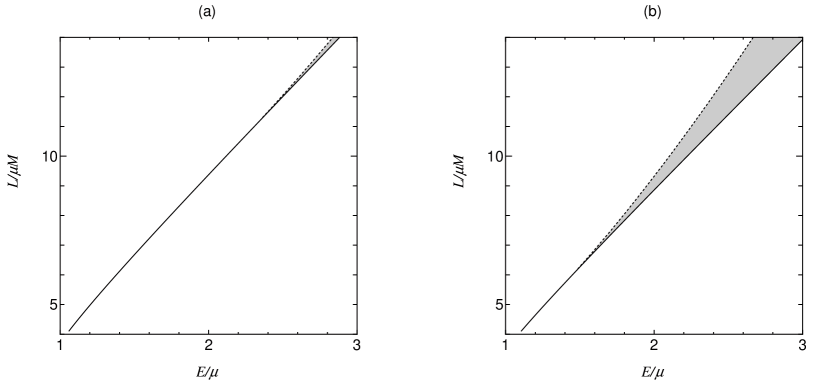
FIG. 1.: Timelike condition for the 4-velocity and the scattered orbit condition for a spinning particle are shown in the case of (a) $S=0.5\mu M$ and (b) $S=0.8\mu M$. The dotted line denotes a null condition, i.e., $v^{\mu}v_{\mu}=0$, and the timelike condition is satisfied in the region above the dotted line. The solid line corresponds to the maximum point of the effective potential $\tilde{V}^{\rm(particle)}$. The shaded region presents a forbidden parameter for a scattered orbit.

FIG. 2.: Location (a) and angular velocity (b) at the turning point of a spinning particle in the case of $R=5.0M$, $E=1.01\mu$, and $L=4.5\mu M$.

]

[

FIG. 3.: Location (a) and angular velocity (b) at the turning point of a spinning particle in the case of $R=2.26M$, $E=2.30\mu$, and $L=12.0\mu M$.

FIG. 4.: Energy spectrum ($l=2$ mode) of gravitational waves from a spinning particle with $E=1.01\mu$ and $L=4.5\mu M$ scattered by a uniform density star with $R=5.0M$. In the parallel case (a), solid, dotted and dashed lines show the case of $S=0$, $0.2\mu M$, and $0.8\mu M$, respectively, while in the anti-parallel case (b), solid, dotted and dashed lines show $S=0$, $-0.2\mu M$, and $-0.8\mu M$. Vertical lines represent the angular velocity of a particle at the turning point.

]

[

FIG. 5.: Total energy of gravitational waves for each multipole mode $l$ in the same situation as Fig. 4. Solid, dotted, dashed, dash-dotted and dash-two dotted lines show the case of $l=2,3,4,5,6$, respectively.

FIG. 6.: Ratio of the total angular momentum to the total energy radiated as gravitational waves for each multipole mode $l$ in the same situation as Fig. 4. Figure (b) is the ratio (a) multiplied by the angular velocity at the turning point for each spin value, in order to estimate Eq. (57). Solid, dotted, dashed, dash-dotted and dash-two dotted lines show the case of $l=2,3,4,5,6$, respectively.

]

[

FIG. 7.: Waveform ($l=2$ mode) of gravitational waves in the direction of $\theta=\pi/2$, $\phi=0$ in the same situation as Fig. 4. In the parallel case (a), solid and dotted lines show the case of $S=0$ and $0.8\mu M$, respectively, while in the anti-parallel case (b), solid and dotted lines show $S=0$ and $-0.8\mu M$.

FIG. 8.: Energy spectrum ($l=2$ mode) of gravitational waves from a spinning particle with $E=1.01\mu$ and $L=4.5\mu M$ scattered by a uniform density star with $R=2.26M$. In the parallel case (a), solid, dotted and dashed lines show the case of the spin $S=0$, $0.2\mu M$, and $0.8\mu M$, respectively, while in the anti-parallel case (b), solid, dotted and dashed lines $S=0$, $-0.2\mu M$, and $-0.8\mu M$. Vertical lines represent the angular velocity of a particle at the turning point. The small figure in (a) and (b) is the enlargement of 1st quasi-normal mode, in order to show the difference of its strength.

]

[

FIG. 9.: Energy spectrum ($l=2$ mode) of gravitational waves from a spinning particle with $E=2.38\mu$ and $L=12.0\mu M$ scattered by the same star as Fig. 8 ($R=2.26M$). In order to focus on the detail of peaks in (a), we show the enlarged figure (b) for the frequency range of $0.0\leq M\omega\leq 0.5$. Solid, dotted and dashed lines show the case of the spin $S=0$, $0.2\mu M$, and $0.8\mu M$, respectively. Vertical lines represent the angular velocity of a particle at the turning point.

FIG. 10.: Location (a) and angular velocity (b) at the turning point of a spinning particle in the case of $R=2.26M$, $E=2.38\mu$, and $L=12.0\mu M$.

]

[

FIG. 11.: Waveform ($l=2$ mode) of gravitational waves in the direction of $\theta=\pi/2$, $\phi=0$ in the same situation as Fig. 9. Solid and dotted lines show the case of the spin $S=0$ and $0.8\mu M$, respectively.

FIG. 12.: Total energy of gravitational waves from a spinning particle with $E=2.30\mu$ and $L=12.0\mu M$ scattered by a uniform density star with $R=2.26M$ for each multipole mode $l$. Solid and dotted lines show the case of $l=2,3$, respectively.

]

[

FIG. 13.: Ratio of the total angular momentum to the total energy radiated $l=2$ gravitational waves in the same situation as Fig. 12.

]

REFERENCES

- [1] K. S. Thorne, in Black Holes and Relativistic Stars, edited by R. M. Wald (University of Chicago Press, Chicago, 1998), p. 41.
- [2] P. Anninos, R. H. Price, J. Pullin, E. Seidel, and W.-M. Suen, Phys. Rev. D 52, 4462 (1995).
- [3] T. Regge and J. A. Wheeler, Phys. Rev. 108, 1063 (1957).
- [4] F. J. Zerilli, Phys. Rev. D 2, 2141 (1970).
- [5] K. S. Thorne and A. Campolattaro, Astrophys. J. 149, 591 (1967); 152, 673 (1967).
- [6] L. Lindblom and S. Detweiler, Astrophys. J. Suppl. Ser. 53, 73 (1983); S. Detweiler and L. Lindblom, Astrophys. J. 292, 12 (1985).
- [7] S. Chandrasekhar and V. Ferrari, Proc. R. Soc. London, Ser. A432, 247 (1991).
- [8] Y. Kojima, Prog. Theor. Phys. 77, 297 (1987).
- [9] A. Borrelli, Nuovo Cimento B 112, 225 (1997).
- [10] K. Tominaga, M. Saijo, and K. Maeda, Phys. Rev. D 60, 024004 (1999).
- [11] Z. Andrade and R. H. Price, Phys. Rev. D 60, 104037.
- [12] V. Ferrari, L. Gualtieri, and A. Borrelli, Phys. Rev. D 59, 124020 (1999).
- [13] J. Ruoff, P. Laguna, and J. Pullin, gr-qc/0005002 (1999).
- [14] V. Ferrari and K. D. Kokkotas, gr-qc/0008057 (2000).
- [15] N. Andersson, Astrophys. J. 502, 708 (1998); J. L. Friedman, and S. M. Morsink, Astrophys. J. 502, 714 (1998).
- [16] B. J. Owen, L. Lindblom, C. Cutler, B. F. Schutz, A. Vecchio, and N. Andersson, Phys. Rev. D58, 084020 (1998).
- [17] D. C. Backer, Astrophys. J. 493, 873 (1998).
- [18] N. Stergioulas and J. L. Friedman, ApJ492, 301 (1998).
- [19] A. Papapetrou, Proc. R. Soc. London A209, 248 (1951).
- [20] W. G. Dixon, in Isolated Gravitating Systems in General Relativity, edited by J. Ehlers (North-Holland, Amsterdam, 1979), p. 156.
- [21] Y. Mino, M. Shibata, and T. Tanaka, Phys. Rev. D 53, 622 (1996); 59, 047502 (1999).
- [22] T. Tanaka, Y. Mino, M. Sasaki, and M. Shibata, Phys. Rev. D 54, 3762 (1996).
- [23] M. Saijo, K. Maeda, M. Shibata, and Y. Mino, Phys. Rev. D 58, 064005 (1998).
- [24] R. Wald, Phys. Rev. D 6, 406 (1972).
- [25] We use a tilde for variables normalized by a particle mass .
- [26] B. S. DeWitt and R. W. Brehme, Ann. Phys. (N.Y.) 9, 220 (1960).
[
]
[
]
[
]
[
]
[
]
[
]
[
]