This thesis is devoted to the study of quantum vacuum effects in the presence of strong gravitational fields. We shall see how the quantum vacuum interacts with black hole geometries and how it can play an important role in the interpretation of the gravitational entropy. In this respect particular attention will be given to the peculiar role of the extremal black hole solutions. From this branch of our research we shall try to collect some important hints about the relation between quantum gravity theories and the semiclassical results. After these investigations we shall move our attention toward possible experimental tests of particle creation from the quantum vacuum which is an indirect confirmation of the Hawking effect. This aim will lead us to study acoustic geometries and their way of “simulating” General Relativity structures, such as horizons and black holes. We shall study the stability of these structures and the problems related to setting up experimental detection of phonon Hawking flux from acoustic horizons. This research will naturally lead us to propose a new model for explaining the emission of light in the phenomenon of Sonoluminescence, based on the dynamical Casimir effect. Possible experimental tests of this proposal will be discussed. In this way we shall set up one of the few available models of quantum vacuum radiation amenable to observational test within the next few years. After this journey in the condensed matter world we shall move to the other arena where our efforts to test the effects of the quantum vacuum in gravitational fields can find a positive solution in the future: the high energy phenomena in the early universe. We shall concentrate our attention on inflation and its possible alternatives for solving the cosmological puzzles. This will lead us to propose a new way to reheat the universe after inflation via pure gravitational effects. We shall finally show how some known phenomena related to the vacuum polarization in the Casimir effects, can naturally suggest new ways to replace (or at least improve) the inflationary scenario.

Notation

Unless otherwise stated we shall use units for which $\hbar=c=1$. We shall make explicit the dependence on the fundamental constants in the most important formulæ. The Boltzmann constant is $k_{\mathrm{B}}$ and the gravitational constant will be denoted as $G_{\mathrm{N}}$. The Greek indices take values $0\dots 3$ while Latin indices denote spatial directions and range over $1\dots 3$.

The wide range of problems treated in this thesis has made it impossible to use the same metric signature through all of the work. Chapters 1 and 4 use the signature common in the literature of quantum field theory $(+,-,-,-)$ with the Minkowski metric given by $\eta_{\mu\nu}={\mathrm{diag}}(1,-1,-1,-1)$. In chapters 2, 3 and 5 we use the signature commonly used by general relativists $(-,+,+,+)$ with the Minkowski metric given by $\eta_{\mu\nu}={\mathrm{diag}}(-1,+1,+1,+1)$.

These notations are consistent with standard reference books in the subject, which have been used as references for the review parts of this work. For purely general relativistic issues we have mainly used references [1, 2, 3], for quantum field theory in external/gravitational fields, the principal sources are [4, 5, 6]. For the review on black hole thermodynamics we have mainly used [3, 7, 8].

The following special symbols and abbreviations are used throughout

$*$	complex conjugate
$\dagger$ or h.c.	Hermitian conjugate
$\partial_{\mu}$ or $\frac{\partial}{\partial x^{\mu}}$ or $\ {}_{,\mu}$	Partial derivative
$\nabla_{\mu}$ or $\ {}_{;\mu}$	Covariant derivative
$\kern 0.5pt{\lower 0.1pt\vbox{\hrule height=0.5pt,width=6.8pt\hbox{\vrule width=0.5pt,height=6.0pt\kern 6.0pt\vrule width=0.3pt} \hrule height=0.3pt,width=6.8pt}}\kern 1.5pt\equiv g^{\mu\nu}\nabla_{\mu}\nabla_{\nu}$	D’Alambertian operator
$\Re$ ($\Im$)	Real (imaginary) part
$\mathrm{Tr}$	Trace
$[A,B]=AB-BA$	Commutator
$\{A,B\}=AB+BA$	Anti-commutator
$\kappa$	surface gravity
$\kappa_{\mathrm{N}}=8\pi G_{\mathrm{N}}$	rescaled Newton constant
$\rho$	mass density
$\varepsilon$	energy density
$r_{\mathrm{h}}$	event horizon radius
${\mathrm{g}}_{\oplus}$	Earth gravity acceleration

Introduction

For most of human history we have searched for our place in the cosmos.

Who are we? What are we?

We find that we inhabit an insignificant planet of a hum-drum star lost in a galaxy

tucked away in some forgotten corner of a universe in which there are far more galaxies than people.

We make our world significant by the courage of our questions, and by the depth of our answers.

Carl Sagan

Among the fundamental forces of nature, gravity still stands in a very particular role. Although the electromagnetic and weak interactions have been successfully unified in the Glashow–Weinberg–Salam model, and the strong force is successfully described with a similar quantum theory, we still lack a quantum description of the gravitational interaction.

The past century has seen a large number of formidable theoretical attacks on the problem of quantum gravity, nevertheless all of these approaches have so far failed (or at the very least proved inconclusive). The reason for such a failure could be just due to the lack of imagination of scientists, but it is beyond doubt that when compared, for example, with quantum electrodynamics, the construction of a quantum theory of gravity turns out to be extremely complicated.

The difficulties on the way to quantum gravity are of different kinds. First of all, the detection of quantum gravitational effects is by itself extremely difficult due to the weakness of the gravitational interaction. In addition one encounters technical problems in quantizing gravity resulting from basic, and peculiar, properties of General Relativity such as the non-linearity of the Einstein equations and the invariance of the theory under the group of diffeomorphisms.

Finally the fact that gravity couples via a dimensional coupling constant $G_{\mathrm{N}}$ makes the theory intrinsically non-renormalizable. For some time it was believed that supergravity theories might overcome this problem, but detailed calculations, and the fact that they are now viewed as effective theories induced from a more fundamental superstring theory, has led to the conclusion that they also suffer with the same problem. Nevertheless one should stress that non-renormalizability of a theory does not necessarily correspond to a loss of meaning.

Nowadays non-renormalizability can be seen as a natural feature of a theory for which the action is not fundamental but arises as an effective action in some energy limit. The Fermi four-fermion model of weak interactions is certainly a non-renormalizable theory but nevertheless it can still be useful in giving meaningful predictions at energies well below those of the $W^{\pm},Z^{0}$ gauge bosons.

In the case of gravity, one may ask when the gravitational interaction can no longer be treated classically. A general dimensional argument is that this happens when the gravitational (Einstein–Hilbert) action is of the same order as the quantum of action $\hbar$

$$S_{\mathrm{grav}}=\frac{c^{3}}{16\pi G_{\mathrm{N}}}\int R\sqrt{g}\;{\mathrm{d}}x\approx\hbar$$ (1)

If $L$ is the typical length scale of the spacetime, one has that the above equality holds for

$$L\approx\sqrt{\frac{\hbar G_{\mathrm{N}}}{c^{3}}}\equiv L_{\mathrm{Pl}}=10^{-33}\,\mbox{cm}$$ (2)

$L_{\mathrm{Pl}}$ is called the Planck length and it corresponds to an energy $E_{\mathrm{Pl}}=c\hbar/L_{\mathrm{Pl}}=\sqrt{\hbar c^{5}/G_{\mathrm{N}}}=10^{19}\,GeV$. Given the fact that the heaviest particles which we are now able to produce are “just” of the order of $TeV=10^{3}\,GeV=10^{-16}\,E_{\mathrm{Pl}}$ (and that the top end of the cosmic ray spectrum is at about $10^{13}\,GeV=10^{-6}\,E_{\mathrm{Pl}}$) it is clear that there is a wide range of energies for which matter can be described quantistically and gravity classically.

This implies that we can limit ourselves to considering theories where quantum fields are quantized in curved backgrounds and where we at most consider the linearized gravitational field (gravitons). In this way the first step of the theory of quantum gravity is naturally the theory of quantum fields (gravitons included) in curved spaces.

Since its first years, this branch of research has focussed particularly on the central role of the quantum vacuum. It was soon discovered that zero point modes of quantum fields are not only influenced by the geometry but are also able to influence gravity in an important way. The theories of black hole evaporation and inflation are nowadays outstanding examples of this.

In this thesis we shall try to present a panoramic view of the general theory of vacuum effects in strong fields, paying special attention to the role of gravity. Our approach will be to focus on different sides of the same physical framework trying to gain new ideas and deeper understanding by a process of developing cross-connections between apparently different physical problems. Sometimes we shall try to learn lessons from our models to then be applied for getting further insight into other different physical phenomena. On other occasions we shall seek experimental tests of theoretical predictions of semiclassical quantum gravity by looking for their analogs in condensed matter physics. Finally we shall also try to gain a deeper understanding of the nature of gravity by considering the possibility of explaining some of its paradoxes by using different paradigms borrowed from our general experience about the dynamics of the quantum vacuum.

Obviously this work is not going to be conclusive but we hope that the reader will be able to see some of the subtle links that connect the theory of semiclassical gravity to a much wider theoretical construction based on the peculiar nature of the quantum vacuum. It is these links which we shall be trying to use for developing new perspectives in this field of research.

Plan of the work

This work is divided into five main chapters. Chapter 1 is devoted to presenting a general view of the main problems and basic ideas of vacuum effects in the presence of external fields with special attention being focussed on the case of gravity.

In chapter 2 we move on to the study of quantum black holes. The thermodynamical behaviour of these objects in the presence of the quantum vacuum will be described and investigated. We shall try to develop the analogy between black hole thermodynamics and the Casimir effect and then we shall investigate the relationship between black hole entropy and the global topology of spacetime. Finally we shall study the nature of extremal black holes.

The following two chapters, chapter 3 and chapter 4, can be seen as two possibly interconnected parallel lines of research, having the common prospect of possibly reproducing some of the most important aspects of semiclassical gravity. The underlying philosophy of these chapters is to investigate the possible use of condensed matter techniques or phenomena to generate laboratory analogs of the phenomenon of particle creation from the quantum vacuum which plays a crucial role in semiclassical gravity.

We shall see in chapter 3 that it may be possible to build up fluid dynamical analogs of the event horizons of general relativity. This research is interesting at different levels. It could in fact give us the possibility to reproduce in the laboratory the most important prediction of semiclassical quantum gravity, the Hawking–Unruh effect. Moreover it can provide us, on the theoretical side, with a deeper understanding of the possible interpretation of General Relativity as an effective theory of gravity.

In chapter 4 we pursue an approach which is the reverse of that in the previous chapter. Instead of trying to build up a condensed matter model reproducing some semiclassical gravity effects, we take a well-known, but unexplained, phenomenon and propose a model based on the production of particles from the quantum vacuum for explaining it. The phenomenon discussed is Sonoluminescence: the emission of visible photons from a pulsating bubble of gas in water.

In chapter 5 we finally move our attention from the realm of condensed matter physics to that of cosmology. This is another promising regime for testing our knowledge of the effects of the quantum vacuum in the presence of strong fields and, in particular, of gravity. Actually cosmology and astrophysics is the only place where we can hope to see the effects of strong gravitational fields in action. We shall discuss some ways in which the quantum vacuum can influence gravitation and be influenced by it, and in particular we study in detail the post-inflationary stage of preheating. At the end of the chapter we discuss the possibility of providing alternatives to the inflationary paradigm and again we shall show that some quantum vacuum effects can play a prominent role also in this case.

This thesis collects results which have been produced in collaboration with several people and which are published in the following papers (listed following the order of appearance in this work) [9, 10, 11, 12, 13, 14, 15, 16, 17, 18, 19, 20, 21]. The research in [22] and [23] will not be presented here because these papers concern issues which are too distant from the main line of this thesis.

Stefano Liberati

Trieste, Italy

April 2000

Chapter 1 Quantum vacuum and Gravitation

If the doors of perception were cleansed

everything would appear as it is,

infinite

William Blake

There is a concept which corrupts and upsets all others.

I refer not to Evil, whose limited realm is that of ethics;

I refer to the infinite.

Jorge Luis Borges

This chapter is an introduction to the issue of the vacuum effects in strong fields. We shall review the basic theory of the quantum vacuum and its application in the presence of external fields. We shall deal with both static and dynamical phenomena and, in connection with the latter, we shall discuss the phenomenon of particle creation from the quantum vacuum due to a strong, time-varying external field. Although most of the chapter is devoted to non gravitational effects, we shall see how most of the concepts introduced here are necessary tools for understanding the physics of a quantum vacuum in gravitational fields. In particular, at the end of this chapter we shall show how the application of such a framework has led to fundamental results in modern theoretical astrophysics.

1.1 The nature of the quantum vacuum

According to Aristotle vacuum is “$\tau\grave{o}\ \kappa\epsilon\nu\acute{o}\nu$”, “the empty”. The same Latin world which we now use, “vacuum”, refers to the absence of anything, to a “space bereft of body”. But what actually is this body?

This apparently easy question has received different answers at different times and these answers often rely on subtle distinctions like, for example, that between matter and what contains it. It is interesting to note that in the last two thousand years both of these concepts have undergone a continuous (and unfinished) evolution in their meaning.

What indeed is matter? The common sense reply (and the one which our ancestors would have given) is that matter is the real substance of which objects are made, and that mass is the concept that quantifies the amount of matter in a body. But it is easy to see how this answer has deeply evolved in time. The famous Einstein formula $E=mc^{2}$ has definitely broken any barrier between matter and energy and nowadays physics assumes the existence (at least in a relative sense) of objects which are never directly subject to our observation.

The concept of space has also changed dramatically. If initially the bodies were located in a Euclidean space, which had its definition in a set of positioning laws, with Newton, Lorentz and Einstein this concept has now evolved. Whereas for Newton “absolute space” was something that “in its own nature, without relation to anything external, remains always similar and immovable”, soon it was recognized that this sort of “stage”, completely independent of matter, was actually only a metaphysical category given the fact that no physical reality can be associated with it. As a consequence mechanics in absolute space and time was replaced in practice by the use of preferred inertial systems e.g. the one defined in terms of the “fixed stars”.

The development of the theory of electromagnetism led later on to the concept of a special ubiquitous medium, the “ether”, in which the electromagnetic waves could propagate, and with Lorentz this ether was described as “the embodiment of a space absolutely at rest”. This concept was also soon rejected when the consequences of Einstein’s theory of Special Relativity were fully understood. Nevertheless Einstein was aware of the fact that his theory did not at all imply the rejection of concepts like empty space; instead he stressed that the main consequence of Special Relativity regarding the ether was to force the discarding of the last property that Lorentz left to it, the immobility. The ether can exist but it must be deprived of any a priori mechanical property. This is actually the main feature that the vacuum (the new name given to the discredited ether) has now in General Relativity. As Einstein himself said “the ether of General Relativity is a medium which by itself is devoid of any mechanical and kinematical property but at the same time determines the mechanical (and electromagnetic) processes”.

In this spirit we now see, via the Einstein equations, not only that the distribution of matter-energy constrains the spacetime itself but also that solutions described by a vacuum (a null stress-energy tensor) are endowed with a complex geometrical structure. In a certain sense we can see now that the synthesis between matter and space, contained and container, is actually achieved in the modern concept of the vacuum which is both.

Still this evolution in the meaning of “the empty” is possibly far from being ended. The development of quantum theory has taught us that the vacuum is not just a passive canvas on which action takes place. It is indeed the most important actor. In modern quantum theories (e.g. string theory) the vacuum has assumed a central role to such an extent that the identification of the vacuum state is the central problem which these have to solve. Particles and matter are merely excitations of the fundamental (vacuum) state and in this sense are just secondary objects.

The phenomena which we are going to discuss are all manifestations of this novel active role of the vacuum in modern physics. We shall see how the vacuum can indeed manifest itself and how it is sensitive to external conditions. As a starting point for our investigation we shall review some basic aspects of the nature of the quantum vacuum in quantum field theory (QFT).

1.1.1 Canonical quantization

Let us consider the standard procedure for second quantization of a scalar field $\phi(t,{\mathbf{x}})$ in Minkowski spacetime. The basic steps required for the quantization are

• Define the Lagrangian or equivalently the equations of motions of the field

  $${\cal L}={\textstyle{1\over 2}}\left(\eta^{\mu\nu}\partial_{\mu}\phi\,\partial_{\nu}\phi-m^{2}\phi^{2}\right)$$ (1.1)

  $$\kern 0.5pt{\lower 0.1pt\vbox{\hrule height=0.5pt,width=6.8pt\hbox{\vrule width=0.5pt,height=6.0pt\kern 6.0pt\vrule width=0.3pt} \hrule height=0.3pt,width=6.8pt}}\kern 1.5pt\phi+m^{2}\phi=0$$ (1.2)

• Define a scalar (aka inner) product

  $$(\phi_{1},\phi_{2})={\mathrm{i}}\int_{\Sigma_{t}}\phi_{1}^{*}\;\stackrel{{\scriptstyle\leftrightarrow}}{{\partial}}_{t}\;\phi_{2}\>{\mathrm{d}}^{3}x,$$ (1.3)

  where $\Sigma_{t}$ denotes a spacelike hyperplane of simultaneity at instant $t$. The value of the inner product has the property of being independent of the choice of $\Sigma_{t}$.

• Find a set of solutions of the field equations $\{\phi^{(+)}_{{\mathbf{k}}}(t,{\mathbf{x}});\phi^{(-)}_{{\mathbf{k}}}(t,{\mathbf{x}})\}$ which is complete and orthonormal with respect to the scalar product just defined $(\phi^{(+)}_{{\mathbf{k}}},\phi^{(-)}_{{\mathbf{k}}})=0$. The superscript $(\pm)$ here denotes solutions with positive and negative energy with respect to $t$.

• Perform a Fourier expansion of the field using the above set

  $$\phi=\sum_{{\mathbf{k}}}\left[a_{{\mathbf{k}}}\phi^{(+)}_{{\mathbf{k}}}(t,{\mathbf{x}})+a^{\dagger}_{{\mathbf{k}}}\phi^{(-)}_{{\mathbf{k}}}\right]$$ (1.4)

  The sum is appropriate for discrete momenta; for continuous ones, an integration is assumed.

• The quantization of the field is carried out by imposing the canonical commutation relations

  $$\left.\begin{array}[]{lll}\left[\phi(t,{\mathbf{x}}),\dot{\phi}(t,{\mathbf{x}}^{\prime})\right]&=&i\hbar c^{2}\delta({\mathbf{x}}-{\mathbf{x}}^{\prime})\\ &&\\ \left[\phi(t,{\mathbf{x}}),\phi(t,{\mathbf{x}}^{\prime})\right]&=&[\dot{\phi}(t,{\mathbf{x}}),\dot{\phi}(t,{\mathbf{x}}^{\prime})]=0\end{array}\right\}$$

  and these imply the commutation relations for the $a_{{\mathbf{k}}},a^{\dagger}_{{\mathbf{k}}}$ coefficients.

  $$\left.\begin{array}[]{lll}\left[a_{{\mathbf{k}}},a^{\dagger}_{{\mathbf{k}}^{\prime}}\right]&=&\delta_{{\mathbf{k}}{\mathbf{k}}^{\prime}}\\ \left[a_{{\mathbf{k}}},a_{{\mathbf{k}}^{\prime}}\right]&=&\left[a^{\dagger}_{{\mathbf{k}}},a^{\dagger}_{{\mathbf{k}}^{\prime}}\right]=0\end{array}\right\}$$ (1.5)

• In the Heisenberg picture, the quantum states span a Hilbert space. A convenient basis in this Hilbert space is the so-called Fock representation. A multiparticle state $|n_{{\mathbf{k}}}\rangle$ can be constructed from the special state $|0\rangle$ by the application the coefficients defined above. The coefficients $a_{{\mathbf{k}}},a^{\dagger}_{{\mathbf{k}}}$ become, via the relations (1.5), operators respectively of destruction and creation of one particle of momentum ${\mathbf{k}}$.

  $$a^{\dagger}_{{\mathbf{k}}}\,|n_{{\mathbf{k}}}\rangle=\sqrt{n+1}\,|(n+1)_{{\mathbf{k}}}\rangle$$ (1.6)

  $$a_{{\mathbf{k}}}\,|n_{{\mathbf{k}}}\rangle=\sqrt{n}\,|(n-1)_{{\mathbf{k}}}\rangle$$ (1.7)

  the vacuum state $|0\rangle$ is defined as the state that is annihilated by the destruction operator for any ${\mathbf{k}}$

  $$a_{{\mathbf{k}}}|0\rangle\equiv 0\qquad\forall{\mathbf{k}}$$ (1.8)

• If we now consider the bilinear operator $N_{{\mathbf{k}}}\equiv a_{{\mathbf{k}}}^{\dagger}a_{{\mathbf{k}}}$ then its expectation value on the vacuum state and on a multiparticle state are respectively

  $$\langle 0|N_{{\mathbf{k}}}|0\rangle=0\qquad\forall{\mathbf{k}}$$ (1.9)

  $$\langle n|N_{{\mathbf{k}}}|n\rangle=n_{{\mathbf{k}}}$$ (1.10)

  Thus the expectation value of the operator $N_{k}$ tells us the number of particles with momentum ${\mathbf{k}}$ in a given state. The vacuum state is in this sense the only state which has no particles for any value of ${\mathbf{k}}$.

The above considerations are all based on the definition of some complete orthonormal set of classical solutions $\phi^{(+)}_{{\mathbf{k}}}(t,{\mathbf{x}});\phi^{(-)}_{{\mathbf{k}}}(t,{\mathbf{x}})$. In the absence of external fields and in Minkowski space the eigenfunctions of the translation in time operator $\partial/\partial t$, which is the generator of the Poincaré group, form a privileged set of such solutions (the set associated with inertial observers). In this case the $\phi^{(+)}$ and $\phi^{(-)}$ have a clear meaning of positive and negative frequency solutions and the vacuum state $|0\rangle$ defined via Eq. (1.8) is invariant under transformations of the Poincaré group. So the procedure for constructing the Fock space turns out to be completely unambiguous.

1.1.2 Canonical quantization in external fields

The situation is completely different when the quantization has to be carried out in the presence of an external field. By “external” we mean that the field, which interacts with the one which we want to quantize, is introduced at a classical level and is not itself a dynamical variable. We shall see that the role of external field can be played by very different objects such as electromagnetic and gravitational fields, some geometrical boundary of the spacetime or some non trivial topology of the manifold over which the quantization is performed. Different phenomenologies are also going to be encountered depending on whether the external field is stationary or not. If it is stationary, one generically expects vacuum polarization effects, while if it is not stationary, there can be particle emission from the quantum vacuum.

In the presence of an external field the translation invariance in time or space is broken and it is hence impossible to uniquely define an orthonormal basis. Different complete orthonormal sets of solutions become equally valid but they lead to different inequivalent vacua. The basic point is that in this situation the Poincaré group is no longer a symmetry group of the spacetime (e.g. because this is curved or characterized by boundaries) and hence the vacuum state $|0\rangle$ defined via Eq. (1.8) is now generally dependent on the basis used for performing the quantization.

In the case that the external field is a gravitational one, the best thing that one can hope to do is to look for timelike Killing vectors to use for properly defining the decomposition into positive and negative energy frequency modes. In some simple cases the global structure of the spacetime is asymptotically Minkowskian and hence it is possible to have a natural reference vacuum to use in defining the particle content of the other vacua allowed by the equivalent sets of orthonormal bases. We shall come back to this issue later on.

In the next section we shall illustrate a useful technique which allows inequivalent vacua to be related via a conceptually easy formalism. This technique, generally referred to as a “Bogoliubov transformation”, will be used several times in the body of this thesis.

Bogoliubov transformation

We can start by considering the case of a scalar field which is quantized in the presence of an external field (which can be gravitational or not, static or dynamically changing in time). Imagine that the problem admits at least two distinct complete orthonormal sets of modes as solutions of the equations of motion of the field. In what follows we shall see similar situations in the case of time varying external fields or in the case of a static spacetime which admits two different global Killing vectors associated with isometries in time (and hence two distinct ways to define positive frequency modes).

In any case, the above statement implies that it is possible to decompose the field $\phi$ in two different ways

$$\phi(t,{\mathbf{x}}) = \sum_{i}\left(a_{i}\varphi_{i}(t,{\mathbf{x}})+a^{\dagger}_{i}\varphi^{*}_{i}(t,{\mathbf{x}})\right)$$ (1.11)

$$\phi(t,{\mathbf{x}}) = \sum_{j}\left(b_{j}\psi_{j}(t,{\mathbf{x}})+b^{\dagger}_{j}\psi^{*}_{j}(t,{\mathbf{x}})\right)$$ (1.12)

where $i$ and $j$ schematically represent the sets of quantities necessary to label the modes.

These two decompositions will correspond to two inequivalent vacua defined respectively as

$$|0\rangle_{\varphi} a_{i}|0\rangle_{\varphi}\equiv 0$$ (1.13)

$$|0\rangle_{\psi} b_{j}|0\rangle_{\psi}\equiv 0$$ (1.14)

The completeness of both sets allows one to be expanded as a function of the other

$$\varphi_{i} = \sum_{j}\left(\alpha_{ij}\psi_{j}+\beta_{ij}\psi^{*}_{j}\right)$$ (1.15)

$$\psi_{j} = \sum_{i}\left(\alpha^{*}_{ij}\varphi_{i}-\beta_{ij}\varphi^{*}_{i}\right)$$ (1.16)

These relations are called Bogoliubov transformations and the $\alpha$ and $\beta$ coefficients are called Bogoliubov coefficients. The latter are easily calculated via the inner product (1.3) as

$$\alpha_{ij}=-(\psi_{i},\varphi_{j}),\qquad\beta_{ij}=(\varphi^{*}_{i},\psi_{j})$$ (1.17)

From the equivalence of the mode expansions and using (1.15) together with the orthogonality of the modes, it is possible to relate the creation and destruction coefficients of the two bases:

$$a_{i} = \sum_{j}\left(\alpha^{*}_{ij}b_{j}-\beta^{*}_{ij}b^{\dagger}_{j}\right)$$ (1.18)

$$b_{j} = \sum_{i}\left(\alpha_{ji}a_{i}+\beta^{*}_{ji}a^{\dagger}_{i}\right)$$ (1.19)

From the above relations it is easy to show that the Bogoliubov coefficients must satisfy the following properties

$$\sum_{k}\left(\alpha_{ik}\alpha^{*}_{jk}-\beta_{ik}\beta^{*}_{jk}\right) = \delta_{ij}$$ (1.20)

$$\sum_{k}\left(\alpha_{ik}\beta_{jk}-\beta_{ik}\alpha_{jk}\right) = 0$$ (1.21)

Now it is clear, from the relation (1.18) between the destruction operators in the two bases, that the two vacuum states associated with the two choices of the modes $\varphi_{i}$ and $\psi_{j}$, are different only if $\beta_{ij}\neq 0$. In fact in this case one finds that the vacuum state $|0\rangle_{\psi}$ will not be annihilated by the destruction operator of the $\varphi$ related basis

$$a_{i}|0\rangle_{\psi}=\sum_{j}\beta^{*}_{ij}|1_{j}\rangle_{\psi}\neq 0$$ (1.22)

Actually, if we look at the expectation value of the operator, $N_{i}=a^{\dagger}_{i}a_{i}$, for the number of $\varphi_{i}$-mode particles in the vacuum state of the $\psi_{j}$ modes, we get

$$\langle 0|N_{i}|0\rangle_{\psi}=\sum_{j}|\beta_{ji}|^{2}$$ (1.23)

This is equivalent to saying that the vacuum of the $\psi$ modes contains a non null number of particles of the $\varphi$ mode.

It is then clear that the notion of a particle becomes ambiguous in these situations as a consequence of the ambiguity in the definition of the vacuum state. To obtain a more objective qualification of the state of the field one should refer to objects which are covariant locally defined quantities such as the expectation value of the stress energy tensor.

In this sense it is important to recall that the stress energy tensor (SET) of the field can be cast in a form where an explicit dependence on $\beta^{2}$ appears. Nevertheless one can see the it will generally depend also on “interference” terms of the kind $\alpha\beta$ [53]. This is symptomatic of the looseness of the relation between particles and energy-momentum. We shall directly experience this feature in the next chapter when we discuss particle creation by collapsing extremal black holes in section 2.5.

Another important point which we want to stress here is that the Bogoliubov coefficients are just telling us the relation between vacuum states. In the case in which the two distinct sets of normal modes correspond to two asymptotic states in time (for example in the case in which the external field is static, then changes its value, then is again static) this relation is interpreted as particle creation. If the $\psi$ modes are appropriate at early times and the $\varphi$ ones are appropriate at late times, then the relation (1.23) can be interpreted as saying that the $|0\rangle_{\psi}$ has evolved into the $|0\rangle_{\varphi}$ plus some particles.

Although the Bogoliubov transformation technique has often been used for describing particle creation by nonstationary external fields it should be stressed that the information which one can actually get from the value of the coefficients is limited. The relation (1.23) should more correctly be interpreted in the sense of a “potential possibility”, it tells us that the $\psi$ state is potentially equivalent to the $\varphi$ state plus some $\varphi$-particles. It does not give a priori any information about the actual timing of the emission (when the particles are effectively produced). This information requires the study of other quantities such as the stress-energy tensor.

Comment: The inner product (1.3) is by construction independent of the chosen $t=\mbox{constant}$ hypersurface. This implies that in the case considered above, when one has only two sets of basis states, also the Bogoliubov coefficients (1.17) will be time independent. It is nevertheless possible to have more complex situations where one has more, time dependent, bases of states. In these cases one has to build up the Bogoliubov coefficients by taking the inner product between some initial basis and a time-dependent “instantaneous” one. It is clear that in such circumstances the Bogoliubov coefficients will indeed depend on time. We shall discuss the instantaneous basis formalism in section 1.3.1.

1.1.3 The quantum vacuum

The concept of the vacuum being a dynamical object endowed with an autonomous existence is clearly shown in the framework discussed above. In fact it is a postulate of QFT that, when a measurement of a physical quantity is performed, the quantum system is compelled to occupy an eigenstate of the operator corresponding to the physical quantity concerned. Since non commuting operators do not share common eigenstates, this implies that if a system is in an eigenstate of a given operator then, in general, it will not posses the properties described by other operators which do not commute with the given one.

We have seen that the vacuum state is an eigenstate with zero eigenvalue of the particle number operator $N_{{\mathbf{k}}}$ so in this state it makes no sense to discuss the properties described by operators which do not commute with $N_{{\mathbf{k}}}$ such as the field operator or the current density. Moreover, there cannot exist any state which is an eigenstate of both $N_{{\mathbf{k}}}$ and any of the other non commuting operators. In the same way that in quantum mechanics it is impossible for a particle to have zero values of both the coordinate and the momentum, also in QFT it is impossible to find a state in which there are simultaneously no photons and no quantized electromagnetic field (virtual photons) or electrons and no electron-positron current. There is never a truly “empty” vacuum state.

A crucial feature of the quantum vacuum, which is important for our future discussion, is the fact that it is not only ubiquitous but at the same time it appears to be endowed with an infinite energy. If we consider the stress energy tensor of a free scalar field in flat space

$$T_{\mu\nu}=\partial_{\mu}\phi\,\partial_{\nu}\phi-{\textstyle{1\over 2}}\eta_{\mu\nu}\eta^{\lambda\delta}\partial_{\lambda}\phi\,\partial_{\delta}\phi+{\textstyle{1\over 2}}m^{2}\phi^{2}\eta_{\mu\nu}$$ (1.24)

then it is easy to calculate the Hamiltonian and the Momentum and express them in terms of the creation and destruction operators (using the expansion of the field)

$${\cal H} = \int_{t}{T_{00}{\mathrm{d}}^{3}x=\sum_{{\mathbf{k}}}\omega_{{\mathbf{k}}}\left(a^{\dagger}_{{\mathbf{k}}}a_{{\mathbf{k}}}+\frac{1}{2}\right)}$$ (1.25)

$${\cal P} = \int_{t}{T_{0i}{\mathrm{d}}^{3}x=\sum_{{\mathbf{k}}}a^{\dagger}_{{\mathbf{k}}}a_{{\mathbf{k}}}\,k_{i}}$$ (1.26)

We can now look at the vacuum expectation values of these operators. Although the momentum gives the expected vanishing value

$$\langle 0|{\cal P}|0\rangle=0$$ (1.27)

the expectation value of the Hamiltonian, the vacuum energy, clearly shows a divergence

$$\langle 0|{\cal H}|0\rangle={1\over 2}\sum_{{\mathbf{k}}}\omega_{{\mathbf{k}}}=\infty$$ (1.28)

This divergence of the vacuum energy can be shown to be generic; nevertheless in Minkowski spacetime it can be removed by the introduction of “normal ordering”. This is generally denoted by :: and demands that in any product of creation and annihilation operators, the latter should be on the right of the former. Implicitly this is equivalent to setting the energy of the Minkowski vacuum to zero, the only justification for this assumption being “outside” of QFT actually in the fact that Minkowski vacuum does not appear to gravitate — flat spacetime is a solution of the Einstein equations where the expectation value of the stress energy tensor is zero everywhere.

In the case of quantization in curved spacetimes or in the presence of external fields or boundaries, that is in all the cases where the central role of the Poincaré group breaks down, we do not have a general way to specify a privileged vacuum and hence a normal ordering procedure. Although this can generically lead to an intrinsic ambiguity of the canonical quantization in external fields it is again true that in a large class of cases an asymptotic symmetry group exists which allows meaningful construction of a reference vacuum for the specific physical problem which one wants to solve.

The relevance of the identification of such a reference background is again important because it allows “rescaling” of the energy of the (divergent) vacuum in the presence of some external field $\lambda$ by subtracting the (divergent) energy of the asymptotic one (where the external field has an asymptotic, possibly vanishing, value $\lambda_{0}$).

$$E_{\mathrm{phys}}=E[\lambda]-E[\lambda_{0}]$$ (1.29)

One may wonder why we could not always try to rescale the vacuum energy in such a way as to make it zero. The point is that also in this case we would not be allowed to discard the existence of the vacuum, in fact the expectation value of the fluctuations of the fields would still be non-zero in the vacuum.

$$\Delta(\phi^{2}(t,{\mathbf{x}}))=\langle 0|\phi^{2}(t,{\mathbf{x}})|0\rangle-\langle 0|\phi(t,{\mathbf{x}})|0\rangle^{2}$$ (1.30)

Of course the above mentioned removal of divergences generally implies the use of regularization procedures and renormalizations of the stress energy tensor. In these procedures there are inherent pitfalls and difficulties. Most of these are mainly related to the fact that while the renormalization procedure should obviously be covariant and gauge invariant, at the same time the presence of external conditions require the use of both a definite coordinate system and a specific gauge for the external field. We shall not deal with these technical issues here and direct the reader to standard textbooks [4, 5, 6]. We shall see this framework in action several times in this thesis.

As a related remark we would like to make clear why such a heuristic procedure as the one described above, is generically able to remove the divergences from the vacuum energies. The basic point here is that the divergences of the kind shown in Eq. (1.28) are clearly of ultraviolet nature. They came from the behaviour of the quantum field theory at extremely short scales. On the other hand the external fields generally determine a change in the vacuum structure at a global level. This implies a universal nature for the vacuum divergences and gives a concrete explanation for the cancellation of the divergent part of the vacuum energies.

Now that we have sketched how there can be finite differences in vacuum energy it is natural to ask if such energies are indeed physically relevant and observable. In the next section we shall discuss some examples in which the “external field” is static and lead just to a change in the vacuum energy and we shall see how these energy shifts actually lead to observable forces. After this we shall discuss the influence of nonstationary external fields and their ability to lead to particle creation from the quantum vacuum. At the end, we shall deal specifically with vacuum effects in gravitational fields.

Comment: Although one can be tempted to link concepts like vacuum energy shifts and particle creation respectively to effects in static and dynamical external fields, it has to be stressed that such a sharp distinction cannot exist. For example a static electric field can create electron-positron pairs and a nonstationary electromagnetic field can polarize the vacuum without relevant particle production. The very concept of a distinction between vacuum polarization and particle production can be subtle and needs to be handled with caution.

1.2 Vacuum effects in static external fields

In this section we consider a special class of quantum vacuum effects induced by static external fields. This last phrasing is generally used in the literature to cover a wide range of possibilities. It can be used for vacuum effects in the presence of boundaries but also for those induced by quantization on spaces with non trivial topologies (in flat as well as in curved backgrounds). Of course there are also cases in which the external field is truly a classical field, for example it can be a scalar, electromagnetic or gravitational field.

Here we shall give a brief presentation of only the first two kinds of effect (those induced by boundaries and topology). Particular attention will be given to the case of the gravitational field in the last section of this chapter where we shall treat static as well as dynamical cases.

1.2.1 The Casimir effect

In 19th century P.C. Causseè described in his “L’ Album du Marin” a mysterious phenomenon which was the cause of maritime disasters [24, 25]. Figure 1.1 shows the situation which he called “Calme avec grosse houle”: no wind but still with a big swell running. In this situation he stressed that if two ships end up lying parallel at a close distance then often “une certaine force attractive” was appearing, pulling the two ships towards each other and possibly leading to a collision.

Figure 1.1: From Causseè “The Mariners Album”, two ships heavily rolling in a situation where there are still long waves but no wind.

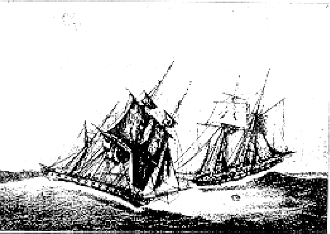
This phenomenon was for many years considered as just another superstition of sailors because it was far from clear what force should be at work in these situations. It is only recently that this effect was given the name of the “Maritime Casimir Effect” [25].

We shall not discuss here in detail the explanation proposed in [25] but limit ourselves to a heuristic explanation that will be useful as an introduction to the real Casimir effect .

Following the discussion of the previous section we can start by looking at the configuration characterized by just open sea. In this case the background is characterized by arbitrarily long waves. Let us concentrate on the direction orthogonal to the alignment of the boats. This is the only direction, say the $x$ direction, which is affected by the location of the ships.

The waves in the open sea can have wavelengths $\lambda$ covering the whole range of $x$, and so their wave number $k=2\pi/\lambda$ runs over a continuous range of values.

When the ships are introduced, the $x$ direction automatically acquires a scale of length and the waves between the two boats are now obliged to have wave numbers which are integer multiples of a fundamental mode inversely proportional to the distance $a$ between the ships, $k_{n}=\pi n/a$.

The energy per mode will obviously be changed, nevertheless the total energy will in both cases be infinite (being given by the sum over the modes). What indeed can be expected is that the regularized total energy in the case of the two ships is less than the corresponding one for the open sea. In fact just a discrete (although still infinite) set of waves will be allowed leading to a negative result when performing the subtraction (1.29).

A negative energy density then automatically leads to an attractive force between the two ships. Although this maritime Casimir effect can be see as a nice macroscopic example of the quantum effect which we are going to treat in detail, it should be stressed that it cannot be more than an analogy; actually it is impossible that for two aligned boats in an open sea there could be an accurate description of their attraction in the above terms: other effects of many sorts will influence the behaviour of the ships and make any interpretation of the observations obscure. All in all, we are not sure that Mr. Causseè was not telling us one of the numerous mariners stories …

A 1+1 version of the Casimir effect

In 1948 the Dutch physicist H.B.G Casimir predicted that two parallel, neutral, conducting plates in a vacuum environment should attract each other by a very weak force per unit area that varies as the inverse forth power of their separation [26],

$$F=-\frac{\pi^{2}}{240}\frac{\hbar c}{a^{4}}$$ (1.31)

This effect was experimentally confirmed in the Philips laboratories [27] a decade later (see also [28, 29] for more recent results). For plates of area $1\ {\rm cm}^{2}$ and separation of about half a micron the force was $\approx 0.2\cdot 10^{-5}$ N in agreement with the theory.

To be concrete we shall now show a simplified calculation of the Casimir effect made using a massless scalar field and working in 1+1 dimensions .

The 1+1 Klein-Gordon equation takes the form

$$\kern 0.5pt{\lower 0.1pt\vbox{\hrule height=0.5pt,width=6.8pt\hbox{\vrule width=0.5pt,height=6.0pt\kern 6.0pt\vrule width=0.3pt} \hrule height=0.3pt,width=6.8pt}}\kern 1.5pt\phi(t,x)=0$$ (1.32)

We shall assume the internal product and canonical commutation relations as given in equations (1.3) and (• ‣ 1.1.1) and a standard quantization procedure as previously discussed in section 1.1.1. Generically the solutions of the equation of motion can be expressed in the form of traveling waves:

$$\phi_{k}^{(\pm)}(t,x)=\frac{\textstyle 1}{\textstyle\sqrt{4\pi\omega}}\exp[\pm{\mathrm{i}}(\omega t-kx)]$$ (1.33)

$$\omega^{2}=k^{2},\qquad-\infty<k<+\infty$$

We can now consider the one dimensional analogue of the Casimir effect, that is a boundary in the $x$ direction that imposes Dirichlet boundary conditions on the field.

$$\phi(t,0)=\phi(t,a)=0$$ (1.34)

In this case we have again that there is a discrete set of allowed wavenumbers and that the wavefunctions are of the form

$$\phi_{k}^{(\pm)}(t,x)=\frac{\textstyle 1}{\textstyle\sqrt{a\omega_{n}}}\exp[\pm{\mathrm{i}}(\omega_{n}t)]\sin{k_{n}x}$$ (1.35)

$$\omega^{2}=k^{2}_{n},\qquad k_{n}=\pi n/a\quad n=1,2,\dots$$

From the above forms of the normal modes it is clear that the creation and destruction coefficients will be different in the two configurations (free and bounded space) and hence the vacuum states, $|0\rangle_{\mathrm{Mink}}$ and $|0\rangle$, will differ as well.

Using the fact that the Hamiltonian of the field has the form (1.25) we can find the expectation value of the field energy in the vacuum state for the two configurations (free and bounded)

$$E_{\mathrm{free}} = \langle 0|{\cal H}|0\rangle_{\mathrm{Mink}}={\textstyle{1\over 2}}\int_{-\infty}^{+\infty}{\frac{\textstyle{\mathrm{d}}k}{\textstyle 2\pi}|k|L}$$ (1.36)

$$E_{\mathrm{bound}} = \langle 0|{\cal H}|0\rangle={\textstyle{1\over 2}}\sum_{n=1}^{\infty}{\frac{\textstyle\pi n}{\textstyle a}}$$ (1.37)

where we have introduced in (1.36) a normalization length $L\to\infty$.

Both of the above quantities are divergent so, in order to compute them and correctly execute the “Casimir subtraction” (1.29) we should adopt some regularization scheme.

This can be done using an exponential cutoff of the kind $\exp{(-\alpha\omega)}$ and by looking in the Minkowskian case at the energy in a region of length $a$. To compute this last quantity we shall look at the energy density $E_{\mathrm{free}}/L$ times $a$. The results are then

$$E_{\mathrm{free}}^{a} = \frac{E_{\mathrm{free}}\cdot a}{L}={\textstyle{1\over 2}}\int_{-\infty}^{\infty}{{\mathrm{d}}k|k|a\,\exp{(-\alpha|k|)}}=\frac{\textstyle a}{\textstyle 2\pi\alpha^{2}}$$ (1.38)

$$E_{\mathrm{bound}} = {\textstyle{1\over 2}}\sum_{n=1}^{\infty}\frac{\textstyle\pi n}{\textstyle a}\exp{(-\alpha\pi n/a)}=\frac{\textstyle a}{2\pi\alpha^{2}}-\frac{\textstyle\pi}{24a}+O(\alpha^{2})$$ (1.39)

So we see that in the limit $\alpha\to\infty$ the subtraction $E_{\mathrm{bound}}-E_{\mathrm{free}}^{a}$ gives a finite quantity $E_{\mathrm{Casimir}}=-\pi/(24a)$ to which corresponds to an attractive force

$$F_{\mathrm{Casimir}}=-\frac{\partial E_{\mathrm{Casimir}}}{\partial a}=-\frac{\pi}{24a^{2}}$$ (1.40)

The true Casimir calculation, performed in three spatial dimensions and with the electromagnetic field, has the same functional form. It actually differs from the one found above in the value of the numerical prefactor and in the power of the typical length scale (a clear consequence of the different number of dimensions).

The calculation just sketched has been performed for different geometrical configurations and notably it turns out that the value and even the sign of the Casimir energy is a non trivial function of the chosen geometry. In particular it is interesting to note that the Casimir energy in a cubic cavity is negative but that in a spherical box turns out to be positive.

There are some important points that have to be stressed before proceeding.

1. The Casimir effect could be interpreted as a manifestation of van der Waals forces of molecular attraction. However the force (1.31) has the property of being absolutely independent of the details of the material forming the conducting plates. This is a crucial feature which establishes the definitive universal nature of the Casimir effect. The independence from the microscopic structure of the plates proves that the effect is just a byproduct of the nature of the quantum vacuum and of the global structure of the manifold.

2. The fact that for different geometries also positive energy densities can be obtained implies that the heuristic interpretation, that the presence of the boundaries “takes away” some modes and hence leads to a decrement of the total energy density with respect to the unbound vacuum, is wrong. What actually happens is that the number of modes allowed between the (ideal) plates is still infinite, what changes is the distribution of the vacuum field modes. What we see as the appearance of a repulsive or attractive vacuum pressure is an effect of this (geometry dependent) redistribution of modes [33].

3. A common terminology used for describing the shift in the vacuum energy appearing in static Casimir effects is that of “vacuum polarization”. The vacuum is described as a sort of dielectric material in which at small distances virtual particle-antiparticle pairs are present, analogously to the bounded charges in dielectrics. The presence of boundaries or external forces “polarizes” the vacuum by distorting the virtual particle-antiparticle pairs. If the force is strong enough it can eventually break the pairs and “the bound charges of the vacuum dielectric” become free.

   Although this has turned out to be a useful concept, at the same time it should be stressed that it is strictly speaking incorrect. The vacuum state is an eigenstate of the number operator which is a global operator (because it is defined by the integral of the particle density over the whole 3-space). On the other hand, the field operator, the current density and the other typical operators describing the presence of particles are local, so there is a sort of complementarity between the observation of a (global) vacuum state and (local) particle-antiparticle pairs.

   In the following we shall use this standard terminology but keeping in mind the fact that it is a misuse of language.

Finally I would like to point out an important feature common to a wide class of cases of vacuum polarization in external fields. We can return to our example of $1+1$ Casimir effect. Consider the energy density which in this case is simply given by Eq.(1.37) divided by the interval length $a$.

$$\varepsilon=\langle 0|T_{00}|0\rangle=\frac{1}{2a}\sum_{n=1}^{\infty}\omega_{n}\,,\qquad\omega_{n}=\frac{\pi n}{a}$$ (1.41)

In order to compute it we can adopt a slightly different procedure for making the Casimir subtraction. It is in fact sometimes very useful in two dimensional problems to use (especially for problems much more complicated that the one at hand) the so called Abel–Plana formula which is generically

$$\sum_{n=0}^{\infty}F(n)-\int_{0}^{\infty}F(\sigma){\mathrm{d}}\sigma=\frac{F(0)}{2}+{\mathrm{i}}\int_{0}^{\infty}{\mathrm{d}}\sigma\frac{F({\mathrm{i}}\sigma)-F(-{\mathrm{i}}\sigma)}{\exp{(2\pi\sigma)}-1}\equiv{\mathrm{reg}}\sum_{0}^{\infty}F(n)$$ (1.42)

where $F(z)$ is an analytic function at integer points and $\sigma$ is a dimensionless variable. This formula is a powerful tool in calculating spectra because the exponentially fast convergence of the integral in $F(\pm{\mathrm{i}}\sigma)$ removes the need for explicitly inserting a cut-off.

In our specific case, $F(n)=\omega_{n}$, and so Eq.(1.42) applied to the former energy density takes the form

$$\varepsilon_{\rm ren}=-\frac{1}{\pi}\int_{0}^{\infty}\frac{\omega{\mathrm{d}}\omega}{\exp{(2a\omega)}-1}$$ (1.43)

Although it may appear surprising, we have found that the spectral density of the Casimir energy of a scalar field on a line interval does indeed coincide, apart from the sign, with a thermal spectral density at temperature $T=1/a$.

The appearance of the above “thermality” in the static Casimir effect is not limited to the case of external fields implemented via boundary conditions and it is not linked to the use of the Abel–Plana formula (which is merely a computational tool). As we shall see, it can appear also when quantization is performed in the presence of a gravitational field (in the case of spacetimes with Killing horizons). We shall try to give further insight on this point later on in this chapter.

Before considering other examples of vacuum polarization we shall now devote some words to an interesting effect which is related to the Casimir one.

The Scharnhorst effect

In 1990 K. Scharnhorst and G. Barton [34, 35, 36] showed that the propagation of light between two parallel plates is anomalous and indeed photons propagating in directions orthonormal to the plates appear to travel at a speed $c_{\bot}$ which exceeds the speed of light $c$. The propagation of photons parallel to the Casimir plates is instead at speed $c_{\|}=c$.

The above results where found starting from the Maxwell Lagrangian modified via a non-linear term stemming from the energy shifts in the Dirac sea induced by the electromagnetic fields. The action obtained in this way is the well known Euler–Heisenberg one which in its real part takes the form ($m_{e}$ is the electron mass)

$${\cal L}=\frac{{\mathbf{E}}^{2}-{\mathbf{B}}^{2}}{8\pi}+\frac{\alpha^{2}}{2^{3}\cdot 3^{2}\cdot 5\pi^{2}m_{e}^{4}}\left[\left({\mathbf{E}}^{2}-{\mathbf{B}}^{2}\right)^{2}+7\left({\mathbf{E}}\cdot{\mathbf{B}}\right)\right]$$ (1.44)

One can see here that the correction is proportional to the square of the fine structure constant and so it is a one-loop effect.

The above action in particular also describes the scattering of light by light and can be read as giving to the vacuum an effective, intensity-proportional, refractive index $n=1+\Delta n$. The Scharnhorst effect can be seen as a consequence of the fact that in the Casimir effect the intensity of the zero-point modes is less than in unbounded space and hence leads to a proportionate drop in the effective refractive index of the vacuum ($\Delta n<0$).

It should be stressed that the above results are frequency independent for $\omega\ll m$ and so the phase, group and signal velocities coincide. Moreover using the Kramers–Kronig dispersion relation

$$\Re\left\{n(\omega)\right\}=\Re\left\{n(\infty)\right\}+\frac{2}{\pi}\int_{0}^{\infty}{\mathrm{d}}\omega^{\prime}\;\frac{\omega^{\prime}\Im\left\{n(\omega^{\prime})\right\}}{{\omega^{\prime}}^{2}-\omega^{2}}$$ (1.45)

and assuming that the vacuum always acts a passive medium ($\Im\left\{n(\omega)\right\}\geq 0$), it has been shown [36] that the effective refractive index of the vacuum at high frequencies must be smaller than that at low frequencies, and so

$$1>n_{\bot}(0)\geq n(\infty)$$ (1.46)

Although this anomalous propagation is too small to be experimentally detected (the corrections to the speed of light are of order $\alpha^{2}/(md)^{4}$, where $d$ is the distance between the plates) it is nevertheless an important point that a vacuum which is polarized by an external field can actually behave as a dispersive medium with refractive index $n(\omega)$ less than one. In fact similar effects have been discovered in the case of vacuum polarization in gravitational fields [37, 38, 39, 40].

This realization has important consequences and deep implications (e.g. about the meaning of Lorentz invariance and the possible appearance of causal pathologies [41]) which are beyond the scope of the present discussion. We just limit ourselves to noting the fact that these issues can be dealt with very efficiently in a geometric formalism where the modification of the photon propagation can be “encoded” in an effective photon metric $g_{\mu\nu}^{\mathrm{eff}}$ [42, 43, 44]. In particular, in [43] it is shown that in a general non linear theory of electrodynamics, this effective metric can be related to the Minkowski metric via the renormalized stress-energy tensor, in the form

$$g^{\mathrm{eff}}_{\mu\nu}=A\eta_{\mu\nu}+B\langle T_{\mu\nu}\rangle$$ (1.47)

where $A$ and $B$ are constants depending on the specific form of the Lagrangian.

We shall see in chapter 5 (section 5.6) how this relation generalizes in curved spacetimes and what its possible role can be in modern cosmology. For the moment, we shall return to our general discussion of vacuum effects in static external fields.

1.2.2 Other cases of vacuum polarization

The Casimir effect which we have been discussing is just a special case of a more general class of phenomena leading to vacuum polarization via some special boundary conditions that makes the quantization manifold different from the Minkowskian one. Generally speaking, this class is divided into effects due to physical boundaries (which are strictly the Casimir effects) and those due to nontrivial topology of the spacetime (which are generally called topological Casimir effects).

We have briefly discussed some cases of the first class: in general they are all variations on the main theme of the Casimir effect. They are all in Minkowski space with some boundary structure, all that changes is the kind of field quantized, the geometry of the boundaries (parallel plates, cubes, spheres, ellipsoids etc.) and the number of spatial dimensions.

In the second class of phenomena, the quantization is performed in flat spacetimes (or curved ones, as we shall see later) endowed with a non trivial topology (that is with a topology different from the standard $R\times R^{3}$ of Minkowski spacetime). The topology is generally reflected in periodic or anti-periodic conditions on the fields. Again the trivial example of the quantization of a scalar field on the interval $(0,a)$ turns out to be useful.

Let us consider the case of periodic boundary conditions:

$$\phi(t,0)=\phi(t,a)$$ (1.48)

$$\partial_{x}\phi(t,0)=\partial_{x}\phi(t,a)$$ (1.49)

This time, in the points $x=0,a$ we are allowed to have also non-zero modes, and hence we shall have, as possible solutions, the one in Eq.(1.35) and another one with $\cos k_{n}x$ replacing the sine. Hence, we get a doubled number of modes and a different spectrum:

$$\phi_{k}^{(\pm)}(t,x)=\frac{\textstyle 1}{\sqrt{\textstyle 2a\omega_{n}}}\exp[\pm{\mathrm{i}}(\omega_{n}t-k_{n}x)]$$ (1.50)

$$\omega^{2}=k^{2}_{n},\qquad k_{n}=2\pi n/a\quad-\infty<n<\infty$$

The unbounded space solutions will still be those given by Eq.(1.33). Following the same procedure as before, the result is now $E=-\pi/6a$ [6]. Noticeably if one choose instead anti-periodic boundary conditions

$$\phi(t,0)=-\phi(t,a)$$ (1.51)

$$\partial_{x}\phi(t,0)=\partial_{x}\phi(t,a)$$ (1.52)

then the result changes again to $E=\pi/12a$. This can be seen as another proof of the fact that what matters for the determination of the Casimir energy is a redistribution of the field modes and that it is not correct to think that the boundary conditions reduce the number of allowed modes and hence lead to an energy shift.

The topological Casimir effect has been studied also in more complex topologies and in a larger number of dimensions (see [5, 6, 31] for a comprehensive review). A common feature is that in four dimensions the energy density is generally inversely proportional to the fourth power of the typical compactification scale of the manifold $\epsilon\propto 1/a^{4}$. Moreover it is interesting to note that these cases also often show an effective temperature of the sort which we discussed previously; e.g. in the case of the periodic boundary conditions on a string this is again inversely proportional to $a$.

Given the special role that the emergence of the effective thermality has in the case of vacuum effects in strong gravitational fields, we shall now try to gain further understanding about the nature of this phenomenon.

1.2.3 Effective vacuum temperature

We have seen how in a number of cases the spectral density, describing the vacuum polarization of some quantum fields in manifolds which differ from Minkowski spacetime, is formally coincident with a thermal one. Given that the effective thermality of the vacuum emerges in very different physical problems, the question arises of whether it is possible to give a general treatment to the problem. In particular one would like to link the presence of a vacuum temperature to some general feature and if, possible, to find such a temperature $T_{\mathrm{eff}}$ without necessarily computing explicitly the energy density of the vacuum polarization. Such a treatment indeed exists and it can be instructive for us to review it here (see [4, 5, 6] and reference therein).

The basic idea is that the effective thermality is a feature of the vacuum polarization which is induced by the external field. This external field (which can be a real field or some sort of boundary condition) makes the global properties of the manifold under consideration different from those of reference background (e.g. unbounded Minkowski spacetime).

Hence, it is natural to assume that also $T_{\mathrm{eff}}$ should depend on the same global properties of the manifolds (boundaries, topologies, curvature etc.) and so information about it should be encoded in some other object, apart from the stress energy tensor, which is sensitive to the global domain properties. Good candidates for such an object are obviously the Green functions of the field $G(x,x^{\prime})$ . Let us work with the Wightman Green functions,

$$G^{+}(x,x^{\prime}) = \langle 0|\phi(x)\phi(x^{\prime})|0\rangle,$$ (1.53)

$$G^{-}(x,x^{\prime}) = \langle 0|\phi(x^{\prime})\phi(x)|0\rangle,$$ (1.54)

$$G(x,x^{\prime})=\langle 0|\{\phi(x)\phi(x^{\prime})\}|\rangle = G^{+}(x,x^{\prime})+G^{-}(x,x^{\prime})$$ (1.55)

where $|0\rangle$ is the vacuum state of the manifold under consideration and $G(x,x^{\prime})$ is the Hadamard Green function.

What we can do then is to construct a tangent bundle to our manifold by constructing in every point $x$ a tangent Minkowski space. In this space we can consider the thermal Green functions at a given temperature $T_{\mathrm{eff}}=(\beta k_{\mathrm{B}})^{-1}$. These can be built by making an ensemble average of (1.53)

$$G^{\mathrm{Mink}}_{\beta}(\phi(x),\phi(x^{\prime}))=\frac{\mathrm{Tr}\;e^{-\beta{\cal H}}\{\phi(x)\phi(x^{\prime})\}}{\mathrm{Tr}\;e^{-\beta{\cal H}}}$$ (1.56)

where ${\cal H}$ is the field Hamiltonian. In the limit $\beta\to\infty$, $G^{\mathrm{Mink}}_{\beta}$ coincides with the vacuum Green function in Minkowski space $G^{\mathrm{Mink}}$ (the same happens for $G^{\mathrm{Mink}}_{\pm}$).

From the universality of the local divergences one can assume that the leading singularity in $G(x,x^{\prime})$ for $x\to x^{\prime}$ is the same as one encounters for the thermal Green function in the tangent Minkowski space. If in the limit $x\to x^{\prime}$ the Green functions of our manifolds coincide with the thermal ones of the tangent space for some $T_{\mathrm{eff}}$ then we can say that the vacuum $|0\rangle$ has an effective thermality at temperature $T_{\mathrm{eff}}$. So we shall have to look at the condition

$$\lim_{x^{\prime}\to x}\left[G(x,x^{\prime})-G^{\mathrm{Mink}}_{\beta}(x,x^{\prime})\right]=0$$ (1.57)

A first very important property of thermal Green functions (for zero chemical potentials) is that

$$G^{\pm}_{\beta}(t,{\mathbf{x}};\,t^{\prime}{\mathbf{x}}^{\prime})=G^{\mp}_{\beta}(t+{\mathrm{i}}\beta,{\mathbf{x}};\,t^{\prime},{\mathbf{x}}^{\prime})$$ (1.58)

This is a direct consequence of the thermal average exponents in (1.56) being equal to the Heisenberg evolution operators .

The above property allows one to find a very important relationship between the thermal Green functions and the zero temperature Green functions [4]

$$G_{\beta}(t,{\mathbf{x}};\,t^{\prime}{\mathbf{x}}^{\prime})=\sum_{n=-\infty}^{+\infty}G(t+{\mathrm{i}}n\beta,{\mathbf{x}};\,t^{\prime},{\mathbf{x}}^{\prime})$$ (1.60)

that is, the thermal Green function can be written as an infinite imaginary-time image sum of the corresponding zero-temperature Green function.

This relation is not only useful for following the present discussion but also has an intrinsic value for itself. In fact it is the substantial proof that periodicity in the imaginary time $\tau=it$ automatically implies thermality of the Green function in the standard time. This feature is a crucial step, as we shall see in the next chapter, in order to derive thermality for black holes by purely geometrical considerations.

Turning back to our problem, we can now try to explicitly compute Eq.(1.57). We first note that the term for $n=0$ in the sum of Eq.(1.60) corresponds to the Minkowskian Green function at zero temperature which is known to have the form

$$G^{\mathrm{Mink}}(x,x^{\prime})=-\frac{1}{2\pi^{2}d(x,x^{\prime})}$$ (1.61)

where $d(x,x^{\prime})=(x^{\mu}-{x^{\mu}}^{\prime})(x_{\mu}-{x^{\prime}}_{\mu})$ is the interval between $x$ and $x^{\prime}$ (for the sake of simplicity, I shall drop the addition of the imaginary term ${\mathrm{i}}0$ in the denominator above, which is needed to remove the pole at $x=x^{\prime}$).

Using this we can perform the summation in Eq.(1.60) separating the $n=0$ term and taking the limit for $x\to x^{\prime}$

$$\lim_{x\to x^{\prime}}G^{\mathrm{Mink}}_{\beta}(x,x^{\prime})=G^{\mathrm{Mink}}(x,x^{\prime})+\frac{1}{6\beta^{2}}$$ (1.62)

We can now use this expression in the condition (1.57) and get in this way an explicit definition for the vacuum effective temperature

$$k_{\mathrm{B}}T_{\mathrm{eff}}=\frac{1}{\beta}=\sqrt{6}\lim_{x^{\prime}\to x}\left[G(x,x^{\prime})-G^{\mathrm{Mink}}(x,x^{\prime})\right]^{1/2}$$ (1.63)

A final remark is in order before closing this section. The effective temperature which we have discussed so far is a property related to the spectral distribution of the vacuum state of a field which in some cases can have a Planck-like appearance.

In general, real thermality is not just a property of two point Green functions, but more deeply involves conditions on the structure of the $n$th-order correlation functions. In a general case, the vacuum state is still a non-thermal state even in the presence of boundaries or non trivial topologies. Hence it will in general not admit a non-trivial density matrix. In some other cases, such as in spacetimes with Killing horizons, a non-trivial density matrix arises as a consequence of the information loss associated with the presence of the horizon. In these cases the effective thermality is “promoted” to a real thermal interpretation. We shall come back to these topics again in the following parts of this thesis.

1.3 Vacuum effects in dynamical external fields

In the previous section we have always assumed that the boundary condition or field acting on the quantum vacuum was unchanging in time. If the field is non-stationary, this dramatically changes the physics described above, in particular rapid changes in the external field (or boundary) can lead to the important phenomenon of particle production from the quantum vacuum. The variation in time of the external field perturbs the zero point modes of the vacuum and drives the production of particles. These are generically produced in pairs because of conservation of momentum and also of other quantum numbers (e.g. in the case of production of fermions, the pairs will actually be particle-antiparticle pairs).

Given that the energy is provided by the time variation of the external field, then it should be expected that the intensity and efficiency of this phenomenon is mainly determined by the rapidity of the changes in time (for a fixed coupling between the quantized field and the external one).

This phenomenon, sometimes called the “dynamical Casimir effect”, has a wide variety of applications. In particular we shall see that in the case where the time varying external field is a gravitational one, its manifestation has changed our understanding of the relation between General Relativity and the quantum world. Unfortunately we are still lacking experimental observations of particle creation from the quantum vacuum, and part of the work presented in this thesis is devoted to the search for such observational tests.

1.3.1 Particle production in a time-varying external field

To keep the discussion analytically tractable we shall again take the very simple case of a real scalar field described by the standard equations of motion in flat space. This will interact with another scalar field which will be described by a (scalar) external potential $U$, which contributes to the Lagrangian density (1.1) a term $U\phi^{2}$. We shall further assume $U$ to be a function of time but homogeneous in space $U=U(t)$. The equation of motion (1.2) then takes the form

$$\kern 0.5pt{\lower 0.1pt\vbox{\hrule height=0.5pt,width=6.8pt\hbox{\vrule width=0.5pt,height=6.0pt\kern 6.0pt\vrule width=0.3pt} \hrule height=0.3pt,width=6.8pt}}\kern 1.5pt\phi(t,{\mathbf{x}})+\left[m^{2}+U(t)\right]\phi(t,{\mathbf{x}})=0$$ (1.64)

We can imagine that our field is again quantized in a spacetime with zero or periodic (antiperiodic) boundary conditions such as the cases considered before. The homogeneity of the potential then assures that the spatial part of the solutions of the equations of motion is unchanged and that a generic eigenfunction can be factorized as

$$\phi_{n}(t,{\mathbf{x}})=N_{n}g_{n}(t)\chi_{n}({\mathbf{x}})$$ (1.65)

where $N$ is a normalization factor and $\chi_{n}(x)$ has the form of the space dependent part of the specific solutions (1.35) or (1.50). The above form allows decoupling of the equation for the time dependent parts of the wave functions which takes the form of an harmonic oscillator with variable frequency

$$\ddot{g}_{n}+\omega^{2}_{n}(t)g_{n}=0\qquad\omega_{n}^{2}=m^{2}+|k|^{2}_{n}+U(t)$$ (1.66)

We shall now see how from this equation one can gain information about the creation of particles. To see what happens as $U$ varies in time we can consider two limiting cases: the first is the so called sudden limit, the second one is called the adiabatic limit.

Sudden limit

Let us consider the case of a sharp impulse described by a short time jump in $V(t)$. To make the things easier we can model this jump via a delta function.

$$U(t)=\nu\delta(t)$$ (1.67)

At all times except $t=0$ the solution of (1.66) has the standard form

$$g_{n}(t)={\mathrm{g}}^{(+)}_{n}\exp({\mathrm{i}}\omega_{n}t)+{\mathrm{g}}^{(-)}_{n}\exp(-{\mathrm{i}}\omega_{n}t)$$ (1.68)

where ${\mathrm{g}}^{(\pm)}$ are constant factors and $\omega^{2}_{n}=k^{2}_{n}+m^{2}$.

The basic observation is that the derivatives of $\dot{g}_{n}$ differ as $t\to\pm 0$ leading to a discontinuity in the first derivative [6]

$$\dot{g}_{n}(0^{+})-\dot{g}_{n}(0^{-})+\nu g_{n}(0)=0$$ (1.69)

We can now suppose that for $t<0$ the function $g_{n}$ was characterized by purely positive-frequency modes so that initially ${\mathrm{g}}^{(+)}_{n}|_{t<0}=1,{\mathrm{g}}^{(-)}_{n}|_{t<0}=0$. Then we can easily see that after the jump the discontinuity leads to coefficients

$${\mathrm{g}}^{(+)}_{n}|_{t>0}=1-\nu/2{\mathrm{i}}\omega_{n}\quad{\mathrm{g}}^{(-)}_{n}|_{t>0}=\nu/2{\mathrm{i}}\omega_{n}$$ (1.70)

This shows that the variation in time of the potential leads to the appearance of negative frequency modes which are associated with creation operators and hence with particles. Actually a treatment via a Bogoliubov transformation between the solutions before and after the jump confirms this interpretation of the mode mixing. Indeed the coefficients used ${\mathrm{g}}^{(\pm)}_{n}|_{t>0}$ are nothing other than the Bogoliubov coefficients $\beta,\alpha$ and the square of the absolute value of ${\mathrm{g}}^{(\pm)}_{n}|_{t>0}$ leads to the particle number density, $\rho_{n}=|{\mathrm{g}}^{(-)}_{n}|_{t>0}|^{2}$.

Adiabatic limit

We can now consider the opposite limit of slow variation of the potential $U(t)$. In this case Eq. (1.66) is governed by a slowly varying frequency for which $\gamma=\dot{\omega}/{\omega}\ll 1$ and one can apply the quasiclassical approximation of quantum mechanics. In this approximation the mixing of positive and negative frequency modes is exponentially suppressed. We can then expect that particle creation will be exponentially small in $\gamma$ as well. We shall encounter this behaviour and discuss it in detail in chapter 4.

General cases

In general we shall not be in either of the above regimes and in that case a detailed discussion of the dynamics of particle creation is a much more complicated problem.

An important fact is the presence or not of stationary regimes for the external potential. In fact in these cases we can define in a standard way the quantum states asymptotically in the past and in the future and then define a Bogoliubov transformation that relates them and in which is encoded all of the information about the way in which the “in” states go into the “out” ones. Even in this framework there are few known cases where an analytical treatment is possible. We refer the reader to [4] for some examples; in this category can also be cast the calculations based on the Bogoliubov transformations that will be shown in this thesis.

In the most general case in which the physical problem does not allow a meaningful definition of asymptotic states, then a much more complicated approach is required.

Concretely one has to determine somehow an instantaneous basis of solutions for the equations of motion of the field. This is necessary in order to define a set of time dependent operators $b^{(\pm)}$ in terms of which the Hamiltonian of the system can be diagonalized at all times

$${\cal H}(t)=\sum_{n}\omega_{n}(t)b_{n}^{(+)}(t)b^{(-)}_{n}(t)$$ (1.71)

The $b_{n}^{(\pm)}(t)$ coefficients can be treated as instantaneous creation and destruction operators for the field. This obviously implies also a definition of a time dependent vacuum state $b_{n}|0\rangle\equiv 0$. Now we can imagine that the variation in time of the potential $V(t)$ is switched on at some time $t_{0}$ at which the vacuum state is known. One can then relate the above $b_{n}^{(\pm)}(t)$ operators to those corresponding to the wavefunctions at $t_{0}$, say $a_{n^{\prime}}^{(\pm)}$, via some Bogoliubov transformations. The instantaneous particle spectrum will be given again by the Bogoliubov coefficient $\beta_{n,n^{\prime}}$ squared.

The main difficulty in this procedure is the determination of the instantaneous basis. If one decomposes the field in the standard way:

$$\phi(t,{\mathbf{x}})=\sum_{n}\left[b_{n}\varphi(t,{\mathbf{x}})+b^{\dagger}_{n}\varphi^{*}_{n}(t,{\mathbf{x}})\right]$$ (1.72)

then the commonly used “trick” is to expand the mode function at a given instant in time as

$$\varphi_{n}(t,{\mathbf{x}})=\sum_{k}Q_{nk}(t)u_{k}(t,{\mathbf{x}})$$ (1.73)

where $u_{k}(t,{\mathbf{x}})$ is the mode function corresponding to the stationary case while $Q(t)$ includes all of our ignorance about what happens to the wavefunction as a consequence of the nonstationarity of the problem. Inserting the above expression into the equations of motion allows an equation for $Q(t)$ to be found which one should then try to solve at least perturbatively.

A very instructive case is that of a massless scalar field $\phi$ quantized in flat space between two walls at which Dirichlet boundary conditions are implemented. We can imagine that one of the walls is at $x=0$ and the other is at $L_{0}$ for $t\leq 0$ and then starts to move with law $L(t)$ for $0<t<T$. In this case equations (1.72) and (1.73) hold with

$$u_{k}(t,{\mathbf{x}})=\sqrt{\frac{2}{L(t)}}\sin{\omega_{k}(t)x}$$ (1.74)

where $\omega_{k}(t)=k\pi/L(t)$.

From the standard wave equation $\kern 0.5pt{\lower 0.1pt\vbox{\hrule height=0.5pt,width=6.8pt\hbox{\vrule width=0.5pt,height=6.0pt\kern 6.0pt\vrule width=0.3pt} \hrule height=0.3pt,width=6.8pt}}\kern 1.5pt\phi=0$ then one gets for $Q(t)$

$$\ddot{Q}_{nk}+\omega^{2}_{k}(t)Q_{nk}=2\lambda\sum_{j}g_{kj}\dot{Q}_{nj}+\dot{\lambda}\sum_{j}g_{kj}Q_{nj}+\dot{\lambda}^{2}\sum_{j,l}g_{jk}g_{jl}Q_{nl}$$ (1.75)

where $\lambda=\dot{L}/L$ and

$$g_{kj}=\left\{\begin{array}[]{cr}(-1)^{(k-j)}\frac{2kj}{j^{2}-k^{2}}&\quad(j\neq k)\\ 0&\quad(j=k)\end{array}\right.$$ (1.76)

It is clear that the form of equation (1.75) does not generically allow an easy solution. There is nevertheless a class of interesting problems where the boundary moves with harmonic motion, $L(t)=L_{0}[1+\epsilon\sin(\Omega t)]$. In the case of small displacements, $\epsilon\ll 1$ it is in fact possible to solve (1.75) perturbatively in $\epsilon$ [45, 46, 47, 48, 49, 50].

The special cases where the equations of motion of the form (1.66) or (1.74) admit a periodic time dependent frequency, all lead to the general phenomenon of parametric resonance.

Parametric Resonance

To be concrete, we can consider the case in which the $U(t)$ is an electric field oscillating in time and aligned along the $x_{3}$ axis.

$$A_{3}=(E_{0}/K_{0})\cos K_{0}t$$ (1.77)

and scalar particles are created in a plane perpendicular to the direction of the external field. In this case Eq.(1.66) takes the form

$$\ddot{g}_{n}+\omega^{2}_{n}(t)g_{n}=0\qquad\omega_{n}^{2}=m^{2}+k_{\bot}^{2}+e^{2}A^{2}_{3}$$ (1.78)

where $k_{\bot}=k^{2}_{1}+k^{2}_{2}$, $k_{3}=0$ because of the perpendicularity condition, and $e$ is the coupling constant.

If we redefine the variables by setting $z=K_{0}t-\pi/2$:

$$A=k_{0}^{-2}(m^{2}+k^{2}_{\bot})+2q,\quad q=\frac{e^{2}E_{0}^{2}}{4k_{0}^{2}}.$$ (1.79)

Eq.(1.78) takes the form:

$$\frac{{\mathrm{d}}^{2}g_{n}}{{\mathrm{d}}z^{2}}+\left(A-2q\cos 2z\right)g_{n}=0$$ (1.80)

This equation is the very well known Mathieu equation. The special feature of the solutions of such a system is that they show a resonance band structure, determined by the values of $A$ and $q$.

Figure 1.2: Band structure of the Mathieu function (1.80). The clearer bands denote the instability regions. The author wishes to thank F. Tamburini for providing the picture and, together with B. Bassett, for allowing the use of it.

In correspondence with some of these bands, called “instability bands”, some modes $g_{n}$ can be exponentially amplified

$$g=\exp(\mu_{N}z)u(z,\sigma)$$ (1.81)

where $\sigma$ is the value of $p_{\bot}^{2}+m^{2}$ for which the above solution is computed. The interval $\sigma\in[-\pi/2,0]$ determines the width of the instability band. The factor $\mu$ is the so called Floquet index for which there is no general expression. Nevertheless a general form of $\mu^{(N)}$ in the $N$-th instability band in the case of small $q$ ($q\ll 2N^{3/2}$) and positive $A$, can be given [51]

$$\mu^{(N)}=-\frac{1}{2N}\frac{\sin 2\sigma}{[2^{N-1}(N-1)!]^{2}}q^{N}$$ (1.82)

In this case it is also possible estimate the spectral density of the created $\phi$ particles as [51]

$$n({\mathbf{k}}_{N})=\frac{\sinh^{2}(2\pi\mu^{(N)})}{\sin^{2}2\sigma}$$ (1.83)

Note that for massive particles the number of the first instability zone which gives a contribution to the exponential growth is $N\approx m/K_{0}$. Unfortunately for $\pi$-mesons this number leads to the conclusion that a time which is a huge multiple of the basic period $T=2\pi/K_{0}$ should pass in order to obtain an observable effect [5]. We shall see in chapter 5 that perhaps it is not on earth that we should seek for detection of parametric resonance.

1.3.2 Moving mirrors

As a last example of particle creation in non-stationary external fields we now turn our attention to a class of problems which has had a special role in the study of particle creation by incipient black holes, that is to particle creation by moving mirrors [52, 53] (see also [4, 5, 6] for further references).

We can again consider a massless scalar field and to further simplify the discussion we shall consider it in a two dimensional flat space time. The action of the moving mirror is modelled by zero boundary conditions imposed at the moving boundary $x=f(t)$.

$$\phi(t,f(t))=0$$ (1.84)

For concreteness we can assume the mirror to be static until $t=0$ and then to start moving with $|\dot{f}|<1$ (in such a way that the world-line of the mirror is always timelike).

Being in two dimensions, it is convenient to work in null coordinates

$$u=t-x,\qquad v=t+x$$ (1.85)

In this way the equation of motion takes the form

$$\partial^{2}\phi/\partial u\partial v=0$$ (1.86)

As usual we have first of all to define a proper basis to be used for building the “reference vacuum”. In this case a natural reference system is given by the zone where the mirror is at rest. From the above expression it is easy to see that any function of just $u$ or $v$ is a solution and a complete orthonormal system is

$$\varphi_{\omega}^{(\pm)}(t,{\mathbf{x}})=\frac{\pm{\mathrm{i}}}{2\sqrt{\pi\omega}}[\exp(\pm{\mathrm{i}}\omega u)-\exp(\pm{\mathrm{i}}\omega v)]$$ (1.87)

For $t>0$ the boundary condition (1.84) has to be satisfied at a time-dependent point. This implies that the orthonormal system is now of the form

$$\phi^{\pm}_{\omega}(t,{\mathbf{x}})=\frac{\pm{\mathrm{i}}}{2\sqrt{\pi\omega}}[\exp(\pm{\mathrm{i}}\omega p(u))-\exp(\pm{\mathrm{i}}\omega v)]$$ (1.88)

where $p(u)$ is given by

$$p(u)=2t_{u}-u;\qquad t_{u}-u=f(t_{u})$$ (1.89)

where $t_{u}$ is the time at which the line $u=t-x$ intersects the mirror. When the mirror is static then $t_{u}=u$ and $p(u)=u$ and so the function (1.88) coincides with (1.88). The situation changes for $t>0$; in fact the function $p(u)$ acquires a much more complicated form as a consequence of the reflection of the incoming (left moving) modes $\exp(\pm i\omega v)$ by the moving mirror.

This implies that the vacuum state defined via the destruction operators associated to the modes (1.87) will not in general be a vacuum state for the modes (1.88) and hence particle production should be expected. The complicated exponential of $p(u)$ can be seen as representing a Doppler distortion which excites the modes of the field and causes particles to appear. Physically this can be described as a flux of particles which are created by the moving mirror and which stream out along $u=\mbox{const}$ null rays.

The spectrum of these particles can then be determined via the Bogoliubov transformations relating the modes (1.87) and (1.88). Regarding the renormalized energy density $\varepsilon=\langle T_{00}\rangle$ associated with the emission of particles, this can be found as the difference between the appropriate integrals over modes for the regions $t\geq 0$ and $t=0$. The final (finite) result can be shown to be [53]:

$$\varepsilon(u)=-\frac{1}{24\pi}\left[\frac{p^{{}^{\prime\prime\prime}}}{p^{\prime}}-\frac{3}{2}\left(\frac{p^{{}^{\prime\prime}}}{p^{\prime}}\right)^{2}\right]$$ (1.90)

where the quantity appearing in brackets is called the Schwarzian derivative.

It is interesting to note that the condition $\varepsilon(u)=0$ is satisfied not only in the trivial case of uniform motion but also in the one associated with constant proper acceleration. We shall discuss further this last case in the next chapter in relation to particle creation by extremal incipient black holes.

Moreover, it should be stressed that also the above special cases can give a non-zero energy density in the case where the motion of the mirror is of the kind considered before, that is characterized by an early static phase and then by a sudden motion from a given instant in time. In fact this leads to a discontinuity in the derivatives of $p(u)$ localized at the value of $u$ (or t) at which the motion started. This discontinuity hence generically gives a delta contribution localized at the onset of the motion of the mirror. Physically this means that there is a burst of radiation emitted at that point.

Finally we want to close this paragraph by considering a special example of mirror motion, that is the one associated with the asymptotic trajectory

$$p(u)=B-Ae^{-\kappa(u+B)}$$ (1.91)

with $A,B,\kappa$ being some generally chosen constants. We see that this corresponds to a mirror that accelerates non-uniformly and has a world-line which asymptotically approaches the null ray $v=B$. In this case we are not interested in those modes which have $v>B$ because they will never be reflected by the mirror. The spectrum of the particles created by the mirror can be computed via Bogoliubov transformations between the appropriate basis for $t<0$, Eq. (1.87), and that for $t\geq 0$ Eq. (1.88). The Bogoliubov coefficients take the form [53]

$$\left.\begin{array}[]{l}\alpha_{\omega\omega^{\prime}}\\ \beta_{\omega\omega^{\prime}}\end{array}\right\} = \mp(2\pi)^{-1}(\omega\omega^{\prime})^{-1/2}[\omega^{\prime}]^{\pm{\mathrm{i}}\omega/\kappa}\Gamma(1\mp{\mathrm{i}}\omega/\kappa)$$

$$\qquad e^{\pm\pi\omega/2\kappa}e^{\pm{\mathrm{i}}\omega(\kappa^{-1}\ln A-B)-{\mathrm{i}}\omega^{\prime}B}$$

From the above coefficients it follows that the particle are created with a Bose-Einstein distribution

$$|\beta_{\omega\omega^{\prime}}|^{2}=\frac{1}{2\pi\kappa\omega^{\prime}}\left(\frac{1}{e^{\omega/k_{\mathrm{B}}T}-1}\right)$$ (1.95)

with $k_{\mathrm{B}}T=\kappa/2\pi$.

Note that the particle spectrum

$$N_{\omega}=\int^{\infty}_{0}|\beta_{\omega^{\prime}\omega}|^{2}{\mathrm{d}}\omega^{\prime}$$ (1.96)

diverges logarithmically. This is a generic feature of this sort of calculation and is due to the fact that if the mirror keeps accelerating for an infinite time, an infinite number of particles for each mode will accumulate. This unphysical feature can be avoided by using a finite wave packet in place of the plane waves which we used.

As we said, the example just discussed has a special importance because it enters as a part of the demonstration that a collapsing body emits particles with a thermal distribution. It can be natural to ask how it is possible that a state which is a vacuum one (characterized only by zero point fluctuations) can suddenly evolve into a thermal-like one. To gain a further understanding of this emergence of thermal distributions in particle creation from the quantum vacuum we shall now devote some attention to the quantum properties of the state generated by the dynamical action of external fields.

1.3.3 Squeezed States and Thermality

The clearest understanding of the aforementioned puzzle can be given in terms of squeezing. The squeezed vacuum is a particular distortion of the the quantum electrodynamic one. Actually the basic characteristic of squeezed states is to have extremely low variance for some quantum variable and correspondingly (due to the uncertainty principle) very high variance for the conjugate variable .

Squeezed states are of particular interest for our discussion because they are the general byproduct of particle creation from the quantum vacuum. In particular the vacuum In state is a squeezed vacuum state in the out-Fock space .

A two-mode squeezed-state is defined by

$$|\zeta_{ab}\rangle=e^{-\zeta(a^{\dagger}b^{\dagger}-ba)}|0_{a},0_{b}\rangle,$$ (1.97)

where $\zeta$ is (for our purposes) a real parameter though more generally it can be chosen to be complex [55]. In quantum optics a two-mode squeezed-state is typically associated with a so-called non-degenerate parametric amplifier (one of the two photons is called the “signal” and the other is called the “idler” [55, 56, 57]). Consider the operator algebra

$$[a,a^{\dagger}]=1=[b,b^{\dagger}],\qquad[a,b]=0=[a^{\dagger},b^{\dagger}],$$ (1.98)

and the corresponding vacua

$$|0_{a}\rangle:\ a|0_{a}\rangle=0,\qquad|0_{b}\rangle:\ b|0_{b}\rangle=0.$$ (1.99)

The two-mode squeezed vacuum is the state $|\zeta\rangle\equiv|0(\zeta)\rangle$ annihilated by the operators

$$A(\zeta) = \cosh(\zeta)\;a-\sinh(\zeta)\;b^{\dagger},$$ (1.100)

$$B(\zeta) = \cosh(\zeta)\;b-\sinh(\zeta)\;a^{\dagger}.$$ (1.101)

A characteristic of two-mode squeezed-states is that if we measure only one photon and “trace away” the second, a thermal density matrix is obtained [55, 56, 57]. Indeed, if $O_{a}$ represents an observable relative to one mode (say mode “a”) its expectation value in the squeezed vacuum is given by

$$\langle\zeta_{ab}|O_{a}|\zeta_{ab}\rangle=\frac{1}{\cosh^{2}(\zeta)}\sum_{n=0}^{\infty}[\tanh(\zeta)]^{2n}\langle n_{a}|O_{a}|n_{a}\rangle.$$ (1.102)

In particular, if we consider $O_{a}=N_{a}$, the number operator in mode $a$, the above reduces to

$$\langle\zeta_{ab}|N_{a}|\zeta_{ab}\rangle=\sinh^{2}(\zeta).$$ (1.103)

These formulae have a strong formal analogy with thermofield dynamics (TFD) [58, 59], where a doubling of the physical Hilbert space of states is invoked in order to be able to rewrite the usual Gibbs (mixed state) thermal average of an observable as an expectation value with respect to a temperature dependent “vacuum” state (the thermofield vacuum, a pure state). In the TFD approach, a trace over the unphysical (fictitious) states of the fictitious Hilbert space gives rise to thermal averages for physical observables completely analogous to the one in (1.102) except that we must make the following identification

$$\tanh(\zeta)=\exp\left(-\frac{1}{2}\frac{\hbar\omega}{k_{\mathrm{B}}T}\right),$$ (1.104)

where $\omega$ is the mode frequency and $T$ is the temperature. We note that the above identification implies that the squeezing parameter $\zeta$ in TFD is $\omega$-dependent in a very special way.

The formal analogy with TFD allows us to conclude that, if we measure only one photon mode, the two-mode squeezed-state acts as a thermofield vacuum and the single-mode expectation values acquire a thermal character corresponding to a “temperature” $T_{\mathrm{squeezing}}$ related with the squeezing parameter $\zeta$ by [57]

$$k_{\mathrm{B}}\;T_{\mathrm{squeezing}}=\frac{\hbar\;\omega_{i}}{2\log(\coth(\zeta))},$$ (1.105)

where the index $i=a,b$ indicates the signal mode or the idler mode respectively; note that “signal” and “idler” modes can have different effective temperatures (in general $\omega_{\rm signal}\neq\omega_{\rm idler}$) [57].

It is interesting to note that the squeezing parameter is indeed linked to the Bogoliubov coefficients via a relation which in the case of a diagonal Bogoliubov transformation takes the form

$$\tanh^{2}(\zeta)=\frac{|\beta|^{2}}{|\alpha|^{2}}$$ (1.106)

This in an indication that in special cases where the Bogoliubov coefficients take an exponential form then a thermal behaviour should be expected. Noticeably this is exactly the case of the coefficients (1.3.2) of the “asymptotic moving mirror”.

Finally we wish to emphasize the following points:

1. Squeezed-mode “effective thermality” is only an artifact due to the particular type of measurement being made. There is no real physical thermal photon distribution in the electromagnetic field. However, the complete analogy with TFD implies that no measurement involving only single photons can reveal any discrepancy with respect to real thermal behaviour.

2. A similar thermofield dynamics scheme is also often used in the case of black hole thermodynamics and in the Unruh effect [60]. We stress that in TFD as applied to black holes and the Unruh effect there is a physical obstruction to the measurement of both “squeezed photons” because they live in spacelike separated regions of the spacetime. Thermality associated with event horizons is “real” in that for an observer measuring a thermal particle spectrum from a single particle detection in his external portion of the Kruskal diagram the other particle of the pair is unobservable. This physical hindrance to measuring both of the photons is obviously not present in the case of quantum optics measurements so that, by measuring both photons of the pair it is (in principle) possible to find strong correlations that are absent in the true thermal case.

3. Squeezed states of light have been created in the laboratory by non-linear optics techniques [61]. Essentially in these cases a non-linear medium subject to a time-varying classical electromagnetic field, behaves like a material with a time dependent dielectric function. As a consequence of this, photon modes propagating through the medium undergo a mode mixing that is perceived as particle creation. The observation of such an effect can be considered as a first indirect test of the general theory which we are dealing with.

1.4 Vacuum Effects in gravitational fields

The theory of quantum vacuum effects in gravitational fields has some special features which make the problem much harder to solve than for the cases in flat space which we have seen so far. The first problem which one encounters is that the gravitational fields, unlike the electromagnetic or scalar ones, cannot be described by an external potential $V$, but are instead described by the metric of a curved Riemannian spacetime. In the particular case of a scalar field we can see from the generalization of equations (1.1,1.2)

$${\cal L}={\textstyle{1\over 2}}\left(\nabla_{\mu}\phi\nabla^{\nu}\phi-m^{2}\phi^{2}-\xi R\phi^{2}\right)$$ (1.107)

$$\kern 0.5pt{\lower 0.1pt\vbox{\hrule height=0.5pt,width=6.8pt\hbox{\vrule width=0.5pt,height=6.0pt\kern 6.0pt\vrule width=0.3pt} \hrule height=0.3pt,width=6.8pt}}\kern 1.5pt\phi+m^{2}\phi+\xi R\phi=0$$ (1.108)

$$\mbox{where}\quad\kern 0.5pt{\lower 0.1pt\vbox{\hrule height=0.5pt,width=6.8pt\hbox{\vrule width=0.5pt,height=6.0pt\kern 6.0pt\vrule width=0.3pt} \hrule height=0.3pt,width=6.8pt}}\kern 1.5pt=g^{\mu\nu}\nabla_{\mu}\nabla_{\nu}=\frac{\textstyle 1}{\sqrt{\textstyle-g}}\partial_{\mu}\left(\sqrt{-g}\,g^{\mu\nu}\partial_{\nu}\right)$$

that gravity couples to the field via the metric and a direct coupling term $-\xi R\phi^{2}$ .

As we said in the Introduction, the main consequence of this is to make the quantization of the fields extremely subtle and unconventional from the very beginning. One suddenly finds oneself handling non-linear equations with variable coefficients and problems related to possible non-trivial structures like event horizons and singularities.

In the particular case of the procedure of second quantization sketched in section 1.1.1 one finds two correlated problems: the construction of the Hilbert space of quantized field states and obtaining finite quantities for the physical observables.

The first problem involves the correct definition of the vacuum state and then the interpretation of the quantized field in terms of particles. As we have seen, the vacuum state of second quantization is by construction Poincaré invariant but the presence of external fields generally prevents the Poicaré group being a symmetry group of the spacetime. In the cases considered so far this was only partially a problem because it was always possible to define as a reference vacuum the Minkowski one and to describe vacuum polarization as well as particle creation with respect to it. In curved spaces it is not always meaningful to take Minkowski as the reference vacuum.

The second problem is strictly related to the former one. In fact the definition of an expectation value implies as a precondition the construction of a state space. It has to be stressed that in the case of gravitation, this issue acquires a central role because in the special case of the stress-energy tensor the correct definition of the expectation value determines the right hand side of the Einstein equations and acts as the source for the geometry .

Actually, different conditions on the stress-energy tensor have in the past been a powerful tool for various theorems in General Relativity. We just want to recall that the famous singularity theorems of Hawking and Penrose [2] as well as some the laws of black hole thermodynamics which we shall discuss in the following chapter, are based on such conditions. We refer to the book by Visser [63] for further insight into modern applications of them and limit ourselves here to a brief summary.

Energy conditions

Given the fact that we shall need to apply these conditions also in a cosmological framework, we shall specify them in the particular cases in which the SET has the form “Type I” as defined in [2]:

$$T^{\mu\nu}=\left[\matrix{\rho&0&0&0\cr 0&p_{1}&0&0\cr 0&0&p_{2}&0\cr 0&0&0&p_{3}}\right].$$ (1.109)

where $\rho$ is the mass density and the $p_{j}$ are the three principal pressures. In the case that $p_{1}=p_{2}=p_{3}$ this reduces to the perfect fluid SET often used in cosmology.

Null energy condition

The NEC asserts that for any null vector $k^{\mu}$

$$T_{\mu\nu}k^{\mu}k^{\nu}\geq 0$$ (1.110)

In the case of a SET of the form (1.109) this involves

$$\rho+p_{i}\geq 0\quad\forall i$$ (1.111)

Weak energy condition

The WEC states that for any timelike vector $v^{\mu}$

$$T_{\mu\nu}v^{\mu}v^{\nu}\geq 0$$ (1.112)

Physically one can interpret $T_{\mu\nu}v^{\mu}v^{\nu}$ as the density of energy measured by any timelike observer with four-velocity $v^{\mu}$: the WEC requires this quantity to be positive. In terms of principal pressures this gives

$$\rho\geq 0\quad\mbox{and}\quad\rho+p_{i}\geq 0\quad\forall i$$ (1.113)

By continuity, the WEC implies the NEC.

Strong energy condition

The SEC asserts that for any timelike vector $v^{\mu}$ the following inequality holds

$$\left(T_{\mu\nu}-\frac{T}{2}\right)v^{\mu}v^{\nu}\geq 0$$ (1.114)

where $T$ is the trace of the SET.

In terms of the special SET (1.109) the SEC reads

$$\rho+p_{i}\geq 0\quad\mbox{and}\quad\rho+\sum_{i}p_{i}\geq 0\quad\forall i$$ (1.115)

The SEC implies the NEC (again by continuity) but not necessarily the WEC.

Dominant energy condition

The DEC states that for any timelike vector $v^{\mu}$

$$T_{\mu\nu}v^{\mu}v^{\nu}\geq 0\quad\mbox{and}\quad T_{\mu\nu}v^{\nu}\>\mbox{is not spacelike}$$ (1.116)

This implies that not only should the locally observed energy density be positive but also the energy flux should be timelike or null. The DEC implies the WEC and hence also the NEC but in general does not force the SEC. In the case of a SET of the form (1.109) one gets

$$\rho\geq 0\quad\mbox{and}\quad\>p_{i}\in[-\rho,+\rho]\quad\forall i$$ (1.117)

Apart from the above discussed “point-wise” EC there are other ones which are the “averaged” versions (along some null or timelike curves) of those just described. We refer to [63] for further details.

It is interesting to note that the Casimir effect (resulting from boundaries or topological) is a typical example in which all of the above conditions are violated. We shall see in the next chapter that this aspect of quantum vacuum effects is especially important when discussing black hole thermodynamics.

Due to the central role of the SET in semiclassical gravity, an immense effort has been directed to issues related to its renormalization in the last thirty years and different techniques (analytical as well as numerical) have been developed for dealing with the connected problems. It is beyond the scope of this thesis to give a comprehensive description of all of these issues; we shall limit ourselves to an overview, quoting where necessary possible sources for in-depth analyses.

1.4.1 Renormalization of the stress energy tensor

We have seen how for flat spaces in the presence of boundaries the standard procedure for renormalizing the stress energy tensor is generally based on the regularization of the ultraviolet divergent quantities and then to the explicit or implicit subtraction of the corresponding term in free space. The universality of the local divergences in flat space assures the finiteness of the remaining quantities after the cut-off removal.

As said previously, in the presence of gravity this whole procedure needs a deep revision. In particular the SET will be sensitive to the curvature of spacetime and in general will present some additional divergent terms with respect to the standard one of Minkowski. A simple example of such a failure of the standard Casimir subtraction is given by the renormalization of the stress energy tensor of a minimally coupled scalar field in a flat Friedmann–Lemaître–Robertson–Walker (FLRW) spacetime described by the metric

$${\mathrm{d}}s^{2}=C(\eta)({\mathrm{d}}\eta^{2}-{\mathrm{d}}{\mathbf{x}}^{2})$$ (1.118)

where ${\mathrm{d}}\eta={\mathrm{d}}t/a(t)$ and $a(t)$ is the standard scale factor. We shall assume that the scale factor follows the law $C(\eta)=\cos^{2}A\eta$. In this case the mode solutions $u_{{\mathbf{k}}}$ can easily be found and hence a Fock space can be constructed. From the vacuum state defined in this way $|0\rangle_{\rm FLRW}$ one can define the expectation value of the SET of the field. Introducing into the integral for the evaluation of the energy density an appropriate cut-off factor $\exp[-\alpha(\omega^{2}+A^{2})^{1/2}]$ (with $\alpha$ and $A$ some constants) one gets [4]

$$\langle 0|T^{0}_{0}|0\rangle_{\rm FLRW}=\frac{48/\alpha^{4}+(D^{2}(\eta)-8A^{2})/\alpha^{2}+A^{2}(D^{2}(\eta)/2-A^{2})\ln\alpha}{32\pi^{2}C^{2}(\eta)}+O(\alpha^{0})$$ (1.119)

where $D(\eta)=C^{-1}\partial C/\partial\eta$. We see from the above expression there are three divergent terms in the limit $\alpha\to 0$. Normally one would expect that these are exactly those appearing also in the case of quantization in Minkowski spacetime. The latter is recovered in the limit of $C=1$ and $D=A=0$, but we see that in this case only the first term in equation (1.119) remains. Hence the subtraction of the SET of Minkowski would leave the other two divergent terms: we cannot cure the infinities in FLRW flat space simply discarding a Minkowski-like term!

This example shows how the whole issue of renormalization becomes extremely delicate in curved spacetimes. Obviously one is committed to finding some extra criteria for the SET in order to uniquely fix a renormalization procedure. This “axiomatic” approach to the problem was pursued in the 1970s by Christensen [64], Wald [65] and others, and led to the identification of a few basic properties which one should require for a well defined SET. These can be summarized in a few points:

1. Covariant conservation: this is required for consistency given that the expectation value of the SET has to appear on the right-hand side of the Einstein equations.

2. Causality: this implies that the value of $\langle T_{\mu\nu}\rangle$ at a point $x$ should depend only on changes in the metric structure which took place in the causal past of $x$.

3. Standard forms for the “off-diagonal” elements: this is based on the fact that off-diagonal elements of the SET are known to be finite for orthonormal states and so the value of these elements should be the usual, formal, one.

4. Good limit to Minkowski spacetime

Under these conditions it can be proved that $\langle T_{\mu\nu}\rangle$ is unique to within a local conserved tensor.

Obviously fixing such a set of criteria is not equal to finding the desired expectation value. An alternative approach can instead be to treat the calculation of $\langle T_{\mu\nu}\rangle$ as part of a more general problem of solving a dynamical theory of gravity and matter. The basic idea is that one can add appropriate counterterms to the gravitational action in such a way as to remove the divergent parts by redefinition of the coupling constants. A superficial account of the idea can be given in the path integral approach to quantization.

We shall then consider a theory where the total action is $S=S_{{\mathrm{g}}}+S_{{\mathrm{m}}}$, that is the sum of the matter action $S_{{\mathrm{m}}}$ and of the gravitational Einstein–Hilbert action (ignoring for the moment boundary terms)

$$S_{{\mathrm{g}}}=\int\frac{1}{16\pi G_{\mathrm{N}}}\sqrt{-g}(R-2\Lambda){\mathrm{d}}^{n}x$$ (1.120)

The classical Einstein equations with a cosmological constant are

$$R_{\mu\nu}-{\textstyle{1\over 2}}Rg_{\mu\nu}+\Lambda g_{\mu\nu}=-8\pi G_{\mathrm{N}}T_{\mu\nu}$$ (1.121)

and are given by the condition:

$$\frac{2}{\sqrt{-g}}\frac{\delta S}{\delta g^{\mu\nu}}=0$$ (1.122)

where the variations of the gravitational and matter actions with respect to the metric tensor determine respectively the left hand side and right hand side of Eq.(1.121).

In the quantum theory, the generalization of Eq.(1.122) is obtained by using the effective action for quantum matter $W$, which by definition satisfies the equation

$$\frac{2}{\sqrt{-g}}\frac{\delta W}{\delta g^{\mu\nu}}=\langle T_{\mu\nu}\rangle$$ (1.123)

We shall then have the aim to solve a theory now described by the semiclassical Einstein equations

$$R_{\mu\nu}-{\textstyle{1\over 2}}Rg_{\mu\nu}+\Lambda g_{\mu\nu}=-8\pi G_{\mathrm{N}}\langle T_{\mu\nu}\rangle$$ (1.124)

Notably it can be shown [4] that the effective action can easily be related to the Feynman propagator $G_{\rm F}(x,x^{\prime})=\langle{\rm out}|T\left(\phi(x)\phi(x^{\prime})\right)|{\rm in}\rangle$. The $T(\cdots)$ symbol here indicates the time ordered product.

$$W = -{\textstyle{1\over 2}}\mathrm{Tr}\left[\/\ln\left(-G_{\rm F}\right)\right]$$ (1.125)

$$= -{\textstyle{1\over 2}}\int{\mathrm{d}}^{n}x\sqrt{-g(x)}\langle x|\left(-G_{\rm F}\right)|x\rangle$$ (1.126)

$$= -{\textstyle{1\over 2}}\int{\mathrm{d}}^{n}x\sqrt{-g(x)}\lim_{x^{\prime}\to x}\int^{\infty}_{m^{2}}{\mathrm{d}}m^{2}G^{\mathrm{DS}}_{\mathrm{F}}(x,x^{\prime})$$ (1.127)

$$= -{\textstyle{1\over 2}}\int^{\infty}_{m^{2}}{\mathrm{d}}m^{2}\int{\mathrm{d}}^{n}x\sqrt{-g(x)}G^{\mathrm{DS}}_{\mathrm{F}}(x,x)$$ (1.128)

where we have used the DeWitt–Schwinger representation $G_{\mathrm{F}}^{\rm DS}$ of the Feynman Green function [4] and $m^{2}$ is the mass of the matter particles. The integral over ${\mathrm{d}}^{n}x$ in (1.128) can be shown to be precisely the expression for the one-loop Feynman diagrams and so $W$ is called the one-loop effective action. Moreover having taken the limit of $x^{\prime}\to x$ the quantity obtained is purely local.

We can now define an effective Lagrangian $L_{\mathrm{eff}}$

$$W=\int\sqrt{-g}L_{\mathrm{eff}}(x){\mathrm{d}}^{n}x$$ (1.129)

and find, via Eq.(1.127), that this depends on $G^{\rm DS}_{\rm F}$ as

$$L_{\mathrm{eff}}(x)=\lim_{x^{\prime}\to x}\int^{\infty}_{m^{2}}{\mathrm{d}}m^{2}G^{\rm DS}_{\rm F}(x,x^{\prime})$$ (1.130)

The important point is that this effective Lagrangian diverges in the limit $x^{\prime}\to x$ and in four dimensions the potentially divergent terms can be isolated in the Schwinger–DeWitt expansion of (1.130)

$$L_{\mathrm{div}}=-\lim_{x^{\prime}\to x}\frac{\sqrt{\Delta(x,x^{\prime})}}{32\pi^{2}}\int_{0}^{\infty}\frac{{\mathrm{d}}s}{s^{3}}e^{-{\mathrm{i}}(m^{2}s-\sigma/2s)}\left[a_{0}(x,x^{\prime})+{\mathrm{i}}sa_{1}(x,x^{\prime})+({\mathrm{i}}s)^{2}a_{2}(x,x^{\prime})\right]$$ (1.131)

where $\sigma$ is half of the square proper distance between $x$ and $x^{\prime}$, $s$ is a fictitious integration variable, and $\Delta(x,x^{\prime})=-\det\left[\partial_{\mu}\partial_{\nu^{\prime}}\sigma(x,x^{\prime})\right]/\sqrt{\left[g(x)g(x^{\prime})\right]}$ is the van Vleck determinant.

By construction these divergences are the same ones which afflict $\langle T_{\mu\nu}\rangle$ and a careful investigation of the $a$ coefficients shows that these have a completely geometrical nature and are built with the (local) curvature tensor $R_{\mu\nu\sigma\tau}$ and its contractions . In the limit $x^{\prime}\to x$, and in the general case of a non-minimally coupled scalar field, these take the form

$$a_{0}(x)=1$$

$$a_{1}(x)=\left(\frac{\textstyle 1}{6}-\xi\right)R$$ (1.132)

$$a_{2}(x)=\frac{\textstyle 1}{180}R_{\alpha\beta\gamma\delta}R^{\alpha\beta\gamma\delta}-\frac{\textstyle 1}{180}R_{\alpha\beta}R^{\alpha\beta}-\frac{\textstyle 1}{6}\left(\frac{\textstyle 1}{5}-\xi\right)\kern 0.5pt{\lower 0.1pt\vbox{\hrule height=0.5pt,width=6.8pt\hbox{\vrule width=0.5pt,height=6.0pt\kern 6.0pt\vrule width=0.3pt} \hrule height=0.3pt,width=6.8pt}}\kern 1.5ptR+\frac{\textstyle 1}{2}\left(\frac{\textstyle 1}{6}-\xi\right)^{2}R^{2}.$$

The purely geometrical nature of $L_{\mathrm{div}}$ is the key point that allows it to be regarded as a contribution to the gravitational part of the action rather than to the matter part. The general idea is then to consider a new gravitational action which will be given by the sum of $S_{{\mathrm{g}}}$ and the action built up from $L_{\mathrm{div}}$. Using (1.132) and putting together (1.120) with (1.131) one obtains [4]

$$L_{g}=-\left(A+\frac{\Lambda}{8\pi G_{\mathrm{N}}}\right)+\left(B+\frac{1}{16\pi G_{\mathrm{N}}}\right)R-a_{2}(x)C$$ (1.133)

where $A$, $B$ and $C$ are three divergent coefficients depending on the particle mass.

We now see that the first term can be interpreted as a renormalization of the cosmological constant $\Lambda$. The second can be absorbed by renormalization of the Newton constant $G^{\mathrm{ren}}_{\mathrm{N}}=G_{\mathrm{N}}/(1+16\pi G_{\mathrm{N}}B)$. The third term is not present in the standard Einstein–Hilbert Lagrangian. This implies that in order to “renormalize” it we should add a term to the original Einstein–Hilbert gravitational action showing the same functional dependence on the geometrical tensors appearing in $a_{2}$. Of course the sum of this new term and the corresponding one coming from $L_{\mathrm{div}}$ can be set equal to zero in order to recover standard General Relativity, it is nevertheless important to see that QFT apparently indicates that terms involving higher derivatives of the metric should be expected a priori (this is indeed a result also confirmed by string theory).

After this brief digression about the problems related to renormalization of the stress energy tensor in curved spacetimes we can now turn to the important issue of particle creation by gravitational fields.

1.4.2 Particle interpretation and creation in gravitational fields

As we have previously discussed, the main effect of the presence of a gravitational field is to introduce an intrinsic ambiguity into the construction of the Fock space. This ambiguity is mainly connected with the absence of a unique separation of the field operator into positive and negative frequency parts. We have seen that a general consequence of this mode mixing (or parametric amplification of the quantized field oscillators) is the creation of particles from the quantum vacuum.

Although formally correct, the above statements do not tell us really what is creating particles, that is in what way the gravitational field acts on the quantum vacuum. In order to provide an answer for this, we will make a brief heuristic investigation.

We can start by taking a quantum field $\varphi(x)$ on a general curved space characterized, in the neighbourhood of some point, ${\mathbf{x}}$, by a typical curvature radius $\rho$. This will be related to the Riemann tensor by

$$R_{\mu\nu\sigma\tau}R^{\mu\nu\sigma\tau}\approx\rho^{-4}$$ (1.134)

It is always possible to introduce at ${\mathbf{x}}$ a coordinate system which will be locally Gaussian up to a distance of order $\rho$. In this coordinate system it will then be possible to construct a complete set of solutions of the wave equations of the field which for frequencies $\omega\gg\rho^{-1}$ will be, with exponential accuracy, divided into positive $\varphi_{n}^{(+)}$ and negative frequency parts $\varphi_{n}^{(+)}$ via the standard relation of Minkowski space

$$\partial_{0}\varphi^{(\pm)}_{n}(x)=\pm{\mathrm{i}}\omega_{n}\varphi^{(\pm)}_{n}(x)$$ (1.135)

On the other hand, for frequencies of order $\omega_{n}\leq\rho^{-1}$ such a division will not be valid because those modes will start testing the non Euclidean geometry of the manifold. We shall see later on that in some special cases there is a way to generalize Eq.(1.135).

If we now want to discuss the condition required for particle creation we can try to apply an analogy with quantum electrodynamics and qualitatively describe it as a “breakdown of vacuum loops”. Already at this level we find an important difference between gravity and other external fields. Gravity attracts all particles in the same way and so only tidal forces can “break” particle-antiparticle pairs. A static gravitational field can then polarize the vacuum only if it is non-uniform and indeed the presence of an event horizon is required for actually obtaining particle creation. This particle creation will automatically lead to a non static geometry so, strictly speaking, particle creation by a static gravitational field is never truly realized.

A characteristic distance between the particles of a virtual pair is the Compton wavelength $\lambda_{\mathrm{C}}=\hbar/mc$. The relative (tidally generated) acceleration of a pair of virtual particles is given by the geodesic deviation equation [2]

$$\frac{{\mathrm{d}}^{2}\sigma^{\mu}}{{\mathrm{d}}s^{2}}=R^{\mu}{}_{\nu\delta\gamma}u^{\nu}\sigma^{\delta}u^{\gamma}$$ (1.136)

where $u^{\mu}$ is the 4-velocity vector of one of the particles of a pair and $\sigma^{\mu}$ is a spacelike vector connecting the two virtual particles which, from what we have just said, has norm $\sigma_{\mu}\sigma^{\mu}\approx\lambda_{\mathrm{C}}$.

The condition for the breakdown of the virtual loop and the formation of two “real” particles is now that the tidal forces are able to do work at a distance of order $\lambda_{\mathrm{C}}$ that would exceed $2m$. Setting $u^{0}=1$, $u^{i}=0$, $\sigma^{0}=0$ and $|\sigma^{i}|\approx\lambda_{\mathrm{C}}$ one then gets the condition

$$\left|R^{i}{}_{0j0}\right|\geq\lambda_{\mathrm{C}}^{-2}$$ (1.137)

So we obtain that in order to get significant particle creation, the curvature of the spacetime must be at least of order of the inverse Compton wavelength.

In the case of a massless field the above condition is not directly applicable. Nevertheless we have just seen that the curvature effects are important just for modes with frequencies $\omega_{n}\leq\rho^{-1}$. Then one should expect that most of the particle creation will happen at frequencies of order $\omega\sim\rho^{-1}$ . So particle creation will again be relevant only in the presence of large curvatures of the spacetime.

In a strong gravitational field, when the curvature is $\rho^{-1}\gg\lambda_{\mathrm{C}}$, the particles will mainly be created as ultrarelativistic ones with energies of order $\hbar\omega\gg mc^{2}$. Consequently in four dimensions the stress energy tensor of quantum matter will be

$$\left|T_{\mu\nu}\right|\sim\int^{1/\rho}\omega^{3}{\mathrm{d}}\omega\sim\rho^{-4}$$ (1.139)

It is interesting to note that this result driven by dimensional arguments has also been confirmed by accurate calculations of the vacuum polarization in strong gravitational fields.

After this qualitative but instructive discussion about particle creation we can now return our attention to the problem of suitably defining particles in curved spacetimes.

We saw how in the most general case, particles could only be uniquely defined for wavelengths which are short in comparison with the spacetime curvature radius. There are nevertheless special spaces where Eq.(1.135) can be suitably generalized; these spaces are those which admit some preferred reference system generally associated with a Killing vector field.

A very special and easy to handle situation is that in which the spacetime is static, that is when it is possible to define a global timelike Killing vector field $\xi^{\mu}$ which is orthogonal to some family of hypersurfaces $\left\{\Sigma\right\}$. In this case one can take as the time coordinate an arbitrary parameter $t$ along the integral curves of $\xi^{i}$ and consider the family $\left\{\Sigma\right\}$ as hypersurfaces at $t$=constant. In this way the metric can always take the form:

$${\mathrm{d}}s^{2}=g_{00}{\mathrm{d}}t^{2}-g_{ij}{\mathrm{d}}x^{i}{\mathrm{d}}x^{j}$$ (1.140)

with $g_{00}$ and $g_{ij}$ depending only on space coordinates.

Now by definition $\xi$ will be the generator of the symmetry under time translations and so it will be the behaviour of $\xi$ which determines the positivity or negativity of the particle frequencies. It is then easy to see that the natural generalization of equation (1.135) will take the form

$${\cal L}_{\xi}\varphi^{(\pm)}_{n}(x)=\pm{\mathrm{i}}\omega_{n}\varphi_{n}^{(\pm)}(x)$$ (1.141)

that is, it will now be the Lie derivative along the direction of the Killing field that will be used to define the signs of the frequencies. A straightforward consequence of the globality of the Killing vector is that the vacuum state, defined using the mode decomposition given by the above equation, is stable and hence particle creation will not occur.

A similar derivation (but with more pitfalls and complications) can be made also in the case of non static but stationary spacetimes (when a global timelike Killing vector exists but is not orthogonal to any family of spacelike hypersurfaces). In this case one can again choose coordinates where the components of the metric will not be time dependent but now $g_{0i}\neq 0$.

Nevertheless static or stationary spacetimes are not necessarily protected against particle creation from the quantum vacuum. If the metric components have coordinate singularities somewhere (such as, for example, on the event horizon in Schwarzschild spacetime) the above discussion is not applicable. In fact, in these cases the Killing vector ceases to be timelike in some regions of the manifold and hence it is impossible to use it for giving a global description of the vacuum state.

It is exactly this loss of universality of the vacuum state that leads, in spacetimes with Killing horizons, to the production of particles that goes under the general name of Hawking–Unruh effects.

1.4.3 Hawking radiation for general spacetimes with Killing horizons

In this final part of this introductory chapter we shall rapidly review the basic aspects of particle creation in some spacetimes with a Killing horizon. The basic idea is that in these cases the presence of the event horizon (that is a set of fixed points of the Killing vector associated with symmetries under time translations) prevents any unique definition of a vacuum state. Moreover we shall see that generically the event horizon leads to a exponential redshift of the outgoing modes which is reflected in an exponential behaviour of the Bogoliubov coefficient. As we have seen in the previous section about squeezed states and thermality, this implies a thermal behaviour of the spectrum of produced particles.

We shall now review some well known examples of particle production in the presence of event horizons. Given the fact that these cases are now discussed in detail in standard textbooks (see for example [4, 5]) we shall give the basic facts here and refer the reader to the literature for further insight.

As a first example we shall start with the so called Unruh effect. This is an effect appearing in Minkowski spacetime but it is nevertheless the simplest example of the effects related to the presence of a Killing horizon and hence it is often used as an introduction to the more complex cases in curved spacetimes.

The Unruh effect

The Unruh effect takes place in Minkowski spacetime when one considers the response of a detector which is uniformly accelerated. What actually happens is that the standard vacuum state of Minkowski appears as a thermal state to the uniformly accelerated observer. Reintroducing for completeness the fundamental constants $\hbar$ and $c$, the temperature of such a state is given by

$$T=\frac{\hbar a}{2\pi ck_{\mathrm{B}}}$$ (1.142)

where $a$ is the (uniform) acceleration. In order to see how this result arises we can start from the Minkowski spacetime looking at it in the standard coordinate system $(t,{\mathbf{x}})$ and in that one appropriate for a uniformly accelerated observer $(\eta,\mathbf{\xi})$. Given the fact that the angular variables have no influence, we can choose to work in two dimensions.

We shall work in null coordinates calling $(\bar{u},\bar{v})$ the ones for the Minkowski observer (an observer at rest in Minkowski spacetime), and $(u,v)$ the ones for the Rindler observer (this is a frequently used name for an observer in uniform accelerated motion in Minkowski). These coordinates are defined as

$$\mbox{Minkowski}\Rightarrow\left\{\begin{array}[h]{lll}\bar{u}&=&t-x\\ \bar{v}&=&t+x\end{array}\right.\quad\mbox{Rindler}\Rightarrow\left\{\begin{array}[h]{lll}u&=&\eta-\xi\\ v&=&\eta+\xi\end{array}\right.$$ (1.143)

The relations between the two sets of coordinates are

$$\left\{\begin{array}[h]{lll}t&=&a^{-1}e^{a\xi}\sinh a\eta\\ x&=&a^{-1}e^{a\xi}\cosh a\eta\end{array}\right.\qquad\left\{\begin{array}[h]{lll}\bar{u}&=&-a^{-1}e^{-au}\\ \bar{v}&=&a^{-1}e^{-av}\end{array}\right.$$ (1.144)

The above transformations map the standard two dimensional Minkowski metric ${\mathrm{d}}s^{2}={\mathrm{d}}\bar{u}{\mathrm{d}}\bar{v}={\mathrm{d}}t^{2}-{\mathrm{d}}x^{2}$ into a new, conformally related, one ${\mathrm{d}}s^{2}=\exp(2a\xi)\,{\mathrm{d}}u{\mathrm{d}}v=\exp(2a\xi)({\mathrm{d}}\eta^{2}-{\mathrm{d}}\xi^{2})$.

The most important fact is that the new coordinate system $(\eta,\xi)$ does not cover the whole of Minkowski spacetime but just a quadrant of it where the condition $x>|t|$ is fulfilled. This implies that only a portion of Minkowski is accessible to the uniformly accelerated observer. This portion, also called the Rindler wedge, is delimited by the lines $\bar{u}=0$ and $\bar{v}=0$. This can easily be understood by looking at the behaviour of the $\xi=$constant lines which are the hyperbolae $x^{2}-t^{2}=[\exp(a\xi)/a]^{2}$. This also shows that the proper acceleration of the observers is

$$a_{\mathrm{proper}}=a\cdot\exp(-a\xi)$$ (1.145)

Obviously, a wedge for $x<|t|$ can also be constructed by simply taking the mirror image with respect to the $t$ axis of the just defined Rindler wedge. This is obtained by reversing the signs on the right hand sides of the transformations for $t$ and $\bar{v}$. The conformal diagram below shows the global structure of the spacetime as experienced by the two sets of observers.

Figure 1.3: The conformal (aka Penrose) diagram of the Minkowski spacetime and of the Rindler wedges (the regions labelled with $L$ and $R$). Reproduced from [4].

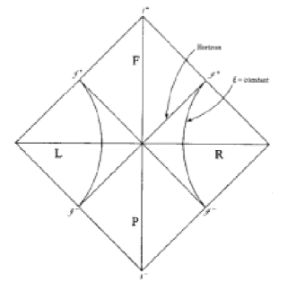
Given the two bases, we can perform the mode decomposition for a scalar field satisfying the trivial wave equation $\kern 0.5pt{\lower 0.1pt\vbox{\hrule height=0.5pt,width=6.8pt\hbox{\vrule width=0.5pt,height=6.0pt\kern 6.0pt\vrule width=0.3pt} \hrule height=0.3pt,width=6.8pt}}\kern 1.5pt\phi=0$. In Minkowski null coordinates $(\bar{u},\bar{v})$ one gets the standard orthonormal mode solutions

$$\bar{u}_{k} = \frac{1}{\sqrt{4\pi\omega}}e^{{\mathrm{i}}kx-{\mathrm{i}}\omega t}$$ (1.146)

$$\omega = |k|,\qquad-\infty<k<+\infty$$

These modes have positive frequency with respect to the standard global Killing vector of Minkowski $\partial_{t}$

$${\cal L}_{\partial_{t}}\bar{u}_{k}=-{\mathrm{i}}\omega\bar{u}_{k}$$ (1.147)

In the case of the Rindler observers, we shall have that the wave equation is unchanged thanks to its conformal invariance but we shall have to take into account that two sets of modes (one for the right wedge and one of the left wedge) are now necessary. Actually it is easy to see that the future-pointing timelike Killing vector field is $+\partial_{\eta}$ in the right wedge and $-\partial_{\eta}$ in the left wedge and so two different definitions of positive frequency will exist in the two wedges

$$R: {\cal L}_{+\partial_{\eta}}{}^{R}u_{k}=-{\mathrm{i}}\omega{}^{R}u_{k}\quad\mbox{and}\quad=0\quad\mbox{in the left wedge}$$ (1.148)

$$L: {\cal L}_{-\partial_{\eta}}{}^{L}u_{k}=-{\mathrm{i}}\omega{}^{L}u_{k}\quad\mbox{and}\quad=0\quad\mbox{in the right wedge}$$ (1.149)

where the superscripts $R$ and $L$ identify the right and left wedge modes respectively. So we shall have two bases each of which is complete in its respective wedge but not complete over the whole manifold

$${}^{R}u_{k} = \frac{1}{\sqrt{4\pi\omega}}e^{{\mathrm{i}}k\xi-{\mathrm{i}}\omega\eta}$$ (1.150)

$${}^{L}u_{k} = \frac{1}{\sqrt{4\pi\omega}}e^{{\mathrm{i}}k\xi+{\mathrm{i}}\omega\eta}$$ (1.151)

$$\omega = |k|,\qquad-\infty<k<+\infty$$

with ${}^{R}u_{k}=0$ in $L$ and ${}^{L}u_{k}=0$ in $R$.

At this point is easy to see that the field will admit two different mode decompositions

$$\phi = \sum_{k=-\infty}^{+\infty}{\left(a_{k}\bar{u}_{k}+a^{\dagger}\bar{u}^{*}_{k}\right)}$$ (1.152)

$$\phi = \sum_{k=-\infty}^{+\infty}{\left({}^{L}b_{k}{}^{L}u_{k}+{}^{L}b^{\dagger}_{k}{}^{L}u^{*}_{k}+{}^{R}b_{k}{}^{R}u_{k}+{}^{R}b^{\dagger}_{k}{}^{R}u^{*}_{k}\right)}$$ (1.153)

The Minkowski vacuum will then be defined as $a_{k}|0\rangle_{\mathrm{Mink}}\equiv 0$ and the Rindler vacuum will be defined as ${}^{L}b_{k}|0\rangle_{L}={}^{R}b_{k}|0\rangle_{R}\equiv 0$. These two vacua are clearly inequivalent due to the different mode structure but to actually see how many Rindler particles are present in the Minkowski vacuum one has to find the Bogoliubov transformations relating the two bases [4, 5]. The net result is that

$$\langle 0|{}^{(L,R)}b^{\dagger}_{k}{}^{(L,R)}b_{k}|0\rangle_{\mathrm{Mink}}=\frac{e^{-\pi\omega/a}}{[2\sinh(\pi\omega/a)]}=\frac{1}{e^{2\pi\omega/a}-1}$$ (1.154)

and so we see that the Minkowski vacuum appears to the Rindler observer as a thermal bath at a temperature $T=a/2\pi k_{\mathrm{B}}$.

Before continuing, some remarks are in order

• A general remark that should always be taken into account is that in order to state that “an observer sees a given vacuum as” one cannot generally rely just on the results from the Bogoliubov coefficients. As we said in section 1.1.2, the presence of typically quantum interference terms in the expression of the SET as a function of the Bogoliubov coefficients makes the above statement unsafe if just based on non-null $\beta$ coefficients. One should always base this sort of statement on more reliable tools such as analysis of particle detectors [4].

  Nevertheless in the special cases in which one gets a thermal nature for the emitted radiation, the quantum correlations are lost and the interference terms vanish. It is then possible to limit the analysis to the Bogoliubov transformations.

• It should be stressed that no real quanta are created. The total SET is covariant under coordinate transformation and so if it is equal to zero in Minkowski (as it is set by definition), it should be zero also for accelerated observers. In fact it can be shown that the expectation value of the SET in the (Rindler) vacuum state of the accelerated observer is non zero but corresponds to a vacuum polarization which is equivalent to subtracting from the Minkowski vacuum a thermal bath at the Unruh temperature [66, 67]. This contribution exactly cancels out the other one coming from the fact that a thermal bath of real particles is actually experienced from the Rindler observer. So in each wedge

  $$\langle 0|T_{\mu\nu}|0\rangle_{\mathrm{Mink}}=0=\langle 0|T_{\mu\nu}|0\rangle_{\mathrm{Rindler}}+\mbox{Thermal bath}$$ (1.155)

  Physically this tells us that we can regard the non-equivalence of the Minkowski and Rindler vacua as an example of vacuum polarization.

• The thermal distribution can be seen as an effect of the apparent horizon at $\bar{u}=\bar{v}=0$ experienced by the Rindler observer. This apparent horizon is similar to the event horizon of a black hole although it has a less objective reality: it is dependent on the state of motion of some observers and is not observed, for example, by Minkowski observers.

  Moreover this apparent horizon can be globally defined for observers who have undergone a uniform acceleration for an infinite time. In the case of uniform acceleration for a finite time, the thermal spectrum is replaced by a more complicated and general distribution.

Having developed a good understanding about the effects linked to the presence of Killing horizons in flat space, we can now move to the case of particle creation around black holes.

Hawking Radiation

In order to take full advantage of the above results we can concentrate on the case of a two-dimensional Schwarzschild black hole. The metric in this case is given by

$${\mathrm{d}}s^{2}=\left(1-\frac{2M}{r}\right){\mathrm{d}}t^{2}-\left(1-\frac{2M}{r}\right)^{-1}{\mathrm{d}}r^{2}$$ (1.156)

We can start by passing, as we did before, to the convenient null coordinates

$$\left.\begin{array}[]{lll}u&=&t-r-2M\ln\left|\frac{\textstyle r}{2M}-1\right|\\ &&\\ v&=&t+r+2M\ln\left|\frac{\textstyle r}{2M}-1\right|\end{array}\right\}$$

In these null coordinates the black hole metric takes the form

$${\mathrm{d}}s^{2}=\left(1-\frac{2M}{r}\right){\mathrm{d}}u{\mathrm{d}}v$$ (1.157)

Together with this null coordinate system, which is appropriate for static observers at infinity, we shall consider another set of coordinates, the so called Kruskal coordinates defined as

$$\left.\begin{array}[]{lll}\bar{u}&=&-\kappa^{-1}e^{-\kappa u}\\ \bar{v}&=&\kappa^{-1}e^{\kappa v}\end{array}\right\}$$ (1.158)

where $\kappa$ is the surface gravity of the black hole and in our specific case is $1/4M$. The Kruskal coordinates are appropriate for observers freely falling into the black hole (but still outside it) and we can see that the metric is perfectly well defined also on the event horizon in this system

$${\mathrm{d}}s^{2}=\left(\frac{2M}{r}\right)e^{-r/2M}{\mathrm{d}}\bar{u}{\mathrm{d}}\bar{v}$$ (1.159)

These coordinates allow us to build up the so called maximal analytic extension of the black hole spacetime to which can be associated the conformal diagram shown in figure 1.4.

Figure 1.4: Conformal diagram of Schwarzschild spacetime (picture reproduced from [4]).

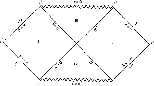
The regularity of the Kruskal coordinates also has an important consequence when we look at the two basis modes for the usual wave equation $\kern 0.5pt{\lower 0.1pt\vbox{\hrule height=0.5pt,width=6.8pt\hbox{\vrule width=0.5pt,height=6.0pt\kern 6.0pt\vrule width=0.3pt} \hrule height=0.3pt,width=6.8pt}}\kern 1.5pt\phi=0$. In fact these bases will be either proportional to $e^{-{\mathrm{i}}\omega u},e^{-{\mathrm{i}}\omega v}$ in the Schwarzschild observer’s system or to $e^{-{\mathrm{i}}\omega\bar{u}},e^{-{\mathrm{i}}\omega\bar{v}}$ in the Kruskal one. The regular behaviour of the Kruskal coordinates on the horizon then implies that while the first set above will oscillate infinitely rapidly near to the horizon, the second one will be regular over the whole manifold.

This different behaviour of the two mode bases is reminiscent of what we saw in the Rindler case where the Rindler system of coordinates is indeed badly defined at the (apparent) horizon and does not cover the whole of Minkowski spacetime. Actually if we now confront the form of the transformation above with those relating the null coordinates of the Minkowski and Rindler observers, equation (1.144), it is easy to see that there is a close relation between the Kruskal observers and the Minkowskian ones and between Schwarzschild and Rindler ones. In this case the role of the acceleration is played by the surface gravity of the black hole.

Also in this case we see that the introduction of two separate sets of Schwarzschild modes will be needed in order to expand the scalar field on the whole manifold. One set will cover the asymptotically flat zone I of the conformal diagram 1.4 the other covers the specular zone II.

So, in strict analogy with what we did in the Rindler case, we get the two mode expansion in Kruskal and Schwarzschild coordinates as

$$\phi = \sum_{k=-\infty}^{+\infty}{\left(a_{k}\bar{u}_{k}+a^{\dagger}\bar{u}^{*}_{k}\right)}$$ (1.160)

$$\phi = \sum_{k=-\infty}^{+\infty}{\left({}^{II}b_{k}{}^{II}u_{k}+{}^{II}b^{\dagger}_{k}{}^{II}u^{*}_{k}+{}^{I}b_{k}{}^{I}u_{k}+{}^{I}b^{\dagger}_{k}{}^{I}u^{*}_{k}\right)}$$ (1.161)

We shall now have two vacuum states $a_{k}|0\rangle_{\rm S}=0$ and ${}^{(I,II)}b_{k}|0\rangle_{\rm K}=0$ to relate via Bogoliubov transformations and we can again expect a thermal distribution

$$\langle 0|{}^{(I,II)}b^{\dagger}_{k}{}^{(I,II)}b_{k}|0\rangle_{\rm K}=\frac{e^{-\pi\omega/\kappa}}{[2\sinh(\pi\omega/\kappa)]}=\frac{1}{e^{2\pi\omega/\kappa}-1}$$ (1.162)

So we see that the Kruskal vacuum appears to the Schwarzschild observers at infinity as a thermal bath at temperature $T=\kappa/2\pi k_{\mathrm{B}}$.

It is interesting to see that the relation between the two vacua can be written in the form [4]

$$|0\rangle_{\rm K} = \exp\left\{{\textstyle\sum}_{k}\left[-\ln\cosh(\zeta_{\omega})+\tanh(\zeta_{\omega}){}^{I}b^{\dagger}_{k}{}^{II}b^{\dagger}_{k}\right]\right\}|0\rangle_{\rm S}$$ (1.163)

$$= {\textstyle\prod}_{k}\left(\cosh(\zeta_{\omega})\right)^{-1}{\textstyle\sum}^{\infty}_{n_{k}=0}e^{-n_{k}\pi\omega/\kappa}|{}^{I}n_{k}\rangle|{}^{II}n_{k}\rangle$$

where we have defined $\exp(-\pi\omega/\kappa)\equiv\tanh(\zeta_{\omega})$, and in the last line we have introduced states with ${}^{I}n_{k}$ particles in region I and ${}^{II}n_{k}$ particles in region II. We now see a behaviour which is in strict relation with what we said about squeezed states and thermality. In fact if we consider the measurement of an observable $\hat{A}$ by an observer “living” in region I we find that the states of region II will simply factor out

$$\langle 0|\hat{A}|0\rangle_{\rm K} = \sum_{n_{k}}\prod_{k}\langle{}^{I}n_{k}|\hat{A}|{}^{I}n_{k}\rangle\exp(-2n_{k}\pi\omega/\kappa)\times\left[1-\exp(-2\pi\omega/\kappa)\right]$$ (1.164)

$$= \mathrm{Tr}\left(\hat{A}\rho\right)$$

where, setting $E_{n}=n\omega$ and $\beta=2\pi/\kappa$, $\rho$ can be regarded as density matrix corresponding to a thermal average

$$\rho=\sum_{n}\prod_{k}\frac{e^{\beta E_{n}}}{\sum_{m=0}^{\infty}e^{-\beta E_{m}}}|{}^{II}n_{k}\rangle\langle{}^{II}n_{k}|$$ (1.165)

In the particular case where $\hat{A}$ is the particle number operator then we can easily see that from (1.164) we get the expected thermal distribution.

The emergence of thermality in black hole is again a particular case of the more general property of squeezed states. Nevertheless, as we said, the fact that for each pair of particles created from the vacuum, one gets lost for ever into the black hole is an indication that in this special case the distinction between the squeezed state and thermal one disappears.

Before ending this section and this chapter we should stress some important issues related to the Hawking effect.

• In the derivation sketched above, the modes that are associated with purely outgoing particles with respect to static observers at ${\cal I}^{+}$ are $\exp(-i\omega u)$. These can be traced back in time and appear as outgoing from ${\cal H}^{-}$ where the appropriate coordinates are those of Kruskal. Now the Kruskal transformations (1.158) imply that any time interval $\Delta u$ on ${\cal I}^{+}$ is stretched on ${\cal H}^{-}$, $\Delta\bar{u}=-\kappa^{-1}\exp(-\kappa\Delta u)$. Conversely the frequencies will get a blueshift factor $\exp(\kappa u)$ when one traces the modes back from ${\cal I}^{+}$ to ${\cal H}^{-}$. This in particular implies that the frequencies of the outgoing modes on ${\cal I}^{+}$ in proximity of the future event horizon ${\cal H}^{+}$ (that is for $u\to\infty$) are going to be infinitely blueshifted on ${\cal H}^{-}$. Actually before arriving at the horizon some modes will get frequencies larger than the Planck one $\omega_{pl}=2\pi/t_{pl}$ and so the semiclassical approximation should break down. Apparently Hawking radiation should be dominated by high frequency modes that would lead to a failure of the whole framework used to derive the effect. This is called the problem of transplanckian frequencies. We shall see in chapter 3 how such an unphysical feature can be interpreted and possibly circumvented.

• We have just seen a very easy example of the Hawking effect in two dimensions and for a conformally invariant wave equation. In four dimensions the calculations are much more difficult and in particular if we write the generic solution as

  $$\phi=\frac{R_{\omega l}(r)}{r}Y_{lm}(\theta,\varphi)e^{-{\mathrm{i}}\omega t}$$ (1.166)

  then from the radial part of the standard wave equation $\kern 0.5pt{\lower 0.1pt\vbox{\hrule height=0.5pt,width=6.8pt\hbox{\vrule width=0.5pt,height=6.0pt\kern 6.0pt\vrule width=0.3pt} \hrule height=0.3pt,width=6.8pt}}\kern 1.5pt\phi=0$ one gets

  $$\frac{{\mathrm{d}}^{2}R_{\omega l}}{{\mathrm{d}}{r^{*}}^{2}}+\left\{\omega^{2}-\left[l(l+1)r^{-2}+2Mr^{-3}\right]\left[1-2Mr^{-1}\right]\right\}R_{\omega l}=0$$ (1.167)

  where $r^{*}=r+2M\ln|(r/2M)-1|$ is the so called “tortoise” coordinate.

  Analytical solutions of these equations in terms of simple functions are not available. This has led to elaborate analytical approximations [68, 69, 70] as well to numerical techniques (see [71] and reference therein).

• The potential terms appearing in square brackets in Eq.(1.167) lead to backscattering of the incoming waves by the gravitational field. As a consequence of this the spectrum of particles reaching future infinity will not be purely thermal but will show an overall grey-body factor.

• The vacuum states $|0\rangle_{\rm S}$ and $|0\rangle_{\rm K}$ are not the only ones which can be defined on the eternal black hole manifold. Different initial conditions on the incoming/outgoing modes will generically correspond to different vacuum states. This subtle issue is not important for the remaining discussion in this thesis and we refer the reader to fundamental papers on the subject (see e.g. [67]) and standard textbooks [4, 5, 8].

• We have considered the case of an eternal black hole but also the more realistic case of particle creation from gravitational collapse can be studied [4, 5, 8]. We shall consider in the next chapter an example of gravitational collapse which will apply the standard technique for computing particle production. It should be stressed that the aforementioned ambiguity about the construction of vacuum states in the eternal case is absent in the case of collapsing bodies.

With these remarks on the Hawking effect we close this introductory chapter concerning the effects of the quantum vacuum in strong fields. We have seen that the new role that vacuum has in modern physics automatically leads to the prediction of interesting effects such as polarization and particle production from the vacuum. Although we have experimental tests of the static Casimir effect we still lack any test of particle production from nonstationary external fields, the phenomenon which in the case of gravity takes the name of Hawking radiation.

The next step in our investigation will now be the discussion of the consequences of the results described above. In particular we shall concentrate our attention on black hole thermodynamics because of its role as a bridge towards quantum gravity and we shall need to make full use of all of the concepts learned so far.

Chapter 2 Quantum Black Holes

As far as the laws of mathematics refer to reality

they are not certain;

and as far as they are certain,

they do not refer to reality.

Albert Einstein

In this chapter we shall deal with the quantum aspects of black hole physics, that is with the most famous application of the theory of the quantum vacuum in gravitational fields. We shall review the basic notions of this fascinating field of research and discuss its importance as the key to disclosing the basic properties that a quantum theory of gravity should have. We shall focus our attention on the interpretation of black hole entropy and study its relation with the global structure of spacetime. From this study we shall move towards an interpretative proposal for black hole thermodynamics based on the zero point modes of the quantum fields. The aim of such a proposal is to unify the Casimir effect and the early Sakharov idea of induced gravity. We shall finally discuss in detail the special role that extremal solutions have. The formation of extremal black holes from gravitational collapse will then be studied to give us further insight into this issue. At the end of the chapter we shall present some speculations about the framework emerging from the research in this field.

2.1 Black Hole Thermodynamics

Although Hawking’s discovery of quantum radiation from black holes in 1975 [72] was completely unexpected by most of the experts of that time, it should be stressed that the new paradigm, of a thermodynamical behaviour of black holes, was already starting to emerge a few years before.

The first understanding that classical black hole physics was outrageously in conflict with our basic thermodynamical notions is generally ascribed to Wheeler. In particular a black hole, by engulfing an object endowed with a given entropy $\sigma$, would be able to reduce the total entropy of the universe and in this way would lead to a violation of the second law of thermodynamics.

This sort of observation led Bekenstein [73, 74] to postulate that a black hole should be endowed with a proper entropy. Given the fact that the area of a black hole never decreases in a classical process [75, 76] then he could argue that this quantity plays a role similar to entropy.

From this starting consideration the research on black hole physics achieved a series of theoretical results that brought an elegant and impressive formulation of some General Relativity theorems as thermodynamical laws. The full awareness of the existence of a sort of “black hole thermodynamics” then found its systematic statement in a seminal paper by Bardeen, Carter and Hawking [77].

What was found was that for each classical thermodynamical law it is possible to formulate a corresponding one for black holes. These results are collected in the table below.

Law	Thermodynamics	Black Holes
Zeroth	T is constant throughout	The surface gravity $\kappa$ is
	bodies at thermal equilibrium	constant on the event horizon
		of a stationary black hole
First	${\mathrm{d}}E=T{\mathrm{d}}s+\mbox{work terms}$	The mass of a black hole
		is related to its area $A$,
		surface gravity $\kappa$ and
		angular momentum $J$ by
		the equation ${\mathrm{d}}M={{\kappa}\over{2\pi}}{\mathrm{d}}A+\Omega{\mathrm{d}}J$
		where $\Omega$ is the angular velocity of the black hole
Second	$\delta S\geq 0$ in any process	$\delta A\geq 0$ in any processes
		satisfying the WEC
Third	It is impossible to achieve	It is impossible to achieve
	the $T=0$ state by a	the $\kappa=0$ state
	physical process in a	(aka extremal state)
	finite number of steps	by a physical process in a
		finite number of steps

Although these results were very impressive, the new paradigm became fully consistent only with the discovery of Hawking radiation by the application of quantum field theory in curved space. In fact it is impossible to define a temperature for classical black holes, thus it is strictly not even reasonable to talk about entropy in this case. As discussed before, Hawking proved that, due to the polarization of the vacuum in the vicinity of the black hole horizon, there is a thermal flux of radiation flowing out towards infinity. By the first law and the Hawking temperature

$$T_{\rm H}=\frac{\hbar\kappa}{2\pi ck_{\rm B}}$$ (2.1)

one finds the entropy of a black hole to be one quarter of its area [72]

$$S_{{\mathrm{BH}}}=\frac{Ak_{\mathrm{B}}}{4L_{\rm Pl}^{2}}$$ (2.2)

This quantity is the so-called Bekenstein–Hawking entropy. Sometimes it also takes the name of gravitational entropy and we shall use both terminologies in the rest of this work.

At this point it is perhaps worthwhile to say something more about the different status of the above quoted thermodynamical laws. In fact these do not share the same status or the same robustness.

• The zeroth law is a firm theorem of classical general relativity (which assumes the validity of the DEC to constrain the matter behaviour).

• The first law is also a general statement of energy conservation when a system incorporating a black hole switches from one stationary state to another, it can be rigorously proved at least for all the non-extremal black hole systems.

• The second law, in its classical formulation, follows from the so-called Hawking area theorem [75, 76]. As noted previously, this is a theorem of General Relativity which assumes the WEC. Notably the discovery of quantum radiation from black holes led also to a revision of the classical statement of the second law. In fact, if a black hole can evaporate due to Hawking radiation, then it is possible to reduce its mass and hence its area, i.e. its entropy. The point is that WEC is explicitly violated by Hawking radiation (and in general by all processes of quantum particle creation from vacuum).

  Already before Hawking’s discovery, Bekenstein [73, 78, 79] proposed that the generalized entropy, defined as the sum of the entropy of the black hole and that of radiation and matter outside the horizon,

  $$\tilde{S}=S_{{\mathrm{BH}}}+S_{{\mathrm{matter}}}$$

  is an always increasing quantity

  $$\Delta\tilde{S}=\Delta S_{{\mathrm{BH}}}+\Delta S_{{\mathrm{matter}}}\geq 0$$

  Later, analytical as well numerical results [80, 81] corroborated this analogy which is now generally stated as the generalized second law. No counter-examples, able to violate this general formulation of the second law, have so far been found. Nevertheless it is important to stress the intrinsically conjectural nature of the above relation and its intrinsic assumption of the similar nature of gravitational entropy and quantum matter entropy.

• The third law stands on a much less firm basis than the other ones. First of all it is important to stress that even the standard third law of thermodynamics admits at least two different formulations both due to Nernst.

  The first statement of the third law, aka the Nernst law, states that the zero temperature states of a system are isentropic. If $\Delta S$ is the difference between the entropies of two states of a thermodynamical system then $\lim_{T\rightarrow 0^{+}}\Delta S=0$. This implies that the entropy of all of the states at absolute zero temperature does not depend on any other macroscopic parameter, it is a constant. Planck’s postulate assumes that this constant is strictly zero.

  The second statement, aka the Unattainability law, states the impossibility of reaching the absolute zero temperature by a finite number of thermodynamical processes.

  Although it is generally true that the above two formulations of the third law are equivalent, this is not always true as stated even in some textbooks of thermodynamics [82]. The black hole case is, in this sense, a typical example where the Nernst formulation is violated but the unattainability one holds (this was first recognized by Davies in [83]). In fact the third law as stated above is exactly a formulation, for black holes, of the unattainability law. Although in [77] this had just the form of an analogy it was later on reformulated and rigorously proved by Israel [84]. Nowadays the general statement is: A non-extremal black hole cannot become extremal at a finite advanced time in any continuous process in which the stress-energy tensor of accelerated matter stays bounded and satisfies the WEC in the neighborhood of the outer apparent horizon.

  The fact that the Nernst formulation does not follow from the Unattainability one is also a major cause for being extremely suspicious about some common statements, in the existing literature, on the failure of the Planck postulate in black hole thermodynamics. In fact it is generally stated that since the area of extremal black holes is not zero then the entropy as well cannot be zero. This simple deduction assumes that the Bekenstein–Hawking formula holds also in the extremal limit. This would be safe if a) there are no multiple branches in the thermodynamic configuration space, b) there is no discontinuity in thermodynamic properties of the system near to absolute zero. Both of these assumptions can in principle be violated if the Unattainability formulation does not imply the Nernst one. This kind of analysis has been carried out for black hole thermodynamics in [85]. We shall indeed see, later on in this chapter, how semiclassical calculations seem to actually suggest the break down of the area law in the extremal limit.

As a final remark it should be said that although the laws of black hole thermodynamics are actually derived as theorems of General Relativity (and so are substantially encoded at a classical level), the notion of temperature for a black hole emerges just as a quantum effect on the curved background. How could General Relativity “be aware” of the role of quantum fields? How deep is the relation between the Hawking radiation and the thermodynamical properties of black holes? It should be stressed that this appears nowadays as one of the the key points for the whole understanding of the subject.

We shall see later that concepts like gravitational entropy and Hawking radiation are not necessarily linked and that the Bekenstein-Hawing formula appears as a general behaviour that emerges in a whole class of theories of gravitation and is largely independent of whatever quantum theory of gravity is assumed. Apart from this issue other ones arose rapidly after Hawking’s discovery and are still now the subject of investigation. We cannot present all of these here, so we shall limit our discussion to the two other fundamental points that have polarized research in this field in the last twenty years.

The first of these issues deals with the role of Hawking radiation in the final destiny of black holes and is often quoted as the puzzle of Information loss. Information loss is related to the fact that black hole evaporation by means of emission of a thermal particle spectrum, appears to produce a destruction of quantum information by converting a pure state into a mixed one. Hawking suggested that this should be a starting point for a generalization of quantum mechanics in which non-unitary evolution of quantum states in the presence of strong gravitational fields is allowed [86, 87].

In disagreement with Hawking’s point of view, several attempts have been made in order to circumvent this apparent break down of standard quantum mechanics. We shall limit ourselves here to a brief sketch of the different proposals (see [8, 88] for a comprehensive review)

• Information is released via Hawking radiation. Although this may appear as a natural solution, it implies the discovery of some mechanism by which the information hidden inside the black hole can be fully “encoded” on the horizon and then taken away by the radiation.

• Information is released at the end of evaporation. The idea of a final “burst of information” assumes that a large amount of energy is still available at the end of the evaporation in order to allow a huge transmission of information. Unfortunately it appears very difficult to sustain this assumption.

• The information is simply “stored” in a remnant which is the final outcome of the black hole evaporation. In this framework the information of an arbitrarily massive black hole should always be storable in a Planck-size object which, in order to do so, should be endowed with an extremely large number of internal states.

• The information escapes to “baby universes”. The black hole formation does not lead to the presence of a singularity inside the horizon. The collapsing body will instead form a closed baby universe to which the information is passed.

• Quantum Hair. The no hair theorem is not true at a quantum level and some black hole hair can give partial information about the matter that has formed the black hole.

The second issue is related to the statistical origin of the gravitational entropy and this will be the subject of the next section.

2.2 Alternative derivations of the black hole entropy

After the initial discovery of black hole thermodynamics, other techniques were developed and found capable of obtaining the same results from rather different approaches. We shall briefly discuss these alternative formulations of black hole thermodynamics.

2.2.1 Euclidean derivation of black hole Thermodynamics

Semiclassical Euclidean quantum gravity techniques play a key role in the investigation of the thermodynamics of black holes. We shall here summarize the path integral approach procedure following the steps first delineated by Gibbons and Hawking [89].

Given the classical Einstein–Hilbert action for gravity and the action of classical matter fields, one formulates the Euclidean path integral by means of a Wick rotation $t\rightarrow-{\mathrm{i}}\tau$ .

In particular if one considers the Einstein–Hilbert action plus a matter contribution in the generating functional of the Euclidean theory, one finds that the dominant contribution to the Euclidean path integral is given by gravitational instantons (i.e. non-singular solutions of the Euclidean Einstein equations).

In spacetimes with event horizons, metrics extremizing the Euclidean action are gravitational instantons only after removal of the conical singularity at the horizon [89]. A period must therefore be fixed in the imaginary time, $\tau\rightarrow\tau+\beta$, which becomes a sort of angular coordinate.

To be concrete we can take the standard Schwarzschild metric in Euclidean signature:

$${\mathrm{d}}s^{2}_{\mathrm{E}}=\left(1-\frac{r_{\mathrm{h}}}{r}\right){\mathrm{d}}\tau^{2}+\left(1-\frac{r_{\mathrm{h}}}{r}\right)^{-1}{\mathrm{d}}r^{2}+r^{2}{\mathrm{d}}\Omega^{2}$$ (2.3)

This solution still shows singularities at $r=r_{\mathrm{h}}=2M$ and $r=0$. If we now define a new radial variable, $\rho=2\sqrt{r-r_{\mathrm{h}}}$, the metric acquires the form

$${\mathrm{d}}s^{2}_{\mathrm{E}}=\left(\frac{\rho^{2}}{4}+r_{\mathrm{h}}\right)^{-1}\frac{\rho^{2}}{4}{\mathrm{d}}{\tau}^{2}+\left(\frac{\rho^{2}}{4}+r_{\mathrm{h}}\right){\mathrm{d}}\rho^{2}+\left(\frac{\rho^{2}}{4}+r_{\mathrm{h}}\right){\mathrm{d}}\Omega^{2}$$ (2.4)

For $\rho\rightarrow 0$ one then gets:

$${\mathrm{d}}s^{2}_{\mathrm{E}}=\frac{1}{r_{\mathrm{h}}}\frac{\rho^{2}}{4}{\mathrm{d}}{\tau}^{2}+r_{\mathrm{h}}{\mathrm{d}}\rho^{2}+r_{\mathrm{h}}^{2}{\mathrm{d}}\Omega^{2}$$ (2.5)

If one now defines $\bar{\rho}\equiv\rho\sqrt{r_{\mathrm{h}}}$ and $\bar{\tau}\equiv\tau/(2r_{\mathrm{h}})$ the metric takes the so called conical form:

$${\mathrm{d}}s^{2}_{\mathrm{E}}=\bar{\rho}^{2}{\mathrm{d}}{\bar{\tau}}^{2}+{\mathrm{d}}\bar{\rho}^{2}+r_{\mathrm{h}}^{2}{\mathrm{d}}\Omega^{2}$$ (2.6)

Smoothness at $\bar{\rho}=0$ requires the previously mentioned periodicity in the imaginary time. The required period $\beta$ corresponds exactly to the inverse Hawking–Unruh temperature $\beta_{\mathrm{H}}=2\pi/\kappa$ because of the relation between the periodicity of the Euclidean Green’s functions and the thermal character of the corresponding Green’s functions in Lorentzian signature. Hence, in these cases, the effective action is truly a free energy function $\beta F$. In such a way thermodynamics appears as a requirement of consistency of quantum field theory on spacetimes with Killing horizons, and in this sense we shall define such a thermodynamics as “intrinsic”.

It is important to stress that the situation changes dramatically in the case of extremal black holes. In fact the general form of the metric is now

$${\mathrm{d}}s^{2}_{\mathrm{E}}=\left(1-\frac{r_{\mathrm{h}}}{r}\right)^{2}{\mathrm{d}}\tau^{2}+\left(1-\frac{r_{\mathrm{h}}}{r}\right)^{-2}{\mathrm{d}}r^{2}+r^{2}{\mathrm{d}}\Omega^{2}$$ (2.7)

Performing the same transformations as before this can be cast in the form:

$${\mathrm{d}}s^{2}_{\mathrm{E}}=\left(\frac{\rho^{2}}{4}+r_{\mathrm{h}}\right)^{-2}\left(\frac{\rho^{2}}{4}\right)^{2}{\mathrm{d}}{\tau}^{2}+\left(\frac{\rho^{2}}{4}+r_{\mathrm{h}}\right)^{2}\frac{4}{\rho^{2}}{\mathrm{d}}\rho^{2}+\left(\frac{\rho^{2}}{4}+r_{\mathrm{h}}\right){\mathrm{d}}\Omega^{2}$$ (2.8)

which in the $\rho\rightarrow 0$ limit gives

$${\mathrm{d}}s^{2}_{\mathrm{E}}=\left(\frac{1}{r_{\mathrm{h}}}\right)^{2}\frac{\rho^{4}}{16}{\mathrm{d}}{\tau}^{2}+\frac{4r^{2}_{h}}{\rho^{2}}{\mathrm{d}}\rho^{2}+r_{\mathrm{h}}^{2}{\mathrm{d}}\Omega^{2}$$ (2.9)

It is now easy to see that in this case passing to a system of coordinates equivalent to the previous one given by $\bar{\tau}$ and $\bar{\rho}$ does not give rise to any “conical-like” metric. This implies that, for extremal black holes, there is no way to fix the period of the imaginary time and hence the intrinsic temperature. We shall see later on, in section 2.4, how these considerations are strictly related with the emergence of a gravitational entropy in spacetimes with event horizons.

Coming back to the issue of the Euclidean formulation of black hole thermodynamics we can now consider the partition function for solutions where a temperature can be fixed in the way described above.

The partition function in a canonical ensemble $Z$ can be written in the case that one includes also the gravitational field

$$Z={\rm{Tr}}\;\exp{[-(\beta{\cal H})]}=\int{\cal D}\left[\phi,g_{\mu\nu}\right]\exp{\left[-I\left(\phi,g_{\mu\nu}\right)\right]},$$ (2.10)

Using the fact that a black hole solution is an extremum of the (Euclidean) gravitational action, at the tree level of the semiclassical expansion one then obtains

$$Z\sim\exp{[-I_{\rm E}]}\,,\qquad I_{\rm E}={{1}\over{16\pi}}\int_{M}\left[\left(-R+2\Lambda)+L_{{\mathrm{m}}}\right)\right]+{{1}\over{8\pi}}\int_{\partial{M}}\left[K\right],$$ (2.11)

where $I_{\rm E}$ is the on-shell Euclidean action and $[K]=K-K_{0}$ is the difference between the extrinsic curvature of the manifold and that of a reference background. The Euclidean action is related to the free energy $F$ as $I_{\rm E}=\beta_{\mathrm{H}}F$ and the corresponding entropy is

$$S\equiv\beta^{2}\frac{\partial F}{\partial\beta}$$ (2.12)

Comment: It has to be stressed here that the procedure just presented has some subtleties that are well studied in the literature. One of these is that the Schwarzschild solution is a saddle point of the Euclidean effective action corresponding to an unstable solution. This is related to the fact that any black hole in vacuum is a thermally unstable object (as can be seen by the negative value of its heat capacity $C_{{\mathrm{BH}}}=-8\pi M^{2}$); but of course any self-gravitating system shows such a behavior, due to the attractive nature of gravity. The problem of performing a thermodynamical analysis of black holes, considering a grand-canonical ensemble, has been studied thoroughly by York [90], who suggested considering a black hole in a box. Such a choice automatically stabilizes the black hole and enables one to perform further semiclassical calculations. One can also consider the higher-order corrections to the action. Unfortunately neither one-loop graviton contributions [91] nor matter ones [9] seem to be able to stabilize the black hole, since they are small in comparison with the tree-level term, at least in the regime of negligible back reaction.

An interesting feature of the Euclidean path integral approach, is to show a link between the thermal properties of the black hole spacetimes and their global, topological structure. This has led Hawking and collaborators [92, 93] to suggest that black hole entropy has a topological origin. We shall come back to this issue later on in section 2.4.

2.2.2 Derivation of black hole entropy as a Noether Charge

Among alternative derivations of black hole thermodynamics, the so called Noether charge approach has attracted growing attention because of the central role that it appears to give to the symmetry under diffeomorphisms and the “localization” of the black hole entropy on the event horizon. Both of these features have become part of modern interpretations of black hole thermodynamics as we shall see in the next section.

Wald and collaborators [94, 95] demonstrated that the first law of black hole thermodynamics can be reformulated in any diffeomorphism-invariant theory in the presence of bifurcate Killing horizons . From this reformulation one gets that the gravitational entropy can be identified with the Noether charge associated with the diffeomorphism invariance of the theory [94, 95].

The basic scheme for the derivation of the first law can be summarized in a few steps. Let us start with a Lagrangian density ${\cal L}(x,\phi,\phi_{,\alpha},\phi_{,\alpha\beta},...)$ invariant under diffeomorphism transformations $x^{\mu}\rightarrow x^{\mu}+\xi^{\mu}(x)$. Here $\phi$ is a complete set of dynamical variables (metric included).

The Noether current density associated with this symmetry of the theory, say ${\cal J}^{\alpha}(\phi,\xi)$ is by definition conserved. This implies that it can be written as:

$${\cal J}^{\alpha}(\phi,\xi)={{\cal N}^{\alpha\beta}}_{,\beta}\qquad{\cal N}^{\alpha\beta}={\cal N}^{[\alpha\beta]}$$ (2.13)

When the metric is a dynamical variable it is convenient to work with ordinary scalars and tensors instead of densities:

$$L=(-g)^{-1/2}{\cal L}\;\;\;J^{\alpha}=(-g)^{-1/2}{\cal J}^{\alpha}\;\;\;N^{\alpha\beta}=(-g)^{-1/2}{\cal N}^{\alpha\beta}$$ (2.14)

In this notation Eq.(2.13) takes the form

$$J^{\alpha}=N^{\alpha\beta}_{;\beta}$$ (2.15)

The integral of $N^{\alpha\beta}$ over a closed two-dimensional surface $\sigma$ is called the Noether charge of $\sigma$ relative to $\xi^{\alpha}$. It is a local function of the dynamical fields and is linear in $\xi^{\alpha}$ and in its derivatives.

$$N(\sigma,\xi)=\int_{\sigma}N^{\alpha\beta}{\mathrm{d}}\sigma_{\alpha\beta}$$ (2.16)

We now consider a stationary, axisymmetric, asymptotically flat spacetime with a bifurcate Killing horizon generated by the Killing vector $\chi^{\alpha}=\xi^{\alpha}_{(t)}+\Omega^{\mathrm{h}}\xi_{(\phi)}^{\alpha}$. We can reproduce all of the above steps in the case in which $\xi^{\alpha}=\chi^{\alpha}$ and $\Sigma$ is chosen to be the three-hypersurface that extends from asymptotic infinity up to the bifurcation surface.

Considering the variation of the Noether charge at the horizon resulting from the variation of the fields $\delta\phi$ from the background solution (keeping fixed $\chi^{\alpha}$), one finds that it is equal to the difference between the variations of the mass and the angular momentum of the system measured at infinity in a way which strictly resembles the first law:

$$\delta N(\sigma_{\mathrm{h}},\chi)=\delta M-\Omega^{\mathrm{h}}\delta J$$ (2.17)

Actually it is not difficult to show that, for black holes which are vacuum solutions of the Einstein equations, the above formula is exactly the first law of black hole thermodynamics which we saw before [95]. In fact for General Relativity one has

$$L = \frac{1}{8\pi}R$$

$$J^{\alpha} = \frac{1}{8\pi}\left[\chi^{[\alpha;\beta]}_{;\beta}+G^{\alpha}_{\beta}\chi^{\beta}\right]$$ (2.18)

where $G_{\alpha\beta}$ is the Einstein tensor. For vacuum solutions this tensor vanishes and then, using Eq.(2.15) it easy to recognize that

$$N^{\alpha\beta}=\frac{1}{8\pi}\chi^{[\alpha;\beta]}$$ (2.19)

Moreover from the fact that $\chi^{\alpha}$ is the generator of the event horizon it follows that:

$$N(\sigma_{\mathrm{h}},\chi)=\frac{1}{8\pi}\int_{\sigma}{\mathrm{d}}\sigma_{\alpha\beta}\chi^{[\alpha;\beta]}=\frac{1}{8\pi}\kappa A$$ (2.20)

So equation (2.17) takes exactly the standard form of the first law with $S=A/4$.

The most remarkable fact is that this relation is valid for any covariant theory and can then be interpreted as a generalization of the Einsteinian formula. If a diffeomorphism invariant theory does not contain higher than second order derivatives of the dynamical variables, the Noether charge $N(\sigma,\chi)$ can always be reduced to a linear function of $\chi^{\alpha}$ and its first derivative. Since the Killing vector is, by definition, null on the bifurcation surface, $\chi^{\alpha}=0$, then $N^{\alpha\beta}\sim\chi^{\alpha\beta}$.

Finally to obtain a value of the Noether charge independent of the normalization of the Killing vector one can simply divide $N(\sigma,\chi)$ by the surface gravity $\kappa$. The normalized quantity ${\tilde{N}}(\sigma,\chi)$ is then a purely local quantity dependent on the geometry and on the dynamical fields at the horizon. Using it in the analogue of the first law leads to a natural generalization of the gravitational entropy

$$S=\frac{2\pi}{\kappa}N(\sigma,\chi)=\frac{2\pi}{\kappa}\int_{\sigma}N^{\alpha\beta}{\mathrm{d}}\sigma_{\alpha\beta}$$ (2.21)

To conclude we just stress that the Noether charge approach has several advantages:

• The strict locality and the geometrical nature of the normalized Noether charge make it insensitive to any ambiguity in the definition of the Lagrangian (for example to the addition of a total divergence).

• The method does not require any “Euclideanization”, a step which is still not fully understood in QFT in curved spaces (see [96] for a discussion of the link between Euclidean methods and Noether charge approach).

• Although the original Wald derivation relied on the presence of a bifurcation surface, nevertheless the entropy can be calculated by performing the integral over any arbitrary slice of the horizon of a stationary black hole [97].

To conclude the section we call attention to a crucial fact which is evident in this derivation of the gravitational entropy. It is notable that the black hole entropy can be so intimately related to the symmetry under diffeomorphisms of the theory, and that such a clean geometrical local nature (localized exactly on the event horizon) can be attached to it. Is there a deep link between symmetries and gravitational entropy? Is the Noether charge approach suggesting a localization on the horizon of the entropy? We shall discuss these issues again in the following section where we shall give a panoramic view of proposals advanced for explaining the origin of gravitational entropy.

2.3 Explanations of Black Hole entropy

As often in the history of science, the discovery of such a complex structure such as black hole thermodynamics opened a whole set of new questions to which complete answers are still lacking.

The problem of finding a dynamical origin for black hole entropy is the effort to achieve a statistical mechanics explanation of it. This means giving an interpretation of horizon thermodynamics in a “familiar” way, in the sense that it could be seen as related to dynamical degrees of freedom associated with black hole structure.

It is interesting to note that the terminology “black hole structure”, used above, is necessarily imprecise given the fact that there is still quite a heated debate in the literature about the location of these supposed degrees of freedom giving rise to the gravitational entropy. The enumeration of all of the proposals for explaining black hole entropy is out of the scope of this thesis. In what follows we shall try to present the main present tendencies. In order to make such a classification easier to follow we shall accumulate different proposals, grouping them in three general classes.

2.3.1 Information based Approaches

The first class of explanations, at least in time, for the black hole entropy is that based on the “sum over possibilities”. The basic idea is that when a black hole forms we retain just minimal information about the initial state (for example the star) which produced it. The information about the collapsed matter is “cut off” by a strong gravitational field and the black hole “forgets” everything about its initial state except for the charges associated with long range forces: mass $M$, electrical charge $Q$ and angular momentum $J$ . This is the so-called No Hair Theorem [98]. In close analogy with standard thermodynamics it is then possible to associate an entropy with the black hole by counting all of the possible microscopic configurations of the initial system which would lead to the same black hole (that is to the same values of the macroscopic parameters $M,Q,J$). In this case the informational entropy (aka von Neumann entropy) would be

$$S_{I}=-\sum_{n}p_{n}\ln p_{n}$$ (2.22)

where $p_{n}$ are the probabilities of different initial states.

This general framework includes the early works of Bekenstein [79] and of Zurek and Thorne [99]. In this proposal the black hole entropy is related to the “logarithm of the number of quantum-mechanically distinct ways that the hole could have been made”. In this sense one should also note the proposal by York [100] who tried to identify the dynamical degrees of freedom at the origin of black hole entropy with the quasi-normal modes excited by the quantum evaporation process. Since the logarithm of the number of thermally excited modes at a given time is much less than $M^{2}$ (in the Schwarzschild solution $S=A/4=4\pi M^{2}$) York proposed to define the entropy as the logarithm of the number of distinct excitation states of these modes in the process of black hole evaporation. More recently Bekenstein and Mukhanov [101] proposed a slightly different way to explain the gravitational entropy in the context of a model where the mass (and hence the area) of the black hole is assumed to be quantized. In this sense one considers the black hole in a similar way to an atomic system, where the absorption/emission of quanta would correspond to the transition from some energy level to another. The entropy can then be related to the degeneracy $g(n)$ of the level $n$ in which the black hole is at a given moment: $S=\ln g(n)$. We stress the difference between this approach and the Zurek–Thorne one. While in the latter, the different initial states of matter (which could have led to the final black hole) are counted, in the Bekenstein–Mukhanov approach one counts different trajectories in the space of black hole parameters.

2.3.2 Quantum Vacuum Based Approaches

The gravitational field of a black hole induces strong changes in the structure of the quantum vacuum surrounding it. As discussed in the Introduction, even in flat space the vacuum can be seen as a physical medium characterized by the zero-point fluctuations of the physical fields. For eternal black holes the vacuum appears to be polarized by the black hole in such a way as to form a thermal atmosphere. It is then tempting to relate the modification in the vacuum structure around the black hole with the vacuum fluctuations around it.

In this direction there was an early paper by Gerlach [102] where the black hole entropy was related to the logarithm of the total number of vacuum fluctuation modes responsible for the emission of the black body radiation. Later, ‘t Hooft [103] proposed a toy model, aka the “brick wall model”, in which it was assumed that field modes vanish, encountering an effective boundary, on the Planck length scale from the event horizon. It is then possible to consider the thermodynamics associated with the fields restricted to the exterior of this boundary. The idea of ‘t Hooft was to identify the black hole entropy with those of the fields left outside the horizon/boundary in thermal equilibrium at the Hawking temperature. An easy calculation yields the formula:

$$S\sim\alpha\frac{A}{\lambda^{2}}$$ (2.23)

where $A$ is the surface area of the black hole, $\lambda$ is the proper distance of the “brick wall” from the horizon. For $\lambda\sim L_{\mathrm{Pl}}$ the above entropy is of the same order of magnitude as that of Bekenstein–Hawking.

A development of this model was subsequently proposed by Srednicki [104], Bombelli, Koul, Lee, Sorkin [105], Frolov, Novikov [106] and other works. The black hole entropy would be generated by dynamical degrees of freedom, excited at a certain time, associated with the matter in the black hole interior near to the horizon through non-causal correlation (EPR) with external matter. The ignorance of an observer outside the black hole about the modes inside the horizon is associated with a so-called entanglement entropy which is identified with the Bekenstein–Hawking one.

Entanglement Entropy

Let us consider a global Hilbert space ${\mathbf{H}}$ composed of two uncorrelated ones ${\mathbf{H}}_{1}$, ${\mathbf{H}}_{2}$.

$${\mathbf{H}}={\mathbf{H}}_{1}\otimes{\mathbf{H}}_{2}$$ (2.24)

A general state on ${\mathbf{H}}$ can be described as a linear superposition of states on the two Hilbert spaces

$$|\psi\rangle=\sum_{a,b}\psi(a,b)|a\rangle|b\rangle$$ (2.25)

One can define a global density matrix

$$\rho(a,a^{\prime},b,b^{\prime})=\psi(a,b)\psi^{*}(a^{\prime},b^{\prime})$$ (2.26)

The reduced density matrix for the subsystem $a$ is given by

$$\rho(a,a^{\prime})=\sum_{b=b^{\prime}}\psi(a,b)\psi^{*}(a^{\prime},b^{\prime})$$ (2.27)

Note that even if the general state (2.25) defined on the global Hilbert space is a pure one, the form of the reduced density matrix (2.27) shows that the corresponding state defined only in one subspace is a mixed one. This corresponds to an information loss that can be properly described by von Neumann entropy (which is zero for a pure state)

$$S_{1}=-\mathrm{Tr}(\rho_{a}\ln\rho_{a})$$ (2.28)

Let us now discuss the same issue in the black hole case. We can consider a stationary black hole and define ${\hat{\rho}\,}^{{\mathrm{total}}}$, the density matrix describing, in Heisenberg representation, the initial state of quantum matter propagating on its background. For an external observer the system consists of two parts: the black hole and the radiation outside it. By defining a spacelike hypersurface we can consider quantum modes of radiation at a given time so that they can be separated into external ones and ones internal to the black hole.

The state for external radiation is obtainable from ${\hat{\rho}\,}^{{\mathrm{total}}}$ by tracing on all of the states of matter inside the event horizon and so inaccessible to the external observer

$${\hat{\rho}\,}^{{\mathrm{rad}}}=\mathrm{Tr}^{{\mathrm{inside}}}{\hat{\rho}\,}^{{\mathrm{total}}}$$ (2.29)

For an isolated black hole alone this density matrix would describe its Hawking radiation at infinity. We can also define the density matrix for the black hole state

$${\hat{\rho}\,}^{{\mathrm{BH}}}=\mathrm{Tr}^{{\mathrm{outside}}}{\hat{\rho}}^{{\mathrm{total}}}$$ (2.30)

where one now performs the trace on the external degrees of freedom. From this matrix it is possible to find the related von Neumann entropy

$$S^{{\mathrm{BH}}}=-\mathrm{Tr}^{{\mathrm{inside}}}(\hat{\rho}^{{\mathrm{BH}}}\ln\hat{\rho}^{{\mathrm{BH}}})$$ (2.31)

This is exactly what is called “entanglement entropy”. It is important to note that this definition is invariant in the sense that independent changes of definitions of the vacuum for the “external” and “internal” states do not change the value of $S^{{\mathrm{BH}}}$ [9].

Calculations of entanglement entropy were performed by various authors in a wide range of situations, in flat spaces as well as in curved ones. There are three common points that appear as proper characteristics of entanglement entropy:

1. Entanglement entropy is not a never-decreasing quantity. If the internal region is reduced by shrinking the division surface, the entanglement entropy goes to zero in the limit that all of the spacetime is again available to the external observer.

2. Entanglement entropy is always proportional to the area of the “division surface” (the event horizon in the black hole case).

3. Entanglement entropy is always divergent on the division surface due to the presence of modes of arbitrarily high frequency near to the horizon. The divergence form is general and independent of the kind of field.

The first point is a deep problem, casting some shadows on what the computation of entanglement entropy is effectively probing about black hole physics. Actually only in the Thermofield Dynamics framework which we introduced in section 1.3.3, does it appear possible to safely identify the entanglement entropy with the black hole one [58, 60].

Although the second point was initially one of the motivations for the identification of entanglement entropy with the Bekenstein–Hawking one, it was soon realized that such a behaviour is too general and appears to be valid even in flat space [104]. It is commonly felt that the special form of the Einstein equation and diffeomorphism invariance is at the root of black hole thermodynamics [107, 108]. How can one reconcile this with a general form of entanglement entropy insensitive to the dynamical content of the theory?

The third point is an open subject. The divergence of the entanglement entropy has sometimes been regulated by introducing a Planckian size cut-off at the horizon (and in this way getting an “evolved version” of the brick wall approach) [109, 9, 110]. In other cases it has led to a renormalization procedure for the Newton Gravitational constant but, in the absence of a renormalizable theory of quantum gravity, this has had a limited development so far [111, 112]. As an alternative to these procedures one can conjecture a framework where the Newton constant is determined by the matter fields [113]. This framework is that of Induced Gravity and it will be the next candidate for explaining the black hole entropy which we shall consider.

Induced Gravity and black Hole entropy

According to Sakharov’s ideas [114, 115], the Einstein–Hilbert gravitational action is induced by vacuum fluctuations of quantum matter fields and it represents a type of elastic resistance of the spacetime to being curved (with elastic constant $G_{\mathrm{N}}$). The qualitative basis for this statement [116] is the fact that the Einstein–Hilbert action density is given by the Ricci scalar $R$ times a huge constant (of the order of the square of the Planck mass): curvature development requires a large action penalty [116] to be paid, that is there is a sort of “elastic resistance to curvature deformations”.

The fact that, according to Sakharov, a long–wavelength expansion of quantum matter fields in curved spacetime contains zero point divergent terms proportional to the curvature invariants, suggests that zero point fluctuations induce the gravitational action. “Induction” means that no tree level action is considered: quantum matter fields generate it at a quantum level. Gravitational interaction in this picture becomes a residual interaction [1] of a more fundamental one existing at high energy scales (Planck mass).

There are different ways to implement such a fundamental theory [117]. Generically it is assumed that the fundamental theory is defined by an action $I[\phi_{i},g_{\mu\nu}]$ describing the dynamics of some fields on a curved background described by the metric $g_{\mu\nu}$. As stated, initially no gravitational action is associated with this metric which is not a dynamical field. The gravitational action arises then from the average over the fundamental fields (and it is in this sense an “effective action”)

$$\exp\left(-W\left[g_{\mu\nu}\right]\right)=\int{\cal D}\left[\phi_{i}\right]\;\exp\left(-I\left[\phi_{i},g_{\mu\nu}\right]\right)$$ (2.32)

It appears clear then that in this framework it is natural to relate gravitational entropy to the statistical mechanics of those high mass fields that induce gravity in the low energy limit of the theory.

This approach has been developed in the past four years by Frolov, Fursaev and Zel’nikov [118, 119, 120, 121, 122] who proposed a model based on some scalar boson fields and fermion ones. They showed that it is possible to build up an induced gravity model where the (induced) cosmological constant is zero and the (induced) Newton constant is finite. A surprising condition for this to be possible is the non-minimal coupling between the scalar fields and curvature. The statistical entropy $S_{SM}$ is computed again in the entanglement fashion but it should be stressed that this time it counts the degrees of freedom of the heavy (unobservable) fields instead of the light (observable) fields. The former can be excited just in a narrow region (of Planck size) near to the horizon.

In principle, since the gravitational action is induced by these heavy constituents, the statistical entropy associated with the latter should coincide with the Bekenstein–Hawking one. Nevertheless it is interesting to note that the above equality is found not to be exact. It is actually necessary to subtract a quantity ${\cal Q}$ localized on the event horizon from the (divergent) statistical mechanical entropy of the heavy fields in order to have equality with the (finite) classical Bekenstein–Hawking entropy. This quantity can be identified with the Noether charge associated with the invariance under diffeomorphisms of the non-minimally coupled fields. This seems to indicate some sort of link between the induced gravity approach and the Wald Noether charge proposal reviewed previously. The nature of this link is still unclear but it is intriguing that it appears to be linked to the underlying diffeomorphism symmetry assumed for the theory in the low energy limit. These elements will appear later on in section 2.3.4 where we shall discuss the most recent class of proposals for explaining black hole entropy.

2.3.3 A Casimir approach to black hole thermodynamics

We shall now described another vacuum based framework — developed by the author in collaboration with F. Belgiorno [10] — in which a close analogy with the Casimir effect is shown in a natural way by focusing attention on the dynamics of quantum vacuum fluctuations in curved spacetime. We stress that this approach has mainly a didactic aim and is so far speculative. In particular it is interesting because it shows how, in an induced gravity approach, the distribution of zero-point modes associated with the fields located ouside a black hole, can be deformed in such a way to induce a non-trivial thermodynamical behaviour of the spacetime. In a certain sense we shall interpret the black hole thermal properties as a special example of the effective thermality of vacuum we discussed in section 1.2.3.

Gravitational action subtraction

The Euclidean path integral approach described schematically in section (2.2.1), contains a step which is not definitively understood, namely the “reference” action subtraction for the gravitational tree level contribution.

The action on shell consists of the usual Einstein–Hilbert action (together with a surface term related to the extrinsic curvature) and a Minkowskian subtraction term (the “reference” action). The latter is introduced by requiring that in flat spacetime the gravitational action should be zero and it is necessary in order to obtain a finite value when evaluated on shell. In the following section we will further analyze this topic.

Hawking and Horowitz [93] have developed this subtraction scheme for the case of non-compact geometries. They considered the Lorentzian gravitational action for a metric $g$ and matter fields $\phi$ on a manifold $M$:

$$I(g,\phi)=\int_{M}\left[{{R}\over{16\pi}}+L_{{\mathrm{m}}}(g,\phi)\right]+{1\over{8\pi}}\oint_{\partial M}K.$$ (2.33)

The surface term is needed to give rise to the correct equations under the constraint of fixed induced metric and matter fields on the boundary $\partial M$. The action is not well-defined for non-compact geometries: one has in this case to choose a rather arbitrary background $g_{0},\phi_{0}$. Indeed Hawking and Horowitz chose a static background solution of the field equations. Their definition of the physical action is then:

$$I_{\mathrm{phys}}(g,\phi)\equiv I(g,\phi)-I(g_{0},\phi_{0}).$$ (2.34)

The physical action for the background is thus zero. Further, it is finite for a class of fields $(g,\phi)$ asymptotically equal to $(g_{0},\phi_{0})$. For asymptotically flat metrics the background is $(g_{0},\phi_{0})\equiv(\eta,0)$; the action so obtained is then equal to that of Gibbons and Hawking:

$$I_{\mathrm{phys}}(g,\phi)=\int_{M}\left[{{R}\over{16\pi}}+L_{{\mathrm{m}}}(g,\phi)\right]+{1\over{8\pi}}\oint_{\partial M}(K-K_{0}).$$ (2.35)

The last term is just the so-called “Minkowskian subtraction”: $K_{0}$ is the trace of the extrinsic curvature of the boundary of the background spacetime. The above subtraction could be physically interpreted by requiring that it should represent that of a background contribution with respect to which a physical effect is measured.

There is a nontrivial point to be stressed about (2.34): it is implicitly assumed that the boundary metrics $h$ on $\partial M$ induced by $g_{0}$ and $g$ are the same. In general it is not possible to induce a 3–metric $h$ from a given 4–metric $g_{0}$; the same problem arises for the induction of a generic $h$ by flat space (See Hawking in [123]). In the case where the asymptotic behaviour of the 4–metrics $g$ and $g_{0}$ is the same, one can assume that the 3–metrics, say $h$ and $h_{0}$, induced respectively by $g$ and $g_{0}$, become asymptotically equal [123]. More generally the requirement to get the same boundary induced metric with $g_{0}$ and $g$ can be thought of as a physical constraint on the choice of a reference background for a given spacetime.

So far we have argued that the subtraction procedure is a fundamental step in the path-integral formulation of semiclassical quantum gravity. In what follows, we will recall some well–known facts about the Casimir effect [4, 5, 31], in order to suggest a formal similarity between Casimir subtraction and the above gravitational action subtraction.

Casimir subtraction

We start by recalling the problem of two parallel infinite conducting plates which we met in section 1.2.1; we saw that the energy density is obtained by means of the subtraction of the zero–point mode energy in the absence of the plates from the zero–point mode energy in the presence of the two plates. One can in general formally define the Casimir energy as follows [31]:

$$E_{\mathrm{Cas}}[\partial M]=E_{0}[\partial M]-E_{0}[0]$$ (2.36)

where $E_{0}$ is the zero–point energy and $\partial M$ is a boundary.

Boundary conditions in the Casimir effect can be considered as idealizations of real conditions in which matter configurations or external forces act on a field. The most general formula for the vacuum energy is [31]

$$E_{\mathrm{Cas}}[\mbox{\boldmath$\lambda$}]=E_{0}[\mbox{\boldmath$\lambda$}]-E_{0}[\mbox{\boldmath$\lambda_{0}$}]$$ (2.37)

where $\lambda$ is a set of suitable parameters characterizing the given configuration (for example boundaries, external fields, nontrivial topology), and $\lambda_{0}$ is the same set for the configuration with respect to which the effect has to be measured. In the case that $\lambda$ represents an external field $\bf A$, the vacuum energy distortion induced by switching on the external field is given by:

$$E_{\mathrm{Cas}}[{\bf A}]=E_{0}[{\bf A}]-E_{0}[0].$$ (2.38)

One can also take into account the finite temperature Casimir effects [124, 125]: in this case matter fields are not in their vacuum state, there are real quanta excited which are statistically distributed according to the Gibbs canonical ensemble. The Casimir free energy is:

$$F_{\mathrm{Cas}}[\beta,\mbox{\boldmath$\lambda$}]=F[\beta,\mbox{\boldmath$\lambda$}]-F[\beta,\mbox{\boldmath$\lambda_{0}$}].$$ (2.39)

The zero–point contribution [124] to the finite temperature effective action is simply proportional to $\beta$, so it does not contribute to the thermodynamics because $S=(\beta\partial_{\beta}-1)\beta F$.

The formal analogy of (2.34) with, for example, (2.39) consists not just in the fact that in both cases there is a reference background to be subtracted in order to get the physical result. Indeed it can be strengthened by making the obvious substitutions, $g_{\mu\nu}$ in place of $\lambda$ and $\eta_{\mu\nu}$ in place of $\lambda_{0}$. Moreover we should take into account that the Euclidean action $I$ and the gravitational free energy are easily related via $\beta$: $I=\beta F$.

We stress that there are still substantial differences between (2.34) and (2.39) due to the fact that in (2.39) the field $A$ is external whereas in (2.34) the field $g_{\mu\nu}$ is the dynamical field itself; moreover, a deeper link of (2.34) with the Casimir effect would require a quantum field whose zero point modes are distorted by spacetime curvature. Note that in this case one could naively invoke a Casimir effect with respect to the background spacetime $(M_{0},g_{0})$:

$$F_{\mathrm{Casimir}}[\beta,g]_{M}=F[\beta,g]_{M}-F[\beta,g_{0}]_{M_{0}}.$$ (2.40)

The above relation is purely formal and requires static manifolds $(M,g)$, $(M_{0},g_{0})$. For zero-temperature the idea underlying the Casimir effect, as seen above, is to compare vacuum energies in two physically distinct configurations. If the gravitational field plays the role of an external field, one can a priori compare backgrounds with different manifolds, topology and metric structure. The non triviality found in defining a gravitational Casimir effect in a meaningful way can be easily understood, for example, in terms of the related problem of choice of the vacuum state for quantum fields [4]. Moreover, in the presence of a physical boundary, the subtraction (2.40) is ill-defined in general because the same embedding problems exist as for (2.34). Despite these problems, we assume that it is possible to give a physical meaning to (2.40) . In this case the aforementioned Sakharov Induced Gravity represents a conceptual framework in which the analogy can be strongly substantiated.

Induced gravity and Casimir subtraction

From what we have seen earlier it is clear that the induced gravitational action should be given by the difference between the quantum effective zero-point action for the matter fields in the presence of the spacetime curvature and the effective action when the curvature is zero i.e.

$$I_{\mathrm{Induced}}=I_{{\mathrm{matter}}}[R]-I_{{\mathrm{matter}}}[0].$$ (2.41)

The field $g_{\mu\nu}$ actually appears, in this low energy regime, as an external field and not as a dynamical one. Then the induced gravity framework allows us to identify the Minkowskian subtraction as a Casimir subtraction.

We note that there is a boundary term in (2.34) that is necessary in order to implement a Casimir interpretation of the subtraction and that is missing in the original idea of Sakharov. But if the manifold has a boundary it is natural to take into account its effects on vacuum polarization.

This implies that in a renormalization scheme for quantum field theory in curved spacetime it is necessary to introduce suitable boundary terms in the gravitational action in order to get rid of surface divergences [130, 4], so there should be boundary terms in the induced gravitational action [131]. Anyway it is still unknown whether by taking into account boundary terms and suitable boundary conditions it is possible to produce a self–consistent theory of induced gravity. The choice of the boundary conditions should be constrained in such a way as to get an induced gravity action with a boundary term as in the Hawking approach. Here we shall limit ourselves to a discussion of the case of a scalar field and to the divergent part of the effective action.

In a curved manifold $M$ with a smooth boundary $\partial M$, the zero–point effective action for a scalar field depends on the curvature and is divergent:

$$\Gamma[\phi=0,g_{\mu\nu}]=\Gamma[g_{\mu\nu}].$$ (2.42)

The zero-point effective action (2.42) is composed of divergent terms which, if $D$ is the dimension of $M$, correspond to the first $l\leq D/2$ ($l=0,1/2,...$) coefficients, $c_{l}$, in the heat kernel expansion [130, 125]. In our case $D=4$ and $l\leq 2$. For a smooth boundary, the coefficients $c_{l}$ can be expressed as a volume part plus a boundary part:

$$c_{l}=a_{l}+b_{l}.$$ (2.43)

The $b_{l}$ depend on the boundary geometry and on the boundary conditions. The $a_{l}$ coefficients vanish if $l$ is half integral and for integral values they are equal to the already discussed Schwinger-DeWitt coefficients (sometimes called Minakshisundaram coefficients) for the manifold $M$ without boundaries.

If there is a classical gravitational action (not induced but fundamental), the divergent terms in (2.42) can be renormalized [130] by means of suitable gravitational counter-terms: that is by re-absorbing the divergences into the bare gravitational constants appearing in the action for the gravitational field:

$$S_{\mathrm{ren}}[g_{\mu\nu}]=S_{\mathrm{ext}}[g_{\mu\nu}]+\Gamma_{\mathrm{div}}[g_{\mu\nu}].$$ (2.44)

In an induced gravity framework, there is no classical (tree level) term like $S_{\mathrm{ext}}[g_{\mu\nu}]$ to be renormalized and so there should exist a dynamical cut-off which makes finite also the divergent terms. These terms give rise to the gravitational (effective) action, so we can call $\Gamma_{\mathrm{div}}[g_{\mu\nu}]$ “the gravitational part” of the effective action.

We are mainly interested in the case of the Schwarzschild black hole: (2.34) could then be interpreted as a Casimir free energy contribution relative to the matter field zero-point modes. We consider the one-loop divergent contribution for a massive scalar field enclosed in a sphere with radius $r=R_{\mathrm{box}}$.

We choose the boundary condition by looking at the structure of the boundary terms. For consistency, one would get in particular the Einstein–Hilbert action term (2.34) at the same order in the heat kernel expansion, so we direct our attention to the boundary term $b_{1}$. It is possible to get the right form for the integrated coefficient [131]

$$\int_{\partial M}K$$ (2.45)

both for Dirichelet and Neumann boundary conditions. The first one is selected on the physical grounds that for a sufficiently large box (infinite in the limit) the field should be zero on the boundary.

Of course in order to get ordinary gravitational dynamics, i.e. General Relativity, it is necessary that the couplings and the mass of the fundamental theory fulfill suitable renormalization constraints. In particular, although generally

$$a_{1}=A\int_{M}R\qquad b_{1}=B\int_{\partial M}K$$ (2.46)

in order to get the gravitational sector of the action (2.35) one has to further impose that the constants $A$ and $B$ fulfill the special condition $A=B/2$.

In our conjecture, the gravitational part of the free energy (2.34) becomes a Casimir free energy contribution arising because of zero–point modes. What does this mean from a physical point of view? The most naive answer to this question is that black hole (equilibrium) thermodynamics becomes a thermal physics of quantum fluctuations that are initially in a spherically symmetric spacetime and then are thermally distorted by the formation of a black hole. In this view it seems that there is implicitly an idea of a “physical process” underlying the integral version of the laws of black hole thermodynamics, i.e. one has to take into account that the vacuum Schwarzschild solution has been generated by a gravitational collapse drastically deforming the quantum field vacuum.

Also in the general case, we conjecture the same Casimir interpretation for the subtraction relative to the zero-point terms (gravitational Lagrangian) in the effective action. Outside the induced gravity framework, if one naively considers a generalized Casimir effect for quantum fields, for example on the Schwarzschild background with respect to flat space, one gets a zero-point contribution to be renormalized in the gravitational action and, for consistency with (2.40), the gravitational action has to follow the Casimir subtraction scheme. What one would miss in this case is a microscopic interpretation of the tree level gravitational contribution.

Boltzmann interpretation in induced gravity

In the following, we will pursue the standard Boltzmann interpretation for black hole entropy and we will try to justify the fact that black hole entropy can be explained in terms of the statistical mechanical degrees of freedom by assuming that these are associated with the zero-point fluctuations of quantum matter fields.

Our attempt consists of finding a link with Casimir physics suggested by the subtraction procedure in black hole thermodynamics. The subtraction in our view takes into account a physical process of adiabatic vacuum energy distortion and in a real collapse we expect non-adiabatic contributions. To be more specific about this point, we briefly summarize the framework which we choose. We have a finite temperature Casimir scheme in which we subtract from the zero-point Euclidean action, evaluated on the Euclidean section of a Schwarzschild black hole, the zero-point Euclidean action evaluated for a flat metric on the same manifold (that is on a variety with exactly the same topology $S^{2}\times R^{2}$ (which is not the one of Euclideanized Minkowski spacetime). In both cases, a periodicity is required in the Euclidean time, with the period being given by the inverse of the Hawking temperature.

This means that the Hartle–Hawking state is selected for the black hole, whereas a mixed state at the Hawking temperature is selected for the flat spacetime contribution. We stress again that the manifold (and so the topology) is the same in both of the above terms. Only the metric changes. A posteriori, we can interpret our induced gravity framework Gibbons–Hawking prescription as the prescription for a “metric Casimir effect” on the same manifold (i.e. a Casimir effect in which the role of the external field is played by the metric).

In both cases, to $r=r_{\mathrm{h}}$ corresponds a condition of “no boundary”: in the Schwarzschild case because the horizon is not a boundary of the Euclidean manifold (it is a regular point); in the flat space case because we do not want to change the topology and so we require a condition of no boundary.

In this way the black hole entropy becomes a Casimir entropy: an entropy associated with a thermal contribution of zero-point modes. Note that in the framework of standard statistical mechanics, zero-point modes cannot contribute to the entropy, their contribution to the effective action being proportional to $\beta$. However, there is no real contradiction: in the case of the horizon’s thermodynamics, the subtracted gravitational action is not proportional to $\beta$ but to $\beta^{2}$ and so zero-point fluctuations do contribute to the entropy. Note that this conclusion is independent of the induced gravity framework: matter fields give a thermal zero-point contribution (that has to be renormalized in the gravitational action outside of Sakharov’s viewpoint).

About the prescription which one has to follow in order to actually compute such an entropy, our framework implies a conceptually easy prescription. The gravitational free energy is now the free energy for the matter field zero-point modes. Once one calculates the latter one can find the corresponding entropy by applying the usual formula $\beta F=\beta E-S$. In the Schwarzschild case the internal energy $E$ is the black hole mass $M$.

Unfortunately the lack of a definite high energy theory from which to “induce” the gravitational action, precludes any definitive conclusion on the effective correctness of such an assumption.

2.3.4 Symmetry based approaches

We have already seen, in our discussion of the Noether charge approach proposed by Wald, that it is possible to view the black hole entropy as something emerging from very general symmetries of the the action. This starting point has recently been developed in the context of superstring theories and has led to the first successful attempts to achieve a statistical explanation of black hole entropy [133, 134, 135, 136, 137, 138].

Although such results are certainly a major advance in our understanding of the origin of gravitational entropy it appears nevertheless that the root of this success has to lie in a general behaviour of any quantum gravity theory when the low energy limit leads to spacetimes with horizon structures. This point of view recently found its formalization in Carlip’s approach [139, 140].

String theories

The role of the quantum behaviour of black holes has often been compared with the problem of the hydrogen atom in the early years of the last century. The latter led to the revolutionary ideas of quantum mechanics and it is a general belief that the former will similarly lead to the development of a theory of quantum gravity. It is then obvious that one of the main tests of any quantum gravity theory would be a successful explanation of black hole thermodynamics. Although this has not been fully achieved in any of the theories of quantum gravity yet to hand, it is nevertheless true that great progress has been made in the theory of superstrings.

According to superstring theory all particles can be interpreted as excitations of fundamental one dimensional objects (the strings) which can be open or closed, and in the latter case have periodic or anti-periodic matching conditions. They span a two-dimensional surface (called the world-sheet) inside an initially arbitrary $d$ dimensional space called the target space. The world-sheet is described by specifying a vector $\sigma^{\alpha}=(\sigma,\tau)$ which defines a point on the string, $\sigma$ at a given time $\tau$. A point of the world-sheet in the $d$-dimensional target space is described by an embedded coordinate $X^{\mu}(\sigma,\tau)$ with $\mu=0,...,d-1$. On the world-sheet a metric element $h_{\alpha\beta}$ can be introduced.

String theory is regulated by two crucial parameters: the string scale $\sqrt{\alpha^{\prime}}$ (${\alpha^{\prime}}$ is also known as inverse string tension) and the string coupling constant $g_{\mathrm{s}}$. The first quantity sets the typical scale of the string so, for example, in the limit of $\alpha^{\prime}$ going to zero the strings become point-like objects and the theory converges to a quantum field theory (based on particle interactions). The string coupling regulates the perturbative order in the quantization of the string action which classically takes the general form:

$$S_{\mathrm{string}} = \frac{1}{2\pi\alpha^{\prime}}\int{\mathrm{d}}^{2}\sigma\left\{\sqrt{h}\;\left[h^{\alpha\beta}\;g_{\mu\nu}(X)\partial_{\alpha}X^{\mu}\partial_{\beta}X^{\nu}+T(X)\right]+\epsilon^{\alpha\beta}\partial_{\alpha}X^{\mu}\partial_{\beta}X^{\nu}B_{\mu\nu}\right\}$$ (2.47)

$$+\frac{1}{4\pi}\int{\mathrm{d}}^{2}\sigma\sqrt{h}\,R\Phi(X).$$

From the world sheet point of view the $g_{\mu\nu}$, $T$, $B_{\mu\nu}$ and $\Phi$ fields (the graviton, tachyon, antisymmetric tensor and the dilaton) are coupling constants. From the target space they are instead dynamical fields. The tachyon field is a “pathology” of the theory that it is removed if supersymmetry (SUSY) is imposed (and hence for any bosonic field a fermionic partner is provided). The quantization of the above action has so far been successful only in very special target spaces and then only in a perturbative fashion.

Noticeably, while the general covariance of the world-sheet (invariance under two-dimensional reparametrization) leads to the conservation of the world-sheet energy momentum tensor, the conformal invariance of the action implies the nullity of the $\beta$ functions of the theory and leads, in the limit of vanishing $\alpha^{\prime}$, to a set of equations of motion for the string massless modes. These can be seen as obtained from an effective action which is just a generalization of the standard Einstein–Hilbert action of General Relativity where the Newton constant is a function of both of the string theory fundamental parameters $G_{\mathrm{N}}\sim g_{\mathrm{s}}^{2}\alpha^{\prime}$.

In addition to the standard Einstein–Hilbert term, which is linear in the Ricci scalar $R$, there is also present an infinite series of corrections which are higher powers of the curvature multiplied by powers of $\alpha^{\prime}$. Obviously this implies that when curvatures approach the inverse of the squared string scale this low energy approximation breaks down. This effective action will “live” in the target space and will have a dimension which is fixed by the requirement of conformal invariance. For bosonic strings it is $26$, for superstrings it is $10$.

The emergence of four dimensional gravity is expected to come from a process of compactification of the extra six dimensions [141]. It has to be said that this large scale/low energy regime of the theory, even after compactification to four dimensions, is not coincident with “standard” Einstein gravity. In fact what one actually finds is a Supergravity (SUGRA) theory: a theory of gravity plus other bosonic as well as fermionic fields related by supersymmetry. Moreover, since they are a class of effective theories, the SUGRA models are not renormalizable (just like General Relativity) and can be trusted just for a weak coupling constant (tree level or at most few-loops expansions). Now let us come back to the full superstring theory and see the basic mechanism by which string theory should give a statistical explanation to black hole entrtopy.

Besides the massless fields which we talked about, there are, when one quantizes a string in flat spacetime, an infinite tower of massive string excitations. These can be enumerated by an integer $N$ and are endowed with masses $M_{\mathrm{s}}^{2}=N/\alpha^{\prime}$ (in the limit of zero string coupling). These states have a huge degeneracy of order $\exp N^{1/2}$ for large $N$, so the “informational entropy” associated with these states is $S_{\mathrm{s}}\sim\sqrt{N}$. The entropy of the string is then proportional to the string mass (in string units).

This last point can seem to be an unavoidable obstacle if one tries to explain the black hole entropy with the string one. In fact we know that the Bekenstein–Hawking formula relates the gravitational entropy to the area of the black hole and hence to its mass squared, not just to its mass.

The key point for the resolution of this apparent paradox is to consider a limiting situation when a black hole solution starts to be described as some quantum state. This happens when the string coupling constant goes to zero, in fact in this case the Schwarzschild radius, $G_{\mathrm{N}}M$, being proportional to the Newton constant shrinks and becomes of the order of the string scale. At this point the geometric description of General Relativity breaks down (as Hydrodynamics breaks down at atomic scales) and one has to deal with pure string states. So, when the Schwarzschild radius $r_{0}$ of the black hole is of order of the string scale $\sqrt{\alpha^{\prime}}$, it is reasonable to equate the mass of the string state $M_{\mathrm{s}}=\sqrt{N/\alpha^{\prime}}$ to that of the black hole $M_{{\mathrm{BH}}}=r_{0}/2G_{\mathrm{N}}$

It is easy to see that this implies that $\sqrt{\alpha^{\prime}}/G_{\mathrm{N}}\sim\sqrt{N/\alpha^{\prime}}$. From the relation $G_{\mathrm{N}}\sim g_{\mathrm{s}}^{2}\alpha^{\prime}$ one then obtains that this is verified if $g_{\mathrm{s}}\sim N^{-1/4}$. But the latter expression actually implies that the black hole entropy is $S\sim r^{2}_{0}/G_{\mathrm{N}}=\alpha^{\prime}/g^{2}_{\mathrm{s}}\alpha^{\prime}=\sqrt{N}$. So the black hole entropy comes out to be proportional to $\sqrt{N}$, the same as the statistical entropy associated to the degeneracy of the string states.

We have then found a qualitative argument to relate the standard gravitational entropy $S_{{\mathrm{BH}}}$ to a purely statistical one $S_{\mathrm{s}}$. Moreover the fact that one requires just $g_{\mathrm{s}}\sim N^{-1/4}$ is an indication that the “transition” from a string state to a black hole one occurs at still small string couplings (and hence perturbative results are still trustable). Notably the above results also hold in higher dimensions. In fact the entropy of any Schwarzschild black hole can be written as $S_{{\mathrm{BH}}}\sim r_{0}M_{{\mathrm{BH}}}$ so whenever $r_{0}\sim\sqrt{\alpha^{\prime}}$ the entropy is exactly proportional to the mass in string units as happens for a free string.

Although the above arguments are quite impressive, it should be stressed that a definitive agreement, up to the factor $1/4G_{\mathrm{N}}$ can be found just in some special cases. In fact, it is the extremely powerful tool of supersymmetry that allows such cases to be found.

We saw that the equality of the black hole entropy and the string one can generally be obtained just for special values of the string coupling constant. This implies that the identification is valid just at given energy scales. There are nevertheless black holes for which the entropy is not a function of the Newton constant and hence is not dependent on $g_{\mathrm{s}}$. These are the so-called extremally charged black holes which we already met in relation to the third law of black hole thermodynamics. For these black holes the relation $G_{\mathrm{N}}M^{2}=Q^{2}$ holds and the Bekenstein–Hawking entropy would be:

$$S_{{\mathrm{BH}}}=\frac{A}{4G_{\mathrm{N}}}=\frac{\pi}{4}Q^{2}$$ (2.48)

We have seen that SUGRA theories, obtained as effective actions from superstrings, generically exist in a ten-dimensional space. The interesting fact is that SUGRA theories generically admit solitonic (non-perturbative) solutions that correspond to extended objects of p-spatial dimensions called p-branes which are the carriers of the multiple electric charges present in a SUGRA theory (a $0$-brane would be a particle like, for example, an electron). Suitable combinations of these objects allow, after the compactification process, for them to be identified as higher dimensional generalizations of the standard extremal black hole solutions in four or five dimensions. These solutions have the peculiar property of being solitons which belong to a very special class of states saturating the so-called Bogomol’nyi–Prasad–Sommerfield (BPS) bound between mass and charge $M\geq\gamma{\cal Z}$ (where $\gamma$ is a theory-dependent constant and ${\cal Z}$ is the so-called central charge of a given representation of the SUSY algebra). These states will henceforth be called BPS-states.

They have the property that if a state is BPS semiclassically it will still be BPS at any value of the coupling constant. In fact in a supersymmetric theory representations of the algebras do not change under a smooth variation of the coupling constants. Moreover if the SUSY is strong enough even the mass $M$ of the state will not renormalize and neither will the state be allowed to decay. The number of allowed BPS-states is a topological invariant of the moduli space, that is of the space of parameters defining a solution, and depends only on discrete parameters of the theory (for example the SUSY charges). So the former number is independent of the string coupling constant and hence for these states both $S_{{\mathrm{BH}}}$ and $S_{\mathrm{s}}$ are independent of the coupling regime.

Using this property one can then start with a black hole solution (which is a typical non-perturbative solution of the supergravity theory) and start decreasing the string coupling until one can perform the count of all the BPS states at weak coupling endowed with the same total charge. Note that in this case there is no issue about where to match the black hole mass with that of the perturbative string state: in both of the regimes the mass is completely fixed by the charge.

This appears to be so easy that one may wonder why it was not done well before the mid nineties. Actually there was an inherent difficulty related to the fact that for a long time there was no description in string theory of the (BPS) objects corresponding to the low-energy $p$-branes with which supersymmetric black holes are constructed. Basically it was not known how to describe in the weak coupling limit the “solitons” of string theory.

The identification of these objects, called Dp-branes  is due to Polchinski [133]. He found that a $Dp$-brane has a mass proportional to $1/g_{\mathrm{s}}$, so at weak coupling they are very massive and hence non perturbative. Nonetheless, since the Newton constant $G_{\rm N}\sim g_{\mathrm{s}}^{2}$, one gets that the gravitational field produced by the $Dp$-brane is extremely weak and a flat spacetime description is allowed.

The quantized object to which an extremal black hole with nonzero surface area would correspond (in the limit of small $\alpha^{\prime}$ and after compactification) is in this case built with a collection of these charged $Dp$-branes and the open strings interacting with them. So in order to actuate the programme described above one has to quantize the $Dp$-brane state and then count the number of excitations of these solitons. This has been done and the number of BPS states at weak coupling turned out to be equal to the exponential of the Bekenstein–Hawking entropy of the black hole at strong coupling [134].

Although this result was first obtained for a five dimensional extremal black hole [134], it has been generalized to the case of extremal rotating black holes and to that of slightly non-extremal ones. These results were also re-obtained in the four dimensional case.

This “corpus” of results, although impressive is far from being conclusive. In fact there are still numerous issues which are unclear and which cast some doubt on the possibility of further generalizing these results to the most interesting cases such as the Schwarzschild and Kerr black holes. We shall limit ourselves to a brief summary here.

• The role of SUSY: we have seen that the supersymmetry of the theory appears to be a crucial step for building up the BPS states and hence giving a coupling-independent meaning to the identification of the gravitational entropy with the string one. Is it possible to to generalize this framework when SUSY is broken?

• In string theory there are always several charges. Black holes with just a single charge are not allowed due to the fact that their horizon becomes singular in the extremal limit. So, for example, the Reissner–Nordström solution is present in string theory but its charge $Z$ is always a function of the several charge parameters present in the theory.

• We have seen that in SUGRA calculations what one actually does is to calculate the area of the black hole as a function of the charge parameters that extremize the theory in the moduli space. After this, one generally imposes a quarter of this area to be the gravitational entropy. This is a priori unjustified because (as explained in Sect.(2.1)) we are not sure at all that the Bekenstein–Hawking law holds semiclassically in the extremal case. The fact that this identification is justified by the high energy regime results from $Dp$-branes, seems to imply that there may be something non trivial going on in the semiclassical limit. If the semiclassical dichotomy between extremal and non-extremal black holes is confirmed we shall have to assume that the stability of the BPS states is not enough for preserving the invariance of the statistical entropy. In particular one can imagine that, as the statistics for a fermion gas can drastically change due to phase transitions (for example in the Cooper pair phenomenon), in the same way statistics of string excitations can dramatically change in the low energy limit leading to a drastic reduction of the actual degeneracy of a state.

• The string calculations always imply a unitary evolution. It is still unclear how from such a behavior can emerge the non-unitary evolution associated with black hole evaporation. In relation to this point we note the interesting proposal made by Amati [142, 143, 144] about the emergence of semiclassical black hole structure from extended string solutions.

Carlip’s approach

We have just seen how the results of string theory lead to a statistical entropy in agreement with the Bekenstein–Hawking one even if they are performed in completely different regimes and from rather different microscopic theories. Moreover recent results from the so-called “quantum geometry” approach seem to arrive at quite similar results [145]. In one sense this agreement is not too surprising because any consistent quantum theory of gravity should be able to give the semiclassical results in the appropriate limit. Nevertheless the entropy, as a measure of the density of quantum states, is a typical quantum object. The link to the semiclassical quantities does not explain why the density of quantum states behaves in such a special way.

It is then natural to ask if such a “generality of the Bekenstein–Hawking entropy” can be understood in a general way, fixing our attention just on the symmetries of the low energy limit of the full quantum theory and on the global structure of spacetimes with horizons. Carlip’s proposal [139, 140] is an attempt in this direction and it is substantially based on the idea that classical symmetries can determine the density of the quantum states. Although this statement is generally not satisfied, nevertheless it holds for a large set of theories, that is for the conformal field theories in two dimensions.

To see this let us consider a conformal field theory on the complex plane. The infinitesimal diffeomorphism transformation takes the form:

$$z \rightarrow z+\epsilon f(z)$$ (2.49)

$$\bar{z} \rightarrow \bar{z}+\bar{\epsilon}f(z)$$ (2.50)

Actually the total conformal group can be decomposed into two independent ones in $z$ and $\bar{z}$ respectively and so we can work with just one kind of coordinate. If we now take a basis $f_{n}(z)=z^{n}$ of holomorphic functions and consider the corresponding algebra of generators $L_{n}$ of the conformal group (the so-called “Virasoro algebra”), we get:

$$[L_{n},L_{m}]=(n-m)\,L_{n+m}+\frac{\cal C}{12}n\,(n^{2}-1)\delta_{n,m}$$

The constant ${\cal C}$ here is the previously mentioned central charge of the theory (in this case the one associated with the Virasoro algebra), its non-nullity shows the emergence of a conformal anomaly .

As Cardy first showed [146], the central charge ${\cal C}$ is nearly enough to determine the asymptotic behaviour of the density of states. Let us consider the Virasoro generator $L_{0}$ and denote by $\Delta_{0}$ its lowest eigenvalue (which is identifiable with the “energy” of the ground state). If $\rho(\Delta)$ is the density of eigenstates of $L_{0}$ with eigenvalue $\Delta$ then for large $\Delta$ the following relation (also known as the Cardy’s formula) holds

$$\rho(\Delta)\sim\exp\left\{2\pi\sqrt{\frac{{\cal C}_{\mathrm{eff}}\,\Delta}{6}}\right\}$$ (2.51)

where ${\cal C}_{\mathrm{eff}}={\cal C}-24\Delta_{0}$.

A typical example of how this count over states can be related to black hole entropy is the example of (2+1)-dimensional gravity [147] with a negative cosmological constant $\Lambda=-1/\ell^{2}$. For configurations which are asymptotically anti-de Sitter, the algebra of diffeomorphism acquires a surface term at infinity, and the induced algebra at the boundary becomes a pair of Virasoro algebras with central charges:

$${\cal C}=\bar{\cal C}=\frac{3\ell}{2G_{\mathrm{N}}}$$ (2.52)

Strominger [148] made the observation that if one takes the eigenvalues of $L_{0}$ and $\bar{L}_{0}$ that correspond to a black hole, sets $M=(L_{0}+\bar{L}_{0})/\ell$ and $J=L_{0}-\bar{L}_{0}$, and takes $\Delta_{0}=0$, then the Cardy formula gives back the standard Bekenstein–Hawking entropy for the black hole.

This example is just suggestive of what one should look for in the case of four dimensional black holes. In fact it uses very specific features of gravity in two dimensions. Moreover the Virasoro algebra which it refers to is localized on the two dimensional boundary of the three dimensional AdS spacetime, so it is in a certain sense independent of whether the configuration at finite radius is a black hole or a star.

Carlip’s proposal is to concentrate attention on the event horizon as the peculiar feature of black hole spacetimes. Indeed the obvious generalization would be to look at the Poisson algebra of generators of diffeomorphism and see whether an appropriate subgroup of transformations acquires a central charge on the near-horizon geometry of the $r-t$ plane. We shall demonstrate, in the following section 2.4, that the role of this two dimensional region is indeed crucial in determining the gravitational entropy. In fact we shall see that the Bekenstein–Hawking formula can always be generalized to $S=\chi A/8$, where $\chi$ is the Euler characteristic of the four dimensional manifold. Noticeably the non nullity of the Euler characteristic is intimately linked to the non-triviality of the $r-\tau$ surface topology (in Euclidean signature) which is, for non-extremal black holes, equal to $S^{2}$.

This programme has been pursued in refs. [139, 140]. Although conclusive answers have not been obtained yet, the results appear to be encouraging. The main problem at the moment seems to be the uncertainty about how to impose boundary conditions at the event horizon. Moreover aside from technical issues there is also a basic impossibility in this approach of describing any non-equilibrium thermodynamical issue. In fact if one has to fix boundary conditions on an event horizon then this has in a certain sense to fix the horizon itself. This is not too dramatic for what regards the explanation of black hole entropy (which is intrinsically an equilibrium thermodynamics concept) but of course it is a strong limitation if one wants to achieve a full understanding of the quantum dynamics of a black hole. In any case this proposal appears to share these sort of problems with most of the above mentioned approaches.

After this survey of the proposals for explaining black hole thermodynamics we shall now consider three different investigations with which we shall try to probe some interesting points in this field. The contents of the next three sections are original. Section 2.4 will present work done in collaboration with G. Pollifrone [11]. Section 2.5 is an investigation of incipient extremal black holes done in collaboration with T. Rothman and S. Sonego [12].

2.4 Gravitational entropy and global structure

We have just seen that most of the explanations of black hole entropy give the horizon a central role. Both the vacuum based approaches and the symmetry based ones have to rely heavily on the presence of this special structure in order to justify the “anomalous behaviour” found for spacetimes with event horizons .

A related interesting result can be found in refs. [92, 93]. There it has been shown that the Bekenstein–Hawking law, $S=A/4$, for black hole entropy fails for extremal black holes. These objects were already considered “peculiar”, since their metric does not show any conical structure near to the event horizon, so that no conical singularity removal is required. Again this seems to imply a special role for the two-dimensional surface $r-\tau$ in the vicinity of the horizon.

In this section we shall prove that the Euler characteristic and gravitational entropy can be related in the same way in almost all known gravitational instantons endowed with event horizons. The non triviality of the Euler characteristics of these “intrinsically thermal” spacetimes is strictly related to the nature of the manifold near to the event horizon.

In particular, we shall show that the Euler characteristic and entropy have the same dependence on the boundaries of the manifold and we will relate them by a general formula. This formulation extends to a wide class of instantons, and in particular also to the Kerr metric, the known results [152, 153, 154, 155] about such a dependence.

Finally, it is important to stress that in order to obtain this result one has to consider not only the manifold $M$, associated with the Euclidean section describing the instanton, but also the related manifold $V$, which is bounded by the sets of fixed points of the Killing vector, associated with isometries in the imaginary time. This will imply boundary contributions also for cosmological, compact solutions.

2.4.1 Euler characteristic and manifold structure

The Gauss–Bonnet theorem proves that it is possible to obtain the Euler characteristic of a closed Riemannian manifold $M^{n}$ without boundary from the volume integral of the four-dimensional curvature:

$$S_{\mathrm{Gauss-Bonnet}}={{1}\over{32\pi^{2}}}\int_{M}\varepsilon_{abcd}R^{ab}\wedge R^{cd},$$ (2.53)

where the curvature two-form ${R^{a}}_{b}$ is defined by the spin connection one-forms ${\omega^{a}}_{b}$ as

$${R^{a}}_{b}=d{\omega^{a}}_{b}+{\omega^{a}}_{c}\wedge{\omega^{c}}_{b}.$$ (2.54)

In a closed Riemannian manifold $M^{n}$, Chern [156, 157] has defined the Gauss–Bonnet differential $n$-form $\Omega$ (with $n$ even)

$$\Omega={{(-1)^{n/2}}\over{2^{n}\pi^{n/2}(\frac{n}{2})!}}\varepsilon_{a_{1}\ldots a_{n/2}}R^{a_{1}a_{2}}\wedge\ldots\wedge R^{a_{n}a_{n+1}},$$ (2.55)

and has then shown that $\Omega$ can be defined in a manifold $M^{2n-1}$ formed by the unit tangent vectors of $M^{n}$. In such a way $\Omega$ can be expressed as the exterior derivative of a differential $(n-1)$-form in $M^{2n-1}$.

$$\Omega=-{\mathrm{d}}\Pi.$$ (2.56)

In this way the original integral of $\Omega$ over $M^{n}$ can be performed over a submanifold $V^{n}$ of $M^{2n-1}$. This $n$-dimensional submanifold is obtained as the image in $M^{2n-1}$ of a continuous unit tangent vector field defined over $M^{n}$ with some isolated singular points. By applying Stokes’ theorem one thus gets

$$S^{\mathrm{volume}}_{\mathrm{GB}}=\int_{M^{n}}\Omega=\int_{V^{n}}\Omega=\int_{\partial V^{n}}\Pi.$$ (2.57)

Since the boundary of $V^{n}$ corresponds exactly to the singular points of the continuous unit tangent vector field defined over $M^{n}$, and bearing in mind that the sum of the indices of a vector field is equal to the Euler characteristic, one finds that the integral of $\Pi$ over the boundary of $V^{n}$ is equal to the Euler number $\chi$. For manifolds with a boundary, this formula can be generalized [158]:

$$S_{\mathrm{Gauss-Bonnet}} = S^{\mathrm{volume}}_{\mathrm{GB}}+S^{\mathrm{boundary}}_{\mathrm{GB}}$$ (2.58)

$$= \int_{M^{n}}\Omega-\int_{\partial M^{n}}\Pi=\int_{\partial V^{n}}\Pi-\int_{\partial M^{n}}\Pi.$$

Thus, the Euler characteristic of a manifold $M^{n}$ vanishes when its boundary coincides with that of the submanifold $V^{n}$ of $M^{2n-1}$.

The four-manifolds which we shall consider can have a boundary formed by two disconnected hypersurfaces, say $\partial M^{n}=(r_{\mathrm{i}n},r_{\mathrm{o}ut})$. As far as $V^{n}$ is concerned, the above quoted unit tangent vector field coincides (again for the cases considered here) with the time-like Killing vector field $\partial/\partial\tau$. Hence the boundary will be the set of fixed-points for such a vector field. The event horizon is always such a set; then the boundaries of $V^{n}$ will be at $r_{\mathrm{h}}$ and possibly at one of the actual boundaries of $M^{n}$ which, for sake of simplicity, we shall assume to be at $r_{\mathrm{o}ut}$.

2.4.2 Entropy for manifolds with a boundary

In the framework of Euclidean quantum gravity and following the definition of gravitational entropy adopted in ref. [159], we consider a thermodynamical system with conserved charges $C_{i}$ and relative potentials $\mu_{i}$, and we then work in a grand-canonical ensemble. The grand-partition function $Z$, the free energy $W$ and the entropy $S$ are:

$$Z={\rm{Tr}}\;\exp{[-(\beta{\cal H}-\mu_{i}C_{i})]}=\exp{[-W]},$$ (2.59)

$$W=E-TS-\mu_{i}C_{i},$$ (2.60)

$$S=\beta(E-\mu_{i}C_{i})+\ln Z,$$ (2.61)

respectively.

We now evaluate separately the two terms appearing on the right-hand side of Eq. (2.61). At the tree level of the semiclassical expansion for a manifold $\cal{M}$ one has:

$$Z \sim \exp{[-I_{\mathrm{E}}]}$$

$$I_{\mathrm{E}} = {{1}\over{16\pi}}\int_{\cal M}[(-R+2\Lambda)+L_{{\mathrm{m}}})]+{{1}\over{8\pi}}\int_{\partial{\cal M}}\left[K\right],$$ (2.62)

where $I_{\mathrm{E}}$ is the on-shell Euclidean action and $[K]=K-K_{0}$ is the difference between the extrinsic curvature of the manifold and that of a reference background.

In order to compute $Z$ and $I_{\mathrm{E}}$ it is important to correctly take into account the boundaries of the Euclidean manifold $M^{4}$ which in black hole spacetimes, after the compactification of the imaginary time, has just a boundary at infinity. So the logatithm of the grand-partition function is given by

$$\ln Z=-\left.I_{\rm E}\right|^{\infty}=-\left.I_{\rm E}\right|_{\partial M}$$ (2.63)

To obtain $\beta(E-\mu_{i}C_{i})$ one can consider the probability of transition between two hypersurfaces at $\tau$ equals constant (where $\tau=it$), say $\tau_{1}$ and $\tau_{2}$. In the presence of conserved charges one gets [159]:

$$\langle\tau_{1}|\tau_{2}\rangle=\exp{[-(\tau_{2}-\tau_{1})(E-\mu_{i}C_{i})]}\approx\exp{\left[-{I_{\mathrm{E}}}\right]_{\partial V}}.$$ (2.64)

The last equality in this equation is explained by the fact that a hypersurface at $\tau={\mathrm{const}}$ has a boundary corresponding to the sets of fixed points for the Killing vector $\partial/\partial\tau$. Hence its boundary coincides with that of $V^{n}$.

$$\beta(E-\mu_{i}C_{i})=\left.I_{\rm E}\right|^{\infty}_{r_{\rm h}}=\left.I_{\rm E}\right|_{\partial V}$$ (2.65)

Remarkably the above equations 2.63 and 2.65 lead to the conclusion that it is just the boundary term of the Euclidean action which contributes to the gravitational entropy: the bulk part of the entropy always cancels also for metrics that are not Ricci-flat. The entropy then depends on boundary values of the extrinsic curvature only. Thus, one obtains

$$S=\beta(E-\mu_{i}C_{i})+\ln{Z}={{1}\over{8\pi}}\left(\int_{\partial V}[K]-\int_{\partial M}[K]\right).$$ (2.66)

The analogy between Eq. (2.66) and Eq. (2.58) is self-evident. For the boundaries of $V$ and $M$, the same considerations as at the end of section 2.4.1 hold.

2.4.3 Gravitational entropy and Euler characteristic for spherically symmetric metrics

We shall now prove, for a given class of Euclidean spherically symmetric metrics, a general relation between gravitational entropy and the Euler characteristic.

Euler characteristic

In this section we compute the Euler characteristic for Euclidean spherically symmetric metrics of the form

$${\mathrm{d}}s^{2}=e^{2U(r)}{\mathrm{d}}t^{2}+e^{-2U(r)}{\mathrm{d}}r^{2}+R^{2}(r){\mathrm{d}}^{2}\Omega.$$ (2.67)

The associated spin connections are

$$\omega^{01} = {{1}\over{2}}\left(e^{2U}\right)^{\prime}{\mathrm{d}}t,\qquad\omega^{21}=e^{U}R^{\prime}{\mathrm{d}}\theta,$$

$$\omega^{31} = e^{U}R^{\prime}\sin\theta{\mathrm{d}}\phi,\qquad\omega^{32}=\cos\theta{\mathrm{d}}\phi,$$ (2.68)

and the Gauss–Bonnet action takes the form [153]

$$S^{\mathrm{volume}}_{\mathrm{GB}} = {{1}\over{32\pi^{2}}}\int_{M}\varepsilon_{abcd}R^{ab}\wedge R^{cd}={{1}\over{4\pi^{2}}}\int_{V}d(\omega^{01}\wedge R^{23})$$ (2.69)

$$= {{1}\over{4\pi^{2}}}\int_{\partial V}\omega^{01}\wedge R^{23}.$$

The boundary term is [153, 158]

$$S^{\mathrm{boundary}}_{\mathrm{GB}} = -{{1}\over{32\pi^{2}}}\int_{\partial M}\varepsilon_{abcd}(2\theta^{ab}\wedge R^{cd}-{{4}\over{3}}\theta^{ab}\wedge\theta^{a}_{e}\wedge\theta^{eb})$$ (2.70)

$$= -{{1}\over{4\pi^{2}}}\int_{\partial M}\omega^{01}\wedge R^{23}.$$

Combining Eqs. (2.69) and (2.70) one eventually gets

$$S_{\mathrm{Gauss-Bonnet}} = S^{\mathrm{volume}}_{\mathrm{GB}}+S^{\mathrm{boundary}}_{\mathrm{GB}}$$ (2.71)

$$= {{1}\over{4\pi^{2}}}\left(\int_{\partial V}-\int_{\partial M}\right)\omega^{01}\wedge R^{23}.$$ (2.73)

where for the metrics (2.67)

$$R^{23} = {\mathrm{d}}\omega^{23}+\omega^{21}\wedge\omega^{13}=(1-e^{2U}(R^{\prime})^{2}){\mathrm{d}}\Omega$$

$$\omega^{01}\wedge R^{23} = {{1}\over{2}}\left(e^{2U}\right)^{\prime}\left[1-e^{2U}(R^{\prime})^{2}\right]{\mathrm{d}}\Omega\;{\mathrm{d}}t,$$ (2.74)

and $d\Omega\equiv\sin\theta{\mathrm{d}}\theta{\mathrm{d}}\phi$ is the solid angle. As already said, we perform our calculations on Riemannian manifolds with compactification of imaginary time, $0\leq\tau\leq\beta$, which is the generalization of the conical singularity removal condition for the metrics under consideration. It is easy to see that this corresponds to choosing

$$\beta=4\pi\left[\left(e^{2U}\right)^{\prime}_{r=r_{\mathrm{h}}}\right]^{-1}.$$ (2.75)

By expressing Eq. (2.71) as a function of the actual boundaries, which are $\partial{V^{4}}=(r_{\mathrm{h}},r_{\mathrm{out}})$ and $\partial{M^{4}}=(r_{\mathrm{in}},r_{\mathrm{out}})$, one gets

$$S_{\mathrm{Gauss-Bonnet}}=2\left[1-\left(e^{U}R^{\prime}\right)^{2}\right]_{r_{\mathrm{h}}}-\frac{\left[\left(e^{2U}\right)^{\prime}\right]_{r=r_{\mathrm{h}}}}{\left[(e^{2U})^{\prime}(1-(e^{U}R^{\prime})^{2})\right]_{r_{\mathrm{in}}}}.$$ (2.76)

We can also rewrite Eq. (2.76) in a more suitable form for our next purposes:

$$\chi={{\beta}\over{2\pi}}\left[\left(2U^{\prime}e^{2U}\right)\left(1-e^{2U}{R^{\prime}}^{2}\right)\right]^{r_{\mathrm{h}}}_{r_{\mathrm{in}}},$$ (2.77)

expressing the Euler characteristic as a function of the inverse temperature $\beta$.

Entropy

For the metrics (2.67) one can obviously use the general formula (2.66). It is well known [159] that one can write

$$[K]=\int_{\partial M}[\omega^{\mu}n_{\mu}],$$ (2.78)

where for the metrics (2.67) under investigation, $\omega^{\nu}$ and $n_{\nu}$ are

$$\omega^{\mu} = \left(0,-2e^{2U}\left(\partial_{r}U+2\partial_{r}\ln R\right),-{{2\cot\theta}\over{r^{2}}},0\right),$$

$$n_{\mu} = \left(0,{{1}\over{\sqrt{g^{11}}}},0,0\right),$$ (2.79)

and they lead to

$$\omega^{\mu}n_{\mu}=\omega^{1}n_{1}=-2e^{U}\left(\partial_{r}U+2\partial_{r}\ln R\right).$$ (2.80)

By subtracting from Eq. (2.80) the corresponding flat metric term

$${\mathrm{d}}s^{2}={\mathrm{d}}t^{2}+{\mathrm{d}}r^{2}+r^{2}{\mathrm{d}}\Omega^{2},$$ (2.81)

one obtains

$${\omega^{\mu}_{0}} = \left(0,-{4\over r},-{{2\cot\theta}\over{r^{2}}},0\right),$$

$${n^{0}_{\mu}} = (0,1,0,0),$$ (2.82)

and so

$$[\omega^{\mu}n_{\mu}]=\omega^{\mu}n_{\mu}-\omega_{0}^{\mu}n^{0}_{\mu}=-2e^{U}(\partial_{r}U+2\partial_{r}\ln R)+{{4}\over{r}}.$$

Performing the integration of Eq. (2.66) for a spherically symmetric metric, and writing explicitly the dependence on boundaries, one gets

$$S=-\left.{{\beta R}\over{2}}\left[(U^{\prime}R+2R^{\prime})e^{U}-{{2R}\over{r}}\right]e^{U}\right|^{r_{\mathrm{in}}}_{r_{\mathrm{h}}}.$$ (2.83)

Entropy and Topology

We can now prove that a relation between the gravitational entropy and the Euler characteristic can be found for the general case under consideration. For the moment we shall consider only asymptotically flat solutions with one bifurcate event horizon (more general solutions will be discussed afterwards). So we can expect to have a boundary at infinity, $r_{\mathrm{out}}=\infty$ while the inner boundary of $M$ is generally missing since the horizon, after removal of the conical singularity, becomes a regular point of the manifold . So for asymptotically flat solutions with no inner boundary one gets

$$A = 4\pi R^{2}(r_{\mathrm{h}})$$ (2.84)

$$S = \left.{{\beta R}\over{2}}\left[(U^{\prime}R+2R^{\prime})e^{U}-{{2R}\over{r}}\right]e^{U}\right|_{r=r_{\mathrm{h}}}$$ (2.85)

$$\chi = \left.{{\beta}\over{2\pi}}(2U^{\prime}e^{2U})(1-e^{2U}R^{\prime 2})\right|_{r=r_{\mathrm{h}}}$$ (2.86)

hence one can relate $S$ and $\chi$ by their common dependence on $\beta$

$$S=\left.\frac{\pi\chi R}{\left(2U^{\prime}e^{2U}\right)\left(1-e^{2U}R^{\prime 2}\right)}\left[(U^{\prime}R+2R^{\prime})e^{2U}-{{2R}\over{r}}e^{U}\right]\right|_{r=r_{\mathrm{h}}}.$$ (2.87)

By definition, one has $\left.e^{2U}\right|_{r=r_{\mathrm{h}}}=0$, and Eq. (2.87) then gives

$$S=\pi\chi R(r_{\mathrm{h}})\left.\left[(e^{2U})^{\prime}\right]^{-1}\right|_{r=r_{\mathrm{h}}}={{\pi\chi R^{2}(r_{\mathrm{h}})}\over{2}}={{\chi A}\over{8}}.$$ (2.88)

Some remarks on Eq. (2.88) are in order.

One can wonder why, from the fact that $\left.e^{2U}\right|_{r=r_{\mathrm{h}}}=0$, it does not automatically follow (see equations (2.85) and (2.86)) that $S=0$ and $\chi=0$. The key point here is that for $r\to r_{\mathrm{h}}$ one should expect $U^{\prime}(r)\to\infty$ in such a way as to cancel out with $e^{2U}$. In fact we can generically write $U={\textstyle{1\over 2}}\ln\left[f(r)\right]$ with $f(r_{\mathrm{h}})=0$. In this case one gets

$$U^{\prime}\cdot e^{2U}={1\over 2}{f^{\prime}(r)\over f(r)}\cdot f(r)={1\over 2}f^{\prime}(r)$$ (2.89)

So in the above formulae $S=\chi=0$ only if $f^{\prime}(r_{\mathrm{h}})=0$, but this is exactly the condition that leads to zero temperature (infinite period $\beta$) in equation (2.75), which is the condition for obtaining extremality.

Actually Eq. (2.66) has been obtained in a grand-canonical ensemble so this formula a priori is valid only for instantons endowed with non-zero intrinsic temperature. This could not then be extended to extremal solutions. Nevertheless, in analogy with [92], we can work with an arbitrary (un-fixed) $\beta$, this is all that we need to arrive at equation (2.88). We can then conjecture that Eq. (2.88) is the general formula, which can be applied to all of the known cases of instantons with horizons. The lack of intrinsic thermodynamics is simply deducible from Eq. (2.88) by considerations about the topology of the manifold.

In fact the crucial point is that the boundaries of $V$ and $M$ always coincide for extremal black holes and this automatically leads to the result $\chi=S=0$ for this class of solutions . So not only does the topology of the $r-\tau$ plane appear to determine the gravitational entropy, but we now clearly see how a change in the topological nature of the horizon is at the basis of the different thermodynamical behaviour of extremal black holes. The last conclusion is also in agreement with various other semiclassical calculations (see [160] for a comprehensive review).

We shall now consider both black hole and cosmological solutions and show how relation (2.88) is implemented in these cases. As far as the cosmological solutions are concerned, they are compact, and therefore $\partial M=0$. Instead, the boundary of $V^{n}$ is only at the horizon which now is also the maximal radius for the space; hence the formulae for entropy and Euler characteristic are still applicable, setting $r_{\mathrm{out}}=0$ and taking into account a reversal of sign due to the fact that in these instantons the horizon is an external boundary of $V^{n}$. Given that these are just special cases of the general procedure described before, we shall just give the basic formulae and refer to the original paper [11] for detailed derivation.

Schwarzschild instanton: topology $R^{2}\times S^{2}$, $\chi=2$

We first consider the Schwarzschild black hole. In this case the elements of the general metric (2.67) are:

$$e^{2U} = (1-2M/r),$$

$$R = r$$ (2.90)

and the relations (2.85 and 2.86) take the form

$$S = \frac{\beta r_{\mathrm{h}}}{4},$$ (2.91)

$$\chi = \beta r_{\mathrm{h}}{{1}\over{2\pi r^{2}_{\mathrm{h}}}}.$$ (2.92)

Now, combining Eqs. (2.91) and (2.92), one obtains

$$S={{\pi}\over{2}}\chi r^{2}_{\mathrm{h}}={{\chi A}\over{8}}.$$ (2.93)

Dilaton U(1) black holes: topology $R^{2}\times S^{2}$, $\chi=2$

The dilaton $U(1)$ black hole solutions can be parametrized by a parameter $a$ with range $0\leq a\leq 1$ (where $a=0$ corresponds to the Reissner–Nordström black hole). One has

$$e^{2U} = \left(1-{{r_{+}}\over{r}}\right)\left(1-{{r_{-}}\over{r}}\right)^{{{1-a^{2}}\over{1+a^{2}}}}$$

$$R = r\left(1-{{r_{-}}\over{r}}\right)^{{{a^{2}}\over{1+a^{2}}}}$$

$$M = {{r_{+}}\over{2}}+{{1-a^{2}}\over{1+a^{2}}}{{r_{-}}\over{2}}$$

$$Q^{2} = {{r_{+}r_{-}}\over{1+a^{2}}}$$

$$r_{\mathrm{h}} = r_{+}.$$ (2.94)

In this case,

$$S = \frac{\beta r_{\mathrm{h}}}{4},$$ (2.95)

$$\chi = \beta r_{\mathrm{h}}{{1}\over{2\pi R^{2}_{\mathrm{h}}}}.$$ (2.96)

Taking into account that for this class of solutions $A=4\pi R^{2}_{\mathrm{h}}$, it is again easy to see from Eqs. (2.95) and (2.96), that

$$S={{\pi}\over{2}}\chi R^{2}_{\mathrm{h}}={{\chi A}\over{8}}.$$ (2.97)

de Sitter instanton: topology $S^{4}$, $\chi=2$

In the de Sitter cosmological case, we can show that the relation in Eq. (2.88) is due to the boundary structure of the manifold (horizons and “real” boundaries) and not to the presence of a black hole. There is now only a cosmological horizon and no proper boundary for $M$, and the topology of the de Sitter instanton is a four-sphere. One has

$$e^{2U} = \left(1-{{\Lambda}\over{3}}r^{2}\right)$$

$$R = r$$

$$r_{\Lambda} = \sqrt{{3}\over{\Lambda}}$$

$$A = \frac{12\pi}{\Lambda}$$

$$\beta = 2\pi\sqrt{\frac{3}{\Lambda}}$$ (2.98)

where $r_{\Lambda}$ and $A$ are respectively the radius and area of the cosmological horizon. For this sort of compact manifold no Minkowskian subtraction is needed; hence, by using Eq. (2.80) one straightforwardly gets

$$S={{1}\over{8\pi}}\int_{\partial V}K.$$ (2.99)

From Eq. (2.4.3) it is easy to find

$$\omega^{\mu}n_{\mu}=2\left({{r\Lambda}\over{3}}{{1}\over{\left[1-\left({{r^{2}\Lambda}\over{3}}\right)\right]^{1/2}}}-{{2}\over{r}}\left[1-\left({{r^{2}\Lambda}\over{3}}\right)\right]^{1/2}\right)$$ (2.100)

Hence, bearing in mind Eq. (2.78), one obtains

$$S={{1}\over{16\pi}}\int_{r_{\Lambda}}\omega^{\mu}n_{\mu}e^{U}\;r^{2}\sin{\theta}\;{\mathrm{d}}\theta\;{\mathrm{d}}\tau\;{\mathrm{d}}\phi=\frac{\beta^{2}}{4\pi}.$$ (2.101)

By using Eq. (2.77) with $r_{\mathrm{in}}=0$ and $r_{\mathrm{h}}=r_{\Lambda}$, the Euler characteristic is

$$\chi=\frac{\beta^{2}\Lambda}{6\pi^{2}}.$$ (2.102)

Then, combining Eqs. (2.101) and (2.102), it is easy to check that Eq. (2.88) also holds in the de Sitter case.

Nariai instanton: topology $S^{2}\times S^{2}$, $\chi=4$

The Nariai instanton is the only non-singular solution of the Euclidean vacuum Einstein equation for a given mass $M$ and cosmological constant $\Lambda$. It can be regarded as the limiting case of the Schwarzschild–de Sitter solution when one equates the surface gravity of the black hole to that of the cosmological horizon in order to remove all conical singularities. This might seem meaningless since, in Schwarzschild–de Sitter coordinates, the Euclidean section appears to shrink to zero (the black hole and cosmological horizons coincide). However this is due just to an inappropriate choice of coordinates and by making an appropriate change of coordinates [161, 162], the volume of the Euclidean section is well defined and non vanishing. In this coordinate system, one still deals with a spherically symmetric metric, and the vierbein forms are

$$e^{0} = {1\over\sqrt{\Lambda}}\;\sin\xi{\mathrm{d}}\psi,\qquad e^{1}={1\over\sqrt{\Lambda}}\;{\mathrm{d}}\xi,$$ (2.103)

$$e^{2} = {1\over\sqrt{\Lambda}}\;{\mathrm{d}}\theta,\qquad e^{3}={1\over\sqrt{\Lambda}}\;\sin\theta{\mathrm{d}}\phi.$$ (2.104)

Also, one has

$$R = \Lambda^{-1/2},$$

$$A = {4\pi\over\Lambda},$$

$$\beta = \frac{2\pi}{\sqrt{\Lambda}}.$$ (2.105)

The ranges of integration are $0\leq\psi\leq\beta\sqrt{\Lambda}$, $0\leq\xi\leq\pi$, $0\leq\theta\leq 2\pi$, $0\leq\phi\leq 2\pi$. The extremes of $\xi$ correspond to the cosmological horizon and to the black hole horizon [162]. It is worth noting that the period of the imaginary time, $\psi$, is $\beta\sqrt{\Lambda}$, instead of the usual $\beta$. This is due to the normalization of the time-like Killing vector which one is forced to choose in this spacetime.

The form of the Nariai metric does not enable us to apply Eq. (2.77) and so we compute the Euler characteristic from the beginning. We obtain

$$S_{\mathrm{G}B}={1\over 4\pi^{2}}\int_{0}^{\pi}\sin\xi{\mathrm{d}}\xi\int_{0}^{\beta\sqrt{\Lambda}}{\mathrm{d}}\psi\int_{0}^{\pi}\sin\theta{\mathrm{d}}\theta\int_{0}^{2\pi}{\mathrm{d}}\phi=\frac{2\beta\sqrt{\Lambda}}{\pi}.$$

By substituting for $\beta$, one can check that Eq. (2.4.3) gives the correct result. In fact, the Nariai instanton has topology $S^{2}\times S^{2}$; hence its Euler number, bearing in mind the product formula, is $\chi=2\times 2=4$.

The entropy can be easily calculated from Eq. (2.99). In this case the extrinsic curvature is given by

$$K=-\sqrt{\Lambda}\;\frac{\cos\xi}{\sin\xi},$$ (2.106)

and one obtains

$$S=-\frac{1}{8\pi}\int_{0}^{2\pi}{\mathrm{d}}\phi\int_{0}^{\pi}\sin\theta{\mathrm{d}}\theta\int_{0}^{\beta\sqrt{\Lambda}}\left[\frac{\sqrt{\Lambda}\cos\xi}{\Lambda^{3/2}}\right]_{0}^{\pi}{\mathrm{d}}\psi=\frac{\beta}{\sqrt{\Lambda}}.$$ (2.107)

It is now easy to check that the combination of Eqs. (2.4.3) and (2.107) gives Eq. (2.88). Remarkably, this implies that Eq. (2.88) cannot be cast in the form

$$S=\left(\frac{\chi}{2}\right)^{\alpha}\frac{A}{4},$$ (2.108)

where $\alpha$ could in principle be any positive constant. Since Eq. (2.88) holds also for the Nariai instanton, for which $\chi/2\neq 1$, then $\alpha$ must be fixed to 1.

As a further generalization, we shall now see how these results can be extended to the case of axisymmetric metrics.

2.4.4 Kerr metric

The Kerr solution describes the stationary axisymmetric asymptotically flat gravitational field outside a rotating black hole with mass $M$ and angular momentum $J$. The Kerr black hole can also be viewed as the final state of a collapsing star, uniquely determined by its mass and rate of rotation. Moreover, its thermodynamical behaviour is very different from Schwarzschild or Reissner–Nördstrom black holes, because of its much more complicated causal structure . Hence studying it is of great interest for understanding the properties of astrophysical objects, as well as for checking any conjecture about the thermodynamical properties of black holes.

In terms of Boyer–Lindquist coordinates, the Euclidean Kerr metric is [163]

$${\mathrm{d}}s^{2}={\Delta\over\rho^{2}}\left[{\mathrm{d}}t-a{\sin^{2}\!\theta}{\mathrm{d}}\varphi\right]^{2}+{\rho^{2}\over\Delta}{\mathrm{d}}r^{2}+\rho^{2}{\mathrm{d}}\theta^{2}+{\sin^{2}\theta\over\rho^{2}}\Bigr{[}\left(r^{2}+a^{2}\right){\mathrm{d}}\varphi-a{\mathrm{d}}t\Bigr{]}^{2},$$ (2.109)

where

$$\rho = r^{2}+a^{2}\cos^{2}\theta,$$

$$\Delta = r^{2}-2Mr+a^{2}.$$ (2.110)

Here $a$ is the angular momentum per unit mass as measured from infinity (which vanishes in the Schwarzschild limit) and $\Delta$ is the Kerr horizon function. The roots of the horizon function $\Delta$ correspond to two null-like surfaces at

$$r_{\pm}=M\pm\sqrt{M^{2}-a^{2}},$$ (2.111)

where $r_{+}$ is the Kerr black hole event horizon and $r_{-}$ is the Cauchy horizon around the ring singularity at $\rho=0$. The area and the black hole angular velocity are respectively

$$A = 4\pi(r_{+}^{2}+a^{2}),$$ (2.112)

$$\Omega = \frac{a}{(r^{2}_{+}+a^{2})},$$ (2.113)

In this case, the lack of spherical symmetry forces us to use the general form of the Gauss–Bonnet integral Eq. (2.53). From the Kerr metric one can calculate the spin connections $\omega_{ab}$ and the Ricci tensor (2.54). Using the nilpotency of the exterior derivative operator ${\mathrm{d}}$, the Gauss–Bonnet action in Eq. (2.58) takes the form

$$S_{\mathrm{GB}}=-{{1}\over{4\pi^{2}}}\int{\left(\omega^{01}\wedge{\mathrm{d}}\omega^{23}+\omega^{02}\wedge\omega^{21}\wedge\omega^{23}+\omega^{03}\wedge\omega^{31}\wedge\omega^{23}+\omega^{02}\wedge{\mathrm{d}}\omega^{31}\right)_{r_{\mathrm{h}}}},$$ (2.114)

where ${\mathrm{d}}\omega^{31}$ can be expressed in terms of a suitable combination (wedge product) of the type $e^{i}\wedge e^{j}$, and $r_{\mathrm{h}}$ is the radius of the Kerr horizon (i.e. the larger positive root of $\Delta=0$).

At this stage some remarks are in order. In the Euclidean path-integral approach, the Kerr solution is an instanton (i.e. a non-singular solution of the Euclidean action) only after the identification of the points $(\tau,r,\theta,\varphi)$ and $(\tau+2\pi\kappa_{1}^{-1},r,\theta,\varphi+2\pi\kappa_{1}^{-1}\kappa_{2})$ [89], where $\kappa_{1}=\kappa$ is the surface gravity of the black hole and $\kappa_{2}=\pm\Omega$. With this identification, the Euclidean section has topology $R^{2}\times S^{2}$ and $\chi=2$. The condition of a periodic isometry group implies $\kappa_{2}/\kappa_{1}=q$ [152], where $q\in Q$ is a rational number. By using this relation, it is easy to see that the periods are:

$$\beta_{\tau} = 2\pi\kappa_{1}=4\pi\frac{Mr_{h}}{\sqrt{(M^{2}-a^{2})}},$$

$$\beta_{\varphi} = 2\pi\frac{\kappa_{2}}{\kappa_{1}}=2\pi q,$$ (2.115)

If one were to set $q\neq 1$, Eq. (2.66) for the black hole entropy would acquire a factor $q$, but this spurious factor would be absorbed into the change of the period of $\varphi$ implying a redefinition of the black hole area (2.113), which would become $A=4\pi q(r_{\rm h}^{2}+a^{2})$. Therefore one still expects $S=A/4$, and the fixing of $q=1$ will not bring about a loss of generality. Moreover in this way the area will be the “physical” one, as written in Eq. (2.113). Hence the Euler number is

$$\chi = \frac{M{r_{\rm h}}({r_{\rm h}}-M)}{4\pi^{2}}{\int_{0}^{\beta}}{\mathrm{d}}\tau{\int_{0}^{2\pi}}{{\mathrm{d}}\varphi}{\int_{0}^{\pi}}{{\left(r_{\rm h}^{2}-3a^{4}\cos^{4}\!\theta\right)}\over{\left(r_{\mathrm{h}}^{2}+a^{2}\cos^{2}\!\theta\right)^{3}}}\sin\theta{\mathrm{d}}\theta$$ (2.116)

$$= {2\over\pi}\beta(r_{\mathrm{h}}-M){{Mr_{\mathrm{h}}}\over{\left(r_{\mathrm{h}}^{2}+a^{2}\right)^{2}}}.$$

Bearing in mind Eq. (2.115) and that $(r_{\mathrm{h}}^{2}+a^{2})=2Mr_{\mathrm{h}}$, one eventually gets

$$\chi=8{M^{2}r_{\mathrm{h}}^{2}\over\left(r_{\mathrm{h}}^{2}+a^{2}\right)^{2}}=2.$$ (2.117)

As far as the entropy is concerned, we here follow the procedure outlined in Sec. 2.5.2 and 2.5.4. From Eq. (2.66), writing $\omega^{\mu}$ as

$$\omega^{\mu}=-{2\over\sqrt{g}}\left({\partial{\sqrt{g}}\over\partial x^{\nu}}\right)g^{\mu\nu}-{\partial g_{\nu\mu}\over\partial x^{\nu}},$$ (2.118)

and bearing in mind that the Kerr determinant is

$${\sqrt{g}}=\rho^{2}\sin\theta,$$ (2.119)

one finds

$$\omega^{\mu} = \left(0,-2{r\Delta\over\rho^{4}},-{2(r-M)\over\rho^{2}},-2{\cot\theta\over\rho^{2}},0\right),$$

$$n_{\mu} = \left(0,{\rho\over{\sqrt{\Delta}}},0,0\right).$$ (2.120)

By subtracting the flat Minkowskian term $\omega^{\mu}$ (see Eq. (2.82)) one easily obtains

$$\left[\omega^{\mu}n_{\mu}\right]=-{2\over\rho{\sqrt{\Delta}}}\left({r\Delta\over\rho^{2}}+r-M\right)+{4\over r}.$$ (2.121)

One can then evaluate the Kerr black hole entropy:

$$S = -{1\over 16\pi}\int_{0}^{\beta}{\mathrm{d}}\tau\int_{0}^{\pi}{\mathrm{d}}\varphi\int_{0}^{2\pi}{\mathrm{d}}\theta\rho{\sqrt{\Delta}}\sin\theta\>\>\cdot$$ (2.123)

$$\left[-{2\over\rho{\sqrt{\Delta}}}\left({r\Delta\over\rho^{2}}+r-M\right)+{4\over r}\right]_{r_{\mathrm{h}}}={\beta\over 2}(r_{\mathrm{h}}-M),$$

Thus, combining Eqs. (2.116) and (2.123), one has

$$S={\pi\over 4}{\left(r_{\mathrm{h}}^{2}+a^{2}\right)^{2}\over Mr_{\mathrm{h}}}\chi={1\over 2}\pi\left(r_{\mathrm{h}}^{2}+a^{2}\right)\chi={A\over 8}\chi.$$ (2.124)

2.4.5 Discussion

This investigation into the link between topology and gravitational entropy leads us to two interesting conclusions. The first one is related to the fact that we have found a very wide class of instantons for which the same relation between entropy, Euler characteristic and horizon area holds. This relation is telling us that intrinsic thermodynamical behaviour is common to most of the spacetimes with non trivial topological structure in the $\tau-r$ plane.

The fact that the Euler characteristic is the only non-trivial topological invariant for the instantons which we have considered suggests that the formula which we have found can eventually be generalized for solutions with other non null invariants. It would be interesting to consider spacetimes characterized by horizons with non spherical topology. In General Relativity event horizons are guaranteed to have an $S^{2}$ topology [76, 164] and so this proposal would require the study of solutions of more general theories of gravitation. We leave this as a possible future research field.

The second interesting issue is that this alternative derivation and generalization of the Bekenstein–Hawking entropy seems to imply that the entropy of extremal solutions is actually zero. So semiclassical extremal black holes would apparently satisfy Planck’s postulate ($S=0$). This is actually not exact. In fact, we saw that the Nernst formulation of the third law is violated in black hole thermodynamics. Indeed, even if extremal black holes had a vanishing entropy, zero is not the value to which the entropy of nearly extremal black holes tends in the $\kappa\to 0$ limit.

This lack of a good limit hints at the existence of a discontinuity in thermodynamical behaviour between non-extremal black holes and extremal ones [165, 166, 160, 85]. In some sense this seems to imply that one object is not the zero temperature limit of the other. Our calculation and those cited above have so far dealt with eternal black holes. It is thus unclear whether the thermodynamic discontinuity just mentioned applies to the case of black holes formed by collapse.

For this reason we shall now examine particle production by an “incipient” Reissner–Nordström (RN) black hole: A spherically symmetric collapsing charged body whose exterior metric is RN . This investigation will lead us to the conclusion that incipient extremal black holes are not thermal objects and that the notion of zero temperature is ill-defined for them. We shall see that, as a consequence of this result, one may need to go to a full semiclassical theory of gravity, including backreaction, in order to make sense of the third law of black hole thermodynamics.

2.5 Incipient Extremal Black Holes

We shall start by approaching the problem in the standard fashion, that is by modelling the collapse by a mirror moving in two-dimensional Minkowski spacetime [53]. The spectra resulting from the mirror’s worldline will then be the same as that of the black hole, up to gray-body factors due to the nontrivial metric coefficients of RN spacetime and to the different dimensionality.

In order to pursue this approach the first problem which one has to face is to determine the appropriate worldline to use for the mirror. This requires finding a set of coordinates that are regular on the event horizon, that is Kruskal-like coordinates for an extremal Reissner–Nordström black hole.

2.5.1 Kruskal-like coordinates for the extremal RN solution

Several textbooks in General Relativity (see, for example, Refs. [1, 2]) imply that Carter [170] found the maximal analytical extension of RN spacetime for $Q^{2}=M^{2}$. In fact he made a very ingenious qualitative analysis without actually providing an analog of the Kruskal coordinates for the extremal case. Nevertheless, for our analysis it is essential to have such a coordinate transformation. For this reason we are going to retrace the steps leading to the maximal analytic extension of RN, paying close attention to the difference between the non extremal and extremal situations.

The first step in the procedure is to define the so-called “tortoise” coordinate, which is then used to construct the Kruskal coordinates. We start with the usual form of the RN geometry,

$${\rm d}s^{2}=-\left(1-\frac{2M}{r}+\frac{Q^{2}}{r^{2}}\right){\rm d}t^{2}+\left(1-\frac{2M}{r}+\frac{Q^{2}}{r^{2}}\right)^{-1}{\rm d}r^{2}+r^{2}\,{\rm d}\Omega^{2}\;,$$ (2.125)

where ${\rm d}\Omega^{2}$ is the metric on the unit sphere. The tortoise coordinate $r_{*}(Q,M)$ is given by

$$r_{*}(Q,M)=\int\frac{{\rm d}r}{\left(1-2M/r+Q^{2}/r^{2}\right)}\;.$$ (2.126)

Carrying out the integration yields, for the non extremal case,

$$r_{*}(Q,M)=r+\frac{1}{2\sqrt{M^{2}-Q^{2}}}\left(r_{+}^{2}\ln(r-r_{+})-r_{-}^{2}\ln(r-r_{-})\right)+\mbox{const},$$ (2.127)

where as usual $r_{\pm}=M\pm\sqrt{M^{2}-Q^{2}}$.

Now, if we set $Q^{2}=M^{2}$ in Eq. (2.126) before integrating, we find the “extremal” $r_{*}$:

$$r_{*}(M,M)=r+2M\left(\ln(r-M)-\frac{M}{2(r-M)}\right)+\mbox{const}.$$ (2.128)

Note that the coordinate $r_{*}(M,M)$ diverges only at $r=M$, but setting $Q^{2}=M^{2}$ in $r_{*}(Q,M)$ appears to yield the indeterminate form $0/0$. However, if we let $Q^{2}=M^{2}(1-\epsilon^{2})$, with $\epsilon\ll 1$, and work to first order in $\epsilon$, it is straightforward to show that Eq. (2.127) does reduce to Eq. (2.128). Therefore $r_{*}$ is continuous even for the extremal case.

Unfortunately, the Kruskal transformation itself breaks down at that point. The Kruskal transformation is

$$\left.\begin{array}[]{lll}{\cal U}=-{\rm e}^{-\kappa u}&\Leftrightarrow&{\displaystyle u=-{1\over\kappa}\ln({\cal-U})}\\ {\cal V}={\rm e}^{\kappa v}&\Leftrightarrow&{\displaystyle v={1\over\kappa}\ln{\cal V}}\end{array}\right\}\;,$$ (2.129)

where

$$\left.\begin{array}[]{l}u=t-r_{*}\\ v=t+r_{*}\end{array}\right\}$$ (2.130)

are the retarded and advanced Eddington–Finkelstein coordinates, respectively, and $\kappa$ is the surface gravity. The latter is defined as

$$\kappa=\lim_{r\to r_{+}}{1\over 2}{{\rm d}\over{\rm d}r}\left(1-{2M\over r}+{Q^{2}\over r^{2}}\right)={\sqrt{M^{2}-Q^{2}}\over r_{+}^{2}}\;,$$ (2.131)

and vanishes for $Q^{2}=M^{2}$. Therefore the Kruskal coordinates $\cal U$ and $\cal V$ become constant for any value of $u$ and $v$ and so the transformation (2.129) becomes ill-defined at that point.

We are nonetheless able to remedy this situation. Note that the Eddington-Finkelstein coordinates are constructed by adding or subtracting $r_{*}$ to $t$, as in equations (2.130) above. Now, for the extremal case, $r_{*}$ is given by Eq. (2.128), which has the extra pole $M^{2}/(r-M)$ with respect to the strictly logarithmic dependence of the Schwarzschild and non extremal RN cases (compare Eq. (2.127)). The simplest thing to do is define a function

$$\psi(\xi)=4M\left(\ln\xi-\frac{M}{2\xi}\right)$$ (2.132)

and guess that a suitable generalization of the Kruskal transformation is

$$\left.\begin{array}[]{l}u=-\psi(-{\cal U})\\ v=\psi({\cal V})\end{array}\right\}\;.$$ (2.133)

Note that $\psi^{\prime}(\xi)=4M/\xi+2M^{2}/\xi^{2}>0$, always, and so $\psi$ is monotonic; therefore (2.133) is a well-defined coordinate transformation. Note also that

$$r_{*}(M,M)=r+\frac{1}{2}\psi(r-M),$$ (2.134)

which means that near to the horizon

$$r_{*}(M,M)\sim{1\over 2}\,\psi(r-M)\;.$$ (2.135)

We can give our choice of $\psi$ added motivation by noting that near to the horizon Eq. (2.127) gives

$$r_{*}(Q,M)\sim{1\over 2\kappa}\,\ln(r-r_{+})\;.$$ (2.136)

Thus we see that the function $\kappa^{-1}\ln(\cdots)$ which appears in the transformation (2.129) from Kruskal to the Eddington–Finkelstein coordinates, is just twice the one which gives a singular contribution to $r_{\ast}(Q,M)$ at $r=r_{+}$. Our extension (2.133) is therefore analogous to the Kruskal transformation (2.129): we choose $\psi$ as the part of $r_{\ast}$ that is singular at $r=r_{+}$, a procedure that should work in other, similar situations.

For (2.133) to be a good coordinate extension, the new coordinates $\cal U$ and $\cal V$ must be regular on the event horizon, ${\cal H}^{+}$. This will be the case if after the coordinate transformation the metric is singular only at $r=0$. Fortunately it is possible to explicitly show [12] that this is verified for (2.133) and consequently, ${\cal U}$ and ${\cal V}$ are good Kruskal-like coordinates.

Notice that the coordinates $u$ and $v$ defined by the transformation (2.129) do not tend to those given by (2.133) as $Q^{2}\to M^{2}$. This is related to the fact that the maximal analytic extensions of RN spacetime are qualitatively different in the two cases [2], and is further evidence of the discontinuous behaviour mentioned before.

2.5.2 Asymptotic worldlines

With the result of the previous section in hand we are now able to construct late-time asymptotic solutions for the incipient extremal black hole. Our goal is to find an equation for the centre of the collapsing star (in the coordinates $u$ and $v$) that is valid at late times. Equation (2.130) gives $u$ and $v$ outside the collapsing star, but the centre of the star is, of course, in the interior. We must therefore extend $u$ and $v$ into the interior. Since $u$ and $v$ are null coordinates, representing outgoing and ingoing light rays respectively, the extension can be accomplished almost trivially by associating any event in the interior of the star with the $u$ and $v$ values of the light rays that intersect at this event.

The most general form of the metric for the interior of a spherically symmetric star can be written as

$${\rm d}s^{2}=\gamma(\tau,\chi)^{2}(-{\rm d}\tau^{2}+{\rm d}\chi^{2})+\rho(\tau,\chi)^{2}\,{\rm d}\Omega^{2}\;,$$ (2.137)

where $\gamma$ and $\rho$ are functions that can be chosen to be regular on the horizon. From the coordinates $\tau$ and $\chi$ we can construct interior null coordinates $U=\tau-\chi$ and $V=\tau+\chi$, which will also be regular on the horizon. The centre of the star can be taken at $\chi=0$, in which case $V=U$ and ${\rm d}V={\rm d}U$ there (see Fig. 2.1).

Figure 2.1: A representation of gravitational collapse in null coordinates. The portion of spacetime beyond the event horizon ${\cal H}^{+}$ is not shown.

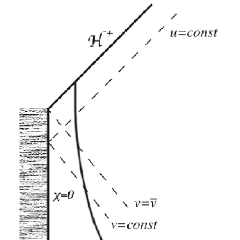
Because the Kruskal coordinates $\cal U$ and $\cal V$ are regular everywhere, they can be matched to $U$ and $V$. In particular, if two nearby outgoing rays differ by ${\rm d}U$ inside the star, then they will also differ outside by ${\rm d}U=\beta({\cal U}){\rm d}{\cal U}$, with $\beta$ being a regular function. By the same token, since $V$ and $v$ are regular everywhere, we have ${\rm d}V=\zeta(v){\rm d}v$, where $\zeta$ is another regular function. In fact, if we consider the last ray $v=\bar{v}$ that passes through the centre of the star before the formation of the horizon, then to first order ${\rm d}V=\zeta(\bar{v}){\rm d}v$, where $\zeta(\bar{v})$ is now constant.

We can write near the horizon

$${\rm d}U=\beta(0)\frac{{\rm d}{\cal U}}{{\rm d}u}{\rm d}u\;.$$ (2.138)

Since for the centre of the star ${\rm d}U={\rm d}V=\zeta(\bar{v}){\rm d}v$, this immediately integrates to

$$\zeta(\bar{v})(v-{\bar{v}})=\beta(0){\cal U}(u)=-\beta(0)\psi^{-1}\left(-u\right)\sim-2\beta(0)\frac{M^{2}}{u}\;.$$ (2.139)

The last approximation follows from Eq. (2.132) where $\xi\sim\psi^{-1}(-2M^{2}/\xi)$ near the horizon.

Thus the late-time worldline for the centre of the star is, finally, represented by the equation 

$$v\sim{\bar{v}}-\frac{A}{u}\;,\quad u\to+\infty\;,$$ (2.140)

where $A=2\beta(0)M^{2}/\zeta(\bar{v})$ is a positive constant that depends on the details of the internal metric and consequently on the dynamics of collapse.

We first note that the worldline (2.140) differs from the one resulting from the collapse of a nonextremal object, which would be of the form (see for example [53, 4, 172])

$$v\sim{\bar{v}}-B{\rm e}^{-\kappa u}\;,\quad u\to+\infty\;.$$ (2.141)

One immediately wonders, then, if our result can be recovered in the case of nonextremal black holes by simply going to a higher order approximation for the asymptotic worldline of the centre of the collapsing star. It is easy to see that this is not the case. Recall that in the Kruskal coordinates ${\cal U}$ and ${\cal V}$, the horizon is located at ${\cal U}=0$. Suppose that the worldline of the centre of the star crosses the horizon at some ${\cal V}=\overline{\cal V}$. Let us expand ${\cal V({\cal U})}$ in a Taylor series around ${\cal U}=0$ such that ${\cal V}=\overline{\cal V}+\alpha_{1}\,{\cal U}+\alpha_{2}\,{\cal U}^{2}$. The term $\alpha_{1}\,{\cal U}\propto{\rm e}^{-\kappa u}$ is the usual one found for the thermal case and $\alpha_{2}\,{\cal U}^{2}$ is the correction. However, ${\cal U}^{2}\propto{\rm e}^{-2\kappa u}$ and so this term is also a constant for extremal incipient black holes. In fact the corrections are constant to arbitrary order. The extremal worldline in no sense, therefore, represents a limit of the nonextremal case but implies a real discontinuity in the asymptotic behaviour of the collapsing object.

Equations (2.140) and (2.141) contain the constants $A$ and $B$, which are determined by the dynamics of collapse. In the non extremal case, it is known that no measurement performed at late times can be used to infer the value of $B$, thus enforcing the no-hair theorems. In particular, the spectrum of Hawking radiation depends only on the surface gravity $\kappa$. It is natural to ask whether a similar statement holds true also for extremal black holes. This point will be analyzed in the following sections.

2.5.3 Bogoliubov coefficients

Let us now consider a test quantum field in the spacetime of an incipient extremal RN black hole. For the sake of simplicity, and without loss of generality, we can restrict our analysis to the case of a hermitian, massless scalar field $\phi$. Instead of dealing with a proper black hole, we consider a two-dimensional Minkowski spacetime with a timelike boundary [53, 4]. This spacetime is described by null coordinates $(u,v)$ and the equation governing the boundary is the same that describes the worldline of the centre of the star, say $v=p(u)$ . At the centre of the star the ingoing modes of $\phi$ become outgoing, and vice versa; this translates into the requirement that at the spacetime boundary there is perfect reflection, or that $\phi(u,p(u))\equiv 0$. Hence, the idea of a “mirror”: the timelike boundary in Minkowski spacetime is traced out by a one-dimensional moving mirror for the field $\phi$.

In general, for a worldline $v=p(u)$ one has ${\rm d}\tau=\sqrt{p^{\prime}(u)}\,{\rm d}u$, where $\tau$ is the proper time along the worldline. From this and the fact that the acceleration for the trajectory in two-dimensional Minkowski spacetime is $a={1\over 2}\sqrt{p^{\prime\prime}(u)^{2}/p^{\prime}(u)^{3}}\$, one can easily check that Eqs. (2.140) and (2.141) yield $a^{2}=1/A$ and $a^{2}=\kappa{\rm e}^{\kappa u}/(4B)$, respectively. Thus we see that an incipient extremal black hole is modeled at late times by a uniformly accelerated mirror; for nonextremal black holes the acceleration of the mirror increases exponentially with time. In both cases the worldline of the mirror has a null asymptote $v=\bar{v}$ in the future, while it starts from the timelike past infinity $i^{-}$ at $t=-\infty$.

Without loss of generality, one can assume that the mirror is static for $t<0$. A suitable worldline is then

$$p(u)=u\Theta(-u)+f(u)\Theta(u)\;,$$ (2.142)

where $\Theta$ is the step function, defined as

$$\Theta(\xi)=\left\{\begin{array}[]{l}1\quad\mbox{if}\quad\xi\geq 0\;,\\ 0\quad\mbox{if}\quad\xi<0\;,\end{array}\right.$$ (2.143)

and $f(u)$ is a function with the asymptotic form (2.140). In order for the worldline to be $C^{1}$, $f(u)$ must be such that $f(0)=0$ and $f^{\prime}(0)=1$ . To simplify calculations, it is convenient to choose $f(u)$ to be hyperbolic at all times [4], i.e.,

$$f(u)=\sqrt{A}-{A\over u+\sqrt{A}}\;,$$ (2.144)

which coincides with the function on the right hand side of Eq. (2.140), up to a (physically irrelevant) translation of the origin of the coordinates.

Due to the motion of the mirror, one expects that the In and Out vacuum states will differ, leading to particle production whose spectrum depends on the function $p(u)$. In our case, because the worldline of the mirror has a null asymptote $v=\bar{v}$ in the future but no asymptotes in the past, the explicit forms of the relevant In and Out modes for $\phi$ are easily shown to be

$$\phi_{\omega}^{\rm(in)}(u,v)={{\rm i}\over\sqrt{4\pi\omega}}\left({\rm e}^{-{\rm i}\omega v}-{\rm e}^{-{\rm i}\omega p(u)}\right)$$ (2.145)

and

$$\phi_{\omega}^{\rm(out)}(u,v)={{\rm i}\over\sqrt{4\pi\omega}}\left({\rm e}^{-{\rm i}\omega u}-\Theta\left(\bar{v}-v\right){\rm e}^{-{\rm i}\omega q(v)}\right)\;,$$ (2.146)

where $q(v)=p^{-1}(v)$ and $\omega>0$. The spectrum of particles created in such a scenario is known although, to our knowledge, no one has pointed out the correspondence with the formation of extremal black holes. However, since the result is something of a textbook case, we here merely summarize the main steps; for details, see for example Ref. [4], p 109.

The In and Out states of $\phi$ can be related by the Bogoliubov coefficients:

$$\alpha_{\omega\omega^{\prime}}=\left(\phi_{\omega}^{\rm(out)},\phi_{\omega^{\prime}}^{\rm(in)}\right)=-{\rm i}\int_{0}^{+\infty}{\rm d}x\left[\phi_{\omega}^{\rm(out)}(u,v)\stackrel{{\scriptstyle\leftrightarrow}}{{\partial}}_{t}\phi_{\omega^{\prime}}^{{\rm(in)}}(u,v)^{\ast}\right]_{t=0}\;;$$ (2.147)

$$\beta_{\omega\omega^{\prime}}=-\left(\phi_{\omega}^{\rm(out)},\phi_{\omega^{\prime}}^{\rm(in)\ast}\right)={\rm i}\int_{0}^{+\infty}{\rm d}x\left[\phi_{\omega}^{\rm(out)}(u,v)\stackrel{{\scriptstyle\leftrightarrow}}{{\partial}}_{t}\phi_{\omega^{\prime}}^{\rm(in)}(u,v)\right]_{t=0}\;.$$ (2.148)

There has been some discussion in the literature [174] about whether the calculation of the Bogoliubov coefficients by Fulling and Davies [53, 4] is correct. We find that their approximations are valid in the asymptotic regime of interest to us.

The spectrum of created particles is given by the expectation value of the “out quanta” contained in the In state, $\langle 0,\mbox{in}|N_{\omega}^{\rm(out)}|0,\mbox{in}\rangle$. In terms of the Bogoliubov coefficients, this spectrum is

$$\langle N_{\omega}\rangle=\int_{0}^{+\infty}{\rm d}\omega^{\prime}\,|\beta_{\omega\omega^{\prime}}|^{2}\;,$$ (2.149)

where $\langle N_{\omega}\rangle$ is a shorthand for $\langle 0,\mbox{in}|N_{\omega}^{\rm(out)}|0,\mbox{in}\rangle$.

With the choice (2.144), one can compute the Bogoliubov coefficients which are appropriate in the asymptotic regime $t\to+\infty$. Performing the integrals in Eqs. (2.147) and (2.148) gives [4]

$$\alpha_{\omega\omega^{\prime}}\approx{\rm i}\frac{\sqrt{A}}{\pi}{\rm e}^{-{\rm i}{\sqrt{A}}(\omega+\omega^{\prime})}K_{1}(2{\rm i}(A\omega\omega^{\prime})^{1/2})\;,$$ (2.150)

$$\beta_{\omega\omega^{\prime}}\approx\frac{\sqrt{A}}{\pi}{\rm e}^{{\rm i}{\sqrt{A}}(\omega-\omega^{\prime})}K_{1}(2(A\omega\omega^{\prime})^{1/2})\;,$$ (2.151)

where $K_{1}$ is a modified Bessel function, shown in Fig. 2. For argument $z$, $K_{1}(z)\sim 1/z$ for $z\to 0$, and $K_{1}(z)\sim\sqrt{\pi/(2z)}\,{\rm e}^{-z}$ when $z\to+\infty$ [175].

Figure 2.2: Plot of the modified Bessel function $K_{1}(z)$, squared.

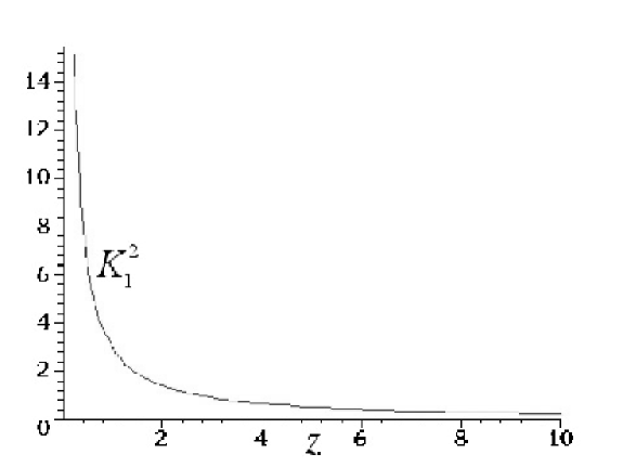
We emphasize that Eqs. (2.150) and (2.151) do not correspond to a full evaluation of the integrals in Eqs. (2.147) and (2.148), but only take into account the contribution for $x\approx\sqrt{A}$, i.e., from the mirror worldline at $u\to+\infty$. This is the only part of the Bogoliubov coefficients that can be related to particle creation by an incipient black hole, because any other contribution corresponds to particles created much earlier, and depends therefore on the arbitrary choice of $p(u)$ in the non-asymptotic regime. Clearly, since $\langle N_{\omega}\rangle\neq 0$, there is particle creation by the incipient extremal RN black hole .

Due to the $1/(\omega\omega^{\prime})$ in the asymptotic form of $|\beta_{\omega\omega^{\prime}}|^{2}$, the spectrum (2.149) diverges at low frequencies. The divergence in $\omega^{\prime}$ has the same origin as the one that appears in the case of non extremal black holes, where

$$|\beta_{\omega\omega^{\prime}}|^{2}=\frac{1}{2\pi\omega^{\prime}}\left(\frac{1}{{\rm e}^{2\pi\omega/\kappa}-1}\right)\;.$$ (2.152)

These Bogoliubov coefficients also contain a logarithmic divergence in $\omega^{\prime}$, which is due to the evaluation of the mode functions at $u=+\infty$ and for that reason can be interpreted as an accumulation of an infinite number of particles after an infinite time. The divergence can be removed, however, as Hawking suggested [176] by the use of wave packets instead of plane-wave In states; this has the effect of introducing a frequency cutoff.

Contrary to what happens in the non extremal case, $\langle N_{\omega}\rangle$ is not a Planckian distribution and therefore the spectrum of created particles is nonthermal. Thus, the notion of temperature is undefined. This result supports the view that an extremal black hole is not the zero temperature limit of a non extremal one. However, it would be premature to base such conclusions only on the basis of Eq. (2.149), because the Bogoliubov coefficients tell us only that particles are created at some time in the late stages of collapse, which does not necessarily mean that such creation takes place at a steady rate.

Noticeably equations (2.149) and (2.151) also indicate that an incipient extremal RN black hole creates particles with a spectrum that depends on the constant $A$. These results immediately raise two problems.

First, since particle creation leads to black hole evaporation, it seems that (some version of) the cosmic censorship conjecture could be violated. Indeed, emission of neutral scalar particles implies a decrease in $M$, while $Q$ remains constant; evidently, a transition to a naked singularity ($Q^{2}>M^{2}$) should take place.

Second, the dependence of the spectrum on $A$, which in turn depends on the details of collapse, raises the possibility of getting information about the collapsing object through measurements performed at late times, a contradiction of the no-hair theorems.

In order to clarify these issues, in the next two sections we shall refine our conclusions through an analysis of the stress-energy tensor of the quantum field.

2.5.4 Preservation of cosmic censorship

We consider here the first of the problems mentioned above. The luminosity of the black hole, the rate of change of $M$, is given by the flux of created particles at infinity, or the $T_{uu}$ component of the stress-energy tensor.

We saw in chapter 1 that the expectation value of $T_{uu}$ for the case of a moving boundary in two-dimensional Minkowski spacetime is given by the Schwartzian derivative of $p(u)$

$$\langle:\!T_{uu}\!:\rangle=\frac{1}{4\pi}\left(\frac{1}{4}\left(\frac{p^{\prime\prime}}{p^{\prime}}\right)^{2}-{1\over 6}\frac{p^{\prime\prime\prime}}{p^{\prime}}\right)\;.$$ (2.153)

where the primes denote derivatives with respect to $u$.

Inserting the form (2.142) of $p$, with $f$ given by Eq. (2.144), into Eq. (2.153), one gets

$$\langle:\!T_{uu}\!:\rangle={1\over 24\pi\sqrt{A}}\,\delta(u)\;.$$ (2.154)

Thus, the only non-vanishing contribution to $\langle:\!T_{uu}\!:\rangle$ is due to the transition from uniform to hyperbolic motion that takes place at $t=0$. For the discussion of incipient black holes, only the behaviour for $u\to+\infty$ is relevant, and so this feature is uninteresting. On the other hand, in the hyperbolic regime $\langle:\!T_{uu}\!:\rangle$ vanishes identically. (It is also straightforward to check from Eq. (2.153) that, conversely, a hyperbolic worldline is the only one with nonzero acceleration that leads to $\langle:\!T_{uu}\!:\rangle=0$.)

This result shows that the flux due to an incipient extremal black hole vanishes asymptotically at late times. Consequently, extremal black holes do not lose mass , and cosmic censorship is preserved. However, the nonzero value of $\beta_{\omega\omega^{\prime}}$ clearly shows that there is particle creation during collapse. Cosmic censorship has apparently been rescued only at the price of introducing a paradox, namely: particles are created and their flux has zero expectation value. How can these two statements be simultaneously true?

This puzzling situation has been extensively discussed in the context of particle emission from a uniformly accelerating mirror [53, 4, 52]. Fulling and Davies [53] explain the net zero energy flux in the presence of nonzero $\beta_{\omega\omega^{\prime}}$ by a special cancellation of the created modes via quantum interference, which is due to contributions from the coefficients $\alpha_{\omega\omega^{\prime}}$. In section 2.5.6 we analyze this issue further by examining the response function of an ideal detector.

2.5.5 Preservation of the no-hair theorems

We now turn to the second of the problems mentioned earlier: given that the spectrum contains the constant $A$, do extremal black holes violate the no-hair theorems? The result $\langle:\!T_{uu}\!:\rangle=0$ suggests an escape — in spite of the nonzero value of $\langle N_{\omega}\rangle$, no radiation is actually detected. However, this resolution raises new questions. If no radiation is detected, how can one claim that the black hole emits anything at all? Is the radiation observable? How should one then interpret $\langle N_{\omega}\rangle$?

It is premature to claim that no radiation is detected only on the basis of $\langle:\!T_{uu}\!:\rangle=0$, because there could be other nonvanishing observables from which one might infer the presence of quanta. A straightforward calculation shows that the expectation values of $T_{vv}$ and $T_{uv}$ are also zero. However, let us examine the variance $\Delta T_{uu}$ of the flux. Wu and Ford [173] have also recently given the following expression for $\langle:\!T^{2}_{uu}\!:\rangle$ in the case of a minimally coupled, massless scalar field in two-dimensional Minkowski spacetime with a timelike boundary described by the equation $v=p(u)$:

$$\langle:\!T^{2}_{uu}\!:\rangle=\frac{1}{\left(4\pi\right)^{2}}\left(-\frac{4p^{\prime 2}}{(v-p(u))^{4}}+\frac{3}{16}\left(\frac{p^{\prime\prime}}{p^{\prime}}\right)^{4}-\frac{1}{4}\frac{p^{\prime\prime\prime}}{p^{\prime}}\left({p^{\prime\prime}\over p^{\prime}}\right)^{2}+{1\over 12}\left({p^{\prime\prime\prime}\over p^{\prime}}\right)^{2}\right)\;.$$ (2.155)

If one ignores the so-called cross terms [173], this coincides with the variance $\Delta T_{uu}$ (because in our case $\langle:\!T_{uu}\!:\rangle=0$). With $p$ given by Eqs. (2.142) and (2.144), Eq. (2.155) gives, for $u>0$,

$$\langle:\!T^{2}_{uu}\!:\rangle=-{A^{2}\over 4\pi^{2}\left(A+\left(v-\bar{v}\right)u\right)^{4}}\sim-{A^{2}\over 4\pi^{2}\left(v-\bar{v}\right)^{4}u^{4}}\;.$$ (2.156)

Thus, in spite of the fact that the expectation value of the flux vanishes identically, its statistical dispersion does not, but its value becomes smaller and smaller and tends to zero in the limit $u\to+\infty$. Hence, although one could in principle infer the value of the constant $A$ by measuring the quantity $\Delta T_{uu}$ at late times, such measurements will become more and more difficult as $\Delta T_{uu}$ decreases according to Eq. (2.156). This damping is of course reminiscent of the familiar damping of perturbations, which prevents one from detecting by late-time measurements the details of an object that collapses into a black hole [98]. Therefore, monitoring $\Delta T_{uu}$ does not lead to a violation of the no-hair theorems, because no trace of $A$ will survive in the limit $u\to+\infty$.

This discussion shows only that no violation of the no-hair theorems can be detected by measuring the variance in the energy flux. The possibility remains that other types of measurement could allow one to find out the value of $A$. If, however, $\Delta T_{\mu\nu}\to 0$ for $u\to+\infty$, then the random variable $T_{\mu\nu}$ must tend to its expectation value, i.e., to zero. This means that, asymptotically, the properties of the field are those of the vacuum state. Consequently, all local observables will tend to their vacuum value.

Although extremal black holes obey the no-hair theorems, the way in which cosmic baldness is enforced differs from the non extremal situation. Consider again the variance of the flux. Inserting the function $p$ for non extremal incipient black holes (see Eq. (2.141)) into Eqs. (2.153) and (2.155), one gets $\langle:\!T_{uu}\!:\rangle=\kappa^{2}/(48\pi)$ and

$$\langle:\!T_{uu}^{2}\!:\rangle={1\over(4\pi)^{2}}\left({\kappa^{4}\over 48}-{4\kappa^{2}B^{2}{\rm e}^{-2\kappa u}\over\left(v-\bar{v}+B{\rm e}^{-\kappa u}\right)^{4}}\right)\sim{\kappa^{4}\over 768\pi^{2}}-{\kappa^{2}B^{2}{\rm e}^{-2\kappa u}\over 4\pi^{2}\left(v-\bar{v}\right)^{4}}\;.$$ (2.157)

Contrary to the extremal case, the “non extremal” variance $\Delta T_{uu}$ tends not to zero as $u\to+\infty$, but to the value $\kappa^{2}\sqrt{2}/(48\pi)$, which corresponds to thermal emission; this is sufficient to guarantee that no information about the details of collapse is conveyed. Furthermore, the approach to this value is exponentially fast, while for the extremal configuration the decay obeys only a power law.

2.5.6 Detecting radiation from a uniformly accelerated mirror

In Sec. 2.5.4 we mentioned the apparently paradoxical situation in which nonzero particle production (as shown by non-vanishing Bogoliubov coefficients $\beta_{\omega\omega^{\prime}}$) is accompanied by zero energy flux (vanishing expectation value of the stress-energy-momentum tensor.) Discussions about such issues are often phrased in terms of ideal detectors [4, 32]. Although our previous arguments are based solely on the behaviour of the stress-energy-momentum tensor, we can gain some additional insight into the “paradox” by considering the response of a simple monopole detector on a geodesic worldline $v=u+2x_{0}$, with $x_{0}=\mbox{const}$, in two-dimensional Minkowski spacetime.

We are interested in computing the detector response function per unit time, defined as

$${\cal R}(E)=\lim_{T\to+\infty}{1\over 2T}\int_{-T}^{T}{\rm d}\tau\int_{-T}^{T}{\rm d}\tau^{\prime}\,\Theta(E){\rm e}^{-{\rm i}E(\tau-\tau^{\prime})}D^{+}(u(\tau),v(\tau);u(\tau^{\prime}),v(\tau^{\prime}))\;,$$ (2.158)

where $D^{+}$ is the Wightman function of the scalar field in the In vacuum, $u(\tau)=\tau-x_{0}$, $v(\tau)=\tau+x_{0}$, and $E$ is the excitation energy of the detector. (Note that $E\geq 0$, which is automatically enforced by the presence of the step function $\Theta(E)$ on the right hand side of Eq. (2.158).) In terms of the In modes, $D^{+}$ has the form

$$D^{+}(u,v;u^{\prime},v^{\prime})=\int_{-\infty}^{+\infty}{\rm d}\omega\,\Theta(\omega)\phi_{\omega}^{\rm(in)}(u,v)\phi_{\omega}^{\rm(in)}(u^{\prime},v^{\prime})^{\ast}\;,$$ (2.159)

where we have extended the integration range to $-\infty$, by introducing the step function $\Theta(\omega)$.

Since the definition of ${\cal R}(E)$ involves an integration over time from $-\infty$ to $+\infty$, in the case of a mirror worldline of the type (2.142) it will get contributions corresponding to the nonzero flux (such as, for example, the one at $u=0$ when $f(u)$ is given by Eq. (2.144)). These we regard as spurious, because we are really interested in clarifying the relationship between zero flux and nonzero spectrum in the hyperbolic regime. For this reason, let us consider a mirror worldline which is hyperbolic at all times, say $p(u)=-A/u$ for $u>0$, for which there can be no such spurious contributions to ${\cal R}(E)$.

The worldline $p(u)=-A/u$ has a null asymptote in the past, thus

$$\phi_{\omega}^{\rm(in)}(u,v)={{\rm i}\over\sqrt{4\pi\omega}}\left({\rm e}^{-{\rm i}\omega v}-\Theta(u){\rm e}^{-{\rm i}\omega p(u)}\right)\;.$$ (2.160)

The former expression does not form a complete basis in the presence of a past null asymptote but it takes into account only those outgoing modes which have been reflected by the moving mirror. On substituting Eq. (2.160) into Eq. (2.159), we have

$$D^{+}(u,v;u^{\prime},v^{\prime})=F_{1}(v,v^{\prime})+F_{2}(u,v^{\prime})+F_{3}(v,u^{\prime})+F_{4}(u,u^{\prime})\;,$$ (2.161)

where:

$$F_{1}(v,v^{\prime})={1\over 4\pi}\int_{-\infty}^{+\infty}{\rm d}\omega\,{\Theta(\omega)\over|\omega|}\,{\rm e}^{-{\rm i}\omega(v-v^{\prime})}\;;$$ (2.162)

$$F_{2}(u,v^{\prime})=-{1\over 4\pi}\Theta(u)\int_{-\infty}^{+\infty}{\rm d}\omega\,{\Theta(\omega)\over|\omega|}\,{\rm e}^{{\rm i}\omega(v^{\prime}-p(u))}\;;$$ (2.163)

$$F_{3}(v,u^{\prime})=-{1\over 4\pi}\Theta(u^{\prime})\int_{-\infty}^{+\infty}{\rm d}\omega\,{\Theta(\omega)\over|\omega|}\,{\rm e}^{-{\rm i}\omega(v-p(u^{\prime}))}\;;$$ (2.164)

$$F_{4}(u,u^{\prime})={1\over 4\pi}\Theta(u)\Theta(u^{\prime})\int_{-\infty}^{+\infty}{\rm d}\omega\,{\Theta(\omega)\over|\omega|}\,{\rm e}^{-{\rm i}\omega(p(u)-p(u^{\prime}))}\;.$$ (2.165)

Correspondingly, ${\cal R}(E)$ can be split into four parts: ${\cal R}(E)={\cal R}_{1}(E)+{\cal R}_{2}(E)+{\cal R}_{3}(E)+{\cal R}_{4}(E)$.

The terms ${\cal R}_{1}(E)$, ${\cal R}_{2}(E)$, and ${\cal R}_{3}(E)$ can be computed straightforwardly, by using the formal identities

$$\lim_{T\to+\infty}\int_{-T}^{T}{\rm d}\tau\,{\rm e}^{{\rm i}\xi\tau}=2\pi\delta(\xi)$$ (2.166)

and

$${1\over|E|}\,\Theta(E)\Theta(-E)=2\delta(E)\;,$$ (2.167)

the latter being easily established by considering the sequence of functions $(|E|+\epsilon)^{-1}\Theta(E+\epsilon)\Theta(-E+\epsilon)$ in the limit $\epsilon\to 0$. We get ${\cal R}_{1}(E)=-2{\cal R}_{2}(E)=-2{\cal R}_{3}(E)=\delta(E)$, and so the first three contributions to ${\cal R}(E)$ sum to zero.

The computation of ${\cal R}_{4}(E)$ is cleaner if one works in dimensionless variables, such as $\widetilde{E}=\sqrt{A}\,E$, $\tilde{\omega}=\sqrt{A}\,\omega$, $\tilde{\tau}=\tau/\sqrt{A}$. The identity

$$\int_{0}^{+\infty}{\rm d}\tilde{\omega}\,{{\rm e}^{-{\rm i}\tilde{\omega}(\xi-{\rm i}0)}\over\tilde{\omega}}=-\ln\left(\xi-{\rm i}0\right)+I-{\rm i}\,{\pi\over 2}\;,$$ (2.168)

where $I$ is the divergent quantity

$$I=\int_{0}^{+\infty}{\rm d}\tilde{\omega}\,{\cos\tilde{\omega}\over\tilde{\omega}}\;,$$ (2.169)

together with the properties of the logarithm, allows us to write

$$\int_{-\infty}^{+\infty}{\rm d}\tilde{\omega}\,{\Theta(\tilde{\omega})\over|\tilde{\omega}|}\,\exp\left(-{\rm i}\tilde{\omega}{\tilde{\tau}-\tilde{\tau}^{\prime}\over\left(\tilde{\tau}-\tilde{x}_{0}\right)\left(\tilde{\tau}^{\prime}-\tilde{x}_{0}\right)}\right)=\int_{-\infty}^{+\infty}{\rm d}\tilde{\omega}\,{\Theta(\tilde{\omega})\over|\tilde{\omega}|}\,{\rm e}^{-{\rm i}\tilde{\omega}\left(\tilde{\tau}-\tilde{\tau}^{\prime}\right)}$$

$$-\int_{-\infty}^{+\infty}{\rm d}\tilde{\omega}\,{\Theta(\tilde{\omega})\over|\tilde{\omega}|}\,{\rm e}^{-{\rm i}\tilde{\omega}\left(\tilde{\tau}-\tilde{x}_{0}\right)}-\int_{-\infty}^{+\infty}{\rm d}\tilde{\omega}\,{\Theta(\tilde{\omega})\over|\tilde{\omega}|}\,{\rm e}^{{\rm i}\tilde{\omega}\left(\tilde{\tau}^{\prime}-\tilde{x}_{0}\right)}+2I\;.$$ (2.170)

In this expression we have replaced one of the quantities $I-{\rm i}\pi/2$ with its complex conjugate by simultaneously changing the sign in one of the exponents. This manipulation is allowed by the fact that, since $\tilde{\tau}-\tilde{x}_{0}$ and $\tilde{\tau}^{\prime}-\tilde{x}_{0}$ can never become negative in $F_{4}$, their logarithms are always real. Note that the resulting expression agrees with the property of ${\cal R}(E)$ being a real quantity.

We can thus write ${\cal R}_{4}(E)={\cal R}_{41}(E)+{\cal R}_{42}(E)+{\cal R}_{43}(E)+{\cal R}_{44}(E)$. Using the formal relations

$$\lim_{\widetilde{T}\to+\infty}\int_{\tilde{x}_{0}}^{\widetilde{T}}{\rm d}\tilde{\tau}\,{\rm e}^{{\rm i}\xi\tilde{\tau}}=\pi\delta(\xi)+{\rm i}{\rm e}^{{\rm i}\,\xi\tilde{x}_{0}}\,{\mathcal{P}}\left(1\over\xi\right)\;,$$ (2.171)

and

$$\lim_{\widetilde{T}\to+\infty}{1\over\widetilde{T}}\int_{\tilde{x}_{0}}^{\widetilde{T}}{\rm d}\tilde{\tau}\,{\rm e}^{{\rm i}\xi\tilde{\tau}}=\Theta(\xi)\Theta(-\xi)\;,$$ (2.172)

together with Eq. (2.167), we get ${\cal R}_{41}(E)=\delta(E)/4$, ${\cal R}_{42}(E)+{\cal R}_{43}(E)=-\delta(E)/2$, and ${\cal R}_{44}(E)=I\delta(E)/4$. Finally, since $I$ is divergent we can write

$${\cal R}(E)={I\over 4}\,\delta(E)\;.$$ (2.173)

Thus, we have essentially a delta function peaked at zero energy. Now, ${\cal R}(E)$ is related to a quantum mechanical probability and so this result means that, for any value $E>0$ of the energy, no matter how small, the detector has probability 1 of making a transition of amplitude smaller that $E$ and probability 0 of detecting particles of higher energy. (Of course, this does not mean that it will never make transitions with $E>0$; only that these take place with probability 0.) The reason for this behaviour is evidently the divergence in the spectrum as $\omega\to 0$. Of course, the detector does not gain energy during such a “detection” — in fact, one can say that there is no detection at all. This is compatible with the zero value of the flux and moreover it is also in agreement with what should be expected from the Bogoliubov coefficient (2.151) which in the low frequency limit loses any dependence on $A$

$$\lim_{\omega\to 0}|\beta|^{2}\approx\frac{1}{(4\pi)^{2}}\frac{1}{\omega}{\omega^{\prime}}.$$ (2.174)

Hence one might be tempted to call the particles emitted by a mirror in hyperbolic motion “phantom radiation”: because only arbitrarily soft particles would be registered by the detector with any nonzero probability, there would be no chance of determining the spectrum $\langle N_{\omega}\rangle$. The question arises therefore, of whether there is any way to screen our detector from this overwhelming flux of soft quanta.

One might think of acting on the selectivity of the detector by using a two level system that requires at least a minimal energy to switch. Unfortunately, the detection of the infinite tail of soft quanta corresponds to the “transition” from the ground state to the ground state, and there is obviously no way to forbid this process. The detector cannot be forbidden not to switch!

Therefore the analysis of the response function of a detector also seems to prove that the radiation from uniformly accelerated mirrors (and extremal incipient black holes) is in some sense like the apple in Dante’s purgatory: We can see it with our mind but we shall never have it in our hands …

2.5.7 Conclusions

We have just seen how, in a subtle way indeed, cosmic censorship and the no hair theorem are preserved in the formation of an extremal black hole. In fact, although they appear to emit particles, closer scrutiny reveals that the flux of emitted radiation vanishes identically, and in the limit $t\to+\infty$ any measurement of local observables gives results indistinguishable from those in the vacuum state. This is not incompatible with a nonzero spectrum, which is not a local quantity and tells us only that particles are created at some time during collapse (not necessarily at $t=+\infty$). Thus, extremal black holes are not pathological in this respect.

However, we have seen that there are several clearly defined senses in which non extremal and extremal black holes differ. In fact the conclusions which we can derive from the above results are even more radical. Not only do they appear to involve a fundamental difference in the behaviour of the radiation emitted by non-extremal and extremal black holes but also they converge towards a picture where our understanding of the third law of black hole thermodynamics is heavily transformed.

A first set of conclusions is related to the nature of the quantum radiation from the incipient extremal black holes. Information lost to an external observer depends on the rate at which the statistical dispersion of the flux approaches its value for $t\to+\infty$. In the non extremal case, the dispersion goes to zero exponentially fast, Eq. (2.157), whereas for an incipient extremal black hole it follows a slower power law, given by Eq. (2.156). More importantly, for $Q^{2}\to M^{2}$, Eq. (2.156) is not the limit of Eq. (2.157). One cannot therefore, consider quantum emission by an incipient extremal black hole to be the limiting case of emission by a non extremal black hole.

In particular, although at $t=+\infty$ a black hole with $Q^{2}=M^{2}$ is totally quiescent it would be incorrect to consider it as the thermodynamic limit of a non extremal black hole, that is, an object at zero temperature. Indeed, the quantum radiation emitted by an incipient extremal black hole is not characterized by a temperature at any time during collapse. Whereas incipient non extremal black holes have a well defined thermodynamics, this is not true for extremal holes, and they should be considered as belonging to a different class. This result suggests that any calculations that implicitly rely on a smooth limit in thermodynamic quantities at $Q^{2}=M^{2}$ are suspect, if not incorrect. Our conclusions, of course, are just pertinent to incipient black holes; extending them to eternal black holes seems plausible, but requires care. (Even at the classical level, eternal black holes must be regarded as fundamentally different from those deriving from collapse, because the global structure of spacetime differs in the two cases.)

Moreover it should be stressed that remarkably our calculations lead to the conclusion that extremal black holes are substantially impossible to obtain in a semiclassical approach. We have seen in Sec. 2.5.4 that if $Q^{2}=M^{2}$ at the onset of the hyperbolic worldline (2.140), it will remain so and the cosmic censorship conjecture is preserved. However, the fact that mass loss from an incipient extremal black hole is zero only in the late hyperbolic stage seems to imply that an enormous fine tuning is required in order to produce an extremal object by means of gravitational collapse. In fact, an object that is extremal from the start of its collapse might be unstable with respect to transition to a configuration with $Q^{2}>M^{2}$. Such a transition would be triggered by quantum emission in the early phases of collapse, when $p(u)$ has not yet assumed its hyperbolic form. This raises the question of how, in the presence of quantum radiation, the formation of a naked singularity is prevented (for example, by the emission of charged particles) and the cosmic censorship conjecture preserved.

A second set of conclusions has a more strictly thermodynamical relevance. We have seen in section 2.4 how the extremal solution appears to be “totally disconnected” from the thermodynamical behaviour of the non-extremal one: the different topology puts them in different categories and does not allow any well defined limit between the two. Adding these facts to our results, one may conjecture that the unattainability formulation of the third law for black hole thermodynamics is actually implemented in an unexpected way: the temperature of a black hole cannot be reduced to zero simply because no black hole zero temperature state exists.

This conjecture, although it might appear very radical, it is not as dramatic as it might seem. In standard thermodynamics the absence of zero-temperature states is not a pathology. Indeed a well-defined thermodynamics can be defined without them.

It is alternatively possible that to avoid the above conclusion one should use a more sophisticated theory. Noticeably the divergence of the particle spectrum $\langle N_{\omega}\rangle$ is reminiscent of the infrared catastrophe typical of QED, which manifests itself, for instance, in the process of Bremsstrahlung (see, for example, Ref. [177], pp. 165–171). However, the infrared divergence in the Bremsstrahlung cross section produces no observable effect, because it is canceled by analogous terms coming from radiative corrections. (Thanks to the Bloch–Nordsieck theorem, this cancellation is effective to all orders of perturbation theory.) One may well wonder whether the $\omega=0$ singularity in our spectrum is similarly fictitious and could thus be removed by analogous techniques.

For the mirror this is possible, in principle, if one allows momentum transfer from the field $\phi$ to the mirror, although such a calculation is beyond the scope of the present investigation. (See Ref. [178] for a model that includes recoil.) However, whatever the answer to the mirror problem might be, it does not seem that one could transfer it in any straightforward way to the case of an incipient black hole. Indeed, taking recoil into account would amount to admitting that backreaction is important and that the test-field approximation is never valid. Thus, the whole subject would have to be reconsidered within an entirely different framework.

Nevertheless a recent paper by Anderson, Hiscock and Taylor [179] should be quoted where it is demonstrated that for static RN geometries, zero-temperature black holes cannot exist if one considers spacetime perturbations due to the back-reaction of quantum fields. This seems to imply that even the inclusion of back-reaction is insufficient to impart thermal properties to extremal black holes.

Apparently then, extremal black holes are either physical states which are outside of black hole thermodynamics or they represent solutions in which the external field approach to the semiclassical theory of gravity breaks down. In both cases they would be dramatically different objects from their non-extremal counterparts.

Chapter 3 Toward experimental semiclassical gravity: Acoustic horizons

L’acqua che tocchi de’ fiumi è l’ultima di quella che andò

e la prima di quella che viene.

Così il tempo presente.

Leonardo da Vinci

This chapter is the first of two in which we shall deal with possible experimental tests of particle production from the quantum vacuum. Here we shall study a hydrodynamical system which can closely resemble General Relativity and which can lead to indirect tests of Hawking radiation. In particular we shall devote special attention to the actual realizability of fluid configurations which would be able to simulate event horizons and hence fluxes of Hawking (phonon) radiation. In the subsequent chapter we shall present a tentative explanation of the observed emitted radiation of Sonoluminescence as a manifestation of a dynamical Casimir effect.

3.1 Seeking tests of the dynamical Casimir effect

It is often true that in theoretical physics the elegance and clarity of a formula is judged by its property of relying on a few fundamental constants of nature and basic numbers. In this sense the formula describing the temperature in the Hawking–Unruh effect is in an extremely impressive combination of simplicity and “interdisciplinarity”

$$T=\frac{\hbar}{2\pi ck_{\mathrm{B}}}\cdot a$$ (3.1)

In this formula we find together a geometrical constant $\pi$, the Planck constant of the quantum world, the Boltzmann constant of thermodynamical laws and the speed of light of Special Relativity. The acceleration $a$ appearing above is itself a combination of fundamental quantities in the case of a black hole. In fact it is then equal to the surface gravity $\kappa$ which is, in the Schwarzschild solution, equal to

$$a=\kappa=\frac{c^{4}}{4G_{\mathrm{N}}M}$$ (3.2)

So even the Newton constant of gravitation enters into the count.

This peculiar concentration of fundamental constants is much more than a curiosity. It is indeed a sign of the fact that the effects under considerations must arise from some very simple common background and that this background should be identified in a region of investigation where quantum effects, thermodynamics and fundamental forces meet.

This is a broad field and hence different lines of investigation can be pursued. The realization of this is indeed at the basis of the concrete possibility for us to test this class of effects and to improve our understanding of their role in semiclassical quantum gravity.

In fact it is easy to realize that no “direct” experimental test of the Hawking–Unruh effect will probably be obtainable in the near future. In the cgs system Eq. (3.1) takes the form

$$T=4\times 10^{-23}\frac{\mathrm{K}s^{2}}{\mathrm{cm}}\cdot a$$ (3.3)

This implies that at least an acceleration of order $10^{23}{\mathrm{g}}_{\oplus}$ is required for obtaining a thermal spectrum at only one Kelvin!

Similarly, for a black hole to have a Hawking temperature of the order of one Kelvin requires it to have a mass no greater than $M_{\mathrm{critical}}\approx 10^{15}g$, that is a mass of the order of a common mountain (giving a hadron-sized black hole). Although it is indeed plausible that such objects might form in the very early universe, it is extremely unlikely that we shall “meet” them in the near future.

It is then legitimate to ask if we can test these effects indirectly by concentrating our attention on other possible areas where the production of particles from the quantum vacuum by a time varying external field can come into action. In a certain sense we can aim to test the paradigm at the basis of the Hawking–Unruh effect instead of the effect itself.

We shall see how this research will be not just a useful phenomenological study, but also an extremely powerful tool for investigating some fundamental questions about the deeper nature of the Hawking–Unruh effect and its role as a bridge towards quantum gravity.

3.2 Acoustic Manifolds

It is really true that sometimes deep and fundamental physical answers can be gained by apparently very simple and basic investigations. In this sense few other subjects are comparable to the study of the acoustic manifolds. As we shall see, the answer to the apparently trivial problem of describing the propagation of acoustic disturbances in a non-homogeneous flowing fluid has revealed a deep analogy with Lorentzian differential geometry [180, 181, 182, 183, 184, 185, 186]. This analogy is at the root of the possibility to conceive experiments to finally test semiclassical quantum gravity effects such as the Hawking–Unruh one. However, let us take a step back and pursue an ab initio discussion of the subject.

As a first approach to the problem we can start with a hydrodynamical system characterized by a few fundamental quantities: a density $\rho$, a velocity field ${\mathbf{v}}$ and a pressure $p$. This system is characterized by the standard equations of fluid dynamics, that is

• The continuity equation

  $${\partial\rho\over\partial t}+\vec{\nabla}\cdot\left(\rho\,{\mathbf{v}}\right)=0,$$ (3.4)

• and the Euler equation

  $$\rho\;{\mathbf{a}}={\mathbf{f}},$$ (3.5)

  where ${\mathbf{a}}$ is the fluid acceleration,

  $${\mathbf{a}}={\partial{\mathbf{v}}\over\partial t}+({\mathbf{v}}\cdot\vec{\nabla}){\mathbf{v}},$$ (3.6)

  and ${\mathbf{f}}$ stands for the force density, the sum of all forces acting on the fluid per unit volume.

We shall assume that all of the external forces are gradient-derived (possibly time-dependent) body forces, which for simplicity we collect together in a generic term $-\rho\vec{\nabla}\Phi$. In addition to the external forces, ${\mathbf{f}}$ contains a contribution from the pressure of the fluid and, possibly, a term coming from the kinematic viscosity $\nu$ . Thus, equation (3.5) takes the Navier–Stokes form

$$\rho\left({\partial{\mathbf{v}}\over\partial t}+({\mathbf{v}}\cdot\vec{\nabla}){\mathbf{v}}\right)=-\vec{\nabla}p-\rho\;\vec{\nabla}\Phi+\rho\,\nu\,\left(\nabla^{2}{\mathbf{v}}+\frac{1}{3}\vec{\nabla}(\vec{\nabla}\cdot{\mathbf{v}})\right).$$ (3.7)

In our derivation we are going to make a number of technical assumptions in order to have an analytically tractable system.

1. The first assumption is that we have a vorticity-free flow, i.e., that $\vec{\nabla}\times{\mathbf{v}}={\mathbf{0}}$. This condition is generally fulfilled by the superfluid components of physical superfluids. It also implies the possibility to completely specify the velocity of the fluid via a scalar field $\psi$ defined as ${\mathbf{v}}=\vec{\nabla}\psi$.

2. The second assumption is that the fluid has a barotropic equation of state, that is, the density $\rho$ is a function only of the pressure $p$, so

   $$\rho=\rho(p).$$ (3.8)

   We shall consequently define the speed of sound as

   $$c_{\mathrm{s}}^{2}={{\mathrm{d}}p\over{\mathrm{d}}\rho}.$$ (3.9)

   This assumption is crucial because thanks to it the continuity and Euler equations form a complete set of equations — if $p$ is not just a function of $\rho$ one would need an energy equation as well.

3. A third assumption, often made in the existing literature on acoustic geometries, is that of a viscosity-free flow. Although this is quite a realistic condition for superfluids , we shall find that viscosity can in general play a prominent role. For the moment we shall take it to be zero but we shall come back to the issue later.

The system equations (3.4) and (3.7) can be shown to be closed and hence we can always find an exact solution of them $[\rho_{0}(t,{\mathbf{x}}),p_{0}(t,{\mathbf{x}}),\psi_{0}(t,{\mathbf{x}})]$. If we want to describe the propagation of some acoustic perturbations, we can use such a solution as a background and ask how linearized fluctuations of it behave. We can then write

$$\rho(t,{\mathbf{x}}) = \rho_{0}(t,{\mathbf{x}})+\epsilon\;\rho_{1}(t,{\mathbf{x}})+\cdots,$$ (3.10)

$$p(t,{\mathbf{x}}) = p_{0}(t,{\mathbf{x}})+\epsilon\;p_{1}(t,{\mathbf{x}})+\cdots,$$ (3.11)

$$\psi(t,{\mathbf{x}}) = \psi_{0}(t,{\mathbf{x}})+\epsilon\;\psi_{1}(t,{\mathbf{x}})+\cdots.$$ (3.12)

Inserting these forms into the equations of motion (3.4) and (3.7), one finds that the equations for these fluctuations are

$${\partial\rho_{1}\over\partial t}+\nabla\cdot\big{(}\rho_{1}\nabla\psi_{0}+\rho_{0}\nabla\psi_{1}\big{)} = 0,$$ (3.13)

$$\rho_{0}\left({\partial\psi_{1}\over\partial t}+\nabla\psi_{0}\cdot\nabla\psi_{1}\right) = p_{1},$$ (3.14)

$$p_{1} = c_{\mathrm{s}}^{2}\rho_{1}.$$ (3.15)

The same information contained in these three first-order partial differential equations can be assembled into one second-order partial differential equation which takes the (apparently more unpleasant) form

$${\partial\over\partial t}\left[\frac{\rho_{0}}{c_{\mathrm{s}}^{2}}\left({\partial\psi_{1}\over\partial t}+{{\mathbf{v}}}_{0}\cdot\nabla\psi_{1}\right)\right]=\nabla\cdot\left[\rho_{0}\nabla\psi_{1}-\frac{{{\mathbf{v}}}_{0}\rho_{0}}{c_{\mathrm{s}}^{2}}\left({\partial\psi_{1}\over\partial t}+{{\mathbf{v}}}_{0}\cdot\nabla\psi_{1}\right)\right].$$ (3.16)

This is a partial differential equation just in $\psi_{1}(t,x)$ with coefficients depending on the background field around which we are studying the perturbations. Once the equation is solved in $\psi_{1}$ the corresponding values of $\rho_{1}$ and $p_{1}$ follow from the linearized Euler equations and from the equation of state.

So far there is nothing new or strange, but now a surprise appears. If we introduce four-dimensional coordinates in the usual way $x^{\mu}\equiv(t,{\mathbf{x}})$ and a $4\times 4$ matrix

$$g^{\mu\nu}(t,{\mathbf{x}})\equiv{1\over\rho_{0}c_{\mathrm{s}}}\left[\matrix{-1&\vdots&-{\rm v}_{0}^{j}\cr\cdots\cdots&\cdot&\cdots\cdots\cdots\cdots\cr-{\rm v}_{0}^{i}&\vdots&(c_{\mathrm{s}}^{2}\delta^{ij}-{\rm v}_{0}^{i}{\rm v}_{0}^{j})\cr}\right]$$ (3.17)

Then the rather formidable-looking second-order partial differential equation for $\psi_{1}$ can be very simply written as

$${1\over\sqrt{-g}}\;{\partial\over\partial x^{\mu}}\left(\sqrt{-g}\;g^{\mu\nu}\;{\partial\over\partial x^{\nu}}\psi_{1}\right)=0.$$ (3.18)

where we have defined

$$g=\left[\det\left(g^{\mu\nu}\right)\right]^{-1}.$$ (3.19)

It is easy to see that the differential operator appearing in Eq. (3.18) it is just the d’Alembertian built with the inverse metric $g^{\mu\nu}(t,{\mathbf{x}})$. Therefore Eq. (3.18) is exactly the equation of motion of a minimally coupled scalar field propagating in a spacetime with inverse metric $g^{\mu\nu}(t,{\mathbf{x}})$ !

It is interesting to note that Eq. (3.16) does not uniquely fix the equation of motion of $\psi_{1}$. Actually it identifies a class of conformally related solutions. So we could, in principle, take a metric which is conformally related to those given in Eq. (3.17), the price to pay for this would be a more complicated equation for $\psi_{1}$ which would have the same d’Alembertian and some non-minimal coupling.

Comment: One may wonder whether this “geometrical interpretation” of the propagation of acoustic perturbations, has just a formal value or is indeed a true built-in property of hydrodynamics. A first check of this can be to ask whether the equations of motion of ${\mathbf{v}}_{1}$, $\rho_{1}$ and $p_{1}$ are all of the form $\kern 0.5pt{\lower 0.1pt\vbox{\hrule height=0.5pt,width=6.8pt\hbox{\vrule width=0.5pt,height=6.0pt\kern 6.0pt\vrule width=0.3pt} \hrule height=0.3pt,width=6.8pt}}\kern 1.5ptX+\cdots$ where $X$ is any one of the above quantities and       is the d’Alembertian appearing in Eq.(3.18) and defined via the metric (3.20). It is actually possible to check that this is the case. This equality of the d’Alembertians appearing in the equations of motion of all of the physical perturbations, implies that all investigations which are based on the study of the Green functions of the fields (such as, for example, the treatment of Hawking radiation) can be performed using the “trivial” equation for $\psi_{1}$. The basic results can be considered valid also for the (easier to detect) perturbations in $\rho$.

Let us summarise the situation. We have started with a classical hydrodynamical system in flat space and have found that the equations describing the propagation of perturbations can be cast in a form which is manifestly the propagation of a scalar field in a $(3+1)$–dimensional Lorentzian (pseudo-Riemannian) geometry described by what we can call an acoustic metric $g_{\mu\nu}(t,{\mathbf{x}})$.

$$g_{\mu\nu}(t,{\mathbf{x}})\equiv{\rho_{0}\over c_{\mathrm{s}}}\left[\matrix{-(c_{\mathrm{s}}^{2}-{\rm v}_{0}^{2})&\vdots&-{\rm v}_{0}^{j}\cr\cdots\cdots\cdots\cdots&\cdot&\cdots\cdots\cr-{\rm v}_{0}^{i}&\vdots&\delta_{ij}\cr}\right].$$ (3.20)

Note that, although the underlying physics is non-relativistic (one can safely consider $c\approx\infty$ in this sort of problems), we can see that the fluctuations are nevertheless experiencing a full spacetime metric in which exits a group of Lorentz transformations where the role of the speed of light is played by the speed of sound $c_{\mathrm{s}}$. On one hand the fluid particles couple only to the physical (flat) spacetime metric $\eta_{\mu\nu}\equiv(\mbox{diag}[-c^{2},1,1,1])_{\mu\nu}$. On the other hand the sound waves do not experience this “physical metric” and instead couple to the acoustic metric $g_{\mu\nu}$.

In spite of this, it has to be stressed that the hydrodynamical system which we found is far from being equivalent to General Relativity. In fact the acoustic metric depends algebraically on the distribution of matter (the density, velocity of the flow and local speed of sound in the fluid) and it is governed by the fluid equations of motion which constrain the background geometry. In Einstein gravity, the spacetime metric is instead related to the distribution of matter by the non-linear Einstein–Hilbert differential equations.

This difference is also confirmed by looking at the degrees of freedom of these theories. In a completely general $(3+1)$–dimensional Lorentzian geometry the metric has six degrees of freedom (it is described by a $4\times 4$ symmetric matrix which gives $10$ independent components from which one has to subtract the $4$ coordinate conditions). In contrast an acoustic metric is completely specified by the three scalars $\rho_{0}(t,{\mathbf{x}}),\psi_{0}(t,{\mathbf{x}}),c_{\mathrm{s}}(t,{\mathbf{x}})$ so it has at most 3 degrees of freedom per point in spacetime. Considering also the continuity equations, these are further reduced to 2 (for $\psi_{0}(t,{\mathbf{x}})$ and $c_{\mathrm{s}}(t,{\mathbf{x}})$).

Comment: We want here to suggest the idea that a more complex fluid could actually be built in order to have six degrees of freedom per point. The most straightforward way to do this might be to define a “fluid” whose pressure is a tensor $p_{ij}$ so that the barotropic equation has the form: $$p_{ij}=c_{\mathrm{s}}^{2}\delta_{ij}\rho+\pi_{ij}$$ (3.21) where $\pi_{ij}$ is traceless and symmetric. It is possible to show that also in this case all of the fluid perturbations couple to the same acoustic metric which now has the form: $$g_{\mu\nu}(t,{\mathbf{x}})\equiv\left[\matrix{-(c_{\mathrm{s}}^{2}-{\rm v}_{0}^{2})&\vdots&-{\rm v}_{0}^{j}\cr\cdots\cdots\cdots\cdots&\cdot&\cdots\cdots\cr-{\rm v}_{0}^{i}&\vdots&\delta_{ij}+\partial_{\rho}\pi_{ij}\cr}\right].$$ (3.22) This provides a theory which has actually one degree of freedom more than General Relativity because the metric does not depend on $\rho$. Indeed it is easily to realize that in this case one ends up with a scalar-tensor theory which could be linked to a standard Brans–Dicke one via the redefinition $$\rho=e^{\phi/c_{\mathrm{s}}^{2}}$$ (3.23) Unfortunately this approach is quite difficult to pursue. The equations which one finds for the perturbations are very complicated and moreover one requires extra equations (with respect to the continuity and Euler equations) to fix the behaviour of $\pi_{ij}$.

From now on we shall discuss mainly the structure of the acoustic manifold and so we shall always deal with the background field quantities. For the sake of simplicity we shall omit the subscript 0 except when there would be a risk of confusion.

3.2.1 Ergoregions and acoustic horizons

From what we have seen so far, it is not very surprising that acoustic geometries can show all of the well-known concepts which people are used to in General Relativity including ergo-regions and trapped surfaces.

We can start by considering the integral curves of the vector field $K^{\mu}\equiv(\partial/\partial t)^{\mu}=(1,0,0,0)^{\mu}$. In the case of a “steady flow” (what in General Relativity would be called a “stationary” solution) this coincides with the time translation Killing vector. It is easy to see that

$$g_{\mu\nu}(\partial/\partial t)^{\mu}(\partial/\partial t)^{\nu}=g_{tt}=-[c_{\mathrm{s}}^{2}-{\rm v}^{2}]$$ (3.24)

and so the time translation Killing vector becomes spacelike when $|{\mathbf{v}}|>c_{\mathrm{s}}$. Any region of supersonic flow is then a part of the acoustic manifold where it is impossible for any observer to be at rest with respect to another one at infinity (because it would require moving faster that the speed of sound). This is the sonic analogue of the ergoregions of General Relativity generally associated with rotating black holes. The boundary of these regions, where $|{\mathbf{v}}|=c_{\mathrm{s}}$, are called ergo-surfaces .

Another concept which can be translated from General Relativity to acoustic geometries is that of trapped surfaces. In fact it is easy to see that an outer-trapped surface can easily be built in an acoustic geometry. Let us consider a closed two-surface. If the fluid flow is everywhere inward-pointing and the normal component of the fluid velocity is everywhere supersonic then a sound wave, irrespective of its direction of propagation, will be swept inward by the overwhelming fluid flow and trapped inside the surface. An inner-trapped surface can similarly be realised by assuming a supersonic outward-pointing flow.

Such simple definitions can be used in this case because we have the underlying Minkowski geometry which provides a natural definition of what it means to be “at rest”. The same concepts in General Relativity require a much more complicated set of additional machinery such as the notions of “expansion” of bundles of geodesics.

An acoustic trapped region can be similarly defined as a region containing outer trapped surfaces and the boundary of such a region is the (acoustic) apparent horizon. An acoustic (future) event horizon can also be defined as the boundary of the region from which the null geodesics (in our case the “phonons”, in the black hole case the photons) cannot escape. Also in this case the event horizon is a null surface whose generators are null geodesics.

3.2.2 Acoustic black holes

In the previous sections we have almost always been discussing acoustic horizons without directly referring to acoustic black holes. The main reason for choosing this generic phrasing is that the above terminology can be misleading when talking about acoustic manifolds. In fact, if for acoustic black holes one assumes flows which have acoustic metrics of the kind generally associated with black holes then this is actually equivalent to considering a very small subset of all of the possible flows which generically show an acoustic horizon. For a detailed discussion of all these examples see [108].

Nozzle

A particularly easy example of a geometry which shows an acoustic horizon is that of a laminar fluid flow across a nozzle [180]. Reducing the radius of the nozzle speeds up the fluid flow until a velocity is reached which exceeds the local speed of sound. The region inside the surface at which $|{\mathbf{v}}|=c_{\mathrm{s}}$ is an ergo-region and in the case of purely spherically symmetric flow the ergo-surface is also an event horizon.

Vortex geometry

Another realization of an acoustic horizon is that obtainable from a draining bathtub. In fact the swirling flow around the drain can provide a useful analogy with a rotating (Kerr) black hole.

In the case of a $(2+1)$-dimensional flow, the continuity and Euler equations, together with the requirements of absence of vorticity and the conservation of angular momentum are enough for obtaining the velocity of the fluid flow and the acoustic metric. The former is given by:

$${\mathbf{v}}=\frac{\left(A\hat{r}+B\hat{\theta}\right)}{r}$$ (3.25)

and the metric takes the form

$${\mathrm{d}}s^{2}=-\left(c_{\mathrm{s}}^{2}-\frac{A^{2}+B^{2}}{r^{2}}\right){\mathrm{d}}t^{2}-2\frac{A}{r}{\mathrm{d}}r{\mathrm{d}}t-2B{\mathrm{d}}\theta{\mathrm{d}}t+{\mathrm{d}}r^{2}+r^{2}{\mathrm{d}}\theta^{2}$$ (3.26)

We can clearly see that there is an ergosurface at

$$r_{\mathrm{ergo}}=\frac{\sqrt{A^{2}+B^{2}}}{c_{\mathrm{s}}}$$ (3.27)

and from the velocity profile we can deduce that the speed of the fluid equals that of sound for

$$r_{\mathrm{horizon}}=\frac{|A|}{c_{\mathrm{s}}}$$ (3.28)

Slab geometry

Another flow model often used in the literature is the stationary one-dimensional slab flow. Here the fluid velocity is just in the $z$ direction and the velocity profile depends just on $z$.

In this case the continuity equation implies $\rho(z){\rm v}(z)=\mbox{constant}$ and the metric element takes the form:

$${\mathrm{d}}s^{2}\propto\frac{1}{{\rm v}(z)c_{\mathrm{s}}(z)}\left[-c_{\mathrm{s}}(z)^{2}{\mathrm{d}}t^{2}+\left({\mathrm{d}}z-{\rm v}(z){\mathrm{d}}t\right)^{2}+{\mathrm{d}}x^{2}+{\mathrm{d}}y^{2}\right]$$ (3.29)

Schwarzschild-like flow

Although we have seen that the acoustic metrics associated with horizons are quite different from the standard black hole ones, it can be interesting to ask what is the flow with a line element like the Schwarzschild one. If one wants to work with the class of metrics (3.20) which gives the easy to handle minimally coupled equation (3.18) for $\psi_{1}$, then the best that one can obtain is a metric element which is conformal to the Painlevé–Gullstrand (PG) form of the Schwarzschild metric [187, 188, 189, 190].

This PG line element can be obtained from the Schwarzschild one with a quite unusual change of coordinates and takes the form:

$${\mathrm{d}}s^{2}=-c_{\mathrm{s}}^{2}{\mathrm{d}}t^{2}+\left({\mathrm{d}}r\pm c_{\mathrm{s}}\sqrt{\frac{2G_{\mathrm{N}}M}{r}}{\mathrm{d}}t\right)^{2}+r^{2}\left({\mathrm{d}}\theta^{2}+\sin^{2}\theta{\mathrm{d}}\phi^{2}\right)$$ (3.30)

Although apparently it is enough to assume that $\rho$ and $c_{\mathrm{s}}$ are constant and to set ${\rm v}=\sqrt{2G_{\mathrm{N}}M/r}$ to “translate” (3.20) into (3.30), these assumptions are actually not compatible with the continuity equation (3.4).

Instead, assuming a constant speed of sound, one can take ${\rm v}=\sqrt{2G_{\mathrm{N}}M/r}$ but then impose the validity of the continuity equation $\vec{\nabla}\cdot(\rho{\mathbf{v}})=0$ to deduce $\rho\propto r^{-3/2}$.

So the final result is

$${\mathrm{d}}s^{2}\propto r^{-3/2}\left[-c_{\mathrm{s}}^{2}{\mathrm{d}}t^{2}+\left({\mathrm{d}}r\pm c_{\mathrm{s}}\sqrt{\frac{2G_{\mathrm{N}}M}{r}}{\mathrm{d}}t\right)^{2}+r^{2}\left({\mathrm{d}}\theta^{2}+\sin^{2}\theta{\mathrm{d}}\phi^{2}\right)\right]$$ (3.31)

Comment: A point which is often glossed over in the literature is the fact that the above fluid flow has to be compatible with both of the fundamental hydrodynamical equations and so a constraint has to come also from the Euler equation (3.7). In our case this implies that a very special external potential $\Phi$ has to be set up in order to sustain a PG flow. In $d$ space dimensions this is $$\Phi(r)=c_{\mathrm{s}}^{2}\left(d-{3\over 2}\right)\ln\left({r\over r_{0}}\right)-{G_{\mathrm{N}}M\over r}+\mbox{const}.$$ (3.32) We shall discuss further in the next section the stability of the acoustic horizon in PG flow. We just stress here that such a special form for the potential makes the concrete realizability of the PG geometries quite difficult.

Supersonic cavitation

As a final example of acoustic geometry, we want to discuss the case of a spherically symmetric flow in a constant density, inviscid fluid. The independence on position of $\rho$ together with the continuity equation implies in this case that ${\rm v}\propto 1/r^{2}$. The barotropic equation assures that also the pressure and the speed of sound are position independent. It is then possible to introduce a normalization constant $r_{0}$ and set

$${\rm v}=c_{\mathrm{s}}\frac{r^{2}_{0}}{r^{2}}$$ (3.33)

The acoustic metric than takes the form:

$${\mathrm{d}}s^{2}=-c_{\mathrm{s}}^{2}{\mathrm{d}}t^{2}+\left({\mathrm{d}}r\pm c_{\mathrm{s}}\frac{r^{2}_{0}}{r^{2}}{\mathrm{d}}t\right)^{2}+r^{2}\left({\mathrm{d}}\theta^{2}+\sin^{2}\theta{\mathrm{d}}\phi^{2}\right)$$ (3.34)

This is not at all similar to any black hole-like metric of General Relativity but nevertheless it has the very interesting property that its time-dependent generalization has an easy experimental realization [191]. In fact it corresponds to the acoustic metric associated with a bubble in a liquid which has an oscillating radius $R(t)$. In this case $r_{0}=R\sqrt{\dot{R}/c_{\mathrm{s}}}$.

These bubbles have actually been produced in laboratory experiments and are the subject of study in relation to the still unexplained emission of light in Sonoluminescence. We shall discuss this phenomenon extensively in the next chapter but we want to stress already now that the analogy with black holes of sonoluminescent bubbles certainly does not indicate that the way to explain the observed light emission is as a type of Hawking radiation. In fact one should remember that the sonic analogy deals with phonon creation and not with photons.

It should nevertheless be said that estimates of the temperature of the Hawking thermal bath of phonons from such solutions indicate that they could have much better chances of detection than those from the other acoustic geometries which we considered [191].

Now that we have seen how concepts like event horizons and black holes can be “exported” into the acoustic manifold framework one may wonder if also the Hawking radiation, which is generally associated with horizons, has an acoustic counterpart. The answer to this question is yes and shall now show how this works.

3.2.3 Phonon Hawking radiation

The existence of phonon Hawking radiation can be deduced easily from Eq. (3.18) if one postulates the presence of an acoustic horizon. The only real subtlety in this derivation is related to the correct identification of the “surface gravity” for these horizons. In fact it is important to keep in mind that in this case that the surface gravity is linked to the Newtonian acceleration of infalling observers at the horizon. This is again related to the fact that acoustic geometries are able to really mimic General Relativity only in the kinematical physics of the fields. The physics that depends on the dynamical equations of motion is instead rather different (because, as we said, the hydrodynamic equations are not equivalent to the Einstein ones). In particular in the case of acoustic geometries there is a privileged parameterization of the null geodesics which generate the acoustic horizon in terms of the Newtonian time coordinate of the underlying physical metric. As a consequence of this the surface gravity can always (even for non-stationary acoustic geometries) be defined unambiguously. It is nevertheless much easier to limit the discussion to stationary cases (where moreover the equivalence with the definitions of General Relativity is clear).

Surface gravity

In his original work, Unruh [180] found the surface gravity to be equal to the acceleration of the fluid as it passes the event horizon

$$g_{\mathrm{h}}\equiv c_{\mathrm{s}}\frac{\partial{\rm v}}{\partial n}=a_{\mathrm{fluid}}$$ (3.35)

but it easy to see that this result is valid only for a position independent speed of sound and perpendicular flow with respect to the horizon.

An elegant generalization of the above formula was found by Visser in [185] who showed that the surface gravity has two terms, one coming from acceleration of the fluid, the other coming from variations in the local speed of sound

$$g_{\mathrm{h}}\equiv{\textstyle{1\over 2}}\left|\frac{\partial}{\partial n}\left(c_{\mathrm{s}}^{2}-{\rm v}_{\bot}^{2}\right)\right|=\left|\frac{\partial}{\partial n}\left(c_{\mathrm{s}}-{\rm v}_{\bot}\right)\right|$$ (3.36)

where ${\mathbf{v}}_{\bot}=v_{\bot}\hat{n}$ is the component of the flow speed orthogonal to the horizon and $\partial/\partial n$ is the normal derivative.

As a last remark we just stress that the well known conformal invariance of the surface gravity and hence of the Hawking temperature [192] prevents any doubt about the validity of the above results due to the “conformal ambiguity” which we previously pointed out in the determination of the acoustic geometry. The only way in which a conformal factor can influence the Hawking radiation is by backscattering effects on the metric which contribute only in the grey-body factor. Notably this also implies that acoustic metrics which are just conformal to the familiar black hole metrics (such as the example of the Painlevé–Gullstrand geometry discussed above) are perfectly suitable for discussing the radiation of phonons from acoustic horizons.

The acoustic Hawking radiation and lessons learned from it

In the first derivation of this effect Unruh [180] postulated just the quantization of the $\psi_{1}$ field in an acoustic geometry which was, as we said, spherically symmetric, stationary, convergent and admitting an ergoregion (which with these assumptions has the event horizon as its boundary). This is a variant of the nozzle geometry discussed above.

Under these assumptions, the acoustic metric element can be cast in a form which is extremely similar to the Schwarzschild one close to the horizon and so the standard Bogoliubov coefficient technique [72] can be applied and the Hawking radiation of quanta of $\psi$ derived.

The final result is that for a stationary acoustic geometry the acoustic horizon will emit phonon radiation characterized by a quasi-Planckian spectrum with a temperature

$$k_{\mathrm{B}}T_{\mathrm{H}}=\frac{\hbar g_{\mathrm{h}}}{2\pi c_{\mathrm{s}}}=\frac{\hbar}{2\pi}\left|\frac{\partial}{\partial n}\left(c_{\mathrm{s}}-{\rm v}_{\bot}\right)\right|$$ (3.37)

As in the black hole case, near to the horizon the spectrum is almost exactly Planckian but it differs more and more from this as one goes away from the horizon due to phonon back-scattering by the acoustic geometry.

It should be noted that this investigation has a very interesting didactic side with respect to the major problems of quantum black holes. In particular we want to stress here a couple of “lessons” which we have learned so far.

The first issue is related to the problem of trans-Planckian frequencies in the Hawking effect which we discussed in Chapter 1. In fact, as the black hole event horizon is an infinite redshift surface for the modes of the quantum field, so the acoustic horizon is a surface of infinite redshift for the sound waves. In this sense there is a “trans-Bohrian” puzzle. Nevertheless the acoustic case has the “advantage” of being endowed with a natural rest frame (that of the physical geometry) and a natural short-scale cutoff (the intermolecular distance below which the fluid-dynamical description breaks down).

Apparently if one imposes such a cutoff, all of the ingoing modes with wavelength less than this, will not be there and so the corresponding outgoing modes will not be created at all. How then, for acoustic horizons, can the presence of thermal distributions of the outgoing phonons be compatible with a short wavelength cutoff? This has led to the idea that a sort of “mode regeneration” is at work [181, 184, 193]. In fact if the modes cannot escape from inside the horizon then somehow the high energy outgoing modes must be generated from the interaction of lower energy incoming ones.

Since a mode cannot be “reflected” at the horizon, which is not a true boundary, the basic idea is that the mechanism must rely on a smooth change in the group velocity of the ingoing modes. Substantially, the dispersion relation of the phonons changes at short wavelengths in such a way as to generate a reversal of the group velocity and convert ingoing modes into outgoing ones.

This was proved in the case of a free scalar field in a two-dimensional black hole spacetime by Unruh [184] using the sonic framework. In his theory, the dispersion relation of the field had large deviations from the massless case only in the short wavelength limit. He proved that in this treatment the group velocity can reverse close to the acoustic horizon and that some of the ingoing modes can be converted into outgoing ones in exactly such a way as to preserve the Hawking result. This discussion has been developed and confirmed in various other works, (see [193] for a comprehensive review).

Comment: In the absence of a definitive theory of quantum gravity, it is still unclear how to transport such a framework to the case of the “true” Hawking radiation. In this case one can assume the cut-off to be the typical length at which the idea of a continuum spacetime loses its meaning. A natural candidate would then be the Planck scale. After this it is quite difficult to imagine what the mechanism for changing the dispersion relation for the photon would be. In a certain sense this would imply a breakdown of Lorentz invariance at high energies (in such a way as to change the dispersion relation for near Planckian modes). In this regard we can cite the work of Nielsen and collaborators [194, 195, 196], who have shown that Lorentz invariance is often a symmetry in the low-energy limit even if the underlying physics explicitly breaks it.

The second lesson which can be learned from acoustic black holes is similarly deep and important. We have just seen how Hawking radiation can be discussed very precisely in the sonic framework. One can then wonder whether we might be able to gain further insight about black hole thermodynamics, and in particular about the origin of black hole entropy. In this last case the answer turns out to be clearly negative but nevertheless instructive [108].

The standard derivation of the Hawking radiation does not rely in any step on the Einstein equations. Similarly in Euclidean quantum gravity the Hawking temperature can be derived from just geometrical properties (removal of the conical singularity in the $\tau-r$ plane; see section 2.2.1). This explains the fact that Hawking radiation can be “exported” to acoustic geometries so easily.

On the other hand, the nature of black hole thermodynamics is strictly related to the Einstein equations (see e.g. [107]) and the black hole entropy can be even derived as a general property of Einstein–Hilbert-like diffeomorphism covariant actions (see chapter 2). Substantially one can say that entropy equals area (with eventual correction factors) only if the action is the Einstein–Hilbert action (plus eventual correction factors) [108].

In summary: although the acoustic geometries cannot fully mimic General Relativity dynamics (and hence black hole thermodynamics) they do teach us that the Hawking radiation is a much more general (kinematical) phenomenon associated with the quantization of fields in the presence of an event horizon (or just an apparent horizon) and is independent of the dynamical equations which underlie the geometry.

3.3 Stability of acoustic horizons

Apart from the general “lessons” about the nature of semiclassical gravity results which we have just discussed, one of the reasons why acoustic black holes are so popular is that it seems that prospects for experimentally building an acoustic horizon are much better than for a creating a general relativistic event horizon. An early estimate can be found in [180], and related comments are to be found in [185]. Additionally, there is an impressive body of work due to Volovik and collaborators, who have extensively studied the prospects for building such a system using superfluids such as He³ and He⁴ [197, 198, 199, 200, 201, 202, 203, 204, 205, 206, 207, 208].

More recently, Garay et al. have investigated the technical requirements for implementing an acoustic horizon in Bose–Einstein condensates [209], and some of the perils and pitfalls accompanying acoustic black holes have been discussed in Jacobson’s mini-survey [193].

Obviously the main reason for studying acoustic horizons is the possibility of actually detecting the phonon Hawking radiation and hence indirectly testing semiclassical quantum gravity.

As a first check one can now wonder whether the temperature given in Eq. (3.37) is detectable or not. It is easy to see that

$$T_{\mathrm{H}}=1.2\times 10^{-6}K\mathrm{mm}\left[\frac{c_{\mathrm{s}}}{10^{3}{\rm m/sec}}\right]\left[\frac{1}{c_{\mathrm{s}}}\frac{\partial\left(c_{\mathrm{s}}-{\rm v}_{\bot}\right)}{\partial n}\right]$$ (3.38)

Dimensional reasons lead one to assume that

$$\frac{\partial{\rm v}_{\bot}}{\partial r}\approx\frac{c_{\mathrm{s}}}{R}$$ (3.39)

where $R$ is a typical length scale associated with the flow (a nozzle radius, or the radius of curvature of the horizon) [180]. Then for supersonic flow through a $1mm$ nozzle one has $T_{\mathrm{H}}\approx 10^{-6}K$.

This result is quite disappointing because this temperature is just a little below the present conceivable limits of detection.

Nevertheless we shall now see in the next section that this estimate is quite naive. Our analysis will suggest that it may in general be misleading because it does not take into account the information about the dynamics of the flow. In this case we shall see that the effective “surface gravity” could be considerably larger than previously expected.

The work presented in the following sections has been done in collaboration with Matt Visser and Sebastiano Sonego and is mainly contained in ref. [13].

3.3.1 Regularity conditions at ergo-surfaces

Let us start by establishing a useful mathematical identity. If we write ${\mathbf{v}}=v{\mathbf{n}}$, where ${\mathbf{n}}$ is a unit vector and $v\geq 0$, then

$$\vec{\nabla}\cdot{\mathbf{v}}={{\mathrm{d}}v\over{\mathrm{d}}n}+vK,$$ (3.40)

where ${\mathrm{d}}/{\mathrm{d}}n={\mathbf{n}}\cdot\vec{\nabla}$ and $K=\vec{\nabla}\cdot{\mathbf{n}}$. If the Frobenius condition is satisfied, then there exist surfaces which are everywhere orthogonal to the fluid flow. In this situation, $K$ admits a geometrical interpretation as the trace of the extrinsic curvature of these surfaces. It should be noted that, although zero vorticity is a sufficient condition for this to happen, it is not a necessary one.

We now focus our attention on the component of the fluid acceleration along the flow direction, $a_{n}=\mathbf{a}\cdot{\mathbf{n}}$. This can be obtained straightforwardly by projecting the Navier–Stokes equation (3.7) along ${\mathbf{n}}$:

$$\rho\,a_{n}=-c_{\mathrm{s}}^{2}\,{{\mathrm{d}}\rho\over{\mathrm{d}}n}-\rho\,{{\mathrm{d}}\Phi\over{\mathrm{d}}n}+\rho\nu\,{\mathbf{n}}\cdot\left(\nabla^{2}{\mathbf{v}}+\frac{1}{3}\vec{\nabla}(\vec{\nabla}\cdot{\mathbf{v}})\right),$$ (3.41)

where we have used the barotropic condition.

Next, we rewrite the continuity equation as

$${\partial\rho\over\partial t}+v\,{{\mathrm{d}}\rho\over{\mathrm{d}}n}+\rho\left({{\mathrm{d}}v\over{\mathrm{d}}n}+vK\right)=0,$$ (3.42)

where the identity (3.40) has been used. We can express ${\mathrm{d}}v/{\mathrm{d}}n$ in terms of $a_{n}$ noticing that, by the definition (3.6) of ${\mathbf{a}}$,

$$a_{n}={\partial v\over\partial t}+v\,{{\mathrm{d}}v\over{\mathrm{d}}n}.$$ (3.43)

Thus, equation (3.42) can be rewritten as

$$\rho\;a_{n}=-v^{2}\,{{\mathrm{d}}\rho\over{\mathrm{d}}n}-\rho v^{2}K+\rho\,{\partial v\over\partial t}-v\,{\partial\rho\over\partial t}\;.$$ (3.44)

Equations (3.41) and (3.44) can be solved for both $a_{n}$ and ${\mathrm{d}}\rho/{\mathrm{d}}n$, obtaining:

$$a_{n}={1\over c_{\mathrm{s}}^{2}-v^{2}}\left\{v^{2}\left[{{\mathrm{d}}\Phi\over{\mathrm{d}}n}-c_{\mathrm{s}}^{2}K-\nu\,{\mathbf{n}}\cdot\left(\nabla^{2}{\mathbf{v}}+\frac{1}{3}\vec{\nabla}(\vec{\nabla}\cdot{\mathbf{v}})\right)\right]+c_{\mathrm{s}}^{2}\left({\partial v\over\partial t}-{v\over\rho}\,{\partial\rho\over\partial t}\right)\right\};$$ (3.45)

$${{\mathrm{d}}\rho\over{\mathrm{d}}n}={1\over c_{\mathrm{s}}^{2}-v^{2}}\left\{-\rho\left[{{\mathrm{d}}\Phi\over{\mathrm{d}}n}-v^{2}K-\nu\,{\mathbf{n}}\cdot\left(\nabla^{2}{\mathbf{v}}+\frac{1}{3}\vec{\nabla}(\vec{\nabla}\cdot{\mathbf{v}})\right)\right]-\rho\,{\partial v\over\partial t}+v\,{\partial\rho\over\partial t}\right\}.$$ (3.46)

In general we see that there is risk of a divergence in the acceleration and the density gradient as $v\to c_{\mathrm{s}}$, which indicates that the ergo-surfaces must be treated with some delicacy. The fact that gradients diverge in this limit is our key observation, and we shall now demonstrate that this has numerous repercussions throughout the physics of acoustic black holes.

Since $v^{2}=c_{\mathrm{s}}^{2}$ at the ergo-surface it is evident that the acceleration and the density gradient both diverge, unless the condition

$$\left.{{\mathrm{d}}\Phi\over{\mathrm{d}}n}\right|_{\mathrm{h}}-c_{\mathrm{h}}^{2}K_{\mathrm{h}}-\nu\,{\mathbf{n}}_{\mathrm{h}}\cdot\left(\nabla^{2}{\mathbf{v}}+\frac{1}{3}\vec{\nabla}(\vec{\nabla}\cdot{\mathbf{v}})\right)_{\mathrm{h}}+\left.{\partial v\over\partial t}\right|_{\mathrm{h}}-\left.{c_{\mathrm{s}}\over\rho}\right|_{\mathrm{h}}\,\left.{\partial\rho\over\partial t}\right|_{\mathrm{h}}=0$$ (3.47)

is satisfied. Equation (3.47) is therefore a relationship that the various quantities must satisfy in order to have a physically acceptable model. Of course, it is only a necessary condition, because $a_{n}$ and ${\mathrm{d}}\rho/{\mathrm{d}}n$ may diverge at the ergo-surface even when (3.47) is fulfilled, if the quantities in square brackets in the right hand sides of (3.45) and (3.46) tend to zero more slowly than $c^{2}-v^{2}$ as one approaches the ergo-surface.

For a stationary, non-viscous flow, (3.47) reduces to

$$\left.{{\mathrm{d}}\Phi\over{\mathrm{d}}n}\right|_{\mathrm{h}}=\left[c_{\mathrm{s}}^{2}K\right]_{\mathrm{h}}.$$ (3.48)

Thus, in this case it seems that a special fine-tuning of the external forces is needed in order to keep the acceleration and density gradient finite at the ergo-surface. If the condition (3.48) is not fulfilled but still $\nu=0$, the flow cannot be stationary. Near the ergo-surface, an instability will make the time derivatives in (3.47) different from zero, so that they could compensate the mismatch between the two sides of (3.48). More realistically, we shall see later that for a given potential, either no horizon forms, or the flow assumes a configuration in which (3.48) is automatically satisfied.

3.3.2 Regularity conditions at horizons

If we now look at the “surface gravity” of an acoustic black hole it is most convenient to first restrict attention to a stationary flow. For additional technical simplicity we shall further assume that at the acoustic horizon (the boundary of the trapped region) the fluid flow is normal to the horizon. Under these circumstances the technical distinction between an ergo-surface and an acoustic horizon vanishes and we can simply define an acoustic horizon by the condition ${\rm v}\to c_{\mathrm{s}}$. Then the surface gravity is simply given by Eq.(3.36) taking ${\rm v}_{\bot}=v$.

For us it is useful to work with the general quantity

$$g={\textstyle{1\over 2}}\left.{{\mathrm{d}}(c_{\mathrm{s}}^{2}-v^{2})\over{\mathrm{d}}n}\right.={\textstyle{1\over 2}}\left.{{\mathrm{d}}c_{\mathrm{s}}^{2}\over{\mathrm{d}}n}\right.-a_{n}.$$ (3.49)

which, in our framework, coincides at the acoustic horizon with the surface gravity. Now we have, using equations (3.42) and (3.43),

$${{\mathrm{d}}c_{\mathrm{s}}^{2}\over{\mathrm{d}}n}={{\mathrm{d}}c_{\mathrm{s}}^{2}\over{\mathrm{d}}\rho}\;{{\mathrm{d}}\rho\over{\mathrm{d}}n} = -{{\mathrm{d}}^{2}p\over{\mathrm{d}}\rho^{2}}\left[\rho\left(K+{1\over v}{{\mathrm{d}}v\over{\mathrm{d}}n}\right)+{1\over v}\,{\partial\rho\over\partial t}\right]$$ (3.50)

$$= -{{\mathrm{d}}^{2}p\over{\mathrm{d}}\rho^{2}}\left[\rho\left(K+{a_{n}\over v^{2}}-{1\over v^{2}}\,{\partial\rho\over\partial t}\right)+{1\over v}\,{\partial\rho\over\partial t}\right],$$

and so we find, using (3.45):

$$g=\frac{\textstyle\left\{\left(c_{\mathrm{s}}^{2}+\frac{\textstyle\rho}{\textstyle 2}\,\frac{\textstyle{\mathrm{d}}^{2}p}{\textstyle{\mathrm{d}}\rho^{2}}\right)\left(Kv^{2}-\frac{\textstyle\partial v}{\textstyle\partial t}+\frac{\textstyle v}{\textstyle\rho}\,\frac{\textstyle\partial\rho}{\textstyle\partial t}\right)-\left(v^{2}+\frac{\textstyle\rho}{\textstyle 2}\,\frac{\textstyle{\mathrm{d}}^{2}p}{\textstyle{\mathrm{d}}\rho^{2}}\right)\left[\frac{\textstyle{\mathrm{d}}\Phi}{\textstyle{\mathrm{d}}n}-\nu\,{\mathbf{n}}\cdot\left(\nabla^{2}{\mathbf{v}}+\frac{1}{3}\vec{\nabla}(\vec{\nabla}\cdot{\mathbf{v}})\right)\right]\right\}}{\textstyle c_{\mathrm{s}}^{2}-v^{2}}.$$ (3.51)

Under the present assumptions, time derivatives vanish and $v^{2}=c_{\mathrm{s}}^{2}$ at the horizon, so it is now evident that the surface gravity (as well as the acceleration and the density gradient) diverges unless the condition

$$\left.{{\mathrm{d}}\Phi\over{\mathrm{d}}n}\right|_{\mathrm{h}}-\left(c_{\mathrm{s}}^{2}K\right)_{\mathrm{h}}-\nu\,{\mathbf{n}}_{\mathrm{h}}\cdot\left(\nabla^{2}{\mathbf{v}}+\frac{1}{3}\vec{\nabla}(\vec{\nabla}\cdot{\mathbf{v}})\right)_{\mathrm{h}}=0$$ (3.52)

is satisfied. For a non-viscous flow (3.52) again reduces to (3.48), and the same considerations made about the acceleration and density gradient apply.

Now all of this discussion is based on the assumption that acoustic horizons can actually form, and would be of no use if it were to be shown that something prevents the fluid from reaching the speed of sound. In order to deal with this possibility we shall now check that at least in some specific examples it is possible to form acoustic horizons under the current hypotheses. For analyzing these specific cases it is useful to consider the stationary, spherically symmetric case.

3.4 Spherically symmetric stationary flow

For simplicity, we now deal with the case of a spherically symmetric stationary flow in $d$ space dimensions. Additionally, for the time being we shall assume the absence of viscosity, $\nu=0$.

For a spherically symmetric steady inflow, ${\mathbf{n}}$ is minus the radial unit vector. Then ${\mathrm{d}}{\mathbf{n}}/{\mathrm{d}}n=\mathbf{0}$; also

$${{\mathrm{d}}\over{\mathrm{d}}n}=-{{\mathrm{d}}\over{\mathrm{d}}r},$$ (3.53)

and

$$K=-{d-1\over r}.$$ (3.54)

From equation (3.6) it follows that $\mathbf{a}$ has only a radial component, which coincides with $-a_{n}$ and is

$$a=-v^{2}\;{c_{\mathrm{s}}^{2}{(d-1)/r}-{{\mathrm{d}}\Phi/{\mathrm{d}}r}\over c_{\mathrm{s}}^{2}-v^{2}}.$$ (3.55)

This result could also be obtained directly, without the general treatment of the previous section. For a steady flow the continuity equation implies

$$\rho\;v\;r^{d-1}=J=\mbox{constant}.$$ (3.56)

Taking the logarithmic derivative of the above equation one easily gets

$${{\mathrm{d}}\rho\over{\mathrm{d}}r}=-\rho{(d-1)\over r}-{\rho\over v}\;{{\mathrm{d}}v\over{\mathrm{d}}r}.$$ (3.57)

On the other hand, in this case the Euler equation (3.7) takes the form

$$\rho\;v\;{{\mathrm{d}}v\over{\mathrm{d}}r}=-c_{\mathrm{s}}^{2}\;{{\mathrm{d}}\rho\over{\mathrm{d}}r}-\rho{{\mathrm{d}}\Phi\over{\mathrm{d}}r},$$ (3.58)

where we have used the barotropic condition. Equations (3.57) and (3.58) can be combined to give the useful result

$$v\;{{\mathrm{d}}v\over{\mathrm{d}}r}=c_{\mathrm{s}}^{2}\left({(d-1)\over r}+{1\over v}\;{{\mathrm{d}}v\over{\mathrm{d}}r}\right)-{{\mathrm{d}}\Phi\over{\mathrm{d}}r},$$ (3.59)

which allows one to easily compute the acceleration $a=v\,{\mathrm{d}}v/{\mathrm{d}}r$ of the fluid for this specific case, recovering equation (3.55), and to obtain a differential equation for the velocity profile $v(r)$:

$${{\mathrm{d}}v\over{\mathrm{d}}r}=-v\;{c_{\mathrm{s}}^{2}{(d-1)/r}-({\mathrm{d}}\Phi/{\mathrm{d}}r)\over c_{\mathrm{s}}^{2}-v^{2}}.$$ (3.60)

When it comes to calculating $g$, the same analysis as previously developed now yields

$$g={1\over c_{\mathrm{s}}^{2}-v^{2}}\left[\left(v^{2}+{\rho\over 2}\,{{\mathrm{d}}^{2}p\over{\mathrm{d}}\rho^{2}}\right){{\mathrm{d}}\Phi\over{\mathrm{d}}r}-\left(c_{\mathrm{s}}^{2}+{\rho\over 2}\,{{\mathrm{d}}^{2}p\over{\mathrm{d}}\rho^{2}}\right){v^{2}(d-1)\over r}\right].$$ (3.61)

Therefore the acceleration at the acoustic horizon, whose location $r_{\mathrm{h}}$ is the solution of the equation $v(r_{\mathrm{h}})^{2}=c_{\mathrm{s}}(r_{\mathrm{h}})^{2}$, formally goes to infinity unless the external body force satisfies the condition

$$\left[{{\mathrm{d}}\Phi\over{\mathrm{d}}r}-c_{\mathrm{s}}^{2}\;{(d-1)\over r}\right]_{\mathrm{h}}=0.$$ (3.62)

Any further analysis requires one to integrate the differential equation (3.60). However, this can be done only by assigning an equation of state $p=p(\rho)$, and integrating simultaneously equation (3.57) in order to get the dependence of $c$ on $r$. We consider such a specific model in the next section.

3.4.1 Constant speed of sound

In order to get further insight, let us consider the simple case of a fluid with a constant speed of sound,

$${{\mathrm{d}}^{2}p\over{\mathrm{d}}\rho^{2}}=0.$$ (3.63)

It is easy to see that, in this case, the condition (3.62) is also sufficient in order to keep the physical quantities finite on the horizon. Consider equation (3.60) and apply the L’Hospital rule in order to evaluate $({\mathrm{d}}v/{\mathrm{d}}r)_{\mathrm{h}}$. One gets

$$\left({{\mathrm{d}}v\over{\mathrm{d}}r}\right)^{2}_{\mathrm{h}}=-{1\over 2}\left(\left.{{\mathrm{d}}^{2}\Phi\over{\mathrm{d}}r^{2}}\right|_{\mathrm{h}}+{c_{\mathrm{s}}^{2}(d-1)\over r_{\mathrm{h}}^{2}}\right),$$ (3.64)

and so $({\mathrm{d}}v/{\mathrm{d}}r)_{\mathrm{h}}$ has a finite value. As a corollary of (3.64), we see that at the horizon one must have

$$\left.{{\mathrm{d}}^{2}\Phi\over{\mathrm{d}}r^{2}}\right|_{\mathrm{h}}\leq-{c_{\mathrm{s}}^{2}(d-1)\over r_{\mathrm{h}}^{2}};$$ (3.65)

and so, in particular, no potential with a non-negative second derivative can lead to a horizon on which ${\mathrm{d}}v/{\mathrm{d}}r$ is finite.

With the assumption (3.63), the differential equation (3.60) for the velocity profile can be easily integrated. Its general solution is

$$\frac{1}{2}\left[c_{\mathrm{s}}^{2}\;\ln\left(\frac{v^{2}}{v^{2}_{0}}\right)-v^{2}+v^{2}_{0}\right]=-c_{\mathrm{s}}^{2}\;\left(d-1\right)\;\ln{\left(\frac{r}{r_{0}}\right)}+\Phi(r)-\Phi(r_{0}),$$ (3.66)

where $r_{0}$ is arbitrary and $v_{0}$ is the speed of the fluid at $r_{0}$.

We now come to a crucial point of our analysis. On rewriting (3.66) as

$$F(r,v;r_{0},v_{0})=0,$$ (3.67)

we can represent the location $r_{\mathrm{h}}$ of the horizon, for a given potential $\Phi$ and given boundary data $(r_{0},v_{0})$, as the solution of the equation

$$F(r_{\mathrm{h}},c;r_{0},v_{0})=0.$$ (3.68)

On the other hand, differentiating (3.67) and comparing with (3.60) we can rewrite the regularity condition (3.62) as

$${\partial F\over\partial r}(r_{\mathrm{h}},c;r_{0},v_{0})=0.$$ (3.69)

It is clear that, if we impose the boundary data $(r_{0},v_{0})$, then (3.69) expresses a fine-tuning condition on $\Phi$ in order to have ${\mathrm{d}}v/{\mathrm{d}}r$ finite at the horizon. However, we can reverse the argument and consider the more realistic case in which one looks for a physically acceptable flow compatible with an assigned $\Phi$, without trying to force the boundary condition $v(r_{0})=v_{0}$. In this case, equations (3.68) and (3.69), when solved simultaneously, give the location of the horizon, $r_{\mathrm{h}}$, and the value $v_{0}$ of the fluid speed at $r_{0}$. Thus, requiring regularity of the flow for a given potential amounts to solving an eigenvalue problem, while if one insists on assigning a boundary condition for the speed, a careful fine tuning of $\Phi$ is needed in order to avoid infinite gradients. We stress, however, that although from a strictly mathematical point of view both types of problem can be considered, it is the first one that is relevant in practice.

3.4.2 Examples

We now consider some specific choices of $\Phi(r)$, in order to see what happens.

Constant body force

Let us begin with a constant body force, with the linear potential

$$\Phi(r)=\mbox{\sc k}r,$$ (3.70)

where k is a constant. Equation (3.66) becomes, in this case,

$$\frac{1}{2}\left[c_{\mathrm{s}}^{2}\;\ln\left(\frac{v^{2}}{v^{2}_{0}}\right)-v^{2}+v^{2}_{0}\right]=-c_{\mathrm{s}}^{2}\;\left(d-1\right)\;\ln{\left(\frac{r}{r_{0}}\right)}+\mbox{\sc k}(r-r_{0}).$$ (3.71)

Following the discussion at the end of section 3.4.1, we can regard (3.62) as the equation for the locations of $r_{\mathrm{h}}$ where ${\mathrm{d}}v/{\mathrm{d}}r$ is finite. We have, in this case, $r_{\mathrm{h}}=c_{\mathrm{s}}^{2}(d-1)/\mbox{\sc k}$ so, excluding the uninteresting possibility $r_{\mathrm{h}}=0$ for $d=1$, we see immediately that there can be no regular flow with an acoustic horizon when $\mbox{\sc k}\leq 0$. For $\mbox{\sc k}>0$, replacing the value of $r_{\mathrm{h}}$ for $r$ in (3.71), one can see that no real solutions exist for $v_{0}$. These conclusions are in agreement with equation (3.65), which implies that ${\mathrm{d}}v/{\mathrm{d}}r$ cannot be finite at $r_{\mathrm{h}}$, because ${\mathrm{d}}^{2}\Phi/{\mathrm{d}}r^{2}\equiv 0$ in this case. Thus, either $v(r)\neq c$ for all values of $r$, or ${\mathrm{d}}v/{\mathrm{d}}r$ diverges at the horizon. We shall see that the second possibility is the correct one, by examining some plots of the solution of equation (3.71) with arbitrarily chosen boundary conditions.

Without loss of generality we can rescale the unit of distance to set

$$\mbox{\sc k}=\left\{\begin{array}[]{c}+c_{\mathrm{s}}^{2}/r_{0},\\ 0,\\ -c_{\mathrm{s}}^{2}/r_{0}.\end{array}\right.$$ (3.72)

Let us treat these three cases separately.

For $\mbox{\sc k}>0$ figure 3.1 clearly shows that there is no obstruction to reaching the acoustic horizon. In addition, if we keep the distance scale fixed and instead vary k we find the curves of figure 3.2.

Figure 3.1: Plot of the solutions of equation (3.66) for several values of $d$ and $\mbox{\sc k}>0$. We have first fixed $\mbox{\sc k}=+c_{\mathrm{s}}^{2}/r_{0}$, and then set $c=1$, $r_{0}=1$, and $v_{0}=1/2$.

Figure 3.2: Plot of the solutions of equation (3.66) for $\mbox{\sc k}=2,3,4$ with $d=3$, $c=1$, $r_{0}=1$, and $v_{0}=1/2$.

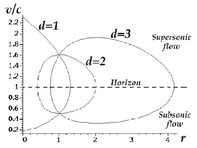
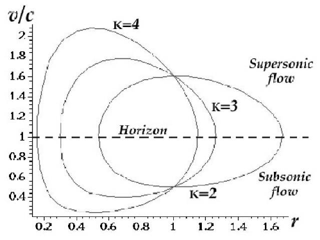
The four things to emphasize here are that:

1. Velocities equal to the speed of sound are indeed attained;

2. The gradient ${\mathrm{d}}v/{\mathrm{d}}r$ is indeed infinite at the acoustic horizon;

3. These particular solutions break down at the acoustic horizon and cannot be extended beyond it;

4. The particular solutions which we have obtained all exhibit a double-valued behaviour, there is a branch with subsonic flow that speeds up and reaches $v=c$ at the acoustic horizon; and there is a second supersonic branch, defined on the same spatial region, that slows down and reaches $v=c$ at the acoustic horizon. Mathematically, this happens because the equation $x=\ln x+k$, with $k$ a constant, has two solutions when $k<1$.

If there is no external body force ($\mbox{\sc k}=0$), then $d=1$ is uninteresting (the velocity is constant). If we now look at $d=2$ and higher then equation (3.55) again easily gives us the acceleration of the fluid

$$a=v\;{{\mathrm{d}}v\over{\mathrm{d}}r}=-v^{2}\;{c_{\mathrm{s}}^{2}{(d-1)/r}\over c_{\mathrm{s}}^{2}-v^{2}}\;,$$ (3.73)

Explicit integration leads us to the solution

$$r=r_{0}\;\left(\frac{v}{v_{0}}\right)^{\frac{1}{1-d}}\exp\left(\frac{v^{2}-v^{2}_{0}}{2(d-1)c_{\mathrm{s}}^{2}}\right),$$ (3.74)

which is equivalent to equation (3.66) with $\mbox{\sc k}=0$. This can easily be plotted for different values of the dimension $d$ as shown in figure 3.3.

Figure 3.3: Plot of the solution of equation (3.66) for $\mbox{\sc k}=0$ with the same initial values. ($c=1$, $r_{0}=1$, and $v_{0}=1/2$.) Note the triviality of the $d=1$ solution, which exhibits two branches, with subsonic and supersonic speeds respectively.

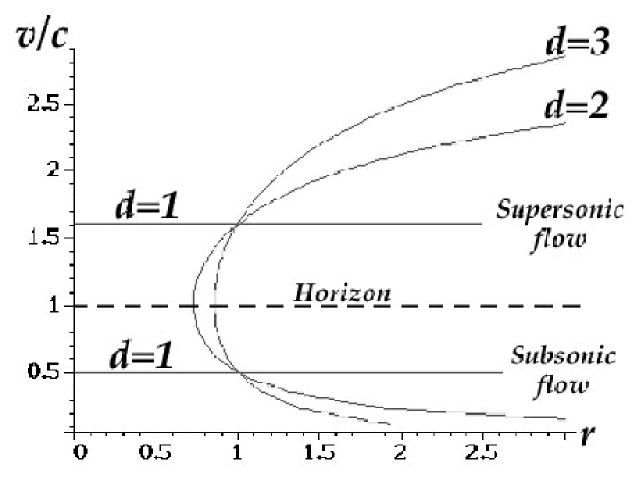
For $\mbox{\sc k}<0$ the solutions are plotted in figure 3.4.

Figure 3.4: Plot of the solution of equation (3.66) for $d=1,2,3$, and $\mbox{\sc k}=-c_{\mathrm{s}}^{2}/r_{0}$, where we again set $c=1$, $r_{0}=1$, and $v_{0}=1/2$.

Finally it is interesting to compare the different behaviour of the solutions for the different signs of the body force as shown in figure 3.5.

In all three cases ($\mbox{\sc k}>0$, $\mbox{\sc k}=0$, $\mbox{\sc k}<0$) we see that the acoustic horizon does in fact form as naively expected, and that the surface gravity and acceleration are indeed infinite at the acoustic horizon. Naturally, this should be viewed as evidence that some of the technical assumptions usually made are no longer valid as the horizon is approached. In particular in the next section (section 3.4.3) we shall discuss the role of viscosity as a regulator for keeping the surface gravity finite.

Figure 3.5: Plot of the solutions of equation (3.66) for $\mbox{\sc k}=\pm 1,0$ and $d=2$, with $c=1$, $r_{0}=1$, and $v_{0}=1/2$.

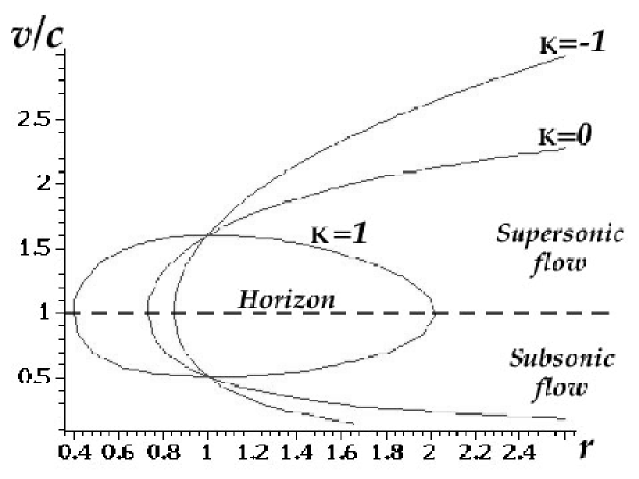
Schwarzschild geometry

So far, the discussion has concerned the attainability of acoustic horizons in general, without focusing on any particular acoustic geometry. A more specific, and rather attractive possibility is to attempt to build a flow with an acoustic metric that is as close as possible to one of the standard black hole metrics of general relativity. We have seen in section 3.2.2 that this is actually conceivable and that the acoustic line element which one obtains is conformal to the Painlevé–Gullstrand form of the Schwarzschild geometry.

This possibility has stimulated considerable work concerning the physical realization of an experimental setup that could actually produce such a flow (or, more precisely, a two-dimensional version of it [207]).

We have seen that for this kind of fluid configuration the potential must be carefully chosen to be of the form given in Eq. (3.32), which will not be easy to do in a laboratory. If one does manage to construct such a potential $\Phi(r)$ it will automatically fulfill the fine-tuning condition (3.48) at the acoustic horizon, $r_{\mathrm{h}}=2M/c_{\mathrm{s}}^{2}$. This is only to be expected, because ${\mathrm{d}}v/{\mathrm{d}}r=-\sqrt{G_{\mathrm{N}}M/2r^{3}}$ diverges only as $r\to 0$. Also, since we know that the surface gravity of a Schwarzschild black hole is finite, any fluid flow that reproduces the Schwarzschild geometry must by definition satisfy the fine tuning condition for a finite surface gravity.

Figure 3.6: Plot of the solutions of equation (3.66) for the potential (3.32), with $G_{\mathrm{N}}M=1/2$, $d=3$, $c=1$, and $r_{0}=4$. The corresponding boundary conditions are $v_{0}=0.4$, $v_{0}=0.5$, and $v_{0}=0.6$.

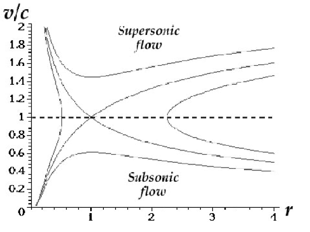
Looking at the issue from the point of view discussed at the end of section 3.4.1, one expects that, given the potential (3.32), the value $v_{0}=\sqrt{2G_{\mathrm{N}}M/r_{0}}$ is the solution of equations (3.68) and (3.69), while $v(r)=\sqrt{2G_{\mathrm{N}}M/r}$ is the corresponding eigenfunction that is selected by the requirement of having a regular flow. This is indeed the case: Equation (3.68) now gives $r_{\mathrm{h}}=2G_{\mathrm{N}}M/c_{\mathrm{s}}^{2}$ which, when substituted into (3.69), leads to the following equation for $v_{0}$:

$${c_{\mathrm{s}}^{2}\over 2}\,\ln\left({2G_{\mathrm{N}}M\over r_{0}v_{0}^{2}}\right)+{v_{0}^{2}\over 2}={G_{\mathrm{N}}M\over r_{0}}.$$ (3.75)

It is trivial to check that $v_{0}=\sqrt{2G_{\mathrm{N}}M/r_{0}}$ is, in fact, a solution of (3.75).

Considering the same potential (3.32), but values of $v_{0}$ different from $\sqrt{2G_{\mathrm{N}}M/r_{0}}$, corresponds to flows either with no horizon, or in which $({\mathrm{d}}v/{\mathrm{d}}r)_{\mathrm{h}}$ diverges. This is evident in figure 3.6, which confirms the “eigenvalue character” of the problem of finding a regular flow. Notice that there are two solutions that are regular at the horizon, with opposite values of $({\mathrm{d}}v/{\mathrm{d}}r)_{\mathrm{h}}$, in full agreement with the fact that equation (3.64) only determines the square of $({\mathrm{d}}v/{\mathrm{d}}r)_{\mathrm{h}}$.

3.4.3 Viscosity

Coming back to the issue of the stability of the acoustic horizon for constant body force (the easiest sort of potential to set up experimentally), one can ask if there are alternatives to the breakdown of stationarity of the flow in order to avoid the divergence of the gradients of physical quantities at the horizon. We shall now see that a general, alternative, way for the fluid to avoid these divergences is to develop a viscosity component at the onset of acoustic horizons. This way not only tames the divergences but can in principle provide the mechanism for the mode regeneration that would allow the presence of the Hawking radiation.

General equations for viscid flow

In the presence of viscosity, the general situation is governed by the Navier–Stokes equation (3.7), from which we deduce (again confining attention to stationary spherical symmetry)

$$a=v\;{{\mathrm{d}}v\over{\mathrm{d}}r}=-{v^{2}\over c_{\mathrm{s}}^{2}-v^{2}}\;\left[\frac{c_{\mathrm{s}}^{2}(d-1)}{r}-\frac{{\mathrm{d}}\Phi}{{\mathrm{d}}r}+\bar{\nu}\left(\frac{{\mathrm{d}}^{2}v}{{\mathrm{d}}r^{2}}+\frac{(d-1)}{r}{{\mathrm{d}}v\over{\mathrm{d}}r}-\frac{(d-1)v}{r^{2}}\right)\right]$$ (3.76)

Here we have rescaled the viscosity coefficient in such a way that $\bar{\nu}={4\over 3}\nu$.

The acceleration is then infinite at the horizon unless

$$\left(1-\frac{\bar{\nu}}{c_{\mathrm{s}}r_{\rm h}}\right){c_{\mathrm{s}}^{2}(d-1)\over r_{\mathrm{h}}}-\left.{{\mathrm{d}}\Phi\over{\mathrm{d}}r}\right|_{\mathrm{h}}+\bar{\nu}\left[{{\mathrm{d}}^{2}v\over dr^{2}}+\frac{(d-1)}{r_{\rm h}}{{\mathrm{d}}v\over{\mathrm{d}}r}\right]_{\mathrm{h}}=0.$$ (3.77)

Since this involves higher-order derivatives at the horizon, it can no longer be regarded as a fine-tuning constraint, or as an equation for $r_{\mathrm{h}}$, but merely as a statement about the shape of the velocity profile near the horizon.

Although it is possible to find the general solutions for $v$ and ${\mathrm{d}}v/{\mathrm{d}}r$ [13], it is unfortunately impractical to find an analytic form for ${\mathrm{d}}^{2}v/{\mathrm{d}}r^{2}$ and hence we must resort to the numerical analysis of special cases.

$d=1$, constant body force

Even the case of constant body force is intractable unless $d=1$, in which case we get (following the steps above)

$$a=v\;{{\mathrm{d}}v\over{\mathrm{d}}r}=-v^{2}\;{-\mbox{\sc k}+\bar{\nu}({{\mathrm{d}}^{2}v/{\mathrm{d}}r^{2}})\over c_{\mathrm{s}}^{2}-v^{2}}.$$ (3.78)

That is

$${{\mathrm{d}}v\over{\mathrm{d}}r}=-v\;{-\mbox{\sc k}+\bar{\nu}({{\mathrm{d}}^{2}v/{\mathrm{d}}r^{2}})\over c_{\mathrm{s}}^{2}-v^{2}}.$$ (3.79)

This single second-order differential equation can be turned into an autonomous system of first-order equations

$$\left\{\begin{array}[]{lll}\displaystyle{\frac{{\mathrm{d}}v}{{\mathrm{d}}r}}&=&\Pi,\\ &&\\ \displaystyle{\frac{{\mathrm{d}}\Pi}{{\mathrm{d}}r}}&=&\displaystyle{\frac{\mbox{\sc k}}{\bar{\nu}}+\frac{v}{\bar{\nu}}\left(1-\frac{c_{\mathrm{s}}^{2}}{v^{2}}\right)\Pi}.\end{array}\right.$$ (3.80)

We can plot the flow of this autonomous system in the usual way and it clearly shows that it is possible to cross the acoustic horizon $v=c$ at arbitrary accelerations $a_{\mathrm{h}}$ and arbitrary surface gravity $g_{\mathrm{h}}$ (see figure 3.7).

Figure 3.7: Plot of the phase space for $d=1$, $\mbox{\sc k}=\mbox{constant}>0$, and nonzero viscosity. The transverse line identifies a separatrix in the integral curves. Note that the integral curves can intersect the acoustic horizon at arbitrary values of the surface gravity.

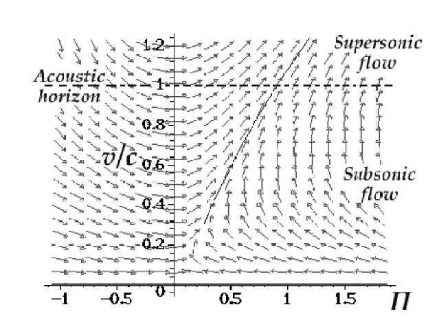
$d=1$, zero body force

If $d=1$ and $\mbox{\sc k}=0$ the once-integrated equation for ${\mathrm{d}}v(r)/{\mathrm{d}}r$ reduces to

$$\left.{{\mathrm{d}}v\over{\mathrm{d}}r}\right|_{r}=\left.{{\mathrm{d}}v\over{\mathrm{d}}r}\right|_{r_{0}}-{1\over 2\bar{\nu}}\;\left[c_{\mathrm{s}}^{2}\;\ln\left(\frac{v^{2}}{v^{2}_{0}}\right)-v^{2}+v^{2}_{0}\right].$$ (3.81)

In this particular case the analysis is sufficiently simple that we can say something about the acceleration at the horizon, namely

$$\left.{{\mathrm{d}}v\over{\mathrm{d}}r}\right|_{\mathrm{h}}=\left.{{\mathrm{d}}v\over{\mathrm{d}}r}\right|_{r_{0}}-{1\over 2\bar{\nu}}\;\left[c_{\mathrm{s}}^{2}\;\ln\left(\frac{c_{\mathrm{s}}^{2}}{v^{2}_{0}}\right)-c_{\mathrm{s}}^{2}+v^{2}_{0}\right].$$ (3.82)

That is

$$g_{\mathrm{h}}=a_{\mathrm{h}}=c_{\mathrm{s}}\left.{{\mathrm{d}}v\over{\mathrm{d}}r}\right|_{r_{0}}-{c_{\mathrm{s}}\over 2\bar{\nu}}\;\left[c_{\mathrm{s}}^{2}\;\ln\left(\frac{c_{\mathrm{s}}^{2}}{v^{2}_{0}}\right)-c_{\mathrm{s}}^{2}+v^{2}_{0}\right].$$ (3.83)

This is an explicit analytic verification that viscosity regularizes the surface gravity of the acoustic horizon.

We can plot the flow in the usual way and it again clearly shows that it is possible to cross the acoustic horizon $v=c$ at arbitrary accelerations $a_{\mathrm{h}}$ (see figure 3.8).

Figure 3.8: Plot of the phase space for $d=1$, $\mbox{\sc k}=0$, and nonzero viscosity. Again note that the integral curves can intersect the acoustic horizon at arbitrary values of the surface gravity.

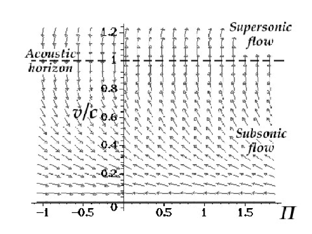
$d>1$, constant body force

For the case of $d>1$ an analytic solution cannot be found even for constant body force. The relevant equation is The relevant equation is

$${{\mathrm{d}}^{2}v\over{\mathrm{d}}r^{2}}+\left({(d-1)\over r}+{1\over\bar{\nu}}{c^{2}-v^{2}\over v}\right){{\mathrm{d}}v\over{\mathrm{d}}r}-{(d-1)v\over r^{2}}={1\over\bar{\nu}}\left(\mbox{\sc k}-{c^{2}(d-1)\over r}\right),$$ (3.84)

which can be recast as

$$\left\{\begin{array}[]{lll}\displaystyle{{{\mathrm{d}}v\over{\mathrm{d}}r}}&=&\Pi\\ &&\\ \displaystyle{\frac{{\mathrm{d}}\Pi}{{\mathrm{d}}r}}&=&{\displaystyle{1\over\bar{\nu}}\left(\mbox{\sc k}-\frac{c^{2}(d-1)}{r}\right)+{(d-1)v\over r^{2}}+\left(\frac{v}{\bar{\nu}}\left(1-\frac{c^{2}}{v^{2}}\right)-{(d-1)\over r}\right)\Pi}.\end{array}\right.$$ (3.85)

This is no longer an autonomous system of differential equations, (there is now an explicit $r$ dependence) and so a flow diagram is meaningless. Nonetheless the system can be treated numerically and curves plotted as a function of initial conditions. As an example we plot some curves in the phase space for $d=2$, and verify that at least some of these curves imply formation of an acoustic horizon.

Figure 3.9: Plot of some solutions of the non-autonomous system (3.85) for various initial conditions for $d=2$, $\mbox{\sc k}=\mbox{constant}$, and nonzero viscosity. Note that at least some of these curves intersect the acoustic horizon, and do so at various finite values of the surface gravity.

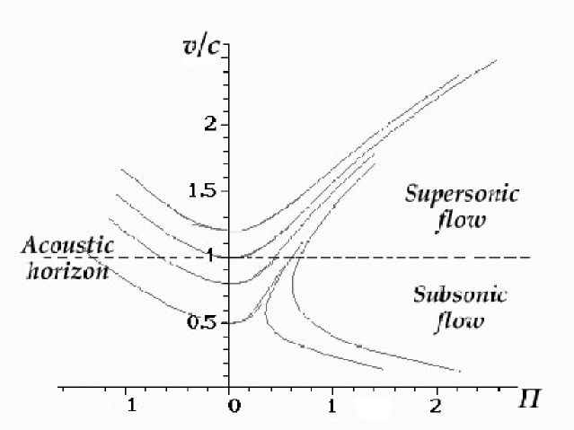
As a final remark it can be useful to discuss briefly the effect of viscosity in relation to the Hawking radiation. It has been shown that the addition of viscosity to the fluid-dynamical equations is equivalent to the introduction of an explicit violation of Lorentz invariance at short scales [185]. In this case one may wonder whether such an explicit breakdown would not lead to a suppression of the Hawking flux as well. In fact the violation of Lorentz invariance is important for wavelengths of order $k\approx k_{0}\approx c_{\mathrm{s}}/\bar{\nu}$ [185], introducing in this way a sort of cutoff (via a modified dispersion relation) for short wavelengths which, as we have discussed, can dramatically affect the Hawking flux. In this case the same factor which removes the unphysical divergences at the acoustic horizons would also “kill” the phenomenon which we are looking for.

This problem has been extensively discussed in the literature (see e.g. [193]) and it can be shown that such a violation of Lorentz invariance is not only harmless but even natural. In particular the viscosity can be shown to induce [185] those sorts of modification of the phonon dispersion relation which are actually required for circumventing the problem cited above [181, 182, 184, 193].

The emergence of viscosity appears then to be indeed a crucial factor for allowing the formation of acoustic horizons and, at the same time, for implementing the mechanism of “mode regeneration” which should permit Hawking radiation in the presence of a short-distance cutoff.

3.4.4 Discussion

Let us summarize the results that we have obtained for a fluid subjected to a given external potential. In the viscosity-free, stationary case, we have seen that if the flow possesses an acoustic horizon, the gradients of physical quantities, as well as the surface gravity and the corresponding Hawking flux, in general exhibit formal divergences. There are two ways in which a real fluid can circumvent this physically unpalatable result. For a broad class of potentials, there is one particular flow which is regular everywhere, even at the horizon. In this case, it is obvious that the fluid itself will “choose” such a configuration. Mathematically, imposing a regularity condition at the horizon amounts to formulating an eigenvalue problem. Unfortunately, there are physically interesting potentials — such as a linear one — for which this is impossible. In such cases, the divergences will be avoided in reality simply because one or both of the simplifying hypothesis (stationarity, no viscosity), become invalid as $v\to c$.

In conclusion, we view the analytic and numerical results obtained in this section as both a danger and an opportunity. They are a danger because infinite accelerations are clearly unphysical and indicate that the idealization of considering an irrotational barotropic inviscid perfect fluid (and this idealization underlies the standard derivations of the notion of the acoustic metric [180, 183, 185]), is sure to break down in the neighborhood of any putative acoustic horizon.

On the other hand, this may be viewed as an opportunity: once we regulate the infinite surface gravity, by adding for instance a finite viscosity, we find that the surface gravity becomes an extra free parameter, divorced from naive estimates based on the geometry of the fluid flow (3.39). This suggests that detecting the acoustic Hawking effect could be much easier than expected once one manages to actually form an acoustic horizon.

3.5 Prospects: condensed matter black holes?

We will end this chapter by discussing a recent development in the study of possible laboratory realizations of event horizons. The basic point which makes conceivable their formation in hydrodynamics is that fluid perturbations in their propagation experience a Lorentzian structure which has a “limit” velocity equal to the sound speed $c_{\mathrm{s}}$. Since a fluid can in principle flow at supersonic speeds (such as, for example, in the case of shock waves) then it is possible to conceive the formation of horizons for phonons.

Another possibility that one can be tempted to explore is to instead work in a regime where light itself is “slowed down” to such an extent that a fluid flow can be faster than the light velocity. This slowing down of light is now a concrete reality: in fact, more and more refined techniques now exist to allow us to make the refractive index of some materials extremely large. Experimental physicists have now managed to get refractive indices up to $n\approx 10^{7}$ giving a light speed of order $v=c/n\approx 10$meters/second [210]. This makes the proposal to build optical hydrodynamical black holes extremely appealing.

Recently Leonhardt and Piwnicki [211, 212, 213] have proposed a model of a dielectric fluid where the propagation of electromagnetic waves is described by an effective metric which is actually an algebraic combination of the refractive index, the fluid velocity and the background Minkowski metric . In particular, in the case of non-dispersive media light experiences a metric of the form [211]:

$$g_{\mu\nu}(t,{\mathbf{x}})\equiv\left[\matrix{(\frac{1}{n^{2}}-\frac{{\rm u}^{2}}{c^{2}})&\vdots&+{{\rm u}\over c}^{j}\cr\cdots\cdots\cdots\cdots&\cdot&\cdots\cdots\cr+{{\rm u}\over c}^{i}&\vdots&-\delta_{ij}\cr}\right].$$ (3.86)

Here $c$ is the speed of light in vacuum and the above form is valid in the limit of large refractive index $n$ and low local velocities ${\mathbf{u}}$ (with respect to $c$) of the medium.

The analogy of this electromagnetic metric with the acoustic metric given in Eq. (3.20) is quite a strict one. It is then easy to see that most of the structures discussed in acoustic geometry can have a correspondence in the case of dielectric flows. In the same way, all of the differences between acoustic manifolds and General Relativity similarly apply in this case.

The most important point is that it is conceivable [215] to build up fluid flows with nozzle or vortex geometries which accelerate a low-compressibility dielectric fluid to velocities which somewhere have radial components faster that the phase velocity of light. Once an “optical event horizon” is built up then a photon Hawking flux should be expected. This will have a near-thermal distribution characterized by a Hawking temperature proportional to the acceleration of the fluid as it crosses the horizon. Unfortunately the large values of the refractive index mentioned above have so far been obtained for very dispersive media ($n(\omega)$ has a resonance for some special frequencies). The analogy between these optical black holes and the acoustic ones is not so strict and so no easy exportation of the results can be made.

Finally one can wonder whether some analogue of the easily set up supersonic cavitation configuration which we saw before can be found in the promising case of a dielectric fluid. This introduces us to our discussion in the next chapter where we shall develop a model based on the dynamics of the refractive index for explaining the radiation observed in Sonoluminescence which we mentioned before.

Our approach to Sonoluminescence will make use of spatio-temporal changes in refractive index induced by the fluid dynamics. Though there are some weak formal similarities with the phonon Hawking radiation of this current chapter, it must be emphasised that the basic physics is rather different.

Chapter 4 Toward experimental semiclassical gravity: Sonoluminescence

Chi disputa allegando l’autorità non adopra lo ’ngenio,

ma più tosto la memoria.

Leonardo da Vinci

A belief is like a guillotine,

just as heavy, just as light.

Franz Kafka

In this chapter we shall pursue our study of the possible experimental tests of the dynamical Casimir effect. In particular we shall focus our attention on the phenomenon of Sonoluminescence. We shall develop an original model for explaining the origin of the radiation emitted in this process, based on dynamical particle production from the quantum vacuum driven by a time varying refractive index (which acts as an external field perturbing the QED vacuum). Although the model developed could be greatly improved if further information about the realistic dynamics of the refractive index could be gained from condensed matter studies, it has to be stressed that it is already able to propose some tests amenable to observations.

The contents of this chapter are original and represent an extract from a “corpus” of works [14, 15, 16, 17, 18, 19] dedicated to the subject. All of these have been done in collaboration with Francesco Belgiorno, Matt Visser and Dennis Sciama without the enthusiasm and guidance of whom they would never have appeared.

4.1 Sonoluminescence as a dynamical Casimir Effect

Sonoluminescence (SL) is the phenomenon of light emission by a sound-driven gas bubble in a fluid [216]. In SL experiments, the intensity of a standing sound wave is increased until the pulsations of a bubble of gas trapped at a velocity node have sufficient amplitude to emit brief flashes of light having a “quasi-thermal” spectrum with a “temperature” of several tens of thousands of Kelvin. The basic mechanism of light production in this phenomenon is still highly controversial. We first present a brief summary of the main experimental data (as currently understood) and of their sensitivities to external and internal conditions. For a more detailed discussion see [216].

SL experiments usually deal with bubbles of air in water, with ambient radius $R_{\mathrm{ambient}}\approx 4.5\;\mu{\rm m}$. The bubble is driven by a sound wave of frequency of 20–30 kHz. (Audible frequencies can also be used, at the cost of inducing deafness in the experimental staff.) During the expansion phase, the bubble radius reaches a maximum of order $R_{\mathrm{max}}\approx\;45\;\mu{\rm m}$, followed by a rapid collapse down to a minimum radius of order $R_{\mathrm{min}}\approx 0.5\;\mu{\rm m}$.

Figure 4.1: Typical variation of the bubble radius as a function of time and in relation to the sound wave cycle (dotted line). Note the peculiar oscillatory behaviour after the collapse. The picture is taken from ref. [216].

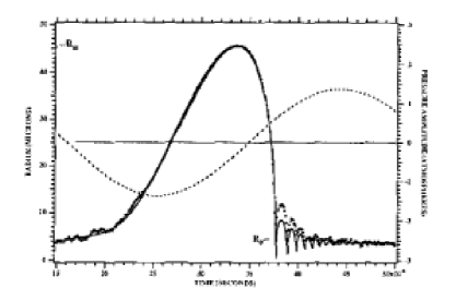
The photons emitted by such a pulsating bubble have typical wavelengths of the order of visible light. The minimum observed wavelengths range between $200\;{\rm nm}$ and $100\;{\rm nm}$. This light appears distributed with a broad-band spectrum (no resonance lines, roughly a power-law spectrum with exponent depending on the gas admixture entrained in the bubble, and with a cutoff in the extreme ultraviolet). For a typical example, see figures 4.2 and 4.3. If one fits the data to a Planck black-body spectrum, the corresponding temperature is several tens of thousands of Kelvin (typically $70,000\;{\rm K}$, though estimates varying from $40,000\;{\rm K}$ to $100,000\;{\rm K}$ are common). There is considerable doubt as to whether or not this temperature parameter corresponds to any real physical temperature. There are about one million photons emitted per flash, and the time-averaged total power emitted is between $30$ and $100\;\hbox{ mW}$.

Figure 4.2: Typical experimental spectrum: The data has been taken from figure 51 of reference 1, and has here been plotted with intensity (in arbitrary units) given as a function of wavelength. Note that no data has been taken at frequencies below the visible range. The spectrum is a broad-band spectrum without significant structure. The physical nature of the cutoff (which occurs in the far ultraviolet) is one of the key issues under debate.

Figure 4.3: Typical experimental spectrum: The data has been taken from figure 51 of reference 1, and has here been plotted with the number spectrum given as a function of frequency.

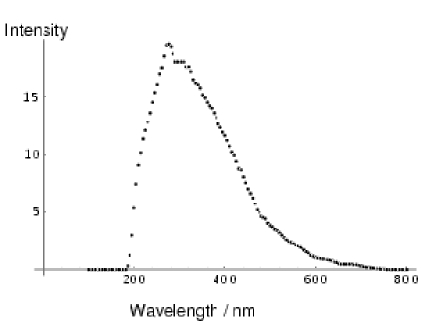
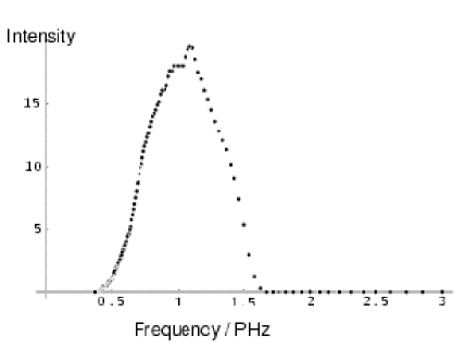
The photons appear to be emitted from a very small spatio-temporal region: Estimated flash widths vary from less than $35\;{\rm ps}$ to more than $380\;{\rm ps}$ depending on the gas entrained in the bubble [217, 218]. There are model-dependent (and controversial) claims that the emission times and flash widths do not depend on wavelength [218]. As for the spatial scale, there are various model-dependent estimates but no direct measurement is available [218]. Although it is clear that there is a frequency cutoff at about $1\;{\rm PHz}$, the physics leading to this is controversial. Standard explanations are

1. a thermal cutoff (deprecated because the observed cutoff is much sharper than exponential) , or

2. the opacity of water in the UV (deprecated because of the observed absence of dissociation effects). Alternatively, Schwinger suggested that the critical issue is that the real part of the refractive index of water goes to unity in the UV (so that there is no change in the Casimir energy during bubble collapse). We shall add another possible contribution to the mix:

3. a rapidly changing refractive index causes photon production with an “adiabatic cutoff’ that depends on the timescale over which the refractive index changes. (Because the observed falloff above the physical cutoff is super-exponential it is clear that this adiabatic effect is at most part of the complete picture.)

Any truly successful theory of SL must also explain a whole series of characteristic sensitivities to different external and internal conditions. Among these dependencies the main one is certainly the mysterious catalytic role of a noble gas admixture. (Most often, this amounts to a few percent in the air entrained in the bubble. One can obtain SL from air bubbles with a $1\%$ content of argon, and also from pure noble gas bubbles, but the phenomenon is practically absent in pure oxygen bubbles.) In fact, it has been suggested that physical processes concentrate the noble gases inside the bubble to the extent that the bubble consists of almost pure noble gas [219], and some experimental results seem to corroborate this suggestion [220].

Other external conditions that influence SL are:

• Magnetic Fields — If the frequency of the driving sound wave is kept fixed, SL disappears above a pressure-dependent threshold magnetic field: $H\geq H_{0}(p)$. On the other hand, for a fixed value of the magnetic field $H_{0}$, there are both upper and lower bounds on the applied pressure that bracket the region of SL, and these bounds are increasing functions of the applied magnetic field [221]. This is often interpreted as suggesting that the primary effect of magnetic fields is to alter the condition for stable bubble oscillations. See. also [222].

• Temperature of the water — If $T_{H_{2}O}$ decreases then the emitted power $W$ increases. The position of the peak of the spectrum depends on $T_{H_{2}O}$. It has been suggested that the increased light emission at lower water temperature is associated with an increased stability of the bubble, allowing for higher driving pressures [223].

These are only the most salient features of the SL phenomenon. In attempting to explain such detailed and specific behaviour the dynamical Casimir approach (QED vacuum approach) encounters problems which are equivalent to those in all of the other approaches. Nevertheless we shall argue that SL explanations using a Casimir-like framework are viable, and merit further investigation.

4.1.1 Casimir models: Schwinger’s approach

The idea of a “Casimir route” to SL is due to Schwinger who several years ago wrote a series of papers [224, 225, 226, 227, 228, 229, 230] regarding the so-called dynamical Casimir effect. Considerable confusion has been caused by Schwinger’s choice of the phrase “dynamical Casimir effect” to describe his particular model. In fact, Schwinger’s original model is not dynamical but is instead quasi-static as the heart of the model lies in comparing two static Casimir energy calculations: one for an expanded bubble and the other for a collapsed bubble. One key issue in Schwinger’s model is thus simply that of calculating Casimir energies for dielectric spheres — and there is already considerable disagreement on this issue. A second and in some ways more critical question is the extent to which this difference in Casimir energies may be converted into real photons during the collapse of the bubble. The original quasi-static incarnation of the Schwinger model had no real way of estimating either photon production efficiency or timing information (when does the flash occur?). In contrast, the model of Eberlein [231, 232, 233] (more fully discussed below) is truly dynamical but uses a much more specific physical approximation — the adiabatic approximation. The two models should not be confused. We shall argue that the observed features of SL force one to make the sudden approximation. We can then estimate the spectrum of the emitted photons by calculating an appropriate Bogoliubov coefficient relating two states of the QED vacuum. The resulting variant of the Schwinger model for SL is then rather tightly constrained, and should be amenable to experimental verification (or falsification) in the near future.

In his papers on SL, Schwinger showed that the dominant bulk contribution to the Casimir energy of a bubble (of dielectric constant $\epsilon_{\mathrm{inside}}$) in a dielectric background (of dielectric constant $\epsilon_{\mathrm{outside}}$) is [227]

$$E_{\mathrm{cavity}} = +2\frac{4\pi}{3}R^{3}\;\int_{0}^{K}{4\pi k^{2}{\mathrm{d}}k\over(2\pi)^{3}}\;\frac{1}{2}\hbar ck\left({1\over\sqrt{\epsilon_{\mathrm{inside}}}}-{1\over\sqrt{\epsilon_{\mathrm{outside}}}}\right)+\cdots$$ (4.1)

$$= +\frac{1}{6\pi}\hbar cR^{3}K^{4}\left({1\over\sqrt{\epsilon_{\mathrm{inside}}}}-{1\over\sqrt{\epsilon_{\mathrm{outside}}}}\right)+\cdots$$

The corresponding number of emitted photons is

$$N = +2\frac{4\pi}{3}R^{3}\;\int_{0}^{K}{4\pi k^{2}{\mathrm{d}}k\over(2\pi)^{3}}\;\frac{1}{2}\left(\frac{\sqrt{\epsilon_{\mathrm{outside}}}}{\sqrt{\epsilon_{\mathrm{inside}}}}-1\right)+\cdots$$ (4.2)

$$= +\frac{2}{9\pi}(RK)^{3}\left(\frac{\sqrt{\epsilon_{\mathrm{outside}}}}{\sqrt{\epsilon_{\mathrm{inside}}}}-1\right)+\cdots$$

Here we have inserted an explicit factor of two with respect to Schwinger’s papers to take into account both photon polarizations. There are additional sub-dominant finite volume effects discussed in [234, 235, 236]. Schwinger’s result can also be rephrased in a clearer and more general form as [234, 235, 236]:

$$E_{\mathrm{cavity}}=+2V\int_{0}^{K}\frac{{\mathrm{d}}^{3}\vec{k}}{(2\pi)^{3}}\;\frac{1}{2}\hbar\left[\omega_{\mathrm{inside}}(k)-\omega_{\mathrm{outside}}(k)\right]+\cdots$$ (4.3)

$$N=+2V\int_{0}^{K}\frac{{\mathrm{d}}^{3}\vec{k}}{(2\pi)^{3}}\;\frac{1}{2}\left[{\omega_{\mathrm{inside}}(k)\over\omega_{\mathrm{outside}}(k)}-1\right]+\cdots$$ (4.4)

Here it is evident that the Casimir energy can be interpreted as a difference in zero point energies due to the different dispersion relations inside and outside the bubble. The quantity $K$ appearing above is a high-wavenumber cutoff that characterizes the wavenumber at which the (real part of) the refractive indices ($n=\sqrt{\epsilon}$) drop to their vacuum values. It is important to stress that this cutoff it is not a regularization artifact to be removed at the end of the calculation. The cutoff has a true physical meaning in its own right.

The two main points of strength of models based on zero point fluctuations (e.g., Schwinger’s model and its variants) are:

1. There is no actual production of far ultraviolet photons (because the refractive index goes to unity in the far ultraviolet) and so one does not expect the dissociation effects in water that other models imply. Models based on the quantum vacuum automatically provide a cutoff in the far ultraviolet because of the behaviour of the refractive index — this observation goes back to Schwinger’s first papers on the subject.

2. One naturally gets the right energy budget. For $n_{\mathrm{outside}}\approx 1.3$, $n_{\mathrm{inside}}\approx 1$, $K$ in the ultra-violet, and $R\approx R_{\mathrm{max}}$, the change in the static Casimir energy is approximately equal to the energy emitted during each cycle.

This last issue has been the subject of a heated debate. Milton and collaborators [237, 238, 239, 240], Brevik et al [241] and Nesterenko and Pirozhenko [242], have strongly criticized Schwinger’s result claiming that actually the Casimir energy contains at best a surface term, the bulk term being discarded via (in our opinion) a physically dubious renormalization argument. These points have been discussed extensively in [234, 235, 236] where it is emphasized that one has to compare two different physical configurations of the same system, corresponding to two different geometrical configurations of matter, and thus must compare two different quantum states defined on the same spacetime. In a situation like Schwinger’s model for SL one has to subtract from the zero point energy (ZPE) for a vacuum bubble in water the ZPE for water filling all space. It is clear that in this case the bulk term is physical and must be taken into account. Surface terms are also present, and eventually other higher order correction terms, but they prove not to be dominant for sufficiently large cavities [236].

While the contentious issues of how to define the Casimir energy are successfully dealt with in [234, 235, 236], one of the subsidiary aims of the research which we shall present here has been to side-step this whole argument and provide an independent calculation demonstrating efficient photon production. After the former works I think that the issue is now completely fixed and Schwinger’s correctness vindicated.

In contrast to the points of strength outlined above, the main weakness of the original quasi-static version of Schwinger’s idea is that there is no real way to calculate either timing information or conversion efficiency. A naive estimate is to simply and directly link power produced to the change in volume of the bubble. As pointed out by Barber et al. [216], this assumption would imply that the main production of photons may be expected when the fractional rate of change of the volume is a maximum, which is experimentally found to occur near to the maximum radius. However, the emission of light is experimentally found to occur near the point of minimum radius, where the rate of change of area is maximum. Everything else being equal, this would seem to indicate a surface dependence and might be interpreted as a true weakness of the dynamical Casimir explanation of SL. In fact we shall show that the situation is considerably more complex than might naively be thought, but before this we shall discuss the other main Casimir model for Sonoluminescence.

4.1.2 Eberlein’s dynamical model for SL

The quantum vacuum approach to SL was developed extensively in the work of Eberlein [231, 232, 233]. The basic mechanism in Eberlein’s approach is a particular implementation of the dynamical Casimir effect: Photons are assumed to be produced due to an adiabatic change of the refractive index in the region of space between the minimum and the maximum bubble radius (a related discussion for time-varying but spatially-constant refractive index can be found in the discussion by Yablonovitch [244]). This physical framework is actually implemented via a boundary between two dielectric media which accelerates with respect to the rest frame of the quantum vacuum state. The change in the zero-point modes of the fields produces a non-zero radiation flux. Eberlein’s contribution was to take the general phenomenon of photon generation by moving dielectric boundaries and attempt a specific implementation of these ideas as a candidate for explaining SL.

It is important to realize that this is a second-order effect. Although he was unable to provide a calculation to demonstrate it, Schwinger’s original discussion is posited on the direct conversion of zero point fluctuations in the expanded bubble vacuum state into real photons plus zero point fluctuations in the collapsed bubble vacuum state. Eberlein’s mechanism is a more subtle (and much weaker) effect involving the response of the atoms in the dielectric medium to acceleration through the zero-point fluctuations. The two mechanisms are quite distinct and considerable confusion has been engendered by conflating the two mechanisms. Criticisms of the Eberlein mechanism do not necessarily apply to the Schwinger mechanism, and vice versa.

In the Eberlein analysis the motion of the bubble boundary is taken into account by introducing a velocity-dependent perturbation to the usual Hamiltonian of electromagnetism:

$$H_{\epsilon} \!= \!\frac{1}{2}\int{\rm d}^{3}{\bf r}\left({{\bf D}^{2}\over\epsilon}+{\bf B}^{2}\right)\;,$$ (4.5)

$$\Delta H \!= \!\beta\int{\rm d}^{3}{\bf r}\frac{\epsilon-1}{\epsilon}\;({\bf D}\wedge{\bf B})\cdot{\bf\hat{r}}\;.$$ (4.6)

This is an approximate low-velocity result coming from a power series expansion in the speed of the bubble wall $\beta=\dot{R}/c$. The bubble wall is known to collapse with supersonic velocity, values of Mach 4 are often quoted, but this is still completely non-relativistic with $\beta\approx 10^{-5}$.

The Eberlein calculation consists of a novel mixture of the standard adiabatic approximation with perturbation theory. In principle, the adiabatic approximation requires the knowledge of the complete set of eigenfunctions of the Hamiltonian for any allowed value of the parameter $\beta$. In the present case only the eigenfunctions of part of the Hamiltonian, namely those of $H_{\epsilon}$, are known (and these are known explicitly only in the adiabatic approximation where $\epsilon$ is treated as time-independent.) The calculation consists of initially invoking the standard application of the adiabatic approximation to the full Hamiltonian, then formally calculating the transition coefficients for the vacuum to two photon transition to first order in $\beta$, and finally in explicitly calculating the radiated energy and spectral density. In this last step Eberlein used an approximation valid only in the limit $kR\gg 1$ which means the limit of photon wavelengths much smaller than the bubble radius. This implies that the calculation will completely miss any resonances that are present.

Eberlein’s final result for the energy radiated over one acoustic cycle is:

$${\cal W}=1.16\>\frac{(n^{2}-1)^{2}}{n^{2}}\,\frac{1}{480\pi}\left[{\hbar\over c^{3}}\right]\int_{0}^{T}{\rm d}\tau\;\frac{\partial^{5}R^{2}(\tau)}{\partial\tau^{5}}\,R(\tau)\beta(\tau)\;.$$ (4.7)

Eberlein approximates $n_{\mathrm{inside}}\approx n_{\mathrm{air}}\approx 1$ and sets $n_{\mathrm{outside}}=n_{\mathrm{water}}\to n$. The $1.16$ is the result of an appropriate numerical integration. The precise nature of the semi-analytic approximations made as a prelude to performing the numerical integration are far from clear.

By a double integration by parts, the above formula can be re-cast as

$${\cal W}=1.16\>\frac{(n^{2}-1)^{2}}{n^{2}}\,\frac{1}{960\pi}\left[{\hbar\over c^{4}}\right]\int_{0}^{T}{\rm d}\tau\;\left(\frac{\partial^{3}R^{2}(\tau)}{\partial\tau^{3}}\right)^{2}.$$ (4.8)

Then the energy radiated is also seen to be proportional to

$$\int_{0}^{T}(\dot{R})^{2}(\ddot{R})^{2}+...$$ (4.9)

explicitly showing that the acceleration of the interface ($\ddot{R}$) and the strength of the perturbation ($\dot{R}$) both contribute to the radiated energy.

The main advantage of this model over the original Schwinger model is the ability to provide basic timing information: In this mechanism the massive burst of photons is produced at and near the turn-around at the minimum radius of the bubble. There the velocity rapidly changes sign, from collapse to re-expansion. This means that the acceleration is peaked at this moment, and so are higher derivatives of the velocity. Other main points of strength of the Eberlein model are the same as previously listed for the Schwinger model plus the ability to explicitly show that one does not need to achieve “real” temperatures of thousands of Kelvin inside the bubble.

As discussed in section 1.3.3, quasi-thermal behaviour is generated in quantum vacuum models by the squeezed nature of the two photon states created [232], and the “temperature” parameter is a measure of the squeezing, not a measure of any real physical temperature .

Of course, one should remember that the experimental data merely indicates an approximately power-law spectrum [$N(\omega)\propto\omega^{\alpha}$] with some sort of cutoff in the ultraviolet, and with an exponent that depends on the gases entrained in the bubble; the much-quoted “temperature” of the SL radiation is merely an indication of the scale of this cutoff $K$.

In spite of these points of strength, Eberlein’s model exhibits significant weaknesses:

1. The calculation is based on an adiabatic approximation which does not seem consistent with results. The adiabatic approximation would seem to be justified in the SL case by the fact that the frequency $\Omega$ of the driving sound is of the order of tens of kHz, while that of the emitted light is of the order of $10^{15}$ Hz. But if one takes a timescale for bubble collapse of the order of milliseconds, or even microseconds, then photon production is extremely inefficient, being exponentially suppressed [as we shall soon see] by a factor of $\exp(-\omega/\Omega)$.

   In order to compare with the experimental data, the model requires, as external input, the time dependence of the bubble radius. This is expressed as a function of a parameter $\gamma$ which describes the time scale of the collapse and re-expansion process. In order to be compatible with the experimental values for emitted power $\cal W$ one has to fix $\gamma\approx 10\;{\rm fs}$. This is far too short a time to be compatible with the adiabatic approximation. Although one may claim that the precise numerical value of the timescale can ultimately be modified by the eventual inclusion of resonances it would seem reasonable to take this ten femtosecond figure as a first self-consistent approximation for the characteristic timescale of the driving system (the pulsating bubble). Unfortunately, the characteristic timescale of the collapsing bubble then comes out to be of the same order as the characteristic period of the emitted photons, violating the adiabatic approximation used in deriving the result. Attempts at bootstrapping the calculation into self-consistency instead bring it to a regime where the adiabatic approximation underlying the scheme cannot be trusted.

2. The Eberlein calculation cannot deal with any resonances that may be present. Eberlein does consider resonances to be a possible important correction to her model, but she is considering “classical” resonances (scale of the cavity of the same order as the wavelength of the photons) instead of the probably more interesting possibility of parametric resonances.

Finally one should mention a recent calculation that gives qualitatively the same results as the Eberlein model although leading to different formulae. Schützhold, Plunien, and Soff [245] adopted a slightly different decomposition into unperturbed and perturbing Hamiltonians and their result for the total energy emitted per cycle is given analytically by

$${\cal W}={n^{2}(n^{2}-1)^{2}\over 1890\pi}\left[{\hbar\over c^{6}}\right]\int_{0}^{T}{\rm d}\tau\;\left(\frac{\partial^{4}R^{3}(\tau)}{\partial\tau^{4}}\right)^{2}.$$ (4.10)

The key differences are that this formula is analytic (rather than numerical) and involves fourth derivatives of the volume of the bubble (rather than third derivatives of the surface area). The main reason for the discrepancy between this and Eberlein’s result can be seen as being due to a different choice of the dependence on $r$ of $\beta(r,t)$. In reference [245] they considered the more physical case of a localized disturbance that yields significant contributions only over a bounded volume. (Eberlein makes the simplifying assumption that $\beta(r,t)$ is a function of $t$ only, which is incompatible with continuity and the essentially constant density of water. In contrast, Schützhold et al. take the radial velocity of the water outside the bubble to be $\beta(r,t)=f(t)/r^{2}$.)

Putting these models aside, and before proposing new routes for developing further research in SL, I shall give below a more detailed discussion of some important points of Schwinger’s model which seem to be crucial in order to understand the possibility of a vacuum explanation for SL.

4.1.3 Timescales: The need for a sudden approximation

One of the key features of photon production by a space-dependent and time-dependent refractive index is that for a change occurring on a timescale $\tau$, the amount of photon production is exponentially suppressed by an amount $\exp(-\omega\tau)$.

The importance for SL is that the experimental spectrum is not  exponentially suppressed at least out to the far ultraviolet. Therefore any mechanism of Casimir-induced photon production based on an adiabatic approximation is destined to failure: Since the exponential suppression is not visible out to $\omega\approx 10^{15}\hbox{ Hz}$, it follows that if  SL is to be attributed to photon production from a time-dependent external field (i.e., to a dynamical Casimir effect), then the timescale for change of this field should be of order a femtosecond.

In the Eberlein model of sonoluminescence the time varying external field is the bubble refractive index. Its variation (consequential to the change in the bubble radius) perturbs the QED vacuum and hence leads to the emission of photons. Unfortunately the bubble radius changes on a much longer time scale than femtoseconds so any Casimir–based model has to take into account that the change in the refractive index cannot be due just to the change in the bubble radius.

The SL flash is known to occur at or shortly after the point of maximum compression. The light flash is emitted when the bubble is at or near minimum radius $R_{\mathrm{min}}\approx 0.5\;\mu\hbox{m}=500\;\hbox{nm}$. Note that to get an order femtosecond change in refractive index over a distance of about $500\;{\rm nm}$, the change in refractive index has to propagate at relativistic speeds. To achieve this, one must adjust basic aspects of the model: We will move away from the original Schwinger suggestion, in that it is no longer the collapse from $R_{\mathrm{max}}$ to $R_{\mathrm{min}}$ that is important. Instead we will postulate a rapid (order femtosecond) change in refractive index of the gas bubble when it hits the van der Waals hard core.

It is important to stress that, once one takes into account the refractive index of the final state, this condition can be somewhat relaxed. We shall ultimately see in section 4.2.3 that we can tolerate a refractive index that changes as slowly as on a picosecond timescale, but this is still far to rapid to be associated with physical collapse of the bubble. For the time being we focus on the femtosecond timescale (which actually makes things more difficult for us) to check the physical plausibility of the scenario, but keep in mind that eventually things can be relaxed by a few orders of magnitude.

The underlying idea is that there is some physical process that gives rise to a sudden change of the refractive index inside the bubble when it reaches maximum compression. We have to ensure that the velocity of mechanical perturbations, that is the sound velocity, can be a significant fraction of the speed of light in this critical regime. Actually this condition can also be slightly relaxed: one can conceive of the change in refractive index being driven by a shock wave that appears at the van der Waals hard core. Now a shock wave is by definition a supersonic phenomenon. If the velocity of sound is itself already extremely high then the shock wave velocity may be even higher.

Most of the viable models for the gas dynamics during the collapse predict the formation of strong shock waves; so we are adapting physics already envisaged in the literature. At the same time we are asking for less extreme conditions (e.g., we can be much more relaxed regarding the focusing of these shock waves) in that we just need a rapid change of the refractive index of the entrained gas, and do not need to propose any overheating to “stellar” temperatures. Noticeably dramatic changes in the refractive index (but that of the surrounding water) due to the huge compression generated by shock waves have already been considered in the literature [246] (cf. page 5437).

4.1.4 Bubble at the van der Waals hard core

In support of this proposal I shall first show that the minimum radius experimentally observed is of the same order as the van der Waals hard core radius $R_{\mathrm{hc}}$. The latter can be deduced as follows: It is known that the van der Waals excluded volume for air is $b=$0.036 l/mol [247]. The minimum possible value of the volume is then $V_{\mathrm{hc}}=b\cdot(\rho V_{\mathrm{ambient}})/m$, where $(\rho V_{\mathrm{ambient}})/m$ gives the number of moles and $V_{\mathrm{ambient}}$ is the ambient value of the volume. From $R_{\mathrm{hc}}=R_{\mathrm{ambient}}\cdot(b\rho/\mu)^{1/3}$ and assuming for the density of air $\rho=10^{-3}\;{\rm gr}/{\rm cm}^{3}$ [$1.3\times 10^{-3}\;{\rm gr}/{\rm cm}^{3}$ at STP (standard temperature and pressure)], one gets $R_{\mathrm{h}c}\sim 0.48\;\mu{\mathrm{m}}$. This value compares favorably with the experimentally observed value of $R_{\mathrm{min}}$. Moreover, the role of the van der Waals hard core in limiting the collapse of the bubble is suggested in [216] (cf. fig. 10, p.78), and a careful hydrodynamic analysis for the case of an Argon bubble [248] reveals that for Sonoluminescence it is necessary that the bubble undergoes a so called strongly collapsing phase where its minimum radius is indeed very near the hard core radius.

It is crucial to realize that a van der Waals gas, when compressed to near its maximum density, has a speed of sound that goes relativistic. To see this, write the (non-relativistic) van der Waals equation of state as

$$p={nkT\over 1-nb}-an^{2}={\rho kT/m\over 1-\rho/\rho_{\mathrm{max}}}-a{\rho^{2}\over m^{2}}.$$ (4.11)

Here $n$ is the number density of molecules; $\rho$ is mass density; $m$ is average molecular weight ($m=28.96\;\hbox{amu/molecule}=28.96\;\hbox{gr/mol}$ for air).

Now consider the (isothermal) speed of sound for a van der Waals gas

$$v_{\mathrm{sound}}^{2}=\left({\partial p\over\partial\rho}\right)_{T}={(kT/m)\over(1-\rho/\rho_{\mathrm{max}})^{2}}-2a{\rho\over m^{2}}.$$ (4.12)

Near maximum density this is

$$v_{\mathrm{sound}}\approx{\sqrt{kT/m}\over(1-\rho/\rho_{\mathrm{max}})},$$ (4.13)

and so it will go relativistic (formally infinite) for densities close enough to maximum density .

It is only for the sake of simplicity that it has been considered the isothermal speed of sound. One does not expect the process of bubble collapse and core bounce to be isothermal. Nevertheless, this calculation is sufficient to demonstrate that in general the sound velocity becomes formally infinite (and it is reasonable that it goes relativistic) at the incompressibility limit (where it hits the van der Waals hard core). This conclusion is not limited to the van der Waals equation of state, and is not limited to isothermal (or even isentropic) sound propagation (see [17] for further details). There is something of a puzzle in the fact that hydrodynamic simulations of bubble collapse do not see these relativistic effects. Notably, the simulations by Moss et al [249] seem to suggest collapse, shock wave production, and re-expansion all without ever running into any van der Waals hard core. The fundamental reason for this is that the model equation of state they choose does not have any hard core for the bubble to bounce off. Instead, there are a number of free parameters in their equation of state which are chosen in such a way as to make their equation of state stiff at intermediate densities, even if their equation of state is by construction always soft at van der Waals hard core densities. If the equation of state is made sufficiently stiff at intermediate densities then a bounce can be forced to occur long before hard core densities are encountered. However, as previously mentioned, the experimental data and hydrodynamic analysis seem to indicate that hard core densities are achieved at maximum bubble compression.

Given all this, the use of a relativistic sound speed is now physically justifiable, and the possibility of femtosecond changes in the refractive index is at least physically plausible (even though we cannot say that femtosecond changes in refractive index are guaranteed).

So our new physical picture is this: The “in state” is a small sphere of gas, radius about 500 nm, with some refractive index $n_{\mathrm{gas}}^{\mathrm{in}}$ embedded in water of refractive index $n_{\mathrm{liquid}}$. There is a sudden femtosecond change in refractive index, essentially at constant radius, so the “out state” is gas with refractive index $n_{\mathrm{gas}}^{\mathrm{out}}$ embedded in water of refractive index $n_{\mathrm{liquid}}\;$. In view of this femtosecond change of refractive index, we would be justified in making the sudden approximation for frequencies less than about a PHz.

4.2 Sonoluminescence as a dynamical Casimir effect: Homogeneous model

As a first approach to the problem of estimating the spectrum and efficiency of photon production we can start by studying in detail the basic mechanism of particle creation and to test the consistency of the Casimir energy proposals previously described. With this aim in mind we shall look at the effect of a changing dielectric constant in a homogeneous medium. At this stage of development, we shall not be concerned with the detailed dynamics of the bubble surface, and confine attention to the bulk effects, deferring consideration of finite-volume effects to the next section.

Let us consider two different asymptotic configurations. An “in” configuration with refractive index $n_{\mathrm{in}}$, and an “out” configuration with a refractive index $n_{\mathrm{out}}$. These two configurations will correspond to two different bases for the quantization of the field. (For the sake of simplicity we take, as Schwinger did, only the electric part of QED, reducing the problem to a scalar electrodynamics). The two bases will be related by Bogoliubov coefficients in the usual way. Once we determine these coefficients we easily get the number of created particles per mode and from this the spectrum. Of course it is evident that such a model cannot be considered a fully complete and satisfactory model for SL. This present calculation must still be viewed as a test calculation in which basic features of the Casimir approach to SL are investigated.

In the original version of the Schwinger model it was usual to simplify calculations by using the fact that the dielectric constant of air is approximately equal 1 at standard temperature and pressure (STP), and then dealing only with the dielectric constant of water ($n_{\mathrm{liquid}}=\sqrt{\epsilon_{\mathrm{outside}}}\approx 1.3$). One should avoid this temptation on the grounds that the sonoluminescent flash is known to occur within $500$ picoseconds of the bubble achieving minimum radius. Under these conditions the gases trapped in the bubble are close to the absolute maximum density implied by the hard core repulsion incorporated into the van der Waals equation of state. Gas densities are approximately one million times atmospheric and conditions are nowhere near STP. For this reason we shall explicitly keep track of both initial and final refractive indices.

I shall now describe a simple analytically tractable model for the conversion of zero point fluctuations (Casimir energy) into real photons. The model describes the effects of a time-dependent refractive index in the infinite volume limit. We shall see that for sudden changes in the refractive index the conversion of zero-point fluctuations is highly efficient, being limited only by phase space, whereas adiabatic changes of the refractive index lead to exponentially suppressed photon production.

4.2.1 Defining the model

Take an infinite homogeneous dielectric with a permittivity $\epsilon(t)$ that depends only on time, not on space. The homogeneous (${\mathrm{d}}F=0$) Maxwell equations are

$$B=\nabla\times A;$$ (4.14)

$$E=-\nabla\phi-{1\over c}{\partial A\over\partial t};$$ (4.15)

while the source-free inhomogeneous ($*{\mathrm{d}}*F=0$) Maxwell equations become

$$\nabla\cdot(\epsilon E)=0;$$ (4.16)

$$\nabla\times{B}=+{1\over c}{\partial\over\partial t}(\epsilon E).$$ (4.17)

Substituting into this last equation

$$\nabla\times\left(\nabla\times A\right)=-{1\over c}{\partial\over\partial t}\left[\epsilon\left(\nabla\phi+{1\over c}{\partial A\over\partial t}\right)\right].$$ (4.18)

Suppose that $\epsilon(t)$ depends on time but not space, then

$$(\nabla(\nabla\cdot A)-\nabla^{2}A)=-\nabla{1\over c}{\partial\over\partial t}(\epsilon\phi)-{1\over c^{2}}{\partial\over\partial t}\epsilon{\partial A\over\partial t}.$$ (4.19)

Now adopt a generalized Lorentz gauge

$$\nabla\cdot A+{1\over c}{\partial\over\partial t}(\epsilon\phi)=0.$$ (4.20)

Then the equations of motion reduce to

$${1\over c^{2}}{\partial\over\partial t}\epsilon{\partial A\over\partial t}=\nabla^{2}A.$$ (4.21)

We now introduce a “pseudo-time” parameter by defining

$${\partial\over\partial\tau}=\epsilon(t){\partial\over\partial t}.$$ (4.22)

That is

$$\tau(t)=\int{{\mathrm{d}}t\over\epsilon(t)}.$$ (4.23)

In terms of this pseudo-time parameter the equation of motion is

$${\partial^{2}\over\partial\tau^{2}}A=c^{2}{\epsilon(\tau)}\nabla^{2}A.$$ (4.24)

Compare this with equation (3.86) of Birrell and Davies [4]. Now pick a convenient profile for the permittivity and permeability as a function of this pseudo-time. (This particular choice of time profile for the refractive index is only to make the problem analytically tractable, with a little more work it is possible to consider generic monotonic changes of refractive index and place bounds on the Bogoliubov coefficients [250].) Let us take

$${\epsilon(\tau)} = a+b\tanh(\tau/\tau_{0})$$ (4.25)

$$= {\textstyle{1\over 2}}(n_{\mathrm{in}}^{2}+n_{\mathrm{out}}^{2})+{\textstyle{1\over 2}}(n_{\mathrm{out}}^{2}-n_{\mathrm{in}}^{2})\;\tanh(\tau/\tau_{0}).$$ (4.26)

Here $\tau_{0}$ represents the typical timescale of the change of the refractive index in terms of the pseudo-time we have just defined. We are interested in computing the number of particles that can be created passing from the “in” state ($t\to-\infty$, that is, $\tau\to-\infty$) to the “out” state ($t\to+\infty$, that is, $\tau\to+\infty$). This means we must determine the Bogoliubov coefficients that relate the “in” and “out” bases of the quantum Hilbert space. Defining the inner product as:

$$(\phi_{1},\phi_{2})={\mathrm{i}}\int_{\Sigma_{\tau}}\phi_{1}^{*}\;{\stackrel{{\scriptstyle\leftrightarrow}}{{\partial}}\over\partial\tau}\;\phi_{2}\>{\mathrm{d}}^{3}x,$$ (4.27)

The Bogoliubov coefficients can now be defined as

$$\alpha_{ij} = -({A_{i}^{\mathrm{out}}},{A_{j}^{\mathrm{in}}}),$$ (4.28)

$$\beta_{ij} = ({A_{i}^{\mathrm{out}}}^{*},{A_{j}^{\mathrm{in}}}).$$ (4.29)

Where ${A_{i}^{\mathrm{in}}}$ and ${A_{j}^{\mathrm{out}}}$ are solutions of the wave equation (4.24) in the remote past and remote future respectively. We shall compute the coefficient $\beta_{ij}$ It is this quantity that is linked to the spectrum of the “out” particles present in the “in” vacuum, and it is this quantity that is related to the total energy emitted. With a few minor changes of notation we can just write down the answers directly from pages 60–62 of Birrell and Davies [4]. Birrell and Davies were interested in the problem of particle production engendered by the expansion of the universe in a cosmological context. Although the physical model is radically different here the mathematical aspects of the analysis carry over with some minor translation in the details. Equations (3.88) of Birrell–Davies become

$$\omega^{\tau}_{\mathrm{in}}=k\sqrt{a-b}=k\sqrt{\epsilon_{\mathrm{in}}}=k\;n_{\mathrm{in}};$$ (4.30)

$$\omega^{\tau}_{\mathrm{out}}=k\sqrt{a+b}=k\sqrt{\epsilon_{\mathrm{out}}}=k\;n_{\mathrm{out}};$$ (4.31)

$$\omega^{\tau}_{\pm}={\textstyle{1\over 2}}\;k\;\left|n_{\mathrm{in}}\pm n_{\mathrm{out}}\right|={\textstyle{1\over 2}}|\omega^{\tau}_{\mathrm{in}}\pm\omega^{\tau}_{\mathrm{out}}|.$$ (4.32)

(Here it should be emphasized that these frequencies are those appropriate to the “pseudo-time” $\tau$.) The Bogoliubov $\alpha$ and $\beta$ coefficients can be easily deduced from Birrell–Davies (3.92)+(3.93)

$$\alpha(\vec{k}_{\mathrm{in}},\vec{k}_{\mathrm{out}}) = \frac{\sqrt{\omega^{\tau}_{\mathrm{out}}\;\omega^{\tau}_{\mathrm{in}}}}{\omega^{\tau}_{+}}\;\;{\Gamma(-{\mathrm{i}}\omega^{\tau}_{\mathrm{in}}\tau_{0})\;\Gamma(-{\mathrm{i}}\omega^{\tau}_{\mathrm{out}}\tau_{0})\over\Gamma(-{\mathrm{i}}\omega^{\tau}_{-}\tau_{0})^{2}}\;\delta^{3}(\vec{k}_{\mathrm{in}}-\vec{k}_{\mathrm{out}})$$ (4.33)

$$\beta(\vec{k}_{\mathrm{in}},\vec{k}_{\mathrm{out}}) = -\frac{\sqrt{\omega^{\tau}_{\mathrm{out}}\;\omega^{\tau}_{\mathrm{in}}}}{\omega^{\tau}_{-}}\;\;{\Gamma(-{\mathrm{i}}\omega^{\tau}_{\mathrm{in}}\tau_{0})\;\Gamma({\mathrm{i}}\omega^{\tau}_{\mathrm{out}}\tau_{0})\over\Gamma({\mathrm{i}}\omega^{\tau}_{-}\tau_{0})^{2}}\;\delta^{3}(\vec{k}_{\mathrm{in}}+\vec{k}_{\mathrm{out}}).$$ (4.34)

Now square, using Birrell–Davies (3.95). One obtains

$$|\beta(\vec{k}_{\mathrm{in}},\vec{k}_{\mathrm{out}})|^{2} = {\sinh^{2}(\pi\omega^{\tau}_{-}\tau_{0})\over\sinh(\pi\omega^{\tau}_{\mathrm{in}}\tau_{0})\;\sinh(\pi\omega^{\tau}_{\mathrm{out}}\tau_{0})}\;{V\over(2\pi)^{3}}\;\delta^{3}(\vec{k}_{\mathrm{in}}+\vec{k}_{\mathrm{out}}).$$ (4.35)

We now need to translate this into physical time, noting that asymptotically, in either the infinite past or the infinite future, $t\approx\epsilon\tau+(\mbox{constant})$, so that for physical frequencies

$$\omega_{\mathrm{in}}={\omega^{\tau}_{\mathrm{in}}\over\epsilon_{\mathrm{in}}}={\omega^{\tau}_{\mathrm{in}}\over n_{\mathrm{in}}^{2}}={k\sqrt{a-b}\over\epsilon_{\mathrm{in}}}=k\sqrt{1\over\epsilon_{\mathrm{in}}}={k\over n_{\mathrm{in}}};$$ (4.36)

$$\omega_{\mathrm{out}}={\omega^{\tau}_{\mathrm{out}}\over\epsilon_{\mathrm{out}}}={\omega^{\tau}_{\mathrm{out}}\over n_{\mathrm{out}}^{2}}={k\sqrt{a+b}\over\epsilon_{\mathrm{out}}}=k\sqrt{1\over\epsilon_{\mathrm{out}}}={k\over n_{\mathrm{out}}}.$$ (4.37)

Note that there is a symmetry in the Bogoliubov coefficients under interchange of “in” and “out”.

We also need to convert the timescale over which the refractive index changes from pseudo-time to physical time. To do this we define

$$t_{0}\equiv\tau_{0}\left.{{\mathrm{d}}t\over{\mathrm{d}}\tau}\right|_{\tau=0}.$$ (4.38)

For the particular temporal profile we have chosen for analytic tractability this evaluates to

$$t_{0}={\textstyle{1\over 2}}\tau_{0}\left(n_{\mathrm{in}}^{2}+n_{\mathrm{out}}^{2}\right).$$ (4.39)

After these substitutions, the (squared) Bogoliubov coefficient becomes

$$|\beta(\vec{k}_{\mathrm{in}},\vec{k}_{\mathrm{out}})|^{2}={V\over(2\pi)^{3}}\;\delta^{3}(\vec{k}_{\mathrm{in}}+\vec{k}_{\mathrm{out}})$$

$$\qquad\times{\sinh^{2}\left(\pi\;{\textstyle|n_{\mathrm{in}}^{2}\omega_{\mathrm{in}}-n_{\mathrm{out}}^{2}\omega_{\mathrm{out}}|\over\textstyle n_{\mathrm{in}}^{2}+n_{\mathrm{out}}^{2}}\;t_{0}\right)\over\sinh\left(2\pi\;{\textstyle n_{\mathrm{in}}^{2}\over\textstyle n_{\mathrm{in}}^{2}+n_{\mathrm{out}}^{2}}\;\omega_{\mathrm{in}}t_{0}\right)\;\sinh\left(2\pi\;{\textstyle n_{\mathrm{out}}^{2}\over\textstyle n_{\mathrm{in}}^{2}+n_{\mathrm{out}}^{2}}\;\omega_{\mathrm{out}}t_{0}\right)}\;.$$ (4.40)

We now consider two limits, the adiabatic limit and the sudden limit, and investigate the physics.

Sudden limit

Take

$$\hbox{max}\{\omega^{\tau}_{\mathrm{in}},\omega^{\tau}_{\mathrm{out}},\omega^{\tau}_{-}\}\;\tau_{0}\ll 1.$$ (4.41)

This corresponds to a rapidly changing refractive index. In terms of physical time this is equivalent to

$$2\pi\;\hbox{max}\left\{1,{n_{\mathrm{in}}\over n_{\mathrm{out}}},{\textstyle{1\over 2}}\left|{n_{\mathrm{in}}\over n_{\mathrm{out}}}-1\right|\right\}\;{n_{\mathrm{out}}^{2}\over n_{\mathrm{in}}^{2}+n_{\mathrm{out}}^{2}}\;\omega_{\mathrm{out}}t_{0}\ll 1,$$ (4.42)

which can be simplified to yield

$$2\pi\;\hbox{max}\{n_{\mathrm{in}},n_{\mathrm{out}}\}\;{n_{\mathrm{out}}\over n_{\mathrm{in}}^{2}+n_{\mathrm{out}}^{2}}\;\omega_{\mathrm{out}}t_{0}\ll 1.$$ (4.43)

So the sudden approximation is a good approximation for frequencies less than $\Omega_{\mathrm{sudden}}$, where we define

$$\Omega_{\mathrm{sudden}}={1\over 2\pi t_{0}}\;{n_{\mathrm{in}}^{2}+n_{\mathrm{out}}^{2}\over n_{\mathrm{out}}\;\hbox{max}\{n_{\mathrm{in}},n_{\mathrm{out}}\}}.$$ (4.44)

This shows that the frequency up to which the sudden approximation holds is not just the reciprocal of the timescale of the change in the refractive index: there is also a strong dependence on the initial and final values of the refractive indices. This implies that we can relax, for some ranges of values of $n_{\mathrm{in}}$ and $n_{\mathrm{out}}$, our figure of $t_{0}\sim O({\rm fs})$ by up to a few orders of magnitude. Unfortunately the precise shape of the spectrum is heavily dependent on all the experimental parameters ($K,n_{\mathrm{in}},n_{\mathrm{out}},R$). This discourages us from making any sharp statement regarding the exact value of the timescale required in order to fit the data.

In the region where the sudden approximation holds the various $\sinh(x)$ functions in equation (4.40) can be replaced by their arguments $x$. Then

$$|\beta|^{2}\propto{(\pi[n_{\mathrm{in}}-n_{\mathrm{out}}])^{2}\over(2\pi n_{\mathrm{in}})\;(2\pi n_{\mathrm{out}})}.$$ (4.45)

More precisely

$$|\beta(\vec{k}_{\mathrm{in}},\vec{k}_{\mathrm{out}})|^{2}\approx{1\over 4}{(n_{\mathrm{in}}-n_{\mathrm{out}})^{2}\over n_{\mathrm{in}}\;n_{\mathrm{out}}}\;{V\over(2\pi)^{3}}\;\delta^{3}(\vec{k}_{\mathrm{in}}+\vec{k}_{\mathrm{out}}),$$ (4.46)

For completeness we also give the unsquared Bogoliubov coefficients evaluated in the sudden approximation:

$$\alpha(\vec{k}_{\mathrm{in}},\vec{k}_{\mathrm{out}}) \approx {1\over 2}{n_{\mathrm{in}}+n_{\mathrm{out}}\over\sqrt{n_{\mathrm{in}}\;n_{\mathrm{out}}}}\;\delta^{3}(\vec{k}_{\mathrm{in}}-\vec{k}_{\mathrm{out}}),$$ (4.47)

$$\beta(\vec{k}_{\mathrm{in}},\vec{k}_{\mathrm{out}}) \approx {1\over 2}{|n_{\mathrm{in}}-n_{\mathrm{out}}|\over\sqrt{n_{\mathrm{in}}\;n_{\mathrm{out}}}}\;\delta^{3}(\vec{k}_{\mathrm{in}}+\vec{k}_{\mathrm{out}}).$$ (4.48)

As expected, for $n_{\mathrm{in}}\rightarrow n_{\mathrm{out}}$, we have $\alpha\rightarrow\delta^{3}(\vec{k}_{\mathrm{in}}-\vec{k}_{\mathrm{out}})$ and $\beta\rightarrow 0$.

Adiabatic limit

Now take

$$\hbox{min}\{\omega^{\tau}_{\mathrm{in}},\omega^{\tau}_{\mathrm{out}},\omega^{\tau}_{-}\}\;\tau_{0}\gg 1.$$ (4.49)

This corresponds to a slowly changing refractive index. In this limit the $\sinh(x)$ functions in the exact Bogoliubov coefficient can be replaced with exponential functions $\exp(x)$. Then

$$|\beta|^{2} \propto {\exp(2\pi\omega^{\tau}_{-}\tau_{0})\over\exp(\pi\omega^{\tau}_{\mathrm{in}}\tau_{0})\;\exp(\pi\omega^{\tau}_{\mathrm{out}}\tau_{0})}$$ (4.50)

$$= {\exp(\pi\;|\omega^{\tau}_{\mathrm{in}}-\omega^{\tau}_{\mathrm{out}}|\;\tau_{0})\over\exp(\pi\omega^{\tau}_{\mathrm{in}}\tau_{0})\;\exp(\pi\omega^{\tau}_{\mathrm{out}}\tau_{0})}.$$ (4.51)

More precisely

$$|\beta(\vec{k}_{\mathrm{in}},\vec{k}_{\mathrm{out}})|^{2}\approx\exp\left(-2\pi\;\hbox{min}\{\omega^{\tau}_{\mathrm{out}},\omega^{\tau}_{\mathrm{in}}\}\;\tau_{0}\right)\;{V\over(2\pi)^{3}}\;\delta^{3}(\vec{k}_{\mathrm{in}}+\vec{k}_{\mathrm{out}}).$$ (4.52)

In terms of physical time the condition defining the adiabatic limit reads

$$2\pi\;\hbox{min}\left\{1,{n_{\mathrm{in}}\over n_{\mathrm{out}}},{\textstyle{1\over 2}}\left|{n_{\mathrm{in}}\over n_{\mathrm{out}}}-1\right|\right\}\;{n_{\mathrm{out}}^{2}\over n_{\mathrm{in}}^{2}+n_{\mathrm{out}}^{2}}\;\omega_{\mathrm{out}}t_{0}\gg 1.$$ (4.53)

The Bogoliubov coefficient then becomes

$$|\beta(\vec{k}_{\mathrm{in}},\vec{k}_{\mathrm{out}})|^{2}\approx\exp\left(-4\pi\;{\hbox{min}\{n_{\mathrm{in}},n_{\mathrm{out}}\}\;n_{\mathrm{out}}\over n_{\mathrm{in}}^{2}+n_{\mathrm{out}}^{2}}\;\omega_{\mathrm{out}}t_{0}\right)\;{V\over(2\pi)^{3}}\;\delta^{3}(\vec{k}_{\mathrm{in}}+\vec{k}_{\mathrm{out}}),$$ (4.54)

This implies exponential suppression of photon production for frequencies large compared to

$$\Omega_{\mathrm{adiabatic}}\equiv{1\over 2\pi t_{0}}{n_{\mathrm{in}}^{2}+n_{\mathrm{out}}^{2}\over n_{\mathrm{out}}\;\hbox{min}\{n_{\mathrm{in}},n_{\mathrm{out}},{\textstyle{1\over 2}}|n_{\mathrm{in}}-n_{\mathrm{out}}|\}}.$$ (4.55)

Eberlein’s model [231, 232, 233] for Sonoluminescence explicitly makes the adiabatic approximation and this effect is the underlying reason why photon production is so small in that model; of course the technical calculations of Eberlein’s model also include the finite volume effects due to finite bubble radius which somewhat obscures the underlying physics of the adiabatic approximation.

The transition region

Generally there will be a transition region between $\Omega_{\mathrm{sudden}}$ and $\Omega_{\mathrm{adiabatic}}$ over which the Bogoliubov coefficient has a different structure from either of the asymptotic limits. In this transition region the Bogoliubov coefficient is well approximated by a monomial in $\omega$ multiplied by an exponential suppression factor, but the e-folding rate in the exponential is different from that in the adiabatic regime. Fortunately, we will not need any detailed information about this region, beyond the fact that there is an exponential suppression.

Spectrum

The number spectrum of the emitted photons is

$${{\mathrm{d}}N(\vec{k}_{\mathrm{out}})\over{\mathrm{d}}^{3}\vec{k}_{\mathrm{out}}}=\int|\beta(\vec{k}_{\mathrm{in}},\vec{k}_{\mathrm{out}})|^{2}{\mathrm{d}}^{3}\vec{k}_{\mathrm{in}}.$$ (4.56)

Taking into account that ${\mathrm{d}}^{3}\vec{k}_{\mathrm{out}}=4\pi k_{\mathrm{out}}^{2}\;{\mathrm{d}}k_{\mathrm{out}}$ this easily yields

$${{\mathrm{d}}N(\omega_{\mathrm{out}})\over{\mathrm{d}}\omega_{\mathrm{out}}}={\sinh^{2}\left({\textstyle\pi\;|n_{\mathrm{in}}-n_{\mathrm{out}}|\;n_{\mathrm{out}}\;\omega_{\mathrm{out}}t_{0}\over\textstyle(n_{\mathrm{in}}^{2}+n_{\mathrm{out}}^{2})}\right)\over\sinh\left({\textstyle 2\pi n_{\mathrm{in}}\;n_{\mathrm{out}}\omega_{\mathrm{out}}t_{0}\over\textstyle(n_{\mathrm{in}}^{2}+n_{\mathrm{out}}^{2})}\right)\;\sinh\left({\textstyle 2\pi n_{\mathrm{out}}^{2}\;\omega_{\mathrm{out}}t_{0}\over\textstyle(n_{\mathrm{in}}^{2}+n_{\mathrm{out}}^{2})}\right)}\;{2V\over(2\pi)^{3}}\;4\pi\omega_{\mathrm{out}}^{2}\;n_{\mathrm{out}}^{3}.$$ (4.57)

(Here the factor 2 is introduced by hand by taking into account the 2 photon polarizations). For low frequencies (where the sudden approximation is valid) this is a phase-space limited spectrum with a prefactor that depends only on the overall change of refractive index. For high frequencies (where the adiabatic approximation holds sway) the spectrum is cutoff in an exponential manner depending on the rapidity of the change in refractive index.

A sample spectrum is plotted in figure 4.4. For comparison figure 4.5 shows a Planckian spectrum with the same exponential falloff at high frequencies, while the two curves are superimposed in figure 4.6.

Figure 4.4: Number spectrum (photons per unit volume) for $n_{\mathrm{in}}=1$, $n_{\mathrm{out}}=2$. The horizontal axis is $\omega_{\mathrm{out}}$ and is expressed in PHz. The typical timescale $t_{0}$ is set equal to one ${\rm fs}$. The vertical axis is in arbitrary units.

Figure 4.5: Number spectrum for a Planck blackbody curve with $k_{\rm B}T=(n_{\mathrm{in}}^{2}+n_{\mathrm{out}}^{2})/(4\pi t_{0}\;n_{\mathrm{out}}\;\hbox{min}\{n_{\mathrm{in}},n_{\mathrm{out}},{\textstyle{1\over 2}}|n_{\mathrm{in}}-n_{\mathrm{out}}|\}).$ The horizontal axis is $\omega_{\mathrm{out}}$ and is expressed in PHz. The typical timescale $t_{0}$ is set equal to one femtosecond. The vertical axis is in arbitrary units (but with the same normalization as figure 1).

Figure 4.6: Superimposed number spectra (the Planck spectrum is the dotted one). This figure demonstrates the similar high-frequency behaviour although low energy behaviour is different (quadratic versus linear).

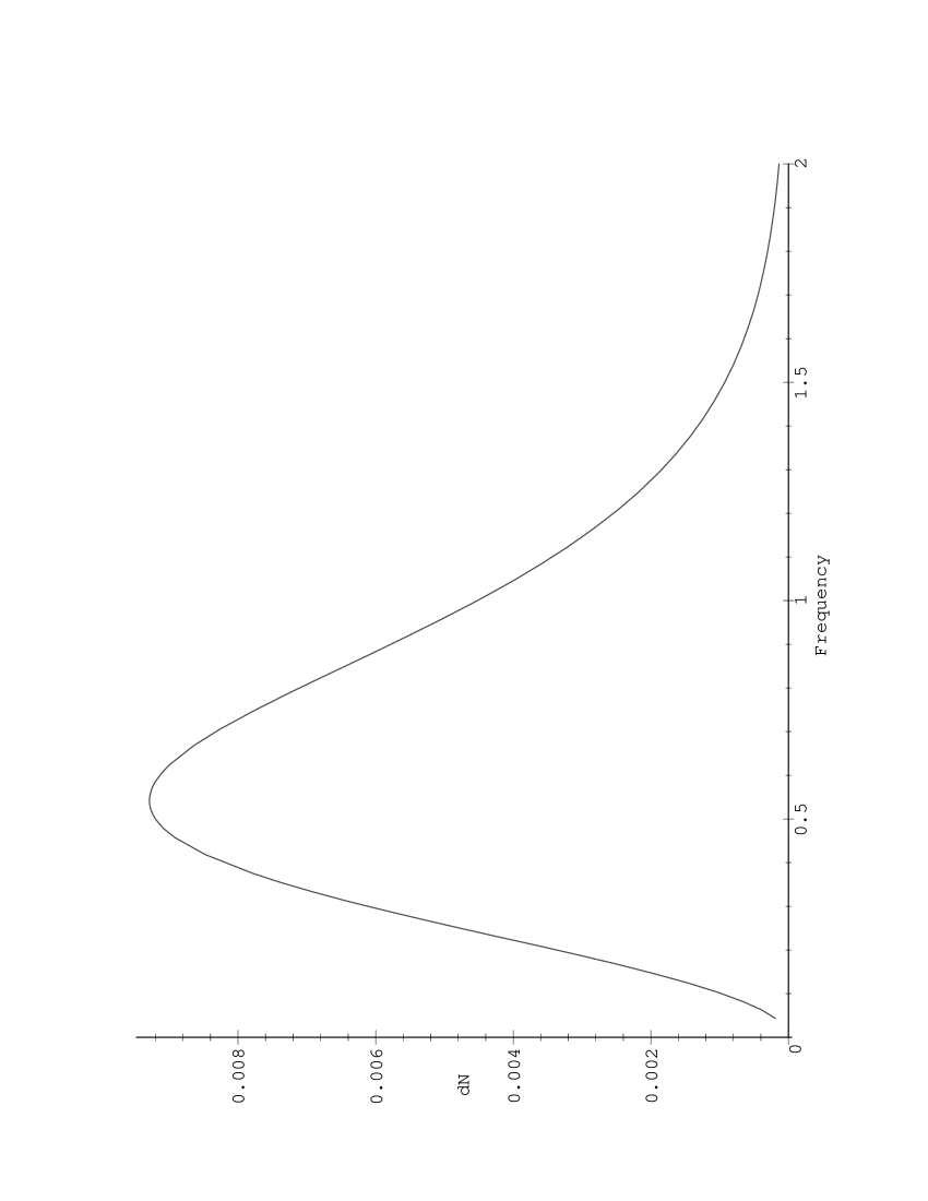
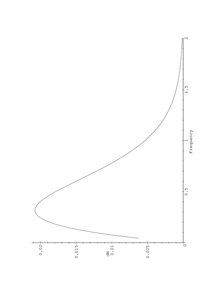
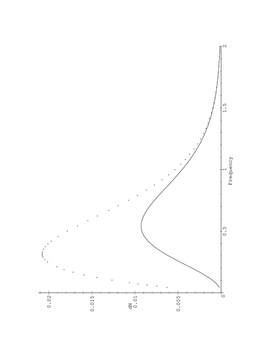
Lessons from this toy model

1. This is only a toy model, but it adequately confirms what we have seen in chapter 1: efficient photon production occurs only when the sudden approximation holds, and that photon production is suppressed in the adiabatic regime. The particular choice of profile $\epsilon(\tau)$ was merely a convenience, it allowed us to get analytic exact results, but it is not a critical part of the analysis. One might worry that the results of this toy model are specific to the choice of profile (4.25). That the results are more general can be established by analyzing general bounds on the Bogoliubov coefficients, which is equivalent to studying general bounds on one-dimensional potential scattering [250]. I shall here quote only the key result that for any monotonic change in the dielectric constant the sudden approximation provides a strict upper bound on the magnitude of the Bogoliubov coefficients [250].

2. Eberlein’s model for Sonoluminescence [231, 232, 233] explicitly uses the adiabatic approximation. For arbitrary adiabatic changes we expect the exponential suppression to still hold with $\rho$ now being some measure of the timescale over which the refractive index changes.

3. Schwinger’s model for Sonoluminescence [224, 225, 226, 227, 228, 229, 230] implicitly uses the sudden approximation. It is only for the sudden approximation that we recover Schwinger’s phase-space limited spectrum. For arbitrary changes the sudden approximation provides a rigorous upper bound on photon production. It is only in the sudden approximation that efficient conversion of zero-point fluctuations to real photons takes place. Though this result is derived here only for a particularly simple toy model one can expect this part of the analysis to be completely generic and that any mechanism for converting zero-point fluctuations to real photons will exhibit similar effects.

4.2.2 Extension of the model

The major weaknesses of the toy model are that it currently includes neither dispersive effects nor finite volume effects. Including dispersive effects amounts to including condensed matter physics by letting the refractive index itself be a function of frequency. To do this carefully requires a very detailed understanding of the condensed matter physics, which is quite beyond the scope of the present investigation. Instead, in this section we shall content ourselves with making order-of-magnitude estimates using Schwinger’s sharp cutoff for the refractive index and the sudden approximation.

The second issue, that of finite volume effects, is addressed more carefully in section 4.3. Finite volume effects are expected to be significant but not overwhelmingly large. From estimates of the available Casimir energy developed in [236], the fractional change in available Casimir energy due to finite volume effects is expected to be of order $1/(KR)=\hbox{(cutoff wavelength)}/(2\pi\hbox{(minimum bubble radius)})$ which is approximately $(300\;\hbox{nm})/(2\pi\;500\;\hbox{nm})\approx 10\%\;$. Returning to dispersive issues: if the refractive indices were completely non-dispersive (frequency-independent), then the sudden approximation would imply infinite energy production. In the real physical situation $n_{\mathrm{in}}$ is a function of $\omega_{\mathrm{in}}$ and $n_{\mathrm{out}}$ is a function of $\omega_{\mathrm{out}}$. Schwinger’s sharp momentum-space cutoff for the refractive index is equivalent, in this formalism, to the choice

$$n_{\mathrm{in}}(k)=n_{\mathrm{in}}\;\Theta(K_{\mathrm{in}}-k)+1\;\Theta(k-K_{\mathrm{in}}),$$ (4.58)

$$n_{\mathrm{out}}(k)=n_{\mathrm{out}}\;\Theta(K_{\mathrm{out}}-k)+1\;\Theta(k-K_{\mathrm{out}}),$$ (4.59)

(More complicated models for the cutoff are of course possible at the cost of obscuring the analytic properties of the model. See [235] for further discussion.) Although in general the two cutoff wavenumbers $K_{\mathrm{in}}$ and $K_{\mathrm{out}}$ can be different, generally they will both lie in the UV range. This allows us to assume a single common cutoff $K\equiv\hbox{min}\{K_{\mathrm{in}},K_{\mathrm{out}}\}$. From equation (4.46), taking into account the two photon polarizations, one obtains

$$|\beta(\vec{k}_{\mathrm{in}},\vec{k}_{\mathrm{out}})|^{2}\approx{1\over 2}\frac{\left(n_{\mathrm{out}}-n_{\mathrm{in}}\right)^{2}}{n_{\mathrm{in}}n_{\mathrm{out}}}{V\over(2\pi)^{3}}\;\Theta(K-k_{\mathrm{in}})\;\Theta(K-k_{\mathrm{out}})\;\delta^{3}(\vec{k}_{\mathrm{in}}+\vec{k}_{\mathrm{out}}).$$ (4.60)

As a consistency check, expression (4.60) has the desirable property that $\beta\to 0$ as $n_{\mathrm{out}}\to n_{\mathrm{in}}$: That is, if there is no change in the refractive index, there is no particle production.

Warning: Equation (4.60) is not the complete Bogoliubov coefficient. We are missing the contribution coming from the case $K_{\mathrm{in}}>K_{\mathrm{out}}$ or $K_{\mathrm{in}}<K_{\mathrm{out}}$. Nevertheless the above cited physical fact, that one can expect $K_{\mathrm{in}}\approx K_{\mathrm{out}}$, makes this contribution negligible with respect to the above one. In any case this approximation amounts to a slight underestimate of the total number of produced photons.

The computed Bogoliubov coefficient is directly related to the physical quantities one is interested in

$${{\mathrm{d}}N\over{\mathrm{d}}\omega_{\mathrm{out}}}=4\pi\frac{n_{\mathrm{out}}^{3}\omega_{\mathrm{out}}^{2}}{c^{3}}\;\int|\beta(\omega_{\mathrm{in}},\omega_{\mathrm{out}})|^{2}\;{\mathrm{d}}^{3}\vec{k}_{\mathrm{in}},$$ (4.61)

$$N=\int{{\mathrm{d}}N\over{\mathrm{d}}\omega_{\mathrm{out}}}\;{\mathrm{d}}\omega_{\mathrm{out}},$$ (4.62)

and

$$E=\hbar\int{{\mathrm{d}}N(\omega_{\mathrm{out}})\over{\mathrm{d}}\omega_{\mathrm{out}}}\;\omega_{\mathrm{out}}\;{\mathrm{d}}\omega_{\mathrm{out}}.$$ (4.63)

So we can now compute the spectrum, the number, and the total energy of the emitted photons.

$${{\mathrm{d}}N(\omega_{\mathrm{out}})\over{\mathrm{d}}\omega_{\mathrm{out}}} = \frac{n_{\mathrm{out}}}{c}\;{{\mathrm{d}}N(\omega_{\mathrm{out}})\over{\mathrm{d}}k_{\mathrm{out}}}=\frac{n_{\mathrm{out}}}{c}\;4\pi k^{2}_{\mathrm{out}}{{\mathrm{d}}N(\omega_{\mathrm{out}})\over{\mathrm{d}}^{3}{\vec{k}}_{\mathrm{out}}}$$

$$\approx {n_{\mathrm{out}}\over(2\;c)}\;{\left(n_{\mathrm{out}}-n_{\mathrm{in}}\right)^{2}\over n_{\mathrm{out}}\,n_{\mathrm{in}}}{V\over(2\pi)^{3}}\;4\pi\;k_{\mathrm{out}}^{2}\;\Theta(K-k_{\mathrm{out}})\;$$

$$= {1\over(2\;c^{3})}\;{n_{\mathrm{out}}^{2}}\;{\left(n_{\mathrm{out}}-n_{\mathrm{in}}\right)^{2}\over n_{\mathrm{in}}}{V\over(2\pi)^{3}}\;4\pi\;\omega_{\mathrm{out}}^{2}\;\Theta\left(K-\frac{n_{\mathrm{out}}\omega_{\mathrm{out}}}{c}\right)$$

The number of emitted photons is then approximately

$$N\approx{1\over 12\pi^{2}}\;{\left(n_{\mathrm{out}}-n_{\mathrm{in}}\right)^{2}\over n_{\mathrm{in}}n_{\mathrm{out}}}\;{VK^{3}}.$$ (4.65)

So that for a spherical bubble

$$N\approx{1\over 9\pi}\;{\left(n_{\mathrm{out}}-n_{\mathrm{in}}\right)^{2}\over n_{\mathrm{out}}n_{\mathrm{in}}}\;(RK)^{3}.$$ (4.66)

It is important to note that the wavenumber cutoff $K$ appearing in the above formula is not equal to the observed wavenumber cutoff $K_{\mathrm{observed}}$. The observed wavenumber cutoff is in fact the upper wavelength measured once the photons have left the bubble and entered the ambient medium (water), so actually

$$K={\omega_{\mathrm{max}}n_{\mathrm{out}}\over c}={n_{\mathrm{out}}\over n_{\mathrm{liquid}}}\;K_{\mathrm{observed}}.$$ (4.67)

Thus

$$N \approx {1\over 9\pi}\;{\left(n_{\mathrm{out}}-n_{\mathrm{in}}\right)^{2}\over n_{\mathrm{out}}n_{\mathrm{in}}}\;\left(R\;{n_{\mathrm{out}}\over n_{\mathrm{liquid}}}\;K_{\mathrm{observed}}\right)^{3}$$ (4.68)

$$= {1\over 9\pi}\;{\left(n_{\mathrm{out}}-n_{\mathrm{in}}\right)^{2}\over n_{\mathrm{in}}}\;n_{\mathrm{out}}^{2}\;\left({R\omega_{\mathrm{max}}\over c}\right)^{3}.$$

The total emitted energy is approximately

$$E \approx \frac{n_{\mathrm{out}}^{2}}{2c^{3}}\;{\left(n_{\mathrm{out}}-n_{\mathrm{in}}\right)^{2}\over n_{\mathrm{in}}}{V\over(2\pi)^{3}}\;4\pi\;\int\hbar\omega_{\mathrm{out}}\;\omega_{\mathrm{out}}^{2}\;\Theta\left(K-\frac{n_{\mathrm{out}}\omega_{\mathrm{out}}}{c}\right){\mathrm{d}}\omega_{\mathrm{out}}$$ (4.69)

$$= {\hbar\over 2}\;\frac{n_{\mathrm{out}}^{2}}{c^{3}}\;{\left(n_{\mathrm{out}}-n_{\mathrm{in}}\right)^{2}\over n_{\mathrm{in}}}\;{V\over(2\pi)^{3}}\;{4\pi\over 4}\;(K\;c/n_{\mathrm{out}})^{4}$$

$$= {1\over 16\pi^{2}}\;{\left(n_{\mathrm{out}}-n_{\mathrm{in}}\right)^{2}\over n_{\mathrm{in}}n_{\mathrm{out}}^{2}}\;\hbar\;c\;K\;{VK^{3}}$$

$$= \frac{3}{4}\;N\;\hbar\omega_{\mathrm{max}}.$$

Taking into account that the maximum photon energy is $\hbar\,\omega_{\mathrm{max}}\approx 4\;{\rm eV}$, the average energy per emitted photon is approximately

$$\langle E\rangle={3\over 4}\hbar c\;K/n_{\mathrm{out}}={3\over 4}\hbar\,\omega_{\mathrm{max}}\sim 3\;{\rm eV}.$$ (4.70)

Taking into account this extra factor we can now consider some numerical estimates based on our results.

4.2.3 Some numerical estimates

In Schwinger’s original model he took $n_{\mathrm{gas}}^{\mathrm{in}}\approx 1$, $n_{\mathrm{gas}}^{\mathrm{out}}\approx n_{\mathrm{liquid}}\approx 1.3$, $V=(4\pi/3)R^{3}$, with $R\approx R_{\mathrm{max}}\approx 40\;\mu{\rm m}$ and $K\approx 2\pi/(360\;{\rm nm})$ [227]. Then $KR\approx 698$. Substitution of these numbers into equation (4.1) leads to an energy budget suitable for about three million emitted photons.

By direct substitution in equation (4.69) it is easy to check that Schwinger’s results can qualitatively be recovered also in our formalism: in our case we get about 1.8 million photons for the same numbers of Schwinger and about 4 million photons using the updated experimental figures $R_{\mathrm{max}}\approx 45\;\mu{\rm m}$ and $K\approx 2\pi/(300\;{\rm nm})$.

A sudden change in refractive index would indeed convert the most of the energy budget based on static Casimir energy calculations into real photons. This may be interpreted as an independent check on Schwinger’s estimate of the Casimir energy of a dielectric sphere. Unfortunately, the sudden (femtosecond) change in refractive index required to get efficient photon production is also the fly in the ointment that kills Schwinger’s original choice of parameters: The collapse from $R_{\mathrm{max}}$ to $R_{\mathrm{min}}$ is known to require approximately $10\;{\rm ns}$, which is far too long a timescale to allow us to adopt the sudden approximation.

In the new version of the model presented here one has $R\approx R_{\mathrm{light-emitting-region}}\approx R_{\mathrm{min}}\approx 500\;\hbox{nm}$ and take $K_{\mathrm{observed}}\approx 2\pi/(200\;{\mathrm{nm}})$ so that $K_{\mathrm{observed}}R\approx 5\pi\approx 15$. To get about one million photons one now needs, for instance, $n_{\mathrm{in}}\approx 1$ and $n_{\mathrm{out}}\approx 12$, or $n_{\mathrm{in}}\approx 2\times 10^{4}$ and $n_{\mathrm{out}}\approx 1$, or even $n_{\mathrm{out}}\approx 25$ and $n_{\mathrm{in}}\approx 71$, though many other possibilities could be envisaged. In particular, the first set of values could correspond to a change of the refractive index at the van der Waals hard core due to a sudden compression e.g., generated by a shock wave. In this framework it is obvious that the most favorable composition for the gas would be a noble gas since this mechanism would be most effective if the gas could be enormously compressed without being easily ionizable.

Note that the estimated values of $n_{\mathrm{gas}}^{\mathrm{out}}$ and $n_{\mathrm{gas}}^{\mathrm{in}}$ are extremely sensitive to the precise choice of cutoff, and the size of the light emitting region, and that the approximations used in taking the infinite volume limit underlying the use of our homogeneous dielectric model are uncontrolled. We should not put to much credence in the particular numerical value of $n_{\mathrm{gas}}^{\mathrm{out}}$ estimated by these means, but should content ourselves with this qualitative message: one needs the refractive index of the contents of the gas bubble to change dramatically and rapidly to generate the photons.

As a final remark it is important to stress that equation (4.1) and equation (4.69) are not quite identical. The volume term for photon production that we have just derived [equation (4.69)] is of second order in $(n_{\mathrm{in}}-n_{\mathrm{out}})$ and not of first order like equation (4.1). This is ultimately due to the fact that the interaction term responsible for converting the initial energy in photons is a pairwise squeezing operator (see [19]). Equation (4.69) demonstrates that any argument that attempts to deny the relevance of volume terms to Sonoluminescence due to their dependence on $(n_{\mathrm{in}}-n_{\mathrm{out}})$ has to be carefully reassessed. In fact what you measure when the refractive index in a given volume of space changes is not directly the change in the static Casimir energy of the “in” state, but rather the fraction of this static Casimir energy that is converted into photons. We have just seen that once conversion efficiencies are taken into account, the volume dependence is conserved, but not the power in the difference of the refractive index. Indeed the dependence of $|\beta|^{2}$ on $(n_{\mathrm{in}}-n_{\mathrm{out}})^{2}$, and the symmetry of the former under the interchange of “in” and “out” states, also proves that it is the amount of change in the refractive index and not its “direction” that governs particle production. This apparent paradox is easily solved by taking into account that the main source of energy is the acoustic field and that the amount of this energy actually converted in photons during each cycle is a very small fraction of the total acoustic energy.

Estimate of the number of photons

Using the above as a guide to the appropriate starting point, we can now systematically explore the relationship between the in and out refractive indexes and the number of photons produced. Using $K_{\mathrm{observed}}R\approx 15$ one gets

$$N={119\over n_{\mathrm{liquid}}^{3}}\;(n_{\mathrm{out}}-n_{\mathrm{in}})^{2}\;{n_{\mathrm{out}}^{2}\over n_{\mathrm{in}}}.$$ (4.71)

This equation can be algebraically solved for $n_{\mathrm{in}}$ as a function of $n_{\mathrm{out}}$ and $N$. (It’s a quadratic.) For $N=10^{6}$ emitted photons the result is plotted in figure (4.7). For any specified value of $n_{\mathrm{out}}$ there are exactly two values of $n_{\mathrm{in}}$ that lead to one million emitted photons. To understand the qualitative features of this diagram we can consider three sub-regions.

Figure 4.7: The initial refractive index $n_{\mathrm{in}}$ plotted as a function of $n_{\mathrm{out}}$ when one million photons are emitted in the sudden approximation.

First, if $n_{\mathrm{in}}\ll n_{\mathrm{out}}$ then we can approximate

$$n_{\mathrm{in}}\approx{119\;n_{\mathrm{out}}^{4}\over n_{\mathrm{liquid}}^{3}\;N}.$$ (4.72)

This corresponds to the region near the origin, and one can focus on this region in figure (4.8).

Figure 4.8: The initial refractive index $n_{\mathrm{in}}$ plotted as a function of $n_{\mathrm{out}}$ when one million photons are emitted in the sudden approximation. Here we focus on the branch that approaches the origin.

Second, if $n_{\mathrm{in}}\gg n_{\mathrm{out}}$ then one can approximate

$$n_{\mathrm{in}}\approx{n_{\mathrm{liquid}}^{3}\;N\over 119\;n_{\mathrm{out}}^{2}}.$$ (4.73)

This corresponds to the region near the $y$ axis, and this region is illustrated in figure (4.9).

Figure 4.9: The initial refractive index $n_{\mathrm{in}}$ plotted as a function of $n_{\mathrm{out}}$ when one million photons are emitted in the sudden approximation. Here we focus on the branch that approaches the $y$ axis.

Third, if $n_{\mathrm{in}}\approx n_{\mathrm{out}}$ then one can approximate

$$N\approx{119\over n_{\mathrm{liquid}}^{3}}\;(n_{\mathrm{in}}-n_{\mathrm{out}})^{2}\;n_{\mathrm{out}},$$ (4.74)

so that

$$n_{\mathrm{in}}\approx n_{\mathrm{out}}\pm\sqrt{N\;n_{\mathrm{liquid}}^{3}\over 119\;n_{\mathrm{out}}}.$$ (4.75)

This corresponds to the region near the asymptote $n_{\mathrm{in}}=n_{\mathrm{out}}$.

Thus to get a million photons emitted from the van der Waals hard core in the sudden approximation requires a significant (but not enormous) change in refractive index. There are many possibilities consistent with the present model and the experimental data.

Estimate of the timescale

We have already seen that the actual physical timescale required for getting a non-adiabatically-suppressed spectrum up to femtosecond frequencies is given by formula (4.44). This is indeed rather different from the simple inverse of $\Omega_{\mathrm{sudden}}$, being a function of both the sudden cutoff frequency and the refractive indices: $t_{0}=F(\Omega_{\mathrm{sudden}},n_{\mathrm{in}},n_{\mathrm{out}})$.

Fixing $\Omega_{\mathrm{sudden}}=1\;{\rm PHz}$ we can easily plot $t_{0}$ as a function of $n_{\mathrm{in}}$ and $n_{\mathrm{out}}$. From the following graphs it is easy to see that there is a large range of values for the refractive indices for which $t_{0}\gg 1\;{\rm fs}$. In particular the case $n_{\mathrm{in}}\approx 2\;10^{4}$, $n_{\mathrm{out}}\approx 1$, would permit a rather relaxed timescale of just $t_{0}\approx 6.4\;{\rm ps}$ in order to get 1 million photons and a spectrum rising up to 1 PHz.

Figure 4.10: Plot of $t_{0}$ as a function of $n_{\mathrm{in}}$ and $n_{\mathrm{out}}$ with $\Omega_{\mathrm{sudden}}=1$PHz. The units on the $t_{0}$ axis are femtoseconds. The plotted range is range $1<n_{\mathrm{in}}<3\;10^{4}$ and $1<n_{\mathrm{out}}<30$. The plane underneath corresponds to $t_{0}\equiv 1\;{\rm fs}$.

Figure 4.11: Plot of $t_{0}$ as a function of $n_{\mathrm{in}}$ and $n_{\mathrm{out}}$ with $\Omega_{\rm sudden}=1$PHz. The units on the $t_{0}$ axis are femtoseconds. The plotted range is $1<n_{\mathrm{in}}<10^{5}$ and $1<n_{\mathrm{out}}<10^{4}$. The horizontal plane corresponds to $t_{0}\equiv 1\;{\rm fs}$.

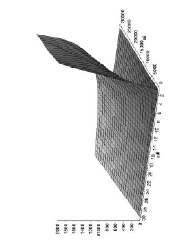
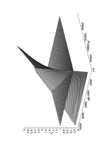
These results, while encouraging, should be taken with some caution. Equation (4.44) is actually dependent on the temporal profile we choose for the change in the refractive index. Furthermore, the precise values of the refractive indices depend sensitively on other aspects of the model. To fix these uncertainties one requires a fully developed condensed matter analysis (either by simulation or direct measurement) able to provide a detailed dynamics for the refractive index under the rather extreme conditions encountered at the van der Waals bounce. No such analysis is currently extant, or even practical.

So far in order to keep that discussion tractable, the technical computations have been limited to the case of a homogeneous dielectric medium. We shall now investigate the additional complications introduced by finite-volume effects. The basic physical scenario remains the same, but we shall now deal with finite spherical bubbles. We shall see how to set up the formalism for calculating Bogoliubov coefficients in the sudden approximation, and show that one qualitatively retains the results previously obtained using the homogeneous-dielectric (infinite volume) approximation.

4.3 Sonoluminescence as a dynamical Casimir effect: Finite Volume model

In this case our strategy will be analogous the subtraction procedure of the static calculations of Schwinger [224, 225, 226, 227, 228, 229, 230] or of Carlson et al. [234, 235, 236] we shall consider two different configurations. An “in” configuration with a bubble of refractive index $n_{\mathrm{gas}}^{\mathrm{in}}$ in a medium of dielectric constant $\epsilon_{{\mathrm{outside}}}$, and an “out” configuration with a bubble of refractive index $n_{\mathrm{gas}}^{\mathrm{out}}$ in a medium of dielectric constant $\epsilon_{{\mathrm{outside}}}$. These two configurations will correspond to two different bases for the quantization of the field. (For the sake of simplicity we can take, as Schwinger did, only the electric part of QED, reducing the problem to a scalar electrodynamics). The two bases will be related by Bogoliubov coefficients in the usual way. Once we determine these coefficients we easily get the number of created particles per mode, and from this the spectrum.

Let us adopt the Schwinger formalism and consider the equations of the electric field in spherical coordinates and with a time-independent dielectric constant. (We can temporarily set $c=1$ for ease of notation, and shall reintroduce appropriate factors of the speed of light when needed for clarity.) Then in the asymptotic future and asymptotic past, where the refractive index is taken to be time-independent, we are interested in solving

$$\epsilon(r)\;\partial_{0}(\partial_{0}E)-\nabla^{2}E=0,$$ (4.76)

with $\epsilon(r)$ being piecewise constant. We can look for solutions of the form

$$E=\Phi(r,t)\;Y_{lm}(\Omega)\;{1\over r}.$$ (4.77)

Then one finds

$$\epsilon(\partial^{2}_{0}\Phi)-(\partial_{r}^{2}\Phi)+{1\over r^{2}}l(l+1)\Phi=0.$$ (4.78)

For both the “in” and “out” solution the field equation in $r$ is given by:

$$\epsilon\partial_{0}^{2}\Phi-\partial_{r}^{2}\Phi+{1\over r^{2}}l(l+1)\Phi=0.$$ (4.79)

In both asymptotic regimes (past and future) one has a static situation (a bubble of dielectric $n_{\mathrm{gas}}^{\mathrm{in}}$ in the dielectric $n_{\mathrm{liquid}}$, or a bubble of dielectric $n_{\mathrm{gas}}^{\mathrm{out}}$ in the dielectric $n_{\mathrm{liquid}}$) so one can in this limit factorize the time and radius dependence of the modes: $\Phi(r,t)=e^{{\mathrm{i}}\omega t}f(r)$. One gets

$$f^{{}^{\prime\prime}}+\left(\epsilon\omega^{2}-{1\over r^{2}}l(l+1)\right)f=0.$$ (4.80)

This is a well known differential equation. To handle it more easily in a standard way we can cast it as an eigenvalues problem

$$f^{{}^{\prime\prime}}-\left({1\over r^{2}}l(l+1)\right)f=-\varpi^{2}f,$$ (4.81)

where $\varpi^{2}=\epsilon\omega^{2}$. With the change of variables $f=r^{1/2}G$, so that $\Phi(r,t)=e^{{\mathrm{i}}\omega t}r^{1/2}G(r)$, one gets

$$G^{{}^{\prime\prime}}+{1\over r}G^{{}^{\prime}}+\left(\varpi^{2}-{\nu^{2}\over r^{2}}\right)G=0.$$ (4.82)

This is the standard Bessel equation. It admits as solutions the Bessel and Neumann functions of the first type, $J_{\nu}(\varpi r)$ and $N_{\nu}(\varpi r)$, with $\nu=l+1/2$. Remember that for those solutions which have to be well-defined at the origin, $r=0$, regularity implies the absence of the Neumann functions. For both the “in” and the “out” basis one has to take into account that the dielectric constant changes at the bubble radius ($R$). In fact one has

$$\epsilon^{\mathrm{in}}=\left\{\begin{array}[]{llllll}\vphantom{\Bigg{|}}\epsilon_{\mathrm{inside}}^{\mathrm{in}}&=&(n_{\mathrm{gas}}^{\mathrm{in}})^{2}&=&\mbox{\small dielectric constant of air-gas mixture}&\mbox{if $r\leq R$},\\ \vphantom{\Bigg{|}}\epsilon_{\mathrm{outside}}^{\mathrm{in}}&=&n^{2}_{\mathrm{liquid}}&=&\mbox{\small dielectric constant of ambient liquid}&\mbox{if $r>R$}.\end{array}\right.$$ (4.83)

After the change in refractive index, one gets

$$\epsilon^{\mathrm{out}}=\left\{\begin{array}[]{llllll}\vphantom{\Bigg{|}}\epsilon_{\mathrm{inside}}^{\mathrm{out}}&=&(n_{\mathrm{gas}}^{\mathrm{out}})^{2}&=&\mbox{\small dielectric constant of air-gas mixture}&\mbox{if $r\leq R$},\\ \vphantom{\Bigg{|}}\epsilon_{\mathrm{outside}}^{\mathrm{out}}&=&n^{2}_{\mathrm{liquid}}&=&\mbox{\small dielectric constant of ambient liquid}&\mbox{if $r>R$}.\end{array}\right.$$ (4.84)

Defining the “in” and “out” frequencies, $\omega_{\mathrm{in}}$ and $\omega_{\mathrm{out}}$ respectively, one has

$$G^{\mathrm{in}}_{\nu}(n_{\mathrm{gas}}^{\mathrm{in}},n_{\mathrm{liquid}},\omega_{\mathrm{in}},r)=\left\{\begin{array}[]{ll}\vphantom{\Bigg{|}}\Xi_{\nu}^{\mathrm{in}}\;A_{\nu}^{\mathrm{in}}\;J_{\nu}(n_{\mathrm{gas}}^{\mathrm{in}}\,\omega_{\mathrm{in}}r)&\mbox{if $r\leq R$},\\ \vphantom{\Bigg{|}}\Xi_{\nu}^{\mathrm{in}}\;\left[B_{\nu}^{\mathrm{in}}\;J_{\nu}(n_{\mathrm{liquid}}\,\omega_{\mathrm{in}}r)+C_{\nu}^{\mathrm{in}}\;N_{\nu}(n_{\mathrm{liquid}}\,\omega_{\mathrm{in}}r)\right]&\mbox{if $r>R$.}\end{array}\right.$$ (4.85)

Here $\Xi_{\nu}^{\mathrm{in}}$ is an overall normalization. The $A_{\nu}^{\mathrm{in}}$, $B_{\nu}^{\mathrm{in}}$, and $C_{\nu}^{\mathrm{in}}$ coefficients are determined by the matching conditions at $R$

$$\begin{array}[]{lll}\vphantom{\Bigg{|}}A_{\nu}^{\mathrm{in}}\;J_{\nu}(n_{\mathrm{gas}}^{\mathrm{in}}\,\omega_{\mathrm{in}}R)&=&B_{\nu}^{\mathrm{in}}\;J_{\nu}(n_{\mathrm{liquid}}\,\omega_{\mathrm{in}}R)+C_{\nu}^{\mathrm{in}}\;N_{\nu}(n_{\mathrm{liquid}}\,\omega_{\mathrm{in}}R),\\ \vphantom{\Bigg{|}}A_{\nu}^{\mathrm{in}}\;J_{\nu}{{}^{\prime}}(n_{\mathrm{gas}}^{\mathrm{in}}\,\omega_{\mathrm{in}}R)&=&B_{\nu}^{\mathrm{in}}\;J_{\nu}{{}^{\prime}}(n_{\mathrm{liquid}}\,\omega_{\mathrm{in}}R)+C_{\nu}^{\mathrm{in}}\;N_{\nu}{{}^{\prime}}(n_{\mathrm{liquid}}\,\omega_{\mathrm{in}}R),\end{array}$$ (4.86)

(the primes above denote derivatives with respect to $r$), together with the convention that

$$|B|^{2}+|C|^{2}=1$$ (4.87)

The “out” basis is easily obtained solving the same equations but systematically replacing $n_{\mathrm{gas}}^{\mathrm{in}}$ by $n_{\mathrm{gas}}^{\mathrm{out}}$. There will be additional coefficients, $\Xi_{\nu}^{\mathrm{out}}$, $A_{\nu}^{\mathrm{out}}$, $B_{\nu}^{\mathrm{out}}$, and $C_{\nu}^{\mathrm{out}}$, corresponding to the “out” basis.

To proceed further we now need to spend some words about the way the inner product must be generalized in the case of time-dependent and space-dependent refractive index. This will allow us to impose the normalization conditions on the $\Phi$ functions and fix the $\Xi_{\nu}$ coefficients.

4.3.1 Generalizing the inner product

For the differential equation

$$\epsilon\;\partial_{0}(\partial_{0}E)-\nabla^{2}E=0,$$ (4.88)

it is a standard exercise to write down a density and flux,

$$\rho=\epsilon\left(E_{1}^{*}\;\partial_{t}E_{2}-E_{2}\;\partial_{t}E_{1}^{*}\right),$$ (4.89)

$$j=E_{1}^{*}\nabla E_{2}-E_{2}\nabla E^{*}_{1},$$ (4.90)

and to then show that, by virtue of the differential equation (4.88), these quantities satisfy a continuity equation

$$\partial_{t}\rho-\nabla\cdot j=0.$$ (4.91)

Suppose now one has two solutions of the differential equation (4.88), one can then define an inner product

$$(E_{1},E_{2})=-{\mathrm{i}}\;\epsilon\int_{t}\left(E^{*}_{1}\partial_{t}E_{2}-E_{2}\partial_{t}E_{1}^{*}\right),$$ (4.92)

where the integral is taken over a constant-time spacelike hypersurface. By virtue of the above, this inner product is independent of the time $t$ at which it is evaluated.

Now what happens if the dielectric is allowed to depend on both space and time? First the differential equation of interest is generalized to

$$\partial_{0}(\epsilon(x,t)\partial_{0}E)-\nabla^{2}E=0.$$ (4.93)

Second, the density and flux become,

$$\rho=\epsilon(r,t)\left(E_{1}^{*}\partial_{t}E_{2}-E_{2}\partial_{t}E_{1}^{*}\right),$$ (4.94)

$$j=E_{1}^{*}\nabla E_{2}-E_{2}\nabla E_{1}^{*}.$$ (4.95)

By virtue of the differential equation (4.93),

$$\partial_{t}\rho \equiv E_{1}^{*}\;\partial_{t}\left(\epsilon(x,t)\partial_{t}E_{2}\right)-E_{2}\;\partial_{t}\left(\epsilon(x,t)\partial_{t}E_{1}^{*}\right)$$ (4.96)

$$= E_{1}^{*}\nabla^{2}E_{2}-E_{2}\nabla^{2}E_{1}^{*}$$ (4.97)

$$= \nabla\cdot\left(E_{1}^{*}\nabla E_{2}-E_{2}\nabla E_{1}^{*}\right)$$ (4.98)

$$= \nabla\cdot j.$$ (4.99)

Which implies that these generalized quantities satisfy a continuity equation

$$\partial_{t}\rho-\nabla\cdot j=0.$$ (4.100)

This implies that the generalized inner-product [for two solutions $E_{1}$ and $E_{2}$ of the equation (4.93) for time-dependent and space-dependent dielectric constants] must be

$$(E_{1},E_{2})=-{\mathrm{i}}\int_{t}\epsilon(x,t)\left(E^{*}_{1}\partial_{t}E_{2}-E_{2}\partial_{t}E_{1}^{*}\right).$$ (4.101)

By the continuity equation this inner product is independent of the time $t$ at which the integral is evaluated [provided of course, that $E_{1}$ and $E_{2}$ both satisfy (4.93)]. This construction can be made completely relativistic. Define a four-vector $J^{\mu}$ by

$$J^{\mu}\equiv(\rho;j^{i}).$$ (4.102)

Then for any edgeless achronal spacelike hypersurface $\Sigma$ there is a conserved inner product

$$(E_{1},E_{2})=-{\mathrm{i}}\;\int_{\Sigma}\epsilon(x,t)\;J^{\mu}\;{\mathrm{d}}\Sigma_{\mu}.$$ (4.103)

4.3.2 Fixing the normalization constants

One can now demand the existence of a normalized scalar product such that one can define orthonormal eigenfunctions

$$\left(\Phi^{i},\Phi^{j}\right)=\delta^{ij}.$$ (4.104)

For the special case $n_{\mathrm{gas}}=n_{\mathrm{liquid}}$, (corresponding to a completely homogeneous space, in which case $A=1=B$, $C=0$), Eq. 4.101 takes the trivial form (which was implicitly in Eq. 4.27)

$$\left(\phi_{1},\phi_{2}\right)={\mathrm{i}}\,n^{2}\int_{\Sigma_{t}}\phi_{1}^{*}\stackrel{{\scriptstyle\leftrightarrow}}{{\partial}}_{0}\phi_{2}\>{\mathrm{d}}^{3}x,$$ (4.105)

If we now take the scalar product of two eigenfunctions, we expect to obtain a normalization condition which can be written as

$$\left(\Phi^{i}_{[n_{\mathrm{gas}}=n_{\mathrm{liquid}}]},\Phi^{j}_{[n_{\mathrm{gas}}=n_{\mathrm{liquid}}]}\right)=\delta^{ij}.$$ (4.106)

Inserting the explicit form of the $\Phi$ functions one gets 

$$\left(\Phi^{i}_{[n_{\mathrm{gas}}=n_{\mathrm{liquid}}]},\Phi^{j}_{[n_{\mathrm{gas}}=n_{\mathrm{liquid}}]}\right)=2\;\Xi_{i}^{*}\;\Xi_{j}\;\delta_{ll^{\prime}}\;\delta_{mm^{\prime}}\;n\;\delta(\varpi_{i}-\varpi_{j}),$$ (4.108)

One can now compare this to the behaviour of the three-dimensional delta function in momentum space

$$\delta^{3}(\vec{\varpi}_{i}-\vec{\varpi}_{j}) = {\delta(\varpi_{i}-\varpi_{j})\over\varpi_{i}\;\varpi_{j}}\;\delta^{2}(\hat{\varpi}_{i}-\hat{\varpi}_{j})$$ (4.109)

$$= {\delta(\varpi_{i}-\varpi_{j})\over\varpi_{i}\;\varpi_{j}}\;\sum_{lm}Y^{*}_{lm}(\theta_{i},\phi_{i})\;Y_{lm}(\theta_{j},\phi_{j})$$ (4.110)

$$\to {\delta(\varpi_{i}-\varpi_{j})\over\varpi_{i}\;\varpi_{j}}\;\delta_{ll^{\prime}}\;\delta_{mm^{\prime}},$$ (4.111)

to deduce that for homogeneous spaces the most useful normalization is

$$2\;\Xi_{i}^{*}\;\Xi_{j}\;n={1\over\varpi_{i}\;\varpi_{j}}.$$ (4.112)

This strongly suggests that even for static but non-homogeneous dielectric configurations it will be advantageous to set

$$\left|\,\Xi^{i}\right|={1\over\sqrt{2n}\;\varpi_{i}}.$$ (4.113)

where $n$ is now the refractive index at spatial infinity 

To confirm that this is still the most appropriate normalization for non-homogeneous dielectrics requires a careful discussion which can be found in [18]. The central result is that it is indeed the refractive index at spatial infinity the relevant one for this overall normalization. So, if one adopts the convention that

$$|B|^{2}+|C|^{2}=1,$$ (4.114)

then proper normalization of the wavefunctions demands

$$\left|\Xi^{i}\right|={1\over\sqrt{2\,n_{\mathrm{liquid}}}\;\varpi_{i}},$$ (4.115)

4.3.3 Finite volume calculation

We are now ready to ask what happens if we change the refractive index by making $\epsilon(r,t)$ a function of both position and time. We are interested in solving the equation (4.93) and from the previous discussion it should now be clear that the inner product must now be modified (in what is now a rather obvious fashion).

$$\left(\phi_{1},\phi_{2}\right)={\mathrm{i}}\,\int_{\Sigma_{t}}\epsilon(r,t)\;\phi_{1}^{*}\stackrel{{\scriptstyle\leftrightarrow}}{{\partial}}_{0}\phi_{2}\>{\mathrm{d}}^{3}x,$$ (4.116)

The Bogoliubov coefficients (relative to this inner product) can now be defined as

$$\alpha_{ij} = -\left({E_{i}^{\mathrm{out}}},{E_{j}^{\mathrm{in}}}\right),$$ (4.117)

$$\beta_{ij} = \left({E_{i}^{\mathrm{out}}}^{*},{E_{j}^{\mathrm{in}}}\right).$$ (4.118)

Where $E_{j}^{\mathrm{in}}$ now denotes an exact solution of the time-dependent equation (4.93) that in the infinite past approaches a solution of the static equation (4.76) with $\epsilon\to\epsilon_{\mathrm{in}}(r)$ and eigen-frequency $\omega_{j}$. Similarly $E_{i}^{\mathrm{out}}$ now denotes an exact solution of the time-dependent equation (4.93) that in the infinite future approaches a solution of the static equation (4.76) with $\epsilon\to\epsilon_{\mathrm{out}}(r)$ and eigen-frequency $\omega_{i}$. The inner product used to define the Bogoliubov coefficients has been carefully arranged to correspond to a “conserved charge”. With the conventions we have in place the absolute values of the Bogoliubov coefficient are independent of the choice of time-slice $\Sigma_{t}$ on which the spatial integral is evaluated. With minor modifications, as explained in section 4.3.1, the inner product can further be generalized to enable it to be defined for any arbitrary edgeless achronal spacelike hypersurface, not just the constant time time-slices. (This whole formalism is very closely related to the S-matrix formalism of quantum field theories, where the S-matrix relates asymptotic “in” and “out” states.)

Of course, evaluating the Bogoliubov coefficients involves solving the exact time-dependent problem (4.93), subject to the specified boundary conditions, a task that is in general very difficult. It is at this stage that we shall explicitly invoke the sudden approximation by choosing the dielectric constant to be

$$\epsilon(r,t)=\epsilon_{\mathrm{in}}(r)\;\Theta(-t)+\epsilon_{\mathrm{out}}(r)\;\Theta(t).$$ (4.119)

This is a simple step-function transition from $\epsilon_{\mathrm{in}}(r)$ to $\epsilon_{\mathrm{out}}(r)$ at time $t=0$. For $t<0$ the exact eigenstates are given in terms of the static problem with $\epsilon=\epsilon_{\mathrm{in}}(r)$, and for $t>0$ the exact eigenstates are given in terms of the static problem with $\epsilon=\epsilon_{\mathrm{out}}(r)$. To evaluate the Bogoliubov coefficients in the simplest manner, we can chose the spacelike hypersurface to be the $t=0$ hyperplane. The inner product then reduces to

$$(\phi_{1},\phi_{2})={\mathrm{i}}\;\int_{t=0}\epsilon(r,t=0)\;\phi_{1}^{*}\stackrel{{\scriptstyle\leftrightarrow}}{{\partial}}_{0}\phi_{2}\>{\mathrm{d}}^{3}x,$$ (4.120)

with the relevant eigenmodes being those of the static “in” and “out” problems. (At a fundamental level, this formalism is just a slight modification of the standard machinery of the sudden approximation in quantum mechanical perturbation theory.)
There is actually a serious ambiguity hiding here: What value are we to assign to $\epsilon(r,t=0)$? One particularly simple candidate is

$$\epsilon(r,t=0)\to{\textstyle{1\over 2}}\left[\epsilon_{\mathrm{in}}(r)+\epsilon_{\mathrm{out}}(r)\right]={\textstyle{1\over 2}}\left[n_{\mathrm{in}}(r)^{2}+n_{\mathrm{out}}(r)^{2}\right],$$ (4.121)

but this candidate is far from unique. For instance, we could rewrite (4.119) as

$$\epsilon(r,t)=\exp\Big{(}\ln\{\epsilon_{\mathrm{in}}(r)\}\;\Theta(-t)+\ln\{\epsilon_{\mathrm{out}}(r)\}\;\Theta(t)\Big{)}.$$ (4.122)

For $t\neq 0$ this is identical to (4.119), but for $t=0$ this would more naturally lead to the prescription

$$\epsilon(r,t=0)\to\sqrt{\epsilon_{\mathrm{in}}(r)\epsilon_{\mathrm{out}}(r)}=n_{\mathrm{in}}(r)n_{\mathrm{out}}(r).$$ (4.123)

By making a comparison with the analytic calculation for homogeneous media presented in section 4.2 it is in fact possible to show that this is the correct prescription [18]. For the moment it is nevertheless convenient to adopt the notation

$$\epsilon(r,t=0)=\gamma\left(n_{\mathrm{in}}(r);n_{\mathrm{out}}(r)\right),$$ (4.124)

where the only property of $\gamma(n_{1};n_{2})$ that we really need to use at this stage is that when $n_{1}=n_{2}$

$$\gamma(n;n)=n^{2}.$$ (4.125)

(This property follows automatically from considering the static time-independent case.)

We are mainly interested in the Bogoliubov coefficient $\beta$, since it is $|\beta|^{2}$ that is linked to the total number of particles created. By a direct substitution it is easy to find the expression:

$$\beta_{ll^{\prime},mm^{\prime}}(\omega_{\mathrm{in}},\omega_{\mathrm{out}})=$$

$$\quad={\mathrm{i}}\int_{0}^{\infty}\gamma\left(n_{\mathrm{in}}(r),n_{\mathrm{out}}(r)\right)\left(\Phi_{\mathrm{out}}(r,t)\;Y_{lm}(\Omega)\;{1\over r}\right)\stackrel{{\scriptstyle\leftrightarrow}}{{\partial}}_{0}\left(\Phi_{\mathrm{in}}(r,t)\;Y_{l^{\prime}m^{\prime}}(\Omega)\;{1\over r}\right)\>r^{2}{\mathrm{d}}r{\mathrm{d}}\Omega,$$

$$\quad=-(\omega_{\mathrm{in}}-\omega_{\mathrm{out}})\;e^{{\mathrm{i}}(\omega_{\mathrm{out}}+\omega_{\mathrm{in}})t}\delta_{ll^{\prime}}\;\delta_{m,-m^{\prime}}\;$$

$$\quad\quad\times\int_{0}^{\infty}\gamma\left(n_{\mathrm{in}}(r);n_{\mathrm{out}}(r)\right)\;G^{\mathrm{out}}_{l}(n_{\mathrm{gas}}^{\mathrm{out}},n_{\mathrm{liquid}},\omega_{\mathrm{out}},r)\;G^{\mathrm{in}}_{l^{\prime}}(n_{\mathrm{gas}}^{\mathrm{in}},n_{\mathrm{liquid}},\omega_{\mathrm{in}},r)\>r{\mathrm{d}}r.$$ (4.126)

(The $\delta_{m,-m^{\prime}}$ arises because of the absence of a relative complex conjugation in the angular integrals for $\beta$ or alternatively can be seen as a consequence of the conservation of angular momentum. On the other hand, the $\alpha$ coefficient will be proportional to $\delta_{mm^{\prime}}$.) To compute the radial integral one needs some ingenuity, let us write the equations of motion for two different values of the eigenvalues, $\varpi_{1}$ and $\varpi_{2}$.

$$G_{\varpi_{1}}^{{}^{\prime\prime}}+{1\over r}G_{\varpi_{1}}^{{}^{\prime}}+\left(\varpi_{1}^{2}-{1\over r^{2}}(l+{\textstyle{1\over 2}})^{2}\right)G_{\varpi_{1}} = 0,$$ (4.127)

$$G_{\varpi_{2}}^{{}^{\prime\prime}}+{1\over r}G_{\varpi_{2}}^{{}^{\prime}}+\left(\varpi_{2}^{2}-{1\over r^{2}}(l+{\textstyle{1\over 2}})^{2}\right)G_{\varpi_{2}} = 0.$$ (4.128)

By multiplying the first by $G_{\varpi_{2}}$ and the second by $G_{\varpi_{1}}$ one gets

$$G_{\varpi_{1}}^{{}^{\prime\prime}}G_{\varpi_{2}}+{1\over r}G_{\varpi_{1}}^{{}^{\prime}}G_{\varpi_{2}}+\left(\varpi_{1}^{2}-{1\over r^{2}}(l+{\textstyle{1\over 2}})^{2}\right)G_{\varpi_{1}}G_{\varpi_{2}} = 0,$$ (4.129)

$$G_{\varpi_{2}}^{{}^{\prime\prime}}G_{\varpi_{1}}+{1\over r}G_{\varpi_{2}}^{{}^{\prime}}G_{\varpi_{1}}+\left(\varpi_{2}^{2}-{1\over r^{2}}(l+{\textstyle{1\over 2}})^{2}\right)G_{\varpi_{1}}G_{\varpi_{1}} = 0.$$ (4.130)

Subtracting the second from the first we then obtain

$$\left(G_{\varpi_{1}}^{{}^{\prime\prime}}G_{\varpi_{2}}-G_{\varpi_{2}}^{{}^{\prime\prime}}G_{\varpi_{1}}\right)+{1\over r}\left(G_{\varpi_{1}}^{{}^{\prime}}G_{\varpi_{2}}-G_{\varpi_{2}}^{{}^{\prime}}G_{\varpi_{1}}\right)+(\varpi_{2}^{2}-\varpi_{1}^{2})G_{\varpi_{1}}G_{\varpi_{2}}=0.$$ (4.131)

The second term on the left hand side is a pseudo–Wronskian determinant

$$W_{\varpi_{1}\varpi_{2}}(r)=G_{\varpi_{1}}^{{}^{\prime}}(r)G_{\varpi_{2}}(r)-G_{\varpi_{2}}^{{}^{\prime}}(r)G_{\varpi_{1}}(r),$$ (4.132)

and the first term is its total derivative ${\mathrm{d}}W_{\varpi_{1}\varpi_{2}}/{\mathrm{d}}r$. (This is a pseudo-Wronskian, not a true Wronskian, since the two functions $G_{\varpi_{1}}$ and $G_{\varpi_{2}}$ correspond to different eigenvalues and so solve different differential equations.) The derivatives are all with respect to the variable $r$. Using this definition we can cast the integral over $r$ of the product of two given solutions into a simple form. Generically:

$$\left(\varpi_{2}^{2}-\varpi_{1}^{2}\right)\int_{a}^{b}r{\mathrm{d}}r\;G_{\varpi_{1}}G_{\varpi_{2}}=\int_{a}^{b}r{\mathrm{d}}r\;\frac{{\mathrm{d}}W_{\varpi_{1}\varpi_{2}}}{{\mathrm{d}}r}+\int_{a}^{b}{\mathrm{d}}r\;W_{\varpi_{1}\varpi_{2}}.$$ (4.133)

That is

$$\int_{a}^{b}r{\mathrm{d}}r\;G_{\varpi_{1}}G_{\varpi_{2}}={1\over{\varpi_{2}^{2}-\varpi_{1}^{2}}}\left[\left.W_{\varpi_{1}\varpi_{2}}\>r\right|_{a}^{b}-\int_{a}^{b}{\mathrm{d}}r\;W_{\varpi_{1}\varpi_{2}}+\int_{a}^{b}{\mathrm{d}}r\;W_{\varpi_{1}\varpi_{2}}.\right]$$ (4.134)

So the final result is

$$\int_{a}^{b}r{\mathrm{d}}r\;G_{\varpi_{1}}G_{\varpi_{2}}=\left.{1\over{\varpi_{2}^{2}-\varpi_{1}^{2}}}\;\left(W_{\varpi_{1}\varpi_{2}}\;r\right)\right|^{b}_{a}.$$ (4.135)

This expression can be applied (piecewise) in our specific case [equation (4.126)]. We obtain:

$$\int^{\infty}_{0}r{\mathrm{d}}r\>\gamma\left(n_{\mathrm{in}}(r);n_{\mathrm{out}}(r)\right)\;G^{\mathrm{out}}_{\nu}(n_{\mathrm{gas}}^{\mathrm{out}},n_{\mathrm{liquid}},\omega^{\mathrm{out}},r)\;G^{\mathrm{in}}_{\nu}(n_{\mathrm{gas}}^{\mathrm{in}},n_{\mathrm{liquid}},\omega^{\mathrm{in}},r)$$

$$\quad=\int^{R}_{0}r{\mathrm{d}}r\>\gamma\left(n_{\mathrm{gas}}^{\mathrm{in}};n_{\mathrm{gas}}^{\mathrm{out}}\right)\;G^{\mathrm{out}}_{\nu}(n_{\mathrm{gas}}^{\mathrm{out}}\,\omega_{\mathrm{out}}r)G^{\mathrm{in}}_{\nu}(n_{\mathrm{gas}}^{\mathrm{in}}\,\omega_{\mathrm{in}}r)$$

$$\qquad\qquad+\int_{R}^{\infty}r\;{\mathrm{d}}r\>(n_{\mathrm{liquid}})^{2}\;G^{\mathrm{out}}_{\nu}(n_{\mathrm{liquid}}\,\omega_{\mathrm{out}}r)G^{\mathrm{in}}_{\nu}(n_{\mathrm{liquid}}\,\omega_{\mathrm{in}}r)$$

$$\quad=\gamma\left(n_{\mathrm{gas}}^{\mathrm{in}};n_{\mathrm{gas}}^{\mathrm{out}}\right)\;\frac{\left\{rW[G^{\mathrm{out}}_{\nu}(n_{\mathrm{gas}}^{\mathrm{out}}\,\omega_{\mathrm{out}}r),G^{\mathrm{in}}_{\nu}(n_{\mathrm{gas}}^{\mathrm{in}}\,\omega_{\mathrm{in}}r)]\right\}^{R}_{0}}{(n_{\mathrm{gas}}^{\mathrm{out}}\,\omega_{\mathrm{out}})^{2}-(n_{\mathrm{gas}}^{\mathrm{in}}\,\omega_{\mathrm{in}})^{2}}$$

$$\qquad\qquad+(n_{\mathrm{liquid}})^{2}\frac{\left\{rW[G^{\mathrm{out}}_{\nu}(n_{\mathrm{liquid}}\,\omega_{\mathrm{out}}r),G^{\mathrm{in}}_{\nu}(n_{\mathrm{liquid}}\,\omega_{\mathrm{in}}r)]\right\}^{\infty}_{R}}{(n_{\mathrm{liquid}}\,\omega_{\mathrm{out}})^{2}-(n_{\mathrm{liquid}}\,\omega_{\mathrm{in}})^{2}}$$

$$\quad=R\,\Bigg{[}\gamma\left(n_{\mathrm{gas}}^{\mathrm{in}};n_{\mathrm{gas}}^{\mathrm{out}}\right)\frac{W[G^{\mathrm{out}}_{\nu}(n_{\mathrm{gas}}^{\mathrm{out}}\,\omega_{\mathrm{out}}r),G^{\mathrm{in}}_{\nu}(n_{\mathrm{gas}}^{\mathrm{in}}\,\omega_{\mathrm{in}}r)]_{R_{-}}}{(n_{\mathrm{gas}}^{\mathrm{out}}\,\omega_{\mathrm{out}})^{2}-(n_{\mathrm{gas}}^{\mathrm{in}}\,\omega_{\mathrm{in}})^{2}}$$

$$\qquad\qquad-\frac{W[G^{\mathrm{out}}_{\nu}(n_{\mathrm{liquid}}\,\omega_{\mathrm{out}}r),G^{\mathrm{in}}_{\nu}(n_{\mathrm{liquid}}\,\omega_{\mathrm{in}}r)]_{R_{+}}}{(\omega_{\mathrm{out}})^{2}-(\omega_{\mathrm{in}})^{2}}\Bigg{]},$$ (4.136)

where it is used the fact that the above forms are well behaved (and equal to $0$) for $r=0$. There is an additional delta-function contribution, proportional to $\delta(\omega_{\mathrm{in}}-\omega_{\mathrm{out}})$, arising from spatial infinity $r=\infty$. In the case of the $\beta$ Bogoliubov coefficient this can quietly be discarded because of the explicit $(\omega_{\mathrm{in}}-\omega_{\mathrm{out}})$ prefactor. For the $\alpha$ Bogoliubov coefficient we would need to explicitly keep track of this delta-function contribution, since it is ultimately responsible for the correct normalization of the eigenmodes if we were to take $n_{\mathrm{gas}}^{\mathrm{out}}\to n_{\mathrm{gas}}^{\mathrm{in}}$. (Here and henceforth I shall automatically give the same $l$ value to the “in” and “out” solutions by using the fact that equation (4.126) contains a Kronecker delta in $l$ and $l^{\prime}$.) Finally the two pseudo-Wronskians above are actually equal (by the junction condition (4.86)). This equality allows to rewrite integral in equation (4.126) in a more compact form

$$\int^{\infty}_{0}r\;{\mathrm{d}}r\>\gamma\left(n_{\mathrm{in}}(r);n_{\mathrm{out}}(r)\right)\;G^{\mathrm{out}}_{\nu}(n_{\mathrm{gas}}^{\mathrm{out}},n_{\mathrm{liquid}},\omega_{\mathrm{out}},r)\;G^{\mathrm{in}}_{\nu}(n_{\mathrm{gas}}^{\mathrm{in}},n_{\mathrm{liquid}},\omega_{\mathrm{in}},r)$$

$$\qquad=\Xi_{\mathrm{in}}\;\Xi_{\mathrm{out}}\;A_{\nu}^{\mathrm{in}}\;A_{\nu}^{\mathrm{out}}R\;\left[\frac{\gamma\left(n_{\mathrm{gas}}^{\mathrm{in}};n_{\mathrm{gas}}^{\mathrm{out}}\right)}{(n_{\mathrm{gas}}^{\mathrm{out}}\,\omega_{\mathrm{out}})^{2}-(n_{\mathrm{gas}}^{\mathrm{in}}\,\omega_{\mathrm{in}})^{2}}-\frac{1}{(\omega_{\mathrm{out}})^{2}-(\omega_{\mathrm{in}})^{2}}\right]$$

$$\qquad\qquad\times W[J_{\nu}(n_{\mathrm{gas}}^{\mathrm{out}}\,\omega_{\mathrm{out}}r),J_{\nu}(n_{\mathrm{gas}}^{\mathrm{in}}\,\omega_{\mathrm{in}}r)]_{R}$$

$$\qquad=\Xi_{\mathrm{in}}\;\Xi_{\mathrm{out}}\;A_{\nu}^{\mathrm{in}}\;A_{\nu}^{\mathrm{out}}R\;{[\{\gamma\left(n_{\mathrm{gas}}^{\mathrm{in}};n_{\mathrm{gas}}^{\mathrm{out}}\right)-(n_{\mathrm{gas}}^{\mathrm{out}})^{2}\}\omega_{\mathrm{out}}^{2}-\{\gamma\left(n_{\mathrm{gas}}^{\mathrm{in}};n_{\mathrm{gas}}^{\mathrm{out}}\right)-(n_{\mathrm{gas}}^{\mathrm{in}})^{2}\}\omega_{\mathrm{in}}^{2}]\over[\omega_{\mathrm{out}}^{2}-\omega_{\mathrm{in}}^{2}]}\>$$

$$\qquad\qquad\times\frac{W[J_{\nu}(n_{\mathrm{gas}}^{\mathrm{out}}\,\omega_{\mathrm{out}}r),J_{\nu}(n_{\mathrm{gas}}^{\mathrm{in}}\,\omega_{\mathrm{in}}r)]_{R}}{[(n_{\mathrm{gas}}^{\mathrm{out}}\,\omega_{\mathrm{out}})^{2}-(n_{\mathrm{gas}}^{\mathrm{in}}\,\omega_{\mathrm{in}})^{2}]}.$$ (4.137)

Inserting this expression into equation (4.126) one gets

$$\beta_{lm,l^{\prime}m^{\prime}}(\omega_{\mathrm{in}},\omega_{\mathrm{out}})=\Xi_{\mathrm{in}}\;\Xi_{\mathrm{out}}\;A_{\nu}^{\mathrm{in}}\;A_{\nu}^{\mathrm{out}}\;R\>\delta_{ll^{\prime}}\;\delta_{m,-m^{\prime}}$$

$$\qquad\times\frac{\left[\{\gamma\left(n_{\mathrm{gas}}^{\mathrm{in}};n_{\mathrm{gas}}^{\mathrm{out}}\right)-(n_{\mathrm{gas}}^{\mathrm{out}})^{2}\}\omega_{\mathrm{out}}^{2}-\{\gamma\left(n_{\mathrm{gas}}^{\mathrm{in}};n_{\mathrm{gas}}^{\mathrm{out}}\right)-(n_{\mathrm{gas}}^{\mathrm{in}})^{2}\}\omega_{\mathrm{in}}^{2}\right]}{\omega_{\mathrm{out}}+\omega_{\mathrm{in}}}\;$$ (4.138)

$$\qquad\qquad\times\frac{W[J_{\nu}(n_{\mathrm{gas}}^{\mathrm{out}}\,\omega_{\mathrm{out}}r),J_{\nu}(n_{\mathrm{gas}}^{\mathrm{in}}\,\omega_{\mathrm{in}}r)]_{R}}{[(n_{\mathrm{gas}}^{\mathrm{out}}\,\omega_{\mathrm{out}})^{2}-(n_{\mathrm{gas}}^{\mathrm{in}}\,\omega_{\mathrm{in}})^{2}]}\;e^{{\mathrm{i}}(\omega_{\mathrm{out}}+\omega_{\mathrm{in}})t}$$

As a consistency check, this expression has the desirable property that $\beta\to 0$ as $n_{\mathrm{gas}}^{\mathrm{out}}\to n_{\mathrm{gas}}^{\mathrm{in}}$: That is, if there is no change in the refractive index, there is no particle production. We are mainly interested in the square of this coefficient summed over $l$ and $m$. It is in fact this quantity that is linked to the spectrum of the “out” particles present in the “in” vacuum, and it is this quantity that is related to the total energy emitted. Including all appropriate dimensional factors ($c$, $\hbar$) we would have (in a plane wave basis)

$${{\mathrm{d}}N(\vec{\varpi}_{\mathrm{out}}^{\;{\mathrm{liquid}}})\over{\mathrm{d}}^{3}\vec{\varpi}_{\mathrm{out}}^{\;{\mathrm{liquid}}}}=\int|\beta(\vec{\varpi}_{\mathrm{in}}^{\;{\mathrm{liquid}}},\vec{\varpi}_{\mathrm{out}}^{\;{\mathrm{liquid}}})|^{2}\;{\mathrm{d}}^{3}\vec{\varpi}_{\mathrm{in}}^{\;{\mathrm{liquid}}}.$$ (4.139)

Here, since are are interested in the asymptotic behaviour of the photons after they escape from the bubble and move to spatial infinity, we have been careful to express the wave-vectors in terms of the refractive index of the ambient liquid. This is equivalent to

$${{\mathrm{d}}N(\vec{\varpi}_{\mathrm{out}}^{\;{\mathrm{liquid}}})\over{\mathrm{d}}\varpi_{\mathrm{out}}^{{\mathrm{liquid}}}}=\int\left|\beta(\vec{\varpi}_{\mathrm{in}}^{\;{\mathrm{liquid}}},\vec{\varpi}_{\mathrm{out}}^{\;{\mathrm{liquid}}})\right|^{2}\;\left(\varpi_{\mathrm{in}}^{\mathrm{liquid}}\right)^{2}\left(\varpi_{\mathrm{out}}^{\mathrm{liquid}}\right)^{2}{\mathrm{d}}\varpi_{\mathrm{in}}^{\mathrm{liquid}}{\mathrm{d}}^{2}\Omega_{\mathrm{in}}{\mathrm{d}}^{2}\Omega_{\mathrm{out}}.$$ (4.140)

If we now convert this to a spherical harmonic basis the angular integrals must be replaced by sums over $l,l^{\prime}$ and $m,m^{\prime}$. Furthermore we can also replace the ${\mathrm{d}}\varpi_{\mathrm{in}}$ and ${\mathrm{d}}\varpi_{\mathrm{out}}$ by the associated frequencies ${\mathrm{d}}\omega_{\mathrm{in}}$ and ${\mathrm{d}}\omega_{\mathrm{out}}$ to obtain

$${{\mathrm{d}}N(\omega_{\mathrm{out}})\over{\mathrm{d}}\omega_{\mathrm{out}}}=\int\sum_{ll^{\prime}}\sum_{mm^{\prime}}\left|\beta_{ll^{\prime},mm^{\prime}}(\omega_{\mathrm{in}},\omega_{\mathrm{out}})\right|^{2}\;n_{\mathrm{liquid}}^{2}\left(\varpi_{\mathrm{in}}^{\mathrm{liquid}}\right)^{2}\left(\varpi_{\mathrm{out}}^{\mathrm{liquid}}\right)^{2}\;{\mathrm{d}}\omega_{\mathrm{in}}\;.$$ (4.141)

In view of our previous definition of the $\Xi$ factors this implies

$${{\mathrm{d}}N(\omega_{\mathrm{out}})\over{\mathrm{d}}\omega_{\mathrm{out}}}={\textstyle{1\over 4}}\int{|\beta(\omega_{\mathrm{in}},\omega_{\mathrm{out}})|^{2}\over|\Xi_{\mathrm{in}}|^{2}\;|\Xi_{\mathrm{out}}|^{2}}\;{\mathrm{d}}\omega_{\mathrm{in}},$$ (4.142)

where we have now defined

$$\left|\beta(\omega_{\mathrm{in}},\omega_{\mathrm{out}})\right|^{2}=\sum_{lm}\sum_{l^{\prime}m^{\prime}}\left[\beta_{lm,l^{\prime}m^{\prime}}(\omega_{\mathrm{in}},\omega_{\mathrm{out}})\right]^{2}.$$ (4.143)

Note that the normalization factors $\Xi$ quietly cancel out of the physically observable number spectrum. Other quantities of physical interest are

$$N=\int{{\mathrm{d}}N(\omega_{\mathrm{out}})\over{\mathrm{d}}\omega_{\mathrm{out}}}\;{\mathrm{d}}\omega_{\mathrm{out}},$$ (4.144)

and

$$E=\hbar\int{{\mathrm{d}}N(\omega_{\mathrm{out}})\over{\mathrm{d}}\omega_{\mathrm{out}}}\;\omega_{\mathrm{out}}\;{\mathrm{d}}\omega_{\mathrm{out}}.$$ (4.145)

Hence we shall concentrate on the computation of:

$$\left|\beta(\omega_{\mathrm{in}},\omega_{\mathrm{out}})\right|^{2}=\sum_{lm}\sum_{l^{\prime}m^{\prime}}\left[\beta_{lm,l^{\prime}m^{\prime}}(\omega_{\mathrm{in}},\omega_{\mathrm{out}})\right]^{2}$$ (4.146)

$$\qquad=R^{2}\left({[\{\gamma\left(n_{\mathrm{gas}}^{\mathrm{in}};n_{\mathrm{gas}}^{\mathrm{out}}\right)-(n_{\mathrm{gas}}^{\mathrm{out}})^{2}\}\omega_{\mathrm{out}}^{2}-\{\gamma\left(n_{\mathrm{gas}}^{\mathrm{in}};n_{\mathrm{gas}}^{\mathrm{out}}\right)-(n_{\mathrm{gas}}^{\mathrm{in}})^{2}\}\omega_{\mathrm{in}}^{2}]\over\omega_{\mathrm{out}}+\omega_{\mathrm{in}}}\right)^{2}$$

$$\qquad\qquad\times\sum_{l=1}^{\infty}(2l+1)\;|\Xi_{\mathrm{in}}|^{2}|\Xi_{\mathrm{out}}|^{2}\left|A_{\nu}^{\mathrm{in}}\right|^{2}\left|A_{\nu}^{\mathrm{out}}\right|^{2}\left[{W[J_{\nu}(n_{\mathrm{gas}}^{\mathrm{out}}\,\omega_{\mathrm{out}}r/c),J_{\nu}(n_{\mathrm{gas}}^{\mathrm{in}}\,\omega_{\mathrm{in}}r/c)]_{R}\over(n_{\mathrm{gas}}^{\mathrm{out}}\,\omega_{\mathrm{out}})^{2}-(n_{\mathrm{gas}}^{\mathrm{in}}\,\omega_{\mathrm{in}})^{2}}\right]^{2}$$

(Note the symmetry under interchange of “in” and “out”; moreover $l=0$ is excluded since there is no monopole radiation for electromagnetism. Also, note that the refractive index of the liquid in which the bubble is embedded shows up only indirectly: in the $A$ and $\Xi$ coefficients.) The above is a general result applicable to any dielectric sphere that undergoes sudden change in refractive index. However, this expression is far too complex to allow a practical analytical resolution of the general case. For the specific case of Sonoluminescence, using our variant of the dynamical Casimir effect, we can show that the terms appearing in it can be suitably approximated in such a way as to obtain a tractable form that yields useful information about the main predictions of this model.

4.3.4 Behaviour for finite radius: Numerical analysis

We shall now turn to the study of the predictions of the model in the case of finite radius. Unfortunately this cannot be done analytically due to the wild behaviour of the pseudo–Wronskian of the Bessel functions. Nevertheless with some ingenuity, and a detailed study of the different parts of the Bogoliubov coefficient, we shall be led to some reasonable approximations that allow a clear description of the photon spectrum predicted by the model.

The A factor

The $A_{\nu}$, $B_{\nu}$, and $C_{\nu}$ factors can be obtained by a two step calculation. First one must solve the system (4.86) by expressing $B$ and $C$ as functions of $A$. Then one can fix $A$ by requiring $B^{2}+C^{2}=1$, a condition which comes from the asymptotic behaviour of the Bessel functions. Following this procedure, and again suppressing factors of $c$ for notational convenience, one finds that for the “in” coefficients

$$A_{\nu}^{\mathrm{in}} = \left.\frac{W[J_{\nu}(n_{\mathrm{liquid}}\,\omega_{\mathrm{in}}r),N_{\nu}(n_{\mathrm{liquid}}\,\omega_{\mathrm{in}}r)]}{\sqrt{W[J_{\nu}(n_{\mathrm{gas}}^{\mathrm{in}}\,\omega_{\mathrm{in}}r),N_{\nu}(n_{\mathrm{liquid}}\,\omega_{\mathrm{in}}r)]^{2}+W[J_{\nu}(n_{\mathrm{gas}}^{\mathrm{in}}\,\omega_{\mathrm{in}}r),J_{\nu}(n_{\mathrm{liquid}}\,\omega_{\mathrm{in}}r)]^{2}}}\right|_{R},$$

$$B_{\nu}^{\mathrm{in}} = \left.A_{\nu}^{\mathrm{in}}\frac{W[J_{\nu}(n_{\mathrm{gas}}^{\mathrm{in}}\,\omega_{\mathrm{in}}r),N_{\nu}(n_{\mathrm{liquid}}\,\omega_{\mathrm{in}}r)]}{W[J_{\nu}(n_{\mathrm{liquid}}\,\omega_{\mathrm{in}}r),N_{\nu}(n_{\mathrm{liquid}}\,\omega_{\mathrm{in}}r)]}\right|_{R},$$ (4.147)

$$C_{\nu}^{\mathrm{in}} = \left.A_{\nu}^{\mathrm{in}}\frac{W[J_{\nu}(n_{\mathrm{liquid}}\,\omega_{\mathrm{in}}r),J_{\nu}(n_{\mathrm{gas}}^{\mathrm{in}}\,\omega_{\mathrm{in}}r)]}{W[J_{\nu}(n_{\mathrm{liquid}}\,\omega_{\mathrm{in}}r),N_{\nu}(n_{\mathrm{liquid}}\,\omega_{\mathrm{in}}r)]}\right|_{R}.$$

We are mostly interested in the coefficient $A_{\nu}$. This can be simplified by using a well known formula (cf. [175], page 360 formula 9.1.16) for the (true) Wronskian of Bessel functions of the first and second kind.

$$W_{\rm true}[J_{\nu}(z),N_{\nu}(z)]=\frac{2}{\pi z}.$$ (4.148)

In our case, taking into account that for our pseudo–Wronskian the derivatives are with respect to $r$ (not with respect to $z$), one gets for the numerator of $A_{\nu}$:

$$W[J_{\nu}(n_{\mathrm{liquid}}\,\omega_{\mathrm{in}}r),N_{\nu}(n_{\mathrm{liquid}}\,\omega_{\mathrm{in}}r)]_{R}=n_{\mathrm{liquid}}\,\omega_{\mathrm{in}}\frac{2}{\pi(n_{\mathrm{liquid}}\,\omega_{\mathrm{in}}R)}=\frac{2}{\pi R}.$$ (4.149)

Moreover adopting the notation $y=n_{\mathrm{gas}}^{\mathrm{in}}\,\omega_{\mathrm{in}}R/c$ and $y_{\mathrm{liquid}}=n_{\mathrm{liquid}}\,\omega_{\mathrm{in}}R/c=(n_{\mathrm{liquid}}/n_{\mathrm{gas}}^{\mathrm{in}})y$ and ${\cal N}_{\mathrm{in}}=n_{\mathrm{liquid}}/n_{\mathrm{gas}}^{\mathrm{in}}$. Then

$$|A_{\nu}^{\mathrm{in}}(y,{\cal N}_{\mathrm{in}})|^{2}={4/\pi^{2}\over\left|\begin{array}[]{rr}J_{\nu}(y)&N_{\nu}({\cal N}_{\mathrm{in}}y)\\ y\;J_{\nu-1}(y)&{\cal N}_{\mathrm{in}}y\;N_{\nu-1}({\cal N}_{\mathrm{in}}y)\end{array}\right|^{2}+\left|\begin{array}[]{rr}J_{\nu}(y)&J_{\nu}({\cal N}_{\mathrm{in}}y)\\ y\;J_{\nu-1}(y)&{\cal N}_{\mathrm{in}}y\;J_{\nu-1}({\cal N}_{\mathrm{in}}y)\end{array}\right|^{2}}.$$ (4.150)

where we have used the standard identities $xJ^{\prime}_{\nu}(x)=xJ_{\nu-1}(x)-\nu J_{\nu}(x)$ and $xN^{\prime}_{\nu}(x)=xN_{\nu-1}(x)-\nu N_{\nu}(x)$, and applied properties of the determinant. A similar formula holds of course for $A_{\nu}^{\mathrm{out}}$ in terms of $x$ and $x_{\mathrm{liquid}}$.

Now, by considering the small argument expansions for the Bessel functions, it is relatively easy to see that for small $y$ (holding ${\cal N}_{\mathrm{in}}$ fixed)

$$|A_{\nu}^{\mathrm{in}}(y\to 0,{\cal N}_{\mathrm{in}})|^{2}\to({\cal N}_{\mathrm{in}})^{2\nu}+O(y).$$ (4.151)

On the other hand, for large values of the argument $y$ the asymptotic forms of the Bessel functions can be used to demonstrate that

$$|A_{\nu}^{\mathrm{in}}(y\to\infty,{\cal N}_{\mathrm{in}})|^{2}\sim{2n_{\mathrm{gas}}^{\mathrm{in}}\,n_{\mathrm{liquid}}\over(n_{\mathrm{gas}}^{\mathrm{in}})^{2}+n_{\mathrm{liquid}}^{2}+[n_{\mathrm{liquid}}^{2}-(n_{\mathrm{gas}}^{\mathrm{in}})^{2}]\sin(2y-\nu\pi)}.$$ (4.152)

Numerical plots of $|A_{\nu}|^{2}$ show that it is an oscillating function of $y$ which rapidly reaches this asymptotic form. The mean value for large arguments is simply:

$$|A_{\nu}^{\mathrm{in}}(y\to\infty,{\cal N}_{\mathrm{in}})|^{2}\approx{1\over 2\pi}\int_{0}^{2\pi}dz{2n_{\mathrm{gas}}^{\mathrm{in}}\,n_{\mathrm{liquid}}\over(n_{\mathrm{gas}}^{\mathrm{in}})^{2}+n_{\mathrm{liquid}}^{2}+[n_{\mathrm{liquid}}^{2}-(n_{\mathrm{gas}}^{\mathrm{in}})^{2}]\sin(z)}=1.$$ (4.153)

While these results are general, for our particular application to SL it is the small $y$ behaviour that is most relevant. Also, keep in mind that this large $y$ asymptotic formula holds for $y$ large but ignoring dispersive effects (that is, assuming a frequency independent index of refraction). If we model dispersive effects by a Schwinger-like cutoff where the refractive index drops to unity (see below) then above the cutoff we will have $A_{\nu}\equiv 1$ holding as an identity.

The Pseudo–Wronskian

Use the simplified notation in which $x=n_{\mathrm{gas}}^{\mathrm{out}}\,\omega_{\mathrm{out}}R/c$, $y=n_{\mathrm{gas}}^{\mathrm{in}}\,\omega_{\mathrm{in}}R/c$. In these dimensionless quantities, after making explicit the dependence on $R$ and $c$, and inserting the particular choice of $\gamma$ motivated by the large-$R$ limit, equation (4.3.3) takes the form:

$$\left|\beta(x,y)\right|^{2}=\frac{R^{2}}{c^{2}}\left(n_{\mathrm{gas}}^{\mathrm{out}}-n_{\mathrm{gas}}^{\mathrm{in}}\right)^{2}\;|\Xi_{\mathrm{in}}|^{2}\;|\Xi_{\mathrm{out}}|^{2}\;\left({n_{\mathrm{gas}}^{\mathrm{in}}\;x^{2}+n_{\mathrm{gas}}^{\mathrm{out}}\;y^{2}\over n_{\mathrm{gas}}^{\mathrm{in}}\;x+n_{\mathrm{gas}}^{\mathrm{out}}\;y}\right)^{2}F(x,y).$$ (4.154)

Here $F(x,y)$ is shorthand for the function

$$F(x,y)=\sum_{l=1}^{\infty}(2l+1)\;|A_{l}{}^{\mathrm{in}}|^{2}\;|A_{l}{}^{\mathrm{out}}|^{2}{\left|\begin{array}[]{rr}J_{\nu}(x)&J_{\nu}(y)\\ x\;J^{\prime}_{\nu}(x)&y\;J^{\prime}_{\nu}(y)\end{array}\right|^{2}\over(x^{2}-y^{2})^{2}},$$ (4.155)

where in this equation the primes now signify derivatives with respect to the full arguments ($x$ or $y$). It is convenient to define a dimensionless Bogoliubov coefficient, and a dimensionless spectrum, by taking

$$|\beta(x,y)|^{2}={R^{2}\over c^{2}}\;|\beta_{0}(x,y)|^{2},$$ (4.156)

so that

$${{\mathrm{d}}N(x)\over{\mathrm{d}}x}={1\over 4\;n_{\mathrm{gas}}^{\mathrm{in}}n_{\mathrm{gas}}^{\mathrm{out}}}\int_{0}^{\infty}{\mathrm{d}}y\;{|\beta_{0}(x,y)|^{2}\over|\Xi_{\mathrm{in}}|^{2}\;|\Xi_{\mathrm{out}}|^{2}}.$$ (4.157)

The total number of photons is then

$$N={1\over 4\;n_{\mathrm{gas}}^{\mathrm{in}}n_{\mathrm{gas}}^{\mathrm{out}}}\int_{0}^{\infty}{\mathrm{d}}x\int_{0}^{\infty}{\mathrm{d}}y\;{|\beta_{0}(x,y)|^{2}\over|\Xi_{\mathrm{in}}|^{2}\;|\Xi_{\mathrm{out}}|^{2}}.$$ (4.158)

The total energy emitted is given by a very similar formula

$$E={\hbar c\over Rn_{\mathrm{gas}}^{\mathrm{out}}}\;{1\over 4\;n_{\mathrm{gas}}^{\mathrm{in}}n_{\mathrm{gas}}^{\mathrm{out}}}\int_{0}^{\infty}{\mathrm{d}}x\int_{0}^{\infty}{\mathrm{d}}y\;x\;{|\beta_{0}(x,y)|^{2}\over|\Xi_{\mathrm{in}}|^{2}\;|\Xi_{\mathrm{out}}|^{2}}.$$ (4.159)

In order to proceed in our analysis we need now to perform the summation over angular momentum. Although the infinite sum is analytically intractable, one can easily demonstrate that it is convergent and can physically argue that the lowest angular momentum modes will dominate the sum. Consider the large order expansion ($\nu\gg x$ at fixed $x$) of the Bessel functions. In this limit one gets [253]:

$$J_{\nu}(x)\sim{\frac{1}{\sqrt{2\pi\nu}}}\left(\frac{ex}{2\nu}\right)^{\nu}$$ (4.160)

This can be used to obtain the asymptotic form of the pseudo–Wronskian appearing in equation (4.155).

$$\tilde{W}_{\nu}(x,y) \equiv \left|\begin{array}[]{rr}J_{\nu}(x)&J_{\nu}(y)\\ x\;J^{\prime}_{\nu}(x)&y\;J^{\prime}_{\nu}(y)\end{array}\right|$$ (4.163)

$$= -\left|\begin{array}[]{rr}J_{\nu}(x)&J_{\nu}(y)\\ x\;J_{\nu+1}(x)&y\;J_{\nu+1}(y)\end{array}\right|$$ (4.166)

$$\sim \frac{(x^{2}-y^{2})}{2\pi(\nu)^{1/2}(\nu+1)^{3/2}}\left(\frac{xy}{\nu(\nu+1)}\right)^{\nu}\left(\frac{e}{2}\right)^{2\nu+1}.$$ (4.167)

where we have used the standard recursion relation for the Bessel functions $zJ^{\prime}_{\nu}(z)=\nu J_{\nu}(z)-zJ_{\nu+1}(z)$. This indicates that the sum over $\nu$ is convergent: the terms for which $(xy/\nu^{2})\leq 1$ are suppressed. Whatever the values of $x$ and $y$ are, for sufficiently large angular momenta this asymptotic form guarantees the convergence of the sum over angular momenta.

4.3.5 Implementation of the cutoff

Everything so far has been predicated on the absence of dispersion: the refractive index is independent of frequency. In real physical materials the refractive index is known to fall to unity at high enough energies. (Sufficiently high energy photons “see” a vacuum inhabited by effectively-free isolated charged particles. The manner in which the refractive index approaches unity is governed by the plasma frequency, and the location of this physical cutoff is governed by the resonances present in the atomic structure of the atoms.) This situation is far too complex to be modelled in detail, but it is easy to see that an upper bound on emitted photon energies implies an upper bound on the allowed angular momentum modes: Basically, if one supposes the photons to be produced inside or at most on the surface of the light emitting region, then the upper limit for the angular momentum (as seen at spatial infinity) will be attained by photons emitted tangentially from the edge of the light emitting region: this maximal angular momentum is the product of the radius of the light emitting region times the maximum observed “out” momentum. Then one gets:

$$l_{\mathrm{max}}^{\mathrm{outside}}={(\hbar K_{\mathrm{observed}})\times R\over\hbar}=RK_{\rm observed}.$$ (4.168)

For Sonoluminescence $K_{\mathrm{observed}}$ is of order $2\pi/(200\;{\rm nm})$. Since the light emitting region is known to be approximately $500\;{\rm nm}$ wide we shall be most interested in the case $KR\approx 5\pi\approx 15$, with a corresponding maximum angular momentum $l_{\mathrm{max}}$ approximately $15$. Under these conditions, the bulk of the radiation will be into the lowest allowed angular momentum modes. The precise value of the angular momentum cutoff $l_{\mathrm{max}}$ is sensitive to the details of both the frequency cutoff in refractive index, and the size of the light emitting region. For instance, in some of Schwinger’s papers he took $K\approx 2\pi/(400\;{\rm nm})$ in which case (taking again $R\approx 400\;{\rm nm}$) $l_{\mathrm{max}}\approx 5\pi/2\approx 7$. Whatever ones views as to the precise value of this cutoff it is clear that the emitted radiation is limited to low angular momenta.

A subtlety is that this is the angular momentum as measured at spatial infinity (in the ambient liquid—water). This is not the same as the angular momentum the photons have while they are inside the bubble (since it is frequency, not wavenumber, that is conserved when photons cross a timelike interface [spacelike normal]). Taking this into account

$$l_{\mathrm{max}}^{\mathrm{inside}}\approx{n_{\mathrm{gas}}^{\mathrm{out}}\over n_{\mathrm{liquid}}}\;l_{\mathrm{max}}^{\mathrm{outside}}\approx{n_{\mathrm{gas}}^{\mathrm{out}}\over n_{\mathrm{liquid}}}\;RK_{\rm observed}\approx{n_{\mathrm{gas}}^{\mathrm{out}}\over n_{\mathrm{liquid}}}\;15.$$ (4.169)

If one adopts a Schwinger-like momentum-space cutoff in the refractive index, then because we have defined the variables $x$ and $y$ partly in terms of the refractive index, we must carefully assess the meaning of these variables. In terms of momenta, Schwinger’s cutoff is

$$n_{\mathrm{in}}(\varpi)=n_{\mathrm{in}}\;\Theta(K_{\mathrm{in}}-\varpi)+1\;\Theta(\varpi-K_{\mathrm{in}}),$$ (4.170)

$$n_{\mathrm{out}}(\varpi)=n_{\mathrm{out}}\;\Theta(K_{\mathrm{out}}-\varpi)+1\;\Theta(\varpi-K_{\mathrm{out}}),$$ (4.171)

This implies that the photon dispersion relation $\omega(\varpi)$ has a kink at $\varpi=K$, and that one can write

$$\omega_{\mathrm{in}}(\varpi)={c\varpi\over n_{\mathrm{in}}}\;\Theta(K_{\mathrm{in}}-\varpi)+\left({cK_{\mathrm{in}}\over n_{\mathrm{in}}}+c(\varpi-K_{\mathrm{in}})\right)\;\Theta(\varpi-K_{\mathrm{in}}),$$ (4.172)

$$\omega_{\mathrm{out}}(\varpi)={c\varpi\over n_{\mathrm{out}}}\;\Theta(K_{\mathrm{out}}-\varpi)+\left({cK_{\mathrm{out}}\over n_{\mathrm{out}}}+c(\varpi-K_{\mathrm{out}})\right)\;\Theta(\varpi-K_{\mathrm{out}}).$$ (4.173)

Finally, the variables $x$ and $y$ generalize (actually, simplify) to

$$x=\varpi_{\mathrm{out}}R/c;\qquad y=\varpi_{\mathrm{in}}R/c,$$ (4.174)

so that

$$n_{\mathrm{in}}(y)=n_{\mathrm{in}}\;\Theta(y_{*}-y)+1\;\Theta(y-y_{*}),$$ (4.175)

$$n_{\mathrm{out}}(x)=n_{\mathrm{out}}\;\Theta(x_{*}-x)+1\;\Theta(x-x_{*}),$$ (4.176)

where $x_{*}\equiv K_{\mathrm{out}}R/c;\ y_{*}\equiv K_{\mathrm{in}}R/c$. Now all these changes do not affect $F(x,y)$, which is why we defined it the way we did, but they do affect the prefactors appearing in equation (4.154). An immediate consequence is that the $(x,y)$ plane naturally separates into four regions and that $|\beta(x,y)|^{2}=0$ in the region $x>x_{*}$ and $y>y_{*}$. We shall soon see that the two “tail” regions $(x<x_{*},y>y_{*})$ and $(x>x_{*},y<y_{*})$ are relatively uninteresting, and that the bulk of the contribution to the emission spectrum comes from the region $(x<x_{*},y<y_{*})$.

Finally, when it comes to choosing specific values for $x_{*}$ and $y_{*}$, we use the fact that the variables $x$ and $y$ are related to the angular momentum cutoff discussed in the previous subsection to set

$$x_{*}=y_{*}={n_{\mathrm{gas}}^{\mathrm{out}}\over n_{\mathrm{liquid}}}\;15.$$ (4.177)

4.3.6 Analytical approximations

To study in more detail the behaviour of the function $F(x,y)$ when higher angular momentum modes are retained one can perform a Taylor expansion of $F(x,y)$ around $x=y$.

It can be shown that, as expected, each term of $F(x,x)$ is finite along the diagonal and equal to zero at $x=y=0$. Moreover

$$D(x)\equiv F(x,x)=\sum_{l=1}^{\infty}(2l+1){\left\{(2l+1)J_{l+1/2}(x)J_{l-1/2}(x)-x\;\left[J_{l+1/2}^{2}(x)+J_{l-1/2}^{2}(x)\right]\right\}^{2}\over 4x^{2}}$$ (4.178)

This sum can easily be checked to be convergent for fixed $x$. [Use equation (4.160).] With a little more work it can be shown that

$$\lim_{x\to\infty}D(x)={1\over 2\pi^{2}}.$$

The truncated function obtained after summation over the first few terms (say the first ten or so terms) is a long and messy combination of trigonometric functions that can however be easily plotted and approximated in the range of interest. A semi-analytical study led us to the approximate form of $D(x)$

$$D(x)\approx\frac{1}{2\pi^{2}}\frac{x^{6}}{250+x^{6}}.$$ (4.179)

To numerically perform the integrals needed to do obtain the spectrum it is useful to note the approximate factorization property

$$F(x,y)\approx F\left({x+y\over 2},{x+y\over 2}\right)\;G\left(\frac{x-y}{2}\right).$$ (4.180)

That is: to a good approximation $F(x,y)$ is given by its value along the nearest part of the diagonal, multiplied by a universal function of the distance away from the diagonal. A little experimental curve fitting is actually enough to show that to a good approximation

$$F(x,y)\approx D\left({x+y\over 2}\right)\;{\sin^{2}(3[x-y]/4)\over(3[x-y]/4)^{2}}.$$ (4.181)

It is important to stress that this approximation is based on numerical experimentation, and is not an analytically-driven approximation. (In the infinite volume case we know that $F(x,y)\to(constant)\times\delta(x-y)$. The effect of finite volume is to “smear out” the delta function. In this regard, it is interesting to observe that the combination $\sin^{2}(x)/(\pi x^{2})$ is one of the standard approximations to the delta function.) Our approximation is quite good everywhere except for values of $x$ and $y$ near the origin (less than 1) where the contribution of the function to the integral is very small.

4.3.7 The spectrum: numerical evaluation

We have now transformed the function $F(x,y)$ into an easy to handle product of two functions

$$F(x,y)\approx\frac{1}{2\pi^{2}}\frac{(x+y)^{6}}{16000+(x+y)^{6}}{\sin^{2}(3[x-y]/4)\over(3[x-y]/4)^{2}}.$$ (4.182)

One can draw tri-dimensional graphs for both the exact (apart from the approximation of truncating the sum at a finite $l$) and approximate forms of the function $F(x,y)$. It has been chosen the case of $R=500\;{\rm nm}$ (corresponding to $y_{*}=15\;n_{\mathrm{gas}}^{\mathrm{out}}/n_{\mathrm{liquid}}$ as previously explained).

Figure 4.12: Plot of the exact $F(x,y)$ in the range $0<x<12$, $0<y<12$. The jagged behaviour along the diagonal is a numerical artifact, as the function is known to be smooth there.

Figure 4.13: Plot of the approximated $F(x,y)$ in the range $0<x<12$, $0<y<12$

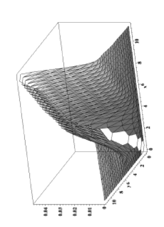
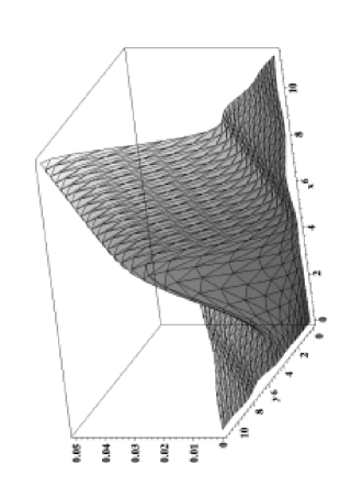
The dimensionless spectrum, based on equations (4.3.3) and (4.154), is

$${{\mathrm{d}}N\over{\mathrm{d}}x}=\frac{(n_{\mathrm{gas}}^{\mathrm{in}}-n_{\mathrm{gas}}^{\mathrm{out}})^{2}}{2\;n_{\mathrm{gas}}^{\mathrm{in}}n_{\mathrm{gas}}^{\mathrm{out}}}\int_{0}^{\infty}\left(\frac{n_{\mathrm{gas}}^{\mathrm{in}}\,x^{2}+n_{\mathrm{gas}}^{\mathrm{out}}\,y^{2}}{n_{\mathrm{gas}}^{\mathrm{in}}\,x+n_{\mathrm{gas}}^{\mathrm{out}}\,y}\right)^{2}D\left({x+y\over 2}\right){\sin^{2}(3[x-y]/4)\over(3[x-y]/4)^{2}}{\mathrm{d}}y,$$ (4.183)

where $n_{\mathrm{gas}}^{\mathrm{out}}(x)$ and $n_{\mathrm{gas}}^{\mathrm{in}}(y)$ are now the appropriate functions of $x$ and $y$ (See equations (4.176) and (4.175)). A factor $2$ has been manually inserted to account for the photon polarizations.

As a consistency check, the infinite volume limit is equivalent to making the formal replacements 

$${\sin^{2}(3[x-y]/4)\over(3[x-y]/4)^{2}}\to{4\pi\over 3}\delta(x-y),$$ (4.187)

and

$$D\left({x+y\over 2}\right)\to{1\over 2\pi^{2}}.$$ (4.188)

Doing so, equation (4.183) reduces to the spectrum obtained for homogeneous dielectrics in [17]. Indeed

$${{\mathrm{d}}N\over{\mathrm{d}}x}={1\over 3\pi}\frac{(n_{\mathrm{gas}}^{\mathrm{in}}-n_{\mathrm{gas}}^{\mathrm{out}})^{2}}{n_{\mathrm{gas}}^{\mathrm{in}}n_{\mathrm{gas}}^{\mathrm{out}}}\;x^{2}\;\Theta(x_{*}-x).$$ (4.189)

With these consistency checks out of the way, it is now possible to perform the integral with respect to $y$ to estimate the spectrum for finite volume, and similarly to perform appropriate double integrals with respect to $x$ and $y$ to estimate both total photon production and average photon energy. In the previous section we have seen that in the infinite volume limit there were two continuous branches of values for $n_{\mathrm{gas}}^{\mathrm{in}}$ and $n_{\mathrm{gas}}^{\mathrm{out}}$ that led to approximately one million emitted photons with an average photon energy of $3/4$ the cutoff energy. If we now place the same values of refractive index into the formula (4.183) derived above, numerical integration again yields approximately one million photons with an average photon energy of $3/4$ times the cutoff energy. The total number of photons is changed by at worst a few percent, while the average photon energy is almost unaffected. (Some specific sample values are reported in Table I.) The basic result is this: as expected, finite volume effects do not greatly modify the results estimated by using the infinite volume limit. Note that $\hbar\Omega_{\mathrm{max}}$ is approximately $4$ eV, so that average photon energy in this crude model is about $3$ eV.

$\;n_{\mathrm{gas}}^{\mathrm{in}}\;$	$\;n_{\mathrm{gas}}^{\mathrm{out}}\;$	Number of photons	$\langle E\rangle/\hbar\Omega_{\mathrm{max}}$
$2\times 10^{4}$	$1$	$1.06\times 10^{6}$	$0.803$
$71$	$25$	$1.00\times 10^{6}$	$0.750$
$68$	$34$	$1.06\times 10^{6}$	$0.751$
$9$	$25$	$0.955\times 10^{6}$	$0.750$
$1$	$12$	$0.98\times 10^{6}$	$0.765$

Table I: Some typical cases.

In addition, for the specific case $n_{\mathrm{gas}}^{\mathrm{in}}=2\times 10^{4}$, $n_{\mathrm{gas}}^{\mathrm{out}}=1$, we have calculated and plotted the form of the spectrum. We find that the major result of including finite volume effects is to smear out the otherwise sharp cutoff coming from Schwinger’s step-function model for the refractive index. Other choices of refractive index lead to qualitatively similar spectra. These results are in reasonable agreement (given the simplicity of the present model) with experimental data.

Figure 4.14: Spectrum ${\mathrm{d}}N/{\mathrm{d}}x$ obtained by integrating the approximated Bogoliubov coefficient. We integrate from $y=0$ to $y_{*}=11.5$ and plot the resulting spectrum from $x=0$ to $x=14.5$. For $n_{\mathrm{out}}=1$ and $R=500$nm the relation between the non-dimensional quantity $x$ and the frequency $\nu$ is $x\sim\nu\cdot 10.5\cdot 10^{-15}$s. So $x\approx 11.5$ corresponds to $\nu\approx 1.1$ PHz. The curve with the sharp cutoff is the infinite volume approximation. Finite volume effects tend to smear out the sharp discontinuity, but do not greatly affect the total number of photons emitted.

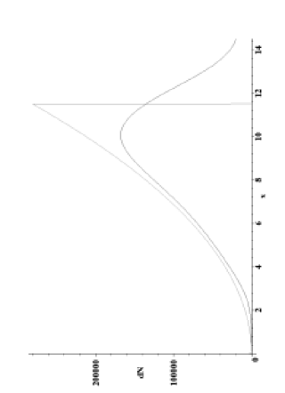
4.4 Experimental features and possible tests

Our proposal shares with other proposals based on the dynamical Casimir effect the main points of strength previously sketched. On the other hand it is important to stress that the above model implies a much more complex and rich collection of physical effects due to the fact that photon production from vacuum is no longer due to the simple motion of the bubble boundary. The model indicates that a viable Casimir route to SL cannot avoid a “fierce marriage” with features related to condensed matter physics. As a consequence our proposal is endowed both with general characteristics, coming from its Casimir nature, and with particular ones coming from the details underlying the sudden change in the refractive index.

Although the calculation presented above is just a “probe”, we can see that it is already able to make some general predictions that one can expect to see confirmed in a more complete approach. First of all the photon number spectrum the model predicts is not a black body. It is polynomial at low frequencies ($\omega^{2}$ in the infinite volume approximation we used), and in principle this difference can be experimentally detected. (The same qualitative prediction can be found in Schützhold et al. [245].) Moreover the spectrum is expected to be a power law dramatically ending at frequencies corresponding to the physical wave-number cutoff $K$ (at which the refractive indices go to 1). This cutoff implies the absence of hard UV photons and hence, in accordance with experiments, the absence of dissociation phenomena in the water surrounding the bubble.

In this type of model, the flash of photons is predicted to occur at the end of the collapse, the scale of emission zone is of the order of $500\;\hbox{nm}$, and the timescale of emission is very short, with a rise-time of the order of femtoseconds, though the flash duration may conceivably be somewhat longer . These are points in substantial agreement with observations. In the infinite volume limit the photons emerge in strictly back-to-back fashion. In contrast, for a finite volume bubble we have seen that the size of the emitting region constrains the model to low angular momentum for the out states. This is a very sharp prediction that is in principle testable with a suitable experiment devoted to the study of the angular momentum decomposition of the outgoing radiation.

Regarding other experimental dependencies, such as the temperature of the water or the role of noble gases, we can give general arguments but a truly predictive analysis can be done only after focusing on a specific mechanism for changing the refractive index.

For instance, the presence of noble gas is likely to change solubilities of gas in the bubble, and this can vary both bubble dynamics and the sharpness of the boundary. Alternatively, a small percentage of noble gas in air can be very important in the behavior of its dielectric constant at high pressure. Indeed, while small admixtures of noble gas will not significantly alter the zero-frequency refractive index, from the Casimir point of view the behaviour of the refractive index over the entire frequency range up to the cutoff is important.

Finally, the temperature of water can instead affect the dynamics of the bubble boundary by influencing the stability of the bubble, changing either the solubility of air in water or the surface tension of the latter. As observed by Schwinger, temperature can also affect the dielectric cutoff, and so temperature dependence of SL is quite natural in Schwinger-like approaches.

The above discussion should make clear that an actual experimental test of the proposed explanation of Sonoluminescence would require as an unavoidable precondition a much more detailed understanding of the dynamics of the refractive indices of the gas and of the surrounding water. Nevertheless one may wonder if a general signature of the quantum particle creation from the vacuum can be found.

As we said the quasi-thermal nature of the emitted photons can be explained by the squeezed nature of the photon pairs that are generically created via the dynamical Casimir effect. In this case the core of the bubble is not required to achieve the tremendous physical temperatures envisaged by other models.

We have seen in chapter 1 how this apparent thermality can emerge, in what follow we shall try to investigate this aspect of the photon emission for our specific models and to find an univocal signature of the squeezed nature of the photons pair produced by an eventual dynamical Casimir effect.

4.4.1 Squeezed states as a test of Sonoluminescence

From what we said, thermal characteristics in single photon measurements in Sonoluminescence can be associated with at least two hypotheses: (a) real physical thermalization of the photon environment; (b) pseudo-thermal single photon statistics due to tracing over the unobserved member of a photon pair that is actually produced in a two-mode squeezed state. We shall call case (a) real thermality; while case (b) will be denoted effective thermality. Of course, case (b) has no relation with any concept of thermodynamic temperature, though to any such squeezed state one may assign a (possibly mode-dependent) effective temperature.

Our aim is to find a class of measurements able to discriminate between cases (a) and (b), and to understand the origin of the roughly thermal spectrum for Sonoluminescence in the visible frequency range. In principle, the thermal character of the experimental spectrum could disappear at higher frequencies, but for such frequencies the water medium is opaque, and it is not clear how we could detect them. (Except through heating effects.)

To treat Sonoluminescence, we introduce a quantum field theory characterized by an infinite set of bosonic oscillators (as in bosonic Thermofield Dynamics; not just two oscillators as in the case of “signal-idler” systems studied in quantum optics). The simple two-mode squeezed vacuum discussed in section 1.3.3 is then replaced by

$$|\Omega[\zeta(k,k^{\prime})]\rangle\equiv\exp\left[-\int{\mathrm{d}}^{3}k\;{\mathrm{d}}^{3}k^{\prime}\;\zeta(k,k^{\prime})\left(a_{k}b_{k^{\prime}}-a^{\dagger}_{k}b^{\dagger}_{k^{\prime}}\right)\right]|0\rangle,$$ (4.190)

where the function $\zeta(k,k^{\prime})$ is peaked near $k+k^{\prime}=0$, and becomes proportional to a delta function in the case of infinite volume [$\zeta(k,k^{\prime})\to\zeta(k)\delta(k+k^{\prime})$] when the photons are emitted strictly back-to-back. To be concrete, let us refer to the homogeneous dielectric model presented in Sec. 4.2. In this limit there is no “mixing” and everything reduces to a sum of two-mode squeezed-states, where each pair of back-to-back modes is decoupled from the other. The frequency $\omega$ is the same for each photon in the couple, in such a way that we are sure to get the same “temperature” for both. The two-mode squeezed vacuum then simplifies to

$$|\Omega(\zeta_{k})\rangle\equiv\exp\left[-\int{\mathrm{d}}^{3}k\ \zeta_{k}\left(a_{k}a_{-k}-a^{\dagger}_{k}a^{\dagger}_{-k}\right)\right]|0\rangle.$$ (4.191)

It is interesting to note that, if photons are pair produced in two-mode squeezed-states by a suitable pair production interaction term, then $T_{\mathrm{squeezing}}$ is a function of both frequency and squeezing parameter, and in general only a special “fine tuning” would allow us to get the same effective temperature for all couples. If we consider the expectation value on the state $|\Omega(\zeta_{k})\rangle$ of $N_{k}\equiv a^{\dagger}_{k}a_{k}$ we get

$$\langle\Omega(\zeta_{k})|N_{k}|\Omega(\zeta_{k})\rangle=\sinh^{2}(\zeta_{k}),$$ (4.192)

so we again find a “thermal” distribution for each value of $k$ with temperature

$$k_{\rm B}T_{k}\equiv\frac{\hbar\omega_{k}}{2\;\log(\coth(\zeta_{k}))}.$$ (4.193)

The point is that for $k\neq{\bar{k}}$ we generally get $T_{k}\neq T_{\bar{k}}$ unless a fine tuning condition holds. This condition is implicitly made in the definition of the thermofield vacuum and it is possible only if we have

$$\coth(\zeta_{k})=\hbox{e}^{\kappa\omega_{k}},$$ (4.194)

with $\kappa$ some constant, so that the frequency dependence in $T_{k}$ is canceled and the same $T_{\rm squeezing}$ is obtained for all couples.

For models of Sonoluminescence based on the dynamical Casimir effect (i.e. squeezing the QED vacuum) we cannot rely on a definition to provide the fine tuning, but must perform an actual calculation. The model of Sec. 4.2 is again a useful tool for a quantitative analysis. We have (omitting indices for notational simplicity; our Bogoliubov transformation is diagonal) the following relation between the squeezing parameter and the Bogoliubov coefficient $\beta$

$$\langle N\rangle=\sinh^{2}(\zeta)=|\beta|^{2},$$ (4.195)

where, by defining $\varphi\equiv\pi\;t_{0}/({\textstyle n_{\mathrm{in}}^{2}+n_{\mathrm{out}}^{2}})$, (here $t_{0}$ is the timescale on which the refractive index changes) one has from Eq. (4.40)

$$|\beta|^{2} \propto {\sinh^{2}\left({\textstyle|n_{\mathrm{in}}^{2}\omega_{\mathrm{in}}-n_{\mathrm{out}}^{2}\omega_{\mathrm{out}}|}\;\varphi\right)\over\sinh\left(2\;{\textstyle n_{\mathrm{in}}^{2}}\;\omega_{\mathrm{in}}\varphi\right)\;\sinh\left(2\;{\textstyle n_{\mathrm{out}}^{2}}\;\omega_{\mathrm{out}}\varphi\right)}.$$ (4.196)

In the adiabatic limit (large frequencies) we get a Boltzmann factor (4.54)

$$|\beta|^{2}\approx\exp\left(-4\;\hbox{min}\{n_{\mathrm{in}},n_{\mathrm{out}}\}n_{\mathrm{out}}\;\omega_{\mathrm{out}}\varphi\right).$$ (4.197)

Since $|\beta|$ is small, $\sinh(\zeta)\approx\tanh(\zeta)$, so that in this adiabatic limit

$$|\tanh(\zeta)|^{2}\approx\exp\left(-4\;\hbox{min}\{n_{\mathrm{in}},n_{\mathrm{out}}\}n_{\mathrm{out}}\;\omega_{\mathrm{out}}\varphi\right),$$ (4.198)

$$k_{\rm B}T_{\mathrm{effective}}\approx\frac{\hbar}{8\pi t_{0}}\,\frac{n_{\mathrm{in}}^{2}+n_{\mathrm{out}}^{2}}{n_{\mathrm{out}}\hbox{min}\{n_{\mathrm{in}},n_{\mathrm{out}}\}}$$ (4.199)

Thus for the entire adiabatic region we can assign a single frequency-independent effective temperature which is really a measure of the speed with which the refractive index changes. Physically, in Sonoluminescence this observation applies only to the high-frequency tail of the photon spectrum.

In contrast, in the low frequency region, where the bulk of the photons emitted in Sonoluminescence are to be found, the sudden approximation holds and the spectrum is phase space limited (a power law spectrum), not Planckian. It is nevertheless still possible to assign a different effective temperature for each frequency.

Finite volume effects smear the momentum space delta function so we no longer get exactly back-to-back photons. This represents a further problem because we have to return to the general squeezed vacuum of equation (4.190). It is still true that photons are emitted in pairs, pairs that are now approximately back-to-back and of approximately equal frequency. We can again define an effective temperature for each photon in the couple as in the “signal-idler” systems of quantum optics. Such temperature is no longer the same for the two photons belonging to the same couple and no “special condition” for getting the same temperature for all the couples exists. We have seen how analyzing these finite volume distortions is not easy.

In summary: The photons produced in a dynamical Casimir effect are not truly thermal but can be cast in the framework of “effective thermality”. The spectrum is Planckian or not depending on whether the adiabatic regime or sudden regime holds sway, but even in the sudden regime a frequency-dependent effective temperature can be assigned to each photon mode. Finite volume effects are difficult to deal with quantitatively, but the qualitative result that in any dynamic Casimir effect model of Sonoluminescence there should be strong correlations between approximately back-to-back photons is robust. It is this last observation that leads us to the following proposal.

Two photon observables

Define the observable

$$N_{ab}\equiv N_{a}-N_{b},$$ (4.200)

and its variance

$$\Delta(N_{ab})^{2}=\Delta N_{a}^{2}+\Delta N_{b}^{2}-2\langle N_{a}N_{b}\rangle+2\langle N_{a}\rangle\langle N_{b}\rangle.$$ (4.201)

These number operators $N_{a},N_{b}$ are intended to be relative to photons measured, e.g., back to back photons. In the case of true thermal light we get

$$\Delta N_{a}^{2}=\langle N_{a}\rangle(\langle N_{a}\rangle+1),$$ (4.202)

$$\langle N_{a}N_{b}\rangle=\langle N_{a}\rangle\langle N_{b}\rangle,$$ (4.203)

so that

$$\Delta(N_{ab})^{2}_{\mathrm{thermal\ light}}=\langle N_{a}\rangle(\langle N_{a}\rangle+1)+\langle N_{b}\rangle(\langle N_{b}\rangle+1).$$ (4.204)

For a two-mode squeezed-state

$$\Delta(N_{ab})^{2}_{\mathrm{two\ mode\ squeezed\ light}}=0.$$ (4.205)

Due to correlations, $\langle N_{a}N_{b}\rangle\neq\langle N_{a}\rangle\langle N_{b}\rangle$. Note also, that if you measure only a single photon in the couple, you get (as expected) a thermal variance $\Delta N_{a}^{2}=\langle N_{a}\rangle(\langle N_{a}\rangle+1)$. Therefore a measurement of the variance $\Delta(N_{ab})^{2}$ can be decisive in discriminating if the photons are really thermal or if nonclassical correlations between the photons occur [56]. If the “thermality” in the Sonoluminescence spectrum is of this squeezed-mode type, one will ultimately desire a more detailed model of the dynamical Casimir effect involving an interaction term that produces pairs of photons in two-mode squeezed-states.

4.5 Discussion and Conclusions

We have verified by explicit computation that photons are produced by rapid changes in the refractive index, and are in principle able to explain the observed photons of Sonoluminescence.

Based largely on the fact that efficient photon production requires timescales of the order of femtoseconds, we were led to consider rapid changes in the refractive index as the gas bubble bounces off the van der Waals hard core. It is important to realize that the speed of sound in the gas bubble can become relativistic at this stage.

A key lesson learned from this investigation is that in order for the conversion of zero-point fluctuations to real photons to be relevant for Sonoluminescence, we would want the sudden approximation to hold for photons all the way out to the cutoff ($200\;\hbox{nm}$; corresponding to a period of $0.66\times 10^{-15}\;\hbox{seconds}$), a femtosecond timescale. This implies that if conversion of zero-point fluctuations to real photons is a significant part of the physics of Sonoluminescence then the refractive index must be changing significantly on femtosecond timescales. Thus the changes in refractive index cannot be only due to the motion of the bubble wall. (The bubble wall is moving at most at Mach 4 [216]; for a $1\;\mu\hbox{m}$ bubble this gives a collapse timescale of $10^{-10}$ seconds, about 100 picoseconds.)

We have thus suggested that one should not be focusing on the actual collapse of the bubble, but rather on the way in which the refractive index changes as a function of space and time. As the bubble collapses the gases inside are compressed, and although the refractive index for air (plus noble gas contaminants) is 1 at STP it should be no surprise to see the refractive index of the trapped gas undergoing major changes during the collapse process — especially near the moment of maximum compression when the molecules in the gas bounce off the van der Waals’ hard core repulsive potential.

Thus attempts at using the dynamical Casimir effect to explain SL are now much more tightly constrained than previously. We have shown that any plausible model using the dynamical Casimir effect to explain SL must use the sudden approximation, and must have very rapid changes in the refractive index. Our model shows that this timescale is a non-trivial function of the sudden approximation cut-off frequency, $\Omega_{\rm sudden}$, and of the initial and final values of the refractive index $(n_{\mathrm{in}},n_{\mathrm{out}})$. For this reason a million photons can be obtained for values of the typical timescale up to some picoseconds.

A complete theory of SL will need to address much more specific timing information and this will require a fully dynamical approach (from the QFT point of view) and a deeper understanding (from the condensed matter side) of the precise spatio-temporal dependence of the refractive index as the bubble collapses. Moreover also theoretically our model could be improved by taking into account a multicycle process. In this case the periodicity in the change of the refractive index should lead to a parametric-resonance behaviour. Such sorts of regime are very important (as we shall see) in the discussion of the preheating phase in inflationary scenarios. In analogy, a parametric resonance regime could greatly improve the efficiency of the production of photons.

In the absence of such a more detailed description, the present calculation is a useful first step. Moreover it allows us to specify certain basic “signatures” of the effect that may be amenable to experimental test.

We have proposed the possibility of discriminating between real thermal photons and dynamical Casimir photons by means of a careful analysis of two-photon correlation statistics. Let us start by making the ansatz that thermality in the spectrum is either real or “effective” in the sense described above. In the former case, adiabatic heating models are not compatible with some recent experimental data showing that there is no time delay between different emitted frequencies [217, 218]. However there remains the possibility for nonadiabatic heating (Bremsstrahlung or shock wave models). For thermal light one should find thermal variance for photon pairs. On the other hand, thermofield-like photons should show zero variance in appropriate pair correlations. So we propose to not deal directly with the issue of thermality by looking at the spectrum, on the contrary we propose to deal with correlations of photons approximately emitted back to back.

In conclusion we believe that the present calculation (limited though it may be) represents an important advance: there can now be no doubt that changes in the refractive index of the gas inside the bubble lead to the production of real photons — the controversial issues now move to quantitative ones of precise fitting of the observed experimental data. Casimir models are now driven into a relatively small region of parameter space, and one can be hopeful of having experimental verification (or falsification) of them in the not too distant future.

Chapter 5 Quantum vacuum effects in the early universe

As a working hypothesis to explain the riddle of our existence,

I propose that our universe is the most interesting of all possible universes,

and our fate as human beings is to make it so.

Freeman Dyson

In this chapter we shall deal with some quantum vacuum effects in the very early universe. After discussing the influence of the topological Casimir effect in cosmology, we shall review the inflationary paradigm, paying particular attention to the theory of preheating via parametric resonance. In this framework we shall propose a new channel of particle creation which we shall call “geometric preheating”. We shall show that this effect can lead to the production of extremely heavy particles as required by baryogenesis theory. After this investigation we shall consider the possibility of developing an alternative scenario to inflation for solving the cosmological puzzles. In particular we shall focus our attention on the recently proposed variable speed of light cosmologies (VSL). A critical discussion concerning the foundations of such scenarios will lead us to propose a new class of such models, the $\chi$–Variable–Speed–of–Light cosmologies. Their value as possible alternatives to inflation or as a “partner” for this, nowadays standard, framework, will be investigated in detail.

5.1 The role of the quantum vacuum in modern cosmology

Although theoretical speculation about the meaning and the structure of the universe has characterized almost all of the civilizations which have appeared on earth it is nevertheless true that cosmology has become a true science only with the advent of General Relativity. It is true, in fact, that it is just with the full understanding of the Einstein equations that the basis for the development of predictive cosmological models arose.

A quite outstanding fact of this research is that it has led to a dramatic revolution in our understanding of the place that we have in the universe and to the final realization that the “cosmos” is not a never-changing place, quiet and peaceful. It appears to us instead as a dynamical ensemble of matter and energy, a place where huge forces are in action and can finally lead to unexpected results.

Among the “surprises” which General Relativity had in store for us, mention should be made of the discovery of space-time singularities. In the particular case of cosmology it was realized that singularities are unavoidable in General Relativity if matter satisfies some of the energy conditions which we discussed in chapter 1. The realization that quantum vacuum effects in strong fields generally violate most of these energy conditions, soon led to a great interest in the application of these effects to cosmology and now this has grown into a well-established branch of research.

The quantum vacuum can influence cosmological models in two general ways. The renormalized SET can be such as to strongly modify the evolution of the universe (via the semiclassical Einstein equations). Alternatively one can have situations in which the vacuum effects are manifested via dynamical particle production; in these cases the gravitational field or a matter field drives the emission of quanta of some quantum fields, sometimes with relevant effects for the late-time appearance of the universe.

Two typical examples for the first class of phenomena are the topological Casimir effect and the inflationary phase of an FLRW universe. The second class has instead its major realizations in the generation of perturbations in the inflationary framework and in the theory of formation and evaporation of primordial black holes.

We shall not study in detail this second class of phenomena although we shall discuss the role of the quantum vacuum in the production of the primordial spectrum of perturbations. Regarding primordial black holes, they may affect the outcome of Big Bang nucleosynthesis [254] and be of astrophysical interest through their evaporative production of very high energy cosmic rays [255] and as promising candidates for explaining the Massive Compact Halo Objects (MACHOs) detected in the halo of our galaxy (these objects would have masses of about $0.2$ to $0.8$ $M_{\odot}$) [256]. Also, considerations of the possible formation of primordial black holes during cosmic phase transitions (e.g., the electroweak and quantum chromodynamic (QCD) transitions) may be helpful for improving our understanding of the related particle physics.

In the following we shall concentrate our attention on the topological Casimir effect in cosmology and its possible role in the evolution of our universe.

5.2 The topology of the universe and the quantum vacuum

The information which we can get about a cosmological solution by using the Einstein equations is not complete. In fact these are partial differential equations and are hence able to describe just the local properties of spacetime. These properties are indeed completely encoded in the infinitesimal distance element ${\mathrm{d}}s^{2}=g_{\mu\nu}{\mathrm{d}}x^{\mu}{\mathrm{d}}x^{\nu}$.

The global structure — the topology — of the spacetime is instead out of the domain of the Einstein equations, actually several distinct topologies can be associated with the same local metric element. This realization has important consequences for modern cosmology.

According to the standard cosmological framework, the requirement of spatial homogeneity and isotropy has led to the so-called Friedmann-Lemaître-Robertson-Walker metrics

$${\mathrm{d}}s^{2} = -c^{2}\;{\mathrm{d}}t^{2}+a^{2}(t)\;h_{ij}\;{\mathrm{d}}x^{i}\;{\mathrm{d}}x^{j},$$ (5.1)

$$h_{ij}{\mathrm{d}}x^{i}{\mathrm{d}}x^{j} = \frac{{\mathrm{d}}r^{2}}{1-Kr^{2}}+r^{2}\left({\mathrm{d}}\theta^{2}+\sin^{2}\theta{\mathrm{d}}\varphi^{2}\right)$$

where $K=0,\pm 1$ denotes the space curvature. For generic $a(t)$, the above metric describes Friedmann models; for $a(t)$ described by hyperbolic laws we get the maximally symmetric de Sitter solution, an exponentially expanding 3-space. More precisely one gets

$$a(t)=H^{-1}\cosh(Ht)\qquad\mbox{for}\quad K=+1$$ (5.2)

$$a(t)=a_{0}\exp(Ht)\qquad\quad\,\,\mbox{for}\quad K=0$$ (5.3)

$$a(t)=H^{-1}\sinh(Ht)\qquad\mbox{for}\quad K=-1$$ (5.4)

where $H=\dot{a}/a$ is the Hubble parameter and $a_{0}$ is the value of $a(t)$ at $t=0$. In dealing with FLRW models it is generally assumed that the global structure of space is that of the infinite Euclidean space $R^{3}$, or that of the finite hypersphere $S^{3}$ or that of the infinite hyperbolic space $H^{3}$. The choice depends on whether the constant spatial curvature is respectively zero, positive or negative ($K=0,\pm 1$).

The above considerations instead lead to the possibility that the above spatial topologies are not the only ones compatible with the FLRW metric. Indeed a large number of topologies obtained from the former ones by opportune identifications of some set of points, are compatible with (5.1). The standard spatial topologies associated with $R^{3}$, $S^{3}$ and $H^{3}$ describe simply connected manifolds, that is manifolds for which, at any point ${\mathbf{x}}$, a loop can be continuously shrunk to a point. The identifications of some points of these manifolds leads to their corresponding “non-simply connected” or “multiply-connected” versions. In particular, this implies that even for zero or negative spatial curvatures, the FLRW models could nevertheless correspond to compact space topologies. For spaces of constant curvature (such as the FLRW models) these compact manifolds can be expressed as the quotient ${\cal M}\equiv\tilde{\cal M}/{\Gamma}$ where $\tilde{\cal M}$ is one of the three simply connected topologies mentioned above and $\Gamma$ is a subgroup of isometries of $\tilde{\cal M}$ acting freely and discontinuously ($\Gamma$ can also be interpreted as the holonomy group in $\tilde{\cal M}$, see [257] for an extensive review of these issues).

Although some important work has been done in the last few decades on the possibility that the topology of our universe could be non-simply connected, cosmologists have often ignored this important possibility which is moreover apparently favoured by quantum cosmology predictions (see for example [258, 259]).

For what concerns the spirit of our research, the possibility of having non-trivial topologies for the spatial sections of FLRW spacetimes can certainly be considered as being among the most promising testing fields for the theory of quantum vacuum effects in strong fields.

We have seen in chapter 1 how the non-trivial topology of flat space can lead to a vacuum polarization, a topological Casimir effect. In cosmological models with non simply connected spaces, the same sort of effects can be expected and indeed predicted [126, 127, 128]. In these cases the Casimir effect will be calculated using as the reference vacuum state — with respect to which the Casimir subtraction is performed — the appropriate one in the simply connected manifold ${\cal M}$.

In this way it is possible to obtain a finite Casimir contribution to the total quantum field vacuum SET, $\langle T_{\mu\nu}\rangle_{\mathrm{tot}}$, and hence a semiclassical backreaction effect on the spacetime metric, via the semiclassical Einstein equations:

$$G_{\mu\nu}+\Lambda g_{\mu\nu}=8\pi G_{\mathrm{N}}\langle T_{\mu\nu}\rangle_{\mathrm{tot}}$$ (5.5)

We note that this is indeed a nice example of how the global configuration can influence the local structure of the universe via the quantum vacuum.

In connection with the problem of backreaction, particular attention should be devoted to the so-called self-consistent models of the universe. These are cosmological solutions which do not contain any classical matter field but are instead completely governed by vacuum quantum effects. Consistency is achieved when the SET for a given class of metrics gives a metric of the same form if it is re-inserted into the semiclassical Einstein equations (5.5).

Comment: Self-consistency is not generic. This can be understood from the simple fact that even the choice between periodic and anti-periodic conditions on the quantized fields, can lead to different signs for the renormalized SET. Moreover in [126] it is shown that the tensorial structure of the SET obtained by the topological Casimir effect in Clifford-Klein spaces of the form $\tilde{\cal M}=S^{3}/\Gamma$ is generally different from that of the Einstein tensor $G_{\mu\nu}=R_{\mu\nu}-g_{\mu\nu}R/2$ because the former contains additional geometrical structure. It is perhaps conceivable to impose constraints on the admitted non-simply connected realizations of FLRW cosmologies exactly by looking at the compatibility of the tensorial structure of the renormalized SET with the Einstein equations.

As an example of a self-consistent model we can consider the topological Casimir effect associated with a non-simply connected version of the flat FLRW cosmological model, taking $\tilde{\cal M}=R^{3}/\Gamma$ and $K=0$ in Eq. (5.1). For our purposes is convenient to use Cartesian coordinates $(t,x,y,z)$, and the metric element (5.1) is then

$${\mathrm{d}}s^{2}=-{\mathrm{d}}t^{2}+a^{2}(t)\left({\mathrm{d}}x^{2}+{\mathrm{d}}y^{2}+{\mathrm{d}}z^{2}\right)$$ (5.6)

All of the possible non-simply connected versions of such a space have been described by Wolf  [129] and there are 18 variants (including the simply connected topology $R^{3}$).

We shall now focus on the very simple case in which the space sections have a toroidal topology of characteristic length $L$. This topological structure corresponds to some natural periodic conditions

$$\left\{\begin{array}[]{lll}x&=&x+kL\\ y&=&y+mL\\ z&=&z+nL\end{array}\right.\qquad k,m,n=\pm 1,\pm 2,\dots$$ (5.7)

In this model, the three-dimensional volume of the universe is always finite and is given by $V=a^{3}(t)L^{3}$.

The topological Casimir effect in compact three-dimensional spaces with flat geometry is a somewhat trivial generalization of the one-dimensional example discussed in chapter 1. In particular, the renormalized energy density for a massless scalar field in a torus with typical scales $b,c,d$ can be shown to be [6]

$$\epsilon=-\frac{\pi^{2}}{90b^{4}}-\frac{\zeta(3)}{2\pi bc^{3}}-\frac{\pi}{6bcd^{2}}$$ (5.8)

where $\zeta$ is the so called Riemann $\zeta$-function and $\zeta(3)\approx 1.202$. We stress that we have here lost the symmetry under permutations of $a$, $b$ and $c$ because some terms are dropped making the assumption $b\leq c\leq d$.

The pressures along the spatial axes can also be obtained by using their relation with the total energy $E=bcd\epsilon$ say

$$P_{x}=-\frac{1}{cd}\frac{\partial E}{\partial b}\quad P_{y}=-\frac{1}{db}\frac{\partial E}{\partial c}\quad P_{z}=-\frac{1}{bc}\frac{\partial E}{\partial d}\quad$$ (5.9)

In our case $b=c=d=a(t)L$ and so the Casimir SET for a massless, conformally coupled field, takes the form (taking into account the terms previously ignored in Eq.(5.8)) [6]

$$\langle T^{0}_{0}\rangle=-\frac{0.8375}{a^{4}(t)L^{4}},\quad\langle T^{i}_{i}\rangle=-\frac{1}{3}\langle T^{0}_{0}\rangle$$ (5.10)

The inclusion of fields with anti-periodic conditions changes, in this case, just the numerical coefficient in the above formula [6] and for generality we can replace the $0.8375$ by a positive constant $A$. Inserting now the above SET in the Einstein equations (5.5) for the flat FLRW metric, one gets

$$3\dot{a}^{2}-\Lambda a^{2}=-\frac{8\pi G_{\mathrm{N}}A}{a^{2}L^{4}}$$ (5.11)

which admits the solution [260]

$$a(t)=\frac{1}{L}\left(\frac{8\pi G_{\mathrm{N}}A}{\Lambda}\right)^{1/4}\left[\cosh\left(2\sqrt{\frac{\Lambda}{3}t}\right)\right]^{1/2}$$ (5.12)

This implies that, for the case being considered, the topological Casimir SET induced by the compactification of flat $R^{3}$ spatial sections leads to a non-singular universe with accelerated expansion, a de Sitter spacetime. This was the sort of solution to be expected just because of the presence of a non-zero cosmological constant $\Lambda$ and hence the result is a nice example of a self-consistent model .

The property of de Sitter spacetime which we have just found is a good starting point for our next topic. In fact this spacetime has some other peculiar characteristics which play a crucial role in modern cosmology.

5.3 Inflation

As we said at the start of this chapter, modern cosmology is based on the equations of General Relativity and on the Copernican principle of isotropy and homogeneity of our universe. The SET of matter is assumed to be that of a perfect fluid .

$$T^{\mu\nu}=\left[\matrix{\rho c^{2}&0&0&0\cr 0&p&0&0\cr 0&0&p&0\cr 0&0&0&p}\right].$$ (5.13)

where $\rho$ and $p$ are respectively the total density and the total pressure of all of the different kinds of matter considered in the model.

By these basic elements, it is straightforward to arrive at the FLRW cosmologies. These are characterized by the class of metrics determined by (5.1) and are governed by the so-called Friedmann equations

$${\left({\dot{a}\over a}\right)}^{2} = {8\pi G_{\mathrm{N}}\over 3}\;\rho-{{Kc^{2}}\over a^{2}}+\frac{\Lambda c^{2}}{3},$$ (5.14)

$${\ddot{a}\over a} = -{4\pi G_{\mathrm{N}}\over{3c^{2}}}\;\left(\varepsilon+3p\right).$$ (5.15)

where, again, $K=0,\pm 1$.

This framework nowadays takes the name of “the standard model of cosmology” (SM), and the wide consensus which it has managed to obtain in the scientific community is based mainly on three confirmed experimental predictions:

1. The Hubble law

2. The Cosmic Microwave Background Radiation (CMBR)

3. The abundances of light elements

The third observation, which is a direct test of the more general nucleosynthesis theory, represents the earliest-time probe of the SM to have been developed so far. In fact, the light element production is supposed to have taken place between a second and a few minutes after the Big Bang (the initial singularity predicted by the Hawking–Penrose theorem which we cited in chapter 1). For times between that one and the Planck time $t_{\mathrm{Pl}}=10^{-44}s$ (where quantum gravity should come onto the stage) we have no direct proof of the validity of the SM. It is exactly from this “no-man’s land” that the main trouble for the standard model arises.

5.3.1 The cosmological Puzzles

In spite of its remarkable success, the SM has proved to be unable to explain some striking observational features of our universe. All of these features seem to have an extremely remote origin (before the first second after the Big Bang).

These “failures” of the standard model are generally called the “cosmological puzzles”. These are substantially things that the framework is unable to justify and about which it cannot give to us any satisfactory response without appealing to very special initial conditions for the cosmological evolution. Here we shall limit ourselves to a rapid survey of these puzzles, directing the reader to standard cosmology textbooks for further information.

The horizon problem

The CMBR is isotropic to $1$ part in $10^{5}$ (after excluding the dipole due to our peculiar velocity). The horizon problem arises from the fact that regions at the antipodes of our horizon have never had the chance to get in causal contact according to the SM. More concretely, one finds that the particle horizon at the time of photon decoupling (redshift $z\approx 1200$) subtends just one degree in the sky and so, at the time when the photons were emitted, two nowadays antipodal points were separated by very many particle horizons of that time and were hence causally disconnected. How then is it possible that regions which had never exchanged information appear to be at the same temperature with such high precision?

Comment: We would like to make clear a point related to the definition of horizons in cosmology. Speaking about regions in causal contact, the pertinent horizon which one should consider is the so-called particle horizon $$\ell_{\mathrm{h}}(t)=a(t)\int_{0}^{t}{\frac{c\,{\mathrm{d}}t^{{}^{\prime}}}{a(t^{{}^{\prime}})}}$$ (5.16) This is telling us the distance covered by light in a time $t$ and hence the largest region which can be in causal contact at that time. As clearly explained in [261], this quantity should not be confused with the length scale given by $$R_{\mathrm{H}}={c\over H}.$$ (5.17) The above quantity (known as the Hubble radius) is often mistakenly confused with the particle horizon. The Hubble scale evolves in the same way as the particle horizon in simple FLRW models and hence measures the domain of future influence of an event in these models [262]. If fields interact only through gravity, then the Hubble scale is useful as a measure of the minimum spatial wavelength of those modes that are effectively “frozen in” by the expansion of the universe. A mode is said to be “frozen in” if its frequency is smaller than the Hubble parameter, since then there is not enough time for it to oscillate before the universe changes substantially and so the evolution of that mode is governed by the expansion of the universe. Therefore, for modes traveling at the speed $c$, if the “freeze out” occurs at $\omega<H$, this implies that $\lambda>c/H$, as claimed above. So while the particle horizon is truly the extension of a region potentially causally connected via microphysics, the Hubble scale has more the meaning of a “dynamical” scale. This is not surprising if one realizes that the Hubble time $H^{-1}\approx 1/\sqrt{G_{\mathrm{N}}\rho}$ is exactly the dynamical time which characterizes all of the gravitational phenomena.

As a final remark it is useful to stress that, even if regions at the antipodes of our universe would have somehow been in causal contact, this is still just a necessary, but not sufficient, condition in order to get isotropization. As shown in [263], the solutions which achieve a permanent isotropization represent a subset of measure zero in the set of all possible SM solutions.

The flatness problem

The standard model predicts that the universe can be flat, closed or open depending on its content of matter. The Friedmann equations show that there is a critical value for the mass density, which determines which regime the universe is in. Actually, imposing $\Lambda=K=0$ in Eq. (5.14), one finds that an FLRW model admits Euclidean spatial sections if

$$\rho_{{\mathrm{c}}}=\frac{3H^{2}}{8\pi G_{\mathrm{N}}}$$ (5.18)

Current observations seem to indicate that the ratio between the present density $\rho_{0}$ and the critical one is $\Omega_{0}=\rho_{0}/\rho_{{\mathrm{c}}}\approx 1$. More precisely the observations bound $\Omega_{0}$ in the range $[0.1,1]$.

The flatness problem arises from the fact that in FLRW cosmologies the solutions with $\Omega\approx 1$ are not at all attractors. On the contrary they represent unstable solutions given the fact that $\Omega(t)\to 0$ or $\infty$ in time.

The entropy problem

It is interesting to note that (at least in the usual framework) the two major cosmological puzzles described above (isotropy/horizon and flatness) can be reduced to a single problem related to the huge total amount of entropy that our universe appears to have today [264, 265, 266]. If we define $s\propto T^{3}$ the entropy density associated with relativistic particles and $S=a^{3}(t)s$ the total entropy per comoving volume, then it is easy to see from the Friedmann equation (5.108) that

$$a^{2}=\frac{Kc_{\mathrm{gravity}}^{2}}{H^{2}(\Omega-1)},$$ (5.19)

and so

$$S=\left[\frac{Kc_{\mathrm{gravity}}^{2}}{H^{2}\left(\Omega-1\right)}\right]^{3/2}s.$$ (5.20)

The value of the total entropy can be evaluated at the present time and comes out to be $S>10^{87}$. One can then see that explaining why $\Omega\approx 1$ (the flatness problem) is equivalent to explaining why the entropy of our universe is so huge.

In a similar way one can argue (at least in the usual framework) that the horizon problem can be related to the entropy problem [264, 265, 266]. In order to see how large the causally connected region of the universe was at the time of decoupling with respect to our present horizon, we can compare the particle horizon at time $t$ for a signal emitted at $t=0$, $\ell_{\mathrm{h}}(t)$, with the radius at same time, $L(t)$, of the region which now corresponds to our observed universe of radius $L_{\mathrm{present}}$. The fact that (assuming insignificant entropy production between decoupling and the present epoch) $(\ell_{\mathrm{h}}/L)^{3}|_{t_{\mathrm{decoupling}}}\ll 1$ is argued to be equivalent to the horizon problem.

Once again, a mechanism able to greatly increase $S$ via a non-adiabatic evolution would also automatically lead to the resolution of the puzzle.

The monopole problem

Another interesting problem arises when one tries to take into account particle physics knowledge within the SM framework. It is in fact a general prediction of Grand Unified Theories (GUTs) — the set of theories that try to unify the electro-weak and strong interaction — that monopoles should form as a consequence of the $SU(2)$ subgroup structure inherited from electroweak interactions. These monopoles are topologically stable knots in the Higgs field expectation value and are expected to have masses of order $m_{\mathrm{m}}\approx 10^{16}GeV$.

In particular, the Kibble mechanism [267] predicts a number density of topological defects $n_{\mathrm{m}}$ which is inversely proportional to the third power of the correlation length $\xi$ of the Higgs field

$$n_{\mathrm{m}}\approx{1\over\xi^{3}}$$ (5.21)

In the standard model the natural upper bound for the monopole density is given by the particle horizon at the moment of their formation. In fact causality constrains the correlation length of the Higgs field to be less that the particle horizon $\ell_{\mathrm{h}}$. In GUTs, the phase transition which generates these monopoles is generally predicted to occur at $T_{\mathrm{GUT}}\approx 10^{14}GeV$ and this temperature is achieved at approximately $t_{\mathrm{GUT}}\approx 10^{-35}s$ after the big bang. In standard cosmology, one has that in the radiation dominated era $a(t)\propto\sqrt{t}$ so $\ell_{\mathrm{h}}=2t$ and so

$$n_{\mathrm{m}}\approx{1\over\xi^{3}}\geq\frac{1}{8t^{3}_{\mathrm{GUT}}}$$ (5.22)

From the fact that the monopole mass density should be $\rho_{\mathrm{m}}=n_{\mathrm{m}}m_{\mathrm{m}}$, one can derive the present monopole contribution to the mass density of the universe. The problem arises from the fact that this turns out to be

$$\Omega_{\mathrm{m}}=\frac{\rho_{\mathrm{m}}}{\rho_{{\mathrm{c}}}}\geq 10^{11}$$ (5.23)

which is an outrageously high energy density and is totally incompatible with the observational limits on the present value of $\Omega$.

The creation of primordial perturbations

This issue, although it is not strictly a cosmological puzzle, nevertheless represents an intrinsic lack of predictive power of the SM for observational facts, in this case the existence of large scale structures in our universe such as clusters and galaxies.

The standard model does not provide any mechanism for the production of the primordial fluctuations which should, later on, have evolved into the present inhomogeneities. Moreover mass perturbations are naturally gravitationally unstable and tend to grow with time. This implies that if, for example, one traces back the magnitude of the perturbation which should have given rise to galaxies, then the result is that at times of order of the GUT symmetry breaking $t_{\mathrm{GUT}}\approx 10^{-35}s$ the density perturbations should have been extremely small. Guth estimated in [265] that

$$\frac{\delta\rho}{\rho}\mbox{(galaxy scale)}\approx 10^{-49}\quad\mbox{at}\quad t=t_{\mathrm{GUT}}$$ (5.24)

This is a really tiny figure if one takes into account that it corresponds to perturbations several orders of magnitude smaller than the Poissonian fluctuations typical of microscopic systems. Such small fluctuations are instead typical of strongly correlated (causally connected) systems (such as a degenerate Fermi gas or a crystal) which require some form of interaction in order to exist.

Unfortunately, the SM also predicts that any perturbation which now has a scale of cosmological interest had to be created on a scale larger than the causal horizon at that time [265] and so microphysical interactions are apparently excluded.

5.3.2 General Framework

The inflationary framework resolves (or more correctly mitigates) the above described puzzles by assuming a period of anomalous, non-adiabatic, evolution of our universe at a time near to that of the GUT symmetry breaking. The basic “ingredients” of inflation can be summarized in a few points

• Some QFT effect led to cosmological evolution equations dominated by a vacuum energy which violates the SEC ($\rho+3p<0$)

• The violation of the strong energy condition leads to accelerated expansion for the universe [268, 269, 270]. This can be easily seen from Eq. (5.15). In fact for $\rho+3p<0$ one gets $\ddot{a}/a>0$. In the case of constant energy density of the vacuum (and in a flat FLRW spacetime) one gets an exponential increment in the scale factor, $a(t)\propto\exp{(Ht)}$ with $H=\mbox{constant}$ and the FLRW metrics acquire a quasi-de Sitter form (exact de Sitter is invariant under time translations so it cannot have a start or an end).

• The expansion leads to a stretching of the particle horizon due to the hyperbolic increment in the scale factor. For a sufficiently long inflationary phase one can then solve the horizon and monopole problems, in the latter case the huge increase of the particle horizon dilutes the density of monopoles. Similarly the flatness problem can be solved. From the Friedmann equation we can write

  $$\epsilon\equiv\Omega-1=\frac{K\;c^{2}}{H^{2}\;a^{2}}=\frac{K\;c^{2}}{\dot{a}^{2}},$$ (5.25)

  and by differentiating the above equation, we can see that on purely kinematic grounds

  $$\dot{\epsilon}=-2K\;c^{2}\left(\frac{\ddot{a}}{\dot{a}^{3}}\right)=-2\epsilon\left(\frac{\ddot{a}}{\dot{a}}\right).$$ (5.26)

  If during the inflationary phase one has $\ddot{a}/a>0$ then $\dot{\epsilon}/\epsilon<0$ and so $\Omega\to 1$. Note that the violation of the SEC is not strictly necessary in order to deal with the horizon and monopole problems but it is crucial for solving the flatness one.

• The accelerated expansion corresponds to a non-adiabatic change of the gravitational fields, this leads to quantum particle production and so to causal generation of primordial perturbations. In the case of de Sitter space, the particle spectrum is thermal at a “Hawking temperature” given by $T_{\mathrm{dS}}=H/{2\pi}$ [271, 272]. This leads to a scale-invariant, Harrison–Zel’dovich (HZ), spectrum of perturbations (so far experimentally confirmed over a wide wavelength range). In addition, the huge increase in the scale factor at almost constant Hubble scale, rapidly makes the perturbations larger than the latter scale. As we said, this implies them being “frozen in” and stopping their evolution. Only after inflation, when the Hubble scale starts to grow again and the perturbation scale becomes smaller than $H^{-1}$ will they “freeze out” and start evolving again. In this way much larger initial values for the primordial perturbations can be allowed in inflationary scenarios.

  Warning: The HZ spectrum is really exact just in the case of a precise exponential expansion for an arbitrary long time. In the case of quasi-de Sitter evolution for a finite time it should be considered as just a zero-order approximation.

• The huge expansion “supercools” the universe and hence leads to a decrement in the entropy density. This implies that inflation should admit a graceful exit in which the universe should be “reheated”. This process breaks the adiabatic evolution of the universe and solves the entropy problem by enormously increasing the total entropy of the universe $S=s(t)a^{3}(t)$ (at the end of inflation the temperature is approximately the same as before but the volume is increased by an exponential factor). This reheating phase is crucial not only for raising up the temperature but also because it can lead to further effects on the spectrum of primordial perturbations.

As a final remark it should be stressed that inflation is generally able to mitigate the cosmological paradoxes but it is never able to exactly solve them. The parameter $\epsilon$ is indeed driven towards zero during the inflationary stage but after that it will still be at an unstable point in the solution phase space. Similar discussions can be made for the other puzzles. One can say that inflation enlarges the region of initial conditions which lead to the observed universe but it does not make it infinite.

5.3.3 Possible implementations of the framework

From the above summary of the key features of inflation it should be clear that the basic requirements for a successful inflationary framework are quite general (SEC violation, huge increment of the particle horizon, non adiabatic evolution). Actually what one deals with is a sort of paradigm which admits a large number of possible implementations.

As we have seen above, the basic requirement which one has to satisfy in order to get a successful inflationary model, is to have a vacuum dominated phase of evolution of the universe and to have this for a sufficient time.

The standard mechanism for obtaining this effect is to assume the presence of some primordial scalar field $\phi(t,{\mathbf{x}})$, generally called “the inflaton”, that suddenly finds itself in a false vacuum state due to the form of its effective potential $V(\phi)$. Generally the emergence of a false vacuum can be due to temperature induced spontaneous symmetry breaking but, as we shall see, one can also assume that the field is just created with $\langle V(\phi)\rangle\neq 0$ . This means that most of the work on the inflationary model has been mainly a fine tuning exercise on the inflaton potential. Since the seminal paper by Alan Guth [264] several models have been proposed and the detailed discussion of all of them is out of the scope of the present work. In what follows we shall present the basic characteristics of the most widely applied frameworks.

Old inflation

The basic idea in the old inflationary scenario [264, 265] is the presence of a Higgs field $\phi(t,{\mathbf{x}})$ governed by an effective potential $V(\phi,T)$ (due to some GUT external fields or to gravity itself) with a pair of minima. Nowadays at $T\approx 0$, it is assumed that one has a global minimum, say for $\phi=\phi_{\mathrm{true}},\;V(\phi_{\mathrm{true}},0)\approx 0$, a local minimum at $\phi=\phi_{\mathrm{false}},\;V(\phi_{\mathrm{false}},0)\neq 0$.

Now, if the dependence of the effective potential on temperature is such that, for temperature $T$ greater than some $T_{\mathrm{crit}}$, $V(\phi_{\mathrm{true}},T)>V(\phi_{\mathrm{false}},T)$ then one gets that in the early universe the field would have preferably been in the false vacuum characterized by a constant energy density $\varepsilon_{0}$ (determined by the shape of the potential near the false minimum).

In GUTs this constant energy density is proportional to the fourth power of the mass scale of the theory ($M_{\mathrm{GUT}}\approx 10^{14}GeV$) and hence it is huge. It is easy to see that if the Friedmann equation (5.14) is dominated by a constant energy density then one gets a scale factor evolution

$$a(t)\sim a_{\mathrm{init}}e^{H(t-t_{\mathrm{init}})}\qquad\mbox{with}\quad H=\sqrt{\frac{8\pi G_{\mathrm{N}}}{3}\rho_{0}}$$ (5.27)

which is a de Sitter phase of exponential expansion.

Unfortunately this model is affected by two main flaws. The first one is related to the fact that the de Sitter phase should end, when $T$ becomes less than $T_{\mathrm{crit}}$, via a first order phase transition from the false vacuum to the true one. The field has to do a quantum tunneling from one region to the other. This implies that there will be coexistence of regions of true vacuum in an environment still in the false vacuum state. The problem arises from the fact that the latter is still expanding exponentially and so the bubble of true vacuum will never manage to percolate and dominate the universe.

Even in the case that an effective percolation of a true vacuum bubble happens and it manages to form a bubble able to contain our universe, one has another problem related to the fact that bubble collisions are highly non-linear phenomena which would destroy the homogeneity and isotropy obtained via inflation.

To overcome these problems the new inflation scenario was proposed.

New inflation

The so called “new model” of inflation (which actually dates back to 1982 [275, 276, 277]) involves a quite similar scenario to that described above but with the difference that, in this case, one has a potential which for some $T<T_{\mathrm{crit}}$, goes from a shape having a single global minimum, generally assumed to be at $\phi=0$, (think for example of a paraboloid profile) to a shape in which the former global minimum becomes a local maximum and a new global minimum arises (think for example of the standard Mexican hat shape).

In this case one has a second order phase transition. The field, which at $T>T_{\mathrm{crit}}$ was in its global minimum at $\phi=0$, finds itself at a local maximum on the top of the potential and hence naturally (by quantum fluctuations) tends to “roll down” towards the true minimum.

If the potential shape is flat enough, one would get $V(\phi)\approx\mbox{constant}$ for a sufficient time, and enough inflationary expansion to solve the cosmological puzzles. The inflationary epoch ends when the slow rolling phase breaks down and the field rapidly moves towards its true minimum where it should decay into lighter fields.

This proposal, although more robust than the previous one, was also soon found to be plagued by several problems.

Firstly, it is clear that the model requires an extreme fine tuning of the potential. Potentials with long and flat regions are not generic in QFT and in the absence of any definitive indication by some GUT, they appear as a technical artifact.

A second problem is linked to the fact that the initial condition $\phi=0$ is also non generic in QFT. Moreover in a semiclassical approach one should deal with $\langle\phi\rangle$ which, for a potential invariant under the transformation $\phi\to-\phi$, is zero at all times [278]. This problem can be overcome by assuming that $\langle\phi\rangle\neq 0$ in different large regions of our universe but its value is still zero when one takes a global average.

Finally, it should be stressed that this model of inflation is based on having a symmetry breaking mechanism which comes into action when temperature gets low enough. Typically this is equivalent to roughly saying that inflation can start only for $t\gg t_{\mathrm{Pl}}$. The problem is that FLRW universes are generally extremely unstable and most of them would have already re-collapsed, or undergone a large expansion, so that few of them would “survive” until well after $t_{\mathrm{Pl}}$. We see then that in these models the fine tuning issues of the SM are mainly moved to the Planck epoch but are still present.

Chaotic inflation

The so called “chaotic scenario” [279] was proposed as a way to overcome the above difficulties. In this class of models one assumes no spontaneous symmetry breaking for inducing a phase transition in the inflaton potential. It is instead assumed that the initial value of the field takes random values in different parts of the universe and the values of curvature and of the inflaton potential are of the order expected for them at the end of the Planck epoch ($V(\phi)\leq M^{4}_{\mathrm{Pl}}$).

A standard potential considered in this framework is $V(\phi)=\lambda\phi^{4}/4$. For reasonable values of $\lambda$ (from the point of view of QFT) this implies super-Planckian initial values for the mass of the field. This may appear paradoxical but one can check that the actual energy stored in the field is “just” of Planck order (because the latter is determined by the gradients of the field and not by its expectation value). If the field starts at a very high value, it will then naturally “roll” towards the minimum of the potential. For special forms of the potential, the kinetic energy is constant and large for a long enough time to be sufficient for starting inflation. In the end, the field will decay to the global minimum and reheat the universe.

Although chaotic inflation was more successful than the previous proposals, it also has several problems among which one should note that it is necessary to suppose sufficiently homogeneous initial conditions for the field at the Planck epoch in order to get large enough regions to go to the inflationary era at the same time. Finally it is still unclear how quantum corrections to the potential can influence the framework. The exact form of the curvature of the effective potential is a crucial feature in order to get sufficient inflation but at the same time it is extremely sensitive to the details of the quantum theory being considered.

As we have said, the models discussed above are not the only ones which have been proposed. For example there are recent, more realistic, implementations of inflation based on supersymmetric models. Nevertheless what is important for us is that they mainly differ in the way in which they induce the vacuum dominated phase of evolution of the universe. The basic points which we summarized before are generally all still valid for whatever framework one chooses.

Comment: We have seen at the start of this chapter how the topological Casimir effect can sometimes lead to an inflationary evolution of the universe. Therefore it can be natural to ask whether these sorts of vacuum effect can be used as well in order to drive an inflationary scenario. Although the example which we showed may appear to be promising, it should be emphasized that the vacuum stress energy tensor which we got does satisfy the SEC and hence it cannot by itself help in solving the flatness paradox. The possibility of finding an inflationary solution was just due to the presence of the positive cosmological constant $\Lambda$, which violates the SEC. It is easy to check that in the case $\Lambda=0$ one would get from the SET (5.10) just a power law expansion for the scale factor. Although more complex examples of the topological Casimir effect in non-trivial spacetimes can be considered it is an open issue whether or not they would be able to lead to inflationary scenarios.

5.3.4 Reheating

The general foundations of inflation which we have just been discussing are a typical example of how a vacuum effect can influence the dynamical evolution of our universe. It is nevertheless an amusing characteristic of this paradigm that the particle production from quantum vacuum also comes into action. As we said, the De-Sitter like phase of the FLRW universe can be shown to drive a production of particles [271, 272] but this is not the end of the story.

We have seen that the universe underwent a rapid cooling due to the exponential expansion. As a consequence of this, a very efficient process is needed for releasing the energy “stored” in the inflaton in order to then reheat the universe sufficiently. Such a process was only recently developed into a complex theory, the theory of preheating.

The current general theory of reheating can be summarized in three fundamental steps

• The classical inflaton field, coherently oscillating at the true minimum, decays via parametric resonance into massive bosons. These bosons are generally very far from thermal equilibrium and are characterized by very large occupation numbers. This is the “preheating phase”.

• After some (model-dependent) time, the backreaction of the particle production and the cosmological expansion shuts off the inflaton oscillations in such a way that parametric resonance is no longer efficient. At this stage the standard channels for the decay of the massive bosons start to be relevant. This is what used to be the “old reheating phase”.

• Finally a “thermalization phase” occurs and determines the final temperature at which the universe stabilizes after inflation.

We shall not deal here with the last two of the above stages but we shall discuss the basic aspects of parametric resonance in preheating and propose a possible way to implement this via gravitational effects.

5.3.5 Basic Preheating

In this section we shall present some basic features of the theory of inflationary preheating via parametric resonance.

To start our investigation we can consider the simple case of an inflation model where an inflaton field has the effective potential

$$V(\phi)=\frac{m_{\phi}^{2}\phi^{2}}{2}$$ (5.28)

and is coupled to a massive scalar field $\chi(t,{\mathbf{x}})$ via the coupling term

$$-\frac{1}{2}g^{2}\phi^{2}\chi^{2}$$ (5.29)

For the moment we shall suppose $\chi(t,{\mathbf{x}})$ to be minimally coupled.

The inflaton field is described by the Klein-Gordon equation in FLRW

$$\left[\partial_{t}^{2}+3\frac{\dot{a}}{a}\partial_{t}-\frac{1}{a^{2}}\nabla^{2}\right]\phi(t,{\mathbf{x}})=-V^{{}^{\prime}}(\phi)$$ (5.30)

We can now restrict our attention to some domain of the universe where the inflaton can be considered homogeneous. At the end of the inflationary era the expectation value of the field will start oscillating around the minimum of the effective potential. Under the above assumptions, and ignoring the backreaction of quantum fluctuations, the equation of motion of the field (5.30) becomes

$$\ddot{\phi}+3H\dot{\phi}+V^{{}^{\prime}}(\phi)=0$$ (5.31)

where the prime denotes derivatives with respect to the inflaton field.

The solution of this equation asymptotically approaches the form of decaying oscillations $\phi(t)=\Phi(t)\sin(m_{\phi}t)$, where $\Phi$ stands for the amplitude of the oscillations and, in the absence of particle production from the vacuum, behaves like [280]

$$\Phi\sim\frac{M_{\mathrm{pl}}}{m_{\phi}t}\sim\frac{M_{\mathrm{pl}}}{2\pi N}$$ (5.32)

where $N$ is the number of oscillations.

If we assume, for the moment, the scalar field $\chi(t,{\mathbf{x}})$ to be minimally coupled to gravity ($\xi=0$), then the equation of motion for the modes (quantum fluctuations) of the field $\chi$ with physical momentum ${\mathbf{k}}/a(t)$ takes the form [280]

$$\ddot{\chi}_{k}+3H\dot{\chi}_{k}+\left(\frac{k^{2}}{a^{2}(t)}+m^{2}_{\chi}+g^{2}\Phi^{2}\sin^{2}(m_{\phi}t)\right)\chi_{k}=0$$ (5.33)

where $k=\sqrt{{\mathbf{k}}}$.

As a first approximation we can consider what happens to modes for which the expansion is an adiabatic effect, that is those modes for which $\omega H^{-1}\gg 1$. In this frequency range one can safely neglect the effect of expansion and for the moment set it to zero ($H=0$). In this case Eq.(5.33) describes a harmonic oscillator with a variable frequency $\Omega^{2}_{k}(t)=(k/a)^{2}+m^{2}_{\chi}+g^{2}\Phi^{2}\sin^{2}(m_{\phi}t)$.

It is now easy to check that, by defining the dimensionless constants

$$A_{\chi}=\frac{k^{2}}{m^{2}_{\phi}a^{2}}+\frac{m^{2}_{\chi}}{m^{2}_{\phi}}+2q\,,\qquad q=\frac{g^{2}\Phi^{2}}{4m^{2}_{\phi}}$$ (5.34)

Eq. (5.33) can be cast in the familiar Mathieu form

$$\chi^{{}^{\prime\prime}}_{k}+\left[A(k)-2q\cos(2z)\right]\chi_{k}=0$$ (5.35)

where $z=m_{\phi}t$ and the primes stand for derivatives with respect to $z$.

We met the above equation in chapter 1 (see Eq. (1.80)) when we discussed the phenomenon of parametric resonance. As explained, an important property of the solutions of Eq. (5.35) is that for some values of the parameters $A$ and $q$ an exponential instability appears. Generically one should expect that some modes $\chi_{k}$ will be exponentially amplified

$$\chi_{k}=p_{k}e^{(\mu_{k}^{(n)}m_{\phi}t)}$$ (5.36)

where $p_{k}$ are periodic functions (with the same period as that of the oscillations of the inflaton field) and $\mu^{(n)}_{k}$ is the Floquet index corresponding to the $n$-instability band (see Eq. (1.82)). This can be interpreted as a very efficient process of particle production.

Figure 5.1: Band structure of the Mathieu function (5.35). The white and grey bands corresponds respectively to instability and stability regions. The line $A=2q$ shows the values of $A$ and $q$ for $k=0$ and $m_{\chi}/m_{\phi}\approx 0$. This picture is taken from [280].

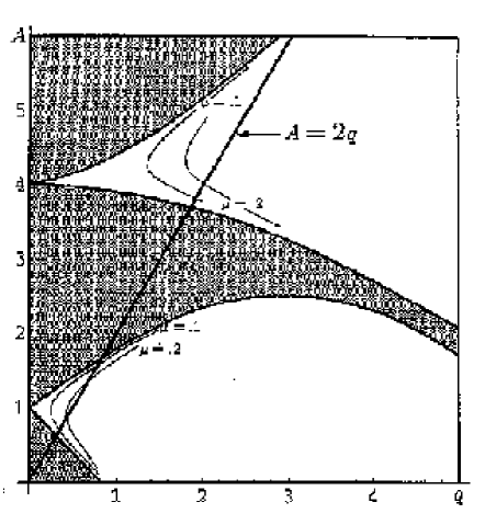
Before proceeding with this introduction to the theory of preheating we want to stress that we shall deal here only with bosonic reheating. Fermionic preheating is also conceivable although in this case the Pauli exclusion principle puts strong constraints on the production of particles from the quantum vacuum. Nevertheless it was soon realized that coherent oscillations of the inflaton can indeed lead to parametric production of fermions. We shall not treat this theory here but direct the reader to some seminal papers in the subject [281].

Parametric regimes

It should be stressed that very different regimes can be envisaged for the production of particles at different values of the relevant parameter $q$. For simplicity we shall describe them in a Minkowski spacetime ($a(t)=1$) discussing later the effects of expansion. We shall also consider a massless $\chi$ field.

Narrow resonance

A first possible regime corresponds to very small values of $q$ ($q\ll 1$ that is $g\Phi<m$) and takes the name of “narrow resonance”. In this case the particle production can be treated perturbatively and is concentrated in the first instability band for modes with $k^{2}\sim m^{2}_{\phi}(1-2q\pm q)$ [282]. Here the Floquet index takes the form [283]

$$\mu_{k}=\sqrt{\left(\frac{q}{2}\right)^{2}-\left(\frac{2k}{m_{\phi}}-1\right)^{2}}$$ (5.37)

The modes $\chi_{k}$ with $k\sim m$ grow as $\exp(qz/2)\sim\exp(g^{2}\Phi^{2}t/8m_{\phi})$ and the number of $\chi$ particles goes like $n_{k}(t)\sim\exp(2\mu^{(n)}_{k}z)\sim\exp(g^{2}\Phi^{2}t/4m_{\phi})$. This process can be interpreted as the conversion of two $\phi$ particles into a pair of $\chi$ particles with momenta $k\sim m$.

Figure 5.2: Mode and particle number amplification for the narrow resonance regime with $q\approx 1$. The time is in units of $m_{\phi}/2\pi$ and is hence equal to the number of oscillations of the inflaton field $\phi$. From [282].

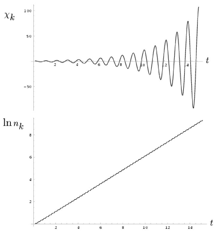
Broad resonance

A second important regime comes into action for wide oscillations of the inflaton, that is for $q\gg 1$ ($g\Phi\gg m)$. This is the so-called “broad resonance” regime. It is a typically non-perturbative process and leads rapidly to non-negligible backreaction by the created particles on the inflaton field. The resonance occurs not just in the first instability band but generically for modes above the $A=2q$ line in the Mathieu plot, Fig. 5.1, which have momenta $k^{2}/m^{2}=A-2q$. In the broad resonance regime the occupation numbers of the particles produced are extremely large, typically of order $n_{k}\sim 1/g^{2}$.

It is interesting to note that, due to the interaction term (5.29), the $\chi$ field acquires an effective mass $m_{\chi}(t)=g\phi(t)$ which, in this special regime, can be much larger that the inflaton mass. As a result, the typical frequency of oscillation of the $\chi$ field $\omega(t)=\sqrt{k^{2}+m_{\chi}^{2}(t)}$ becomes larger than that of the inflaton. This also implies that during most of the period of oscillation of $\phi$ the mass of the $\chi$ field changes adiabatically. Only for $\phi(t)\approx 0$, where the effective mass of the $\chi$ field is almost zero, is there violation of the adiabatic condition

$$\frac{{\mathrm{d}}\omega}{{\mathrm{d}}t}\leq\omega^{2}$$ (5.38)

and efficient production of particles as shown in Fig. 5.3.

Figure 5.3: Mode and particle number amplification for the broad resonance regime with $q\gg 1$. The time is in units of $m_{\phi}/2\pi$. Note the rapid oscillations in $\chi_{k}$ and the “stair-like” behaviour of the particle number. From [282].

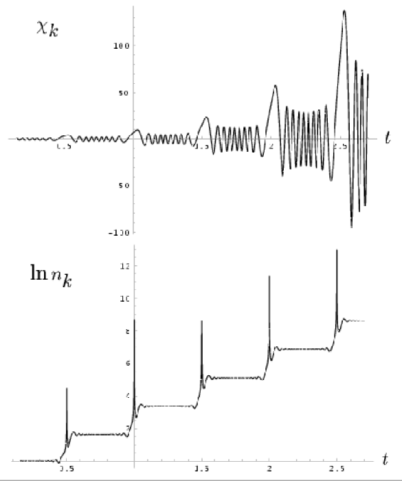
A final comment is in order. One should not think that arbitrarily high values for $q$ would lead to higher and higher bursts of particle creation. In fact, for $q\geq 10^{3}$, generally non-perturbative effects (like backreaction and rescattering) soon become crucial for determining the duration of the resonance regime and the final variance of both the $\chi$ and $\phi$ fields. We direct the reader to [282] for further insight into this subject.

Stochastic resonance

To conclude this short introduction to the post-inflationary preheating phase, we shall now briefly discuss the role of expansion which we have neglected so far. We can start by noticing that if expansion is included, then the modes suffer a redshift ${\mathbf{k}}\to{\mathbf{k}}/a(t)$ and the amplitude of the inflaton oscillations decreases in time as $t^{-1}$. This drives the parameters $A$ and $q$ towards zero and hence kills the parametric amplification.

Moreover it should be noted that Eq. (5.32) also tells us that the amplitude of the $\phi$ oscillations decreases very rapidly if their number is increased. Since $q\sim\Phi^{2}\sim 1/N^{2}$, only a few oscillations will be enough to greatly deplete $q$. This means that in the case of narrow resonance (when $q\ll 1$ from the beginning) the amplification is not able to start at all.

The former point is nevertheless an important one. In fact if we assume to start in a broad resonance regime then one can easily show that the field $\chi$ moves through several bands after a few oscillations. In fact in Mathieu theory the band number is given by $n=\sqrt{A}$ and so if the resonance happens mostly for $A\sim 2q$ one gets $n\sim\sqrt{2q}\sim g\Phi/(m_{\phi}\sqrt{2})$. If we take $m_{\phi}\approx 10^{-6}M_{\mathrm{Pl}}$, $g\approx 10^{-1}$ then, by using Eq. (5.32) and Eq. (5.34), one finds that after the first oscillation $n\approx 10^{4}$ but $n\approx 5\cdot 10^{3}$ after the second.

Therefore we see that even during a single oscillation the field does not remain in one instability band but moves through a thousand of them. The standard method for looking at particle production in a chosen instability band then fails completely here. It is nevertheless still possible to make a numerical analysis under suitable approximations. In [282] such an analysis is performed and shows a behaviour in which the particle number generally increases (discontinuously) but sometimes even decreases. The $X_{k}$ modes are defined via rescaling of the $\chi_{k}$ ones, $X_{k}=\chi_{k}(t/t_{0})$ where $t_{0}$ is the starting time. The occupation number of particles per mode can be constructed as

$$n_{k}=\frac{\omega_{k}}{2}\left(\frac{|\dot{X}_{k}|^{2}}{\omega_{k}^{2}}+|X_{k}|^{2}\right)-\frac{1}{2}$$ (5.39)

Figure 5.4: Mode and particle number amplification for the stochastic resonance regime with $q\sim 3\cdot 10^{3}$. Note the rapid oscillations in $\chi_{k}$ and the “stair-like” behaviour of the particle number but this time including several drops in the particle number. This is a purely quantum mechanical effect which would be impossible if these particles were in a classical state. From [282].

After this brief overview of the basic elements of the the theory of inflationary preheating we shall now discuss a different “channel” for parametric resonance to occur, the so-called “geometric preheating”. This original investigation has been made in collaboration with B.A. Bassett and most of the material presented here has been published in reference [20].

5.4 Geometric Reheating

The preheating theory which we have seen so far is based on the direct coupling between the inflaton and the quantum field to be produced. Although we have worked with the simple coupling term (5.29) other forms of coupling can be considered and other fields (such as fermions or vector bosons) can be coupled to the inflaton and eventually amplified by its oscillations. Obviously weak coupling will strongly depress any reheating mechanism (from (5.34) it is easy to see that small values of $g$ end up depressing the value of $q$).

One can nevertheless wonder whether there is the possibility, for some generic coupling, for this process to play an important role and whether gravity should not play a more active part in the process of preheating. In particular we have considered so far a minimally coupled scalar field $\chi(t,{\mathbf{x}})$ excluding any direct action of gravity.

Our starting point is that this last assumption is far from being generic. Renormalization group studies in curved spacetime [284, 285, 286] have shown that even if the bare coupling $\xi_{0}$ is minimal, after renormalization one should generically expect $\xi\not=0$. In particular, while in the infrared limit fixed points may correspond to a conformally invariant field ($m=0$, $\xi={1\over 6}$) , in different GUT models the coupling may also diverge, $|\xi|\rightarrow\infty$, in the UV limit [284, 288]. In both cases the nature of the preheating is very different from the standard models based on explicit self-interactions or particle-physics couplings between fields (see e.g. [282]).

Since we are particularly interested in the preheating regime which occurs when inflation ends, we are interested in the ultra-violet (UV) fixed points of the renormalization group equations. As a consequence of this we can assume a general non minimal coupling with possibly large values of the parameter $\xi$.

To be concrete, consider a generic FLRW universe described by the metric element (5.1) and a minimally coupled scalar field $\phi$ which is governed by the evolution equation (5.31).

Let us restrict ourselves to the quadratic potential (5.28) which we know to give, for $K=0$, an oscillatory behaviour of the field: $\phi=\Phi\sin(m_{\phi}t)$, with $\Phi\sim 1/m_{\phi}t$. In the following we shall try to preserve maximal generality but when results are derived specifically for the potential (5.28) we shall denote them with $\doteq$.

The energy density and pressure for a minimally coupled scalar field, treated as a perfect fluid, are

$$\mu=\kappa_{\mathrm{N}}\left({1\over 2}\dot{\phi}^{2}+V(\phi)\right),\qquad p=\kappa_{\mathrm{N}}\left({1\over 2}\dot{\phi}^{2}-V(\phi)\right),$$ (5.40)

where $\kappa_{\mathrm{N}}=8\pi G_{\mathrm{N}}$. This breaks down if the field is non-minimally coupled (an imperfect fluid treatment must be used), if the effective potential is not adequate [289], or if large density gradients exist. The FLRW Ricci tensor is [290]

$$R^{0}{}_{0} = 3\frac{\ddot{a}}{a}$$

$$R^{i}{}_{j} = \left[\frac{\ddot{a}}{a}+2\left(\frac{\dot{a}}{a}\right)^{2}+\frac{2K}{a^{2}}\right]\delta^{i}{}_{j}\,,$$ (5.41)

where as usual $i,j=1..3$. The Ricci scalar is :

$$R=6\left(\frac{\ddot{a}}{a}+\left(\frac{\dot{a}}{a}\right)^{2}+\frac{K}{a^{2}}\right)\,.$$ (5.42)

We now see that the curvature scalar can be expressed in terms of a combination of the derivatives of the FLRW scale factor. In order to express it directly as a function of the inflaton field and of its effective potential — we are assuming that at the onset of preheating the inflaton is still the dominant matter in the universe — we can look at the Raychaudhuri equation for the evolution of the expansion factor $\Theta=3\dot{a}/a$ 

$$\dot{\Theta}=-\frac{3\kappa_{\mathrm{N}}}{2}\dot{\phi}^{2}+\frac{3K}{a^{2}}\,,$$ (5.43)

We can also get information from the Friedmann equation (5.14) which takes the form

$$\Theta^{2}+{9K\over a^{2}}=3\kappa_{\mathrm{N}}\mu=3\kappa_{\mathrm{N}}\left({1\over 2}\dot{\phi}^{2}+V(\phi)\right)\,.$$ (5.44)

Using equations (5.43) and (5.44), one can systematically replace in (5.42) all factors of $\dot{a},\ddot{a}$ with factors of $\dot{\phi}$ and $V(\phi)$.

As an example, taking the usual quadratic potential, $K=0$ and $\dot{a}/(am_{\phi})\ll 1$, one may solve Eq. (5.44) perturbatively [292] obtaining

$$\Theta\doteq\frac{2}{t}\left[1-\frac{\sin 2m_{\phi}t}{2m_{\phi}t}\right]\,,$$ (5.45)

to first order in $\dot{a}/(am_{\phi})$. This is only valid after preheating when $\Phi\ll 1$ but shows that the expansion oscillates about the mean Einstein-de Sitter (eds) pressure-free solution. Eq. (5.45) can be integrated to give the scale factor:

$$a(t)\doteq\overline{a}\exp\left(\frac{\sin 2m_{\phi}t}{3m_{\phi}t}-\frac{2\mbox{ci}(2m_{\phi}t)}{3}\right)$$ (5.46)

where $\overline{a}=t^{2/3}$ is the background eds evolution, and $\mbox{ci}(m_{\phi}t)=-\int^{\infty}_{t}\cos(m_{\phi}z)/zdz$. This example explicitly demonstrates how by just temporal averaging (which yields $\overline{a}$) one would completely miss the oscillatory behaviour of the expansion factor. It is instead this feature that we shall use to get parametric resonance.

The basic idea which we shall follow is that the oscillations in the inflaton field induce an oscillatory behaviour in the expansion factor and hence in the Ricci scalar. It then follows that any field which is non-minimally coupled to gravity will be potentially subject to parametric amplification without the need for a direct coupling to the inflaton. In this sense this preheating channel, which can be called geometric reheating can be considered as a typical example of the dynamical Casimir effect in a periodic external field where the latter is the gravitational one.

In the following, we shall apply this simple idea to the case of scalar, vector and tensor fields.

5.4.1 Scalar fields

We start by considering the easiest case when $N$ massive scalar fields $\chi^{(\nu)}(t,{\mathbf{x}})$, $\nu=1\dots N$, are non-minimally coupled to gravity

$${\cal L}(x)=\frac{1}{2}\sum_{\nu}^{N}\left[g^{\alpha\beta}\nabla_{\alpha}\chi^{(\nu)}\nabla_{\beta}\chi^{(\nu)}+\left(m^{(\nu)}_{\chi}\chi^{(\nu)}\right)^{2}+\xi^{(\nu)}\left(\chi^{(\nu)}\right)^{2}R\right]$$ (5.47)

so we now have the inflaton, with potential $V(\phi)$, coupled only via gravity to the other scalar fields, which have no self-interactions, masses $m^{(\nu)}_{\chi}$ and non-minimal couplings $\xi^{(\nu)}$. The equation of motion for modes of the $\nu$-th field is:

$$\ddot{\chi}^{(\nu)}_{k}+\Theta\dot{\chi}^{(\nu)}_{k}+\left(\frac{k^{2}}{a^{2}}+\left(m^{(\nu)}_{\chi}\right)^{2}+\xi^{(\nu)}R\right)\chi^{(\nu)}_{k}=0\,,$$ (5.48)

From Eq (5.42,5.43,5.44) the Ricci scalar is given by

$$R=-\kappa_{\mathrm{N}}\dot{\phi}^{2}+4\kappa_{\mathrm{N}}V(\phi)~{}~{}~{}(K=0)\,.$$ (5.49)

We can now treat separately the cases of minimally and non-minimally coupled fields and investigate the different behaviour of the parametric amplification.

The minimally coupled case

Consider $\xi_{\nu}=0$. We can manipulate Eq. (5.48) by changing variables from $\chi^{(\nu)}_{k}$ to $\bar{\chi}^{(\nu)}_{k}=a^{3/2}\chi^{(\nu)}_{k}$ in order to remove the first derivative term. Then by making use of equations (5.43,5.44), we can reduce it to:

$$\frac{d^{2}\bar{\chi}^{(\nu)}_{k}}{dt^{2}}+\left[\frac{k^{2}}{a^{2}}+\left(m_{\chi}^{(\nu)}\right)^{2}+\kappa_{\mathrm{N}}{3\over 8}\dot{\phi}^{2}-\kappa_{\mathrm{N}}{3\over 4}V(\phi)+{3\over 4}{K\over{a^{2}}}\right]\bar{\chi}^{(\nu)}_{k}=0$$ (5.50)

where we have used the useful identity: $\Theta^{2}+\dot{\Theta}=3(\dot{a}^{2}/a^{2}+2\ddot{a}/a)$.

We can now see that there is parametric resonance just because the expansion $\Theta$ oscillates. In fact if we take the potential (5.28) then we can recover the Mathieu equation (5.35) by defining $z=m_{\phi}t+\pi/2$, and introducing the time-dependent parameters

$$A(k,t) \doteq {{4k^{2}+3K}\over{4a^{2}m^{2}_{\phi}}}+{\left(m^{(\nu)}_{\chi}\right)^{2}\over m^{2}_{\phi}}$$ (5.51)

$$q \doteq {3\over 16}\kappa_{\mathrm{N}}\Phi^{2}$$ (5.52)

From this we see that the production of particles is reduced as $m^{(\nu)}_{\chi}$ increases. Indeed, since $A\rightarrow m^{2}_{\chi}/m^{2}_{\phi}$, $q\rightarrow 0$ due to the expansion, production of minimally coupled bosons is rather weak and shuts off quickly due to horizontal motion on the stability chart. We stress that the production is, however, much stronger than that obtained in previous studies where the scale factor evolves monotonically [293]. This mild situation changes dramatically when a non-minimal coupling is introduced.

Non-minimal preheating

We now include the arbitrary non-minimal coupling $\xi_{\nu}$. Using Eq. (5.49) one can reduce Eq. (5.48) to:

$$\frac{d^{2}\bar{\chi}^{(\nu)}_{k}}{dt^{2}}+\left[\frac{4k^{2}+3K}{4a^{2}}+\left(m_{\chi}^{(\nu)}\right)^{2}+\kappa_{\mathrm{N}}\left(\frac{3}{8}-\xi_{\nu}\right)\dot{\phi}^{2}-\kappa_{\mathrm{N}}\left(\frac{3}{4}-4\xi_{\nu}\right)V(\phi)\right]\bar{\chi}^{(\nu)}_{k}=0$$ (5.53)

Adopting again the new variable $z=m_{\phi}t+\pi/2$, we can also express Eq. (5.53) in the Mathieu form (5.35). The time-dependent parameters are now

$$A(k,t) \doteq {{4k^{2}+3K}\over{4a^{2}m^{2}_{\phi}}}+{m^{2}_{\chi}\over m^{2}_{\phi}}+{{\kappa_{\mathrm{N}}\xi_{\nu}}\over 2}\Phi^{2}$$ (5.54)

$$q(t) \doteq {3\over 4}\kappa_{\mathrm{N}}\left({1\over 4}-\xi_{\nu}\right)\Phi^{2}$$ (5.55)

The crucial observation is that since $\xi_{\nu}$ is initially free to take on any value , $A(k)$ is not restricted to be either positive or small.  From Eq. (5.55) it is clear that $A(k)<0$ for sufficiently negative $\xi_{\nu}$. The possibility of a negative $A$ was the suggestion of the work by Greene et al [294]. However, in their model, this powerful negative coupling instability was only partially effective due to the non-zero vacuum expectation value acquired by the $\chi$ field due to its coupling, $g$, with the inflaton. Here we only have gravitational couplings and this constraint is removed.

Actually if we assume that $\xi_{\nu}<0$, then it is easy to see that for the $k=0$ mode and for $m_{\chi}/m_{\phi}\approx 0$ the relation between $A$ and $q$ is no longer, as in Eq. (5.34), $A\approx 2q$. Instead we now have that, in the same limits

$$A(k,t)\approx-\frac{2}{3}|q|+\frac{\kappa_{\mathrm{N}}}{8}\Phi^{2}$$ (5.56)

and so a negative $A$ (induced when $\xi_{\nu}<0$) implies that the properties of resonance are quite different in the $\xi_{\nu}>0$ case.

Figure 5.5: Band structure for $\xi_{\nu}<0$, from [295].

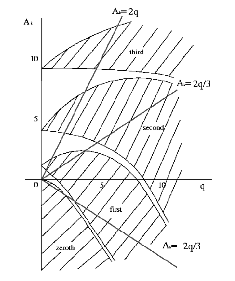
As shown in Fig. 5.5, the regions with $A<0$ of the $(A,q)$ plane possess a new instability band (sometimes called the zeroth instability band) which extends below some critical curve located approximately at $A\approx-q^{2}/2$ for small $|q|$. The line $A=-2q/3$ crosses this curve for $q\approx 1.4$ and so since $q$ drops below unity because of the cosmological expansion, there are still some modes in the zeroth band [295].

When $2|q|/3>|A|\gg 1$ we have $\mu_{k}\sim|q|^{1/2}\simeq(6\pi G_{\mathrm{N}}|\xi_{\nu}|)^{1/2}\Phi$ along the physical separatrix $A=\kappa_{\mathrm{N}}\Phi^{2}/8-2|q|/3$. Since the renormalized $|\xi_{\nu}|$ may have very large values, this opens the way to exceptionally efficient reheating - see Figs. (5.6,5.7) - via resonant production of highly non-minimally coupled fields with important consequences for GUT baryogenesis [294] and non-thermal symmetry restoration.

For example, let us consider $m_{\phi}\simeq 2\times 10^{13}GeV$ as required to match CMB anisotropies $\Delta T/T\sim 10^{-5}$. Then GUT baryogenesis with massive bosons $\chi$ with $m_{\chi}>10^{14}GeV$ simply requires that geometric preheating with $A<0$ happens with $\xi_{\nu}<-(\kappa_{\mathrm{N}}\Phi^{2})^{-1}10^{2}$. Instead if one requires the production of GUT-scale gauge bosons with masses $m_{\mathrm{gb}}\sim 10^{16}GeV$ this is still possible if the associated non-minimal coupling is of order $\xi_{\nu}\sim-(\kappa_{\mathrm{N}}\Phi^{2})^{-1}10^{6}$. Such coupling values have been considered in, for example [296]. The massive bosons with $m_{\chi}\sim 10^{14}GeV$ can be produced in the usual manner via parametric resonance if $\xi_{\nu}>0$, but this process is weaker (c.f. [297, 295]).

Figure 5.6: The evolution of the $k=0$ mode (with $m_{\nu}^{2}/m_{\phi}^{2}\simeq 1$), as a function of time and of the non-minimal coupling parameter $\xi_{\nu}$. For positive $\xi_{\nu}$ the evolution is qualitatively that of the standard preheating with resonance bands. However, for negative $A$ (negative $\xi_{\nu}$) the solution changes qualitatively and there is a negative coupling instability. There are generically no stable bands and the Floquet index corresponding to $-|\xi_{\nu}|$ is much larger, scaling as $\mu_{k}\sim|\xi_{\nu}|^{1/2}$.

Figure 5.7: A slice of the spectrum in fig. 5.6 at $t=5$ as a function of the non-minimal coupling $\xi_{\nu}$. The qualitative differences between $\xi_{\nu}<0$ and $\xi_{\nu}>0$ are clear.

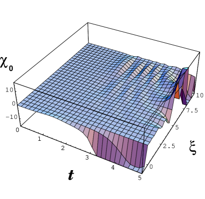
Since the coupling between $\phi$ and $\chi$ is purely gravitational, backreaction effects in the standard sense (see [282, 289]) cannot shut off the resonance (they are generally based on direct coupling terms like (5.29)). The inflaton continues to oscillate and produce non-minimally coupled particles, receiving no corrections to $m_{\phi,\mathrm{eff}}^{2}$ from $\langle\chi^{2}\rangle$ (as is instead the case if one has, for example, a coupling term of the form $g\chi^{2}\phi^{2}/2$). Understanding when the parametric resonance is shut down in geometric preheating is therefore rather difficult.

The standard method is to establish the time when the resonance is stopped by the growth of $A(k)$ which pushes the $k=0$ mode out of the dominant first resonance band. In our case we must understand how $A(k)$ changes as the $\chi$-field gains energy and alters the Ricci curvature. In fact the basic mechanism which one can expect is that at some time the energy transferred into the $\chi$ field will be enough so that it is no longer possible to neglect its backreaction on the Ricci scalar.

If one assumes that most of the energy goes into the $\chi_{0}$ mode, then the change to the Ricci curvature can be expressed as $\delta R_{\chi}=8\pi(E-S)$, where [298]:

$$E=\frac{G_{\mathrm{eff}}}{G_{\mathrm{N}}}\left[\frac{\dot{\chi}_{0}^{2}}{2}+\frac{m_{\chi}^{2}\chi_{0}^{2}}{2}-12\xi_{\nu}\chi_{0}\dot{\chi}_{0}\frac{\dot{a}}{a}\right]$$ (5.57)

is the $T^{00}$ component of the $\chi$ stress tensor, and

$$S=\frac{3G_{\mathrm{eff}}}{1+192\pi G_{\mathrm{eff}}G_{\mathrm{N}}\xi_{\nu}^{2}\chi_{0}^{2}}\left[\frac{\dot{\chi}_{0}^{2}}{2}-\frac{m_{\chi}^{2}\chi^{2}_{0}}{2}+4\xi_{\nu}\left(\frac{\dot{a}^{2}}{a^{2}}-\chi_{0}\dot{\chi}_{0}\frac{\dot{a}}{a}-m_{\chi}^{2}\chi_{0}^{2}\right)+64\pi G_{\mathrm{N}}\xi_{\nu}^{2}\chi_{0}^{2}E\right]$$ (5.58)

is the spatial trace of the stress tensor $T^{i}{}_{i}$ corresponding to $3p$ in the perfect fluid case. (In the above formulae $G_{\mathrm{eff}}=G_{\mathrm{N}}/(1+16\pi G_{\mathrm{N}}\xi_{\nu}\chi^{2})$ is the effective gravitational constant.)

Since $\chi_{0}$ is rapidly growing, the major contribution of $\delta R_{\chi}$ will be to $A(k)$, causing a rapid vertical movement on the instability chart. Once $\delta A+A>2|q|+|q|^{1/2}$, the resonance is shut off. If $\xi_{\nu}<0$, most of the decaying $\phi$ energy is pumped into the small $k$ modes (see Fig. 5.7). Subsequently we expect the oscillations in $\chi_{0}$ to produce a secondary resonance due to the self-interaction and non-linearity of Eqs (5.57,5.58).

5.4.2 Vector fields

Until now, reheating studies have been limited to minimally-coupled scalar fields, fermions and gauge bosons [299]. In the case of vector fields the minimum one can do to preserve gauge-invariance is to couple to a complex scalar field via the current since real scalar fields carry no quantum numbers. We consider here only vacuum vector resonances, however.

A massive spin–1 vector field in curved spacetime satisfies the equations:

$$(-\nabla_{a}\nabla^{a}+m_{{\cal A}}^{2}){\cal A}^{b}+R^{b}{}_{a}{\cal A}^{a}=0$$ (5.59)

These equations are equivalent to the Maxwell–Proca equations for the vector potential ${\cal A}_{a}$ only after an appropriate gauge choice which removes one unphysical polarization. In our case we shall use the so-called tridimensional transversal constraint:

$${\cal A}_{0}=0,~{}~{}~{}\nabla^{i}{\cal A}_{i}=0$$ (5.60)

This set is equivalent to the Lorentz gauge, although it does not conserve the covariant form of the latter. Nonetheless, in either case, gauge-invariant quantities such as the radiation energy density, are unaffected.

In a FLRW background, the Ricci tensor is diagonal, which together with the gauge choice (5.60) and expansion over eigenfunctions, ensures the decoupling of the set of equations (5.59). We can reduce the system to a set of decoupled Mathieu equations. For $K=0$ the Ricci tensor is (see Eq. 5.41)

$$R^{a}{}_{b}=\kappa_{\mathrm{N}}V(\phi)\delta^{a}{}_{b}-\kappa_{\mathrm{N}}\dot{\phi}^{2}\delta^{a}{}_{0}\delta^{0}{}_{b}\,,$$ (5.61)

which leads to the Mathieu parameters for the spatial components $(a^{3/2}{\cal A}^{i})$

$$A(k)\doteq\frac{k^{2}}{a^{2}m_{\phi}^{2}}+\frac{m_{{\cal A}}^{2}}{m_{\phi}^{2}}+2q~{}~{}~{},~{}~{}q\doteq\frac{\kappa_{\mathrm{N}}\Phi^{2}}{8}$$ (5.62)

showing that vector fields are also parametrically amplified (albeit weakly) during reheating as in the scalar case.

5.4.3 The graviton case

It has been shown using the electric and magnetic parts of the Weyl tensor [300] that there exists a formal analogy between the scalar field and graviton cases during resonant reheating. Here we will show that the correspondence also holds in the Bardeen formalism. The gauge-invariant (at first order) transverse-traceless (TT) metric perturbations $h_{ij}$ describe gravitational waves in the classical limit. In the Heisenberg picture one expands over eigenfunctions, $Y_{ab}$ of the tensor Laplace–Beltrami operator with scalar mode functions $h_{k}$, which satisfy the equation of motion:

$$\ddot{h}_{k}+\Theta\dot{h}_{k}+\left(\frac{k^{2}+2K}{a^{2}}\right)h_{k}=0\,,$$ (5.63)

or equivalently

$$(a^{3/2}h_{k})\ddot{}+\left(\frac{k^{2}+2K}{a^{2}}+\frac{\textstyle 3}{4}p\right)(a^{3/2}h_{k})=0\,,$$ (5.64)

where $p=\kappa_{\mathrm{N}}(\dot{\phi}^{2}/2-V)$ is the pressure. This gives a time-dependent Mathieu equation (c.f. Eq. 5.52) with parameters:

$$A(k)\doteq\frac{k^{2}+2K}{a^{2}m_{\phi}^{2}}~{}~{},~{}~{}q\doteq-\frac{3\kappa_{\mathrm{N}}\Phi^{2}}{16}\,.$$ (5.65)

In this case, a negative coupling instability is impossible and only for $\Phi\sim M_{\mathrm{Pl}}$ is there significant graviton production. Note, however, that if temporal averaging is used, the average equation of state is that of dust, $\overline{p}=0$. Eq. (5.64) then predicts (falsely) that there is no resonant amplification of gravitational waves since the value of $q$ corresponding to the temporarily averaged evolution vanishes.

5.4.4 Discussion

We have described a new — geometric — reheating channel after inflation, one which occurs solely due to gravitational couplings. While this is not very strong in the gravitational wave and minimally coupled scalar field cases, it can be very powerful in the non-minimally coupled case, either due to broad-resonance ($\xi\gg 1$) or negative coupling ($\xi<0$) instabilities. Particularly in the latter case, it is possible to produce large numbers of bosons which are significantly more massive than the inflaton, as required for GUT baryogenesis. It further gives rise to the possibility that the post-inflationary universe may be dominated by non-minimally coupled fields. These must be treated as imperfect fluids which would thus alter both density perturbation and background spacetime evolution, which are known to be significantly different [301] than in the simple perfect fluid case. We have further seen a unified approach to resonant production of vector and tensor fields during reheating in analogy to the scalar case.

With the study of this nice example of parametric resonance due to a non-stationary gravitational field, we close our discussion about inflation. In what follows we shall move our attention to a class of models that try to present an alternative to this paradigm. In particular we shall propose a particular implementation of the varying speed of light cosmologies. This investigation is mainly included in [21] and was done in collaboration with Bruce A. Bassett, Carmen Molina–París and Matt Visser.

5.5 Alternatives to inflation?

High-energy cosmology is flourishing into a subject of observational riches but theoretical poverty. Inflation stands as the only well-explored paradigm for solving the puzzles of the early universe. This monopoly is reason enough to explore alternative scenarios and new angles of attack. Variable–Speed–of–Light (VSL) cosmologies have recently generated considerable interest as alternatives to cosmological inflation which serve both to sharpen our ideas regarding falsifiability of the standard inflationary paradigm, and also to provide a contrasting scenario that is hopefully amenable to observational test. The major variants of VSL cosmology under consideration are those of Clayton–Moffat [302, 303, 304, 305, 306] and Albrecht–Barrow–Magueijo [307, 308, 309, 310, 311], plus recent contributions by Avelino–Martins [312], Drummond [313], Kiritsis [314], and Alexander [315]. The last two are higher-dimensional, brane-inspired implementations.

Given this wide variety of implementations of the VSL idea it is difficult to present it as a paradigm. Roughly speaking one can cast the basic ideas behind these models in the following way. The covariance of General Relativity means that the set of cosmological models consistent with the existence of the apparently universal class of preferred rest frames defined by the CMBR, is very small and non-generic. Inflation alleviates this problem by making the flat FLRW model an attractor within the set of almost–FLRW models, at the cost of violating the strong energy condition. Most of the above quoted VSL cosmologies, by contrast, sacrifice (or at the very least, grossly modify) Lorentz invariance at high energies, by allowing the speed of light to vary in time (and hence setting up a preferred reference system) in order to mitigate the cosmological puzzles discussed above. This is not strictly true for all of the conceivable VSL models. We shall see how it is possible to build up VSL frameworks where Lorentz invariance is not explicitly violated.

In the following we shall discuss how a general VSL model can be built up and justified and consider the internal consistency of cosmological models characterized by a variable speed of light.

5.5.1 Varying–Speed–of–Light Cosmologies

As a starting point for our investigation we want to assess the internal consistency of the VSL idea and ask to what extent it is compatible with Einstein gravity. This is not a trivial issue: Ordinary Einstein gravity has the constancy of the speed of light built into it at a fundamental level; $c$ is the “conversion constant” that relates time to space. We need to use $c$ to relate the zeroth coordinate to time: ${\mathrm{d}}x^{0}=c\;{\mathrm{d}}t$. Thus, simply replacing the constant $c$ by a position-dependent variable $c(t,{\mathbf{x}})$, and writing ${\mathrm{d}}x^{0}=c(t,{\mathbf{x}})\;{\mathrm{d}}t$ is a suspect proposition.

Indeed, the choice ${\mathrm{d}}x^{0}=c(t,{\mathbf{x}})\;{\mathrm{d}}t$ is a coordinate dependent statement. It depends on how one slices up the spacetime with spacelike hypersurfaces. Different slicings would lead to different metrics, and so one has destroyed the coordinate invariance of the theory right at step one. This is not a good start for the VSL programme, as one has performed an act of extreme violence to the mathematical and logical structure of General Relativistic cosmology.

Another way of viewing the same problem is this. Start with the ordinary FLRW metric

$${\mathrm{d}}s^{2}=-c^{2}\;{\mathrm{d}}t^{2}+a(t)^{2}\;h_{ij}\;{\mathrm{d}}x^{i}\;{\mathrm{d}}x^{j},$$ (5.66)

and compute the Einstein tensor. In the natural orthonormal basis one can write

$$G_{\hat{t}\hat{t}} = {3\over a(t)^{2}}\;\left[{\dot{a}(t)^{2}\over c^{2}}+K\right],$$ (5.67)

$$G_{\hat{\imath}\hat{\jmath}} = -\frac{\delta_{\hat{\imath}\hat{\jmath}}}{a(t)^{2}}\;\left[2{a(t)\;\ddot{a}(t)\over c^{2}}+{\dot{a}(t)^{2}\over c^{2}}+K\right],$$ (5.68)

with the spatial curvature $K=0,\pm 1$. If one replaces $c\to c(t)$ in the metric, then the physics does not change since this particular “variable speed of light” can be undone by a coordinate transformation: $c\;{\mathrm{d}}t_{\mathrm{n}ew}=c(t)\;{\mathrm{d}}t$. While a coordinate change of this type will affect the (coordinate) components of the metric and the (coordinate) components of the Einstein tensor, the orthonormal components and (by extension) all physical observables (which are coordinate invariants) will be unaffected. Superficially more attractive, (because it has observable consequences), is the possibility of replacing $c\to c(t)$ directly in the Einstein tensor. (This is the route chosen by Barrow et al.[308, 309, 310], by Albrecht et al. [307, 311], and by Avelino and Martins [312].) Then

$$G_{\hat{t}\hat{t}}^{\mathrm{modified}} = {3\over a(t)^{2}}\;\left[{\dot{a}(t)^{2}\over c(t)^{2}}+K\right],$$ (5.69)

$$G_{\hat{\imath}\hat{\jmath}}^{\mathrm{modified}} = -{\delta_{\hat{\imath}\hat{\jmath}}\over a(t)^{2}}\;\left[2{a(t)\;\ddot{a}(t)\over c(t)^{2}}+{\dot{a}(t)^{2}\over c(t)^{2}}+K\right].$$ (5.70)

Unfortunately, if one does so, the modified “Einstein tensor” is not covariantly conserved (it does not satisfy the contracted Bianchi identities), and this modified “Einstein tensor” is not obtainable from the curvature tensor of any spacetime metric. Indeed, if we define a timelike vector $V^{\mu}=(\partial/\partial t)^{\mu}=(1,0,0,0)$ a brief computation yields

$$\nabla_{\mu}G_{\mathrm{modified}}^{\mu\nu}\propto\dot{c}(t)\;V^{\nu}.$$ (5.71)

Thus, violations of the Bianchi identities for this modified “Einstein tensor” are an integral part of this particular way of trying to make the speed of light variable. (In the Barrow et al. approach they prefer to define modified Bianchi identities by moving the RHS above over to the LHS. They then speak of these modified Bianchi identities as being satisfied. Nevertheless the usual Bianchi identities are violated in their formalism.)

If one couples this modified “Einstein tensor” to the stress-energy via the Einstein equation

$$G_{\mu\nu}={8\pi\;G_{\mathrm{N}}\over c^{4}}\;T_{\mu\nu},$$ (5.72)

then the stress-energy tensor divided by $c^{4}$ cannot be covariantly conserved either (here we do not need to specify just yet if we are talking about a variable $c$ or a fixed $c$), and so $T^{\mu\nu}/c^{4}$ cannot be variationally obtained from any action. [The factor of $c^{4}$ is introduced to make sure that all components of the stress-energy tensor have the dimensions of energy density, $\varepsilon$ (the same dimensions as pressure, $p$.) When needed, mass density will be represented by $\rho$.] This is an enormous amount of physics to sacrifice before even properly getting started, and we do not wish to pursue this particular avenue any further — it is offered as an example of the sort of fundamental things that can go wrong if one is not careful when setting up a VSL cosmology.

Apart from the mathematical consistency of the VSL approach, there is another fundamental issue to be addressed. If $c\to c(t)$ everywhere in the theory, how could we tell? Since our rulers and clocks are all affected by the change, why does not everything cancel out, relegating VSL-type approaches to being physically meaningless changes in the system of units? In [307] it is properly pointed out that it is only through changes in dimensionless numbers that any physical effect could be detected. It is common to phrase the discussion in terms of the fine structure constant $\alpha$

$$\alpha={e^{2}\over 4\pi\;\epsilon_{0}\;\hbar\;c}\approx{1\over 137}.$$ (5.73)

Unfortunately, if one chooses $\alpha$ as the relevant probe, it is difficult, if not impossible, to distinguish a variable speed of light from a variable Planck constant, a variable electric charge, or a variation in the permeability of the vacuum.

Proposal

From the former discussion it should now be clear that if one wants to uniquely specify that it is the speed of light that is varying, then one should seek a theory that contains two natural speed parameters, call them $c_{\mathrm{photon}}$ and $c_{\mathrm{gravity}}$ ( $c_{\mathrm{gravity}}$ is the speed at which small gravitational disturbances propagate), and then ask that the ratio of these two speeds is a time dependent quantity. Naturally, once we go beyond idealized FLRW cosmologies, to include perturbations, we will let this ratio depend on space as well as time. Thus we would focus attention on the dimensionless ratio

$$\zeta\equiv{c_{\mathrm{photon}}\over c_{\mathrm{gravity}}}.$$ (5.74)

With this idea in mind, it is simplest to take $c_{\mathrm{gravity}}$ to be fixed and position-independent and to set up the mathematical structure of differential geometry needed in implementing Einstein gravity: ${\mathrm{d}}x^{0}=c_{\mathrm{gravity}}\;{\mathrm{d}}t$, the Einstein–Hilbert action, the Einstein tensor, etc.. One can reserve $c_{\mathrm{photon}}$ for photons, and give an objective meaning to the VSL concept. (Observationally, as recently emphasized by Carlip [316], direct experimental evidence tells us that in the current epoch $c_{\mathrm{gravity}}\approx c_{\mathrm{photon}}$ to within about one percent tolerance. This limit is perhaps a little more relaxed than one would have naively expected, but the looseness of this limit is a reflection of the fact that direct tests of General Relativity are difficult due to the weakness of the gravitational coupling $G_{\mathrm{N}}$.) This approach naturally leads us into the realm of two-metric theories, and the next section will be devoted to discussing the origin of our proposal. In brief, we will advocate using at least two metrics: a spacetime metric $g_{\alpha\beta}$ describing gravity, and a second “effective metric” $[g^{\mathrm{e}m}]_{\alpha\beta}$ describing the propagation of photons. Other particle species could, depending on the specific details of the model we envisage, couple either to their own “effective metric”, to $g$, or to $g^{\mathrm{e}m}$.

Precursors

We have seen in chapter 1 (in section 1.2) that the basic idea of a quantum-induced effective metric, which affects only photons and differs from the gravitational metric, is actually far from radical. As we said, “anomalous” (larger than $c_{\mathrm{gravity}}$) photon speeds have been calculated in relation to the propagation of light in the Casimir vacuum [34, 35, 36], as well as in gravitational fields [37, 38, 39, 40]. Moreover we also noted that in recent papers [42, 43] it has been stressed that such behaviour can be described in a geometrical way by the introduction of an effective metric which is related to the spacetime metric and the renormalized stress-energy tensor. In curved spaces the natural generalization of Eq. (1.47) takes the form

$$[g_{\mathrm{em}}^{-1}]^{\mu\nu}=A\;g^{\mu\nu}+B\;\langle\psi|T^{\mu\nu}|\psi\rangle,$$ (5.75)

where $A$ and $B$ depend on the detailed form of the effective (one-loop) Lagrangian for the electromagnetic field.

Warning: We will always raise and lower indices using the spacetime metric $g$. This has the side-effect that one can no longer use index placement to distinguish the matrix $[g_{\mathrm{em}}]$ from its matrix inverse $[g_{\mathrm{em}}^{-1}]$. (Since $[g_{\mathrm{em}}]^{\mu\nu}\equiv g^{\mu\sigma}\;g^{\nu\rho}\;[g_{\mathrm{em}}]_{\sigma\rho}\neq[g_{\mathrm{em}}^{-1}]^{\mu\nu}.$) Accordingly, whenever we deal with the EM metric, we will always explicitly distinguish $[g_{\mathrm{em}}]$ from its matrix inverse $[g_{\mathrm{em}}^{-1}]$.

It is important to note that such effects can safely be described without needing to take the gravitational back reaction into account. The spacetime metric $g$ is only minimally affected by the vacuum polarization, because the formula determining $[g^{\mathrm{em}}]$ is governed by the fine structure constant, while backreaction on the geometry is regulated by Newton’s constant.

Although these deviations from standard propagation are extremely small for the cases quoted above (black holes and the Casimir vacuum) we can ask ourselves if a similar sort of physics could have been important in the early evolution of our universe. Drummond and Hathrell [37] have, for example, computed one-loop vacuum polarization corrections to QED in the presence of a gravitational field. They show that at low momenta the effective Lagrangian is

$${\cal L}=-\frac{1}{4}\;F_{\mu\nu}\;F^{\mu\nu}-\frac{1}{4m_{e}^{2}}(\beta_{1}\;R\;F_{\mu\nu}\;F^{\mu\nu}+\beta_{2}\;R_{\mu\nu}\;F^{\mu\alpha}\;F^{\nu}{}_{\alpha})-\frac{\beta_{3}}{4m_{e}^{2}}\;R_{\mu\nu\alpha\beta}\;F^{\mu\alpha}\;F^{\nu\beta}\,.$$ (5.76)

They were able to compute the low momentum coefficients $\beta_{i},i=1\dots 3$, but their results are probably not applicable to the case $R/m_{e}\gg 1$ of primary interest here. It is the qualitative structure of their results that should be compared with our prescriptions as developed in the next section.

Lorentz invariance

Actually our approach can be seen as a development of the above results. We shall use some classical (external) field to polarize the vacuum of some quantum fields and hence split the degeneracy (in the sense described above) between the (effective) null cones of various species of particles.

It is important to understand that in these two-metric models the Lorentz symmetry is broken in a “soft” manner, rather than in a “hard” manner. This “soft” breaking of Lorentz invariance, due to the nature of the ground state or initial conditions, is qualitatively similar to the notion of spontaneous symmetry breaking in particle physics, whereas “hard” breaking, implemented by explicitly non-invariant terms in the Lagrangian, is qualitatively similar to the notion of explicit symmetry breaking in particle physics.

In particular it can be illuminating to consider the Euler–Heisenber Lagrangian (1.44) that induces the Scharnhorst effect (we write it again here for the convenience of the reader)

$${\cal L}=\frac{{\mathbf{E}}^{2}-{\mathbf{B}}^{2}}{8\pi}+\frac{\alpha^{2}}{2^{3}\cdot 3^{2}\cdot 5\pi^{2}m_{e}^{4}}\left[\left({\mathbf{E}}^{2}-{\mathbf{B}}^{2}\right)^{2}+7\left({\mathbf{E}}\cdot{\mathbf{B}}\right)\right]$$ (5.77)

It is easy to see that the second term on the right hand side (the one that induces the non-linearity and the anomalous propagation of the photons) is, by itself, Lorentz invariant. The anisotropic speed of propagation of light is due to the fact that the Lorentz symmetry breaking is induced by the external conditions (the parallel plates) which reflects in a non-Lorentz invariant (Casimir) ground state.

As a final remark it has to be pointed out that the VSL implementations based on two-metric theories, which we shall pursue in the next section, are certainly closer in spirit to the approaches of Moffat et al. [302, 303, 304, 305, 306] and Drummond [313], than to the Barrow et al. [308, 309, 310, 307, 311] and Avelino–Martins [312] prescriptions. In this sense parts of this investigation can be viewed as an extension (and criticism) of those models.

5.6 The $\chi$VSL framework

Based on the preceding discussion, we shall write, as the first step towards making a VSL cosmology “geometrically sensible”, a two-metric theory in the form

$$S_{I}=\int{\mathrm{d}}^{4}x\sqrt{-g}\;\left\{R(g)+{\cal L}_{\mathrm{matter}}(g)\right\}+\int{\mathrm{d}}^{4}x\sqrt{-g_{\mathrm{em}}}\;\left\{[g_{\mathrm{em}}^{-1}]^{\alpha\beta}\;F_{\beta\gamma}\;[g_{\mathrm{em}}^{-1}]^{\gamma\delta}\;F_{\delta\alpha}\right\}$$ (5.78)

Note that here we have just made the first of many choices. In fact we chose the volume element for the electromagnetic Lagrangian to be $\sqrt{-g_{\mathrm{em}}}$ rather than, say $\sqrt{-g}$. This has been done to do minimal damage to the electromagnetic sector of the theory. As long as we confine ourselves to making only electromagnetic measurements this theory is completely equivalent to ordinary curved space electromagnetism in the spacetime described by the metric $g_{\mathrm{em}}$. As long as we only look at the “matter” fields it is only the “gravity metric” $g$ that is relevant.

Since the photons couple to a second, separate metric, distinct from the spacetime metric that describes the gravitational field, we can now give a precise physical meaning to VSL. If the two null-cones (defined by $g$ and $g_{\mathrm{em}}$, respectively) do not coincide one has a VSL cosmology. Gravitons and all matter except for photons, couple to $g$. Photons couple to the electromagnetic metric $g_{\mathrm{em}}$. A more subtle model is provided by coupling all of the gauge bosons to $g_{\mathrm{em}}$, but everything else to $g$.

$$S_{II}=\int{\mathrm{d}}^{4}x\sqrt{-g}\;\left\{R(g)+{\cal L}_{\mathrm{ferm}}(g,\psi)\right\}+\int{\mathrm{d}}^{4}x\sqrt{-g_{\mathrm{em}}}\;\mathrm{Tr}\left\{[g_{\mathrm{em}}^{-1}]^{\alpha\beta}\;F_{\beta\gamma}^{\mathrm{gauge}}\;[g_{\mathrm{em}}^{-1}]^{\gamma\delta}\;F_{\delta\alpha}^{\mathrm{gauge}}\right\}$$ (5.79)

For yet a third possibility: couple all the matter fields to $g_{\mathrm{em}}$, keeping gravity as the only field coupled to $g$. That is

$$S_{III}=\int{\mathrm{d}}^{4}x\sqrt{-g}\;R(g) + \int{\mathrm{d}}^{4}x\sqrt{-g_{\mathrm{em}}}\;\left\{{\cal L}_{\mathrm{ferm}}(g_{\mathrm{em}},\psi)\right\}$$ (5.80)

$$+ \int{\mathrm{d}}^{4}x\sqrt{-g_{\mathrm{em}}}\;\mathrm{Tr}\left\{[g_{\mathrm{em}}^{-1}]^{\alpha\beta}\;F_{\beta\gamma}^{\mathrm{gauge}}\;[g_{\mathrm{em}}^{-1}]^{\gamma\delta}\;F_{\delta\alpha}^{\mathrm{gauge}}\right\}$$

Note that we have used ${\mathrm{d}}x^{0}=c\;{\mathrm{d}}t$, with the $c$ in question being $c_{\mathrm{gravity}}$. It is this $c_{\mathrm{gravity}}$ that should be considered fundamental, as it appears in the local Lorentz transformations that are the symmetry group of all the non-electromagnetic interactions. It is just that $c_{\mathrm{gravity}}$ is no longer the speed of “light”.

Most of the following discussion will focus on the first model $S_{I}$, but it is important to realize that VSL cosmologies can be implemented in many different ways, of which the models I, II, and III are the cleanest exemplars. We will see later that there are good reasons to suspect that model III is more plausible than models I or II, but we concentrate on model I for its pedagogical clarity. If one wants a model with even more complexity, one could give a different effective metric to each particle species. A model of this type would be so unwieldy as to be almost useless.

If there is no relationship connecting the EM metric to the gravity metric, then the theory has too much freedom to be useful, and the equations of motion are under-determined. To have a useful theory we need to postulate some relationship between $g$ and $g_{\mathrm{em}}$, which in the interest of simplicity we take to be algebraic. A particularly simple electromagnetic (EM) metric which one can consider is

$$[g_{\mathrm{em}}]_{\alpha\beta}=g_{\alpha\beta}-(A\;M^{-4})\;\nabla_{\alpha}\chi\;\nabla_{\beta}\chi,$$ (5.81)

with the inverse metric

$$[g_{\mathrm{em}}^{-1}]^{\alpha\beta}=g^{\alpha\beta}+(A\;M^{-4})\;{\nabla^{\alpha}\chi\;\nabla^{\beta}\chi\over 1-(A\;M^{-4})\;(\nabla^{\alpha}\chi)^{2}}.$$ (5.82)

Here we have introduced a dimensionless coupling $A$ and taken $\hbar=c_{\mathrm{gravity}}=1$, in order to give the scalar field $\chi$ its canonical dimensions of mass-energy. The normalization energy scale, $M$, is defined in terms of $\hbar$, $G_{\mathrm{N}}$, and $c_{\mathrm{gravity}}$. The EM lightcones can be much wider than the standard (gravity) ones without inducing a large backreaction on the spacetime geometry from the scalar field $\chi$, provided $M$ satisfies $M_{\mathrm{Electroweak}}<M<M_{\mathrm{Pl}}$. The presence of this dimensional coupling constant implies that when viewed as a quantum field theory, $\chi$VSL cosmologies will be non-renormalizable. In this sense the energy scale $M$ is the energy at which the non-renormalizability of the $\chi$ field becomes important. (This is analogous to the Fermi scale in the Fermi model for weak interactions, although in our case $M$ could be as high as the GUT scale). Thus, $\chi$VSL models should be viewed as “effective field theories” valid for sub-$M$ energies. In this regard $\chi$VSL models are certainly no worse behaved than many of the current models of cosmological inflation and/or particle physics.

The evolution of the scalar field $\chi$ will be assumed to be governed by some VSL action

$$S_{\mathrm{VSL}}=\int{\mathrm{d}}^{4}x\sqrt{-g}\;{\cal L}_{\mathrm{VSL}}(\chi).$$ (5.83)

We can then write the complete action for model I as

$$S_{I} = \int{\mathrm{d}}^{4}x\sqrt{-g}\;\left\{R(g)+{\cal L}_{\mathrm{matter}}\right\}+\int{\mathrm{d}}^{4}x\sqrt{-g_{\mathrm{em}}(\chi)}\;\left\{[g_{\mathrm{em}}^{-1}]^{\alpha\beta}(\chi)\;F_{\beta\gamma}\;[g_{\mathrm{em}}^{-1}]^{\gamma\delta}(\chi)\;F_{\delta\alpha}\right\}$$ (5.84)

$$+ \int{\mathrm{d}}^{4}x\sqrt{-g}\;{\cal L}_{\mathrm{VSL}}(\chi)+\int{\mathrm{d}}^{4}x\sqrt{-g}\;{\cal L}_{\mathrm{NR}}(\chi,\psi),$$

where ${\cal L}_{\mathrm{N}R}(\chi,\psi)$ denotes the non-renormalizable interactions of $\chi$ with the standard model.

Let us suppose the potential in this VSL action has a global minimum, but the $\chi$ field is displaced from this minimum in the early universe: either trapped in a metastable state by high-temperature effects or displaced due to chaotic initial conditions. The transition to the global minimum may be either of first or second order and during it $\nabla_{\alpha}\chi\neq 0$, so that $g_{\mathrm{em}}\neq g$. Once the true global minimum is achieved, $g_{\mathrm{em}}=g$ again. Since one can arrange $\chi$ today to have settled to the true global minimum, current laboratory experiments would automatically give $g_{\mathrm{em}}=g$.

It is only via observational cosmology, with the possibility of observing the region where $g_{\mathrm{em}}\neq g$ that we would expect VSL effects to manifest themselves. We will assume the variation of the speed of light to be confined to very early times, of order of the GUT scale, and hence none of the low-redshift physics can be directly affected by this transition. We will see in section 5.6.3 how indirect tests for the presence of the $\chi$ field are indeed possible.

Note that in the metastable minimum $V(\chi)\geq 0$, thus the scalar field $\chi$ can mimic a cosmological constant, as long as the kinetic terms of the VSL action are negligible when compared to the potential contribution. If the lifetime of the metastable state is too long, a de Sitter phase of exponential expansion will ensue. Thus, the VSL scalar has the possibility of driving an inflationary phase in its own right, over and above anything it does to the causal structure of the spacetime (by modifying the speed of light). While this direct connection between VSL and inflation is certainly interesting for its own sake, we prefer to stress the more interesting possibility that, by coupling an independent inflaton field $\phi$ to $g_{\mathrm{em}}$, $\chi$VSL models can be used to improve the inflationary framework by enhancing its ability to solve the cosmological puzzles. We will discuss this issue in detail in section 5.6.2.

During the transition, (adopting FLRW coordinates on the spacetime), we see

$$[g_{\mathrm{em}}]_{tt}=-1-(A\;M^{-4})\;(\partial_{t}\chi)^{2}\leq-1.$$ (5.85)

This means that the speed of light for photons will be larger than the “speed of light” for everything else — the photon null cone will be wider than the null cone for all other forms of matter. Actually one has

$$c_{\mathrm{photon}}^{2}=c_{\mathrm{gravity}}^{2}\left[1+(A\;M^{-4})\;(\partial_{t}\chi)^{2}\right]\geq c_{\mathrm{gravity}}^{2}.$$ (5.86)

The fact that the photon null cone is wider implies that “causal contact” occurs over a larger region than previously thought — and this is what helps to smear out inhomogeneities and solve the horizon problem.

The most useful feature of this model is that it gives a precise geometrical meaning to VSL cosmologies: something that is difficult to discern in the existing literature.

Note that this model is by no means unique: (1) the VSL potential is freely specifiable, (2) one could try to do similar things to the Fermi fields and/or the non-Abelian gauge fields — use one metric for gravity and $g_{\mathrm{em}}$ for the other fields. We wish to emphasize some features and pitfalls of two-metric VSL cosmologies:

$\bullet$ The causal structure of spacetime is now “divorced” from the null geodesics of the metric $g$. Signals (in the form of photons) can travel at a speed $c_{\mathrm{photon}}\geq c_{\mathrm{gravity}}$.

$\bullet$ We must be extremely careful whenever we need to assign a specific meaning to the symbol $c$. We are working with a variable  $c_{\mathrm{photon}}$, which has a larger value than the standard one, and a constant  $c_{\mathrm{gravity}}$ which describes the speed of propagation of all the other massless particles. In considering the cosmological puzzles and other features of our theory (including the “standard” physics) we will always have to specify if the quantities we are dealing with depend on $c_{\mathrm{photon}}$ or $c_{\mathrm{gravity}}$.

$\bullet$ Stable causality: If the gravity metric $g$ is stably causal , if the coupling $A\geq 0$, and if $\partial_{\mu}\chi$ is a timelike vector with respect to the gravity metric, then the photon metric is also causally stable. This eliminates the risk of unpleasant causal problems such as closed timelike loops. This observation is important since with two metrics (and two sets of null cones), one must be careful to not introduce causality violations — and if the two sets of null cones are completely free to tip over with respect to each other it is very easy to generate causality paradoxes in the theory.

$\bullet$ If $\chi$ is displaced from its global minimum we expect it to oscillate around this minimum, causing $c_{\mathrm{photon}}$ to have periodic oscillations. This would lead to dynamics very similar to that of preheating in inflationary scenarios [317].

$\bullet$ During the phase in which $c_{\rm photon}\gg c_{\rm gravity}$ one would expect photons to emit gravitons in an analogue of the Cherenkov radiation. We will call this effect Gravitational Cherenkov Radiation. This will cause the frequency of photons to decrease and will give rise to an additional stochastic background of gravitons.

$\bullet$ Other particles moving faster than $c_{\rm gravity}$ (i.e., models II and III) would slow down and become subluminal relative to $c_{\rm gravity}$ on a characteristic time-scale associated to the emission rate of gravitons. There will therefore be a natural mechanism for slowing down massive particles to below $c_{\rm gravity}$.

$\bullet$ In analogy to photon Cherenkov emission [318], longitudinal graviton modes may be excited due to the non-vacuum background [319].

5.6.1 Stress-energy tensor, equation of state, and equations of motion

The definition of the stress-energy tensor in a VSL cosmology is somewhat subtle since there are two distinct ways in which one could think of constructing it. If one takes gravity as being the primary interaction, it is natural to define

$$T^{\mu\nu}={2\over\sqrt{-g}}{\delta S\over\delta g_{\mu\nu}},$$ (5.87)

where the metric variation has been defined with respect to the gravity metric. This stress-energy tensor is the one that most naturally appears in the Einstein equation. One could also think of defining a different stress-energy tensor for the photon field (or in fact any form of matter that couples to the photon metric) by varying with respect to the photon metric, that is

$$\tilde{T}^{\mu\nu}={2\over\sqrt{-g_{\mathrm{em}}}}{\delta S\over\delta g^{\mathrm{em}}_{\mu\nu}}.$$ (5.88)

This definition is most natural when one is interested in non-gravitational features of the physics.

In the formalism which we have set up, by using the chain rule and the relationship that we have assumed between $g_{\mathrm{e}m}$ and $g$, it is easy to see that

$$T_{\mathrm{em}}^{\mu\nu}=\sqrt{g_{\mathrm{em}}\over g}\;\tilde{T}_{\mathrm{em}}^{\mu\nu}=\sqrt{1-(A\;M^{-4})[(\nabla^{\alpha}\chi)^{2}]}\;\tilde{T}_{\mathrm{em}}^{\mu\nu}.$$ (5.89)

Thus, these two stress-energy tensors are very closely related. When considering the way in which the photons couple to gravity, the use of $T_{\mathrm{em}}^{\mu\nu}$ is strongly recommended. Note that $T_{\mathrm{em}}^{\mu\nu}$ is covariantly conserved with respect to $\nabla_{g}$, whereas $\tilde{T}_{\mathrm{em}}^{\mu\nu}$ is conserved with respect to $\nabla_{g_{\mathrm{em}}}$. It should be noted that $\tilde{T}_{\mathrm{e}m}^{\mu\nu}$ is most useful when discussing the non-gravitational behaviour of matter that couples to $g_{\mathrm{em}}$ rather than $g$. (Thus in type I models this means we should only use it for photons.) For matter that couples to $g$ (rather than to $g_{\mathrm{em}}$), we have not found it to be indispensable, or even useful, and wish to discourage its use on the grounds that it is dangerously confusing.

An explicit calculation, assuming for definiteness a type I model and restricting attention to the electromagnetic field, yields

$$T_{\mathrm{em}}^{\mu\nu}=\sqrt{1-(A\;M^{-4})[(\nabla^{\alpha}\chi)^{2}]}\Bigg{\{}[g_{\mathrm{em}}^{-1}]^{\mu\sigma}\;F_{\sigma\rho}\;[g_{\mathrm{em}}^{-1}]^{\rho\lambda}\;F_{\lambda\pi}\;[g_{\mathrm{em}}^{-1}]^{\pi\nu}-{1\over 4}[g_{\mathrm{em}}^{-1}]^{\mu\nu}\;(F^{2})\Bigg{\}},$$ (5.90)

with

$$(F^{2})=[g_{\mathrm{em}}^{-1}]^{\alpha\beta}\;F_{\beta\gamma}\;[g_{\mathrm{em}}^{-1}]^{\gamma\delta}\;F_{\delta\alpha}.$$ (5.91)

(In particular, note that both $\tilde{T}_{\mathrm{em}}^{\mu\nu}$ and $T_{\mathrm{em}}^{\mu\nu}$ are traceless with respect to $g_{\mathrm{em}}$, not with respect to $g$. This observation proves to be very useful.)

Energy density and pressure: the photon equation–of–state

In an FLRW universe the high degree of symmetry implies that the stress-energy tensor is completely defined in terms of energy density and pressure. We will define the physical energy density and pressure as the appropriate components of the stress-energy tensor when referred to an orthonormal basis of the metric that enters the Einstein equation (from here on denoted by single-hatted indices)

$$\varepsilon = T^{{\hat{t}}{\hat{t}}}=T^{tt}/|g^{tt}|=|g_{tt}|\;T^{tt},$$ (5.92)

$$p = {1\over 3}\delta_{\hat{\imath}\hat{\jmath}}\;T^{\hat{\imath}\hat{\jmath}}={1\over 3}\;g_{ij}\;T^{ij}.$$ (5.93)

It is this $\varepsilon$ and this $p$ that will enter the Friedmann equations governing the expansion and evolution of the universe.

On the other hand, if one defines the stress-energy tensor in terms of a variational derivative with respect to the electromagnetic metric, then when viewed from an orthonormal frame adapted to the electromagnetic metric (denoted by double hats), one will naturally define different quantities for the energy density $\tilde{\varepsilon}$ and pressure $\tilde{p}$. We can then write

$$\tilde{\varepsilon} = \tilde{T}^{\hat{\hat{t}}\hat{\hat{t}}}=\tilde{T}^{tt}/|g^{tt}_{\mathrm{em}}|=|g_{tt}^{\mathrm{em}}|\;\tilde{T}^{tt},$$ (5.94)

$$\tilde{p} = {1\over 3}\delta_{\hat{\hat{\imath}}\hat{\hat{\jmath}}}\;\tilde{T}^{\hat{\hat{\imath}}\hat{\hat{\jmath}}}={1\over 3}\;g_{ij}^{\mathrm{em}}\;\tilde{T}^{ij}.$$ (5.95)

From our previous discussion [equation (5.89)] we know that the two definitions of stress-energy are related, and using the symmetry of the FLRW geometry we can write

$$T^{\mu\nu}={c_{\mathrm{photon}}\over c_{\mathrm{gravity}}}\;\tilde{T}^{\mu\nu}.$$ (5.96)

If we combine this equation with the previous definitions, we have

$$\varepsilon = {c_{\mathrm{gravity}}\over c_{\mathrm{photon}}}\;\tilde{\varepsilon},$$ (5.97)

$$p = {c_{\mathrm{photon}}\over c_{\mathrm{gravity}}}\;\tilde{p}.$$ (5.98)

(Note that the prefactors are reciprocals of each other.) From a gravitational point of view any matter that couples to the photon metric has its energy density depressed and its pressure enhanced by a factor of $c_{\mathrm{gravity}}/c_{\mathrm{photon}}$ relative to the energy density and pressure determined by “electromagnetic means”. This “leverage” will subsequently be seen to have implications for SEC violations and inflation.

In order to investigate the equation of state for the photon field, our starting point will be the standard result that the stress-energy tensor of photons is traceless. By making use of the tracelessness and symmetry arguments one can (in one-metric theories) deduce the relationship between the energy density and the pressure $\varepsilon=3p$. However, in two-metric theories (of the type presented here) the photon stress-energy tensor is traceless with respect to $g_{\mathrm{em}}$, but not with respect to $g$. Thus in this bi-metric theory we have

$$\tilde{\varepsilon}=3\tilde{p}.$$ (5.99)

When translated into $\varepsilon$ and $p$, (quantities that will enter the Friedmann equations governing the expansion and evolution of the universe), this implies

$$p_{\mathrm{photons}}={1\over 3}\;\varepsilon_{\mathrm{photons}}\;{c_{\mathrm{photon}}^{2}\over c_{\mathrm{gravity}}^{2}}.$$ (5.100)

As a final remark, it is interesting to consider the speed of sound encoded in the photon equation of state. If we use the relationship $\rho_{\mathrm{photons}}=\varepsilon_{\mathrm{photons}}/c_{\mathrm{gravity}}^{2}$, we can write

$$\rho_{\mathrm{photons}}={3\;p_{\mathrm{photons}}\over c_{\mathrm{photon}}^{2}}$$ (5.101)

and therefore

$$(c_{\mathrm{sound}})_{\mathrm{photons}}=\sqrt{\partial p_{\mathrm{photons}}\over\partial\rho_{\mathrm{photons}}}={c_{\mathrm{photon}}\over\sqrt{3}}.$$ (5.102)

That is, oscillations in the density of the photon fluid propagate at a relativistic speed of sound which is $1/\sqrt{3}$ times the speed of “light” as seen by the photons.

More generally, for highly relativistic particles we expect

$$\varepsilon_{i}=3\;p_{i}\;{c_{\mathrm{gravity}}^{2}\over c_{i}^{2}},$$ (5.103)

and

$$(c_{\mathrm{sound}})_{i}={c_{i}\over\sqrt{3}}.$$ (5.104)

Note that we could define the mass density (as measured by electromagnetic means) in terms of $\tilde{\rho}_{\mathrm{photons}}=\tilde{\varepsilon}_{\mathrm{photons}}/c_{\mathrm{photon}}^{2}$. This definition yields the following identity

$$\rho_{\mathrm{photons}}={c_{\mathrm{photon}}\over c_{\mathrm{gravity}}}\;\tilde{\rho}_{\mathrm{photons}}.$$ (5.105)

If the speed of sound is now calculated in terms of $\tilde{p}_{\mathrm{p}hotons}$ and $\tilde{\rho}_{\mathrm{photons}}$ we get the same result as above.

Equations of motion

The general equations of motion based on model I can be written as

$$G_{\mu\nu}={8\pi\;G_{\mathrm{N}}\over c_{\mathrm{gravity}}^{4}}\;\left(T_{\mu\nu}^{\mathrm{VSL}}+T_{\mu\nu}^{\mathrm{em}}+T_{\mu\nu}^{\mathrm{matter}}\right).$$ (5.106)

All of these stress-energy tensors have been defined with the “gravity prescription”

$$T_{i}^{\mu\nu}={2\over\sqrt{-g}}{\delta S_{i}\over\delta g_{\mu\nu}}.$$ (5.107)

If we make the dependence on the speed of light explicit (and sum over all particles present), the Friedmann equations (5.14,5.15) for a $\chi$VSL cosmology read as follows

$${\left({\dot{a}\over a}\right)}^{2} = {8\pi G\over 3c_{\mathrm{gravity}}^{2}}\;\sum_{i}\varepsilon_{i}-{Kc_{\mathrm{gravity}}^{2}\over a^{2}},$$ (5.108)

$${\ddot{a}\over a} = -{4\pi G\over 3c_{\mathrm{gravity}}^{2}}\;\sum_{i}{\left(\varepsilon_{i}+3p_{i}\right)}.$$ (5.109)

The constant “geometric” speed of light implies that we get from the Friedmann equation separate conservation equations valid for each species individually (provided, as is usually assumed for at least certain portions of the universe’s history, that there is no significant energy exchange between species)

$$\dot{\varepsilon}_{i}+3{\dot{a}\over a}{\left(\varepsilon_{i}+{p_{i}}\right)}=0.$$ (5.110)

In the relativistic limit we have already seen, from equation (5.100), that $p_{i}={1\over 3}\varepsilon_{i}\;(c_{i}^{2}/c_{\mathrm{gravity}}^{2})$. [We are generalizing slightly to allow each particle species to possess its own “speed-of-light”.] So we can conclude that

$$\dot{\varepsilon}_{i}+\left(3+{c_{i}^{2}\over c_{\mathrm{gravity}}^{2}}\right){\dot{a}\over a}\;\varepsilon_{i}=0.$$ (5.111)

Provided that $c_{i}$ is slowly changing with respect to the expansion of the universe (and it is not at all clear whether such an epoch ever exists), we can write for each relativistic species

$$\varepsilon_{i}\;a^{3+(c_{i}^{2}/c_{\mathrm{gravity}}^{2})}\approx{\mathrm{constant}}.$$ (5.112)

This is the generalization of the usual equation $(\varepsilon_{i}a^{4}\approx{\mathrm{constant}})$ for relativistic particles in a constant-speed-of-light model. This implies that energy densities will fall much more rapidly than naively expected in this bi-metric VSL formalism, provided $c_{i}>c_{\mathrm{gravity}}$.

5.6.2 Cosmological puzzles and Primordial Seeds

In what follows we will deal with the main cosmological puzzles showing how they are mitigated (if not completely solved) by the $\chi$VSL models.

Isotropy

As discussed in section 5.3.1, one of the major puzzles of the standard cosmological model is the apparent conflict between the isotropy of the CMB and the best estimates of the size of causal contact at last scattering. In VSL cosmologies the formula for the (coordinate) size of the particle horizon at the time of last scattering $t_{*}$ is

$$R_{\mathrm{particle-horizon}}=\frac{\ell_{H}(t)}{a(t)}=\int_{0}^{t_{*}}{c_{\mathrm{gravity}}\;{\mathrm{d}}t\over a(t)}.$$ (5.113)

For photons this should now be modified to

$$R_{\mathrm{photon-horizon}}=\int_{0}^{t_{*}}{c_{\mathrm{photon}}\;{\mathrm{d}}t\over a(t)}\geq R_{\mathrm{particle-horizon}}.$$ (5.114)

The quantity $R_{\mathrm{photon-horizon}}$ sets the distance scale over which photons can transport energy and thermalize the primordial fireball. On the other hand, the coordinate distance to the surface of last scattering is

$$R_{\mathrm{last-scattering}}=\int_{t_{*}}^{t_{0}}{c_{\mathrm{photon}}\;{\mathrm{d}}t\over a(t)}.$$ (5.115)

The observed large-scale homogeneity of the CMB implies (without any artificial fine-tuning)

$$R_{\mathrm{photon-horizon}}\geq R_{\mathrm{last-scattering}},$$ (5.116)

which can be achieved by having $c_{\mathrm{photon}}\gg c_{\mathrm{gravity}}$ early in the expansion. (In order not to change late-time cosmology too much it is reasonable to expect $c_{\mathrm{photon}}\approx c_{\mathrm{gravity}}$ between last scattering and the present epoch.) Instead of viewing our observable universe as an inflated small portion of the early universe (standard inflationary cosmology), we can say that in a VSL framework the region of early causal contact is underestimated by a factor that is roughly approximated by the ratio of the maximum photon speed to the speed with which gravitational perturbations propagate.

Flatness

We have seen that the flatness problem is related to the fact that in FLRW cosmologies the $\Omega=1$ solution appears as an unstable point in the evolution of the universe. Nevertheless observations seem to be in favour of such a value. In this section we will show that any two-metric implementation of the kind given in equation (5.81) does not by itself solve the flatness problem, let alone the quasi-flatness problem [308]. In spite of this we shall show that $\chi$VSL can nevertheless enhance any mild SEC violation originated by an inflaton field coupled to $g_{\mathrm{em}}$.

Flatness in “pure” $\chi$VSL cosmologies

The question “Which $c$ are we dealing with?” arises once more when we address the flatness problem. We can start by taking again Eq. (5.25). We already know that one cannot simply replace $c\to c_{\mathrm{photon}}$ in the above equation. The Friedmann equation is obtained by varying the Einstein–Hilbert action. Therefore, the $c$ appearing here must be the fixed $c_{\mathrm{gravity}}$, otherwise the Bianchi identities are violated and Einstein gravity loses its geometrical interpretation. Thus, we have

$$\epsilon=\frac{K\;c_{\mathrm{gravity}}^{2}}{\dot{a}^{2}}.$$ (5.117)

So in our framework Eq. (5.26) takes the form

$$\dot{\epsilon}=-2K\;c_{\mathrm{gravity}}^{2}\left(\frac{\ddot{a}}{\dot{a}^{3}}\right)=-2\epsilon\left(\frac{\ddot{a}}{\dot{a}}\right).$$ (5.118)

From the way in which we have implemented VSL cosmology (two-metric model), it is easy to see that this equation is independent of the photon sector; it is unaffected if $c_{\mathrm{photon}}\neq c_{\mathrm{gravity}}$. The only way that VSL effects could enter this discussion is indirectly. When $c_{\mathrm{photon}}\neq c_{\mathrm{gravity}}$ the photon contribution to $\rho$ and $p$ is altered.

In particular, if we want to solve the flatness problem by making $\epsilon=0$ a stable fixed point of the evolution (at least for some portion of the history of the universe), then we must have $\ddot{a}>0$, and the expansion of the universe must be accelerating (for the same portion in the history of the universe).

We have seen in section 5.3.2 that the condition $\ddot{a}>0$ leads to violations of the SEC. Namely, violations of the SEC are directly linked to solving the flatness problem. By making use of the Friedmann equations (5.108, 5.109), this can be rephrased as

$$\dot{\epsilon}=2\epsilon\left[\frac{{4\pi\;G_{\mathrm{N}}}\;\sum_{i}(\varepsilon_{i}+3p_{i})}{3Hc_{\mathrm{gravity}}^{2}}\right].$$ (5.119)

In our bi-metric formalism the photon energy density $\varepsilon$ and photon pressure $p$ are both positive, and from equation (5.100) it is then clear that also $\varepsilon+3p$ will be positive. This is enough to guarantee no violations of the SEC. This means that bi-metric VSL theories are no better at solving the flatness problem than standard cosmological (non-inflationary) FLRW models. To “solve” the flatness problem by making $\epsilon=0$ a stable fixed point will require some SEC violations and cosmological inflation from other non-photon sectors of the theory.

As a final remark we stress that Clayton and Moffat, in their vector scenario  as discussed in [305], claim to be able to solve the flatness problem. It can be shown that this claim is induced by a premature conclusion. Their model does not lead to any SEC violation and no real contradiction with our results is indeed present. We direct the reader to [21] for a more detailed discussion on this point.

Flatness in Heterotic (Inflaton+$\chi$VSL) models.

Although the conclusions above may appear to be disappointing for the VSL framework, it is interesting to note that nevertheless two-metric VSL cosmologies enhance any inflationary tendencies in the matter sector.

Let us suppose that we have an inflaton field coupled to the electromagnetic metric. We know that during the inflationary phase we can write approximately

$$T^{\mu\nu}_{\mathrm{inflaton}}\propto g_{\mathrm{em}}^{\mu\nu}.$$ (5.120)

We have repeatedly emphasized that it is important to define the physical energy density and pressure ($\varepsilon,p$) as the appropriate components of the stress-energy tensor when referred to an orthonormal basis of the metric that enters the Einstein equation. The condition $T^{\mu\nu}_{\mathrm{inflaton}}\propto g^{\mu\nu}_{\mathrm{em}}$, when expressed in terms of an orthonormal basis of the metric $g$ gives

$$p_{\mathrm{inflaton}}=-{c_{\mathrm{photon}}^{2}\over c_{\mathrm{gravity}}^{2}}\;\varepsilon_{\mathrm{inflaton}}.$$ (5.121)

That is

$$(\varepsilon+3p)_{\mathrm{inflaton}}=\left(1-3{c_{\mathrm{photon}}^{2}\over c_{\mathrm{gravity}}^{2}}\right)\varepsilon_{\mathrm{inflaton}}.$$ (5.122)

Thus, any “normal” inflation will be amplified during a VSL epoch. It is in this sense that VSL cosmologies heterotically improve standard inflationary models.

We can generalize this argument. Suppose that the “normal” matter, when viewed from an orthonormal frame adapted to the electromagnetic metric, has energy density $\tilde{\varepsilon}$ and pressure $\tilde{p}$. From our previous discussion [equations (5.96)—(5.98)] we deduce

$$\varepsilon+3p = {c_{\mathrm{gravity}}\over c_{\mathrm{photon}}}\;\tilde{\varepsilon}+3\;{c_{\mathrm{photon}}\over c_{\mathrm{gravity}}}\;\tilde{p}.$$ (5.123)

In particular, if $\tilde{p}$ is slightly negative, VSL effects can magnify this to the point of violating the SEC (defined with respect to the gravity metric). It is in this sense that two-metric VSL cosmologies provide a natural enhancing effect for negative pressures (possibly leading to SEC violations), even if they do not provide the seed for a negative pressure.

We point out that this same effect makes it easy to violate all of the energy conditions. If ($\tilde{\varepsilon},\tilde{p}$) satisfy all of the energy conditions with respect to the photon metric, and provided $\tilde{p}$ is only slightly negative, then VSL effects make it easy for ($\varepsilon,p$) to violate all of the energy conditions with respect to the gravity metric — and it is the energy conditions with respect to the gravity metric which are relevant for the singularity theorems, the positive mass theorem, and the topological censorship theorem.

Comment: We have shown, in section 5.3.1, that one can reformulate both the horizon and flatness problems as entropy problems and so it can appear to be a contradiction that this equivalence seems to break down in the case of $\chi$VSL cosmologies. To understand how this may happen is indeed very instructive. First of all, we can try to understand what happens to the entropy per comoving volume $S=a^{3}(t)s$. In the case of inflation we saw that the non-adiabatic evolution $\dot{S}\neq 0$ was due to the fact that although the entropy densities do not significantly change, $s_{\mathrm{before}}\approx s_{\mathrm{after}}$ thanks to reheating, nevertheless the enormous change in scale factor $a(t_{\mathrm{after}})=\exp[H(t_{\mathrm{after}}-t_{\mathrm{before}})]\cdot a(t_{\mathrm{before}})$ drives an enormous increase in total entropy per comoving volume. (Here “before” and “after” are intended with respect to the inflationary phase.) In our case (bimetric VSL models) the scale factor is unaffected by the transition in the speed of light if the $\chi$ field is not the dominant energy component of the universe. Instead what changes is the entropy density $s$. As we have seen, a sudden phase transition affecting the speed of light induces particle creation and raises both the number and the average temperature of relativistic particles. Therefore one should expect that $s$ grows as $c_{\mathrm{photon}}\to c_{\mathrm{gravity}}$. From equation (5.116) it is clear that the increased speed of light is enough to ensure a resolution of the horizon problem, regardless of what happens to the entropy. At the same time one can instead see that the flatness problem is not solved at all. Equation (5.20) tells us that it is the ratio $S\;H^{3}/s\approx\dot{a}^{3}$ which determines the possibility of stretching the universe. Unfortunately this is not a growing quantity in the standard model as well as in pure bi-metric VSL theory. Once again only violations of the SEC ($\ddot{a}>0$) can lead to a resolution of the flatness problem.

Monopoles and Relics

The Kibble mechanism predicts topological defect densities that are inversely proportional to powers of the correlation length $\xi_{\Phi}$ of the Higgs fields. We saw that causality constrains this length to be less than the particle horizon $\ell_{\mathrm{h}}$. In our case we can use the fact that $\ell_{\mathrm{h}}\approx R_{\mathrm{H}}$ in FLRW models to consider the Hubble distance (5.17) as an indicator of the typical correlation scale of the field.

If we now suppose a good thermal coupling between the photons and the Higgs field to justify using the photon horizon scale in the Kibble freeze-out argument 

$$R_{\mathrm{H}}={c_{\mathrm{photon}}\over H}.$$ (5.124)

then we can conclude that a transition from a “fast photon” regime to a “standard photon” regime corresponds to a reduction of the Hubble distance.

While inflation solves the relics puzzle by diluting the density of defects to an acceptable degree, $\chi$VSL models deal with it by varying $c$ in such a way as to make sure that the Hubble scale is large when the defects form. Thus, we need the transition in the speed of light to happen after the SSB that leads to monopole production.

So far the discussion assumes thermal equilibrium, but one should develop a formalism which takes into account the non-equilibrium effects and the characteristic time scales (quench and critical slowing down scales). As a general remark one can note that the larger is the Higgs correlation length $\xi_{\Phi}$, the lower the density of defects will be (with respect to the standard estimates). For example in the Zurek mechanism $\rho_{\mathrm{defects}}\sim\xi_{\Phi}^{-n}$ with $n=1,2,$ and $3,$ for domain walls, strings, and monopoles, respectively [320].

$\Lambda$ and the Planck problem

In this $\chi$VSL approach we are not affecting the cosmological constant $\Lambda$, except indirectly via ${\cal L}_{\mathrm{VSL}}$. The vacuum energy density is given by

$$\rho_{\Lambda}=\frac{\Lambda\;c^{2}}{8\pi\;G_{\mathrm{N}}}.$$ (5.125)

But which is the $c$ appearing here? Is it the speed of light $c_{\mathrm{photon}}$? Or is it the speed of gravitons $c_{\mathrm{gravity}}$? In our two-metric approach it is clear that one should use $c_{\mathrm{gravity}}$.

While we do nothing to mitigate the cosmological constant problem we also do not encounter the “Planck problem” considered by Coule [321]. He stressed the fact that in earlier VSL formulations [304, 307, 310] a varying speed of light also affects the definition of the Planck scale. In fact, in the standard VSL one gets two different Planck scales (determined by the values of $c$ before and after the transition). The number of Planck times separating the two Planck scales turns out to be larger than the number of Planck times separating us from the standard Planck era. Therefore, in principle, the standard fine-tuning problems are even worse in these models.

In contrast, in our two-metric formulation one has to decide from the start which $c$ is referred to in the definition of the Planck length. The definition of the Planck epoch is the scale at which the gravitational action becomes of the order of $\hbar$. This process involves gravity and does not refer to photons. Therefore, the $c$ appearing there is the speed of propagation of gravitons, which is unaffected in our model. Hence we have a VSL cosmology without a “Planck problem”, simply because we have not made any alterations to the gravity part of the theory.

Primordial fluctuations

As previously explained, the inflationary scenario owes its popularity not just to its ability to solve the main problems of the background cosmology. It is also important because it provides a plausible, causal, micro-physics explanation for the origin of the primordial perturbations which may have seeded large-scale structure. The phase of quasi-de Sitter expansion excites the quantum vacuum and leads to particle creation in squeezed states. As the expansion is almost exactly exponential, these particles have an (almost exactly) scale-invariant spectrum with amplitude given by the “Hawking temperature” $H/2\pi$ [322].

In the case of $\chi$VSL the creation of primordial fluctuations is again generic. The basic mechanism can be understood by modelling the change in the speed of light as a changing “effective refractive index of the EM vacuum”. In an FLRW background

$$n_{\rm em}=\frac{c_{\mathrm{gravity}}}{c_{\mathrm{photon}}}={1\over\sqrt{1+(A\,M^{-4})(\partial_{t}\chi)^{2}}}.$$ (5.126)

Particle creation from a time-varying refractive index is a well-known effect [244, 17, 19, 15]  and shares many of the features calculated for its inflationary counterpart (e.g., the particles are also produced as squeezed pairs). We point out at this stage that these mechanisms are not identical. In particular, in $\chi$VSL cosmologies it is only the fields coupled to the EM metric that will primarily be excited. Of course, it is conceivable, and even likely, that perturbations in these fields will spread to the others whenever some coupling exists. Gravitational perturbations could be efficiently excited if the $\chi$ field is non-minimally coupled to gravity.

A second, and perhaps more fundamental, point is that a scale-invariant spectrum of metric fluctuations on large scales is by no means guaranteed. The spectrum may have a nearly thermal distribution over those modes for which the adiabatic limit holds ($\tau\omega>1$, where $\tau$ is the typical time scale of the transition in the refractive index). If we assume that $\tau$ is approximately constant in time during the phase transition, then it is reasonable to expect an approximately Harrison–Zel’dovich spectrum over the frequencies for which the adiabatic approximation holds. Extremely small values of $\tau$, or very rapid changes of $\tau$ during the transition, would be hard to make compatible with the present observations. Since a detailed discussion of the final spectrum of perturbations in $\chi$VSL cosmologies would force us to take into account the precise form of the $\chi$-potential $V(\chi)$, (being very model dependent), we will not discuss these issues further here.

As final remarks we want to mention two generic features of the creation of primordial fluctuations in $\chi$VSL cosmologies. Since we require inflation to solve the flatness problem, the $\chi$VSL spectrum must be folded into the inflationary spectrum as occurs in standard inflation with phase transitions (see e.g., [323]). In addition to this, also a preheating phase is conceivable in $\chi$VSL models if $\chi$ oscillates coherently. This would lead to production of primordial magnetic fields due to the breaking of the conformal invariance of the Maxwell equations.

5.6.3 Observational tests and the low-redshift $\chi$VSL universe

At this point, it is important to note that due to the nature of the interaction (5.78), the $\chi$ field appears unable to decay completely. Decay of the $\chi$ field proceeds via $2\chi\rightarrow 2\gamma$ and hence, once the density of $\chi$ bosons drops considerably, “freeze-out” will occur and the $\chi$ field will stop decaying. This implies that the $\chi$ field may be dynamically important at low-redshift if its potential is such that its energy density drops less rapidly than that of radiation.

However, the $\chi$ correction to $g_{em}$ corresponds to a dimension eight operator, which is non-renormalizable. The vector model of Moffat [305] is a dimension six operator. Nevertheless, for energies below $M$ it is difficult to argue why either of these operators should not be negligibly small relative to dimension five operators, which would cause single body decays of the $\chi$ field. While it is possible that these dimension five operators are absent through a global symmetry [324], or the lifetime of the $\chi$ bosons is extremely long, we will see later that such non-renormalizable interactions with the standard model give rise to serious constraints. For the time being we neglect single-body decays, and we can imagine two natural dark-matter candidates, with the added advantage that they are distinguishable and detectable, at least in principle.

(i) If $V(\chi)$ has a quadratic minimum, the $\chi$ field will oscillate about this minimum and its average equation of state will be that of dust. This implies that the $\chi$ field will behave like axions or cold dark matter. Similarly if the potential is quartic, the average equation of state will be that of radiation.

(ii) If $V(\chi)$ has quintessence form, with no local minimum but a global minimum at $\chi\rightarrow\infty$: a typical candidate is a potential which decays to zero at large $\chi$ (less rapidly than an exponential) with $V(\chi)>Ae^{-\lambda\chi}$ for $\lambda>0$.

These two potentials lead to interesting observational implications for the low-redshift universe which we now proceed to analyze and constrain.

Clustering and gravitational lensing

It is interesting to note that the effective refractive index which we introduced in equation (5.126) may depend, not just on time, but also on space and have an anisotropic structure. In particular the dispersion relation of photons in an anisotropic medium is

$$\omega^{2}=[n^{-2}]^{ij}\;k_{i}\;k_{j},$$ (5.127)

and from the above expression it is easy to see that the generalization of equation (5.126) then takes the form

$$[n^{-2}]^{ij}=g^{ij}_{\mathrm{em}}/|g^{tt}_{\mathrm{em}}|.$$ (5.128)

Scalar fields do not support small scale density inhomogeneities (largely irrespective of the potential). This implies that the transfer function tends to unity at small scales and the scalar field is locally identical to a cosmological constant.

However, on scales larger than $100Mpc$, the scalar field can cluster [325]. During such evolution both $\dot{\chi}\neq 0$ and $\partial_{i}\chi\neq 0$ will hold. This would lead to deviations from equation (5.126), as the ratio between the two speeds of light will not only be a function of time.

For instance, let us suppose we are in a regime where time derivatives of $\chi$ can be neglected with respect to spatial derivatives. Under these conditions the EM metric reduces to

$$g^{\mathrm{em}}_{tt} = g_{tt}=-|g_{tt}|,$$ (5.129)

$$g^{\mathrm{em}}_{ij} = g_{ij}-(AM^{-4})\;\partial_{i}\chi\;\partial_{j}\chi.$$ (5.130)

From equation (5.128) this is equivalent to a tensor refractive index $n_{ij}$, with

$$[n^{2}]_{ij}={g_{ij}-(AM^{-4})\;\partial_{i}\chi\;\partial_{j}\chi\over|g_{tt}|}.$$ (5.131)

This tensor refractive index may lead to additional lensing by large-scale structure, over and above the usual contribution from gravitational lensing [326].

Quintessence and long-range forces

Another natural application is to attempt to use the $\chi$ field as the source of the “dark energy” of the universe, the putative source of cosmic acceleration. This is attractive for its potential to unify a large number of disparate ideas, but is severely constrained as well.

Constraints arising from variation of the fine-structure constant

As noted in the introduction, a change of $c_{\mathrm{photon}}$ will cause a variation in the fine-structure constant. Such a variation is very constrained. We point out two particularly interesting constraints. The first, arising from nucleosynthesis [327], is powerful due to the extreme sensitivity of nucleosynthesis to variations in the proton-neutron mass difference, which in turn is sensitive to $\alpha$. This places the tight constraint that $|\dot{\alpha}/\alpha|\leq 10^{-14}{\rm yr}^{-1}$. However, this is only a constraint on $\dot{c}_{\mathrm{photon}}/c_{\mathrm{photon}}$ if no other constants appearing in $\alpha$ are allowed to vary. Further we have assumed $\dot{\alpha}$ was constant through nucleosynthesis.

A similar caveat applies to other constraints which one derives for variations of $c_{\mathrm{p}hoton}$ through variations of $\alpha$. Other tests are only sensitive to integrated changes in $\alpha$ over long time scales. At redshifts $z\leq 1$ constraints exist that $|\Delta{\alpha}/\alpha|<3\times 10^{-6}$ (quasar absorption spectra [328]) and $|\Delta{\alpha}/\alpha|<10^{-7}$ (Oklo natural reactor [329]).

Binary pulsar constraints

Unless we choose the unattractive solution that $\chi$ lies at the minimum of its potential but has non-zero energy (i.e., an explicit $\Lambda$ term), we are forced to suggest that $\dot{\chi}\neq 0$ today and $V(\chi)$ is of the form $e^{-\lambda\chi}$ or $\chi^{-n}$ [330]. In this case, gravitons and photons do not travel at the same speed today. The difference between the two velocities is rather constrained by binary pulsar data to be less than $1\%$ [316]; i.e., $|n_{\rm em}-1|<0.01$.

High-energy tests of VSL

Constraints on our various actions $S_{I}-S_{III}$ also come from high energy experiments. In model $I$, photons travel faster than any other fields. This would lead to perturbations in the spectrum of nuclear energy levels [331].

Similarly, high energy phenomena will be sensitive to such speed differences. For example, if $c_{\mathrm{photon}}>c_{e^{-}}$, the process $\gamma\rightarrow e^{-}+e^{+}$ becomes kinematically possible for sufficiently energetic photons. The observation of primary cosmic ray photons with energies up to 20 TeV implies that today $c_{\mathrm{photon}}-c_{e^{-}}<10^{-15}$ [332]. The reverse possibility – which is impossible in our model I if $A>0$ in equation (5.86) – is less constrained, but the absence of vacuum Cherenkov radiation with electrons up to 500 GeV implies that $c_{e^{-}}-c_{\mathrm{photon}}<5\times 10^{-13}$. Similar constraints exist which place upper limits on the differences in speeds between other charged leptons and hadrons [332, 333]. These will generally allow one to constrain models I – III, but we will not consider such constraints further.

Non-renormalizable interactions with the standard model

Our $\chi$VSL model is non-renormalizable and hence one expects an infinite number of $M$-scale suppressed, dimension five and higher, interactions of the form

$$\beta_{i}\frac{\chi^{n}}{M^{n}}{\cal L}_{i},$$ (5.132)

where $\beta_{i}$ are dimensionless couplings of order unity and ${\cal L}_{i}$ is any dimension-four operator such as $F^{\mu\nu}F_{\mu\nu}$.

For sub-Planckian $\chi$-field values, the tightest constraints typically come from $n=1$ (dimension five operators) and we focus on this case. The non-renormalizable couplings will cause time variation of fundamental constants and rotation of the plane of polarization of distant sources [334]. For example, with ${\cal L}_{QCD}=\mathrm{Tr}(G_{\mu\nu}G^{\mu\nu})$, where $G_{\mu\nu}$ is the QCD field strength, one finds the strict limit [335]

$$|\beta_{G^{2}}|\leq 10^{-4}(M/M_{\mathrm{Planck}})$$ (5.133)

which, importantly, is $\chi$ independent.

If one expects that $|\beta_{i}|=O(1)$ on general grounds, then this already provides as strong a constraint on our model as it does on general quintessence models. This constraint is not a problem if there exist exact or approximate global symmetries [324]. Nevertheless, without good reason for adopting such symmetries this option seems unappealing.

Another dimension five coupling is given by equation (5.132) with ${\cal L}_{F^{2}}=F_{\mu\nu}F^{\mu\nu}$ which causes time-variation in $\alpha$. Although there is some evidence for this [336], other tests have been negative as discussed earlier. These yield the constraint [324]

$$|\beta_{F^{2}}|\leq 10^{-6}(MH/\langle\dot{\chi}\rangle).$$ (5.134)

Clearly this does not provide a constraint on $\chi$VSL unless we envisage that $\dot{\chi}\neq 0$ today as required for quintessence. If $\chi$ has been at the minimum of its effective potential since around $z<5$, then neither this, nor the binary pulsar, constrain $\chi$VSL models. The CMB provides a more powerful probe of variation of fundamental constants and hence provides a test of $\chi$VSL if $\chi$ did not reach its minimum before $z\simeq 1100$ [337].

Another interesting coupling is ${\cal L}_{F^{*}F}=F_{\mu\nu}{}^{*}F^{\mu\nu}$, where ${}^{*}F$ is the dual of $F$. As has been noted [324], this term is not suppressed by the exact global symmetry $\chi\rightarrow\chi+{\mathrm{c}onstant}$, since it is proportional to $(\nabla_{\mu}\chi)\;A_{\nu}\;{}^{*}F^{\mu\nu}$. A non-zero $\dot{\chi}$ leads to a polarization-dependent ($\pm$) deformation of the dispersion relation for light

$$\omega^{2}=k^{2}\pm\beta_{F^{*}F}(\dot{\chi}k/M)\,.$$ (5.135)

If $\dot{\chi}\neq 0$ today, the resulting rotation of the plane of polarization of light traveling over cosmological distances is potentially observable. Indeed claims of such detection exist [338]. However, more recent data is consistent with no rotation [339, 340]. Ruling out of this effect by high-resolution observations of large numbers of sources would be rather damning for quintessence but would simply restrict the $\chi$ field to lie at its minimum, i.e., $\Delta\chi\simeq 0$ for $z<2$.

On the other hand, a similar and very interesting effect arises not from $\dot{\chi}$ but from spatial gradients of $\chi$ at low redshifts due to the tensor effective refractive index of spacetime.

5.7 Discussion

In this investigation we have tried to set out a mathematically consistent and physically coherent formalism for discussing Variable Speed of Light (VSL) cosmologies. An important observation is that taking the usual theory and replacing $c\to c(t)$ is not reasonable. One either ends up with a coordinate change which does not affect the physics, or a mathematical inconsistency. In particular, replacing $c\to c(t)$ in the Einstein tensor of an FLRW universe violates the Bianchi identities and destroys the geometrical interpretation of Einstein gravity as arising from spacetime curvature.

We have instead argued for the usefulness of a two-metric approach. We have sketched a number of two-metric scenarios that are compatible with laboratory particle physics, and have indicated how they relate to the cosmological puzzles. We emphasize that there is considerable freedom in these models, and that a detailed confrontation with experimental data will require the development of an equally detailed VSL model. In this regard VSL cosmologies are no different from inflationary cosmologies. Since the models which we have discussed are non-renormalizable however, there may be interesting implications for the low-redshift universe through gravitational lensing and birefringence.

VSL cosmologies should be seen as a general scheme for attacking cosmological problems. This scheme has some points in common with inflationary scenarios, but also has some very strange peculiarities of its own. In particular, once $c_{\mathrm{photon}}\neq c_{\mathrm{gravity}}$ complications may appear in rather unexpected places. Moreover it should now be clear that in their “purest” form these models cannot induce violations of the SEC and hence mitigate the flatness paradox. This result can lead to the development of different strategies

1. One can consider VSL models as “auxiliary effects” with respect to inflation. As we have seen, the variation in the speed of photons can actually enhance any violation of the SEC in fields coupled to $g_{\mathrm{em}}$ and so we can imagine this sort of effect acting together with an inflaton field $\phi(t,{\mathbf{x}})$ and improving its efficiency in solving the cosmological puzzles.

2. Another possibility is that the same field $\chi(t,{\mathbf{x}})$, which induces the variation in the speed of light, acts as an inflaton. This is equivalent to assuming that $V(\chi)$ is such as to lead to violations of the SEC at some stage in the evolution of the field. It is still unclear whether or not this would weaken the requirement of fine tuning of the potential that plagues standard inflationary scenarios.

3. Finally one can try to implement a bi-metric framework by invoking not a scalar field but rather some special boundary conditions (such as, for example, spacetime topology) to get anomalous propagation of light and at the same time violations of the SEC.

In any case it should be stressed that these “hybrid” models (VSL+SEC violations) could have several advantages with respect to inflationary ones. In particular the requirement of violation of the SEC is weaker than the requirement for a suitably stable quasi-de Sitter phase . The latter is generally necessary for “successful” inflation — it allows the main cosmological puzzles to be solved and also for the generation of an approximately Harrison–Zel’dovich spectrum of primordial perturbations — but it also the source of most of the fine-tuning problems.

In VSL cosmologies it is not the expansion of the universe which leads to particle production from the quantum vacuum, and so no special form of $a(t)$ are required. For this reason it is conceivable that in this framework (which requires just weak violation of the SEC in order to be able to deal will all of the cosmologically puzzles) a less high degree of fine tuning is necessary. This subject certainly deserves further investigation.

Conclusions

There is no intellectual exercise

which is not ultimately useless.

Jorge Luis Borges

This thesis has dealt with a broad area of research developed around the general theory of vacuum effects in strong external fields. In particular we have focussed attention on the peculiar role which these effects have in the presence of gravitational fields.

Perhaps the most remarkable fact is that although these effects can be described in a similar way to ones in the presence of other external fields, nevertheless the quantum vacuum appears to have an unexpectedly central role for gravitational phenomena. Black hole thermodynamics would be inconsistent without Hawking radiation, and cosmological puzzles apparently require some sort of quantum vacuum effects in order to be explained.

This deep link between gravity and the quantum vacuum is the main reason for pursuing the present research. In fact the study of semiclassical quantum gravity and of its related phenomena is a possible way to gain further understanding about the peculiar nature of gravitational interactions. Hopefully this research will provide a bridge towards a full quantum gravity theory. In this respect, the possibility of submitting some of these ideas to direct experimental test is obviously extremely desirable. For doing this we have at hand two alternative ways to proceed.

Firstly we can try to observationally search for the strong gravitational fields necessary for giving relevant vacuum effects (polarization or particle production). The natural realm of such extreme regimes is cosmology and astrophysics. The early universe was probably dominated by quantum vacuum effects and signatures of these will probably be amenable to observational test in the not too distant future (e.g. with the forthcoming Planck satellite). Moreover micro black holes are among the possible by-products of the chaotic youth of our universe. Their observation would certainly allow us to test the prediction of Hawking radiation but, unfortunately, this appears to be a task far beyond present-day capabilities.

Secondly we can try to reproduce on earth the sort of physics which we want to study. We are not able (for the moment) to reproduce event horizons in a laboratory, nor to locally generate inflationary bubbles. We can nevertheless circumvent this by concentrating on condensed matter phenomena which share at least some kinematical aspects with the semiclassical gravity effects which we want to study (bearing in mind that dynamical aspects cannot be studied in this way since they are linked to the exact form of the equations of motion).

All of the above problems have been touched on this thesis. In writing these conclusions we shall summarize the main results, and just at the very end try to extract some general lessons from our research.

In chapter 2 we have discussed the thermodynamical properties of black holes. This is one of the central issues of our investigation because it clearly shows the special role of vacuum effects in gravitational fields. We have shown that black hole thermodynamics is amenable to a Casimir-inspired interpretation, where the zero-point modes of the quantum fields are the dynamical degrees of freedom responsible for the gravitational entropy. For consistency, this approach seems to require an induced gravity framework as a necessary pre-condition.

This picture is actually compatible with the fact that black hole entropy appears to be induced by the special global properties of spacetime manifolds with event horizons. We have learned in chapter 1 that the quantum vacuum is a globally defined object and that topological properties of the quantization manifold can indeed influence the zero-point modes.

All of these investigations seem to converge towards a framework where gravity emerges as an effective theory, a mesoscopic interaction whose geometrical interpretation and whose symmetries are probably valid only at energies which are low compared with the Planck energy.

In particular this interpretation is corroborated by recent results in string theory and supergravity. The latter is no more that the supersymmetric generalization of General Relativity and is an effective theory. We have seen how black hole entropy can be interpreted in this framework as a count on string degrees of freedom. In particular this sort of interpretation can be taken as a special realization of the general framework discussed above.

In this investigation, extremal black holes have been shown to play a special role. They are generally considered to be the zero temperature states of black hole thermodynamics, but they are also problematic objects for which the the superstring results do not agree with semiclassical expectations (the gravitational entropy of these objects is expected to be $A/4$ in superstring-based approaches and $0$ in semiclassical ones).

The apparently critical role of extremal solutions has been the main motivation for a study concerning the behaviour of an incipient extremal black hole. In this case one has a well-defined past history which allows for a non-ambiguous definition of the vacuum state and a straightforward discussion. From the apparent paradoxes which we have encountered in this investigation we can draw two main conclusions. The first is that extremal solutions require an incredible fine tuning in order to be generated via gravitational collapse if semiclassical picture is correct. Secondly we have found that these incipient black holes do not behave at any time as thermodynamical objects.

The speculative conclusion is that these objects are of a rather different nature from non-extremal black holes. It is not inconceivable that no macroscopic extremal black holes exist at all in nature, and that such black holes should be considered only as microscopic objects, possibly solitons of the microscopic theory which are preserved as solutions of the semiclassical theory. These aspects certainly deserve further investigation because they could tell us a lot about the way in which gravity may emerge as a low-energy theory and find out what the fundamental properties of its microscopic counterparts should be.

After this investigation about the very nature of gravity and its relation to the quantum vacuum we have moved to the exciting research of earth-based experimental tests of the general class of phenomena associated with this sort of physics. In particular we have started by discussing the possibility of reproducing event horizons in hydrodynamical models and studying their stability under realistic conditions.

We have seen that acoustic geometries are promising testing grounds for studying the kinematical aspects of black hole thermodynamics (Hawking radiation), but are sufficiently different in their fundamental equations that they differ substantially in dynamical aspects (e.g. the gravitational entropy). They are nevertheless extremely useful tools because they can give us hints about the mechanisms in action in crucial phenomena like Hawking radiation.

After this study we have moved to the puzzling phenomenon of Sonoluminescence. We have proposed a new variant of the dynamical Casimir effect model for explaining the experimental observations. This model is based on the dynamical production of particles from the quantum vacuum due to a rapidly varying external field. In our approach the latter is identified in the bubble refractive index.

Although simple from a theoretical point of view, this model requires a complex mathematical analysis (analytical as well as numerical). We have found strict constraints for our proposal which are amenable to experimental test. The general picture emerging is nonetheless very strongly influenced by condensed matter physics issues which deserve further investigation by experts in the field. This is the main reason that has pushed us to search for a general “signature” of the Casimir nature of the photons detected in Sonoluminescence. Such a signature has been identified in the squeezed nature of the particle pairs produced. If this property were to be confirmed experimentally, this would be a definitive proof of the vacuum origin of the sonoluminescence photons.

Finally we have again shifted our attention back to a general relativistic context, considering cosmology as another arena for the general framework of vacuum effects in strong fields. In particular we have described an application of the general theory of parametric resonance to the case of reheating after inflation. We have proposed a new mechanism, that of geometric preheating, where gravity plays a prominent role.

Parallel to this study we have also searched for applications in cosmology of some striking features of Casimir-like effects, such as the Scharnhorst effect. We have found that this branch of research can be used to improve the recently proposed varying speed of light scenarios, which have been suggested as possible alternatives to the inflationary paradigm.

We have seen that these models in their purest form do not automatically lead to violation of the SEC. This implies that although they can be very effective in dealing with most of the well-known cosmological puzzles addressed by inflation, they cannot solve the flatness problem. This is not necessarily a deficiency of this framework however. Violations of the strong energy condition are actually very easy to obtain via scalar fields or a cosmological constant and we have seen that variations in the speed of light can then be very efficient in amplifying them. Our discussion has been so far very speculative and mainly devoted to the correct implementation of the VSL idea. It is nevertheless possible that these models will have further development in the coming years.

As a final remark about the future prospects for this whole area of research we want to stress a few points that we see as being crucial.

• Black hole thermodynamics still stands as a major crossroads of different branches of physics. Recent developments in string theory have shed some light on how these roads meet each other, but we are still lacking a clear understanding of how the semiclassical limit should be interpreted in this framework. A better comprehension of the nature of gravity is a precondition for any further development in understanding the theory which should substitute it in the high energy regime.

• The recent achievements in the hydrodynamical description of event horizons is a promising development. It hints at the possibility that in the not-too-distant future we might be able to test at least some form of Hawking radiation. In particular the proposal for building optical horizons in dispersive media appears to be very promising given the very powerful technology so far developed for controlling refractive indices. This research certainly deserves further efforts because of its possible consequences on the theoretical side as well on the technological one.

• Also the cosmological aspects will probably be an area of further advances in the coming years. The advent of more and more precise observations (which will hopefully lead to the promised “precision cosmology”) will probably open the way to definitive judgments about the plethora of models proposed for the evolution of the very early universe. Present theories make predictions but often we do not have instruments sensitive enough to test them. It is conceivable that this situation will change in the near future.

• Finally we have seen that semiclassical calculations often become analytically intractable. However, problems such as the self-consistency of the solutions of the semiclassical Einstein equations are of crucial importance for our understanding of cosmology, or for example, of the stability of General Relativity structures like black holes and wormholes. It is conceivable that the modern numerical techniques which are now used for studying classical phenomena around black holes and other compact objects will soon be applied to the realm of semiclassical quantum gravity as well.

In conclusion we can say that this interdisciplinary field of research is now entering a new era. After a youth based on conjectures and theoretical speculations, it is now time to confront our knowledge with direct answers from nature. Whatever these answers will be, they will help us to make another step on the stairway leading to quantum gravity.

Bibliography

- [1] C.W. Misner, K.S. Thorne and J.A. Wheeler, Gravitation, (Freeman, San Francisco 1973).
- [2] S. W. Hawking and G. F. R. Ellis, The Large-Scale Structure of Space-Time, (Cambridge University Press, Cambridge, 1973).
- [3] R. Wald, General Relativity. (University of Chicago Press, Chicago, 1984).
- [4] N.D. Birrell and P.C.W. Davies, Quantum fields in curved space, (Cambridge University Press, Cambridge, 1982).
- [5] A.A. Grib, S.G. Mamayev and V.M. Mostepanenko, Vacuum Quantum Effects in Strong Fields, (Friedmann Laboratory Publishing, St. Petersburg, 1994).
- [6] V.M. Mostepanenko and N.N. Trunov, The Casimir Effect and its Applications, (Oxford Science Publications, Clarendon Press, Oxford, 1997).
- [7] R. Wald, Quantum Field Theory in Curved Spacetime and Black Hole Thermodynamics, (University of Chicago Press, Chicago, 1994).
- [8] V. Frolov and I. Novikov, Black Hole Physics, (Kuvler Academic Press, Singapore, 1997).
- [9] F. Belgiorno and S. Liberati, Phys. Rev. D53, 3172 (1996).
- [10] F. Belgiorno and S. Liberati, Gen. Rel. Grav. 29, 1181 (1997)
- [11] S. Liberati and G. Pollifrone, Phys. Rev. D56, 6458 (1997).
-
[12]
S. Liberati, T. Rothman and S. Sonego,
Phys. Rev. D62, 024005 (2000).
gr-qc/0002019 - [13] S. Liberati, S. Sonego, and Matt Visser, Class. Quant. Grav. 17, 2903 (2000).
- [14] S. Liberati, F. Belgiorno, M. Visser and D. W. Sciama, Journ. of Phys. A33, 2251 (2000).
- [15] M. Visser, S. Liberati, F. Belgiorno and D. W. Sciama, Phys. Rev. Lett. 83, 678 (1999)
- [16] S. Liberati, M. Visser, F. Belgiorno and D. W. Sciama, “Sonoluminescence and the QED vacuum” in The Casimir effect 50 years later. Ed. Michael Bordag. (World Scientific, Singapore, 1999).
- [17] S. Liberati, M. Visser, F. Belgiorno and D. W. Sciama, Phys. Rev. D61, 085023 (2000).
- [18] S. Liberati, M. Visser, F. Belgiorno and D. W. Sciama, Phys. Rev. D61, 085024 (2000).
- [19] F. Belgiorno, S. Liberati, M. Visser and D. Sciama, Phys. Lett. A271, 308 (2000).
- [20] B.A. Bassett, and S. Liberati, Rapid Comm. Phys. Rev. D58, 021302 (1998).
- [21] B. A. Bassett, S. Liberati, C. Molina-Paris and M. Visser, Geometrodynamics of Variable-Speed-of-Light Cosmologies, astro-ph/0001441. To appear in Phys. Rev. D.
- [22] S. Liberati, Phys. Rev. D51, 1710 (1995)
[23]
M. Visser, B. Bassett and S. Liberati,
Nucl. Phys. Proc. Suppl. 88, 267 (2000).
gr-qc/9810026. - [24] P.C. Causseè, l’Album du Marin, (Nantes, Charpentier, 1836).
- [25] S.L. Boersma, Am. J. Phys. 64, 539 (1996).
- [26] H.B.G. Casimir, Proc. Kon. Nederl. Akad. Wet. 51, 793 (1948).
- [27] M.J. Sparnaay, Physica 24, 751 (1958).
- [28] S. K. Lamoreaux, Phys. Rev. Lett. 78, 5 (1997).
- [29] S. K. Lamoreaux, Am. J. Phys. 67, 850 (1999).
- [30] B. S. DeWitt, Phys. Rep. 19, 295 (1975).
- [31] G. Plunien, B. Müller and W. Greiner, Phys. Rep. 134, No 2 3, 87 (1986)
- [32] B. S. DeWitt, “Quantum gravity: the new synthesis,” in General Relativity, An Einstein Centenary survey. Edited by S. W. Hawking and W. Israel, (Cambridge University Press, Cambridge, 1979).
- [33] V. Hushwater, Am. J. Phys. 65, 381 (1996).
- [34] K. Scharnhorst, Phys. Lett. B236, 354 (1990).
- [35] G. Barton, Phys. Lett. B237, 559 (1990).
- [36] G. Barton and K. Scharnhorst, J. Phys. A26, 2037 (1993).
- [37] I.T. Drummond and S.J. Hathrell, Phys. Rev. D22, 343 (1980).
- [38] R.D. Daniels and G.M. Shore, Nucl. Phys. B425, 634 (1994).
- [39] R.D. Daniels and G.M. Shore, Phys. Lett. B367, 75 (1996).
- [40] G.M. Shore, Nucl. Phys. B460, 379 (1996).
- [41] A.D. Dolgov and I.D. Novikov, Phys.Lett. B442, 82 (1998).
- [42] W. Dittrich and R. Gies, Phys. Rev. D58, 025004 (1998).
- [43] M. Novello, V.A. De Lorenci, J.M. Slim, and R. Klippert, Phys. Rev. D61, 045001 (2000).
- [44] V. A. De Lorenci, R. Klippert, M. Novello and J. M. Salim, Phys. Lett. B482, 134 (2000)
- [45] C.K. Law, Phys. Rev. Lett. 73, 1931 (1994).
- [46] C.K. Law, Phys. Rev. A49, 433 (1994).
- [47] C.K. Law, Phys. Rev. A51, 2537 (1995).
- [48] V.V. Dodonov, Phys. Lett. A213,219 (1996).
- [49] A. Lambrecht, M.T. Jaekel, and S. Reynaud, Phys. Rev. Lett. 77, 615 (1997).
- [50] J. Ji, H. Jung, J. Park and K. Soh, Phys. Rev. A56, 4440 (1997).
- [51] N.B. Narozhnyĭ, A.I. Nikishov, Sov. Phys. -JETP 38, 427 (1974).
- [52] S. A. Fulling and P. C. W. Davies, Proc. R. Soc. Lond. A348, 393 (1976).
- [53] P. C. W. Davies and S. A. Fulling, Proc. R. Soc. Lond. A356, 237 (1977).
- [54] L.H. Ford, Quantum Field Theory in Curved Spacetime, gr-qc/9707062
- [55] S.M. Barnett and P.L. Knight, J. Opt. Soc. Am. B2, No 3, 467 (1985).
- [56] S.M. Barnett and P.L. Knight, Phys. Rev. A38, 1657 (1988).
- [57] B. Yurke and M. Potasek, Phys. Rev. A36, 3464 (1987).
- [58] Y. Takahashi, H. Umezawa, Collective Phenomena 2, 55 (1975).
- [59] H. Umezawa, Advanced Field Theory (AIP Press, New York, 1993).
- [60] W. Israel, Phys. Lett. A57, 107 (1976)
- [61] L.A. Wu, H.J. Kimble, J.L. Hall, and H. Wu, Phys.Rev.Lett. 57, 2520 (1986).
- [62] T. Padmanabhan and T. P. Singh, Ann. Phys. (N.Y.) 221, 217 (1992).
- [63] Matt Visser, Lorentzian Wormholes (AIP Press, New York, 1995).
- [64] S.M. Christensen, Bull. Am. Phys. Soc. 20, 99 (1975).
- [65] R.M. Wald, Commun. Math. Phys. 54, 1 (1977).
[66]
P. Candelas and D. Deutch,
Proc. R. Soc. A354, 79 (1977);
Ibid 362, 251 (1978). - [67] D. W. Sciama, P. Candelas and D. Deutsch, Adv. Phys. 30 (1981) 327.
- [68] D.N. Page, Phys.Rev. D25, 1499 (1982).
- [69] M.R. Brown and A.C. Ottewill, Phys.Rev D31, 2514 (1985)
- [70] M.R. Brown and A.C. Ottewill and D.N. Page, Phys.Rev D33, 2514 (1985)
- [71] M. Visser, Phys. Rev. D54, 5103 (1996)
- [72] S.W. Hawking, Comm. Math. Phys. 43, 199 (1975).
- [73] J.D. Bekenstein, Lett. Nuovo Cim. 4, 737 (1972)
- [74] J.D. Bekenstein, Phys. Rev. D7, 949 (1973).
- [75] S.W. Hawking, Phys. Rev. Lett. 26, 1344 (1971).
- [76] S.W. Hawking, Comm. Math. Phys. 25, 152 (1972).
- [77] J.M. Bardeen, B. Carter, S.W. Hawking, Comm. Math. Phys. 31, 161 (1973).
- [78] J.D. Bekenstein, Phys. Rev. D7, 2333 (1973).
- [79] J.D. Bekenstein, Phys. Rev. D9, 3292 (1974).
- [80] W.H. Zurek, Phys. Rev. Lett. 49, 1683 (1982).
- [81] D.N. Page, Phys. Rev. Lett. 50, 1013 (1983).
- [82] P.T. Landsberg, Thermodynamics and Statistical Mechanics, (Dover, New York, 1990).
- [83] P.C.W. Davies, Proc. R. Soc. Lond. A353, 499 (1977).
- [84] W. Israel, Phys. Rev. Lett. 57, 397 (1986).
- [85] F. Belgiorno and M. Martellini, To appear
- [86] S.W. Hawking, Phys. Rev. D14, 2460 (1976).
- [87] S.W. Hawking, Commun. Math. Phys. 87, 395 (1982).
- [88] D.N. Page. Review, 1993. hep-th/9305040
- [89] G.W. Gibbons, S.W. Hawking, Phys. Rev. D15, 2752, (1977).
- [90] J.W. York, Phys. Rev. D33, 2092 (1986).
- [91] D.J. Gross, M.J. Perry, and L.G. Yaffe, Phys. Rev. D25, 330 (1982).
- [92] S.W. Hawking, G.T. Horowitz, and S.F. Ross, Phys. Rev. D51, 4302 (1995).
- [93] S.W. Hawking and G.T. Horowitz, Class. Quantum Grav. 13, 1487 (1996).
- [94] R.M. Wald, Phys. Rev. D48, 3427, (1993).
- [95] V. Iyer, and R.M. Wald, Phys. Rev. D50, 846 (1994).
- [96] V. Iyer, and R.M. Wald, Phys. Rev. D52, 4430 (1995).
- [97] T. Jacobson, G. Kang, R.C. Meyers, Phys. Rev. D49, 6587 (1994).
- [98] R. H. Price, Phys. Rev. D5, 2419 (1972).
- [99] W.H. Zurek, and K.S. Thorne, Phys. Rev. Lett. 54, 2171 (1985).
- [100] J.W. York, Phys. Rev. D28, 2929, (1983).
- [101] J.D. Bekenstein, and V.F. Mukhanov, Phys. Lett. B360, 7 (1995).
- [102] U.H. Gerlach, Phys. Rev. D14, 1479 (1976).
- [103] G. ‘t Hooft, Nucl. Phys. B256, 727 (1985).
- [104] M. Srednicki, Phys. Rev. Lett. 71, 666, (1993).
- [105] L. Bombelli, R.K. Koul, J. Lee and R.D. Sorkin, Phys. Rev. D34, 373, (1986).
- [106] V.P. Frolov, I. Novikov, Phys. Rev. D48, 4545, (1993).
- [107] T. Jacobson, Phys. Rev. Lett. 75, 1260 (1995).
- [108] M. Visser, Phys. Rev. Lett. 80, 3436 (1998)
- [109] A.O. Barvinsky, V.P. Frolov, and A.I. Zelnikov, Phys.Rev. D51, 1741 (1995).
- [110] S. Mukohyama, W. Israel, Phys. Rev. D58, 104005 (1998).
- [111] L. Susskind and J. Uglum, Phys. Rev D50, 2700 (1994).
- [112] C.G. Callan and F. Wilczek, Phys. Lett. B333, 55 (1995).
- [113] T. Jacobson, Black hole entropy and induced gravity - Preprint gr-qc/9404039.
- [114] A.D. Sakharov, Sov. Phys. Dok. 12, 1040 (1968)
- [115] A.D. Sakharov, Theor. Math. Phys. 23, 435 (1976).
- [116] S.L. Adler, in Sakharov and Induced Gravitation, Priroda, 1990, No. 8
- [117] S.L. Adler, Rev. Mod. Phys. 54, 729 (1982) and the conclusions.
- [118] V. P. Frolov, D. V. Fursaev and A. I. Zelnikov, Nucl. Phys. B486, 339 (1997).
- [119] V. P. Frolov and D. V. Fursaev, Phys. Rev. D56, 2212 (1997).
- [120] V. P. Frolov and D. V. Fursaev, Plenty of nothing: Black hole entropy in induced gravity, hep-th/9705207.
- [121] V. Frolov and D. Fursaev, Phys. Rev. D58, 124009 (1998).
- [122] V. P. Frolov and D. V. Fursaev, Phys. Rev. D61, 024007 (2000).
- [123] S. W. Hawking,“The path integral approach to quantum gravity”, in General Relativity, An Einstein Centenary survey. Edited by S. W. Hawking and W. Israel, (Cambridge University Press, Cambridge, 1979).
- [124] G. Plunien, B. Müller and W. Greiner, Physica 145A, 202 (1987)
- [125] J.S. Dowker and G. Kennedy, J. Phys. A 11, 895 (1978)
- [126] J.S. Dowker and R. Banach, J. Phys. A 11, 2255 (1978)
- [127] B.S. DeWitt, C.H. Hart and C.J. Isham, Physica 96A, 197 (1979)
[128]
Y.P. Goncharov and A.A. Bytsenko,
Class. Quantum Grav. 8, L211 (1991)
Y.P. Goncharov and A.A. Bytsenko, Nucl. Phys. B271, 726 (1986) - [129] J.A. Wolf, “Spaces of constant curvature”, University of California, Berkeley (1967)
- [130] G. Kennedy, R. Critchley and J.S. Dowker, Ann. Phys. 125, 346 (1980).
- [131] G. Denardo and E. Spallucci, Nuovo Cim. 69A, 151 (1982).
- [132] A.O. Barvinsky and S.N. Solodukhin, Nucl.Phys. B479, 305 (1996).
- [133] J. Polchinski, Phys. Rev. Lett. 75, 4274 (1995).
- [134] A. Strominger, C. Vafa, Phys. Lett. B379, 99 (1996).
- [135] G. T. Horowitz, Quantum States of Black Holes gr-qc/9704072
- [136] J. Maldacena, A. Strominger Phys. Rev. D55, 861 (1997).
- [137] J. Maldacena, A. Strominger, E. Witten, JHEP 9712, 002 (1997).
- [138] E.T. Akhmedov, Black Hole Thermodynamics from the point of view of Superstring Theory hep-th/9711153.
- [139] S. Carlip, Phys. Rev. Lett. 82, 2828 (1999).
- [140] S. Carlip, Class. Quant. Grav. 16, 3327 (1999).
- [141] M. Green, J. Schwartz, E. Witten, Superstring Theory. Cambridge University Press, Cambridge 1987.
- [142] D. Amati, Black holes, string theory and quantum coherence hep-th/9706157
- [143] D. Amati, Phys. Lett. B454, 203 (1999).
- [144] D. Amati and J. G. Russo, Phys. Lett. B454, 207 (1999).
- [145] A. Ashtekar, J. Baez, A. Corichi and K. Krasnov, Phys. Rev. Lett. 80, 904 (1998).
- [146] J.A. Cardy, Nucl. Phys. B270, 186 (1986).
- [147] J.D. Brown and M. Henneaux, Commun. Math. Phys. 104, 207 (1986).
- [148] A. Strominger, J. High Energy Phys. 02, 009 (1998).
- [149] D. W. Sciama, “Thermal And Quantum Fluctuations In Special And General Relativity: An Einstein Synthesis”, in Relativity, Quanta and Cosmology – Centenario di Einstein (1879 - 1979). Ed. F. de Finis. (Editrice Giunti Barbera-Universitaria. Fireze, Italy, 1979).
- [150] D. W. Sciama and P. Candelas, Phys. Rev. Lett. 38, 1372 (1977).
- [151] A. Campos and B. L. Hu, Int. J. Theor. Phys. 38, 1253 (1999).
- [152] G.W. Gibbons and S.W. Hawking, Commun. Math. Phys. 66, 291 (1979).
- [153] G.W. Gibbons and R.E. Kallosh, Phys. Rev. D51, 2839 (1995).
- [154] M. Banados, C. Teitelboim, and J. Zanelli, Phys.Rev. Lett. 72, 957 (1994).
- [155] C. Teitelboim, Phys. Rev. D51, 4315 (1995).
- [156] S. Chern, Ann. Math. 45, 747 (1944).
- [157] S. Chern, Ann. Math. 46, 674 (1945).
- [158] T. Eguchi, P.B. Gilkey, and A.J. Hanson, Phys. Rep. 66, 6 (1980).
- [159] R.E. Kallosh, T. Ortin, and A. Peet, Phys. Rev. D47, 5400 (1993).
- [160] K. Kiefer and J. Louko, Ann. Phys. (Leipzig) 8, 67 (1999).
- [161] P. Ginsparg and M.J. Perry, Nucl. Phys. B222, 245 (1983).
- [162] R. Bousso and S.W. Hawking, Phys. Rev. D54, 6312 (1996).
- [163] B. O’Neill, The Geometry of Kerr Black Holes, (A.K. Peters, Wellesley, MA, 1995).
- [164] P.T. Chrusciel and R.M. Wald, Class. Quant. Grav. 11, L147 (1994).
- [165] J. Preskill, P. Schwarz, A. Shapere, S. Trivedi, and F. Wilczek, Mod. Phys. Lett. A 6, 2362 (1991).
- [166] A. Ghosh and P. Mitra, Phys. Rev. Lett. 78, 1858 (1997).
- [167] D. G. Boulware, Phys. Rev. D8, 2363 (1973).
- [168] Ch. T. Farrugia and P. Haijeck, Commun. Math. Phys. 68, 291 (1979).
- [169] M. Proszynski, Gen. Rel. Grav. 15, 403 (1983).
- [170] B. Carter, Phys. Lett. 21, 423 (1966).
- [171] L. Vanzo, Phys. Rev. D55, 2192 (1997).
- [172] S. Sonego, J. Almergren, and M. A. Abramowicz, Optical geometry for gravitational collapse and Hawking radiation, gr-qc/0005106
- [173] C. H. Wu and L. H. Ford, Phys. Rev. D60, 104013 (1999).
- [174] P. Grove, Class. Quantum Grav. 3, 793 (1986).
- [175] M. Abramowitz and I. A. Stegun, Handbook of Mathematical Functions (Dover, New York, 1972).
- [176] S. W. Hawking, Commun. Math. Phys. 43, 199 (1975).
- [177] F. Mandl and G. Shaw, Quantum Field Theory (Wiley, Chichester, 1984).
- [178] R. Parentani, Nucl. Phys. B465, 175 (1996).
- [179] P. R. Anderson, W. H. Hiscock, and B. E. Taylor, Do semiclassical zero temperature black holes exist? gr-qc/0002007.
- [180] W.G. Unruh, Phys. Rev. Lett. 46, 1351 (1981).
- [181] T.A. Jacobson, Phys. Rev. D44, 1731 (1991).
- [182] T.A. Jacobson, Phys. Rev. D48, 728 (1993).
- [183] M. Visser, Acoustic propagation in fluids: an unexpected example of Lorentzian geometry, gr-qc/9311028.
- [184] W.G. Unruh, Phys. Rev. D51, 2827 (1995).
- [185] M. Visser, Class. Quant. Grav. 15, 1767 (1998).
- [186] M. Visser, gr-qc/9901047.
- [187] P. Painlevé, La mécanique classique e la theorie de la relativité, C. R. Acad. Sci. (Paris) 173, 677 (1921).
- [188] A. Gullstrand, Allegemeine löusung des statischen einkörper-problems in der Einsteinshen gravitations theorie, Arkiv. Mat. astron. Fys. 16(8), 1 (1922).
- [189] G. Lemaître, Ann. Soc. Sci. (Bruxells) A53, 51 (1933).
- [190] W. Israel, in 300 years of Gravitation. Edited by S.W. Hawking & W. Israel, (Cambridge University press, England 1987).
- [191] D. Hochberg, Evaporating Black Holes and Collapsing Bubbles in Fluid Unpublished.
- [192] T. Jacobson and G. Kang, Class. Quant. Grav. 10, L201 (1993).
- [193] T. Jacobson, Prog. Theor. Phys. Suppl. 136, 1 (1999),
- [194] H.B. Nielsen and M. Ninomiya, Nucl. Phys. B141, 153 (1978).
- [195] H.B. Nielsen and I. Picek, Nucl. Phys. B211, 269 (1983).
- [196] S. Chadha and H.B. Nielsen, Nucl. Phys. B217, 125 (1983).
- [197] G.E. Volovik, Is there analogy between quantized vortex and black hole?, gr-qc/9510001.
- [198] G.E. Volovik, Simulation of quantum field theory and gravity in superfluid He–3, cond-mat/9706172.
- [199] G.E. Volovik, Superfluid He-3, particle physics and cosmology, cond-mat/9711031.
- [200] N.B. Kopnin and G.E. Volovik, Pisma Zh. Eksp. Teor. Fiz. 67, 124 (1998).
- [201] G E. Volovik, Pisma Zh. Eksp. Teor. Fiz. 67, 666 (1998); JETP Lett. 67, 698–704 (1998).
- [202] G.E. Volovik, J. Low Temp. Phys. 113, 667 (1997).
- [203] T.A. Jacobson and G.E. Volovik, Phys. Rev. D58 (1998) 064021.
- [204] G.E. Volovik, Energy-momentum tensor of quasiparticles in the effective gravity in superfluids, gr-qc/9809081.
- [205] T.A. Jacobson and G.E. Volovik, Pisma Zh. Eksp. Teor. Fiz. 68, 833 (1998); JETP Lett. 68, 874 (1998).
- [206] G.E. Volovik, Proc. Nat. Acad. Sci. 96, 6042 (1999).
- [207] G.E. Volovik, Pisma Zh. Eksp. Teor. Fiz. 69, 662 (1999); JETP Lett. 69, 705 (1999).
- [208] G E. Volovik, He-3 and universe parallelism cond-mat/9902171.
[209]
L.J. Garay, J.R. Anglin, J.I. Chirac, and P. Zoller,
Black holes in Bose–Einstein condensates,
gr-qc/0002015.
L. J. Garay, J. R. Anglin, J. I. Cirac and P. Zoller, Sonic black holes in dilute Bose-Einstein condensates, gr-qc/0005131. - [210] L.V. Hau, S.E. Harris, Z. Dutton, and C.H. Behroozi, Nature (London) 397, 594 (1999).
- [211] U. Leonhardt and P. Piwnicki, Phys. Rev. A60, 4301 (1999).
- [212] U. Leonhardt and P. Piwnicki, Phys. Rev. Lett. 84, 822 (2000).
- [213] U. Leonhardt, “Spacetime physics of quantum dielectrics” physics/0001064.
- [214] W. Gordon, Ann. Phys. (Liepzig) 72, 421 (1923).
- [215] Matt Visser, Comment on“Relativistic effects of light in moving media with extremely low group velocity” gr-qc/0002011
- [216] B.P. Barber, R.A. Hiller, R. Löfstedt, S.J. Putterman, Phys. Rep. 281, 65-143 (1997).
- [217] B. Gompf, R. Günther, G. Nick, R. Pecha, and W. Eisenmenger, Phys. Rev. Lett. 78, 1405 (1997).
- [218] R.A. Hiller, S.J. Putterman, and K.R. Weninger, Phys. Rev. Lett. 80, 1090 (1998).
- [219] D. Lohse and S. Hilgenfeldt, J. Chem. Phys. 107 (1997), 6986.
[220]
T.J. Matula and L.A. Crum,
Phys. Rev. Lett. 80, 865 (1998).
J.A. Ketterling and R.E. Apfel Phys. Rev. Lett. 81, 4991 (1998). - [221] J.B. Young, T. Schmiedel, Woowon Kang, Phys. Rev. Lett. 77, 4816 (1996).
- [222] B.A. DiDonna, T.A. Witten, J.B. Young, Physica A 258, 263 (1998).
- [223] S. Hilgenfeldt, D. Lohse, and W.C. Moss, Phys. Rev. Lett. 80, 1332 (1998).
- [224] J. Schwinger, Proc. Nat. Acad. Sci. 89, 4091 (1992).
- [225] J. Schwinger, Proc. Nat. Acad. Sci. 89, 11118 (1992).
- [226] J. Schwinger, Proc. Nat. Acad. Sci. 90, 958 (1993).
- [227] J. Schwinger, Proc. Nat. Acad. Sci. 90, 2105 (1993).
- [228] J. Schwinger, Proc. Nat. Acad. Sci. 90, 4505 (1993).
- [229] J. Schwinger, Proc. Nat. Acad. Sci. 90, 7285 (1993).
- [230] J. Schwinger, Proc. Nat. Acad. Sci. 91, 6473 (1994).
- [231] C. Eberlein, Sonoluminescence as quantum vacuum radiation, Phys. Rev. Lett. 76, 3842 (1996).
- [232] C. Eberlein, Phys. Rev. A53, 2772 (1996).
- [233] C. Eberlein, Phys. Rev. Lett. 78, 2269 (1997).
- [234] C. E. Carlson, C. Molina–París, J. Pérez–Mercader, and M. Visser, Phys. Lett. B395, 76 (1997).
- [235] C. E. Carlson, C. Molina–París, J. Pérez–Mercader, and M. Visser, Phys. Rev. D56, 1262 (1997).
- [236] C. Molina–París and M. Visser, Phys. Rev. D56, 6629 (1997).
- [237] K. Milton, Casimir energy for a spherical cavity in a dielectric: toward a model for Sonoluminescence?, in Quantum field theory under the influence of external conditions. edited by M. Bordag, (Tuebner Verlagsgesellschaft, Stuttgart, 1996), pages 13–23. See also hep-th/9510091.
- [238] K. Milton and J. Ng, Phys. Rev. E55, 4207 (1997).
- [239] K. Milton and J. Ng, Phys. Rev. E57, 5504 (1998).
- [240] K. Milton, V.N. Marchevsky, and I. Brevik, Phys. Rev. Lett. 82, 3948 (1999).
- [241] I.H. Brevik, V.V. Nesterenko, and I.G. Pirozhenko, J. Math. Phys. A: Math. Gen. 31, No. 43, 8661 (1998).
- [242] V.V. Nesterenko and I.G. Pirozhenko, JETP Letters, 67, No. 6, 445 (1998).
- [243] P. Candelas, Ann. of Phys. 167, 57 (1986).
- [244] E. Yablonovitch, Phys. Rev. Lett. 62, 1742 (1989).
- [245] R. Schützhold, G. Plunien, and G. Soff, Phys. Rev. A58, 1783 (1998).
- [246] J. Holzfuss, M. Rüggeberg, and A. Billo, Phys. Rev. Lett. 81, 5434 (1998).
- [247] C.C. Wu and P.H. Roberts, Proc. R. Soc. Lond. A445, 323 (1994); is found on page 325, line 3 from bottom.
- [248] S. Hilgenfeldt, M.P. Brenner, S. Grossmann and D. Lohse, J. Fluid. Mech. 365, 171 (1998).
- [249] W.C. Moss, D.B. Clarke, J.W. White, and D.A. Young, Phys. Fluids. 6, 2979 (1994).
- [250] M. Visser, Phys. Rev. A59, 427 (1999).
- [251] H. Bateman, Higher Transcendental Functions, Vol II, (McGraw-Hill, New York, 1953); See especially equation (8.1.1) on page 5.
- [252] J.D. Jackson, Classical Electrodynamics, (Wiley, New York, 1975); see equation (3.112) on page 110.
- [253] A. Jeffrey, Handbook of Mathematical Formulas and Integrals, page 219, (Academic Press, San Diego, 1995).
- [254] A. R. Liddle and A. M. Green, Phys. Rept.307, 125 (1998).
[255]
J. H. MacGibbon and B. J. Carr,
Astrophys. J.371, 447 (1991);
B. J. Carr and J. H. MacGibbon, Phys. Rept.307, 141 (1998). - [256] M. Patel, G.M. Fuller, Primordial black holes, phase transitions, and the fate of the universe astro-ph/0003062.
- [257] M. Lachièze-Rey, and J.P. Luminet Phys.Rep. 254, 135 (1995).
- [258] S.W. Hawking, Nucl. Phys. B239, 257 (1984).
- [259] Ya.B. Zel’dovich, and L.P. Grishchuk, MNRAS 207, 23P (1984).
- [260] Ya.B. Zel’dovich, and A.A. Starobinsky, Sov.Astron. Lett. (USA) 10, 135 (1984).
- [261] G.F.R. Ellis and T. Rothman, Am. J. Phys. 61, 883 (1993).
- [262] J. Robinson and B.D. Wandelt, Phys. Rev. D53, 618 (1996); N. J. Turok, Phys. Rev. D54, 3686 (1996); N. J. Turok, Phys. Rev. Lett. 77, 4138 (1996).
- [263] C.B. Collins, and S.W. Hawking, Ap.J. 180, 317 (1973).
- [264] A.H Guth, Phys. Rev. D23, 347 (1981).
- [265] A. Guth in 300 Years of Gravitation. Edited by S.W. Hawking & W. Israel, (Cambridge University Press, England, 1987).
- [266] Y. Hu, M.S. Turner, and E.J. Weinberg, Phys. Rev 49, 3830 (1994).
- [267] T.W.B. Kibble, J. Phys. A9, 1387 (1976).
- [268] M. Visser, Science 276, 88 (1997).
- [269] M. Visser, Phys. Rev. D56, 7578 (1997).
- [270] M. Visser, “Energy conditions and galaxy formation”, gr-qc/9710010.
- [271] A.S. Lapedes J. Math. Phys. 19, 2289 (1978).
- [272] R.H. Brandenberger, Rev. Mod. Phys. 57, 1 (1985).
- [273] A.A. Starobinski, Phys. Lett. B91, 99 (1980).
- [274] J.Z. Simon, Phys. Rev. D45, 1953 (1992).
- [275] A. Linde, Phy.Lett. B108, 389 (1982).
- [276] A. Linde, Phy.Lett. B114, 431 (1982).
- [277] A. Albrecht and P.J. Steinhardt, Phys. Rev. Lett. 48, 1220 (1982).
- [278] A.H. Guth, and S. Pi, Phys. Rev. D32, 1899 (1985).
- [279] A. Linde Particle Physics and inflationary cosmology, (Harwood, Switzerland, 1990).
- [280] L. Kofman, A. Linde and A.A. Starobinsky, Phys. Rev. Lett. 73, 3195 (1994).
[281]
J. Baacka, K. Heitmann, C. Pätzold,
Phys. Rev. D58, 125013 (1998).
S.A. Ramsey, B.L. Hu, A.M. Stylianopoulos, Phys. Rev. D57, 6003 (1998).
P.B. Green, and L. Kofman, Phys. Lett. B448, 6 (1999). - [282] L. Kofman, A. Linde and A.A. Starobinsky, Phys. Rev. D56, 3258 (1997).
- [283] N.W. McLachlan, “Theory and Application of Mathieu Functions”, (Dover Publications, New York, 1961.)
- [284] I.L. Buchbinder, S.D. Odintsov, I.L. Shapiro, Effective action in quantum gravity, (IOP, Bath, 1992.)
- [285] S. A. Ramsey and B. L. Hu, Phys. Rev. D56, 661 (1997).
- [286] D. Boyanovsky, H. J. de Vega, R. Holman, Phys. Rev. D49, 2769 (1994)
- [287] S. Sonego, and V. Faraoni, Class. Quant. Grav 10, 1185 (1993).
- [288] L. Parker and D. J. Toms, Phys. Rev. Lett. 52, 1269 (1984); ibid Phys. Rev. D29, 1584 (1984).
[289]
D. Boyanovsky, H. J. de Vega, R. Holman, J. F. J. Salgado,
Phys.Rev. D54 7570 (1996);
D. Boyanovsky, H.J. de Vega, R. Holman, D.-S. Lee, and A. Singh, Phys. Rev. D51, 4419 (1995) - [290] H. Kodama and M. Sasaki, Prog. Theo. Phys. Supp. 78, 1 (1984).
- [291] G. F. R. Ellis, Relativistic Cosmology, in Cargése Lectures in Physics, vol. VI. Ed. E. Schatzmann (Gordon and Breach, 1973), p.1
- [292] H. Kodama, T. Hamazaki, Prog. Theor. Phys. 96, 949 (1996).
- [293] D. Koks, B. L. Hu, A. Matacz, A. Raval, Phys. Rev. D56, 4905 (1997); 1317(E) (1998).
- [294] B. R. Greene, T. Prokopec and T. G. Roos, Phys. Rev. D56, 6484 (1997).
- [295] S. Tsujikawa, K. Maeda and T. Torii, Phys. Rev. D60, 063515 (1999).
- [296] D.S. Salopek, J.R. Bond, J.M. Bardeen, Phys. Rev. D40, 1753 (1989).
- [297] E. W. Kolb, A. Linde, A. Riotto, Phys. Rev. Lett. 77, 4290 (1996).
- [298] M. Salgado, D. Sudarsky and H. Quevedo, Phys. Rev. D53, 6771 (1996).
- [299] J. Baacke, K. Heitmann and C. Paetzold, Phys.Rev. D55, 7815 (1997).
- [300] B. A. Bassett, Phys. Rev. D56, 3439 (1997).
- [301] T. Hirai and K. Maeda, Astrophys. J. 431, 6 (1994).
- [302] J.W. Moffat, Int. J. Mod. Phys. D2, 351 (1993).
- [303] J.W. Moffat, Found. of Phys. 23, 411 (1993).
- [304] J.W. Moffat, Varying light velocity as a solution to the problems in cosmology, astro-ph/9811390.
- [305] M.A. Clayton and J.W. Moffat, Phys. Lett. B460, 263 (1999);
- [306] M.A. Clayton and J.W. Moffat, Phys. Lett. B477, 269 (2000)
- [307] A. Albrecht and J. Magueijo, Phys. Rev. D59, 043516 (1999).
- [308] J.D. Barrow and J. Magueijo, Class. Quant. Grav. 16, 1435 (1999).
- [309] J.D. Barrow and J. Magueijo, Phys. Lett. B443, 104 (1998).
- [310] J.D. Barrow, Phys. Rev. D59, 043515 (1999).
- [311] A. Albrecht, Cosmology with a time varying speed of light, COSMO98 Proceedings, Ed. D. Caldwell; astro-ph/9904185.
- [312] P.P. Avelino and C.J.A.P. Martins, Phys. Lett. B459, 486 (1999).
- [313] I.T. Drummond, Variable light-cone theory of gravity, gr-qc/9908058.
- [314] E. Kiritsis, JHEP 9910, 010 (1999).
- [315] S.H.S. Alexander, On The Varying Speed of Light in a Brane-Induced FRW Universe, hep-th/9912037 (1999)
- [316] S. Carlip, Phys. Lett. A267, 81 (2000)
- [317] Y. Shtanov, J. Traschen, and R. Brandenberger, Phys. Rev. D51, 5438 (1995); L. Kofman, A. Linde, A. Starobinsky, Phys. Rev. D56, 3258 (1997).
- [318] J.C. D’Olivo, J.F. Nieves, and P.B. Pal, Phys. Lett. B365, 178 (1996); J.F. Nieves and P.B. Pal, Phys. Rev. D49, 1398 (1994).
- [319] H. van Elst and G.F.R. Ellis, Phys. Rev. D59, 024013 (1999).
- [320] W.H. Zurek, Phys. Rep. 276, 177 (1996); A. Yates and W.H. Zurek, Phys. Rev. Lett. 80, 5477 (1998).
- [321] D.H. Coule, Mod. Phys. Lett. A14, 2437 (1999)
- [322] B.-L. Hu in Proceedings of the Fourth International Workshop on Thermal Field Theory and Applications, Edited by Y. X. Gui and F. C. Khanna (World Scientific, Singapore, 1996).
- [323] J. Lesgourgues, Nucl.Phys. B559, 48 (1999).
- [324] S.M. Carroll, Phys. Rev. Lett. 81, 3067 (1998); S.M. Carroll, G.B. Field, and R. Jackiw, Phys. Rev. D41, 1231 (1990).; S.M. Carroll and G.B. Field, Phys. Rev. D43, 3787 (1991).
- [325] C.-P. Ma, R.R. Caldwell, P. Bode, and L. Wang, Ap. J. 521, L1 (1999).
- [326] P. Schnieder, J. Ehlers, and E.E. Falco, Gravitational Lenses (Springer–Verlag, Berlin, 1992).
- [327] E.W. Kolb, M.J. Perry, and T.P. Walker, Phys. Rev. D33, 869 (1986).
- [328] M.J. Drinkwater, J.K. Webb, J.D. Barrow, and V.V. Flambaum, Mon. Not. R. Astron. Soc. 295, 457 (1998).
- [329] T. Damour and F. Dyson, Nucl. Phys. B480, 37 (1996).
- [330] R.R. Caldwell, R. Dave, and P.J. Steinhardt, Phys. Rev. Lett. 80, 1582 (1998); G. Huey, L. Wang, R. Dave, R.R. Caldwell, and P.J. Steinhardt, Phys.Rev. D59, 063005 (1999).
- [331] T. Damour, in Proc. 5th Hellenic School of Elementary Particle Physics, (1996), gr-qc/9606079.
- [332] S. Coleman and S.L. Glashow, Phys. Rev. D59, 116008 (1999); S. Coleman and S.L. Glashow, Phys. Lett. B405, 249 (1997);
- [333] R. Bluhm, V.A. Kosteleckỳ, and N. Russell, Phys. Rev. Lett. 82, 2254 (1999); R. Bluhm, V.A. Kosteleckỳ, and C. Lane, Phys. Rev. Lett. 84, 1381 (2000).
- [334] G.B. Field and S.M. Carroll, astro-ph/9811206; S.M. Carroll and G.B. Field, Talk given at 33rd Rencontres de Moriond: Fundamental Parameters in Cosmology, Les Arcs, France, Jan 1998. astro-ph/9807159.
- [335] Y. Su et al., Phys. Rev. D50, 3614 (1994); R.D. Peccei, J. Solá, and C. Wetterich, Phys. Lett. B195, 183 (1987).
- [336] J.K. Webb, V.V. Flambaum, C.W. Churchill, M.J. Drinkwater, and J.D. Barrow, Phys. Rev. Lett. 82, 884 (1999); J.D. Barrow and J. Magueijo, Can a changing alpha explain the supernovae results?, astro-ph/9907354.
- [337] K. Subramanian and J.D. Barrow, Phys. Rev. Lett. 81, 3575 (1998).
- [338] B. Nodland and J.P. Ralston, Phys. Rev. Lett. 78, 3043 (1997). P. Jain and J.P. Ralston, Mod. Phys. Lett. A14, 417 (1999).
- [339] J.P. Leahy, Comment on the Measurement of Cosmological Birefringence, astro-ph/9704285.
- [340] S.M. Carroll and G.B. Field, Phys. Rev. Lett. 79, 2394 (1997).