Solving the Initial Value Problem of two Black Holes

Abstract

We solve the elliptic equations associated with the Hamiltonian and momentum constraints, corresponding to a system composed of two black holes with arbitrary linear and angular momentum. These new solutions are based on a Kerr-Schild spacetime slicing which provides more physically realistic solutions than the initial data based on conformally flat metric/maximal slicing methods. The singularity/inner boundary problems are circumvented by a new technique that allows the use of an elliptic solver on a Cartesian grid where no points are excised, simplifying enormously the numerical problem.

I Introduction and Method

Any code designed to evolve a general relativistic system will start with a solution to the initial value problem corresponding to the astrophysical situation of interest. In the 3+1 formulation of general relativity, the problem is defined by the Hamiltonian and momentum constraints [1]

$$R+\frac{2}{3}K^{2}-A_{i}^{~{}j}A_{j}^{~{}i}=0$$ (1)

$$\nabla_{j}A_{i}^{~{}j}-\frac{2}{3}\nabla_{i}K=0~{}~{}.$$ (2)

Above, $R$ is the 3-dimensional Ricci scalar constructed from the spatial 3-metric $g_{ij}$, and $K$ and $A_{ij}$ are the trace and trace-free parts of $K_{ij}$ such as

$$K_{ij}=A_{ij}+\frac{1}{3}g_{ij}K~{}~{}.$$ (3)

The problem of solving the Hamiltonian and momentum constraints for two black holes has been addressed in the past by several groups (see [2] and references therein). For us, it is inherently 3-dimensional since we want to be able to specify arbitrary boost and spin directions for each hole. The methods in most frequent use [3, 4] are based on an approach which chooses maximal spatial hypersurfaces ($K=0$) and takes the spatial 3-metric to be conformally flat ($g_{ij}=\phi^{4}\delta_{ij}$, $\phi$ being the conformal factor). Under these conditions, the Hamiltonian constraint can be decoupled from the momentum constraint. Analytical solutions for the extrinsic curvature $K_{ij}$ for holes with specific linear momenta can be found [5]. This simplification leaves only one elliptic equation for $\phi$, which is derived from the Hamiltonian constraint. The inner boundaries (the throats of the black holes) are usually dealt with by imposing an isometry condition between two identical asymptotically flat spatial slices, joined by an Einstein-Rosen bridge, though other boundary conditions are sometimes used. Unfortunately, the numerical solution of the equation for $\phi$ presents a technical challenge at the inner boundaries. Brandt and Brügmann [6] simplified this problem by compactifying the internal asymptotically flat regions to obtain a domain without inner boundaries. However, the main disadvantage of these methods is not numerical, but related to the physical interpretation of black-hole spaces described through a conformally flat 3-metric. There are no space slices for which the spatial 3-metric of a single Kerr (non-zero spin) black hole can be written in a conformally flat way [7], and recent work on sequences of initial data sets for circular orbits casts some doubt on the physical realism of conformally flat approaches to black hole binaries [4]. One way to overcome this problem is to use a Kerr-Schild slicing of spacetime [8]. Matzner, Huq, and Shoemaker [9] proposed a method that bases the initial data on a background metric and extrinsic curvature that is a superposition of Kerr black hole metrics written in ingoing Eddington-Finkelstein coordinates. Thus, for a single Kerr black hole one obtains the exact solution to the problem. Marronetti et al. [10] added to this method a variation on the background fields that eliminates the inner boundary problem, greatly simplifying the numerical treatment of the elliptic equations. The background fields generated in this way are also very good approximate solutions to the initial value problem (i.e., the violation of the constraints (2) is small enough to fall below the numerical truncation error for a wide range grid spacings).

We present here the first solution to the initial value problem for black-hole binaries based on physically realistic background 3-metric and extrinsic curvature. We study the particular case of a hyperbolic encounter of two Kerr black holes of mass $m$, separated by a distance of $11.5~{}m$.

The method begins by specifying a conformal spatial metric which is a straightforward superposition of two Kerr-Schild single hole (spatial) metrics:

$$\tilde{g}_{ij} = \delta_{ij}+2~{}{}_{1}B{}_{~{}1}H_{~{}1}l_{i~{}1}l_{j}+2~{}{}_{2}B{}_{~{}2}H_{~{}2}l_{i~{}2}l_{j}~{}~{},$$ (4)

$$\tilde{K} = {}_{1}B{}_{~{}1}K_{i}^{~{}i}+{}_{2}B{}_{~{}2}K_{i}^{~{}i}~{}~{},$$ (5)

$$\tilde{A}_{ij} = \tilde{g}_{n(i}~{}~{}({}_{1}B{}_{~{}1}K_{j)}^{~{}n}+{}_{2}B{}_{~{}2}K_{j)}^{~{}n}-\frac{1}{3}\delta_{j)}^{~{}n}\tilde{K})~{}~{},$$ (6)

where the parenthesis in the subscripts denote symmetrization in $i$ and $j$. The scalar function $H$ has a known form [9], and ${l_{\lambda}}$ is an ingoing null vector congruence associated with the solution. The fields marked with the pre-index $1$ ($2$) correspond to an isolated black hole with specific angular momentum $\bf{a_{1}}$ ($\bf{a_{2}}$) and boosted with velocity $\bf{v_{1}}$ ($\bf{v_{2}}$). The trace-free part of the extrinsic curvature tensor $\tilde{A}_{ij}$ is also constructed from the superposition of the curvatures ${}_{1}K_{i}^{j}$ and ${}_{2}K_{i}^{j}$ associated with the black holes 1 and 2 respectively. The attenuation function ${}_{1}B{}$ (${}_{2}B{}$) is unity everywhere except in the vicinity of hole 2 (hole 1) where it rapidly vanishes, so the fields there are effectively those of a single black hole, thus providing an exact solution to the constraints for distances arbitrarily close to the singularities [10].

Following the conformal decomposition presented by York and collaborators [11], we relate the physical metric $g_{ij}$ and the trace-free part of the extrinsic curvature $A_{ij}$ to the background fields through a conformal factor:

$$g_{ij} = \phi^{4}\tilde{g}_{ij}$$ (7)

$$A^{ij} = \phi^{-10}\tilde{A}^{ij}~{}~{}.$$ (8)

In order to find a solution to the four constraint Eqs. (2), we add a longitudinal part to the extrinsic curvature $A^{ij}$:

$$A^{ij}\equiv\phi^{-10}(\tilde{A}^{ij}+\tilde{(lw)}^{ij})~{}~{},$$ (9)

where $w^{i}$ is a vector potential to be solved for and

$$\tilde{(lw)}^{ij}\equiv\tilde{\nabla}^{i}w^{j}+\tilde{\nabla}^{j}w^{i}-\frac{2}{3}\tilde{g}^{ij}\tilde{\nabla_{k}}w^{k}~{}~{}.$$ (10)

Plugging Eqs. (6-10), into the Hamiltonian and momentum constraints (2), we obtain four coupled elliptic equations for the fields $\phi$ and $w^{i}$ [11]:

$$\tilde{\nabla}^{2}\phi = (1/8)\big{(}\tilde{R}\phi+\frac{2}{3}\tilde{K}^{2}\phi^{5}-$$ (12)

$$\phi^{-7}(\tilde{A}{{}^{ij}}+(\tilde{lw})^{ij})(\tilde{A}_{ij}+(\tilde{lw})_{ij})\big{)}$$

$$\tilde{\nabla}_{j}(\tilde{lw})^{ij} = \frac{2}{3}\tilde{g}^{ij}\phi^{6}\tilde{\nabla}_{j}K-\tilde{\nabla}_{j}\tilde{A}{{}^{ij}}$$ (13)

To solve the elliptic Eqs. (13) we use an adaptation of an multigrid elliptic solver developed for the solution of the initial value problem of neutron-star binaries [12], which uses second order stencils. To optimize the use of memory, this solver was designed to handle only identical black holes; only one object is placed on the numerical grid, the second is accounted for using reflective boundary conditions at the corresponding surface of the grid cube (see [12] for details). The four elliptic equations are solved consecutively in an iteration loop. The iteration starts with a trivial initial guess, namely

$$\phi(x^{i}) = 1$$ (14)

$$w^{i}(x^{i}) = (0,0,0)~{}~{}~{}~{}\forall x^{i}~{}~{},$$ (15)

and it relaxes the fields until the variation from one iteration step to the next falls below some fraction of the truncation error. This typically takes around 10 to 20 iteration steps. The sources for these elliptic Eqs. consist mostly [13] of the residuals of the constraint equations as defined in [10]. The use of attenuation functions eliminates the singular behavior of these sources near the ring singularities, simplifying the numerical implementation of the elliptic solver. Instead of using excision techniques around the singularities [14], we modified a standard elliptic solver to “ignore” (i.e. leave the fields with the initial values (15)) the grid points in a small volume embedding the singularity. This “inner” region is defined monitoring the value of the background 3-dimensional Ricci scalar [15], and is chosen to be smaller than the excision volume used in current numerical simulations [14], making the initial value data suitable for the evolutionary codes. The choice of the “inner” region values (15) is based on the fact that arbitrarily close to the ring singularity, the background fields recover the single-hole values which are an exact solution to Eqs. (2). We use Robin conditions for the outer boundaries [11], guaranteeing that $\phi$ and $w^{i}$ fall off as $constant+O(1/r)$ at infinity.

The calculations presented in this paper were performed using 16 processors of an Origin2000 system located at the National Computational Science Alliance center in Urbana-Champaign, taking close to 200 CPU hours.

II Results and Conclusions

The method described above was applied to the problem of two black holes with mass $m$ in a hyperbolic encounter configuration with parameters ${\bf{r_{1}}}=(5.75~{}m,0,0)$, ${\bf{v_{1}}}=(0,0.5~{}c,0)$, and ${\bf{a_{1}}}=(0,0,0.5~{}m)$ corresponding to black hole 1 coordinate position, velocity, and specific angular momentum. The parameters for black hole two are ${\bf{r_{2}}}=-{\bf{r_{1}}}$, ${\bf{v_{2}}}=-{\bf{v_{1}}}$, and ${\bf{a_{2}}}={\bf{a_{1}}}$. To test the convergence of the code, two grid resolutions were used: one with grid spacing $h=m/4$ (low) and another with $h=m/8$ (high). The number of grid points was 60,750 and 536,238 respectively and the bounding box of the numerical grid covers a rectangle from $(-11.5~{}m,-5.75~{}m,-5.75~{}m)$ to $(11.5~{}m,5.75~{}m,5.75~{}m)$. We estimated the ADM mass corresponding to the background fields and to the full numerical solution, obtaining $2.34~{}m$ (note that $(1-v^{2})^{-1/2}=1.155$) and $2.18~{}m$ respectively. This was done by integrating over the boundary surface of the computational grid. The difference is accounted for by the binding energy. We also obtained a background total angular momentum estimation of $7.99~{}m^{2}$, consistent with analytical estimates.

When differenced under our numerical scheme, even analytically exact single-hole solutions show inevitable nonzero residual errors in the Hamiltonian and momentum constraints, which increase near the hole, due to the larger gradients there. In Figures 1 and 2 these are plotted as points (filled circles for resolution $m/8$, filled squares for resolution $m/4$). The decrease of this truncation error with increasing resolution shows the convergent behavior of the differencing scheme. Also in Figures 1-2 we plot as curves the computed constraint residuals of the rightmost hole in our two-hole solution. Except for the innermost points in the solution, the residuals are effectively identical to those of the analytical single-hole solution at the same resolution. The inset in Figure 1 shows this discrepancy at the innermost points for the high resolution curve (empty squares mark the grid points and the singularity is represented by a gray vertical band). We thus confirm our two-hole solution at the level of truncation error except for these innermost points, which will anyway be excised in the evolution scheme [16].

FIG. 1.: Residuals of the Hamiltonian constraint near the hole located at $(5.75~{}m,0,0)$. The full (dashed) line corresponds to the two-hole calculation done with grid spacing $h=m/8$ ($h=m/4$). The circles (squares) correspond to the computation of the Hamiltonian constraint of a single black hole on a grid with spacing $h=m/8$ ($h=m/4$).

Figure 3 is a contour plot of the conformal factor $\phi$. The inner thick lines limit the “inner” region where the initial value $\phi=1$ is preserved. The apparent horizons of the holes were calculated using a code developed by Huq et al. [17] and are represented by the outer thick lines. The resulting horizon areas for the background system and the full solution were $2\times 39.9~{}m^{2}$ and $2\times 38.4~{}m^{2}$ respectively, which are consistent with the value of $45.7~{}m^{2}$ obtained for a single-hole configuration .

Table I shows the $l_{1}$ (average of the absolute value) and $l_{\infty}$ (maximum value) norms for the calculated fields. The final fields $\phi$ and $w^{i}$ depart very little from the initial guess (15) all across the numerical grid, indicating the great degree of accuracy of the background fields as approximate solutions to the constraints [10].

FIG. 2.: Residuals of the Momentum constraint (x comp.) near the hole located at $(5.75~{}m,0,0)$. The notation is the same as in Figure 1.

The attenuation method, while providing a clear numerical advantage, also raises the question of physical interpretation of these results. One would expect the fields around each hole to be tidally distorted by the presence of the second hole, and the attenuation functions partially occlude this effect. However, we notice that most of this effect is confined to the regions very near the ring singularities: i.e. regions that will be excised from the computational domain by the time evolution code. At the same time, we see from figure 3 that the tidal interaction is still (at least partially) present at the location of the apparent horizons. The influence of the attenuation functions can be interpreted as an addition of gravitational radiation that conveniently (from the numerical point of view) eliminates the singular behavior from the elliptic equations near the singularities.

This solution to the initial value problem presents a different approach than the conformally flat/maximal slicing methods, and allows us to specify more directly the physical content of the data. It also entails a computational simplification on the treatment of the singularities on the working grid. However, the physical aspects of these data sets can be further refined, for instance by providing background fields based on Post-Newtonian expansions or with a more physical prescription for the background fields for circular orbits [18].

This work was supported by NSF grant PHY9800722 and PHY9800725 to the University of Texas at Austin. Most of the elliptic solver was developed as part of the thesis work of one of the authors (PM) at the University of Notre Dame. PM wants to express his gratitude to Grant J. Mathews and James R. Wilson for their guidance and encouragement. Special thanks to L. Lehner for his help with the apparent horizons calculations and to M. Huq, P. Laguna, D. Nielsen, D. Shoemaker, and G. B. Cook for very helpful discussions.

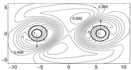
FIG. 3.: Contour plot of the conformal factor $\phi$. The inner thick lines limit the “inner” region where the initial value $\phi=1$ is preserved. The outer thick lines show the apparent horizons and the arrows the direction of the boosts.

TABLE I.: Maximum ($l_{\infty}$) and average of the absolute values ($l_{1}$) of the conformal factor $\phi$ and vector potential $w^{i}$ on the grid volume.

	$\phi$	$w^{x}$	$w^{y}$	$w^{z}$
$l_{\infty}$	$1.009e+0$	$0.462e-2$	$0.168e-1$	$0.421e-2$
$l_{1}$	$0.997e+0$	$0.745e-3$	$0.146e-2$	$0.452e-3$

REFERENCES

- [1] Covariant differentiation with respect to () is denoted by (). Spacetime indices will be denoted by Greek letters and spatial indices by Latin letters.
- [2] G. B. Cook, To appear in “Living Reviews in Relativity” (2000) [gr-qc/0007085].
- [3] G. B. Cook, M. W. Choptuik, M. R. Dubal, S. Klasky, R. A. Matzner and S. R. Oliveira, Phys. Rev. D47, 1471 (1993). G. B. Cook, Phys. Rev. D50, 5025 (1994) [gr-qc/9404043]. T. W. Baumgarte, Phys. Rev. D62, 024018 (2000) [gr-qc/0004050].
- [4] H. P. Pfeiffer, S. A. Teukolsky and G. B. Cook, Phys. Rev. D62, 104018 (2000) [gr-qc/0006084].
- [5] A. D. Kulkarni, L. C. Shepley and J. W. York Jr. Phys. Lett. 96A, 228 (1983).
- [6] S. Brandt and B. Brügmann, Phys. Rev. Lett. 78, 3606 (1997) [gr-qc/9703066].
- [7] A. Garat and R. H. Price, Phys. Rev. D61, 124011 (2000) [gr-qc/0002013].
- [8] N. T. Bishop, R. Isaacson, M. Maharaj and J. Winicour, Phys. Rev. D57, 6113 (1998) [gr-qc/9711076].
- [9] R. A. Matzner, M. F. Huq and D. Shoemaker, Phys. Rev. D59, 024015 (1999) [gr-qc/9805023].
- [10] P. Marronetti, M. Huq, P. Laguna, L. Lehner, R. A. Matzner and D. Shoemaker, Phys. Rev. D62, 024017 (2000) [gr-qc/0001077].
- [11] J. W. York and T. Piran “The Initial Value Problem and Beyond”, Spacetime and Geometry: The Alfred Schild Lectures, R. A. Matzner and L. C. Shepley Eds. University of Texas Press, Austin, Texas. (1982); G. B. Cook, “Initial Data for the Two-Body Problem of General Relativity”, Ph.D. Dissertation, The University of North Carolina at Chapel Hill (1990).
- [12] P. Marronetti, G. J. Mathews and J. R. Wilson, Phys. Rev. D58, 107503 (1998) [gr-qc/9803093]. P. Marronetti, G. J. Mathews and J. R. Wilson, Proceedings of 19th Texas Symposium on Relativistic Astrophysics: Texas in Paris, Paris, France. J. Paul, T. Montmerle, and E. Aubourg Eds. Nuclear Physics B, Proc. Suppl. 80 (2000). [gr-qc/9903105]. P. Marronetti, G. J. Mathews and J. R. Wilson, Phys. Rev. D60, 087301 (1999) [gr-qc/9906088].
- [13] In the numerical implementation of the solver, the terms on the rhs. of Eqs. (13) that include the background affine connection coefficients are passed to the sources. These terms still have the “singularity” embedded in them, thus part of the singular behavior remains. Fortunately, the numerical experiments showed that their influence in the convergence of the algorithm is very small and confined to the points closest to the inner region limit.
- [14] S. Brandt et al., to appear in Phys. Rev. Lett., [gr-qc/0009047].
- [15] If the Ricci scalar exceeds a given threshold value , then the grid point is inside the “inner” region. For this particular hyperbolic encounter, we used .
- [16] The numerical code uses domain decomposition to split the grid in eighteen cubes. The elliptic equations are solved independently in each cube and then the new field values are used to update the source terms of the equations and the boundaries of each cube for the next iteration step. The cubes overlap each other with one buffer grid point that allows the calculation of the cube-surface boundary values. While this scheme worked remarkably well in the case of neutron-star binaries [12], it seems somewhat inadequate for the present case; the convergence is degraded to first order for the grid points adjacent to the cube’s sides. Here, we concentrated on the study of the convergence near the singularities to better test the attenuation method. Since these regions are well inside the center grid cube, they do not present this problem and allowed us to observed the second order convergence clearly. This problem could be solved by increasing the number of overlapping buffer zones or discarding the grid decomposition altogether (working with only one grid), and it will be addressed in future versions of the code.
- [17] M. F. Huq, M. W. Choptuik and R. A. Matzner, gr-qc/0002076.
- [18] P. Marronetti and R. A. Matzner, To appear in the Proceedings of 9th Marcel Grossman Meeting. Rome, Italy, (2000).