Black Holes and Naked Singularities in Low Energy Limit of String Gravity with Modulus Field

Abstract

We show that the black hole solutions of the effective string theory action, where one-loop effects that couple the moduli to gravity via a Gauss-Bonnet term are taken into account, admit primary scalar hair. The requirement of absence of naked singularities imposes an upper bound on the scalar charges.

• ¹ Sternberg Astronomical Institute, Moscow State University,
  Universitetskii Prospect, 13, Moscow 119899, Russia;
  ² Dipartimento di Matematica, Università di Cagliari,
  viale Merello 92, 09123, Cagliari, Italy;
  ³ INFN, Sezione di Cagliari.

1 Introduction

General Relativity describes very well gravity at the classical level, but a quantum theory of gravity requires the introduction of a more general framework. One of the most promising candidates is presently string theory. This theory is believed to change drastically the short-range behavior of classical gravity, but also some of its global properties can be modified, such as black hole thermodynamics. For example, the study of the black hole solutions of effective low-energy theory has shown that, due to the presence of non-minimal couplings, non-trivial scalar hair can arise [1], in contrast with classical general relativity, where no-hair theorems [2] rule out this possibility.

The effects of string theory on gravitational physics are usually investigated by means of effective field theory actions, obtained through a perturbative expansion in the string tension $\alpha$. At the tree level, the effective action of the heterotic (but also other types of) string contains a coupling of the dilaton with gravity via the Gauss-Bonnet term. The black hole solutions of this model have been extensively studied in the literature, both in a perturbative [3] and numerical [4, 5] approach. It turns out that the model admits asymptotically flat black hole solutions with non-trivial dilatonic hair. The scalar charge is not an independent parameter, but is a function of the mass of the black hole, and is therefore an example of secondary hair [6]. Also the thermodynamics is different from that of Schwarzschild black holes. In particular, it was shown that the theory predicts a lower bound on the mass of Gauss-Bonnet black holes [4, 5], which corresponds to the state of highest (but finite) temperature and lowest entropy. The configuration of minimal mass should be identified with the ground state of the Hawking evaporation process.

In order to build realistic models, one should however take into account that in string theory other scalar fields are present in the spectrum in addition to the dilaton, as for example the moduli, which originate from the compactification of the higher-dimensional spacetime. These also couple to gravity through one-loop effects. At leading order the coupling term is proportional to the logarithm of a Dedekind $\eta$-function of the moduli, which multiplies the Gauss-Bonnet term [7]. The effect of the non-minimal coupling of the moduli to gravity in a cosmological context has been studied in several papers [8] and it has been shown that in some cases it may lead to models without initial singularities, but to our knowledge no investigation has been devoted till now to its implications on black hole physics.

On the other hand, it is well known that in effective string actions the electromagnetic field exhibits a non-minimal coupling to the dilaton and the moduli similar to that of the Gauss-Bonnet term [9]. The black hole solutions have been thoroughly studied in this case: if one neglects the moduli, one obtains exact magnetically charged solutions, with secondary scalar hair, the scalar charge being a function of the mass and the magnetic charge [1]. If one instead takes into account also one modulus, the general solution can no longer be written in analytic form, but it can nevertheless be shown to depend on three parameters [10]: thus in this case a new independent parameter arises, besides the mass and the charge, and one may speak of a primary scalar hair.

In this paper, we investigate if a similar phenomenon can occur in the purely gravitational sector. Since we are mainly interested in showing the existence of primary scalar hair in the scalar-gravity sector, we consider a simplified model with a dilaton and a unique modulus which couples exponentially with the Gauss-Bonnet term. We study it both in a perturbative and numerical setting using the techniques developed in Ref. [3] and [4], respectively. We find that in fact the qualitative features are similar to the case of Maxwell coupling. We also find that an upper limit must be imposed on the scalar charges for given mass, in order to avoid naked singularities. This is reminiscent of the extremality bounds in the multiscalar Einstein-Maxwell case [13].

The structure of our paper is the following. In section 2 we present the perturbative solution and discuss its thermodynamical properties. In section 3 we describe the numerical solution and the occurrence of an upper bound for the scalar charges. Section 4 contains a discussion and the main conclusions.

2 Perturbative Solution

The bosonic sector of the effective action for the heterotic string in absence of Yang-Mills and axionic fields, is given at leading order in $\alpha^{\prime}$ by

$$I_{eff}={1\over 16\pi}\int d^{4}x\sqrt{-g}\left[{\cal R}-2(\nabla\Phi)^{2}-2(\nabla\Sigma)^{2}+\alpha({\rm e}^{-2\Phi}+\delta{\rm e}^{-2\Sigma}){\cal S}\right]$$ (1)

where $\alpha\equiv\alpha^{\prime}/8$, $\delta$ is a coupling constant of order unity, $\Phi$ is the dilaton, $\Sigma$ is a modulus, whose coupling with the Gauss-Bonnet term, ${\cal S}\equiv{\cal R}_{mnpq}{\cal R}^{mnpq}-4{\cal R}_{mn}{\cal R}^{mn}+{\cal R}^{2}$ has been taken for simplicity to be of exponential form. The field equations equations can be written as

$$G_{mn}=T_{mn}^{(\Phi)}+T_{mn}^{(\Sigma)},$$

$$\nabla^{2}\Phi={\alpha\over 2}{\rm e}^{-2\Phi}{\cal S},\hskip 25.0pt\hskip 25.0pt\nabla^{2}\Sigma={\alpha\delta\over 2}{\rm e}^{-2\Sigma}{\cal S},$$ (2)

where

$$T_{mn}^{(\Phi)}=4\alpha{\rm e}^{-2\Phi}\Big{[}4{\cal R}_{p(m}\nabla_{n)}\nabla_{p}\Phi-2{\cal R}_{mn}\nabla_{p}\nabla_{p}\Phi-{\cal R}\nabla_{m}\nabla_{n}\Phi-2{\cal R}_{qmnp}\nabla_{p}\nabla_{q}\Phi\Big{]}$$ (3)

$$-8\alpha{\rm e}^{-2\Phi}\Big{[}4{\cal R}_{p(m}\nabla_{n)}\Phi\nabla_{p}\Phi-2{\cal R}_{mn}\nabla_{p}\Phi\nabla_{p}\Phi-{\cal R}\nabla_{m}\Phi\nabla_{n}\Phi-2{\cal R}_{qmnp}\nabla_{p}\Phi\nabla_{q}\Phi\Big{]}$$

$$+2\nabla_{m}\Phi\nabla_{n}\Phi-g_{mn}\nabla_{m}\Phi\nabla_{n}\Phi,$$

and an alougous expression for $T_{mn}^{(\Sigma)}$. The total energy-momentum is conserved but, as noticed in [5] for the case of a single scalar, its time component, corresponding to the total energy, is not positive definite, due to the contribution of the Gauss-Bonnet term, leaving room for the possibility of a violation of the no-hair conjecture.

We look for spherically symmetric solutions, with scalars $\Phi=\Phi(r)$, $\Sigma=\Sigma(r)$. A generic spherically symmetric metric can be written as

$$ds^{2}=-\Delta(r)dt^{2}+{\sigma^{2}(r)\over\Delta(r)}dr^{2}+R^{2}(r)d\Omega^{2}.$$ (4)

Instead of substituting the ansatz (4) into the field equations (2), it is easier to substitute it directly into the action, and then vary with respect to the fields $\Phi$, $\Sigma$, $\Delta$, $\sigma$ and $R$.

The action reads:

$$I={1\over 16\pi}\int d^{4}x{2\over\sigma}\Big{[}\Delta^{\prime}RR^{\prime}+\Delta R^{\prime 2}+\sigma^{2}-R^{2}\Delta(\Phi^{\prime 2}+\Sigma^{\prime 2})$$ (5)

$$-2\alpha({\rm e}^{-2\Phi}+\delta{\rm e}^{-2\Sigma})^{\prime}\Delta^{\prime}\left(1-\sigma^{-2}\Delta R^{\prime 2}\right)\Big{]}$$

The field equations can then be written in the form:

$$(\sigma^{-1}\Delta R^{2}\Phi^{\prime})^{\prime}=-2\alpha{\rm e}^{-2\Phi}[(\sigma^{-1}\Delta^{\prime}(1-\sigma^{-2}\Delta R^{\prime 2})]^{\prime},$$

$$(\sigma^{-1}\Delta R^{2}\Sigma^{\prime})^{\prime}=-2\alpha\delta{\rm e}^{-2\Sigma}[(\sigma^{-1}\Delta^{\prime}(1-\sigma^{-2}\Delta R^{\prime 2})]^{\prime},$$

$$RR^{\prime\prime}-\sigma^{-1}\sigma^{\prime}RR^{\prime}=2\alpha\sigma^{-1}V^{\prime}[2\sigma^{-1}\Delta R^{\prime}R^{\prime\prime}-(1-3\sigma^{-2}\Delta R^{\prime 2})]$$ (6)

$$-2\alpha V^{\prime\prime}\sigma^{-1}(1-\sigma^{-2}\Delta R^{\prime 2})-R^{2}(\Phi^{\prime 2}+\Sigma^{\prime 2}),$$

$$\Delta^{\prime}RR^{\prime}+\Delta R^{\prime 2}-\sigma^{-2}=-2\alpha V^{\prime}\Delta^{\prime}(1-3\sigma^{-2}\Delta R^{\prime 2})+\Delta R^{2}(\Phi^{\prime 2}+\Sigma^{\prime 2}),$$

$$\Delta^{\prime\prime}R+2\Delta^{\prime}R^{\prime}+2\Delta R^{\prime\prime}-\sigma^{-1}\sigma^{\prime}(\Delta^{\prime}R+2\Delta R^{\prime})$$

$$=4\alpha V^{\prime}(\sigma^{-3}\Delta\Delta^{\prime}R^{\prime})^{\prime}+4\alpha V^{\prime\prime}\sigma^{-3}\Delta\Delta^{\prime}R^{\prime}-2R\Delta(\Phi^{\prime 2}+\Sigma^{\prime 2}),$$

where $V=({\rm e}^{-2\Phi}+\delta{\rm e}^{-2\Sigma})$ and a prime denotes derivative with respect to $r$. Only four of the previous equations are independent.

In order to find approximate solutions to the field equations, we adopt the approach of Ref. [3] and expand the fields around the background constituted by the Schwarzschild metric with vanishing scalar fields, which is of course a solution for $\alpha=0$. Our expansion is in the parameter $\alpha/m^{2}$, $m$ being the mass of the background Schwarzschild solution. Since $\alpha$ is believed to be of order unity in Planck units, the expansion is valid for large $m$, in the region where $\alpha{\cal S}\ll{\cal R}$, i. e. for $r^{3}\gg\alpha m$. For macroscopic black holes ($m\gg 1$) this condition is always satisfied, except in a neighborhood of the singularity, well inside the horizon (region of strong curvature). In particular, the approximation is valid for the discussion of the asymptotic properties of the fields, and the questions concerning the scalar hair. Near the physical singularity, however, the higher order corrections to the effective string lagrangian become important and the perturbation theory is no longer reliable. We shall however discuss this regime using numerical techniques in the next section.

At this point, it must be observed that the ansatz (4) for the metric is too general and still leaves the possibility of a choice of gauge. In order to perform the perturbative calculations, the most convenient choice [3] is to impose $\sigma\equiv 1$, i.e.

$$ds^{2}=-\Delta(r)dt^{2}+{1\over\Delta(r)}dr^{2}+R^{2}(r)d\Omega^{2}.$$ (7)

This gauge was also used for finding exact charged black hole solutions in effective string theory [1].

We expand the fields as follows:

$$\Delta = \Delta_{0}(1+\alpha\psi_{1}+\alpha^{2}\psi_{2}+\alpha^{3}\psi_{3}+\dots),$$

$$R = r+\alpha\rho_{1}+\alpha^{2}\rho_{2}+\alpha^{3}\rho_{3}+\dots,$$

$$\Phi = \alpha\Phi_{1}+\alpha^{2}\Phi_{2}+\alpha^{3}\Phi_{3}+\dots,$$

$$\Sigma = \Sigma_{0}+\alpha\Sigma_{1}+\alpha^{2}\Sigma_{2}+\alpha^{3}\Sigma_{3}+\dots,$$ (8)

where $\Delta_{0}=(1-2m/r)$. We have normalized $\Phi$ such that $\Phi\to 0$ at infinity. This is always possible, by rescaling the coupling constant $\alpha$ (this means that our expansion is actually in $\alpha{\rm e}^{-2\Phi_{0}}$). However, it is not possible to rescale independently also $\Sigma$, and hence we take $\Sigma\to\Sigma_{0}$ at infinity. The parameters $\delta$ and $\Sigma_{0}$ will always appear in the combination $Z=\delta{\rm e}^{-2\Sigma_{0}}$.

Substituting the expansion (2) into the field equations (2), one obtains at first order

$$[r(r-2m)\Phi_{1}^{\prime}]^{\prime}={24m^{2}\over r^{4}},\hskip 25.0pt[r(r-2m)\Sigma_{1}^{\prime}]^{\prime}={24m^{2}Z\over r^{4}}.$$ (9)

With the previous boundary conditions , requiring regularity at the horizon $r=2m$, the scalar fields are uniquely determined at first order:

$$\Phi_{1}={\Sigma_{1}\over Z}=-{1\over m}\left({1\over r}+{m\over r^{2}}+{4m^{2}\over 3r^{3}}\right),$$ (10)

The equations for the metric fields are given at the same order by

$$\rho_{1}^{\prime\prime}=0,\hskip 25.0pt\hskip 25.0pt[(r-2m)\psi_{1}]^{\prime}=-{2m\over r^{2}}\rho_{1}.$$ (11)

We impose the boundary conditions that $\rho_{1}\to$ const, $\psi_{1}\to 0$ at infinity. We are still free to choose the boundary conditions at $r=2m$. Changing the boundary conditions at $r=2m$ yields a reparametrization of the solutions, but no change in their physical properties: in particular, the relations between the physical quantities, like mass, temperature and entropy, are independent of the parametrization. The most convenient choice is to require that the $\rho_{i}$ and $\psi_{i}$ are regular at $r=2m$. This is equivalent to fix the location of the horizon at $r=2m$. With these boundary conditions, $\rho_{1}=0$, $\psi_{1}=0$. This choice greatly simplifies the higher order calculations.

We can now evaluate the second order corrections. With the stated boundary conditions, the equations for the second order perturbations give

$$[r(r-2m)\Phi_{2}^{\prime}]^{\prime}=-{48m^{2}\over r^{4}}\Phi_{1},$$

$$[r(r-2m)\Sigma_{2}^{\prime}]^{\prime}=-{48Zm^{2}\over r^{4}}\Sigma_{1},$$

$$\rho_{2}^{\prime\prime}=-r(\Phi_{1}^{\prime 2}+\Sigma_{1}^{\prime 2})+{8m\over r^{2}}(\Phi_{1}^{\prime\prime}+Z\Sigma_{1}^{\prime\prime}),$$ (12)

$$[(r-2m)\psi_{2}]^{\prime}=-(r-2m)\rho_{2}^{\prime\prime}-2{r-m\over r}\rho_{2}^{\prime}-{2m\over r^{2}}\rho_{2}$$

$$+8m{r-2m\over r^{2}}(\Phi_{1}^{\prime\prime}+Z\Sigma_{1}^{\prime\prime})-16m{r-3m\over r^{3}}(\Phi_{1}^{\prime}+Z\Sigma_{1}^{\prime}),$$

whose solution is

$$\Phi_{2}={\Sigma_{2}\over Z^{2}}=-{1\over m^{3}}\left({73\over 60r}+{73m\over 60r^{2}}+{73m^{2}\over 45r^{3}}+{73m^{3}\over 30r^{4}}+{112m^{4}\over 75r^{5}}+{8m^{5}\over 9r^{6}}\right),$$

$$\rho_{2}=-{1+Z^{2}\over m^{2}}\left({1\over 2r}+{2m\over 3r^{2}}+{7m^{2}\over 3r^{3}}+{16m^{3}\over 5r^{4}}+{24m^{4}\over 5r^{5}}\right),$$

$$\psi_{2}=-{1+Z^{2}\over m^{3}}\left({1\over 6r}+{m\over 3r^{2}}+{4m^{2}\over 3r^{3}}-{14m^{3}\over 3r^{4}}-{136m^{4}\over 15r^{5}}-{272m^{5}\over 15r^{6}}\right).$$

Up to this order, $\Phi$ and $\Sigma$ are proportional in this gauge. However, in order to clarify the structure of the solutions, it is useful to go to the next order, even if such corrections would of course be modified by taking into account terms of order $\alpha^{2}$ in the action. A long but straightforward calculation gives

$$\rho_{3}=-{73\,(1+Z^{3})\over{60\,{m^{4}}\,r}}+o\left({1\over r^{2}}\right),\hskip 25.0pt\psi_{3}=-{73\,(1+Z^{3})\over{180\,{m^{5}}\,r}}+o\left({1\over r^{2}}\right),$$

$$\Phi_{3}=-{16480+3969\,Z^{2}\over{7560\,{m^{5}}\,r}}+o\left({1\over r^{2}}\right),\hskip 25.0pt\Sigma_{3}=-{Z\,(3969+16480\,Z^{2})\over{7560\,{m^{5}}\,r}}+o\left({1\over r^{2}}\right).$$

From these results appears that the metric functions are expanded in terms of $\alpha^{k}(1+Z)^{k}$, while the scalar fields depend in a more involved way from the parameters. Moreover, the functional dependences of the dilaton and the modulus on $r$ are different if $Z\neq 1$.

The perturbative solutions have the following properties: a horizon is present at $r=2m$, while a singularity is located at the zero of $R$; the evaluation of this zero is however outside the range of validity of our approximation. It can be expected nevertheless that for small values of the mass, or great values of $Z$, the zero can occur for $r>2m$, leading to the presence of naked singularities. This will be confirmed by the numerical results of next section.

The mass $M$ of the black hole can be deduced from the asymptotic behavior of the metric function $\Delta$ and is given by

$$M=m\left(1+{1\over 12}{\alpha^{2}(1+Z^{2})\over m^{4}}+{73\over 360}{\alpha^{3}(1+Z^{3})\over m^{6}}\right).$$ (13)

Its value is greater than that of the Schwarzschild black hole with equal radius. Analogously, from the asymptotic behaviour of $\Phi$ and $\Sigma$ one can deduce the scalar charges $D_{\Phi}$ and $D_{\Sigma}$, which, in terms of the mass $M$, turn out to be

$$D_{\Phi}={\alpha\over M}\left(1+{73\over 60}{\alpha\over M^{2}}+{17110+4599Z^{2}\over 7560}{\alpha^{2}\over M^{4}}\right),$$

$$D_{\Sigma}={\alpha Z\over M}\left(1+{73\over 60}{\alpha Z\over M^{2}}+{4599+17110Z^{2}\over 7560}{\alpha^{2}\over M^{4}}\right).$$ (14)

It is clear that, contrary to the case in which only one scalar field is present [3], the scalar charges are no longer function only of the mass of the black hole, but depend also on another parameter, which we identify with $Z$. Hence, in analogy with the dilaton-modulus gravity non-minimally coupled to the electromagnetic field [10], also in this case a primary scalar hair is present in the solution. This gives an example of primary scalar hair in pure gravity models. We notice that, at leading order, $Z\sim D_{\Sigma}/D_{\Phi}$.

The temperature of the black hole can be defined as usual as the inverse periodicity of the time coordinate which renders regular the Euclidean section of the metric. This is given by [11]

$$T={1\over 4\pi\sqrt{g_{00}g_{11}}}{dg_{00}\over dr}\Bigl{\arrowvert}_{\rm hor}\,,$$

which yields, at order $\alpha^{3}$:

$$T={1\over 8\pi m}\big{(}1+\alpha^{2}\psi_{2}(2m)+\alpha^{3}\psi_{3}(2m)\big{)}.$$

Taking into account (13), a straightforward calculation leads to

$$T={1\over 8\pi M}\left(1+{73\over 120}{\alpha^{2}(1+Z^{2})\over M^{4}}+{12511\over 7560}{\alpha^{3}(1+Z^{3})\over M^{6}}\right).$$

The temperature is higher than that of a Schwarzschild black hole of equal mass, but is still a monotonically decreasing function of the mass.

The entropy $S$ can be defined by means of the Euclidean formalism [12] as

$$S=\beta{\partial I_{E}\over\partial\beta}-I_{E},$$ (15)

where $\beta$ is the inverse temperature and $I_{E}$ the Euclidean action

$$I_{E} = -{1\over 16\pi}\int_{M}[{\cal R}-2(\nabla\Phi)^{2}-2(\nabla\Sigma)^{2}+\alpha\ ({\rm e}^{-2\Phi}+\delta{\rm e}^{-2\Sigma}){\cal S})]dV$$ (16)

$$-{1\over 8\pi}\int_{\partial M}(K-K_{0})d\Sigma$$

where $K$ is the exterior curvature. A lenghty calculation gives

$$S=4\pi M^{2}\left(1+{73\over 120}{\alpha^{2}(1+Z^{2})\over M^{4}}+{12511\over 15120}{\alpha^{3}(1+Z^{3})\over M^{6}}\right).$$

In the range of validity of our approximation, the thermodynamical quantities of course do not differ much from their background values, except that now they depend on the further parameter $Z$. They behave differently only for $M\ll\alpha$, where however the approximation breaks down. It is interesting to notice that all the thermodynamical quantities are expanded in terms of $\alpha^{k}(1+Z^{k})$.

3 Numerical Solution and Naked Singularity

As discussed previously, the perturbative solution is not valid in the whole domain of definition of the solution. Since we are not able to find the exact analytical solution of the field equations, we use the numerical approach described in Ref. [4]. For this calculation it is more convenient to choose a gauge in which the metric function $R$ is identified with the radial coordinate $r$, i.e.

$$ds^{2}=-\Delta dt^{2}+\frac{\sigma^{2}}{\Delta}dR^{2}+R^{2}d\Omega^{2},$$

where $\Delta=\Delta(R)$, $\sigma=\sigma(R)$. Comparison with (4) yields $\sigma(R)=dr/dR$. Of course, the physical quantities do not depend on the choice of gauge. However, in order to make the comparison of results easier, we give the perturbative expansions in the new coordinates:

$$\Delta(R)=(1-2m/R)(1+\alpha^{2}\psi_{2}(R)+\alpha^{3}\psi_{3}(R))+(2m/R^{2})(\alpha^{2}\rho_{2}(R)+\alpha^{3}\rho_{3}(R))+\dots$$

$$\sigma(R)=1-\alpha^{2}\rho_{2}^{\prime}(R)-\alpha^{3}\rho_{3}^{\prime}(R)+\dots$$

$$\Phi(R)=\Phi_{0}+\alpha\Phi_{1}(R)+\alpha^{2}\Phi_{2}(R)+\alpha^{3}(\Phi_{3}(R)-\Phi_{1}^{\prime}(R)\rho_{2}(R))+\dots$$

$$\Sigma(R)=\Sigma_{0}+\alpha\Sigma_{1}(R)+\alpha^{2}\Sigma_{2}(R)+\alpha^{3}(\Sigma_{3}(R)-\Sigma_{1}^{\prime}(R)\rho_{2}(R))+\dots$$

where use has been made of the condition $\psi_{1}=\rho_{1}=0$, and the functions $\rho_{i}$, $\psi_{i}$  $\Phi_{i}$ and $\Sigma_{i}$ are those obtained above, evaluated at $r=R$. In particular, the metric function are, up to order $\alpha^{2}$,

$$\Delta = 1-{2m\over R}-{\alpha^{2}(1+Z^{2})\over m^{4}}\left({m\over 6R}+{5m^{3}\over 3R^{3}}-{6m^{4}\over R^{4}}+{74m^{5}\over 15R^{5}}+{32m^{6}\over 5R^{6}}+{688m^{7}\over 15R^{7}}\right)$$

$$\sigma = 1-{\alpha^{2}(1+Z^{2})\over m^{4}}\left({m^{2}\over 2R^{2}}+{4m^{3}\over 3R^{3}}+{7m^{4}\over R^{4}}+{64m^{5}\over 5R^{5}}+{24m^{6}\over R^{6}}\right)$$

In the parametrization (3) the Einstein-Lagrange equations can be written in a matrix form (we set all the string coupling constants to be equal to one for simplicity)

$$a_{i1}\Delta^{\prime\prime}+a_{i2}\sigma^{\prime}+a_{i3}\Phi^{\prime\prime}+a_{i4}\Sigma^{\prime\prime}=b_{i},$$ (17)

where $i=1,\ldots,4$ and the entries of the matrices $a_{ij}$ and $b_{i}$ are

$$a_{11} = 0$$

$$a_{12} = -\sigma^{2}R+4(\sigma^{2}-3\Delta)(e^{-2\Phi}\Phi^{\prime}+e^{-2\Sigma}\Sigma^{\prime})$$

$$a_{13} = 4\sigma(\Delta-\sigma^{2})e^{-2\Phi}$$

$$a_{14} = 4\sigma(\Delta-\sigma^{2})e^{-2\Sigma}$$

$$a_{21} = \sigma^{3}R+8\Delta\sigma(e^{-2\Phi}\Phi^{\prime}+e^{-2\Sigma}\Sigma^{\prime})$$

$$a_{22} = -\sigma^{2}(\Delta^{\prime}R+2\Delta)-24\Delta\Delta^{\prime}(e^{-2\Phi}\Phi^{\prime}+e^{-2\Sigma}\Sigma^{\prime})$$

$$a_{23} = 8\Delta\Delta^{\prime}\sigma e^{-2\Phi}$$

$$a_{24} = 8\Delta\Delta^{\prime}\sigma e^{-2\Sigma}$$

$$a_{31} = 4e^{-2\Phi}\sigma(\Delta-\sigma^{2})$$

$$a_{32} = 2\sigma^{2}R^{2}\Delta\Phi^{\prime}-4e^{-2\Phi}\Delta^{\prime}(3\Delta-\sigma^{2})$$

$$a_{33} = -2\sigma^{3}R^{2}\Delta$$

$$a_{34} = 0$$

$$a_{41} = 4e^{-2\Sigma}\sigma(\Delta-\sigma^{2})$$

$$a_{42} = 2\sigma^{2}R^{2}\Delta\Sigma^{\prime}-4e^{-2\Sigma}\Delta^{\prime}(3\Delta-\sigma^{2})$$

$$a_{43} = 0$$

$$a_{44} = -2\sigma^{3}R^{2}\Delta$$

$$b_{1} = -\sigma^{3}R^{2}(\Phi^{\prime 2}+\Sigma^{\prime 2})+8\sigma(\Delta-\sigma^{2})(e^{-2\Phi}\Phi^{\prime 2}+e^{-2\Sigma}\Sigma^{\prime 2})$$

$$b_{2} = -2\sigma^{3}(\Delta^{\prime}+\Delta R(\Phi^{\prime 2}+\Sigma^{\prime 2}))+16\Delta\Delta^{\prime}\sigma(e^{-2\Phi}\Phi^{\prime 2}+e^{-2\Sigma}\Sigma^{\prime 2})$$

$$- 8\Delta^{\prime 2}\sigma(e^{-2\Phi}\Phi^{\prime}+e^{-2\Sigma}\Sigma^{\prime})$$

$$b_{3} = 2\sigma^{3}R\Phi^{\prime}(\Delta^{\prime}R+2\Delta)-4e^{-2\Phi}\Delta^{\prime 2}\sigma$$

$$b_{4} = 2\sigma^{3}R\Sigma^{\prime}(\Delta^{\prime}R+2\Delta)-4e^{-2\Sigma}\Delta^{\prime 2}\sigma$$

The last (constraint) equation is

$$\sigma^{2}\biggl{[}\Delta R^{2}(\Phi^{\prime 2}+\Sigma^{\prime 2})+\sigma^{2}-\Delta^{\prime}R-\Delta\biggr{]}$$

$$+ 4\biggl{[}\lambda_{\Phi}e^{-2\Phi}\Phi^{\prime}+\lambda_{\Sigma}qe^{-2q\Sigma}\Sigma^{\prime}\biggr{]}\Delta^{\prime}(\sigma^{2}-3\Delta)=0$$

The numerical integration is performed as follows: we start from a neighborood of the horizon and integrate towards infinity. The mass and charges of the solution are then evaluated from the asymptotic behaviour of the metric functions and the integration is performed again backwards. More technical details on the numerical procedure can be found in [4].

The behaviour of the solution outside the horizon agrees with that obtained by perturbative methods in the previous section (see Figures 1-4) and is similar to that of the single-scalar solutions discussed in [3, 4, 5]. When $D_{\Sigma}$ vanishes, we recover the solutions described in Ref. [4]. In particular, one must impose a lower bound on the black hole mass in order to avoid the occurrence of naked singularities. For non-zero value of $D_{\Sigma}$ the situation changes significantly. Taking $M$ and $D_{\Phi}$ fixed, for small values of $D_{\Sigma}$ the behavior of the solution does not differ much from the case of a single scalar field, except that the position of the inner black hole singularity slowly moves up. This situation is shown by the solid lines in Figs.1-4, where the dependence of the functions $\Delta$, $\sigma$, $e^{-2\Phi}$ and $e^{-2\Sigma}$ against the radial coordinate $r$ is plotted. When $D_{\Sigma}$ reaches a critical value ${D_{\Sigma}}_{crit}$ the positions of the singularity $R_{s}$ and the horizon $R_{h}$ coincide. The dependence of ${D_{\Sigma}}_{crit}$ against black hole mass is represented on Figure 5. When $D_{\Sigma}>{D_{\Sigma}}_{crit}$ a naked singularity appears. This situation is shown by dashed lines in Figs. 1-4. This naked singularity is a continuation of the black hole inner singularity and has the same nature. Of course, since the system is symmetric for the exchange of $\Phi$ and $\Sigma$, an analogous behavior is expected when $\Phi$ is varied and $\Sigma$ held fixed. The dependence of ${D_{\Sigma}}_{crit}$ from the black hole mass $M$ is approximately linear. Hence, according to the cosmic censorship conjecture, the mass of the black hole gives an upper limit for the modulus/dilatonic field charge.

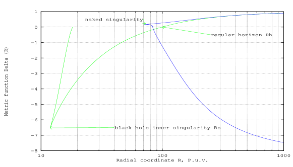
Figure 1: Dependence of the metric function $\Delta$ against the radial coordinate $R$, Planck unit values, when $D_{\Sigma}\ll{D_{\Sigma}}_{crit}$ (thin line) and $D_{\Sigma}\gg{D_{\Sigma}}_{crit}$ (thick line).

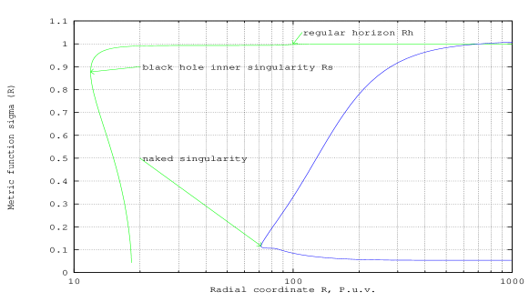
Figure 2: Dependence of the metric function $\sigma$ against the radial coordinate $R$, Planck unit values, when $D_{\Sigma}\ll{D_{\Sigma}}_{crit}$ (thin line) and $D_{\Sigma}\gg{D_{\Sigma}}_{crit}$ (thick line)

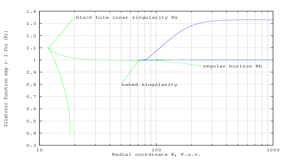
Figure 3: Dependence of the dilatonic function $e^{-2\Phi}$ against the radial coordinate $R$, Planck unit values, when $D_{\Sigma}\ll{D_{\Sigma}}_{crit}$ (thin line) and $D_{\Sigma}\gg{D_{\Sigma}}_{crit}$ (thick line)

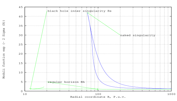
Figure 4: Dependence of the modulus function $e^{-2\Sigma}$ against the radial coordinate $R$ when $D_{\Sigma}\ll{D_{\Sigma}}_{crit}$ (thin line) and $D_{\Sigma}\gg{D_{\Sigma}}_{crit}$ (thick line)

From a mathematical point of view the appearance of this singularity is a consequence of the vanishing of the second factor (in brackets) of the determinant $D_{main}$ of the system (17)

$$D_{main} = \Delta^{2}\biggl{[}A\Delta^{2}+B\Delta+C\biggr{]},\hskip 25.0pt\mbox{where}$$

$$A = 64r^{2}\sigma^{5}\biggl{[}4r^{2}\sigma^{2}e^{-4\Phi}\Phi^{\prime 2}+8r^{2}\sigma^{2}e^{-2\Phi}\Phi^{\prime}e^{-2\Sigma}\Sigma^{\prime}+4r^{2}\sigma^{2}e^{-4\Sigma}\Sigma^{\prime 2}$$

$$- \sigma^{2}e^{-4\Phi}-\sigma^{2}e^{-4\Sigma}+12e^{-6\Phi}\Phi^{\prime}\Delta^{\prime}+12e^{-4\Phi}e^{-2\Sigma}\Sigma^{\prime}\Delta^{\prime}$$

$$+ 12e^{-2\Phi}\Phi^{\prime}e^{-4\Sigma}\Delta^{\prime}+12e^{-6\Sigma}\Sigma^{\prime}\Delta^{\prime}\biggr{]}$$

$$B = 32r^{2}\sigma^{6}\biggl{[}r^{3}\sigma^{3}e^{-2\Phi}\Phi^{\prime}+r^{3}\sigma^{3}e^{-2\Sigma}\Sigma^{\prime}+r^{3}\sigma^{2}e^{-2\Phi}\Phi^{\prime}+r^{3}\sigma^{2}e^{-2\Sigma}\Sigma^{\prime}$$

$$+ 2r\sigma e^{-4\Phi}\Delta^{\prime}+2r\sigma e^{-4\Sigma}\Delta^{\prime}+2re^{-4\Phi}\Delta^{\prime}+2re^{-4\Sigma}\Delta^{\prime}+4\sigma^{3}e^{-4\Phi}$$

$$+ 4\sigma^{3}e^{-4\Sigma}-16\sigma e^{-6\Phi}\Phi^{\prime}\Delta^{\prime}-16\sigma e^{-4\Phi}e^{-2\Sigma}\Sigma^{\prime}\Delta^{\prime}$$

$$- 16\sigma e^{-2\Phi}\Phi^{\prime}e^{-4\Sigma}\Delta^{\prime}-16\sigma e^{-6\Sigma}\Sigma^{\prime}\Delta^{\prime}\biggr{]}$$

$$C = 4r^{2}\sigma^{8}\biggl{[}r^{4}\sigma^{2}-16r\sigma e^{-4\Phi}\Delta^{\prime}-16r\sigma e^{-4\Sigma}\Delta^{\prime}-16re^{-4\Phi}\Delta^{\prime}$$

$$- 16re^{-4\Sigma}\Delta^{\prime}-16\sigma^{3}e^{-4\Phi}-16\sigma^{3}e^{-4\Sigma}-64\sigma e^{-6\Phi}\Phi^{\prime}\Delta^{\prime}$$

$$- 64\sigma e^{-4\Phi}e^{-2\Sigma}\Sigma^{\prime}\Delta^{\prime}-64\sigma e^{-2\Phi}\Phi^{\prime}e^{-4\Sigma}\Delta^{\prime}-64\sigma e^{-6\Sigma}\Sigma^{\prime}\Delta^{\prime}\biggr{]}$$

A naked singularity occurs when the factor in the bracket of $D_{main}$ vanishes before the metric function $\Delta$. Figure 6 represents the dependence of the position of the zero of $D_{main}$ against the parameter $Z$.

Figure 5: The dependence of the critical modulus charge ${D_{\Sigma}}_{crit}$ against the black hole mass $M$ in Planck unit values, for $D_{\Phi}=1$.

Figure 6: The dependence of the value of $R$ for which $D_{main}=0$, against the parameter $Z=D_{\Sigma}/D_{\Phi}$.

The thermodynamical parameters can evaluated numerically and compared with the perturbative results. This is interesting especially in order tounderstand their behaviour for small mass, where the perturbative approach fails. The temperature can be obtained from (2) in a straightforward way. For the calculation of the entropy, eq. (15) has been used. In particular, the Euclidian action $I_{E}$ was evaluated by adding its definition as an additional equation to the main system (17).

The numerical evaluation of the black hole temperature $T$ and entropy $S$ agrees with the perturbative results for great $M$, see the Table 1. A similar agreement holds for the entropy.

Table 1: The dependence of the black hole temperature $T$ against the mass $M$ and the parameter $Z\approx D_{\Sigma}/D_{\Phi}$ for the numerical and perturbative solutions. The agreement is better for great $M$ or small $Z$, in accordance with the limit of validity of the perturbative approach.

$M$	$Z$	$T$ numerical	$T$ perturbative
4.0	0.1	$1.032079\ *\ 10^{-02}$	$9.975080\ *\ 10^{-03}$
	1.0	$1.041815\ *\ 10^{-02}$	$1.000250\ *\ 10^{-02}$
5.0	0.1	$8.094905\ *\ 10^{-03}$	$7.966414\ *\ 10^{-03}$
	1.0	$8.169681\ *\ 10^{-03}$	$7.974924\ *\ 10^{-03}$
	10.0	$1.007615\ *\ 10^{-02}$	$9.583720\ *\ 10^{-03}$
10.0	0.1	$3.977655\ *\ 10^{-03}$	$3.979124\ *\ 10^{-03}$
	1.0	$3.979633\ *\ 10^{-03}$	$3.979371\ *\ 10^{-03}$
	10.0	$4.101194\ *\ 10^{-03}$	$4.009911\ *\ 10^{-03}$
20.0	0.1	$1.986029\ *\ 10^{-03}$	$1.989444\ *\ 10^{-03}$
	1.0	$1.985790\ *\ 10^{-03}$	$1.989452\ *\ 10^{-03}$
	10.0	$1.989498\ *\ 10^{-03}$	$1.990252\ *\ 10^{-03}$
30.0	0.1	$1.323841\ *\ 10^{-03}$	$1.326292\ *\ 10^{-03}$
	1.0	$1.323821\ *\ 10^{-03}$	$1.326293\ *\ 10^{-03}$
	10.0	$1.324732\ *\ 10^{-03}$	$1.326395\ *\ 10^{-03}$
40.0	0.1	$9.931118\ *\ 10^{-04}$	$9.947186\ *\ 10^{-04}$
	1.0	$9.931105\ *\ 10^{-04}$	$9.947189\ *\ 10^{-04}$
	10.0	$9.933026\ *\ 10^{-04}$	$9.947426\ *\ 10^{-04}$
50.0	0.1	$7.943050\ *\ 10^{-04}$	$7.957748\ *\ 10^{-04}$
	1.0	$7.943053\ *\ 10^{-04}$	$7.957749\ *\ 10^{-04}$
	10.0	$7.948299\ *\ 10^{-04}$	$7.957825\ *\ 10^{-04}$

Finally, we notice that the thermodynamical parameters stay finite in the extremal case. The thermodynamics is therefore analogous to that studied in absence of modulus fields [4, 5], except that now one has one further independent parameter (the scalar charge).

4 Discussion and conclusions

We have shown perturbatively the occurrence of primary scalar hair in black hole solutions of models with more than one scalar field non-minimally coupled to gravity via the Gauss-Bonnet term. This result has been checked numerically. From the numerical calculations also follows that naked singularities can appear for small values of the mass (as in pure dilaton-Gauss-Bonnet models), or for large values of the scalar charges. This is a novel feature of the model under study, and can be compared with a similar phenomenon occurring in multi-scalar Einstein-Maxwell models [13]. In that case some analytical relations for the extremality condition of the black holes can be obtained, while in our case this seems not to be possible. We can however conjecture that a relation of the same kind exists also in our case.

References

References

• [1] D. Garfinkle, G.T. Horowitz, and A. Strominger, Phys. Rev. D 43, 3140 (1991).
• [2] J.D. Bekenstein, Phys. Rev. D 5, 1239 (1972); J.E. Chase, Comm. Math. Phys. 19, 276 (1970).
• [3] S. Mignemi and N.R. Stewart, Phys. Rev. D 47, 5259 (1993).
• [4] S.O. Alexeyev and M.V. Pomazanov, Phys. Rev. D 55, 2110 (1997); S.O. Alexeyev and M.V. Sazhin, Gen. Relativ. and Grav. 8, 1187 (1998).
• [5] P. Kanti, N.E. Mavromatos, J. Rizos, K. Tamvakis and E. Winstanley, Phys. Rev. D 54, 5049 (1996); P. Kanti and K. Tamvakis, Phys. Lett. B 392, 30 (1997); T. Torii, H. Yajima, and K. Maeda, Phys. Rev. D 55, 739 (1997).
• [6] S. Coleman, J. Preskill, and F. Wilczek, Nucl. Phys. B380, 447 (1992).
• [7] I. Antoniadis, J. Rizos, and K. Tamvakis, Nucl. Phys. B415, 497 (1994).
• [8] R. Easther and K. Maeda, Phys. Rev. D 54, 7252 (1996); P. Kanti, J. Rizos, and K. Tamvakis, Phys. Rev. D 59, 083512 (1999); S. Alexeyev, A. Toporensky, V. Ustiansky, Class. Quant. Grav. 17, 2243 (2000).
• [9] V. Kaplunowsky, Nucl. Phys. B307, 145 (1988).
• [10] S. Mignemi, Phys. Rev. D 62, 024014 (2000).
• [11] J.W. York, Phys. Rev. D 31, 775 (1985).
• [12] S.W. Hawking, in ”General Relativity: an Einstein centenary survey”, eds. S.W. Hawking and W. Israel (Cambridge Un. Press 1979).
• [13] S. Mignemi and D.L. Wiltshire, in preparation.