Data conditioning for gravitational wave detectors: A Kalman filter for regressing suspension violin modes

Abstract

Interferometric gravitational wave detectors operate by sensing the differential light travel time between free test masses. Correspondingly, they are sensitive to anything that changes the physical distance between the test masses, including physical motion of the masses themselves. In ground-based detectors the test masses are suspended as pendula, in order that they be approximately “free” above the pendulumn frequency. Still, thermal or other excitations of the suspension wires’ violin modes do impart a force on the masses that appears as a strong, albeit narrow-band, “signal” in the detectors wave-band. Gravitational waves, on the other hand, change the distance between the test masses without disturbing the suspensions. Consequently, violin modes can confound attempts to observe gravitational waves since “signals” that are correlated with a disturbance of the suspension violin modes are not likely due to a passing gravitational wave.

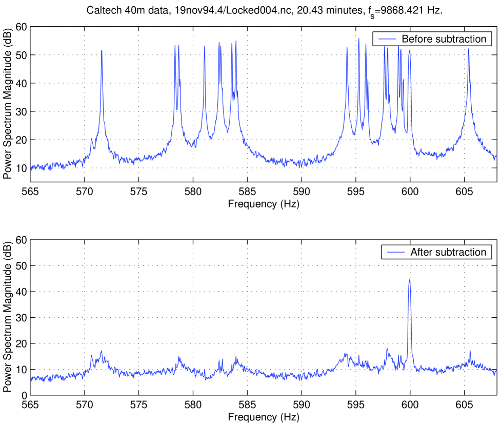
Here we describe the design of a Kalman filter that determines the time-dependent vibrational state of a detector’s suspension “violin” modes from time dependent observations of the detector output. From the estimated state we can predict that component of the detector output due to suspension excitations, thermal or otherwise. The wire state can be examined for evidence of suspension disturbances that might, in the absence of such a diagnostic, be mistaken for gravitational wave signals. Additionally, from the wire state we can subtractively remove the contribution from suspension disturbances, thermal or otherwise, from the detector output, leaving a residual free from this instrumental artifact. We demonstrate the filter’s effectiveness both through numerical simulations and application to real data taken on the LIGO 40 M prototype detector.

I Introduction

Within the next several years five kilometer-scale interferometric gravitational wave detectors (GEO [1], LIGO [2] and VIRGO [3]) will begin searching for astronomical sources of gravitational waves, something the smaller TAMA [4] prototype detector has already begun. The fundamental limitation on the sensitivity of these terrestrial detectors is seismic noise at low frequencies, thermal excitations of the mirror substrates and their suspensions at intermediate frequencies, and laser shot noise at higher frequencies. Here we focus on that part of the suspension noise associated with the violin modes of the suspension wires.

Gravitational waves interact with interferometric detectors by changing the separation, and thus the round-trip light travel time, between the mirrors in the detector arms. In order to be sensitive to passing gravitational radiation, the mirrors in terrestrial interferometeric detectors are suspended as pendula in order that they be approximately inertially free above the pendulumn frequency. Nevertheless, thermal and other excitations of the suspension wires move the mirrors and lead to (narrow-band) data stream artifacts, located at the violin-mode resonance frequencies of the suspension wires. These narrow-band features, which stand some 40–60 dB above the shot noise background in the LIGO I detector, are signals themselves that, unless properly treated, can confound efforts to detect actual gravitational wave signals.

In the waveband of the detectors now under development the transfer function, which determines how the detector output at a particular frequency is related to incident radiation at that frequency, is constant. The time evolution of the signal arising from any incident gravitational waves is thus determined solely by the waves themselves. The time evolution of the signal arising from suspension violin mode excitations, on the other hand, is strongly influenced by the the dynamics of the modes. We make use of that distinction to design a Kalman filter [5] that can, in real-time, detect violin mode excitations — thermal or otherwise — as distinct from actual gravitational wave signals. The measured excitation can be used to subtractively remove the modes from the detector output, significantly reducing the rms detector noise and simplifying the down-stream analysis. Additionally, these measured excitations can be used to diagnose the instrument’s behavior.

Other techniques have been described for the identification and removal of resonant line features in gravitational wave detector data. In particular, Sintes and Schutz [6, 7] have discussed methods suitable for addressing nearly periodic artifacts that appear in a range of harmonics and whose phases, in each harmonic, are linearly related. These methods are not suitable for isolating the violin modes, however: though a full spectrum of violin mode harmonics do appear in the detector output, these modes are all independent and independently excited. Allen and Ottewill [8] have applied the multi-taper spectral method of Lees and Park[9] to estimate the contributions of these resonant features to the power spectrum. This non-parametric method does not and cannot provide a time-domain estimate of the mode state or its instantaneous contribution to the detector output and so cannot be used for conditioning the data prior to analysis.

In section II we summarize the theory of Kalman Filtering, laying the ground for its application to identifying gravitational wave detector suspension violin modes. The construction of the Kalman filter for a particular problem requires a dynamical model for the underlying physical process giving rise to the signal. We discuss our model and how it comes to be represented as a set of state-space difference equations on the physical observables. In section V we investigate the performance of the filter using both simulated data sets, whose “signal” and “noise” content is known exactly, and experimental data taken at the LIGO 40 M prototype detector during November 1994. We summarize our conclusions in section VI.

II The Kalman Filter

A Introduction

A Kalman filter is a mechanism for predicting the multi-dimensional state of a dynamical system from a multi-dimensional observable. The observable is assumed to be linearly related to the system’s state, which is assumed to evolve linearly with time. The observable is assumed to be contaminated by an additive Gaussian measurement noise of known co-variance. The dynamical system described by the state may be driven by a known input in addition to Gaussian process noise of known co-variance.

For example, the system may be a pendulum, the state may be the pendulum bob’s instantaneous position and momentum, and the observable may be the bob’s position. The process noise is the thermal fluctuation in the wire and the measurement noise in this case may be the photon shot noise background.

When the process and measurement noise are Normal (i.e., Gaussian) the Kalman filter gives the optimal estimate of the system’s state, in the least-squares sense. When the noise is more complex than Gaussian the Kalman filter gives the best estimate of the state assuming that only the second order statistical characterization of the noise is known. Alternatively, when the evolution equations are not linear or the observables are not related linearly to the state, then the Kalman filter has a natural generalization that makes it the optimal means of predicting the state from the observables in a least-squares sense [11].

The derivation of the Kalman Filter equations is straightforward and instructive. In the particular application dealt with in this paper we assume that there is no driving force (aside from the process noise) and that the system state and observables are needed only at discrete times; correspondingly, we limit our derivation to that case. Denote the state of the system at sample time $k$ by $\mathchoice{{\hbox{\boldmath$\displaystyle\psi$}}}{{\hbox{\boldmath$\textstyle\psi$}}}{{\hbox{\boldmath$\scriptstyle\psi$}}}{{\hbox{\boldmath$\scriptscriptstyle\psi$}}}[k]$ and the observable at sample time $k$ by $\mathchoice{{\hbox{\boldmath$\displaystyle z$}}}{{\hbox{\boldmath$\textstyle z$}}}{{\hbox{\boldmath$\scriptstyle z$}}}{{\hbox{\boldmath$\scriptscriptstyle z$}}}[k]$:

$$\mathchoice{{\hbox{\boldmath$\displaystyle\psi$}}}{{\hbox{\boldmath$\textstyle\psi$}}}{{\hbox{\boldmath$\scriptstyle\psi$}}}{{\hbox{\boldmath$\scriptscriptstyle\psi$}}}[k] := \left(\begin{array}[]{l}\text{The state vector of the dynamical}\\ \text{system at sample $k$; a $M\times 1$ vector}\end{array}\right)$$ (4)

$$\mathchoice{{\hbox{\boldmath$\displaystyle z$}}}{{\hbox{\boldmath$\textstyle z$}}}{{\hbox{\boldmath$\scriptstyle z$}}}{{\hbox{\boldmath$\scriptscriptstyle z$}}}[k] := \left(\begin{array}[]{l}\text{The system observable at}\\ \text{sample $k$; a $N\times 1$ vector}\end{array}\right).$$ (7)

The state $\textstyle\psi$ evolves from one sample to the next according to the linear equation

$$\mathchoice{{\hbox{\boldmath$\displaystyle\psi$}}}{{\hbox{\boldmath$\textstyle\psi$}}}{{\hbox{\boldmath$\scriptstyle\psi$}}}{{\hbox{\boldmath$\scriptscriptstyle\psi$}}}[k+1]=\mathchoice{{\hbox{\boldmath$\displaystyle A$}}}{{\hbox{\boldmath$\textstyle A$}}}{{\hbox{\boldmath$\scriptstyle A$}}}{{\hbox{\boldmath$\scriptscriptstyle A$}}}\cdot\mathchoice{{\hbox{\boldmath$\displaystyle\psi$}}}{{\hbox{\boldmath$\textstyle\psi$}}}{{\hbox{\boldmath$\scriptstyle\psi$}}}{{\hbox{\boldmath$\scriptscriptstyle\psi$}}}[k]+\mathchoice{{\hbox{\boldmath$\displaystyle w$}}}{{\hbox{\boldmath$\textstyle w$}}}{{\hbox{\boldmath$\scriptstyle w$}}}{{\hbox{\boldmath$\scriptscriptstyle w$}}}[k],$$ (8)

where $\textstyle A$ is a linear operator and $\mathchoice{{\hbox{\boldmath$\displaystyle w$}}}{{\hbox{\boldmath$\textstyle w$}}}{{\hbox{\boldmath$\scriptstyle w$}}}{{\hbox{\boldmath$\scriptscriptstyle w$}}}[k]$ is an instance of process noise:

$$A := \left(\begin{array}[]{l}\text{Linear transformation that}\\ \text{takes $\mathchoice{{\hbox{\boldmath$\displaystyle\psi$}}}{{\hbox{\boldmath$\textstyle\psi$}}}{{\hbox{\boldmath$\scriptstyle\psi$}}}{{\hbox{\boldmath$\scriptscriptstyle\psi$}}}[k]$ to $\mathchoice{{\hbox{\boldmath$\displaystyle\psi$}}}{{\hbox{\boldmath$\textstyle\psi$}}}{{\hbox{\boldmath$\scriptstyle\psi$}}}{{\hbox{\boldmath$\scriptscriptstyle\psi$}}}[k+1]$;}\\ \text{a $M\times M$ matrix}\end{array}\right)$$ (12)

$$w := \left(\begin{array}[]{l}\text{Process noise: a $M$-dimensional}\\ \text{Normally distributed random}\\ \text{variable; a $M\times 1$ vector.}\end{array}\right)$$ (16)

The process noise is assumed to be zero mean and white. It is then fully characterized by its co-variance matrix $\textstyle W$:

$$\mathchoice{{\hbox{\boldmath$\displaystyle W$}}}{{\hbox{\boldmath$\textstyle W$}}}{{\hbox{\boldmath$\scriptstyle W$}}}{{\hbox{\boldmath$\scriptscriptstyle W$}}}:=E[{\mathchoice{{\hbox{\boldmath$\displaystyle w$}}}{{\hbox{\boldmath$\textstyle w$}}}{{\hbox{\boldmath$\scriptstyle w$}}}{{\hbox{\boldmath$\scriptscriptstyle w$}}}\cdot\mathchoice{{\hbox{\boldmath$\displaystyle w$}}}{{\hbox{\boldmath$\textstyle w$}}}{{\hbox{\boldmath$\scriptstyle w$}}}{{\hbox{\boldmath$\scriptscriptstyle w$}}}^{T}}],$$ (17)

where $E[\cdot]$ represents an ensemble average across instances of its argument. The process noise co-variance is a symmetric $M\times M$ constant matrix.

The observable $\textstyle z$ at sample $k$ is related to the system state by the linear equation

$$\mathchoice{{\hbox{\boldmath$\displaystyle z$}}}{{\hbox{\boldmath$\textstyle z$}}}{{\hbox{\boldmath$\scriptstyle z$}}}{{\hbox{\boldmath$\scriptscriptstyle z$}}}[k]=\mathchoice{{\hbox{\boldmath$\displaystyle C$}}}{{\hbox{\boldmath$\textstyle C$}}}{{\hbox{\boldmath$\scriptstyle C$}}}{{\hbox{\boldmath$\scriptscriptstyle C$}}}\cdot\mathchoice{{\hbox{\boldmath$\displaystyle\psi$}}}{{\hbox{\boldmath$\textstyle\psi$}}}{{\hbox{\boldmath$\scriptstyle\psi$}}}{{\hbox{\boldmath$\scriptscriptstyle\psi$}}}[k]+\mathchoice{{\hbox{\boldmath$\displaystyle v$}}}{{\hbox{\boldmath$\textstyle v$}}}{{\hbox{\boldmath$\scriptstyle v$}}}{{\hbox{\boldmath$\scriptscriptstyle v$}}}[k],$$ (18)

where $\textstyle C$ is a linear operator and $\mathchoice{{\hbox{\boldmath$\displaystyle v$}}}{{\hbox{\boldmath$\textstyle v$}}}{{\hbox{\boldmath$\scriptstyle v$}}}{{\hbox{\boldmath$\scriptscriptstyle v$}}}[k]$ is an instance of measurement noise:

$$C := \left(\begin{array}[]{l}\text{The linear transformation}\\ \text{that relates the state $\mathchoice{{\hbox{\boldmath$\displaystyle\psi$}}}{{\hbox{\boldmath$\textstyle\psi$}}}{{\hbox{\boldmath$\scriptstyle\psi$}}}{{\hbox{\boldmath$\scriptscriptstyle\psi$}}}[k]$}\\ \text{to the observable $\mathchoice{{\hbox{\boldmath$\displaystyle z$}}}{{\hbox{\boldmath$\textstyle z$}}}{{\hbox{\boldmath$\scriptstyle z$}}}{{\hbox{\boldmath$\scriptscriptstyle z$}}}[k]$; an}\\ \text{$N\times M$ matrix}\end{array}\right)$$ (23)

$$\mathchoice{{\hbox{\boldmath$\displaystyle v$}}}{{\hbox{\boldmath$\textstyle v$}}}{{\hbox{\boldmath$\scriptstyle v$}}}{{\hbox{\boldmath$\scriptscriptstyle v$}}}[k] := \left(\begin{array}[]{l}\text{Measurement noise: a $N$-dimensional}\\ \text{Normally distributed random variable;}\\ \text{a $N\times 1$ vector}\end{array}\right).$$ (27)

The measurement noise is assumed to be zero mean, white, and have co-variance $\textstyle V$:

$$\mathchoice{{\hbox{\boldmath$\displaystyle V$}}}{{\hbox{\boldmath$\textstyle V$}}}{{\hbox{\boldmath$\scriptstyle V$}}}{{\hbox{\boldmath$\scriptscriptstyle V$}}}:=E[{\mathchoice{{\hbox{\boldmath$\displaystyle v$}}}{{\hbox{\boldmath$\textstyle v$}}}{{\hbox{\boldmath$\scriptstyle v$}}}{{\hbox{\boldmath$\scriptscriptstyle v$}}}\cdot\mathchoice{{\hbox{\boldmath$\displaystyle v$}}}{{\hbox{\boldmath$\textstyle v$}}}{{\hbox{\boldmath$\scriptstyle v$}}}{{\hbox{\boldmath$\scriptscriptstyle v$}}}^{T}}],$$ (28)

where $E[\cdot]$ represents an ensemble average across instances of $\mathchoice{{\hbox{\boldmath$\displaystyle v$}}}{{\hbox{\boldmath$\textstyle v$}}}{{\hbox{\boldmath$\scriptstyle v$}}}{{\hbox{\boldmath$\scriptscriptstyle v$}}}[k]$ of the measurement noise. The measurement noise co-variance is a symmetric $N\times N$ matrix.

Finally, we assume that the measurement noise and process noise are independent:

$$E[\mathchoice{{\hbox{\boldmath$\displaystyle v$}}}{{\hbox{\boldmath$\textstyle v$}}}{{\hbox{\boldmath$\scriptstyle v$}}}{{\hbox{\boldmath$\scriptscriptstyle v$}}}\cdot\mathchoice{{\hbox{\boldmath$\displaystyle w$}}}{{\hbox{\boldmath$\textstyle w$}}}{{\hbox{\boldmath$\scriptstyle w$}}}{{\hbox{\boldmath$\scriptscriptstyle w$}}}^{T}]=0.$$ (29)

B Predicting the state from observations

Suppose that we have an estimate $\widehat{\mathchoice{{\hbox{\boldmath$\displaystyle\psi$}}}{{\hbox{\boldmath$\textstyle\psi$}}}{{\hbox{\boldmath$\scriptstyle\psi$}}}{{\hbox{\boldmath$\scriptscriptstyle\psi$}}}}[k-1]$ of the process state at sample $k-1$. Denote the error in this estimate by $\widehat{\mathchoice{{\hbox{\boldmath$\displaystyle e$}}}{{\hbox{\boldmath$\textstyle e$}}}{{\hbox{\boldmath$\scriptstyle e$}}}{{\hbox{\boldmath$\scriptscriptstyle e$}}}}[k-1]$:

$$\widehat{\mathchoice{{\hbox{\boldmath$\displaystyle e$}}}{{\hbox{\boldmath$\textstyle e$}}}{{\hbox{\boldmath$\scriptstyle e$}}}{{\hbox{\boldmath$\scriptscriptstyle e$}}}}[k-1]:=\mathchoice{{\hbox{\boldmath$\displaystyle\psi$}}}{{\hbox{\boldmath$\textstyle\psi$}}}{{\hbox{\boldmath$\scriptstyle\psi$}}}{{\hbox{\boldmath$\scriptscriptstyle\psi$}}}[k-1]-\widehat{\mathchoice{{\hbox{\boldmath$\displaystyle\psi$}}}{{\hbox{\boldmath$\textstyle\psi$}}}{{\hbox{\boldmath$\scriptstyle\psi$}}}{{\hbox{\boldmath$\scriptscriptstyle\psi$}}}}[k-1].$$ (30)

This error is a random variable whose second moments we denote $\mathchoice{{\hbox{\boldmath$\displaystyle P$}}}{{\hbox{\boldmath$\textstyle P$}}}{{\hbox{\boldmath$\scriptstyle P$}}}{{\hbox{\boldmath$\scriptscriptstyle P$}}}[k-1]$:

$$\widehat{\mathchoice{{\hbox{\boldmath$\displaystyle P$}}}{{\hbox{\boldmath$\textstyle P$}}}{{\hbox{\boldmath$\scriptstyle P$}}}{{\hbox{\boldmath$\scriptscriptstyle P$}}}}[k-1]:=E[\widehat{\mathchoice{{\hbox{\boldmath$\displaystyle e$}}}{{\hbox{\boldmath$\textstyle e$}}}{{\hbox{\boldmath$\scriptstyle e$}}}{{\hbox{\boldmath$\scriptscriptstyle e$}}}}[k-1]\cdot\widehat{\mathchoice{{\hbox{\boldmath$\displaystyle e$}}}{{\hbox{\boldmath$\textstyle e$}}}{{\hbox{\boldmath$\scriptstyle e$}}}{{\hbox{\boldmath$\scriptscriptstyle e$}}}}^{T}[k-1]].$$ (31)

From the estimated state at sample $k-1$, we can form an a priori estimate of the state at sample $k$ using the state transition operator $\textstyle A$:

$$\widetilde{\mathchoice{{\hbox{\boldmath$\displaystyle\psi$}}}{{\hbox{\boldmath$\textstyle\psi$}}}{{\hbox{\boldmath$\scriptstyle\psi$}}}{{\hbox{\boldmath$\scriptscriptstyle\psi$}}}}[k]:=\mathchoice{{\hbox{\boldmath$\displaystyle A$}}}{{\hbox{\boldmath$\textstyle A$}}}{{\hbox{\boldmath$\scriptstyle A$}}}{{\hbox{\boldmath$\scriptscriptstyle A$}}}\cdot\widehat{\mathchoice{{\hbox{\boldmath$\displaystyle\psi$}}}{{\hbox{\boldmath$\textstyle\psi$}}}{{\hbox{\boldmath$\scriptstyle\psi$}}}{{\hbox{\boldmath$\scriptscriptstyle\psi$}}}}[k-1].$$ (32)

Associated with $\widetilde{\mathchoice{{\hbox{\boldmath$\displaystyle\psi$}}}{{\hbox{\boldmath$\textstyle\psi$}}}{{\hbox{\boldmath$\scriptstyle\psi$}}}{{\hbox{\boldmath$\scriptscriptstyle\psi$}}}}[k]$ is an error $\widetilde{\mathchoice{{\hbox{\boldmath$\displaystyle e$}}}{{\hbox{\boldmath$\textstyle e$}}}{{\hbox{\boldmath$\scriptstyle e$}}}{{\hbox{\boldmath$\scriptscriptstyle e$}}}}[k]$ whose second moments we denote $\widetilde{\mathchoice{{\hbox{\boldmath$\displaystyle P$}}}{{\hbox{\boldmath$\textstyle P$}}}{{\hbox{\boldmath$\scriptstyle P$}}}{{\hbox{\boldmath$\scriptscriptstyle P$}}}}[k]$:

$$\widetilde{\mathchoice{{\hbox{\boldmath$\displaystyle e$}}}{{\hbox{\boldmath$\textstyle e$}}}{{\hbox{\boldmath$\scriptstyle e$}}}{{\hbox{\boldmath$\scriptscriptstyle e$}}}}[k] := \mathchoice{{\hbox{\boldmath$\displaystyle\psi$}}}{{\hbox{\boldmath$\textstyle\psi$}}}{{\hbox{\boldmath$\scriptstyle\psi$}}}{{\hbox{\boldmath$\scriptscriptstyle\psi$}}}[k]-\widetilde{\mathchoice{{\hbox{\boldmath$\displaystyle\psi$}}}{{\hbox{\boldmath$\textstyle\psi$}}}{{\hbox{\boldmath$\scriptstyle\psi$}}}{{\hbox{\boldmath$\scriptscriptstyle\psi$}}}}[k].$$ (34)

$$\widetilde{\mathchoice{{\hbox{\boldmath$\displaystyle P$}}}{{\hbox{\boldmath$\textstyle P$}}}{{\hbox{\boldmath$\scriptstyle P$}}}{{\hbox{\boldmath$\scriptscriptstyle P$}}}}[k] := E[\widetilde{\mathchoice{{\hbox{\boldmath$\displaystyle e$}}}{{\hbox{\boldmath$\textstyle e$}}}{{\hbox{\boldmath$\scriptstyle e$}}}{{\hbox{\boldmath$\scriptscriptstyle e$}}}}[k]\cdot\widetilde{\mathchoice{{\hbox{\boldmath$\displaystyle e$}}}{{\hbox{\boldmath$\textstyle e$}}}{{\hbox{\boldmath$\scriptstyle e$}}}{{\hbox{\boldmath$\scriptscriptstyle e$}}}}^{T}[k]]$$ (35)

$$= \mathchoice{{\hbox{\boldmath$\displaystyle A$}}}{{\hbox{\boldmath$\textstyle A$}}}{{\hbox{\boldmath$\scriptstyle A$}}}{{\hbox{\boldmath$\scriptscriptstyle A$}}}\cdot\widehat{P}[k-1]\cdot\mathchoice{{\hbox{\boldmath$\displaystyle A$}}}{{\hbox{\boldmath$\textstyle A$}}}{{\hbox{\boldmath$\scriptstyle A$}}}{{\hbox{\boldmath$\scriptscriptstyle A$}}}^{T}+\mathchoice{{\hbox{\boldmath$\displaystyle W$}}}{{\hbox{\boldmath$\textstyle W$}}}{{\hbox{\boldmath$\scriptstyle W$}}}{{\hbox{\boldmath$\scriptscriptstyle W$}}}.$$ (36)

The final equality follows from equations 34, 8 and 17.

From $\widetilde{\psi}[k]$, we can make a prediction $\widetilde{\mathchoice{{\hbox{\boldmath$\displaystyle z$}}}{{\hbox{\boldmath$\textstyle z$}}}{{\hbox{\boldmath$\scriptstyle z$}}}{{\hbox{\boldmath$\scriptscriptstyle z$}}}}$ of the observable $\mathchoice{{\hbox{\boldmath$\displaystyle z$}}}{{\hbox{\boldmath$\textstyle z$}}}{{\hbox{\boldmath$\scriptstyle z$}}}{{\hbox{\boldmath$\scriptscriptstyle z$}}}[k]$:

$$\widetilde{\mathchoice{{\hbox{\boldmath$\displaystyle z$}}}{{\hbox{\boldmath$\textstyle z$}}}{{\hbox{\boldmath$\scriptstyle z$}}}{{\hbox{\boldmath$\scriptscriptstyle z$}}}}[k]=\mathchoice{{\hbox{\boldmath$\displaystyle C$}}}{{\hbox{\boldmath$\textstyle C$}}}{{\hbox{\boldmath$\scriptstyle C$}}}{{\hbox{\boldmath$\scriptscriptstyle C$}}}\cdot\widetilde{\mathchoice{{\hbox{\boldmath$\displaystyle\psi$}}}{{\hbox{\boldmath$\textstyle\psi$}}}{{\hbox{\boldmath$\scriptstyle\psi$}}}{{\hbox{\boldmath$\scriptscriptstyle\psi$}}}}[k].$$ (37)

Now compare the estimate $\widetilde{\mathchoice{{\hbox{\boldmath$\displaystyle z$}}}{{\hbox{\boldmath$\textstyle z$}}}{{\hbox{\boldmath$\scriptstyle z$}}}{{\hbox{\boldmath$\scriptscriptstyle z$}}}}[k]$ to the actual measurement $\mathchoice{{\hbox{\boldmath$\displaystyle z$}}}{{\hbox{\boldmath$\textstyle z$}}}{{\hbox{\boldmath$\scriptstyle z$}}}{{\hbox{\boldmath$\scriptscriptstyle z$}}}[k]$. These will in general be different. The Kalman Filter uses the difference between the the actual and estimated measurement to generate a corrected estimate $\widehat{\mathchoice{{\hbox{\boldmath$\displaystyle\psi$}}}{{\hbox{\boldmath$\textstyle\psi$}}}{{\hbox{\boldmath$\scriptstyle\psi$}}}{{\hbox{\boldmath$\scriptscriptstyle\psi$}}}}$ of the state:

$$\widehat{\mathchoice{{\hbox{\boldmath$\displaystyle\psi$}}}{{\hbox{\boldmath$\textstyle\psi$}}}{{\hbox{\boldmath$\scriptstyle\psi$}}}{{\hbox{\boldmath$\scriptscriptstyle\psi$}}}}[k]=\widetilde{\mathchoice{{\hbox{\boldmath$\displaystyle\psi$}}}{{\hbox{\boldmath$\textstyle\psi$}}}{{\hbox{\boldmath$\scriptstyle\psi$}}}{{\hbox{\boldmath$\scriptscriptstyle\psi$}}}}[k]+\mathchoice{{\hbox{\boldmath$\displaystyle K$}}}{{\hbox{\boldmath$\textstyle K$}}}{{\hbox{\boldmath$\scriptstyle K$}}}{{\hbox{\boldmath$\scriptscriptstyle K$}}}[k]\cdot\left(\mathchoice{{\hbox{\boldmath$\displaystyle z$}}}{{\hbox{\boldmath$\textstyle z$}}}{{\hbox{\boldmath$\scriptstyle z$}}}{{\hbox{\boldmath$\scriptscriptstyle z$}}}[k]-\widetilde{\mathchoice{{\hbox{\boldmath$\displaystyle z$}}}{{\hbox{\boldmath$\textstyle z$}}}{{\hbox{\boldmath$\scriptstyle z$}}}{{\hbox{\boldmath$\scriptscriptstyle z$}}}}[k]\right).$$ (38)

The linear operator $\mathchoice{{\hbox{\boldmath$\displaystyle K$}}}{{\hbox{\boldmath$\textstyle K$}}}{{\hbox{\boldmath$\scriptstyle K$}}}{{\hbox{\boldmath$\scriptscriptstyle K$}}}[k]$ is the Kalman gain, which we calculate in section II C. The refined state estimate $\widehat{\mathchoice{{\hbox{\boldmath$\displaystyle\psi$}}}{{\hbox{\boldmath$\textstyle\psi$}}}{{\hbox{\boldmath$\scriptstyle\psi$}}}{{\hbox{\boldmath$\scriptscriptstyle\psi$}}}}[k]$ has an associated error $\widehat{\mathchoice{{\hbox{\boldmath$\displaystyle e$}}}{{\hbox{\boldmath$\textstyle e$}}}{{\hbox{\boldmath$\scriptstyle e$}}}{{\hbox{\boldmath$\scriptscriptstyle e$}}}}[k]$ (cf. eq. 30) and covariance $\widehat{\mathchoice{{\hbox{\boldmath$\displaystyle P$}}}{{\hbox{\boldmath$\textstyle P$}}}{{\hbox{\boldmath$\scriptstyle P$}}}{{\hbox{\boldmath$\scriptscriptstyle P$}}}}[k]$ (cf. eq. 31):

$$\widehat{\mathchoice{{\hbox{\boldmath$\displaystyle P$}}}{{\hbox{\boldmath$\textstyle P$}}}{{\hbox{\boldmath$\scriptstyle P$}}}{{\hbox{\boldmath$\scriptscriptstyle P$}}}}=\left(\mathchoice{{\hbox{\boldmath$\displaystyle I$}}}{{\hbox{\boldmath$\textstyle I$}}}{{\hbox{\boldmath$\scriptstyle I$}}}{{\hbox{\boldmath$\scriptscriptstyle I$}}}-\mathchoice{{\hbox{\boldmath$\displaystyle K$}}}{{\hbox{\boldmath$\textstyle K$}}}{{\hbox{\boldmath$\scriptstyle K$}}}{{\hbox{\boldmath$\scriptscriptstyle K$}}}\cdot\mathchoice{{\hbox{\boldmath$\displaystyle C$}}}{{\hbox{\boldmath$\textstyle C$}}}{{\hbox{\boldmath$\scriptstyle C$}}}{{\hbox{\boldmath$\scriptscriptstyle C$}}}\right)\cdot\widetilde{\mathchoice{{\hbox{\boldmath$\displaystyle P$}}}{{\hbox{\boldmath$\textstyle P$}}}{{\hbox{\boldmath$\scriptstyle P$}}}{{\hbox{\boldmath$\scriptscriptstyle P$}}}}\cdot\left(\mathchoice{{\hbox{\boldmath$\displaystyle I$}}}{{\hbox{\boldmath$\textstyle I$}}}{{\hbox{\boldmath$\scriptstyle I$}}}{{\hbox{\boldmath$\scriptscriptstyle I$}}}-\mathchoice{{\hbox{\boldmath$\displaystyle K$}}}{{\hbox{\boldmath$\textstyle K$}}}{{\hbox{\boldmath$\scriptstyle K$}}}{{\hbox{\boldmath$\scriptscriptstyle K$}}}\cdot\mathchoice{{\hbox{\boldmath$\displaystyle C$}}}{{\hbox{\boldmath$\textstyle C$}}}{{\hbox{\boldmath$\scriptstyle C$}}}{{\hbox{\boldmath$\scriptscriptstyle C$}}}\right)^{T},$$ (39)

where $\textstyle I$ is the identity matrix and we have used 30, 34 and 38 to represent $\widehat{\mathchoice{{\hbox{\boldmath$\displaystyle P$}}}{{\hbox{\boldmath$\textstyle P$}}}{{\hbox{\boldmath$\scriptstyle P$}}}{{\hbox{\boldmath$\scriptscriptstyle P$}}}}$ in terms of the unknown $\textstyle K$ and the known $\textstyle C$ and $\widetilde{\mathchoice{{\hbox{\boldmath$\displaystyle P$}}}{{\hbox{\boldmath$\textstyle P$}}}{{\hbox{\boldmath$\scriptstyle P$}}}{{\hbox{\boldmath$\scriptscriptstyle P$}}}}$, all at sample $k$.

C Calculating the Kalman Gain

Our object is to find the Kalman gain $\textstyle K$ that minimizes an appropriate measure of the error $\widehat{\mathchoice{{\hbox{\boldmath$\displaystyle P$}}}{{\hbox{\boldmath$\textstyle P$}}}{{\hbox{\boldmath$\scriptstyle P$}}}{{\hbox{\boldmath$\scriptscriptstyle P$}}}}$ in the state estimate $\widehat{\psi}$ at each sample $k$.

Recall that $\widehat{\mathchoice{{\hbox{\boldmath$\displaystyle P$}}}{{\hbox{\boldmath$\textstyle P$}}}{{\hbox{\boldmath$\scriptstyle P$}}}{{\hbox{\boldmath$\scriptscriptstyle P$}}}}$ is a co-variance matrix of the error $\widehat{\mathchoice{{\hbox{\boldmath$\displaystyle e$}}}{{\hbox{\boldmath$\textstyle e$}}}{{\hbox{\boldmath$\scriptstyle e$}}}{{\hbox{\boldmath$\scriptscriptstyle e$}}}}$; consequently, its eigenvectors describe linear combination of the state vector elements whose errors are uncorrelated. Correspondingly, the sum of the eigenvalues — the trace of $\widehat{\mathchoice{{\hbox{\boldmath$\displaystyle P$}}}{{\hbox{\boldmath$\textstyle P$}}}{{\hbox{\boldmath$\scriptstyle P$}}}{{\hbox{\boldmath$\scriptscriptstyle P$}}}}$ — measures the variance of the total error in the state estimate. Adopting $\text{tr}\,\widehat{\mathchoice{{\hbox{\boldmath$\displaystyle P$}}}{{\hbox{\boldmath$\textstyle P$}}}{{\hbox{\boldmath$\scriptstyle P$}}}{{\hbox{\boldmath$\scriptscriptstyle P$}}}}$ as a measure of the error in the state estimate, we choose the Kalman gain $\textstyle K$ to minimize $\text{tr}\,\widehat{\mathchoice{{\hbox{\boldmath$\displaystyle P$}}}{{\hbox{\boldmath$\textstyle P$}}}{{\hbox{\boldmath$\scriptstyle P$}}}{{\hbox{\boldmath$\scriptscriptstyle P$}}}}$:

$$\mathchoice{{\hbox{\boldmath$\displaystyle K$}}}{{\hbox{\boldmath$\textstyle K$}}}{{\hbox{\boldmath$\scriptstyle K$}}}{{\hbox{\boldmath$\scriptscriptstyle K$}}}[k] = \widetilde{\mathchoice{{\hbox{\boldmath$\displaystyle P$}}}{{\hbox{\boldmath$\textstyle P$}}}{{\hbox{\boldmath$\scriptstyle P$}}}{{\hbox{\boldmath$\scriptscriptstyle P$}}}}[k]\cdot\mathchoice{{\hbox{\boldmath$\displaystyle C$}}}{{\hbox{\boldmath$\textstyle C$}}}{{\hbox{\boldmath$\scriptstyle C$}}}{{\hbox{\boldmath$\scriptscriptstyle C$}}}^{T}/\left(\mathchoice{{\hbox{\boldmath$\displaystyle V$}}}{{\hbox{\boldmath$\textstyle V$}}}{{\hbox{\boldmath$\scriptstyle V$}}}{{\hbox{\boldmath$\scriptscriptstyle V$}}}+\mathchoice{{\hbox{\boldmath$\displaystyle C$}}}{{\hbox{\boldmath$\textstyle C$}}}{{\hbox{\boldmath$\scriptstyle C$}}}{{\hbox{\boldmath$\scriptscriptstyle C$}}}\cdot\widetilde{\mathchoice{{\hbox{\boldmath$\displaystyle P$}}}{{\hbox{\boldmath$\textstyle P$}}}{{\hbox{\boldmath$\scriptstyle P$}}}{{\hbox{\boldmath$\scriptscriptstyle P$}}}}[k]\cdot\mathchoice{{\hbox{\boldmath$\displaystyle C$}}}{{\hbox{\boldmath$\textstyle C$}}}{{\hbox{\boldmath$\scriptstyle C$}}}{{\hbox{\boldmath$\scriptscriptstyle C$}}}^{T}\right),$$ (40)

where we have adopted the notation

$$\mathchoice{{\hbox{\boldmath$\displaystyle Q$}}}{{\hbox{\boldmath$\textstyle Q$}}}{{\hbox{\boldmath$\scriptstyle Q$}}}{{\hbox{\boldmath$\scriptscriptstyle Q$}}}=\mathchoice{{\hbox{\boldmath$\displaystyle S$}}}{{\hbox{\boldmath$\textstyle S$}}}{{\hbox{\boldmath$\scriptstyle S$}}}{{\hbox{\boldmath$\scriptscriptstyle S$}}}/\mathchoice{{\hbox{\boldmath$\displaystyle R$}}}{{\hbox{\boldmath$\textstyle R$}}}{{\hbox{\boldmath$\scriptstyle R$}}}{{\hbox{\boldmath$\scriptscriptstyle R$}}}$$ (42)

to denote $\textstyle Q$ as a solution to the linear equation

$$\mathchoice{{\hbox{\boldmath$\displaystyle S$}}}{{\hbox{\boldmath$\textstyle S$}}}{{\hbox{\boldmath$\scriptstyle S$}}}{{\hbox{\boldmath$\scriptscriptstyle S$}}}=\mathchoice{{\hbox{\boldmath$\displaystyle Q$}}}{{\hbox{\boldmath$\textstyle Q$}}}{{\hbox{\boldmath$\scriptstyle Q$}}}{{\hbox{\boldmath$\scriptscriptstyle Q$}}}\cdot\mathchoice{{\hbox{\boldmath$\displaystyle R$}}}{{\hbox{\boldmath$\textstyle R$}}}{{\hbox{\boldmath$\scriptstyle R$}}}{{\hbox{\boldmath$\scriptscriptstyle R$}}}$$ (43)

for known $\textstyle R$, $\textstyle S$. Correspondingly, equation 39 for $\widehat{\mathchoice{{\hbox{\boldmath$\displaystyle P$}}}{{\hbox{\boldmath$\textstyle P$}}}{{\hbox{\boldmath$\scriptstyle P$}}}{{\hbox{\boldmath$\scriptscriptstyle P$}}}}$ can be simplified:

$$\widehat{\mathchoice{{\hbox{\boldmath$\displaystyle P$}}}{{\hbox{\boldmath$\textstyle P$}}}{{\hbox{\boldmath$\scriptstyle P$}}}{{\hbox{\boldmath$\scriptscriptstyle P$}}}} = \left(\mathchoice{{\hbox{\boldmath$\displaystyle I$}}}{{\hbox{\boldmath$\textstyle I$}}}{{\hbox{\boldmath$\scriptstyle I$}}}{{\hbox{\boldmath$\scriptscriptstyle I$}}}-\mathchoice{{\hbox{\boldmath$\displaystyle K$}}}{{\hbox{\boldmath$\textstyle K$}}}{{\hbox{\boldmath$\scriptstyle K$}}}{{\hbox{\boldmath$\scriptscriptstyle K$}}}\cdot\mathchoice{{\hbox{\boldmath$\displaystyle C$}}}{{\hbox{\boldmath$\textstyle C$}}}{{\hbox{\boldmath$\scriptstyle C$}}}{{\hbox{\boldmath$\scriptscriptstyle C$}}}\right)\cdot\widetilde{\mathchoice{{\hbox{\boldmath$\displaystyle P$}}}{{\hbox{\boldmath$\textstyle P$}}}{{\hbox{\boldmath$\scriptstyle P$}}}{{\hbox{\boldmath$\scriptscriptstyle P$}}}}\cdot\left(\mathchoice{{\hbox{\boldmath$\displaystyle I$}}}{{\hbox{\boldmath$\textstyle I$}}}{{\hbox{\boldmath$\scriptstyle I$}}}{{\hbox{\boldmath$\scriptscriptstyle I$}}}-\mathchoice{{\hbox{\boldmath$\displaystyle K$}}}{{\hbox{\boldmath$\textstyle K$}}}{{\hbox{\boldmath$\scriptstyle K$}}}{{\hbox{\boldmath$\scriptscriptstyle K$}}}\cdot\mathchoice{{\hbox{\boldmath$\displaystyle C$}}}{{\hbox{\boldmath$\textstyle C$}}}{{\hbox{\boldmath$\scriptstyle C$}}}{{\hbox{\boldmath$\scriptscriptstyle C$}}}\right)^{T}$$ (44)

$$= \left(\mathchoice{{\hbox{\boldmath$\displaystyle I$}}}{{\hbox{\boldmath$\textstyle I$}}}{{\hbox{\boldmath$\scriptstyle I$}}}{{\hbox{\boldmath$\scriptscriptstyle I$}}}-\mathchoice{{\hbox{\boldmath$\displaystyle K$}}}{{\hbox{\boldmath$\textstyle K$}}}{{\hbox{\boldmath$\scriptstyle K$}}}{{\hbox{\boldmath$\scriptscriptstyle K$}}}\cdot\mathchoice{{\hbox{\boldmath$\displaystyle C$}}}{{\hbox{\boldmath$\textstyle C$}}}{{\hbox{\boldmath$\scriptstyle C$}}}{{\hbox{\boldmath$\scriptscriptstyle C$}}}\right)\cdot\widetilde{\mathchoice{{\hbox{\boldmath$\displaystyle P$}}}{{\hbox{\boldmath$\textstyle P$}}}{{\hbox{\boldmath$\scriptstyle P$}}}{{\hbox{\boldmath$\scriptscriptstyle P$}}}}-\left(\mathchoice{{\hbox{\boldmath$\displaystyle I$}}}{{\hbox{\boldmath$\textstyle I$}}}{{\hbox{\boldmath$\scriptstyle I$}}}{{\hbox{\boldmath$\scriptscriptstyle I$}}}-\mathchoice{{\hbox{\boldmath$\displaystyle K$}}}{{\hbox{\boldmath$\textstyle K$}}}{{\hbox{\boldmath$\scriptstyle K$}}}{{\hbox{\boldmath$\scriptscriptstyle K$}}}\cdot\mathchoice{{\hbox{\boldmath$\displaystyle C$}}}{{\hbox{\boldmath$\textstyle C$}}}{{\hbox{\boldmath$\scriptstyle C$}}}{{\hbox{\boldmath$\scriptscriptstyle C$}}}\right)\cdot\mathchoice{{\hbox{\boldmath$\displaystyle K$}}}{{\hbox{\boldmath$\textstyle K$}}}{{\hbox{\boldmath$\scriptstyle K$}}}{{\hbox{\boldmath$\scriptscriptstyle K$}}}\cdot\left(\mathchoice{{\hbox{\boldmath$\displaystyle V$}}}{{\hbox{\boldmath$\textstyle V$}}}{{\hbox{\boldmath$\scriptstyle V$}}}{{\hbox{\boldmath$\scriptscriptstyle V$}}}+\mathchoice{{\hbox{\boldmath$\displaystyle C$}}}{{\hbox{\boldmath$\textstyle C$}}}{{\hbox{\boldmath$\scriptstyle C$}}}{{\hbox{\boldmath$\scriptscriptstyle C$}}}\cdot\mathchoice{{\hbox{\boldmath$\displaystyle K$}}}{{\hbox{\boldmath$\textstyle K$}}}{{\hbox{\boldmath$\scriptstyle K$}}}{{\hbox{\boldmath$\scriptscriptstyle K$}}}\cdot\mathchoice{{\hbox{\boldmath$\displaystyle C$}}}{{\hbox{\boldmath$\textstyle C$}}}{{\hbox{\boldmath$\scriptstyle C$}}}{{\hbox{\boldmath$\scriptscriptstyle C$}}}^{T}\right)\mathchoice{{\hbox{\boldmath$\displaystyle K$}}}{{\hbox{\boldmath$\textstyle K$}}}{{\hbox{\boldmath$\scriptstyle K$}}}{{\hbox{\boldmath$\scriptscriptstyle K$}}}^{T}+\mathchoice{{\hbox{\boldmath$\displaystyle K$}}}{{\hbox{\boldmath$\textstyle K$}}}{{\hbox{\boldmath$\scriptstyle K$}}}{{\hbox{\boldmath$\scriptscriptstyle K$}}}\cdot\mathchoice{{\hbox{\boldmath$\displaystyle V$}}}{{\hbox{\boldmath$\textstyle V$}}}{{\hbox{\boldmath$\scriptstyle V$}}}{{\hbox{\boldmath$\scriptscriptstyle V$}}}\cdot\mathchoice{{\hbox{\boldmath$\displaystyle K$}}}{{\hbox{\boldmath$\textstyle K$}}}{{\hbox{\boldmath$\scriptstyle K$}}}{{\hbox{\boldmath$\scriptscriptstyle K$}}}$$ (45)

$$= \left(\mathchoice{{\hbox{\boldmath$\displaystyle I$}}}{{\hbox{\boldmath$\textstyle I$}}}{{\hbox{\boldmath$\scriptstyle I$}}}{{\hbox{\boldmath$\scriptscriptstyle I$}}}-\mathchoice{{\hbox{\boldmath$\displaystyle K$}}}{{\hbox{\boldmath$\textstyle K$}}}{{\hbox{\boldmath$\scriptstyle K$}}}{{\hbox{\boldmath$\scriptscriptstyle K$}}}\cdot\mathchoice{{\hbox{\boldmath$\displaystyle C$}}}{{\hbox{\boldmath$\textstyle C$}}}{{\hbox{\boldmath$\scriptstyle C$}}}{{\hbox{\boldmath$\scriptscriptstyle C$}}}\right)\cdot\widetilde{\mathchoice{{\hbox{\boldmath$\displaystyle P$}}}{{\hbox{\boldmath$\textstyle P$}}}{{\hbox{\boldmath$\scriptstyle P$}}}{{\hbox{\boldmath$\scriptscriptstyle P$}}}}.$$ (46)

D Summary

To summarize, we begin with an estimate of the state $\widehat{\mathchoice{{\hbox{\boldmath$\displaystyle\psi$}}}{{\hbox{\boldmath$\textstyle\psi$}}}{{\hbox{\boldmath$\scriptstyle\psi$}}}{{\hbox{\boldmath$\scriptscriptstyle\psi$}}}}$ and the associated error $\widehat{\mathchoice{{\hbox{\boldmath$\displaystyle P$}}}{{\hbox{\boldmath$\textstyle P$}}}{{\hbox{\boldmath$\scriptstyle P$}}}{{\hbox{\boldmath$\scriptscriptstyle P$}}}}[k]$ at sample $k-1$. From these, we

1. Form an a priori estimate of the state $\widetilde{\mathchoice{{\hbox{\boldmath$\displaystyle\psi$}}}{{\hbox{\boldmath$\textstyle\psi$}}}{{\hbox{\boldmath$\scriptstyle\psi$}}}{{\hbox{\boldmath$\scriptscriptstyle\psi$}}}}[k]$, the error associated with that estimate $\widetilde{\mathchoice{{\hbox{\boldmath$\displaystyle P$}}}{{\hbox{\boldmath$\textstyle P$}}}{{\hbox{\boldmath$\scriptstyle P$}}}{{\hbox{\boldmath$\scriptscriptstyle P$}}}}[k]$, the predicted measurement $\widetilde{z}[k]$, and the Kalman gain $K[k]$, all at sample $k$ (eqs. 32, 36, 37, and 40);

2. Observe the system to determine $\mathchoice{{\hbox{\boldmath$\displaystyle z$}}}{{\hbox{\boldmath$\textstyle z$}}}{{\hbox{\boldmath$\scriptstyle z$}}}{{\hbox{\boldmath$\scriptscriptstyle z$}}}[k]$;

3. Form corrected estimates of the state $\widehat{\psi}[k]$ and the estimated error $\widehat{\mathchoice{{\hbox{\boldmath$\displaystyle P$}}}{{\hbox{\boldmath$\textstyle P$}}}{{\hbox{\boldmath$\scriptstyle P$}}}{{\hbox{\boldmath$\scriptscriptstyle P$}}}}[k]$ (cf. eq. 38, 46).

We end as we begin, ready to make a new estimate of the state at sample $k+1$. Once we are started, we can continue as long as observations can be made. To begin, we need only supply an initial estimate of the state and the error. These initial guesses are not critical as the algorithm continually corrects the estimated state and re-estimates the error with each iteration, converging on an optimum (in the sense of minimum $\text{tr}\,\widehat{\mathchoice{{\hbox{\boldmath$\displaystyle P$}}}{{\hbox{\boldmath$\textstyle P$}}}{{\hbox{\boldmath$\scriptstyle P$}}}{{\hbox{\boldmath$\scriptscriptstyle P$}}}}$) estimate of the state.

The cost per iteration — in either computation or memory — is constant. Only the present estimates of the state and the associated error need be retained from step to step: all of the history necessary to estimate the future values of the state and the associated error is encoded in these quantities.

III Application: Suspension violin modes

A Introduction

The cavity mirrors of terrestrial gravitational wave detector are suspended as pendula in order that they be inertially free at frequencies above the pendulum frequency. The suspension wires are under tension from the mirror mass and have a spectrum of “violin” modes. Each violin mode is, like the pendulum mode, endowed with $k_{B}T$ of energy from its contact with a thermal bath. The corresponding motion of the cavity mirrors leads to noise of thermal origin in the detector output. Other disturbances affect the suspension, increasing the overall noise power in the violin modes.

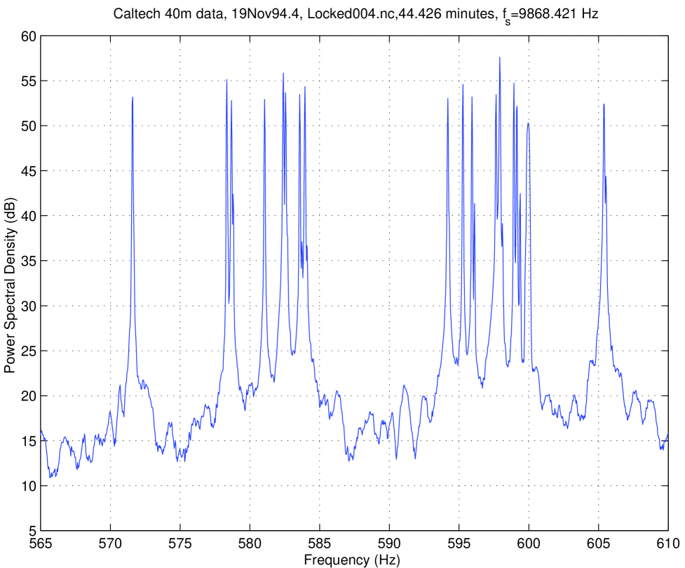
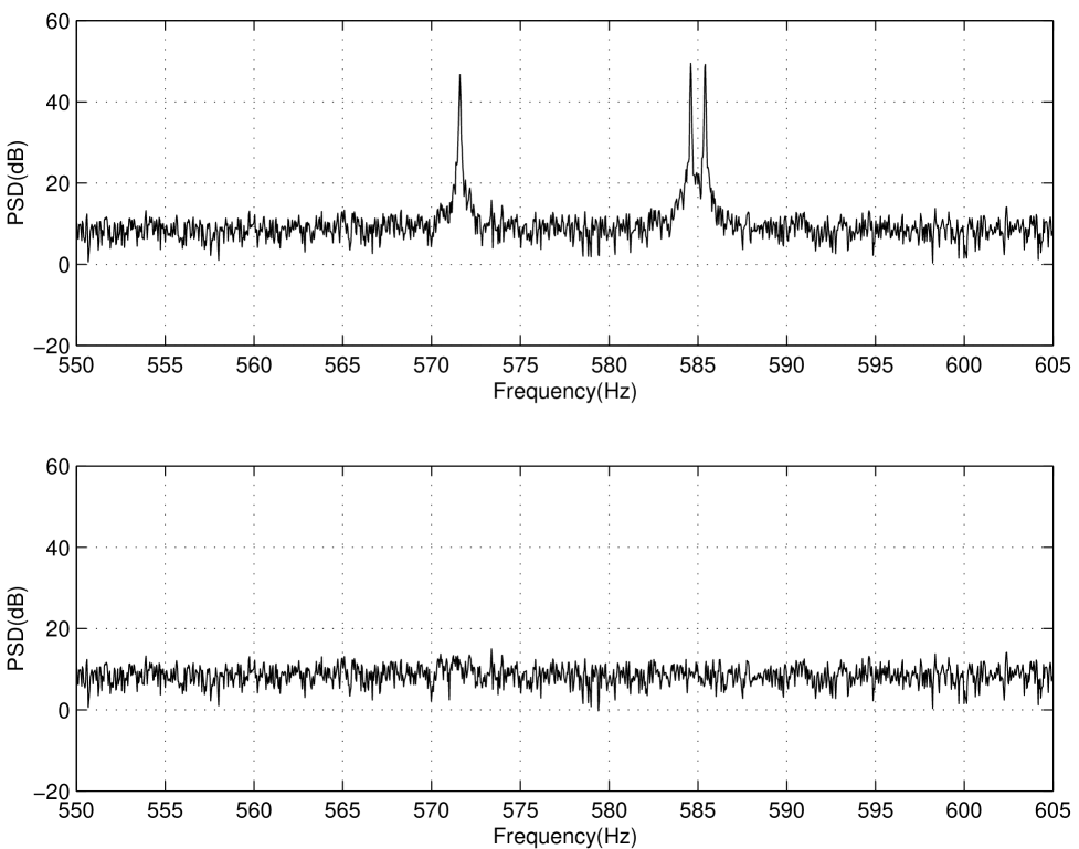
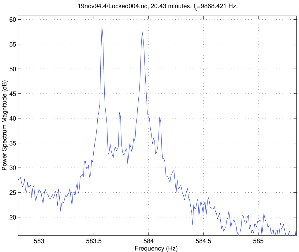
To minimize the impact of the thermal noise on the detector’s performance the suspensions are designed to have high $Q$. Laser shot noise dominates the detector noise power in a broad band about the violin mode resonant frequencies: only the peaks of the stochastically excited violin modes stand above this background. The peaks are strong, however: in the LIGO 40 M prototype they stand approximately 50 dB above the shot-noise floor and the contrast in the LIGO I detector will be approximately the same. In the LIGO 40 M prototype the fundamental violin mode resonant frequencies are in the (570, 606) Hz band with $Q$’s on order several times $10^{4}$, while in the LIGO I interferometer the fundamental violin modes will have frequencies near 330 Hz and $Q$’s on order $10^{5}$ [15]. Figure 1 shows the power spectral density (PSD) of the differential-mode read-out (IFO_DMRO) of the LIGO 40 M prototype interferometer in the neighborhood of the violin mode resonances for a typical stretch of data taken during November 1994. The units of the PSD are ADC-counts²/Hz. The line at 600 Hz is the ninth harmonic of the omnipresent 60 Hz power-main. Note how the violin mode resonances stand-out as sharp peaks some 40 dB above an approximately white (over this bandwidth) background, as described.

The combination of violin modes in an approximately white background maps naturally onto a model involving a stochastically driven dynamical process observed in the presence of white measurement noise:

• Each violin mode corresponds to a distinct dynamical processes driven by an independent noise source (thermal or otherwise);

• The observable is the motion of the cavity mirror as reflected in the gravity-wave channel of the interferometer;

• The measurement noise is the laser shot-noise, and other technical noises that affect the gravity-wave channel but do not drive the violin modes.

In the remainder of this section we describe how we restrict attention to the narrow band surrounding the violin mode, where the model associated with the use of a Kalman filter is particularly apt, and develop the state-space equations that describe the modes in that band.

B The Observations

The violin mode resonances are very weakly damped; so, the noise power in the modes contributes significantly to the overall detector output only in a very narrow band about each mode’s resonant frequency. Correspondingly, to monitor one or more violin modes we focus attention on a narrow band in the the neighborhood of the mode resonant frequencies. For definiteness, denote the gravitational wave channel at full bandwidth (sample rate $f_{s}$) by $g$ and let the band of interest, which includes the mode frequency $f_{0}$, range from $f_{c}-\Delta f/2$ to $f_{c}+\Delta f/2$, for $\Delta f$ much less than $f_{c}$.

To exploit the narrow bandwidth of the violin modes we form the complex quantity

$$g^{\prime}[k]=\exp\left(-2\pi ik{f_{c}\over f_{s}}\right)g[k].$$ (47)

The spectrum of $g^{\prime}$ in the band $[-\Delta f/2,\Delta f/2]$ is equal to the spectrum of $g$ in the band $[f_{c}-\Delta f/2,f_{c}+\Delta f/2]$. Focus attention on just this narrow band by down-sampling $g^{\prime}$ to the new sample rate $2\Delta f$ using, e.g., a polyphase technique [16, Chapter 4]. Denote the down-sampled $g^{\prime}$ by $z$, which is complex-valued.

From $z$, it is convenient to construct the real vector sequence $\mathchoice{{\hbox{\boldmath$\displaystyle z$}}}{{\hbox{\boldmath$\textstyle z$}}}{{\hbox{\boldmath$\scriptstyle z$}}}{{\hbox{\boldmath$\scriptscriptstyle z$}}}[k]$:

$$\mathchoice{{\hbox{\boldmath$\displaystyle z$}}}{{\hbox{\boldmath$\textstyle z$}}}{{\hbox{\boldmath$\scriptstyle z$}}}{{\hbox{\boldmath$\scriptscriptstyle z$}}}[k]=\left(\begin{array}[]{c}\Re(z)[k]\\ \Im(z)[k]\end{array}\right).$$ (48)

The vector-valued time series $\mathchoice{{\hbox{\boldmath$\displaystyle z$}}}{{\hbox{\boldmath$\textstyle z$}}}{{\hbox{\boldmath$\scriptstyle z$}}}{{\hbox{\boldmath$\scriptscriptstyle z$}}}[k]$ plays the role of the observation in our Kalman filter implementation.

C Dynamical Model

The gravitational wave channel $g$ is the sum of the violin modes (whose behavior we wish to determine) and other noise sources. In constructing $\textstyle z$ we focused attention on a narrow band about the mode resonant frequencies. Here we provide a model for the mode behavior as reflected in $\textstyle z$.

We first note that, near resonance, the details of the damping are unimportant; consequently, we can model each violin mode as an independent, viscously damped harmonic oscillator whose coordinate $u$ is the amplitude of the mode present in the detector output. The coordinate $u$ satisfies the differential equation

$$\ddot{u}+{\omega_{0}\over Q}\dot{u}+\omega_{0}^{2}u=F(t),$$ (49)

where $F$ is the (stochastic) driving force. The “gravity-wave” channel is the sum of $u$ and other noises (and signals).

We can relate $u$ to the contribution of the violin modes to $\textstyle z$ by mixing $u$ with the phase factor $\exp(-i\omega_{c}t)$ (where $\omega_{c}$ is equal to $2\pi f_{c}$):

$$\psi=u\exp(-i\omega_{c}t).$$ (50)

The complex $\psi$ satisfies the differential equation

$$\ddot{\psi}+\left({\omega_{0}\over Q}+2i\omega_{c}\right)\dot{\psi}+\left(\omega_{0}^{2}-\omega_{c}^{2}+i{\omega_{c}\omega_{0}\over Q}\right)\psi=F\exp(-i\omega_{c}t),$$ (52)

or, in the Laplace domain,

$$\left(s-p_{{}+{}}\right)\left(s-p_{{}-{}}\right)\bar{\psi}(s)=\bar{F}(s+i\omega_{c})$$ (53)

where

$$\bar{g}(s) = \int_{-\infty}^{\infty}dt\,\exp(-st)\,g(t)$$ (54)

$$p_{\pm} = -{\omega_{0}\over 2Q}-i\omega_{c}\pm i\omega_{0}\sqrt{1-{1\over 4Q^{2}}}.$$ (55)

(Note that in equations 50 we have assumed that $\psi$ is causal — i.e., it vanishes at sufficiently earlier times — and used a two-sided Laplace transform. Written in this way the Laplace transform $\bar{\psi}$ of $\psi$ is related to its Fourier transform $\tilde{\psi}$ through the substitution of $2\pi if$ for $s$:

$$\tilde{g}(f):=\int_{-\infty}^{\infty}dt\,\exp(-2\pi ift)\,g(t).$$ (56)

(Note that we have adopted the engineering convention for the Fourier transform.) After down-sampling, the real and imaginary parts of $\psi$ are the contributions of the violin modes to the real and imaginary parts of $\textstyle z$.

The two poles $p_{\pm}$ in the Laplace transform solution $\bar{\psi}(s)$ correspond to the positive and negative frequency resonances of the oscillator. When we choose $\omega_{c}$ close to $\omega_{0}$ we placed one of the resonances in $\psi$ near zero angular frequency and the other far away: correspondingly, one of the poles $p_{\pm}$ is near the origin and one is distant. Letting $p_{+}$ be the “near” pole and $p_{-}$ be the “far” pole we write

$$\left(s-p_{+}\right)\bar{\psi}(s)={\bar{F}(s+i\omega_{c})\over s-p_{-}},$$ (57)

or, for $|s|\ll|p_{{}-{}}|$,

$$\left(s-p_{+}\right)\bar{\psi}(s)=-p_{-}^{-1}\bar{F}(s+i\omega_{c}).$$ (58)

The spectrum of $\psi$ arising from this second equation, which differs from the first only by the source term, is identical to the spectrum of $\psi$ arising from the first as long as $|\omega|$ is much less than $|p_{-}|$. Since down-sampling restricts the bandwidth of $\psi$ in just this way we adopt equation 58 as the evolution equation for $\psi$. Correspondingly, near zero angular frequency $\psi$ satisfies

$$\dot{\psi}-p_{+}\psi=-p_{-}^{-1}F(t)e^{-i\omega_{c}t}.$$ (59)

Now write, instead of the complex $\psi$, the real vector $\textstyle\psi$ whose components are the real and imaginary parts of $\psi$:

$$\mathchoice{{\hbox{\boldmath$\displaystyle\psi$}}}{{\hbox{\boldmath$\textstyle\psi$}}}{{\hbox{\boldmath$\scriptstyle\psi$}}}{{\hbox{\boldmath$\scriptscriptstyle\psi$}}}=\left(\begin{array}[]{c}\Re(\psi)\\ \Im(\psi)\end{array}\right).$$ (60)

The first order differential equation 59 describing complex $\psi$ near zero frequency becomes a coupled set of first order differential equations

$$\dot{\mathchoice{{\hbox{\boldmath$\displaystyle\psi$}}}{{\hbox{\boldmath$\textstyle\psi$}}}{{\hbox{\boldmath$\scriptstyle\psi$}}}{{\hbox{\boldmath$\scriptscriptstyle\psi$}}}}=\mathchoice{{\hbox{\boldmath$\displaystyle A^{\prime}$}}}{{\hbox{\boldmath$\textstyle A^{\prime}$}}}{{\hbox{\boldmath$\scriptstyle A^{\prime}$}}}{{\hbox{\boldmath$\scriptscriptstyle A^{\prime}$}}}\cdot\mathchoice{{\hbox{\boldmath$\displaystyle\psi$}}}{{\hbox{\boldmath$\textstyle\psi$}}}{{\hbox{\boldmath$\scriptstyle\psi$}}}{{\hbox{\boldmath$\scriptscriptstyle\psi$}}}+\mathchoice{{\hbox{\boldmath$\displaystyle F$}}}{{\hbox{\boldmath$\textstyle F$}}}{{\hbox{\boldmath$\scriptstyle F$}}}{{\hbox{\boldmath$\scriptscriptstyle F$}}}$$ (62)

where

$$A^{\prime} = \left(\begin{array}[]{cc}\Re(p_{+})&-\Im(p_{+})\\ \Im(p_{+})&\Re(p_{+})\end{array}\right)$$ (65)

$$F = F\left(\begin{array}[]{c}\Re(p_{-}^{-1}e^{-i\omega_{c}t})\\ \Im(p_{-}^{-1}e^{-i\omega_{c}t})\end{array}\right).$$ (68)

Our observation is not of continuous $z(t)$ but of sampled $\mathchoice{{\hbox{\boldmath$\displaystyle z$}}}{{\hbox{\boldmath$\textstyle z$}}}{{\hbox{\boldmath$\scriptstyle z$}}}{{\hbox{\boldmath$\scriptscriptstyle z$}}}[k]$. Suppose that the final sampling rate is $\Delta f$ and approximate the evolution of $\textstyle\psi$ as free between samples, with the accumulated effect of the stochastic force $\textstyle F$ acting at the sample times. Then the sampled $\mathchoice{{\hbox{\boldmath$\displaystyle\psi$}}}{{\hbox{\boldmath$\textstyle\psi$}}}{{\hbox{\boldmath$\scriptstyle\psi$}}}{{\hbox{\boldmath$\scriptscriptstyle\psi$}}}[k]$ satisfies

$$\mathchoice{{\hbox{\boldmath$\displaystyle\psi$}}}{{\hbox{\boldmath$\textstyle\psi$}}}{{\hbox{\boldmath$\scriptstyle\psi$}}}{{\hbox{\boldmath$\scriptscriptstyle\psi$}}}[k]=\mathchoice{{\hbox{\boldmath$\displaystyle A$}}}{{\hbox{\boldmath$\textstyle A$}}}{{\hbox{\boldmath$\scriptstyle A$}}}{{\hbox{\boldmath$\scriptscriptstyle A$}}}\cdot\mathchoice{{\hbox{\boldmath$\displaystyle\psi$}}}{{\hbox{\boldmath$\textstyle\psi$}}}{{\hbox{\boldmath$\scriptstyle\psi$}}}{{\hbox{\boldmath$\scriptscriptstyle\psi$}}}[k-1]+\mathchoice{{\hbox{\boldmath$\displaystyle w$}}}{{\hbox{\boldmath$\textstyle w$}}}{{\hbox{\boldmath$\scriptstyle w$}}}{{\hbox{\boldmath$\scriptscriptstyle w$}}}[k]$$ (70)

where

$$\mathchoice{{\hbox{\boldmath$\displaystyle A$}}}{{\hbox{\boldmath$\textstyle A$}}}{{\hbox{\boldmath$\scriptstyle A$}}}{{\hbox{\boldmath$\scriptscriptstyle A$}}}=\exp\left(\mathchoice{{\hbox{\boldmath$\displaystyle A$}}}{{\hbox{\boldmath$\textstyle A$}}}{{\hbox{\boldmath$\scriptstyle A$}}}{{\hbox{\boldmath$\scriptscriptstyle A$}}}^{\prime}\over\Delta f\right)$$ (71)

and $\mathchoice{{\hbox{\boldmath$\displaystyle w$}}}{{\hbox{\boldmath$\textstyle w$}}}{{\hbox{\boldmath$\scriptstyle w$}}}{{\hbox{\boldmath$\scriptscriptstyle w$}}}[k]$ is a random vector related to $\textstyle F$. The quantity $\mathchoice{{\hbox{\boldmath$\displaystyle\psi$}}}{{\hbox{\boldmath$\textstyle\psi$}}}{{\hbox{\boldmath$\scriptstyle\psi$}}}{{\hbox{\boldmath$\scriptscriptstyle\psi$}}}[k]$ in this case is equal to the contribution of the violin mode to the observable $\mathchoice{{\hbox{\boldmath$\displaystyle z$}}}{{\hbox{\boldmath$\textstyle z$}}}{{\hbox{\boldmath$\scriptstyle z$}}}{{\hbox{\boldmath$\scriptscriptstyle z$}}}[k]$, or

$$\mathchoice{{\hbox{\boldmath$\displaystyle z$}}}{{\hbox{\boldmath$\textstyle z$}}}{{\hbox{\boldmath$\scriptstyle z$}}}{{\hbox{\boldmath$\scriptscriptstyle z$}}}[k]=\mathchoice{{\hbox{\boldmath$\displaystyle C$}}}{{\hbox{\boldmath$\textstyle C$}}}{{\hbox{\boldmath$\scriptstyle C$}}}{{\hbox{\boldmath$\scriptscriptstyle C$}}}\cdot\mathchoice{{\hbox{\boldmath$\displaystyle\psi$}}}{{\hbox{\boldmath$\textstyle\psi$}}}{{\hbox{\boldmath$\scriptstyle\psi$}}}{{\hbox{\boldmath$\scriptscriptstyle\psi$}}}[k]+\mathchoice{{\hbox{\boldmath$\displaystyle v$}}}{{\hbox{\boldmath$\textstyle v$}}}{{\hbox{\boldmath$\scriptstyle v$}}}{{\hbox{\boldmath$\scriptscriptstyle v$}}}[k],$$ (72)

where $\textstyle v$ represents the (approximately) white background in which the violin modes are immersed. Equations III C are the state-space form of the Kalman equations. To complete our description of the suspension modes in this form it remains to determine the properties of the process and measurement noises $\textstyle w$ and $\textstyle v$.

The statistical properties of $\textstyle w$ derive ultimately from the statistical properties of the force $F$ (cf. 49). In applying the Kalman filter we assume that $\textstyle w$, and consequently $F$, is white. Assuming that modes are driven principally by thermal forces we can use the Fluctuation-dissipation theorem [17] to find the power spectrum of the thermal force driving the mode:

$$S_{F}(f)=4k_{B}T\Re(Z)$$ (73)

where $Z$ is the system’s impedance. In our application,

$$Z={-\omega^{2}+i\gamma\omega-\omega_{0}^{2}\over i\gamma\omega};$$ (74)

so, $\Re(Z)$ is independent of frequency, the thermal force acting on the modes is white, and the assumption made in applying the Kalman filter to this problem is satisfied exactly.

The quantity $\textstyle v$ is the measurement noise: i.e., the noise within which the violin mode signal is embedded. In our application the measurement noise is associated with the laser shot noise. In the current generation of large detectors the shot noise has the spectrum

$$S_{h}(f)=S_{0}\left[1+\left(f\over f_{k}\right)^{2}\right],$$ (75)

with knee frequency $f_{k}$ approximately 100 Hz. the LIGO 40 M prototype the mode fundamental frequencies are confined to an approximately 40 Hz bandwidth about 590 Hz; in the LIGO I detector they will be in a similarly narrow band about 350 Hz. As long as we are able to confine attention to bandwidths small compared to the mode frequency the shot noise in that band will be very nearly white; correspondingly, $\textstyle v$ will be white and have a covariance $\textstyle V$ proportional to the unity matrix.

To summarize, we construct the observable $\textstyle z$ from the gravitational wave channel $g$ by mixing it with a local oscillator and down-sampling to the bandwidth $\Delta f$ about zero frequency. We model the sampled observable as arising from the equations

$$\mathchoice{{\hbox{\boldmath$\displaystyle\psi$}}}{{\hbox{\boldmath$\textstyle\psi$}}}{{\hbox{\boldmath$\scriptstyle\psi$}}}{{\hbox{\boldmath$\scriptscriptstyle\psi$}}}[k] = \mathchoice{{\hbox{\boldmath$\displaystyle A$}}}{{\hbox{\boldmath$\textstyle A$}}}{{\hbox{\boldmath$\scriptstyle A$}}}{{\hbox{\boldmath$\scriptscriptstyle A$}}}\cdot\mathchoice{{\hbox{\boldmath$\displaystyle\psi$}}}{{\hbox{\boldmath$\textstyle\psi$}}}{{\hbox{\boldmath$\scriptstyle\psi$}}}{{\hbox{\boldmath$\scriptscriptstyle\psi$}}}[k-1]+\mathchoice{{\hbox{\boldmath$\displaystyle v$}}}{{\hbox{\boldmath$\textstyle v$}}}{{\hbox{\boldmath$\scriptstyle v$}}}{{\hbox{\boldmath$\scriptscriptstyle v$}}}[k-1]$$ (77)

$$\mathchoice{{\hbox{\boldmath$\displaystyle z$}}}{{\hbox{\boldmath$\textstyle z$}}}{{\hbox{\boldmath$\scriptstyle z$}}}{{\hbox{\boldmath$\scriptscriptstyle z$}}}[k] = \mathchoice{{\hbox{\boldmath$\displaystyle C$}}}{{\hbox{\boldmath$\textstyle C$}}}{{\hbox{\boldmath$\scriptstyle C$}}}{{\hbox{\boldmath$\scriptscriptstyle C$}}}\cdot\mathchoice{{\hbox{\boldmath$\displaystyle\psi$}}}{{\hbox{\boldmath$\textstyle\psi$}}}{{\hbox{\boldmath$\scriptstyle\psi$}}}{{\hbox{\boldmath$\scriptscriptstyle\psi$}}}[k]+\mathchoice{{\hbox{\boldmath$\displaystyle w$}}}{{\hbox{\boldmath$\textstyle w$}}}{{\hbox{\boldmath$\scriptstyle w$}}}{{\hbox{\boldmath$\scriptscriptstyle w$}}}[k]$$ (78)

where

$$A = \exp\left({\mathchoice{{\hbox{\boldmath$\displaystyle A$}}}{{\hbox{\boldmath$\textstyle A$}}}{{\hbox{\boldmath$\scriptstyle A$}}}{{\hbox{\boldmath$\scriptscriptstyle A$}}}^{\prime}\over\Delta f}\right)$$ (79)

$$\mathchoice{{\hbox{\boldmath$\displaystyle A$}}}{{\hbox{\boldmath$\textstyle A$}}}{{\hbox{\boldmath$\scriptstyle A$}}}{{\hbox{\boldmath$\scriptscriptstyle A$}}}^{\prime} = \left(\begin{array}[]{cc}-{\omega_{0}/2Q}&\omega_{c}-\omega_{0}\sqrt{1-{1/4Q^{2}}}\\ -\omega_{c}+\omega_{0}\sqrt{1-{1/4Q^{2}}}&-{\omega_{0}/2Q}\end{array}\right)$$ (82)

D Reconstruction

In applying the Kalman filter we determine, at each sample, the state estimate $\widehat{\mathchoice{{\hbox{\boldmath$\displaystyle\psi$}}}{{\hbox{\boldmath$\textstyle\psi$}}}{{\hbox{\boldmath$\scriptstyle\psi$}}}{{\hbox{\boldmath$\scriptscriptstyle\psi$}}}}[k]$ from which we form an estimate $\widehat{\mathchoice{{\hbox{\boldmath$\displaystyle z$}}}{{\hbox{\boldmath$\textstyle z$}}}{{\hbox{\boldmath$\scriptstyle z$}}}{{\hbox{\boldmath$\scriptscriptstyle z$}}}}_{v}$ of the contribution of the violin mode to the detector output:

$$\widehat{\mathchoice{{\hbox{\boldmath$\displaystyle z$}}}{{\hbox{\boldmath$\textstyle z$}}}{{\hbox{\boldmath$\scriptstyle z$}}}{{\hbox{\boldmath$\scriptscriptstyle z$}}}}_{v}=\mathchoice{{\hbox{\boldmath$\displaystyle C$}}}{{\hbox{\boldmath$\textstyle C$}}}{{\hbox{\boldmath$\scriptstyle C$}}}{{\hbox{\boldmath$\scriptscriptstyle C$}}}\cdot\widehat{\mathchoice{{\hbox{\boldmath$\displaystyle\psi$}}}{{\hbox{\boldmath$\textstyle\psi$}}}{{\hbox{\boldmath$\scriptstyle\psi$}}}{{\hbox{\boldmath$\scriptscriptstyle\psi$}}}}.$$ (83)

The violin mode contribution to the observation is an instrumental artifact that is unrelated to the incidence of gravitational waves on the detector; correspondingly, we may wish to use the prediction to subtractively remove the artifact from the data stream.

The prediction $\widehat{\mathchoice{{\hbox{\boldmath$\displaystyle z$}}}{{\hbox{\boldmath$\textstyle z$}}}{{\hbox{\boldmath$\scriptstyle z$}}}{{\hbox{\boldmath$\scriptscriptstyle z$}}}}_{v}$ for the violin mode contribution is formed at reduced bandwidth and offset frequency. From $\widehat{\mathchoice{{\hbox{\boldmath$\displaystyle z$}}}{{\hbox{\boldmath$\textstyle z$}}}{{\hbox{\boldmath$\scriptstyle z$}}}{{\hbox{\boldmath$\scriptscriptstyle z$}}}}_{v}$ we can construct the predicted contribution violin mode contribution to the full bandwidth observation ($g[k]$, cf. 47) by reversing the steps taken to form $\textstyle z$ from $g$ (cf. sec. III B). In particular, we first form the complex scalar sequence

$$\widehat{z}_{v}=\left(\begin{array}[]{cc}1&i\end{array}\right)\cdot\widehat{\mathchoice{{\hbox{\boldmath$\displaystyle z$}}}{{\hbox{\boldmath$\textstyle z$}}}{{\hbox{\boldmath$\scriptstyle z$}}}{{\hbox{\boldmath$\scriptscriptstyle z$}}}}_{v}$$ (84)

and up-sample it to the full sample rate, forming $\widehat{G}^{\prime}_{v}$. The mixing operation undertaken in equation 47 can then be reversed,

$$\widehat{G}_{v}[k]=\widehat{G}^{\prime}[k]\exp\left(2\pi ik{f_{c}\over f_{s}}\right).$$ (85)

The result is still complex: it is missing the contributions from negative frequencies that were discarded in the low-pass filtering that accompanied the original down-sampling operation. Since the original observation was real, however, this contribution is just the complex conjugate of the positive frequency contribution, which we have; consequently, the estimated contribution of the violin mode to the data stream $g[k]$ is

$$\widehat{g}_{v}[k]=2\Re(\widehat{G}[k]).$$ (86)

The residual difference

$$g_{r}[k]=g[k]-\widehat{g}_{v}[k]$$ (87)

is then free of violin mode artifact, to the accuracy of our estimation procedure.

E Estimating the measurement and process noise

To use the Kalman filter we must have a model for the process dynamics ($\textstyle A$) and how the process contributes to the observable ($\textstyle C$). These we described for our particular application — the violin modes of an interferometer mirror suspensions (each mode an independent process) — in section III B. Additionally, we must have estimates for the process and measurement noise co-variance matrices ($\textstyle W$ and $\textstyle V$). Here we describe how we estimate these from a short segment of filter input, taken at the beginning of the input.

Consider the typical bandwidth of the observable $\textstyle z$, shown in figure 1. The process contributes significantly over only a small fraction of the bandwidth, where the resonance rises above the measurement noise floor. To estimate the measurement noise, we form the PSD of $z$ and take the average power far from the resonant peaks. This average power $\overline{P}_{m}$ is the total measurement noise (tr $\textstyle V$). We assume that there is no cross-covariance between the noise in $\Re(z)$ and $\Im(z)$, in which case

$$\mathchoice{{\hbox{\boldmath$\displaystyle V$}}}{{\hbox{\boldmath$\textstyle V$}}}{{\hbox{\boldmath$\scriptstyle V$}}}{{\hbox{\boldmath$\scriptscriptstyle V$}}}={1\over 2}\overline{P}_{m}\,\left(\begin{array}[]{cc}1&0\\ 0&1\end{array}\right).$$ (88)

To estimate the process noise we focus on that part of the spectrum near the resonant peak where the process dominates. We assume, in our model, that the process is driven by white noise. From the Kalman filter model, the power spectral density of the contribution to $z$ in this bandwidth is given by (cf. equation 59)

$$P_{z}(\omega)={4Q^{2}\text{tr}\,\mathchoice{{\hbox{\boldmath$\displaystyle W$}}}{{\hbox{\boldmath$\textstyle W$}}}{{\hbox{\boldmath$\scriptstyle W$}}}{{\hbox{\boldmath$\scriptscriptstyle W$}}}\over\omega_{0}^{2}+\left(2Q\omega_{c}-\omega_{0}\left(4Q^{2}-1\right)^{1/2}\right)^{2}}.$$ (89)

With the exception of the total process noise (tr $\textstyle W$) the right hand side of equation 89 is known. The left hand side we measure. To estimate tr$\textstyle W$, we measure $P_{z}$ and sum it over the limited bandwidth dominated by the process. Setting that equal to the same sum executed on the right hand side of equation 89 we determine the proportionality constant tr $\textstyle W$. Assuming that the process noise is equally distributed between the real and imaginary parts of $\textstyle z$, with no cross-variance, we thus determine the estimated process noise covariance:

$$\mathchoice{{\hbox{\boldmath$\displaystyle W$}}}{{\hbox{\boldmath$\textstyle W$}}}{{\hbox{\boldmath$\scriptstyle W$}}}{{\hbox{\boldmath$\scriptscriptstyle W$}}}={1\over 2}\left(\text{tr}\,\mathchoice{{\hbox{\boldmath$\displaystyle W$}}}{{\hbox{\boldmath$\textstyle W$}}}{{\hbox{\boldmath$\scriptstyle W$}}}{{\hbox{\boldmath$\scriptscriptstyle W$}}}\right)\left(\begin{array}[]{cc}1&0\\ 0&1\end{array}\right).$$ (90)

IV Characterization

Before providing results from the application of our filter on LIGO 40 M prototype data we characterize the filter’s behavior on “synthetic” or “mock” time series. These time series are constructed so that the violin mode state, process noise, measurement noise, and signal content are known exactly. By applying the filter to these data sets and investigating the difference between its estimation of these quantities and their actual, known values, we characterize the filter’s performance.

Four applications to synthetic data sets are described here:

1. A single isolated violin mode, driven by Gaussian white process noise and observed in the presence of Gaussian white measurement noise (cf.s̃ec. IV B);

2. Several closely spaced violin modes, driven by non-Gaussian white process noise and observed in the presence of non-Gaussian white measurement noise (cf. sec. IV C);

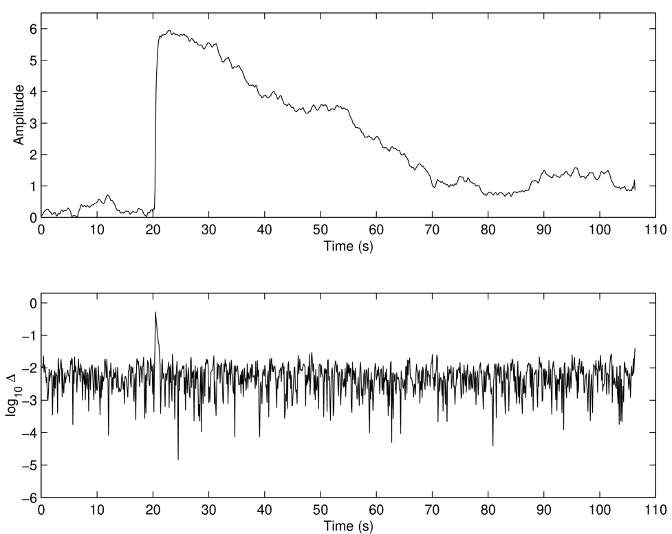
3. A single isolated violin mode, driven by Gaussian white process noise with a superposed impulsive excitation and observed in the presence of non-Gaussian white measurement noise (cf. sec. IV D); and

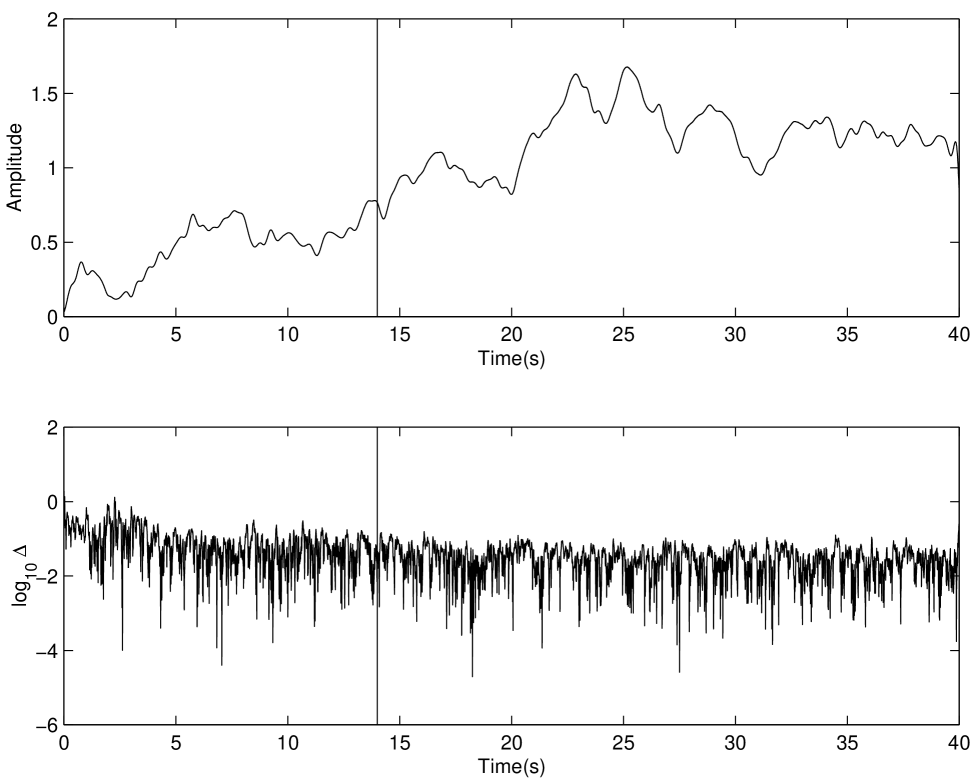
4. A single isolated violin mode, driven by non-Gaussian white process noise and observed in the presence of non-Gaussian white measurement noise with a superposed impulsive excitation (cf. sec. IV E).

The first case demonstrates the filter operating in the regime where the measurement noise and process noise satisfy the assumptions made in the derivation of the Kalman filter. The second case examines the filter’s ability to distinguish a violin mode from measurement noise, and to distinguish between two different modes, when the noise is not as simple as Gaussian and modes are closely spaced in frequency. In the third case we test the filter’s ability to respond to impulsive excitations of the suspension modes. In the final case we introduce an impulse into the measurement noise and observe the filter’s ability to discriminate between it and the contribution from the violin mode.

As they appear in the detector data stream, violin modes are characterized entirely by their resonant frequency $f_{0}$ and damping constant $Q$. Since we are dealing always with discrete-time signal processing, the scale of the frequency does not matter: the only relevant quantity (aside from $Q$) is the ratio of the resonant frequency to the sampling frequency $f_{s}$. Nevertheless, to foreshadow our application of the filter to data taken at the LIGO 40 M prototype, we assume that the sampling frequency is 9868.421 Hz, the sampling rate of the LIGO 40 M prototype, and we always choose the simulated violin modes to have resonant frequencies coincident with the frequencies of modes identified in that instrument. With this convention, the frequency and damping constants of the simulated modes used in the examples to follow are given in table I.

A Generating synthetic data sets

Before discussing the results of our investigations into the Kalman filter’s behavior we describe how we generated the random time series used in those investigations.

In all cases the measurement noise is white: i.e., its power spectrum was constant over its bandwidth. For Gaussian noise measurement noise we used Matlab’s [18] randn random number generator. Non-Gaussian noise was modeled by a two-component mixture-Gaussian model:

$$P(x|\alpha,\mu_{1},\mu_{2},\sigma_{1},\sigma_{2}) = \alpha N(\mu_{1},\sigma_{1})+\left(1-\alpha\right)N(\mu_{2},\sigma_{2})$$ (92)

$$\begin{array}[]{rclcrcl}\alpha&=&0.7,&&&&\\ \mu_{1}&=&0,&&\mu_{2}&=&0,\\ \sigma_{1}&=&1,&&\sigma_{2}&=&1.5.\end{array}$$ (96)

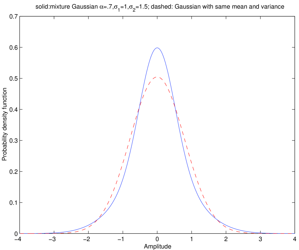
Here $N(\mu,\sigma)$ represents a Normal process with mean $\mu$ and variance $\sigma^{2}$, the parameters $\alpha$, $\mu_{k}$ and $\sigma_{k}$ are fixed with $0\leq\alpha\leq 1$. Figure 2 shows the distribution of this mixture Gaussian process together with the distribution of a Gaussian process with the same mean and variance. The mixture Gaussian distribution described by the parameters in equation IV A is strongly leptokurtic (i.e., it has a significant excess of high amplitude events).

To generate the contribution to the observation from the process we begin with the differential equation modeling the process (cf. 49):

$$\ddot{r}+{\omega_{0}\over Q}\dot{r}+\omega_{0}^{2}r=F,$$ (97)

where $r$ is the position of the suspended mass. We make no assumptions here about driving force $F$. The detector gravitational wave channel consists of a superposition of measurement noise $v$ and the oscillator coordinate $r$. The solution to this equation can be expressed as an all-pole linear filter $H$ acting on the driving force $F$. In the Laplace domain the filter is given by

$$\bar{r}(s) = \bar{H}(s)\bar{F}(s)$$ (99)

$$\bar{H}(s) = {1\over s^{2}+s\omega_{0}/Q+\omega_{0}^{2}}$$ (100)

$$= {1\over\left(s-p_{+}\right)\left(s-p_{-}\right)}$$ (101)

where

$$p_{\pm}=-\left(\omega_{0}/2Q\pm i\omega_{0}\sqrt{1-1/4Q^{2}}\right)$$ (102)

The frequency response of the filter at angular frequency $\omega$ is equal to $\bar{H}(s)$ evaluated on the imaginary axis:

$$\widetilde{H}(\omega)=\bar{H}(i\omega).$$ (103)

The two-pole filter $H$ operates in continuous time while the detector output we wish to simulate is discretely sampled at a rate $f_{s}$, which we assume is at least twice as great as the resonant frequency $f_{0}$. Using the analog filter $\bar{H}(s)$ as a prototype, we design a digital filter with a similar response at frequencies much less than the Nyquist frequency.

Suppose that the discretely sampled sequence $r[k]$, driven by the input $F[k]$, satisfies

$$u[k]=\sum_{j=0}^{N_{b}}b[j]F[k-j]-\sum_{j=1}^{N_{a}}a[j]u[k-j],$$ (104)

where $a[j]$ and $b[j]$ are the constant filter coefficients. Define the $z$-transform of the sequence $y[k]$ by

$$\check{y}\equiv\sum_{k=-\infty}^{\infty}y[k]z^{-k}.$$ (105)

(The $z$-transform of a digital filter is analogous to the Laplace transform of a continuous filter.) In $z$-space, the linear filter described in equation 104 can be written

$$\check{r}(z) = {\sum_{j=0}^{N_{b}}b[j]z^{-j}\over 1+\sum_{j=1}^{N_{a}}a[j]z^{-j}}\check{F}(z)$$ (107)

$$= \check{G}(z)\check{F}(z)$$ (108)

The frequency response of the digital filter $G$ is equal to $\check{G}(z)$ evaluated on the unit circle in the complex $z$-plane:

$$\check{G}\left(e^{2\pi if/f_{s}}\right)$$ (109)

where $f_{s}$ is the sample rate of the filtered sequence. If, by a conformal transformation, we map the right half $s$-plane on to the interior of the unit circle in the $z$-plane, then we will have mapped the analog prototype $\bar{H}(s)$ on to the digital filter $\check{G}(z)$:

$$\check{G}(z)=\bar{H}(s)|_{s=2\Omega(z-1)/(z+1)},$$ (110)

where $\Omega$ is the so-called warping constant. This mapping will not be without distortion; nevertheless, at frequencies much less than the Nyquist frequency the distortion will be minimal. We can choose the warping constant $\Omega$ to guarantee that the digital filter’s response matches exactly the analog filter’s response at exactly one frequency:

$$\check{G}(e^{-2\pi if^{\prime}/f_{s}})=\bar{H}(2\pi if^{\prime})$$ (111)

when

$$\Theta={\pi f^{\prime}\over\tan(\pi f^{\prime}/f_{s})}.$$ (112)

We choose the warping constant so that the response of the digital filter matches the response of the analog filter at the resonant frequency $f_{0}$. This completes the design of the digital filter $\check{G}(z)$. Given a pseudo-random process $F[k]$ and the recursion relationship of equation 104 we evaluate $r[k]$, the simulated contribution of the violin mode to the detector output. Finally, to obtain the simulated gravitational-wave channel output, we add to $r[k]$ another pseudo-random process $n[k]$, which represents the measurement noise.

In our simulations we used the $\csc Matlab$ [18] Normal random number generatorrandn wherever Normal deviates were called for: i.e., in forming either the measurement noise, the process noise or the stochastic driving force $F$.

B Single mode: Normal, white process and measurement noise

Using the techniques described above we generated several hundred seconds of simulated data, consisting of a single mode with the frequency and damping constants given in the first column of table I. The process noise was white with variance of 2.38; the measurement noise was also white with variance 2.8.

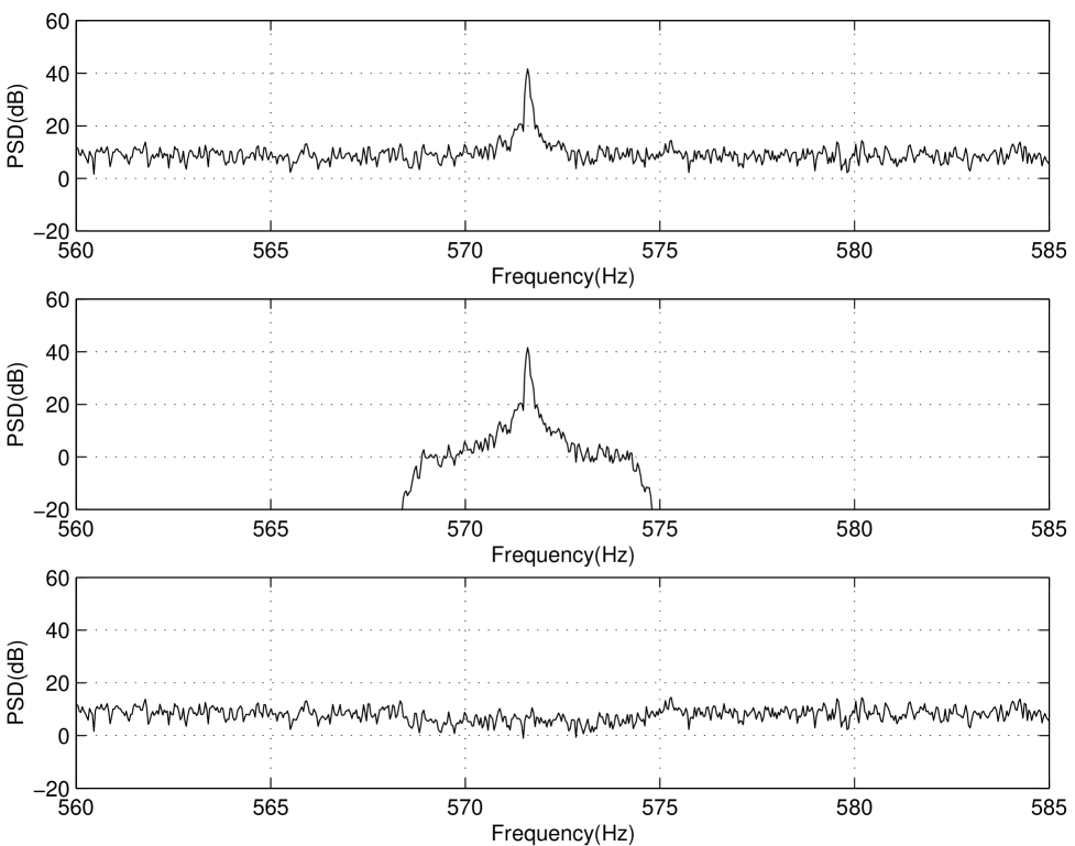
After generating the data set we applied the Kalman filter, focusing on a 6 Hz bandwidth $\Delta f$ centered about the mode’s resonant frequency. Following the discussion in section III E we estimated $\textstyle W$ and $\textstyle V$ using approximately 100 s of the simulated data. We applied the Kalman filter to the subsequent simulated data, using these values of $\textstyle W$, $\textstyle V$, setting the initial state estimate $\widehat{\mathchoice{{\hbox{\boldmath$\displaystyle\psi$}}}{{\hbox{\boldmath$\textstyle\psi$}}}{{\hbox{\boldmath$\scriptstyle\psi$}}}{{\hbox{\boldmath$\scriptscriptstyle\psi$}}}}$ to zero and the initial estimated error $\textstyle P$ equal to $\textstyle W$$\textstyle I$ (where $\textstyle I$ is the identity matrix). Figure 3 summarizes, in three panels, the Kalman filter’s effectiveness in estimating the mode state. The upper panel shows the power spectrum of the simulated observations in a wide band about the mode frequency. The middle panel shows the power spectrum of the Kalman estimate of the mode contribution to the observable. Finally, the lower panel shows the power spectral density of the difference between the actual data and the estimated contribution from the mode.. Comparing these three panels it is clear that the Kalman filter has correctly identified the modes contribution to the observable.

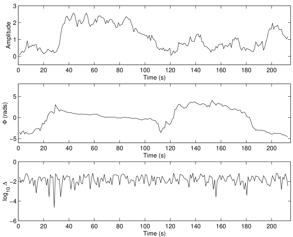
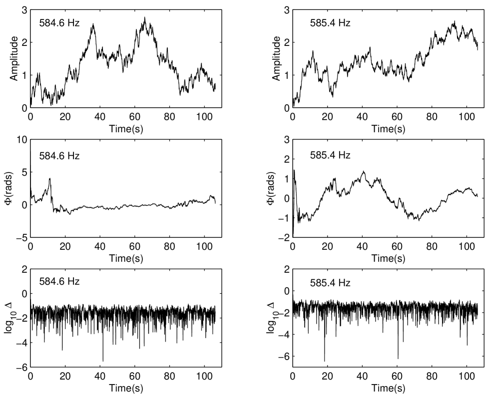
Since the data is simulated we know exactly the measurement noise and mode contributions to the observable. Correspondingly, we can evaluate the actual error in the filter’s estimate of the mode state. The mode (estimated) state is described by the complex ($\widehat{\psi}[k]$) $\psi[k]$, which we describe by its amplitude and phase

$$A := |\psi|$$ (114)

$$\tan\phi := \Im(\psi)/\Re(\psi).$$ (115)

The difference between the actual and estimated mode states we describe by the quantity $\Delta$:

$$\Delta:={2|\psi[k]-\widehat{\psi}[k]|\over|\psi[k]+\widehat{\psi}[k]|}.$$ (116)

Figure 4 shows the instantaneous estimated mode amplitude, phase and error $\Delta$. The top panel shows the estimated mode amplitude. The middle panel shows the estimate mode phase, less $2\pi f_{0}t$, where $f_{0}$ is the mode frequency. The bottom panel shows the error in the estimated mode state. Following an initial epoch, during which the filter is “locking-on” to the mode state, the relative error in the state estimate falls quickly to zero.

The middle and bottom panel of figure 3 show a slight depression in the power spectral density of the residual in the band that the Kalman filter operates. This slight depression is associated with the error in the state estimate, which is shown in the bottom panel in figure 4 to be on order several percent. The depression is uniform throughout the band, showing that the errors introduced by the subtraction of the estimated mode contribution from the data are white. For this reason it is unlikely that these errors can be reduced by, for example, a “better” estimate of $\textstyle W$, $\textstyle V$, $f_{0}$ or $Q$: changing any of these would lead to an error that was not white, but reflected either an over- or under-estimate of the power in the mode relative to the measurement error.

We expect that the continuously updated mode amplitude and phase estimates as a function of time, either analyzed directly or displayed in a strip chart of which the top two panels of figure 4 may be considered a snapshot, will be particularly useful for monitoring the state of the detector.

C Multiple modes; non-Gaussian white measurement and process noise

In deriving the Kalman filter we assumed that the process and measurement noise were white; however, we never required that they be Gaussian. Here we investigate the effectiveness of the filter when these noises are non-Gaussian and when there are several modes present, at least two of which are very close together in frequency. This is a critical application, since in actual data there are multiple closely spaced violin modes resulting from several suspension wires of the mirrors, which cannot be estimated separately (cf. 1). The mode frequencies and damping constants for this example are given in the second column of table I.

For isolated modes (i.e., those whose resonant peaks do not overlap with each other above the level of the measurement noise), one can design and apply separately a Kalman filter for each mode. Closely spaced modes cannot be treated in isolation; however, since the mode dynamics are independent, the development of a Kalman filter that treats $N$ modes jointly is straightforward:

• Referring to section III B, fix a carrier frequency $f_{c}$ and a bandwidth $\Delta f$ such that the modes of interest all have resonances in the band $[f_{c}-\Delta f/2,f_{c}+\Delta f/2]$.

• Considered separately, the dynamics of the mode $j$ ($1\leq j\leq N$) and the contribution $\mathchoice{{\hbox{\boldmath$\displaystyle z$}}}{{\hbox{\boldmath$\textstyle z$}}}{{\hbox{\boldmath$\scriptstyle z$}}}{{\hbox{\boldmath$\scriptscriptstyle z$}}}_{j}$ of the mode to the measurement are described by the equations

  $$\mathchoice{{\hbox{\boldmath$\displaystyle\psi$}}}{{\hbox{\boldmath$\textstyle\psi$}}}{{\hbox{\boldmath$\scriptstyle\psi$}}}{{\hbox{\boldmath$\scriptscriptstyle\psi$}}}_{j}[k] = \mathchoice{{\hbox{\boldmath$\displaystyle A$}}}{{\hbox{\boldmath$\textstyle A$}}}{{\hbox{\boldmath$\scriptstyle A$}}}{{\hbox{\boldmath$\scriptscriptstyle A$}}}_{j}\cdot\mathchoice{{\hbox{\boldmath$\displaystyle\psi$}}}{{\hbox{\boldmath$\textstyle\psi$}}}{{\hbox{\boldmath$\scriptstyle\psi$}}}{{\hbox{\boldmath$\scriptscriptstyle\psi$}}}_{j}[k-1]+\mathchoice{{\hbox{\boldmath$\displaystyle w$}}}{{\hbox{\boldmath$\textstyle w$}}}{{\hbox{\boldmath$\scriptstyle w$}}}{{\hbox{\boldmath$\scriptscriptstyle w$}}}_{j}[k-1]$$ (118)

  $$\mathchoice{{\hbox{\boldmath$\displaystyle z$}}}{{\hbox{\boldmath$\textstyle z$}}}{{\hbox{\boldmath$\scriptstyle z$}}}{{\hbox{\boldmath$\scriptscriptstyle z$}}}_{j}[k] = \mathchoice{{\hbox{\boldmath$\displaystyle C$}}}{{\hbox{\boldmath$\textstyle C$}}}{{\hbox{\boldmath$\scriptstyle C$}}}{{\hbox{\boldmath$\scriptscriptstyle C$}}}_{j}\cdot\mathchoice{{\hbox{\boldmath$\displaystyle\psi$}}}{{\hbox{\boldmath$\textstyle\psi$}}}{{\hbox{\boldmath$\scriptstyle\psi$}}}{{\hbox{\boldmath$\scriptscriptstyle\psi$}}}_{j}[k].$$ (119)

• The Kalman equations describing the joint evolution of the $N$ modes, and their contribution to the observation $\textstyle z$ are then

  $$\mathchoice{{\hbox{\boldmath$\displaystyle\Psi$}}}{{\hbox{\boldmath$\textstyle\Psi$}}}{{\hbox{\boldmath$\scriptstyle\Psi$}}}{{\hbox{\boldmath$\scriptscriptstyle\Psi$}}}[k] = \mathchoice{{\hbox{\boldmath$\displaystyle A$}}}{{\hbox{\boldmath$\textstyle A$}}}{{\hbox{\boldmath$\scriptstyle A$}}}{{\hbox{\boldmath$\scriptscriptstyle A$}}}\cdot\mathchoice{{\hbox{\boldmath$\displaystyle\Psi$}}}{{\hbox{\boldmath$\textstyle\Psi$}}}{{\hbox{\boldmath$\scriptstyle\Psi$}}}{{\hbox{\boldmath$\scriptscriptstyle\Psi$}}}[k-1]+\mathchoice{{\hbox{\boldmath$\displaystyle w$}}}{{\hbox{\boldmath$\textstyle w$}}}{{\hbox{\boldmath$\scriptstyle w$}}}{{\hbox{\boldmath$\scriptscriptstyle w$}}}[k-1]$$ (121)

  $$\mathchoice{{\hbox{\boldmath$\displaystyle z$}}}{{\hbox{\boldmath$\textstyle z$}}}{{\hbox{\boldmath$\scriptstyle z$}}}{{\hbox{\boldmath$\scriptscriptstyle z$}}}[k] = \mathchoice{{\hbox{\boldmath$\displaystyle C$}}}{{\hbox{\boldmath$\textstyle C$}}}{{\hbox{\boldmath$\scriptstyle C$}}}{{\hbox{\boldmath$\scriptscriptstyle C$}}}\cdot\mathchoice{{\hbox{\boldmath$\displaystyle\Psi$}}}{{\hbox{\boldmath$\textstyle\Psi$}}}{{\hbox{\boldmath$\scriptstyle\Psi$}}}{{\hbox{\boldmath$\scriptscriptstyle\Psi$}}}[k]+\mathchoice{{\hbox{\boldmath$\displaystyle v$}}}{{\hbox{\boldmath$\textstyle v$}}}{{\hbox{\boldmath$\scriptstyle v$}}}{{\hbox{\boldmath$\scriptscriptstyle v$}}}[k],$$ (122)

  where

  $$\Psi := \left(\begin{array}[]{c}\mathchoice{{\hbox{\boldmath$\displaystyle\psi$}}}{{\hbox{\boldmath$\textstyle\psi$}}}{{\hbox{\boldmath$\scriptstyle\psi$}}}{{\hbox{\boldmath$\scriptscriptstyle\psi$}}}_{1}\\ \vdots\\ \mathchoice{{\hbox{\boldmath$\displaystyle\psi$}}}{{\hbox{\boldmath$\textstyle\psi$}}}{{\hbox{\boldmath$\scriptstyle\psi$}}}{{\hbox{\boldmath$\scriptscriptstyle\psi$}}}_{N}\end{array}\right),$$ (126)

  $$= \left(\begin{array}[]{c}\Re(\psi_{1})\\ \Im(\psi_{1})\\ \vdots\\ \Re(\psi_{N})\\ \Im(\psi_{N})\end{array}\right),$$ (132)

  $$A := \left(\begin{array}[]{ccc}\mathchoice{{\hbox{\boldmath$\displaystyle A$}}}{{\hbox{\boldmath$\textstyle A$}}}{{\hbox{\boldmath$\scriptstyle A$}}}{{\hbox{\boldmath$\scriptscriptstyle A$}}}_{1}&&\\ &\ddots&\\ &&\mathchoice{{\hbox{\boldmath$\displaystyle A$}}}{{\hbox{\boldmath$\textstyle A$}}}{{\hbox{\boldmath$\scriptstyle A$}}}{{\hbox{\boldmath$\scriptscriptstyle A$}}}_{N}\end{array}\right),$$ (136)

  $$W := \left(\begin{array}[]{ccc}\mathchoice{{\hbox{\boldmath$\displaystyle W$}}}{{\hbox{\boldmath$\textstyle W$}}}{{\hbox{\boldmath$\scriptstyle W$}}}{{\hbox{\boldmath$\scriptscriptstyle W$}}}_{1}&&\\ &\ddots&\\ &&\mathchoice{{\hbox{\boldmath$\displaystyle W$}}}{{\hbox{\boldmath$\textstyle W$}}}{{\hbox{\boldmath$\scriptstyle W$}}}{{\hbox{\boldmath$\scriptscriptstyle W$}}}_{N}\end{array}\right),$$ (140)

  $$V := \left(\begin{array}[]{ccc}\mathchoice{{\hbox{\boldmath$\displaystyle V$}}}{{\hbox{\boldmath$\textstyle V$}}}{{\hbox{\boldmath$\scriptstyle V$}}}{{\hbox{\boldmath$\scriptscriptstyle V$}}}_{1}&&\\ &\ddots&\\ &&\mathchoice{{\hbox{\boldmath$\displaystyle V$}}}{{\hbox{\boldmath$\textstyle V$}}}{{\hbox{\boldmath$\scriptstyle V$}}}{{\hbox{\boldmath$\scriptscriptstyle V$}}}_{N}\end{array}\right),$$ (144)

  $$C := \left(\begin{array}[]{ccc}\mathchoice{{\hbox{\boldmath$\displaystyle C$}}}{{\hbox{\boldmath$\textstyle C$}}}{{\hbox{\boldmath$\scriptstyle C$}}}{{\hbox{\boldmath$\scriptscriptstyle C$}}}_{1}&\cdots&\mathchoice{{\hbox{\boldmath$\displaystyle C$}}}{{\hbox{\boldmath$\textstyle C$}}}{{\hbox{\boldmath$\scriptstyle C$}}}{{\hbox{\boldmath$\scriptscriptstyle C$}}}_{N}\end{array}\right)$$ (146)

  $$= \left(\begin{array}[]{ccccc}1&0&\cdots&1&0\\ 0&1&\cdots&0&1\end{array}\right),$$ (149)

  and $\mathchoice{{\hbox{\boldmath$\displaystyle W$}}}{{\hbox{\boldmath$\textstyle W$}}}{{\hbox{\boldmath$\scriptstyle W$}}}{{\hbox{\boldmath$\scriptscriptstyle W$}}}_{j}$ and $\mathchoice{{\hbox{\boldmath$\displaystyle V$}}}{{\hbox{\boldmath$\textstyle V$}}}{{\hbox{\boldmath$\scriptstyle V$}}}{{\hbox{\boldmath$\scriptscriptstyle V$}}}_{j}$ are, as before, the process and measurement noise.

In constructing $\textstyle W$ we have approximated the individual modes as being driven by independent process noise sources. Correlated process noise leads to correlations in the states of the individual modes. Even in the absence of an explicit correlation in the assumed process noise covariance (i.e., off-diagonal terms in $\textstyle W$), the filter will, if warranted by the observations, correlate the state estimates. Lacking knowledge of the driving noise (beyond contact with independent thermal baths), assuming that the process noise is uncorrelated guarantees that there is no prejudice that the mode states are correlated without constraining the state estimates to be uncorrelated.

To evaluate the effectiveness of the Kalman filter in treating multiple modes driven by non-Normal noise, we applied a single Kalman filter to this three mode system, choosing $f_{c}$ equal to 578.6 Hz and $\Delta f$ equal to 18 Hz. The top panel of figure 5 shows the power spectral density of the simulated gravity wave channel in a 60 Hz bandwidth about the carrier frequency $f_{c}$, while the bottom panel shows the power spectral density of the residual difference between the simulated observation and the filter’s prediction of the contribution from the violin modes. The residual broad feature that remains following the subtraction of the mode estimate is due to the non-Gaussian nature of the process noise that drives the mode. The filter has made a best-estimate of the mode state, given only knowledge of the driving force variance. In this example, however, the variance provides a very incomplete picture of the process noise. Still, the filter has clearly identified approximately 45 dB of the approximately 55 dB of the mode contribution to the measurement.

The state $\textstyle\Psi$ is the direct sum of the state vector estimates $\mathchoice{{\hbox{\boldmath$\displaystyle\psi$}}}{{\hbox{\boldmath$\textstyle\psi$}}}{{\hbox{\boldmath$\scriptstyle\psi$}}}{{\hbox{\boldmath$\scriptscriptstyle\psi$}}}_{j}$ of the individual modes; consequently, the filter identifies not just the total contribution of each mode to the observation, but the state of each mode separately. The four panels of figure 6 show the estimated amplitude and phase (less $2\pi f_{j}t$ for each mode) of each of the two overlapping modes at 584.6 Hz ($f_{2}$) and 585.4 Hz ($f_{3}$). In this example the two modes are known to be uncorrelated; consequently, we expect that the state estimates should also be uncorrelated, which we have found to be the case.

D Effect of a transient excitation of a mode

To evaluate the effectiveness of the Kalman filter in estimating the filter state in the presence of a transient excitation, we have simulated a single mode observed in the presence of the same mixture-Gaussian measurement noise described above (cf. equation IV A). The process noise is taken to be Gaussian with variance 2.38. At 20 seconds into the simulation we add to the process noise a single pulse of magnitude $35\sigma$, where $\sigma$ is the rms amplitude of the process noise. The top panel of figure 7 shows the estimated amplitude of the mode while the bottom panel shows error $\Delta$ in the mode state estimate:

$$\Delta:={2|\psi[k]-\widehat{\psi}[k]|\over|\psi[k]+\widehat{\psi}[k]|}.$$ (150)

After the filter’s start-up transient the error in the estimated state is small until the transient excitation. There is, not surprisingly, a sudden increase in the error at the moment of the excitation; however, the filter quickly adjusts to the new state.

E Effect of transients in the measurement noise

Sudden excitations in the observed time series may arise from sources other than excitations of the violin modes. To evaluate the effectiveness of the Kalman filter in discriminating between excitations of the mode and measurement noise transients we simulate a single line, driven by Gaussian noise. This mode is embedded in the same mixture-Gaussian measurement noise as described in section IV C, but with a pulse in the measurement noise 14 seconds into the simulation. The pulse lasts for a single sample and has an amplitude of $35\sigma$, where $\sigma$ rms amplitude of the measurement noise.

The lower panel of figure 8 shows $\Delta$ (cf. 150), measuring the magnitude of the difference in the estimated and actual mode state; the upper panel shows the estimated state itself. The error in the mode state estimate always remains quite small, showing that the filter discriminates between excitations of the modes and excitations in the measurement noise.

F Summary

The Kalman filter described here is able to correctly determine instantaneous state of the violin mode suspensions. This is true whether the mode is driven by, or observed in the presence of, Gaussian or non-Gaussian noise. The filter does not require that the measurement or process noise be stationary: it correctly tracks the mode after it has been impulsively excited and can distinguish between excitations of the mode and transients in the measurement noise.

V Violin modes in LIGO 40 M prototype data

In this section we discuss the application of the Kalman filter to data taken at the LIGO 40 M prototype detector during November 1994. The general parameters of this run are described elsewhere [19]. The particular results presented here all refer to the particular locked segment beginning at GPS time 469357019 s on 19 November 1994 and lasting for 2665.54496 s.

A General character of the resonant features

At the time of the November 1994 data run each of the four cavity mirrors in the 40 M prototype was suspended by four cylindrical wires. Setting aside the coupling of the wires through their attachment to the suspended mirror there are two fundamental modes associated with each wire: one with motion nominally along the optical axis and one with motion perpendicular to that axis. Owing to imperfections in the wires, the attachments of the wires to the test masses, and the coupling of the modes through the motion of the mass all the modes will have some component along the optical axis. We thus expect 32 fundamental violin modes.

A high resolution power spectrum focused on the bandwidth (570 Hz, 606 Hz) and taken of the data from a single locked-segment (i.e., a single epoch during which the interferometer operated without interruption as a gravitational wave detector) of 44 m duration shows 28 distinct resonant features. One of these is clearly identified as the ninth harmonic of the 60 Hz power-main, leaving 27 different modes whose frequencies and quality factors are listed in table III.

Referring to table III note that, apart from modes 7, 16, 19, 24, and 25, the lines appear in pairs, with a high amplitude line closely associated with a lower amplitude line at a slightly higher frequency (less than or of order 0.2 Hz). This association of lines is clearly shown in figure 9. Of the five apparently unpaired lines, three show companions in a high resolution power spectrum taken in the band of the first harmonic, suggesting that all five of the “missing modes” may be so closely spaced in frequency with other, identified modes, that we are unable to resolve them.

B Application

Using the techniques described in section III we have applied a Kalman filter designed to track the 27 violin modes identified in table III. The top panel of figure 10 shows the power spectrum of the IFO_DMRO (interferometer differential mode read-out, or “gravity wave”) channel in the 45 Hz band beginning at 565.0 Hz, with the violin modes clearly present. The bottom panel shows the power spectrum of the residual after the modes identified by the filter have been subtractively removed. Very little power associated with these modes remains.

Figure 10 also shows an overall approximately 2 dB reduction in the background noise level within the band, which is due to the “wings” of the predicted contribution of the violin modes to the total noise. Our experience with simulated data (cf. sec. IV B–IV E) shows that the filter generally makes fractional prediction errors whose magnitude is on order 1% and that, as we have implemented the filter, this error tends to systematically over-estimate the contribution of the mode wings to the total noise. This is consistent with spectrum of the residual found here.

C Preliminary characterization of mode motion and residual

The Kalman filter provides us with a decomposition of the observation into the contributions from the individual violin modes and a residual, which is, in a least-squares sense, as free from the influence of the modes as we can make it. The noise character of the violin modes, which are instrumental artifacts, can thus be studied separately from the noise character of the residual.

Figure 11 shows in histogram form the frequency with which samples of given amplitude (normalized by rms amplitude) appear in the $(570,595)\,\text{Hz}$ bandwidth of the original data (“raw”), in the contribution to this band from the modes as identified by the Kalman filter, and in the residual difference between the raw data stream and the estimated contribution from the modes. If the detector noise were strictly Gaussian the distribution of squared-amplitudes (normalized by the mean-squared amplitude) would follow an exponential distribution and the resulting curves would be, on the semi-log graph as shown, a straight lines with slope $-\log_{10}e$. We have evaluated $\chi^{2}$ for each histogram, using the left-most 47 bins shown in figure 11 and with the remainder of the data bins collapsed into a single additional bin, so that no bin has fewer than 40 events. The same binning was used for all three $\chi^{2}$ statistic evaluations. Table IV gives the resulting $\chi^{2}$, the number of degrees of freedom, and the corresponding $p$-value.

Referring to table IV we see that the Kalman filter has resolved the total noise in this band into two components that have very different noise character. While in all cases the statistical character of the noise is far from Gaussian, the contribution identified as arising from the violin modes is much better behaved (i.e., much closer to Gaussian) than the residual. The close correspondence between the $\chi^{2}$ for the “raw” data and the identified violin mode contribution reflects the fact that the violin mode contribution, even while it is narrow-band, is of such great amplitude that it dominates the total detector noise in this band. Recalling our earlier results (cf. sec. IV D and IV E), which show how the Kalman filter is able to discriminate correctly between excitations of the modes and impulses in the measurement noise, we conclude that the difference in the noise character is real and that, in the LIGO 40 M, the violin mode contribution to the overall noise has many fewer outliers than the non-mode background. Since, in a real detector, it is the residual that will contain the gravitational wave signal, the importance of removing instrumental artifacts like the violin modes in order to discover the noise character of the residual cannot be overstated.

A still closer examination, focusing on the contributions from the individual modes, shows that certain modes have much greater excess noise than others. Figure 12–14 shows, for twelve different violin modes, the frequency distribution of mode amplitudes. All of the modes shown here have a strong excess of high amplitude noise events: i.e., they are subject to strong, non-thermal forces.

VI Conclusions

Violin modes of the test mass suspensions are a significant instrumental artifact in the signal band of modern interferometric gravitational wave detectors: at the mode resonant frequencies they stand between 40 and 50 dB above the ambient noise floor. These modes are not excited or otherwise disturbed by the passage of a gravitational wave; yet, they contribute almost all of the noise power in a wide bandwidth. Correspondingly, the ability to identify and remove their contribution to the detector noise and characterize the residual noise can significantly increase the detector’s sensitivity in the affected wave-band.

Treating the modes as a stochastic signal in a measurement noise background we have developed and demonstrated the use of a Kalman filter for identifying the state of the suspension wires and the contribution of the violin modes to the detector noise. A Kalman filter uses the known dynamics of the process that underlies a noise component (in this case the stochastic excitation of the suspension violin modes) to identify that component’s contribution to total system noise from measurements made on the total noise alone. When the stochastic driving force is Normal (i.e., Gaussian) the Kalman filter is optimal in the least squares sense. When the process noise is non-Gaussian, the Kalman filter estimate is optimal when only the second order statistics of the noise (i.e., its power spectrum) is known.

Using simulated data, whose mode and measurement noise contribution is known exactly, we have shown that the filter works well in the presence of both Gaussian and non-Gaussian measurement noise and excitations of the violin modes. We have also shown that the filter easily discriminates between transients in the measurement noise and transient excitations of the violin modes themselves, capturing the latter in its estimate of the mode state while rejecting the former as not arising from excitation of the mode. Using data taken at the LIGO 40 M we have demonstrated the use of the filter by isolating and subtractively removing the noise owing to 27 distinct violin modes, each standing between 40 and 50 dB above the ambient noise floor, over an approximately 40 Hz bandwidth.

The Kalman filter describes here operates in the time domain, providing instantaneous estimates of the suspension violin modes states. The computational cost is negligible, making it suitable for use as an on-line diagnostic as well as for on- or off-line data analysis.

Thermal and other excitations of the violin modes dominate the detector noise over a wide band. This additive contribution to the detector output will never include any gravitational wave signal, however. Separating the mode contribution from the total noise dramatically increases the detector’s sensitivity by significantly reducing the mean-square noise amplitude. It also, however, reveals a new “layer” of non-Gaussian and transient noise that must be characterized and, where possible, removed through its association with other instrumental and physical environment monitors. Using the Kalman filter to separate the total noise into a violin mode contribution and a residual we find that, in the LIGO 40 M prototype, the noise owing to the violin modes is much “cleaner” (i.e., much closer to Normal) than the residual noise, which is strongly leptokurtic. Since, in a real detector, it is the residual that will contain the gravitational wave signal, the importance of removing instrumental artifacts like the violin modes in order to discover the noise character of the residual cannot be overstated. As we dig deeper into the detector noise the challenges of identifying the origin of the newly uncovered noise components becomes greater; however, this is a challenge that must be faced and overcome if we are to make the most of the opportunities provided by the these new detectors.

VII Acknowledgment

We are grateful to Albert Lazzarini for drawing our attention to Kalman Filtering and suggesting that it might be a useful tool for gravitational wave data analysis. We are also glad to thank the LIGO Laboratory at the California Institute of Technology for their hospitality during the 1997/8 academic year, when this work was begun. We also gratefully acknowledge the use of data taken at the LIGO 40 M interferometer during November 1994. SM wishes to thank Soumya D. Mohanty for many valuable insights and criticisms, and Constantin Brif for an extremely valuable set of notes on thermal noise in test mass suspensions of interferometric gravitational wave detectors. LSF is particularly glad to thank Peter Fritschel for valuable discussions. Finally, we are glad to thank Gabriela Gonzalez, Gary Sanders and David Tanner for their comments on this manuscript.

This work was supported by National Science Foundation award PHY 99-96213, PHY 98-00111 and their predecessors.

	Case 1	Case 2	Case 3	Case 4
$f_{0}\,(Q_{0})$	571.6 Hz ($57\times 10^{3}$)	571.6 Hz ($57\times 10^{3}$)	571.6 Hz ($57\times 10^{3}$)	571.6 Hz ($57\times 10^{3}$)
$f_{1}\,(Q_{1})$	N/A	584.6 Hz($57\times 10^{3}$)	N/A	N/A
$f_{2}\,(Q_{2})$	N/A	585.4 Hz($57\times 10^{3}$)	N/A	N/A

TABLE I.: Constants characterizing the simulations described in section III B. The sample rate in all cases was 9868.421 Hz.

Line	$\alpha$	$\mu_{1}$	$\sigma_{1}$	$\mu_{2}$	$\sigma_{2}$
(Hz)
571.6	0.7	0	1	0	1.5
585.0	0.7	0	1	0	1.5
585.6	0.7	0	1	0	1.5

TABLE II.: The mixture-Gaussian model parameters used to describe the non-Gaussian process and measurement noise used in section IV C.

Line	Frequency	FWHM	Q	Amp.
ID #	(Hz)	(Hz/100)	($10^{4}$)	(dB)
1	571.5869	1.26	4.55	58.0
2	571.6820	2.10	2.72	38.0
3	578.3400	1.01	5.73	68.0
4	578.4185	1.40	4.13	43.0
5	578.6820	2.00	2.89	56.0
6	578.8050	1.31	4.42	46.0
7	581.0550	2.00	4.42	57.0
8	582.3957	1.70	3.43	58.0
9	582.5586	2.60	2.24	57.0
10	583.5750	1.55	3.76	60.0
11	583.7379	1.64	3.56	40.0
12	583.9429	1.90	3.07	57.0
13	584.1077	2.20	2.66	38.0
14	594.1913	1.70	3.50	58.0
15	594.2902	2.20	2.70	42.5
16	595.2734	1.30	4.58	61.0
17	595.9235	1.10	5.42	60.0
18	596.1029	1.50	3.97	46.0
19	597.6456	1.80	3.32	58.5
20	597.9212	1.50	3.99	57.0
21	598.1042	1.40	4.60	40.0
22	598.9301	2.00	2.99	60.0
23	599.0271	1.30	4.61	36.0
24	599.1425	1.40	4.28	60.0
25	599.3713	1.18	5.08	47.5
26	605.3880	4.50	1.34	55.0
27	605.5310	1.20	5.05	45.0

TABLE III.: Violin mode frequencies, full-width at half maximum (FWHM), derived damping constants $Q$, and mode amplitudes for the 27 violin modes found observed IFO_DMRO data channel of the LIGO 40 M prototype. The modes and their characteristics were determined from high resolution power spectra formed from the data sets themselves. There was no significant variation in the mode frequency or quality over the three days covered by the November 1994 data set.

	total	violin	residual
	noise	mode
$\chi^{2}$	39.8514	39.7136	47.1459
$N_{\text{freedom}}$	47	47	47
$p$-value	$0.7607$	$0.7656$	0.4666

TABLE IV.: The correspondence between the statistical character of the LIGO 40 M detector noise, in the band 570–595 Hz about the violin modes, and a Normal distribution. The figure of merit used in the comparison is $\chi^{2}$. The first column gives $\chi^{2}$ for the total noise, the second column for that part of the noise attributed to the violin mode and the third column for the difference between the total noise and the violin mode contribution. The violin mode contribution dominates the total noise in this band; when it is removed, the residual is seen to be very poorly behaved. For more detail see the discussion in section V C.

FIG. 1.: Typical power spectrum of the IFO_DMRO channel of the LIGO 40 M prototype, showing the violin modes between 571 and 606 Hz. The units of the power spectrum are (ADC counts)² Hz^-1. Some lines are so closely spaced that they are not resolved on this figure. The line at 600 Hz is the ninth harmonic of the 60 Hz power-main.

FIG. 2.: To test the effectiveness of the Kalman filter when the measurement and process noise is not Gaussian we used simulated data drawn from a strongly leptokurtic mixture Gaussian distribution. The solid curve shows the non-Gaussian noise distribution while the dashed curve shows, for comparison, a Gaussian distribution of the same mean and variance.

FIG. 3.: The effectiveness of the Kalman filter in identifying the violin mode contribution to the signal can be seen by comparing the power spectrum of the observed time series (top panel), the power spectrum of the Kalman estimated contribution of the mode to the observation (middle panel) and the power spectrum of observed time series less the filter’s prediction of the violin mode’s contribution to the observation (bottom panel). The bottom panel shows that the residual is, as expected, very nearly white. Kalman filter is applied to only a 6 Hz bandwidth about the line; this is the reason for the rapid fall-off of the predicted contribution of the mode to the total noise. The slight depression in the residual noise level in the signal band is discussed, along with other details, in section IV B.

FIG. 4.: The Kalman filter produces instantaneous estimates of the mode state. Here we represent those estimates as an amplitude (top panel) and phase (relative to the resonant frequency angular frequency $2\pi f_{0}t$; center panel). In this example we know the actual state as a function of time. The bottom panel shows the instantaneous error in the state vector relative to its instantaneous magnitude. For more details see section IV B.

FIG. 5.: The effectiveness of the Kalman filter in identifying separately the contribution from two closely spaced violin modes can be seen by comparing the power spectrum of the observed time series (top panel) and the observed time series less the filter’s prediction of the mode contributions. In this example the process noise and the measurement noise are both taken to be strongly leptokurtic. Despite the strong non-Gaussian character of the process and measurement noise the filter is able to identify all but $3\times 10^{-6}$ of the power in the mode. For more details see section IV C.

FIG. 6.: The Kalman estimates of the states of the two closely spaced lines in the example of section IV C. The right panels show the estimated amplitude (top), phase (less $2\pi f_{0}t$; middle) and fractional error $\Delta$ (bottom) for the $f_{0}=585.4$ Hz line; the left panels show the same quantities for the $f_{0}=584.6$ Hz line. As is apparent from the errors the filter has successfully discriminated between the two lines.

FIG. 7.: Can the Kalman filter track a mode that undergoes an impulsive excitation? At 20s into the simulation the mode was excited by a large force. The top panel shows the amplitude of the estimated mode state; the bottom panel shows the fractional error $\Delta$ (cf. eq. 150) in the mode state estimate. The estimate is momentarily upset; however, the filter quickly re-acquires the actual mode state. For more detail see section IV D.

FIG. 8.: Can the Kalman filter discriminate between an impulsive excitation in the measurement noise and the contribution of the mode? A mode, stochastically driven by Gaussian process noise, is embedded in a mixture-Gaussian measurement noise. At 14s a large transient is added to the process noise. The top panel shows the Kalman estimate of the mode state amplitude throughout the simulation. The bottom panel shows the fractional error $\Delta$ (cf. eq. 150) in the estimated state. There is no evidence that the filter is sensitive to the transient measurement noise. For more detail see section IV E.

FIG. 9.: A high resolution power spectrum of the data set shows that most of the large amplitude violin mode resonances have a lower amplitude satellite line at slightly higher frequency. Here we shows the high amplitude lines together with their satellites in the 583.3 and 584.3 Hz band. For more detail see section V A.

FIG. 10.: Top panel: A high resolution power spectrum of the LIGO 40 M prototype data, focusing on the 571 to 605 Hz band, shows the violin modes standing 40 to 50 dB above the noise floor. Bottom panel: A power spectrum of the same data, after the Kalman filter prediction for the mode contribution to the measurement has been subtractively removed, shows that the modes have been removed, leaving only a small residual in addition to the measurement noise. For more details see section V B.

FIG. 11.: Histograms of squared-amplitudes in units of the amplitude variance. The top panel shows the “raw” data from the IFO_DMRO channel in the 570–595 Hz band. The middle panel histograms the amplitude of the Kalman estimate of the violin mode contributions to IFO_DMRO, while the bottom panel histograms the amplitude of the difference between the raw data and the Kalman estimate of the mode contributions. In all cases the straight line is the expected result for Gaussian noise. The raw data “breaks” at an amplitude-squared S/N of approximately 6 (which corresponds to the level at which single events are expected in each bin), after which it shows clearly an excess of high amplitude events. The Kalman estimate of the contribution by the violin mode lines shows a very similar character, supporting the conclusion that the violin modes are dominating the noise in this band. The residual, on the other hand, appears to show a modest break at an amplitude-squared S/N of 4 and then a dramatically larger number of high amplitude events above a S/N of 6. For more discussion see section V C.

FIG. 12.: Histograms of the square of Kalman estimated amplitude divided by mean amplitude for each of the individual Kalman estimated violin modes. For more discussion see section V C.

FIG. 13.: Histograms of the square of Kalman estimated amplitude divided by mean amplitude for each of the individual Kalman estimated violin modes. For more discussion see section V C.

FIG. 14.: Histograms of the square of Kalman estimated amplitude divided by mean amplitude for each of the individual Kalman estimated violin modes. For more discussion see section V C.

REFERENCES

• [1] J. Hough, in Proceedings of the 7th Marcel Grossman Meeting, edited by R. T. Jantzen and G. M. Keiser (World Scientific, Singapore, 1996).
• [2] A. Abramovici et al., Science 256, 325 (1992).
• [3] C. Bradaschia et al., Nucl. Instrum. Methods Phys. Research A289, 518 (1990).
• [4] K. Kuroda, in Gravitational Waves: Sources and Detectors, edited by I. Ciufolini and F. Fidecaro (World Scientific, Singapore, 1997).
• [5] R. Kalman, Trans. ASME, J. Basic Eng. 82D, (1960).
• [6] A. Sintes and B. Schutz, Phys. Rev. D 58, 122003 (1998).
• [7] A. M. Sintes and B. F. Schutz, Phys. Rev. D 60, 062001 (1999).
• [8] B. Allen, GRASP: a data analysis package for gravitational wave detection, 1998, available from <<http://www.lsc-group.phys.uwm.edu/similar-to\simballen/grasp-distribution>>.
• [9] J. M. Lees and J. Park, Computers & Geosciences 21, 199 (1995).
• [10] S. Mukherjee and L. S. Finn, Removing Instrumental Artifacts: Suspension Violin Modes, gr-qc/9911098, 1999, to appear in the (refereed) Proceedings of the Third Edoardo Amaldi Conference on the Detection of Gravitational Waves.
• [11] J. L. Doob, Stochastic Processes (John Wiley & Sons, New York, 1955).
• [12] P. J. Brockwell and R. A. Davis, Time Series: Theory and Methods (Springer-Verlag, New York, 1987).
• [13] W. Gersch, in New Directions in Time Series Analysis, part II, edited by A. Friedman and W. M. Jr. (Springer-Verlag, New York, 1993).
• [14] R. G. Brown and P. Y. C. Hwang, Introduction to Random Signals and Applied Kalman Filtering (John Wiley and Sons, New York, 1997).
• [15] G. Gonzalez, 2000, private communication.
• [16] G. Strang and T. Nguyen, Wavelets and Filter Banks (Wellesley-Cambridge Press, Wellesley, Massachusetts, 1996).
• [17] H. B. Callen and T. A. Welton, Phys. Rev. 83, 34 (1951).
• [18] Matlab, a technical computing environment for high-performance numeric computations in linear algebra, is a product of The MathWorks, Inc.
• [19] A. D. Gillespie, Ph.D. thesis, California Institute of Technology, 1995.