An excess power statistic for detection of burst sources of gravitational radiation

Abstract

We examine the properties of an excess power method to detect gravitational waves in interferometric detector data. This method is designed to detect short-duration ($\lesssim$ 0.5 s) burst signals of unknown waveform, such as those from supernovae or black hole mergers. If only the bursts’ duration and frequency band are known, the method is an optimal detection strategy in both Bayesian and frequentist senses. It consists of summing the data power over the known time interval and frequency band of the burst. If the detector noise is stationary and Gaussian, this sum is distributed as a $\chi^{2}$ (non-central $\chi^{2}$) deviate in the absence (presence) of a signal. One can use these distributions to compute frequentist detection thresholds for the measured power. We derive the method from Bayesian analyses and show how to compute Bayesian thresholds. More generically, when only upper and/or lower bounds on the bursts duration and frequency band are known, one must search for excess power in all concordant durations and bands. Two search schemes are presented and their computational efficiencies are compared. We find that given reasonable constraints on the effective duration and bandwidth of signals, the excess power search can be performed on a single workstation. Furthermore, the method can be almost as efficient as matched filtering when a large template bank is required: for Gaussian noise the excess power method can detect a source to a distance at least half of the distance detectable by matched filtering if the product of duration and bandwidth of the signals is $\lesssim 100$, and to a much greater fraction of the distance when the size of the matched filter bank is large. Finally, we derive generalizations of the method to a network of several interferometers under the assumption of Gaussian noise. However, further work is required to determine the efficiency of the method in the realistic context of a detector network with non-Gaussian noise.

I Introduction and Summary

A Background and Motivation

The inspiral, merger, and ringdown of binary black hole systems may be the most important source of gravitational radiation for detection by the kilometer-scale interferometric gravitational wave detectors such as LIGO [1], and VIRGO [2, 3]. The importance of these sources is twofold [4]:

1. A large amount of gravitational radiation is expected to be emitted by the merger of two black holes. For intermediate mass ($\sim 10M_{\odot}\mbox{--}1000M_{\odot}$) black hole binaries this radiation will be in the frequency band of highest sensitivity for LIGO and VIRGO. These sources should therefore be amongst the brightest in the sky, and visible to much greater distances than other sources. The detection rate for coalescing binary black holes could therefore be higher than for any other source.

2. The radiation emitted from the merger of black holes probes the strong field regime of a purely gravitational system. This radiation should therefore provide a sensitive test of general relativity.

These benefits can only be realized, however, if the gravitational radiation from black hole mergers can be detected.

The best understood and most widely developed technique for detection of gravitational waves with interferometric detectors is matched filtering [8, 9]. Matched filtering is the optimal technique if the entire waveform to be detected is accurately known in advance (up to a few unknown parameters). Unfortunately, the gravitational radiation from black hole mergers results from highly non-linear self-interaction of the gravitational field. This makes it extremely difficult to obtain gravitational waveforms. Efforts to do so have met with only limited success thus far. Binary black hole mergers will therefore not amenable to detection by matched filtering, at least for the first gravitational wave searches in the 2002-2004 time frame.

Similarly, there are other classes of sources, like core-collapse of massive stars in supernovae, or the accretion induced collapse of white dwarfs, for which the physics is too complex to allow computation of detailed gravitational waveforms. For these sources, as for binary black hole mergers, we must seek alternative signal detection methods. These methods are often called “blind search” methods.

One class of search methods is based on time-frequency decompositions of detector data. (For an exploration of a variety of other methods, see Ref. [10].) Time-frequency strategies have become standard in many other areas of signal analysis [11]. There is also a growing literature on the application of time-frequency methods to gravitational waves [12, 13, 14, 15, 16, 17, 18, 19, 10, 20, 21]. For binary black hole mergers, it is possible to make crude estimates of signals’ durations and frequency bands [4], although these estimates need to be firmed up and refined by numerical relativity simulations. This suggests that one should look only in the relevant time-frequency window of the detector output.

Flanagan and Hughes [4] (FH) have suggested a particular time-frequency method for blind searches. The method uses only knowledge of the duration and frequency band of the signal: one simply computes the total power within this time-frequency window, and repeats for different start times. The method detects a signal if there is more power than one expects from detector noise alone. Thus, we call it the excess power search method. Similar methods have been discussed elsewhere in the gravitational wave literature. Schutz [22] investigated the method in the context of the cross-correlation of outputs from different detectors. An autocorrelation filter for unrestricted frequencies was published by Arnaud et al. [10, 23] shortly after and independently of FH. A generalization of the excess power filter has also been discussed in the signal analysis literature [24], where it has recently been “attracting considerable interest” [25]. Finally a method closely related to the excess power method has recently been explored by Sylvestre [26].

The excess power method distinguishes itself for the detection of signals of known duration and frequency band by a single compelling feature: in the absence of any other knowledge about the signal, the method can be shown to be optimal. Furthermore, it can be shown that for mergers of a sufficiently short duration and narrow frequency band, it performs nearly as well as matched filtering.

The essence of the power filter is that one compares the power of the data in the estimated frequency band and for the estimated duration to the known statistical distribution of noise power. It is straightforward to show that if the detector output consists solely of stationary Gaussian noise, the power in the band will follow a $\chi^{2}$ distribution with the number of degrees of freedom being twice the estimated time-frequency volume (i.e., the product of the time duration and the frequency band of the signal). If a gravitational wave of sufficiently large amplitude is also present in the detector output, an excess of power will be observed; in this case, the power is distributed as a non-central $\chi^{2}$ distribution [27] with non-centrality parameter given by the signal power. The signal is detectable if the excess power is much greater than the fluctuations in the noise power which scales as the square-root of the time-frequency volume. Thus, the viability of the excess power method depends on the expected duration and bandwidth of the gravitational wave as well as on its intrinsic strength. For instance, the method is not competitive with matched filtering in detecting binary neutron star inspirals, since the time-frequency volume for such signals is very large, $\gtrsim 10^{4}$.

To implement this method, one needs to decide the range of frequency bands and durations to search over. For initial LIGO, the most sensitive frequency band is $\sim 100\mbox{--}300\,\text{Hz}$, and it makes sense to search just in this band. For binary black hole mergers, signal durations might be of order tens or hundreds of milliseconds, depending on the black hole masses and spins [4]. Thus, the time-frequency volume of a merger signal can be as large as $\sim 100$, and its power would need to be more than one tenth as large as the noise power for detectability with the excess power method.

One can also establish operational lower bounds on the time durations and frequency bands of interest. Because the largest operational frequency bandwidth is $200\,\text{Hz}$ for the initial LIGO interferometers, the shortest duration of signal that need be considered is $5\,\text{ms}$ (for a minimum time-frequency volume of unity). Similarly, for a maximum duration of $0.5\,\text{s}$, the smallest bandwidth that needs to be considered is $2\,\text{Hz}$. The excess power in any of the allowed bandwidths and durations can thus be obtained by judiciously summing up power that is output from a bank of one hundred $2\,\text{Hz}$ band-pass filters (spanning the $200\,\text{Hz}$ of peak interferometer sensitivity) for the required duration.

Having established the statistic and its operational range of parameters, the following simple algorithm for implementing the excess power method emerges naturally:

1. Pick a start time $t_{s}$, a time duration $\delta t$ (containing $N$ data samples), and a frequency band $[f_{s},f_{s}+\delta f$].

2. Fast Fourier transform (FFT) the block of (time domain) detector data for the chosen duration and start time.

3. Sum the power in each of the $\sim$ one hundred 2 Hz bands spanning the peak sensitivity region of the detector.

4. Further sum the power in the 2 Hz bands which correspond to the chosen frequency band.

5. Calculate the probability of having obtained the summed power from Gaussian noise alone using a $\chi^{2}$ distribution with $2\times\delta t\times\delta f$ degrees of freedom.

6. If the probability is significant, record a detection.

7. Repeat the process for all allowable choices of start times $t_{s}$, durations $\delta t$, starting frequencies $f_{s}$ and bandwidths $\delta f$.

This procedure, which must be repeated for every possible start time, can lead to moderately-large computational requirements. We find that the computational efficiency of this implementation, which we call the short FFT algorithm, can be improved upon by considering data segments much longer than the longest signal time duration. In this case, after summing over the chosen band, we must FFT the data back into the time domain. This implementation, which we call the long FFT algorithm, is more efficient by at least a factor of $\sim 4$ over the parameter space of interest.

The most significant drawback of the filter outlined above is that the $\chi^{2}$ statistic is appropriate only to Gaussian noise. Real detector noise will contain significant non-Gaussian components. There are likely to be transient bursts of broad band noise that have characteristics very similar to black hole merger signals.

The non-Gaussianity of real detector noise leads us to two considerations. First, like most blind search methods, the excess power method will likely be a useful tool for characterizing and investigating the non-Gaussian components of the noise. In particular, it can provide a simple and automated procedure for garnering statistical information about noise bursts. This is a useful and important feature of the excess power method, even though we focus almost exclusively on signal detection in this paper. Second, since the method cannot distinguish between noise bursts and signals in any one detector, it will be essential to use multiple-detector versions of the power statistic for actual signal detections. In Sec. V we derive the optimal multi-detector generalization of the excess power statistic under the assumption of Gaussian noise. It will be important in the future to generalize this analysis to allow for (uncorrelated) non-Gaussian noise components in individual detectors.

The layout of this paper is as follows: in Sec. I B we begin with an overview of the filter and some of its properties. This is done with an eye toward implementation, so that readers whose primary interest is in applying the filter need not concern themselves with mathematical aspects of the statistical theory of receivers. Subsequently we discuss properties of the excess power statistic in Sec. II, its derivation from a Bayesian framework in Sec. III, an efficient implementation of the statistic in Sec. IV, and the generalization of the power statistic to multiple detectors in Sec. V.

B Overview

The output $h(t)$ of the gravitational wave detector is sampled at a finite rate $1/\Delta t$ to produce a time series $h_{j}=h(j\Delta t)$, where $j=0,1,2\ldots$. This output can be written as

$$h_{j}=n_{j}+s_{j}$$ (1)

where $n_{j}$ is the detector noise and $s_{j}$ is a (possibly absent) signal. For most of this paper we assume that the noise is stationary and Gaussian. Under these assumptions, the components of the Fourier transform of a segment containing $N$ samples of noise,

$$\tilde{n}_{k}={{\sum_{j=0}^{N-1}}}n_{j}e^{2\pi ijk/N},$$ (2)

can be taken to be independent (we discuss the extent to which this is true in Sec. IV). The one-sided power spectrum $S_{k}$ of the noise is defined by:

$$\langle\tilde{n}_{k}\tilde{n}_{k}^{\ast}\rangle=\frac{1}{2}S_{k}.$$ (3)

Here, $\langle\cdot\rangle$ indicates an average over the noise distribution and $\ast$ denotes complex conjugation.

Consider a situation where all possible signals have a fixed time duration $\delta t$ and are band-limited to a frequency band $[f_{s},f_{s}+\delta f]$, but no other information is known about them. Then, as we show in Sec. III the optimal statistic for detection of this class of signals is the excess power statistic

$${\mathcal{E}}=4{{\sum_{k_{1}\leq k<k_{2}}}}|\tilde{h}_{k}|^{2}/S_{k}.$$ (4)

The sum in Eq. (4) is over the positive frequency components $k_{1}\leq k<k_{2}$ that define the desired frequency band. The number of frequency components being summed is therefore equal to the time-frequency volume $V=\delta t\,\delta f=k_{2}-k_{1}$.

In practice, we search over every time-frequency window that is consistent with a range of possible time durations and bandwidths. The number of such windows per start time is

$$N_{\text{windows}}=\frac{1}{2}N_{\text{channels}}(N_{\text{channels}}+1)(N_{\text{max}}-N_{\text{min}}+1)$$ (5)

where $N_{\text{max}}=\delta t_{\text{max}}/\Delta t$ is the number of samples in the longest expected signal duration $\delta t_{\text{max}}$, and $N_{\text{min}}=\delta t_{\text{min}}/\Delta t$. Here $N_{\text{channels}}=\delta f_{\text{max}}/\delta f_{\text{min}}$ is the ratio of the largest bandwidth searched over $\delta f_{\text{max}}$ to the shortest bandwidth $\delta f_{\text{min}}$. One strategy for this search was outlined above. A flowchart for this algorithm is presented in Fig. 1. We call this algorithm the short FFT method. We have also considered a second algorithm which we call the long FFT method, and its flowchart is shown in Fig. 2.

Under the conditions that (i) the number $M$ of time domain data points being filtered is large and (ii) one searches over many different time-frequency volumes, the long FFT method is computationally more efficient than the short FFT method: the long FFT eliminates the redundancy of Fourier transforming data more than once when it falls into overlapping time-frequency volumes. In Sec. IV we estimate the computational costs of the two methods. We find that the short FFT method requires

$$C_{\text{short}}\simeq\frac{V^{2}}{2\alpha_{\text{max}}}\left(\frac{3\log_{2}V}{\alpha_{\text{max}}}+\frac{V}{3}\right)$$ (6)

floating-point operations per start time where $V=\delta t_{\text{max}}\,\delta f_{\text{max}}$ is the maximum time-frequency volume and $\alpha_{\text{max}}=\delta f_{\text{max}}\Delta t$ is the maximum dimensionless bandwidth. (The frequency band from DC to Nyquist corresponds to $\alpha_{\text{max}}=\frac{1}{2}$.) The long FFT method requires only

$$C_{\text{long}}\simeq\alpha_{\text{max}}^{-1}V^{2}\ln V$$ (7)

floating-point operations per start time; the computational improvement is a factor of

$$\frac{C_{\text{short}}}{C_{\text{long}}}\sim\frac{3}{2\ln 2}\frac{1}{\alpha_{\text{max}}}+\frac{1}{6}\frac{V}{\ln V}.$$ (8)

The first term shows that there is at least a factor of $\sim 4$ to be gained by the long FFT method; in addition to this, the computational gain increases with the total time-frequency volume to be searched. For $V=100$, the value of the second term is also $\sim 4$.

Having computed the total power for the various time-frequency windows of interest, one must decide which, if any, of those windows might contain a signal. A signal increases the expected power in a window, so we seek windows containing a statistically significant excess of power. If one knows the distribution of the noise data, one can derive the distribution for the noise power and thus set detection thresholds on the power.

The power $\mathcal{E}$ is distributed as a $\chi^{2}$ distribution with $2V$ degrees of freedom in the absence of a signal. When a signal is present, $\mathcal{E}$ is distributed as a non-central $\chi^{2}$ distribution with $2V$ degrees of freedom [27], where the non-central parameter is the signal power $A^{2}$:

$$A^{2}=4{{\sum_{k_{1}\leq k<k_{2}}}}|\tilde{s}_{k}|^{2}/S_{k}.$$ (9)

The quantity $A$ also represents the signal-to-noise ratio that one would expect to achieve if a matched filter were used to detect the signal.

In Fig. 3 we show the central and non-central $\chi^{2}$ distributions for several choices of parameters. It is straightforward to use the $\chi^{2}$ distributions plotted in Fig. 3 (a) to set a frequentist threshold for the excess power statistic so that a desired false alarm probability is achieved; then the false dismissal probability can be computed as a function of signal amplitude using the non-central $\chi^{2}$ distributions plotted in Fig. 3 (b). Alternatively, on can fix both false alarm and false dismissal probabilities, and then use the $\chi^{2}$ and non-central $\chi^{2}$ distributions to determine the expected signal-to-noise ratio ($A$) of the signal which achieves these probabilities. A curve demonstrating this for a false alarm probability of $10^{-9}$ and and false dismissal probability of $0.01$ is show in Fig. 3 (c).

A derivation of the statistical properties of the excess power statistic (both with and without a signal) can be found in Sec. II. In Sec. III we show that the method is optimal and unique under suitable assumptions using a Bayesian analysis.

The excess power statistic requires minimal information about the signals to be detected, making it a useful statistic for poorly modeled sources. Nevertheless, it is useful to compare the detection efficiency of the method to that of matched filtering. We characterize the excess power filter by the time-frequency volume $V$ and the matched filter bank by the number $\mathcal{N}_{\text{eff}}$ of effectively independent filters. For given false alarm and false dismissal probabilities, we denote the amplitude of the weakest signals detectable using the excess power filter or a bank of matched filters by $A_{\text{min}}^{\text{EP}}$ and $A_{\text{min}}^{\text{MF}}$ respectively. The relative effectiveness $\eta$ of the two search methods is given by the ratio of these amplitudes: $\eta=A_{\text{min}}^{\text{EP}}/A_{\text{min}}^{\text{MF}}$. In other words, the excess power statistic can detect a source at a fraction $\eta$ of the distance to which a bank of matched filters can. The relative effectiveness $\eta$ is plotted as a function of the time-frequency volume $V$ and the number of templates $\mathcal{N}_{\text{eff}}$ is shown in Fig. 4. This figure shows that for time frequency volumes $V$ less than $\sim 100$, and for all values of the effective number of templates ${\cal N}_{\text{eff}}$, the relative effectiveness $\eta$ is greater than $1/2$.

II The search method in a Single Interferometer

In this section we define the search method in the context of a single interferometer, and derive its operating characteristics from the frequentist statistical framework.

A Definition of method for a single time-frequency window

Consider stretches of discretely sampled detector data ${\bf h}=\{h_{0},h_{1},\ldots,h_{N-1}\}$ consisting of $N$ data points. We will denote by $\mathcal{V}$ the $N$-dimensional vector space of all such data stretches. We assume that the detector output consists of a stationary, zero-mean, Gaussian noise component $n_{j}$, plus a possible signal $s_{j}$, so that $h_{j}=n_{j}+s_{j}$. Under these assumptions, the statistical properties of the noise are characterized by the $N\times N$ correlation matrix

$$R_{ij}\equiv\langle n_{i}n_{j}\rangle=C_{n}(|i-j|\Delta t).$$ (10)

Here $C_{n}(t)$ is the correlation function of the noise and $\Delta t$ is the sampling time. This correlation matrix determines a natural inner product on $\mathcal{V}$ given by

$$({\mathbf{a}},{\mathbf{b}})={{\sum_{i,j=0}^{N-1}}}a_{i}Q_{ij}b_{j}.$$ (11)

where ${\bf Q}={\bf R}^{-1}$.

We now discuss the notion of time-frequency projections. Consider the time-frequency window

$${\cal T}=\{t_{s},\delta t,f_{s},\delta f\}$$ (12)

defined by the frequency interval $[f_{s},f_{s}+\delta f]$, where $f_{s}$ is a starting frequency and $\delta f$ is a bandwidth, and the time interval $[t_{s},t_{s}+\delta t]$, where $t_{s}$ is a starting time and $\delta t$ is a duration. Suppose that we want to focus attention on that portion of the data that lies inside the time-frequency window ${\cal T}$, to the extent that this is meaningful. One obvious thing to do is to truncate the data in the time domain, perform a discrete Fourier transform into the frequency domain, and then throw away the data points outside the frequency band of interest. One then obtains the quantities

$${\tilde{H}}_{K}=\sum_{J=0}^{N_{t}-1}e^{2\pi iJK/N_{t}}h_{j+J},$$ (13)

where $j=t_{s}/\Delta t$, $N_{t}=\delta t/\Delta t$, and $K$ runs over the range $f_{s}\delta t\leq K\leq(f_{s}+\delta f)\delta t$. We denote by ${\cal W}_{\cal T}$ the vector space of the projected data ${\tilde{H}}_{K}$. The dimension of this vector space over the real numbers is

$${\mathrm{dim}}\,{\cal W}_{\cal T}=2\delta t\delta f=2V_{\cal T},$$ (14)

where $V_{\cal T}\equiv\delta t\delta f$ is the time-frequency volume of the time-frequency window ${\cal T}$.

Of course, there are many other methods of attempting to pick out the portion of the data in the time-frequency window ${\cal T}$. The lack of a preferred unique method is due to the uncertainty principle. In many circumstances the differences between different reasonable choices will be relatively unimportant. For the remainder of this section we will assume that we have picked some reasonable projection method. We can write the projected data in general as

$${\bar{h}}_{J}=\sum_{j=0}^{N-1}A_{J}^{\ j}\ h_{j},$$ (15)

where $A_{J}^{j}$ is a real $2V_{\cal T}\times N$ matrix, the quantities ${\bar{h}}_{J}$ are real, and $J$ runs over $0\leq J\leq 2V_{\cal T}-1$.

We define the power statistic associated with ${\cal T}$ and with a choice of projection method to be

$${\cal E}_{\cal T}({\bf h})\equiv\sum_{I,J=0}^{2V_{\cal T}-1}\,Q_{IJ}{\bar{h}}_{I}{\bar{h}}_{J},$$ (16)

where $\sum_{J}Q_{IJ}R_{JK}=\delta_{IK}$ and

$$R_{JK}=\langle{\bar{h}}_{J}{\bar{h}}_{K}\rangle=\sum_{j,k}\ A_{J}^{\ j}A_{K}^{\ k}R_{jk}$$ (17)

is the correlation matrix of the projected data. The quantity $\mathcal{E}$ is, roughly speaking, just the total power in the data stream within the given time-frequency window, where power is not the physical power but is measured relative to the detector noise (i.e., it is the conventional power of the pre-whitened data stream).

The statistic can also be described geometrically as follows. The linear mapping defined by Eq. (15) has a kernel $\left\{h_{i}\right|{\bar{h}}_{I}=0{\mbox{ for all }}I\}$. The set of all vectors ${\bf h}$ perpendicular to all elements of this kernel with respect to the inner product (11) form a subspace ${\cal V}_{\cal T}$ of ${\cal V}$ which can be naturally identified with ${\cal W}_{\cal T}$. Any element ${\bf h}$ in ${\cal V}$ can be decomposed as

$${\bf h}={\bf h}_{\parallel}+{\bf h}_{\perp},$$ (18)

where ${\bf h}_{\parallel}$ lies in ${\cal V}_{\cal T}$ and ${\bf h}_{\perp}$ is perpendicular to all elements of ${\cal V}_{\cal T}$. The statistic (16) is the squared norm of the parallel component:

$${\cal E}_{\cal T}({\bf h})=\left({\bf h}_{\parallel},{\bf h}_{\parallel}\right).$$ (19)

For the simple time-frequency truncation method (13) discussed above, one can obtain a simple approximate formula for the statistic. The correlation matrix of the quantities ${\tilde{H}}_{J}$ of Eq. (13) is given by, to a first, crude approximation,

$$\langle{\tilde{H}}_{J}\,{\tilde{H}}_{K}\rangle = 0,$$ (20)

$$\mbox{}\langle{\tilde{H}}_{J}\,{\tilde{H}}_{K}^{*}\rangle = \frac{1}{2}\delta_{JK}\,S_{K},$$ (21)

where $0\leq J,K\leq N_{t}/2$,

$$S_{K}=\delta t\,S_{h}(K/\delta t)/(\Delta t)^{2}$$ (22)

and $S_{h}(f)$ is the conventional one-sided power spectral density of the detector noise. The expressions (20) and (21) are accurate only when $f_{s}\delta t\gg 1$ and when $S_{h}(f)$ does not vary substantially on scales $\sim 1/\delta t$; more accurate expressions can be computed if desired from Eqs. (10) and (13). The definition (16) now yields

$${\cal E}_{\cal T}({\bf h})\approx 4\sum_{K=f_{s}\delta t}^{(f_{s}+\delta f)\delta t}|{\tilde{H}}_{K}|^{2}/S_{K},$$ (23)

cf., Eq. (4) of the Introduction. We show in Sec. IV below that the expression (23) is an adequate approximation to ${\cal E}_{\cal T}({\bf h})$ for most purposes.

The search method consists of searching over time-frequency windows ${\cal T}$, and selecting as possible events only those windows ${\cal T}$ for which ${\cal E}_{\cal T}$ exceeds a suitable threshold ${\cal E}^{\star}$. We discuss further how to search over time-frequency windows in Sec. IV below. For the remainder of this section we assume that the time-frequency window ${\cal T}$ is fixed and known, and discuss the performance of the statistic.

B Operating characteristics of the statistic

When a signal is not present in the data stream, the statistic ${\cal E}\equiv\mathcal{E}_{\cal T}({\bf h})$ is the sum of the squares of $2V$ independent, zero-mean, unit-variance Gaussian random variables. Thus $\mathcal{E}$ follows a $\chi^{2}$ distribution with $2V$ degrees of freedom; the upper-tail cumulative probability is

$$Q_{0}({\mathcal{E}}^{\star})=P({\mathcal{E}}>{\mathcal{E}}^{\star})=\frac{\Gamma(V,{\mathcal{E}}^{\star}/2)}{\Gamma(V)},$$ (24)

where $\Gamma(a,x)=\int_{x}^{\infty}e^{-t}t^{a-1}dt$ is the incomplete Gamma function. The quantity $Q_{0}({\mathcal{E}}^{\star})$ is the false alarm probability for the detection threshold ${\mathcal{E}}^{\star}$. The distribution (24) is plotted in Fig. 5 for several values of $V$. An approximate expression for $Q_{0}$ in the regime $Q_{0}\ll 1$ is [27]

$$Q_{0}({\cal E}^{\star}) = \sqrt{2V\over\pi}{1\over A_{\star}^{2}}\left(1+{A_{\star}^{2}\over 2V}\right)^{V}e^{-A_{\star}^{2}/2}$$ (26)

$$\times\left[1+O\left({1\over V}\right)+O\left({1\over A_{\star}^{2}}\right)+O\left({V\over A_{\star}^{4}}\right)\right],$$

where $A_{\star}^{2}\equiv{\cal E}^{\star}-2V$.

We next consider the case when a signal is present, so that ${\bf h}={\bf n}+{\bf s}$. The formula for the statistic ${\cal E}$ given by Eqs. (15) and (16) becomes

$${\cal E}=\sum_{I,J=0}^{2V-1}Q_{IJ}({\bar{n}}_{I}+{\bar{s}}_{I})({\bar{n}}_{J}+{\bar{s}}_{J}),$$ (27)

where ${\bar{n}}_{I}=\sum_{j}A_{I}^{\ j}n_{j}$ is the projected noise and ${\bar{s}}_{I}=\sum_{j}A_{I}^{\ j}s_{j}$ is the projected signal. We define the amplitude $A$ of the signal by

$$A^{2}=\left({\bf s}_{\parallel},{\bf s}_{\parallel}\right)=\sum_{I,J=0}^{2V-1}Q_{IJ}{\bar{s}}_{I}{\bar{s}}_{J},$$ (28)

where we use the notation of Eq. (18). The expression (27) can be simplified by (i) choosing the basis of ${\cal W}_{\cal T}$ so that $Q_{IJ}=\delta_{IJ}$ (which is roughly equivalent to whitening the detector output for a large class of time-frequency windows) and (ii) further specializing the choice of basis so that the signal vector is $({\bar{s}}_{0},{\bar{s}}_{1},\ldots,{\bar{s}}_{2V-1})=(A,0,\ldots,0)$. The result is

$${\mathcal{E}}=(\bar{n}_{0}+A)^{2}+{{\sum_{I=1}^{2V-1}}}\bar{n}_{I}^{2}$$ (29)

where $\bar{n}_{0},\bar{n}_{1},\ldots,\bar{n}_{2V-1}$ are independent Gaussian random variables with zero mean and unit variance.

From Eq. (29) one can compute the moment generating function for the random variable $\mathcal{E}$. The result is

$$\langle e^{t{\mathcal{E}}}\rangle=\frac{\exp[A^{2}t/(1-2t)]}{(1-2t)^{V}}.$$ (30)

The probability distribution for $\mathcal{E}$ can be now obtained by taking the inverse Laplace transform, which is accomplished by expanding the argument of the exponential in Eq. (30) as a power series in $A$. The result is a weighted sum of $\chi^{2}$ probability distribution functions:

$$p({\mathcal{E}}|A,V)=\sum_{n=0}^{\infty}\frac{e^{-A^{2}/2}(A^{2}/2)^{n}}{n!}\frac{e^{-{\mathcal{E}}/2}({\mathcal{E}}/2)^{n+V-1}}{\Gamma(n+V)}.$$ (31)

This is the non-central $\chi^{2}$ probability distribution with non-centrality parameter $A^{2}$ discussed in Sec. 26.4 of Ref. [27]. A closed form expression for the probability distribution is [28]

$$p({\mathcal{E}}|A,V)=\frac{1}{2}e^{-({\cal E}+A^{2})/2}({\cal E}^{1/2}/A)^{V-1}I_{V-1}(A{\cal E}^{1/2}),$$ (32)

where $I_{n}(x)$ is the modified Bessel function of the first kind of order $n$.

The upper-tail cumulative probability distribution for ${\cal E}$

$$Q_{A}({\mathcal{E}}^{\star},A,V)=P({\mathcal{E}}>{\mathcal{E}}^{\star}|A,V)=\int_{{\mathcal{E}}^{\star}}^{\infty}p({\mathcal{E}}|A,V)d{\mathcal{E}}$$ (33)

is the true detection probability for a given threshold ${\mathcal{E}}^{\star}$ and a given signal amplitude $A$. Figure 6 shows this true detection probability $Q_{A}$, expressed as a function of signal strength $A$ and false alarm probability $Q_{0}$ [via Eq. (24)], evaluated at $Q_{0}=0.01$, for several different values of the time-frequency volume $V$.

Some qualitative insight into the detectability of a signal can be obtained from the first two moments of the distribution for $\mathcal{E}$. The expected (mean) value is $\langle{\mathcal{E}}\rangle=2V+A^{2}$, while the variance is ${\mathrm{Var}}\,{\mathcal{E}}=\langle{\mathcal{E}}^{2}\rangle-\langle{\mathcal{E}}\rangle^{2}=4V+4A^{2}$. For large values of $V$ the probability distributions are nearly Gaussian within a few sigma of the expected value, so we can imagine setting the threshold ${\cal E}^{\star}$ to be a few times $\sqrt{4V}$ above the mean noise level $2V$ in order to achieve the required false alarm probability. Thus, a signal will be detectable when ${\cal E}-2V>(\text{a few})\times\sqrt{4V}$. In other words, the signal power $A^{2}$ can be small compared to the mean noise power $2V$ and still be detectable; it need only be comparable to the much smaller fluctuations $\sim\sqrt{4V}$ in the noise power.

Once one specifies the time-frequency volume $V$ and desired values of the false alarm probability $Q_{0}$ and true detection probabilities $Q_{A}$, there is a minimum signal amplitude $A_{\text{min}}$ that can be detected with the excess power method. To compute this amplitude, one first inverts Eq. (24) to obtain the required threshold ${\mathcal{E}}^{\star}$ as a function of $Q_{0}$ and $V$: ${\cal E}^{\star}={\cal E}^{\star}(Q_{0},V)$. Second, one inverts Eq. (33) to obtain the amplitude $A$ as a function of ${\cal E}^{\star}$, $Q_{A}$ and $V$: $A=A({\cal E}^{\star},Q_{A},V)$. The minimum signal amplitude is then given by

$$A_{\text{min}}(Q_{0},Q_{A},V)=A[{\cal E}^{\star}(Q_{0},V),Q_{A},V].$$ (34)

This quantity is plotted as a function of the time frequency volume in Fig. 3 (c), for various values of $Q_{0}$ and for $Q_{A}=0.99$.

C Comparison of performance to that of matched filtering.

The performance of the excess power statistic should be compared with that of a matched filtering search for the same class of signals. Of course, matched filtering searches will not be possible for the classes of signals we are interested in (for example supernovae) due to the lack of theoretical templates; nevertheless the comparison is useful as benchmark of the excess power method.

We start by discussing how the performance of matched filtering depends on the set of signals being searched for. Suppose that a given class of signals have a known duration and frequency band, so that they all lie inside a fixed time-frequency window ${\cal T}$ with time-frequency volume $V$. Let $A_{\star}(Q_{0})$ be the signal-to-noise ratio threshold for the matched filtering search necessary to give a false alarm probability of $Q_{0}$ for each starting time. Now if the bank of matched filters consisted of ${\cal N}$ statistically independent filters, then the threshold $A_{\star}$ would be given by the formula

$${\mathrm{erfc}}(A_{\star}/\sqrt{2})=1-(1-Q_{0})^{1/{\cal N}}\approx{Q_{0}/{\cal N}}.$$ (35)

In the more realistic case where the templates are not all statistically independent, the formula (35) motivates us to define an effective number of independent templates ${\cal N}_{\text{eff}}={\cal N}_{\text{eff}}(Q_{0})$ by the relation

$${\mathrm{erfc}}[{A_{\star}(Q_{0})/\sqrt{2}}]={Q_{0}/{\cal N}_{\text{eff}}(Q_{0})}.$$ (36)

This effective number of templates depends on the false alarm probability $Q_{0}$, or, equivalently, on the detection threshold $A_{\star}$ via the relation $A_{\star}=A_{\star}(Q_{0})$. For a given class of signals (e.g., inspiralling binaries), it should be possible to estimate ${\cal N}_{\text{eff}}$ by a modification of the method of Ref. [29] wherein one does not eliminate the intrinsic parameters or the signal amplitude and one chooses a minimal match of order $\sim 0.3$ say to give approximately statistically independent templates. We suspect that ${\cal N}_{\text{eff}}$ will not differ too significantly from the actual number of templates used in a search. In any case, for a given matched filtering search, the detection threshold and the resulting effective number of independent filters will be determined by Monte Carlo simulations.

An illustrative special case of matched filtering is when the signal manifold is a linear subspace ${\cal S}$ of the space of all possible signals. In this case the maximum over all templates of the signal-to-noise ratio squared is simply $\left({\bf h}_{\parallel},{\bf h}_{\parallel}\right)$, where ${\bf h}_{\parallel}$ is the perpendicular projection of the detector output ${\bf h}$ into ${\cal S}$ [30]. Since this quantity has a $\chi^{2}$ distribution, it follows from the approximate formula (26) and from the definition (36) that for this special case we have

$${\cal N}_{\text{eff}}(A_{\star}) = {\sqrt{2d}\over A_{\star}}\left[1+{A_{\star}^{2}\over d}\right]^{d/2}$$ (37)

$$\times \left[1+O\left({1\over d}\right)+O\left({1\over A_{\star}^{2}}\right)+O\left({d\over A_{\star}^{4}}\right)\right],$$ (38)

where $d={\mathrm{dim}}({\cal S})$ is the number of signal parameters. In Ref. [4] this relation was used to define an effective dimension for any space of signals, and that effective dimension was used instead of ${\cal N}_{\text{eff}}(Q_{0})$ to characterize the signal space. Here however we will instead parameterize our comparisons directly in terms of ${\cal N}_{\text{eff}}$.

We also note that for this special case of a linear signal subspace, we have

$${\cal N}_{\text{eff}}(A_{\star})\approx 2^{I_{s}(A_{\star})},$$ (39)

where $I_{s}(A_{\star})$ is the number of bits of information about the source carried by a detected signal with signal-to-noise ratio $A_{\star}$, as defined in Ref. [30]. We conjecture that this relation might be approximately valid for general signal manifolds.

We now turn to the relative performance of the excess power and matched filtering search methods. As explained in the previous subsection, once we specify the false alarm probability $Q_{0}$ and true detection probability $Q_{A}$ we can compute the minimum signal amplitude $A_{\text{min}}$ necessary for detection via the excess power method, as a function of $Q_{0}$, $Q_{A}$ and $V$. Let us denote that value here as $A_{\text{min}}^{\text{EP}}$:

$$A_{\text{min}}^{\text{EP}}=A_{\text{min}}(Q_{0},Q_{A},V).$$ (40)

Similarly, we can compute the minimum amplitude necessary for detection with matched filtering with ${\cal N}_{\text{eff}}$ independent templates; the result is

$$A_{\text{min}}^{\text{MF}}=A_{\text{min}}(Q_{0}/{\cal N}_{\text{eff}},Q_{A},1/2).$$ (41)

In other words, one simply uses the same formula with $Q_{0}$ replaced by $Q_{0}/{\cal N}_{\text{eff}}$, and with the number of degrees of freedom $2V$ being unity. We define the relative effectiveness $\eta$ of the excess power method relative to the bank of filters by

$$\eta(Q_{0},Q_{A},{\cal N}_{\text{eff}},V)={A_{\text{min}}^{\text{EP}}/A_{\text{min}}^{\text{MF}}}.$$ (42)

The factor by which the event rate for the excess power method is smaller than that for the bank of matched filters is $\eta^{3}$. The relative effectiveness is plotted in Fig. 4 as a function of $V$ and ${\cal N}_{\text{eff}}$. For $V\leq 100$ we see that $\eta\geq 0.6$ always, showing that the excess power method performs almost as well as matched filtering.

When the time-frequency window ${\cal T}$ is not known in advance, one must search over time frequency windows. This reduces the efficiency of the excess power method compared to matched filtering. An approximate parameterization of this reduction can be obtained by replacing in Eq. (40) the false alarm probability $Q_{0}$ by $Q_{0}/{\cal N}_{\text{w}}$, where ${\cal N}_{\text{w}}$ is the number of statistically independent time frequency windows searched over per start time. We have performed Monte Carlo simulations with white Gaussian noise which suggest that ${\cal N}_{\text{w}}\lesssim 100\,V_{\text{max}}$, where $V_{\text{max}}$ is the largest time-frequency volume searched over. The resulting change in the relative efficiency $\eta$ is not very large.

Further insight into the relation between the excess power and matched filtering methods can be obtained as follows. First, an approximate formula for the function (34) is obtained by approximating the distribution of ${\cal E}$ to be a Gaussian:

$$A_{\text{min}}(Q_{0},Q_{A},V)^{2}=A_{\star}(Q_{0},V)^{2}$$ (43)

$$\ \ +2\sqrt{2}\,{\mathrm{erf}}^{-1}(2Q_{A}-1)\sqrt{V+A_{\star}(Q_{0},V)^{2}},$$ (44)

where $A_{\star}(Q_{0},V)$ is obtained by inverting Eq. (26). This formula is typically accurate to a few percent for $0.5\lesssim Q_{A}\lesssim 0.99$. When $Q_{0}\ll 1-Q_{A}$ (which will typically be the case), we can neglect the second term in Eq. (44) in comparison with the first, so that

$$A_{\text{min}}^{\text{EP}}(Q_{0},Q_{A},V)\approx A_{\star}(Q_{0},V).$$ (45)

Second, the quantity $A_{\text{min}}^{\text{MF}}(Q_{0},Q_{A})$ will similarly depend weakly on $Q_{A}$ and will be well approximated by the quantity $A_{\star}(Q_{0})$ obtained from Eq. (36). Combining these approximations together with Eq. (26), we see that the excess power method is equivalent (in terms of detection thresholds) to matched filtering with an effective number of templates of

$${\cal N}_{\text{eff}}=\left(1+{A_{\star}^{2}\over 2V}\right)^{V}{\sqrt{V}\over A_{\star}}\sim\left(1+{A_{\star}^{2}\over 2V}\right)^{V}.$$ (46)

The quantity (46) was shown in Ref. [30] to be the total number of distinguishable signals within the given time-frequency window with signal-to-noise $\leq A_{\star}$. In other words, it is the maximum possible value for the effective number of independent templates ${\cal N}_{\text{eff}}$ for any manifold of signals inside the time-frequency window $V_{\cal T}$, as a function of the time-frequency volume $V$. Hence, we can understand the excess power method as a limiting case of matched filtering: the case where the manifold of signals becomes so large (perhaps curving back and intersecting itself) that (when smeared out by the noise) it effectively fills up the entire space $V_{\cal T}$ of signals within the given time-frequency window. The equivalence can also be seen from the fact, noted above, that the excess power statistic coincides with the matched filtering statistic when dependence of the signal on its parameters is linear and the number of parameters coincides with the dimension $2V$ of $W_{\cal T}$ [30].

III BAYESIAN ANALYSIS OF SIGNAL DETECTION

In this section we show how our proposed search method arises naturally from an analysis of the detection of signals from a Bayesian point of view. Section III A defines the class of signals under consideration in terms of a prior probability density function (PDF). Section III B derives the excess power statistic, and Sec. III C compares detection criteria based on a false alarm rate to criteria based on the probability that a signal is present in the data.

A The space of signals

The signals of interest (e.g., black hole mergers) are poorly understood. We characterize our knowledge in terms of a prior PDF $p({\mathbf{s}})$ for signals ${\mathbf{s}}$ in the vector space $\mathcal{V}$. In this subsection we explain how to encode knowledge of the expected bandwidth and duration of the signals in the PDF.

Suppose we know that the signal ${\mathbf{s}}$ lies approximately within some time-frequency window ${\cal T}=[t_{s},t_{s}+\delta t]\times[f_{s},f_{s}+\delta f]$, but that nothing else is known about the signal. Then we know that ${\mathbf{s}}$ belongs to a subspace ${\mathcal{V}}_{\cal T}$ of $\mathcal{V}$. Of course, there are several slightly inequivalent choices of such a subspace, as discussed in Sec. II A above, but we will assume that these differences are unimportant, and pick one choice of ${\cal V}_{\cal T}$.

For any vector ${\mathbf{h}}$ in $\mathcal{V}$, we can write ${\mathbf{h}}={\mathbf{h}}_{\parallel}+{\mathbf{h}}_{\perp}$, where ${\mathbf{h}}_{\parallel}$ is the projection of ${\mathbf{h}}$ into ${\mathcal{V_{T}}}$ and ${\mathbf{h}}_{\perp}$ is perpendicular to ${\mathcal{V_{T}}}$. We assume the following form for the prior PDF $p({\bf s}|{\cal T})$ given the time-frequency window ${\cal T}$:

$$p({\bf s}|{\cal T})d^{N}{\bf s} = \delta^{(N-2V)}({\mathbf{s}}_{\perp})\,d^{(N-2V)}{\mathbf{s}}_{\perp}$$ (48)

$$\times p_{1}(A)d^{2V}{\bf s}_{\parallel},$$

where $A^{2}=({\bf s}_{\parallel},{\bf s}_{\parallel})$ and $N$ is the dimensions of ${\cal V}$. Here the first factor consisting of the ($N-2V$)-dimensional $\delta$ function restricts ${\bf s}$ to lie in ${\cal V}_{\cal T}$. The second factor depends only on the magnitude $A$ of ${\bf s}_{\parallel}$, which means that we assume all directions in the vector space ${\mathcal{V_{T}}}$ are equally likely when one measures lengths and angles with the inner product (11). We can rewrite the prior PDF (48) as

$$p({\mathbf{s}}|{\cal T})\,d^{N}{\mathbf{s}} = \delta^{(N-2V)}({\mathbf{s}}_{\perp})\,d^{(N-2V)}{\mathbf{s}}_{\perp}$$ (50)

$$\quad\times\frac{\Gamma(V)}{2\pi^{V}}\,d^{(2V-1)}\Omega_{\parallel}\;p(A)\,dA$$

where $d^{(2V-1)}\Omega_{\parallel}$ is the $(2V-1)$-dimensional element of solid angle and where $p(A)dA$ is the probability that the signal amplitude lies between $A$ and $A+dA$. We discuss the choice of $p(A)$ in Sec. III C below.

So far we have assumed that the time interval $[t_{s},t_{s}+\delta t]$ and frequency interval $[f_{s},f_{s}+\delta f]$ are known. In a real search, however, one must account for ignorance of these parameters. An appropriate prior which does this is

$$p({\mathbf{s}})\,d^{N}{\mathbf{s}}=p({\mathbf{s}}|{\cal T})\,d^{N}{\mathbf{s}}\;p_{\cal T}({\cal T})d^{4}{\cal T},$$ (51)

where $p_{\cal T}({\cal T})=p_{\cal T}(t_{s},\delta t,f_{s},\delta f)$ is a prior PDF on the time-frequency window parameters. The PDF $p_{\cal T}({\cal T})$ should be uniform in $t_{s}$, but its dependence on the parameters $\delta t$, $f_{s}$ and $\delta f$ will depend on the class of sources under consideration. We will see below that our analysis depends only weakly on the choice of PDF $p_{\cal T}({\cal T})$, as long as it is a slowly varying function of its parameters.

B Derivation of the search method

In the Bayesian approach to signal detection there is a unique and optimal method to search the data stream for signals if the statistical properties of the detector noise and the prior probability distribution for signals are known. One computes the probability $p_{s}({\mathbf{h}})$ that some signal ${\mathbf{s}}$ is present in the measured data $\mathbf{h}$. The signal-detection criterion is that the probability $p_{s}({\mathbf{h}})$ exceeds some threshold value. This is the starting point for our analysis; more details can be found in Wainstein and Zubakov [31] or Finn and Chernoff [32, 33].

The prior PDF given Eqs. (50) and (51) describes our state of knowledge about the signals to be searched for. Now let $p_{s0}$ denote the a priori probability that gravitational waves exist (or that our signal model is correct), for which an appropriate value for the first searches might be $p_{s0}=1/2$. The signal PDF (51) then gets modified to

$$(1-p_{s0})\delta^{N}({\bf s})\,d^{N}{\bf s}+p_{s0}\,p({\bf s})\,d^{N}{\bf s}.$$ (52)

It then follows that the posterior probability $p_{s}({\bf h})$ that a signal is present in the data $\mathbf{h}$ is given by

$${p_{s}({\bf h})\over 1-p_{s}({\bf h})}=\Lambda({\bf h}){p_{s0}\over 1-p_{s0}},$$ (53)

where the likelihood function $\Lambda({\mathbf{h}})$ is

$$\Lambda({\mathbf{h}}) = \int\Lambda({\mathbf{h}};{\mathbf{s}})\,p({\mathbf{s}})\,d^{N}{\mathbf{s}}$$ (54)

$$= \int\!\!\!\!\int\Lambda({\mathbf{h}};{\mathbf{s}})\,p({\mathbf{s}}|{\cal T})p({\cal T})\,d^{N}{\mathbf{s}}\,d^{4}{\cal T}$$ (55)

and

$$\Lambda({\mathbf{h}};{\mathbf{s}})=\frac{p({\mathbf{h}}|{\mathbf{s}})}{p({\mathbf{h}}|{\mathbf{s}}={\mathbf{0}})}.$$ (56)

In Eq. (56) the quantity $p({\mathbf{h}}|{\mathbf{s}})$ is the probability of measuring the time series ${\mathbf{h}}$ when the signal ${\mathbf{s}}$ is present, and $p({\mathbf{h}}|{\mathbf{s}}={\mathbf{0}})$ is the corresponding probability when no signal is present. For stationary Gaussian noise the likelihood ratio $\Lambda({\mathbf{h}};{\mathbf{s}})$ is [32].

$$\Lambda({\mathbf{h}};{\mathbf{s}})=\exp[({\mathbf{h}},{\mathbf{s}})-({\mathbf{s}},{\mathbf{s}})/2].$$ (57)

Equation (53) shows that the probability $p_{s}({\mathbf{h}})$ increases monotonically with increasing $\Lambda({\mathbf{h}})$. Consequently, thresholding on $\Lambda({\mathbf{h}})$ to detect signals is equivalent to thresholding on the probability that a signal is present in the data stream. This is also the optimal signal detection strategy in the Neyman-Pearson sense of maximizing the detection probability for a fixed false alarm probability [31, 34].

The integral (54) includes a integral over all possible time-frequency windows ${\cal T}$, which can be approximated as a sum:

$$\Lambda({\mathbf{h}})\approx{1\over{\cal N}_{\text{windows}}}\sum_{\cal T}\ \int\Lambda({\mathbf{h}};{\mathbf{s}})\,p({\mathbf{s}}|{\cal T})\,d^{N}{\mathbf{s}}.$$ (58)

Here ${\cal N}_{\text{windows}}$ is the number of grid points in a grid on the four dimensional space of time-frequency windows used to approximate the integral. Now if a signal is present, the summand in Eq. (59) will be a sharply peaked function of ${\cal T}$. If the grid spacing is chosen to approximately coincide with the width of the peak (so that ${\cal N}_{\text{windows}}$ is the number of statistically independent time-frequency windows) then the sum will be dominated by the largest term, and we obtain

$$\Lambda({\mathbf{h}})\approx{1\over{\cal N}_{\text{windows}}}\max_{\cal T}\ \int\Lambda({\mathbf{h}};{\mathbf{s}})\,p({\mathbf{s}}|{\cal T})\,d^{N}{\mathbf{s}}.$$ (59)

Thus it is sufficient to consider only a single time-frequency region in the remainder of this section with the understanding that the signal detection will be based on the maximum of the likelihood function over all relevant time-frequency windows. Also we can factor ${\cal N}_{\text{windows}}$ as ${\cal N}_{\text{windows}}={\cal N}_{\text{st}}\,{\cal N}_{\text{w}}$, where ${\cal N}_{\text{st}}$ is the number of statistically independent starting times $t_{s}$ in the search, and ${\cal N}_{\text{w}}$ is the number of statistically independent time-frequency windows per start time.

The evaluation of the integral in Eq. (59) with the prior PDF given by Eq. (50) can be done in stages. First we integrate over the delta-function to restrict the possible signals to the vector space ${\mathcal{V}}_{\cal T}$. This essentially replaces ${\mathbf{s}}$ by ${\mathbf{s}}_{\parallel}$ in Eq. (57). Next we use the definition (19) of ${\cal E}$ to write the inner product appearing in Eq. (57) as

$$({\mathbf{h}},{\mathbf{s}}_{\parallel})=A{\mathcal{E}}^{1/2}\cos\theta,$$ (60)

where $\theta$ is the angle between the vectors ${\mathbf{h}}_{\parallel}$ and ${\mathbf{s}}_{\parallel}$. We then obtain the formula

$$\Lambda({\mathbf{h}})={1\over{\cal N}_{\text{st}}\,{\cal N}_{\text{w}}}\,\int\Lambda({\mathbf{h}};A)\,p(A)\,dA$$ (61)

with

$$\Lambda({\mathbf{h}};A) = \frac{\Gamma(V)\,e^{-A^{2}/2}}{\pi^{1/2}\Gamma(V-1/2)}\int_{0}^{\pi}e^{A{\mathcal{E}}^{1/2}\cos\theta}\sin^{2V-2}\theta\,d\theta$$ (62)

$$= \Gamma(V)e^{-A^{2}/2}(A{\mathcal{E}}^{1/2}/2)^{1-V}I_{V-1}(A{\mathcal{E}}^{1/2})$$ (63)

$$= p({\mathcal{E}}|A,V)/p({\mathcal{E}}|A=0,V)$$ (64)

[cf. Eq. (32)]. Here $I_{n}(x)$ is the modified Bessel function of the first kind of order $n$, and maximization over time frequency windows ${\cal T}$ is understood.

The quantity (62) is a monotonically increasing function of the power $\mathcal{E}$. Hence thresholding on $\Lambda$ is equivalent to thresholding on ${\cal E}$, and so ${\cal E}$ is the optimal (in the Bayesian sense) statistic for the detection of the class of signals we have considered.

C Bayesian thresholds

Frequentist detection thresholds ${\cal E}^{\star}$ are set by specifying a false alarm rate, and can be computed using Eq. (24). As is well known, if such a threshold is exceeded it does not necessarily mean that a signal is present with high probability, even for low false alarm probabilities [35, 36, 37]. To determine how likely it is that a signal is actually present in the data stream requires the use of Bayesian methods.

For a Bayesian detection strategy, one sets a threshold on the posterior probability $p_{s}({\bf h})$ that a signal is present given the data. This probability is related to the likelihood function $\Lambda({\bf h})$ by Eq. (53). In general, the integral (61) required to compute $\Lambda({\mathbf{h}})$ must be performed numerically. Since $\Lambda({\bf h})$ depends on the data ${\bf h}$ only through ${\cal E}({\bf h})$, one can determine a Bayesian threshold for ${\cal E}$ from the value of $p_{s}$.

Consider a search characterized by ${\cal N}_{\text{st}}$ statistically independent start times and ${\cal N}_{\text{w}}$ statistically independent time-frequency windows. The frequentist false alarm probability $Q_{0}$ of the previous section [Eq. (24)] is the false alarm probability for a given start time and a given time-frequency window. Hence the false alarm probability for the entire search is

$$p_{\text{fa}}({\cal E}^{\star})=Q_{0}({\cal E}^{\star}){\cal N}_{\text{st}}{\cal N}_{\text{w}}.$$ (65)

It is natural, in comparing frequentist and Bayesian thresholds, to set $p_{s}=1-p_{\text{fa}}$. For example, for “$99\%$ confidence” one would choose $p_{s}=0.99=1-p_{\text{fa}}$. We emphasize that this means “$99\%$ confidence that events will be due to signals” for the Bayesian, while it means “$99\%$ confidence that there will be no false events” for the frequentist; since these are different statistical statements, the frequentist and the Bayesian will obtain different thresholds.

We first discuss approximate evaluation of Bayesian thresholds. The integral (61) can be approximately evaluated in the the regime $V\gg 1$ by using the Laplace approximation, if the prior PDF $p(A)$ does not vary too rapidly. The result is

$$\Lambda({\bf h}) = {\sqrt{2\pi V}\over{\hat{A}}}\,{p({\hat{A}})\over{\cal N}_{\text{st}}{\cal N}_{\text{w}}}\,\left(1+{{\hat{A}}^{2}\over 2V}\right)^{-V}\exp({\hat{A}}^{2}/2)$$ (67)

$$\times\left[1+O\left({1\over V}\right)+O\left({1\over{\hat{A}}^{2}}\right)+O\left({V\over{\hat{A}}^{4}}\right)\right]\;,$$

where ${\hat{A}}={\hat{A}}({\bf h})$ is defined by

$${\cal E}({\bf h})=2V+{\hat{A}}({\bf h})^{2}.$$ (68)

If we now compare Eqs. (26), (53), (65) and (67) and use $p_{s0}=1/2$ and $1-p_{s}\ll 1$, we see that the Bayesian threshold ${\hat{A}}$ and frequentist threshold $A_{\star}$ are related by

$$\left(1+{{\hat{A}}^{2}\over 2V}\right)^{-V}\,e^{{\hat{A}}^{2}/2}={\cal F}\ \left(1+{A_{\star}^{2}\over 2V}\right)^{-V}\,e^{A_{\star}^{2}/2},$$ (69)

where the factor ${\cal F}$ is

$${\cal F}={{\hat{A}}A_{\star}^{2}\over 2Vp({\hat{A}})}.$$ (70)

Clearly the two thresholds coincide when ${\cal F}=1$. However, typically the factor ${\cal F}$ can be quite significant and can cause the Bayesian and frequentist thresholds to differ substantially.

It is useful to consider a specific example. Suppose that we are searching for black hole mergers which we expect to produce short (a few ms) broad band signatures with a time-frequency volume of $V=100$. We want to be $99\%$ sure of our detection, so we set $p_{s}=0.99=1-p_{\text{fa}}$. Suppose that the search duration is 1/3 of a year, so that the number of independent start time is ${\cal N}_{\text{st}}=10^{10}$ say, and that the number of statistically independent windows is $10^{4}$. For $99\%$ confidence that there will be no false alarms, we should choose $Q_{0}=10^{-16}$, from Eq. (65). This gives from Eq. (24) a frequentist threshold of ${\cal E}^{\star}=411.3$ corresponding to a signal-to-noise threshold of $A_{\star}=14.5$. The corresponding Bayesian threshold depends on the specification of prior PDF for signal amplitudes $A$. A reasonable choice of prior is

$$p(A)=\left\{\begin{array}[]{ll}{3A_{c}^{3}/A^{4}}&\mbox{$A\geq A_{c}$,}\\ 0&\mbox{$A<A_{c}$.}\\ \end{array}\right.$$ (71)

This is just the distribution that would be expected for sources distributed uniformly in time and space, except that it is cutoff in an approximate way at small $A$ in order to ensure correct normalization. The parameter $A_{c}^{3}$ is prior probability per start-time of an event being present with signal-to-noise ratio exceeding unity. Based on population estimates such Ref. [7], we optimistically assume a prior probability of order unity for approximately one merger event per year with $A>1$, which translates into $A_{c}^{3}\sim 10^{-10}$. We can now compute a Bayesian threshold by combining Eqs. (53), (61), and (62). The result is ${\cal E}=539$ corresponding a signal-to-noise ratio threshold of ${\hat{A}}=18.4$, which is substantially higher than the frequentist value of $14.5$.

IV Implementation

As discussed in Sec. II A, one will not know in advance the start time $t_{s}$, duration $\delta t$ and frequency band $[f_{s},f_{s}+\delta f]$ of signals in a real search, and thus one must perform a search over these four parameters. One needs to compute the excess power ${\cal E}_{\cal T}({\bf h})$ for each possible time-frequency window, and record as possible events all of those windows for which ${\cal E}_{\cal T}$ is above threshold. We assume that we wish to search over all values of $\delta t$ in the range

$$\delta t_{\text{min}}\leq\delta t\leq\delta t_{\text{max}},$$ (72)

and over all $f_{s}$ and $\delta f$ with

$$\left.\begin{array}[]{lll}\delta f_{\text{min}}&\leq&\delta f\leq\delta f_{\text{max}}\\ f_{\text{min}}&\leq&f_{s}\\ f_{s}+\delta f&\leq&f_{\text{min}}+\delta f_{\text{max}}\\ \end{array}\right\}.$$ (73)

It is clear that the computational cost can quickly grow to unreasonable proportions, so it is important to achieve an efficient implementation of the search technique.

There are (at least) two different ways to implement a search over a pre-specified set of time-frequency windows. The first uses many FFTs of data segments with durations in the range (72) as suggested by the derivation in Sec. II, and for each FFT computes $\mathcal{E}$ for all frequency bands in the range (73). This process is then repeated for every possible start time. We call this procedure the short FFT method. The second method partitions the time series into long data segments each containing $M$ samples, and for each of these segments computes its FFT. That FFT is then partitioned into $\delta f_{\text{max}}/\delta f_{\text{min}}$ non-overlapping frequency bands each of width $\delta f_{\text{min}}$, and for each one the FFT is bandpass filtered to that frequency band and then inverse Fourier transformed. The result is $\delta f_{\text{max}}/\delta f_{\text{min}}$ different timeseries, which we call channels, each containing particular frequency information. The elements of these time series are then squared. One obtains in this way a time-frequency plane in which each pixel represents the total power in a time-frequency volume of order $\sim 1$. Finally, one computes the total power in the various rectangles in this time-frequency plane. We call this procedure the long FFT method. We now consider the computational cost of each method in turn and argue that the second method is more computationally efficient.

A Sufficiency of approximate version of statistic

In Sec. II A above we discussed how to compute an approximate version of the excess power statistic [cf. Eq. (23)]. Namely, for a given start time $t_{s}$, perform a Fourier transform of the $K$ point time series $\{h_{j}\}$ corresponding to the time window $\delta t$, where $K=\delta t/\Delta t$. Denote the discrete Fourier Transform (DFT) by $\tilde{h}_{k}$ where $0\leq k\leq K/2$. Identify the frequency components $k_{1}\leq k<k_{2}$ of $\tilde{h}_{k}$ which belong to the frequency band $\delta f$, and construct the statistic

$${\mathcal{E}}=4{{\sum_{k_{1}\leq k<k_{2}}}}|\tilde{h}_{k}|^{2}/S_{k},$$ (74)

where $S_{k}$ is the noise power spectrum defined in Eq. (22).

The quantity (74) differs from the exact statistic ${\cal E}$ due to the fact that the expectation value $\langle\tilde{h}_{k}\tilde{h}_{k^{\prime}}^{*}\rangle$ is not diagonal. (It becomes effectively diagonal only in the limit $\delta t\to\infty$.) Consequently, the expression (74) is not a sum of squares of independent unit-variance Gaussian random variables, and so its distribution could in principle differ from the non-central $\chi^{2}$ distribution. However, in practice, if the power spectrum of the noise is a slowly varying function of frequency, then the correlations introduced by using the expression (74) are small. To confirm this, we have examined the behavior of the statistic (74) computed from the DFT of colored, Gaussian noise. We generated colored noise according to the correlation generating scheme

$$n_{j}=\big{(}m_{j}-0.8\,m_{j-1}+1.2944\,n_{j-1}-0.64\,n_{j-2}\big{)}/1.3145$$ (75)

where $m_{j}$ are uncorrelated Gaussian deviates and $n_{j}=m_{j}=0$ for $j<0$. To determine detection statistics, we used the signal model

$$s_{j}=S\exp[-16(j/2N-1)^{2}]\cos(2\pi jf_{0})$$ (76)

with $N=4096$ samples in the signal. The central frequency of the signal was $f_{0}=600/4096$ and the constant $S$ was chosen to give the required value of signal amplitude $A$. We found the operating characteristics of $\mathcal{E}$ were not significantly affected by using the approximate formula (74) rather than the exact formula. This is demonstrated in Figs. 5 and 6 where we have overlaid simulated false alarm and true detection probabilities on top of the distributions computed in Sec. II B. We calculated the goodness of fit using a $\chi^{2}$ test for a few of the curves in these figures. In each case, the reduced $\chi^{2}$ value was $\leq 1.03$, indicating that it is unlikely that the simulated data is drawn from distributions other than those presented in Sec II B. We therefore conclude that we can use the approximate formula (74) without significantly modifying the behavior of the statistic $\mathcal{E}$.

B The short FFT method

The algorithm is: (1) pick a start time, (2) pick a time duration $\delta t$, (3) FFT the selected data and compute the power in each frequency bin, (4) sum the power in the bands of interest, (5) loop over steps (2)–(4) until all time durations are used, and (6) repeat steps (1)–(5) for all start times.

The computational cost for steps (3)–(4) can be estimated as follows. The number of data points in segment of data of duration $\delta t$ is $N=\delta t/\Delta t$, so each FFT requires $3N\log_{2}N$ floating point operations. Since the relevant frequency band has a dimensionless bandwidth $\alpha_{\text{max}}=\delta f_{\text{max}}\Delta t$, the total cost to compute the power in each frequency bin in the band is ${3}N\alpha_{\text{max}}$ operations. Now, for the $k$th frequency bin, it costs $(N\alpha_{\text{max}}-k)$ floating point operations to compute the power in all frequency intervals whose have lowest frequency component is in the $k$th bin; the number of operations required to do this for all frequencies $k$ is

$$\sum_{k=1}^{N\alpha_{\text{max}}-1}(N\alpha_{\text{max}}-k)=\frac{N\alpha_{\text{max}}}{2}\bigl{(}N\alpha_{\text{max}}-1\bigr{)}.$$ (77)

These steps must be repeated for each $N$ with $N_{\text{min}}\leq N\leq N_{\text{max}}$, where $N_{\text{min}}=\delta t_{\text{min}}/\Delta t$ and $N_{\text{max}}=\delta t_{\text{max}}/\Delta t$. Thus, the total computational cost per start time $C_{\text{short}}$ is

$$C_{\text{short}}=\sum_{N=N_{\text{min}}}^{N_{\text{max}}}N[3\log_{2}N+{3}\alpha_{\text{max}}+\frac{1}{2}\alpha_{\text{max}}(N\alpha_{\text{max}}-1)].$$ (78)

One will typically have $N_{\text{min}}\sim 1$ and $N_{\text{max}}\alpha_{\text{max}}=V\gg 1$, where $V$ is the total time-frequency volume to be searched. In this case, a useful approximation to the computational cost per start time is

$$C_{\text{short}}\simeq\frac{V^{2}}{2\alpha_{\text{max}}}\left(\frac{3\log_{2}V}{\alpha_{\text{max}}}+\frac{V}{3}\right).$$ (79)

The total computational cost in flops (floating-point operations per second) can be obtained by multiplying $C_{\text{short}}$ by the sampling rate.

C The long FFT method

As discussed above, in the long FFT method one constructs a time-frequency plane consisting of $N_{\text{channels}}=\delta f_{\text{max}}/\delta f_{\text{min}}$ different channels. The power in any time-frequency window can then be computed by summing the power in that region of the time-frequency plane. The data stream is broken into chunks of length $M$ points, each chunk is FFTed, and the requisite number of channels are produced by bandpass filtering, Fourier transforming back into the time domain, and squaring the time samples. For each chunk, the computational cost of this step is

$$C_{1}=M[3(1+N_{\text{channels}})\log_{2}M+N_{\text{channels}}].$$ (80)

To search over the time-frequency plane, we first pick the frequency interval $\delta f$ and construct the $\delta f_{\text{max}}/\delta f$ channels of this bandwidth; this requires $M(\delta f/f_{\text{min}}-1)$ additions. For each of these new channels, we sum up the power in various time intervals. This step requires $N_{\text{max}}$ operations per start time, of which there are $M-N_{\text{min}}$. Thus the total cost at this stage of the search is

$$C_{2}=\sum_{j=1}^{N_{\text{channels}}}\frac{N_{\text{channels}}}{j}[M(j-1)+N_{\text{max}}(M-N_{\text{min}})].$$ (81)

Since there are approximately $M$ different start times, the cost per start time is given by the approximate formula

$$C_{\text{long}}\simeq\alpha_{\text{max}}^{-1}V^{2}\ln V.$$ (82)

D Comparison of the two methods

The space of time-frequency windows to search over was delineated in the Introduction for the initial interferometers in LIGO. We adopt the corresponding parameter values $\delta f_{\text{min}}=2\>\text{Hz}$, $\delta f_{\text{max}}=200\>\text{Hz}$, $\delta t_{\text{min}}=0.005\>\text{s}$, and $\delta t_{\text{max}}=0.5\>\text{s}$. The computational power required using the long FFT method is $0.3\>\text{GFlops}$, which saves a factor of $\sim 14$ over the short FFT method if $\Delta t=0.001$ seconds.

In general, the computational gain afforded by the long FFT method over the short FFT method is given approximately by

$$\frac{C_{\text{short}}}{C_{\text{long}}}\sim\frac{3}{2\ln 2}\frac{1}{\alpha_{\text{max}}}+\frac{1}{6}\frac{V}{\ln V}.$$ (83)

The first term shows that there is at least a factor of $\sim 4$ to be gained by the long FFT method; in addition, the computational gain increases with the total time-frequency volume $V$. For $V=100$, the second term is also $\sim 4$.

There is a further benefit to the long FFT technique. It allows finer frequency resolution in the choice of starts $f_{s}$ and ends $f_{s}+\delta f_{s}$ of the frequency bands to be explored (although the above estimates of computational cost were for a search equivalent to the short FFT search). Moreover, as part of a hierarchical search, the long FFT method has a further advantage in that it allows follow ups to be made without significant further computations. The next stage of a hierarchical search might involve techniques other than the excess-power method, e.g., Hough transforms or other line tracking algorithms.

V Multiple detectors

The network of gravitational wave detectors under construction around the world brings benefits that a single instrument cannot. This is especially true for “blind” search techniques, such as the power statistic. Since these techniques do not require the signal to have a specific form, random noise glitches are much more likely to meet the detection criteria than is the case for signal-specific searches such as matched filtering. Multiple-detector statistics will be much more efficient at rejecting such false alarms than single-detector statistics [38, 39]. In this section we consider the construction of the optimal detection strategy for a network of detectors. The derivation requires further formal development. For maximum clarity, we introduce most of our notation in Sec. V A. We derive the multi-instrument detection statistic for a network of aligned detectors in Sec. V B. The two LIGO interferometers at the Hanford site form such a network. In addition, if we ignore the slight misalignment that arises from curvature of the earth, we can also include the interferometer in Livingston to form a three interferometer network. The general case when not all instruments are aligned is treated in Sec. V C.

Our analysis is based on the formalism of Ref. [30] which followed earlier work of Ref. [40]. We assume that the noise of the detector network is Gaussian. Even though we allow correlations between noise in different instruments, the assumption of Gaussian noise is a serious limitation since the main benefit of having several detectors is to combat non-Gaussian noise. It should be possible to adapt the theoretical models of non-Gaussian noise given in Ref. [39] in order to derive robust multi-detector statistics. However, it is necessary to understand first the Gaussian case.

A Notation and terminology

Suppose the detector network consists of $n_{d}$ detectors. Denote the output of the entire network by the vector of time series

$$\vec{\mathbf{h}} =\{ h_{j}^{A}\}$$ (84)

$$=\{ h^{1}(0),h^{1}(\Delta t),\ldots,h^{1}[(N-1)\Delta t],$$ (86)

$$h^{2}(0),\ldots,h^{2}[(N-1)\Delta t],\ldots,h^{n_{d}}[(N-1)\Delta t]\}$$

where $A\in\{1,2,\ldots,n_{d}\}$ and $j\in\{0,1,\ldots,N-1\}$. We assume that the noise $\vec{\mathbf{n}}$ of the network follows a multivariate Gaussian distribution which is determined by the $(Nn_{d})^{2}$ correlations

$$\langle n^{A}(i\Delta t)n^{B}(j\Delta t)\rangle=C^{AB}(|i-j|\Delta t)=R_{ij}^{AB}$$ (87)

where $\langle\cdot\rangle$ denotes an ensemble average. In general, the elements of the network correlation matrix are

$$({\mathbf{R}})_{AN+i,BN+j}=R^{AB}_{ij}.$$ (88)

The convention (88) for combining the capital and lower case indices to form in an $Nn_{d}\times Nn_{d}$ matrix is used from here on. The probability density function of the noise is given by

$$p(\vec{\mathbf{n}})=[(2\pi)^{Nn_{d}}\det{\mathbf{R}}]^{-1/2}\exp[-\frac{1}{2}(\vec{\mathbf{n}},\vec{\mathbf{n}})]$$ (89)

where the inner product is given by

$$(\vec{\mathbf{p}},\vec{\mathbf{q}})=\sum_{A,B=1}^{n_{d}}\sum_{i,j=0}^{N-1}p^{A}_{i}Q^{AB}_{ij}q^{B}_{j}$$ (90)

and

$$Q^{AB}_{ij}=({\mathbf{R}}^{-1})_{AN+i,BN+j}.$$ (91)

For later convenience, we note that the inner product (90) can be written in terms of the discrete Fourier transforms of the detector time series, that is

$$(\vec{\mathbf{p}},\vec{\mathbf{q}})\simeq\sum_{A,B=1}^{n_{d}}4{\mathrm{Re}}\sum_{k=0}^{\lfloor N/2\rfloor}\tilde{p}^{A\,*}_{k}({\mathbf{S}}^{-1}_{k})^{AB}\tilde{q}^{B}_{k}$$ (92)

where

$${\mathbf{S}}_{k}^{AB}\delta_{kk^{\prime}}\simeq 2\sum_{j,j^{\prime}=0}^{N-1}e^{2\pi ijk/N}R_{jj^{\prime}}^{AB}e^{-2\pi ij^{\prime}k^{\prime}/N}.$$ (93)

The notation $\lfloor N/2\rfloor$ denotes the greatest integer less than or equal to $N/2$. These relations are strictly speaking valid only in the continuum and infinite time limits $\Delta t\rightarrow 0$ and $N\Delta t\rightarrow\infty$. Nevertheless, they are sufficiently accurate for most practical applications. Finally, we note that the likelihood ratio $\Lambda(\vec{\mathbf{h}};\vec{\mathbf{s}})$ is given by

$$\Lambda(\vec{\mathbf{h}};\vec{\mathbf{s}})=\frac{p(\vec{\mathbf{h}}|\vec{\mathbf{s}})}{p(\vec{\mathbf{h}}|\vec{\mathbf{0}})}=\exp[(\vec{\mathbf{h}},\vec{\mathbf{s}})-\frac{1}{2}(\vec{\mathbf{s}},\vec{\mathbf{s}})].$$ (94)

B Aligned detectors

The simplest type of multi-instrument network to analyze is a network consisting of instruments which all respond to the same polarization component of the gravitational wave field. The two LIGO interferometers in Hanford form such a detector, and if we ignore the slight misalignment arising from the curvature of the earth (a $\sim 10\%$ correction effect; see Table I) the third LIGO interferometer in Livingston can also be included.

The signal at any detector is simply a time-delayed version of the signal that would be detected at the coordinate origin, which for simplicity we take to be at the center of the earth. Thus, the signal at detector $A$ is

$$s^{A}(t)=s(t+\tau_{A}),$$ (95)

where $\tau_{A}$ is the time of flight for a gravitational wave between detector $A$ and the coordinate origin, and $s(t)$ is the signal at the coordinate origin. The time delays $\tau_{A}$ depend on the direction to the source: if $\mathbf{m}$ is a unit three vector in the direction of propagation of the gravitational wave (i.e., opposite to the direction to the source) and ${\mathbf{x}}^{A}$ is the location of detector $A$, then

$$\tau_{A}={\mathbf{m}}\cdot{\mathbf{x}}^{A}/c$$ (96)

where $c$ is the speed of light. Finally, the DFT of the signal at detector $A$ can be written as

$$\tilde{s}^{A}_{k}=e^{2\pi ik\Delta_{A}({\mathbf{m}})/N}\tilde{s}_{k}$$ (97)

where $\Delta_{A}({\mathbf{m}})=\tau_{A}/\Delta t$ and $\tilde{s}_{k}$ is the DFT of the signal at the origin of coordinates.

A convenient description of the multi-instrument network response is the effective strain $\tilde{h}^{\text{(eff)}}_{k}$ defined by [30]

$$\tilde{h}^{\text{(eff)}}_{k}=S^{\text{(eff)}}_{k}{{\sum_{A,B=1}^{n_{d}}}}e^{-2\pi ik\Delta_{A}({\mathbf{m}})/N}({\mathbf{S}}^{-1}_{k})^{AB}\tilde{h}^{B}_{k}$$ (98)

where

$$1/S^{\text{(eff)}}_{k}={{\sum_{A,B=1}^{n_{d}}}}e^{-2\pi ik\Delta_{A}({\mathbf{m}})/N}({\mathbf{S}}^{-1}_{k})^{AB}e^{2\pi ik\Delta_{B}({\mathbf{m}})/N}.$$ (99)

We note that the effective strain depends on the direction $\mathbf{m}$ to the putative source through the time delays $\Delta_{A}({\mathbf{m}})$. Generally the same is true for $S^{\text{(eff)}}_{k}$, although not if there are no correlations between the instrumental noise at separated sites [30]. We can now write the likelihood ratio (94) as

$$\Lambda(\vec{\mathbf{h}};{\mathbf{s}})=\exp[(\!(\tilde{h}^{\text{(eff)}},\tilde{s})\!)-\frac{1}{2}(\!(\tilde{s},\tilde{s})\!)].$$ (100)

where

$$(\!(\tilde{p},\tilde{q})\!)=4{\mathrm{Re}}{\sum_{k=0}^{\lfloor N/2\rfloor}}\tilde{p}_{k}\tilde{q}^{*}_{k}/S^{\text{(eff)}}_{k}.$$ (101)

The posterior probability $p_{s}({\vec{\mathbf{h}}})$ that a signal is present given the data $\vec{\mathbf{h}}$ is determined by integrating the likelihood against prior probabilities densities for the signal and for the source direction ${\bf m}$. Thus

$${p_{s}(\vec{\mathbf{h}})\over 1-p_{s}(\vec{\mathbf{h}})}=\Lambda(\vec{\mathbf{h}})\,{p_{s0}\over 1-p_{s0}}$$ (102)

where

$$\Lambda(\vec{\mathbf{h}})=\int\!\!\!\!\int p(\theta,\phi)d^{2}\Omega\int p({\cal T})d{\cal T}\int p({\mathbf{s}}|{\cal T})d^{N}{\mathbf{s}}\,\Lambda(\vec{\mathbf{h}};\vec{\mathbf{s}})$$ (103)

and $p_{s0}$ is the a priori probability that any gravitational wave sources exist. The mechanism of how information about the signals is encoded in the prior probabilities $p({\mathbf{s}}|{\cal T})$ and $p({\cal T})$ is treated in Sec. III A, and applies directly to the current context with only one modification: the inner product $(\cdot,\cdot)$ should be replaced by $(\!(\cdot,\cdot)\!)$. In particular, the probability distribution $p({\mathbf{s}}|T)$ is given by Eq. (50). The function $p(\theta,\phi)$ is the expected distribution of source directions. For sources that are mostly further than $\sim 30\,\text{Mpc}$, the distribution should be uniform on the sphere.

The integral in the expression (103) for the likelihood function includes a sum over all time-frequency windows ${\cal T}$ and all source directions ${\bf m}$. However, it is nearly equivalent, and much easier, to adopt the maximum term in the sum as an approximation to the likelihood function, since the largest term will dominate the sum when a signal is present. It is therefore sufficient to consider only a single time-frequency region ${\cal T}$ and fixed direction $\mathbf{m}$ in the remainder of this section, with the understanding that the detection statistic will include a maximization over these variables [41].

Using arguments similar to those in Sec. III B, we can perform the integral over signals $\mathbf{s}$. In particular, the prior probability in Eq. (50) restricts $\mathbf{s}$ to lie in a vector space ${\mathcal{V}}_{\cal T}$ which contains only signals in the time-frequency window ${\cal T}$. This has the effect of replacing $\mathbf{s}$ by ${\mathbf{s}}_{\parallel}$ in the inner products. Moreover, the inner product $(\!(\cdot,\cdot)\!)$ induces a natural inner product on the subspace ${\mathcal{V}}_{\cal T}$. The integral over angles can be performed as in Eq. (62) to show that

$$\Lambda(\vec{\mathbf{h}})=\int\Gamma(V)e^{-A^{2}/2}(A{\mathcal{E}}^{1/2}/2)^{1-V}I_{V-1}(A{\mathcal{E}}^{1/2})p(A)dA$$ (104)

where

$${\mathcal{E}}=(\!(\tilde{h}^{\text{(eff)}}_{\parallel},\tilde{h}^{\text{(eff)}}_{\parallel})\!)=4{\mathrm{Re}}\sum_{k_{1}\leq k<k_{2}}\tilde{h}^{\text{(eff)}}_{k}\tilde{h}^{\text{(eff)}\ast}_{k}/S^{\text{(eff)}}_{k}.$$ (105)

Here $\tilde{h}^{\text{(eff)}}_{\parallel}$ is the projection of the effective strain into the time-frequency subspace ${\mathcal{V}}_{\cal T}$; the second equality holds for a particular time-frequency window in which the signal has duration $N\Delta t$ and is localized to the frequency band $k_{1}\leq k<k_{2}$. The amplitude $A$ is defined by the $A^{2}=(\!(\tilde{s}_{\parallel},\tilde{s}_{\parallel})\!)$. Since the right hand side of Eq. (104) is a monotonically increasing function of $\mathcal{E}$, the Neyman-Pearson theorem tells us that $\mathcal{E}$ provides the optimal multi-instrument detection statistic. Note that, as mentioned above, this detection statistic includes an implicit maximization over all source directions ${\bf m}$ and time-frequency windows ${\cal T}$.

C General networks of detectors

When the network contains at least one instrument with a different orientation to the others, it is necessary to discuss the two degrees of freedom, or polarizations, of the gravitational wave signal. We denote these two independent signals as $s^{+}(t)$ and $s^{\times}(t)$, where the definition is with respect to a radiation coordinate system associated with the gravitational waves. (See Appendix B for a detailed discussion of these and the other coordinate systems relevant to this section.) For the $A$th detector in the network, the gravitational wave strain is

$$s^{A}(t)=F_{+}^{A}s^{+}(t+\tau_{A})+F_{\times}^{A}s^{\times}(t+\tau_{A})$$ (106)

where $F^{A}_{+}$, $F^{A}_{\times}$ are the detector beam pattern functions and $\tau_{A}={\mathbf{m}}\cdot{\mathbf{x}}^{A}/c$ is the time delay between the origin of earth-fixed coordinates and the detector $A$ (located at ${\mathbf{x}}^{A}$) for a wave propagating in the direction ${\mathbf{m}}$.

The concept of effective strain is particularly useful in the formal development of the multi-instrument detection statistic for gravitational waves. To introduce this concept, consider the inner product

$$(\vec{\mathbf{s}},\vec{\mathbf{s}})=\sum_{A,B=1}^{n_{d}}4{\mathrm{Re}}\sum_{k=0}^{\lfloor N/2\rfloor}\tilde{s}^{A}_{k}({\mathbf{S}}^{-1}_{k})^{AB}\tilde{s}^{B\,*}_{k}.$$ (107)

The DFT of the signal at the $A$th detector is

$$\tilde{s}_{k}^{A}=e^{2\pi i\Delta_{A}({\mathbf{m}})k/N}(F^{A}_{+}\tilde{s}_{k}^{+}+F^{A}_{\times}\tilde{s}_{k}^{\times})$$ (108)

where $\Delta_{A}({\mathbf{m}})=\tau_{A}/\Delta t$ is the discrete time delay, $\Delta t$ is the sampling rate, and $\tilde{s}^{+,\times}$ are the DFTs of the plus and cross polarizations of the signal defined in Eq. (106). The inner product can be rewritten as

$$(\vec{\mathbf{s}},\vec{\mathbf{s}})=\sum_{\alpha,\beta=+,\times}4{\mathrm{Re}}\sum_{k=0}^{\lfloor N/2\rfloor}\tilde{s}^{\alpha}_{k}\Theta_{\alpha\beta}^{k}\tilde{s}^{\beta*}_{k}$$ (109)

where

$$\Theta_{\alpha\beta}^{k}=\sum_{A,B=1}^{n_{d}}e^{2\pi i(\Delta_{A}-\Delta_{B})k/N}F^{A}_{\alpha}({\mathbf{S}}^{-1}_{k})^{AB}F^{B}_{\beta}.$$ (110)

We can now introduce a pair of effective strains, corresponding to the $+$ and $\times$ gravitational wave signals for the network, by [30]

$$\tilde{h}_{k}^{\alpha}=\sum_{\beta=+,\times}\Theta^{\alpha\beta}_{k}\sum_{A,B=1}^{n_{d}}F^{A}_{\alpha}e^{-2\pi i\Delta_{A}k/N}({\mathbf{S}}^{-1}_{k})^{AB}\tilde{h}^{B}_{k}$$ (111)

where $\sum_{\beta=+,\times}\Theta^{\alpha\beta}_{k}\Theta_{\beta\gamma}^{k}=\delta^{\alpha}_{\gamma}$. In terms of the effective strains $\tilde{h}_{k}^{\alpha}$ and the signals $s_{+,\times}$, the likelihood ratio is

$$\Lambda(\vec{\mathbf{h}};\vec{\mathbf{s}})=\exp[(\!(\tilde{h},\tilde{s})\!)-\frac{1}{2}(\!(\tilde{s},\tilde{s})\!)]$$ (112)

where the inner product is now defined as

$$(\!(\tilde{p},\tilde{q})\!)=\sum_{\alpha,\beta=+,\times}4{\mathrm{Re}}\sum_{k=0}^{\lfloor N/2\rfloor}\tilde{p}^{\alpha}_{k}\Theta_{\alpha\beta}^{k}\tilde{q}^{\beta*}_{k}.$$ (113)

The effective strains and the inner product (113) depend on the direction $\mathbf{m}$ to the putative source. Consequently the probability that a signal with plus polarization $s^{+}$ and cross polarization $s^{\times}$ is present in the data stream is given by Eqs. (102) and (103) with $\Lambda(\vec{\mathbf{h}};\vec{\mathbf{s}})$ defined by Eq. (112) where the measure $p({\mathbf{s}}|{\cal T})$ on the space of signals is defined as follows.

The signal $\{s^{+},s^{\times}\}$ now belongs to a $4V$-dimensional vector space which is the tensor product of two copies of ${\mathcal{V}}_{\cal T}$. Within this vector space, all directions can also be considered to be equally likely. These assumptions about the signal $\{s_{+},s_{\times}\}$ reduce to the assumption in Sec. V B when the detectors are aligned. Moreover, the reasoning from that section can be readily applied here provided one understands that the vector space of signals is now $4V$-dimensional and that all angles and lengths are measured using the inner product (109). Thus, the integrals can be carried out in much the same way to arrive at the excess power statistic for a multiple-instrument network:

$${\mathcal{E}}=(\!(\tilde{h}_{\parallel},\tilde{h}_{\parallel})\!)=\sum_{\alpha,\beta=+,\times}4{\mathrm{Re}}\sum_{k_{1}\leq k<k_{2}}\tilde{h}^{\alpha}_{k}\Theta_{\alpha\beta}^{k}\tilde{h}^{\beta\ast}_{k}.$$ (114)

As before there is an implicit maximization over time-frequency windows and source directions.

Since the effective strains are linear combinations of the outputs of each of the detectors in the network, the statistic (114) is a bilinear function of the outputs of all the detectors, containing both auto-correlation terms from each detector individually and cross-correlation terms between each pair of detectors. It is the optimal statistic in Gaussian noise. When the noise in the instruments is non-Gaussian, it remains to be seen what is the best strategy. One obvious strategy is to simply omit the auto-correlation terms in Eq. (114) and retain only the cross-correlation terms; the resulting statistic will share many of the nice features of ${\cal E}$ and be more robust against non-Gaussian noise bursts. The real challenge is to derive the optimal statistic in the presence of uncorrelated noise bursts which are Poisson distributed in time. It is likely that the model introduced in Ref. [39] can be used to address this issue.

A Related detection statistics

In this appendix we discuss some detection statistics that can be obtained from the Bayesian formalism discussed in Sec. III starting from different prior PDFs for signals ${\bf s}$.

1 Known signal spectrum

Suppose that one knows, in addition to the duration and frequency band, the spectrum of the expected signal, but that one does not know the phase evolution. Let us adopt the Fourier basis (assuming that the autocorrelation matrix is reasonably close to diagonal in this basis) and assume that the noise is stationary and Gaussian. Then the likelihood ratio is

$$\Lambda({\mathbf{h}};{\mathbf{s}})=\exp\biggl{[}4{{\sum_{k=0}^{\lfloor N/2\rfloor}}}(|\tilde{h}_{k}||\tilde{s}_{k}|\cos\phi_{k}-\frac{1}{2}|\tilde{s}_{k}|^{2})/S_{k}\biggr{]}$$ (A1)

where $\phi_{k}$ represents the relative phase difference between the data and the expected signal in the $k$th frequency bin. Since the signal phases are considered unknown, we should integrate out these angles to obtain the integrated likelihood ratio

$$\Lambda({\mathbf{h}};\{P_{k}\},A)=\prod_{k=0}^{\lfloor N/2\rfloor}2\pi e^{-A^{2}P_{k}/S_{k}}I_{0}(2^{3/2}AP_{k}^{1/2}|\tilde{h}_{k}|/S_{k})$$ (A2)

where the one-sided signal spectrum is given by $\frac{1}{2}A^{2}P_{k}=|\tilde{s}_{k}|^{2}$ with $2\sum_{k=0}^{\lfloor N/2\rfloor}P_{k}/S_{k}=1$.

In the limit of weak signal amplitude $A$, we can approximate the likelihood ratio of Eq. (A2) by its expansion in powers of $A$. The first non-trivial term is the locally optimal [34] detection statistic

$$\left.\frac{d^{2}\ln\Lambda({\mathbf{h}};\{P_{k}\},A)}{dA^{2}}\right|_{A=0}=\mbox{(const)}+4\sum_{k=0}^{\lfloor N/2\rfloor}P_{k}|\tilde{h}_{k}|^{2}/S_{k}^{2}.$$ (A3)

This statistic is the weighted average of the detector output power in each frequency bin. Unfortunately, it is not possible to get simple expressions for the false alarm and false dismissal probabilities for this statistic; one needs to use numerical methods to obtain these given a known signal power spectrum $\{P_{k}\}$.

2 Non-Gaussian noise

It is unlikely that a gravitational wave detector will produce purely stationary and Gaussian noise. In the case that the detector noise distribution is known, we can obtain a detection statistic for unknown signals using the Bayesian methodology. Unfortunately the most general noise distribution contains many free functions and will not be known in practice. However, constructing simple analytic non-Gaussian noise models and the associated detection statistics can give us insight into what kind of statistics to try out with real detectors.

One such simple model is as follows. We assume that the detector noise is stationary, and, as before, that each frequency bin in the Fourier basis is uncorrelated. Let make the additional assumption that the power in each frequency bin is independentally distributed, while the phases of each frequency bin are uniform and independent. Then

$$p({\mathbf{n}})d^{N}{\mathbf{n}}={{\prod_{k=1}^{\lfloor(N-1)/2\rfloor}}}f_{k}(|\tilde{n}_{k}|^{2}/S_{k})\frac{d|\tilde{n}_{k}|^{2}}{S_{k}}\frac{d\arg\tilde{n}_{k}}{2\pi}$$ (A4)

where $f_{k}(x)$ are known non-exponential probability distribution functions (exponential functions would correspond to Gaussian noise). Here we have omitted the DC (and a possible Nyquist) component. The likelihood ratio is

$$\Lambda({\mathbf{h}};{\mathbf{s}}) = \prod_{k=1}^{\lfloor(N-1)/2\rfloor}\frac{f_{k}(|\tilde{h}_{k}-\tilde{s}_{k}|^{2}/S_{k})}{f_{k}(|\tilde{h}_{k}|^{2}/S_{k})}$$ (A5)

$$= \prod_{k=1}^{\lfloor(N-1)/2\rfloor}\biggl{\{}1-2\frac{{\mathrm{Re}}(\tilde{h}_{k}\tilde{s}_{k}^{\ast})}{S_{k}}\frac{f_{k}^{\prime}(|\tilde{h}_{k}|^{2}/S_{k})}{f_{k}(|\tilde{h}_{k}|^{2}/S_{k})}$$ (A8)

$$+\biggl{[}2\biggl{(}\frac{{\mathrm{Re}}(\tilde{h}_{k}\tilde{s}_{k}^{\ast})}{S_{k}}\biggr{)}^{2}\frac{f_{k}^{\prime\prime}(|\tilde{h}_{k}^{2}/S_{k})}{f_{k}(|\tilde{h}_{k}^{2}/S_{k})}$$

$$\quad+\frac{|\tilde{s}_{k}|^{2}}{S_{k}}\frac{f_{k}^{\prime}(|\tilde{h}_{k}|^{2}/S_{k})}{f_{k}(|\tilde{h}_{k}^{2}/S_{k})}\biggr{]}+O(|\tilde{s}_{k}|^{3})\biggr{\}}.$$

We have expanded the likelihood ratio in powers of the (presumed small) signal in order to construct the locally optimal detection statistic [34].

To compute the integrated likelihood function we need to integrate over our prior knowledge of signals. Let us suppose that we do not know the signal phase evolution; then we can integrate over the unknown phases $\arg\tilde{s}_{k}$ in each frequency bin. We find

$$\Lambda({\mathbf{h}};\{P_{k}\},A)=1+\frac{A^{2}}{2}\sum_{k=1}^{\lfloor(N-1)/2\rfloor}\frac{|\tilde{s}_{k}|^{2}}{S_{k}}g_{k}(|\tilde{h}_{k}|^{2}/S_{k})+O(A^{4})$$ (A9)

where $\frac{1}{2}A^{2}P_{k}=|\tilde{s}_{k}|^{2}$ and

$$g_{k}(x)=[xf^{\prime\prime}_{k}(x)+f^{\prime}_{k}(x)]/f_{k}(x).$$ (A10)

For Gaussian noise, $f_{k}(x)=e^{-x}$ and $g_{k}(x)=x-1$ for all $k$, which gives essentially the same detection statistic as in Eq. (A3). For a probability distribution with tails that decrease more slowly in the $k$th bin, e.g., $f_{k}(x)\propto(1-x/2)^{-2}$, then we have $g_{k}(x)=(x-1)/(1-x/2)^{2}$, which increases with $x$ up to $x=2$, and then decreases for larger values of $x$. Thus, large amounts of excess power in the $k$th bin are suppressed.

When the signal is known to be band-limited to frequency bins $k_{1}\leq k<k_{2}$, but we have no reason to believe that any particular bin in the band will contribute more to the overall signal-to-noise ratio than any other bin, then we obtain the locally optimal statistic by assuming a uniform weighting of the terms in Eq. (A9). Thus the locally optimal statistic is

$${{\sum_{k_{1}\leq k<k_{2}}}}g_{k}(|\tilde{h}_{k}|^{2}/S_{k}).$$ (A11)

In the case of Gaussian noise this is the excess power statistic; for noise models with larger tails, the components of the sum are attenuated if they have large power.

B Multidetector amplitudes

In Sec. V C, we discussed the detection of burst signals using multiple detectors. When the detectors are not aligned, one needs the response functions of each detector in the network to a gravitational wave signal from a given sky position. Here we define reference coordinates to which we refer each detectors response. Consider a coordinate system fixed at the center of the earth. In terms of latitude and longitude $\{\varphi,\lambda\}$, the coordinate axes are oriented so that the $x$-axis pierces the earth at $\{000,000\}$, the $y$-axis pierces the earth at $\{000,090^{\circ}\text{E}\}$, and the $z$-axis pierces the earth at $\{090^{\circ}\text{N},000\}$. We denote the location of a source on the celestial sphere by standard spherical polar coordinates $\{\theta,\phi\}$ measured with respect to this earth fixed frame. A fiducial signal $\mathbf{s}$ comes from a sky position with right ascension $\alpha=\phi+\mbox{GMST}$ (GMST is the Greenwich mean sidereal time of arrival of the signal), declination $\delta=\pi/2-\theta$, and has polarization angle $\psi$—the angle (counter-clockwise about the direction of propagation) from the line of nodes to the $\mathbf{X}$-axis of the signal coordinates. In particular, this gravitational wave signal can be represented by a tensor

$$s_{ij}=s^{+}({\mathbf{e}}_{+})_{ij}+s^{\times}({\mathbf{e}}_{\times})_{ij}$$ (B1)

where the polarization tensors are given by

$$({\mathbf{e}}_{+})_{ij} = ({\mathbf{X}}\otimes{\mathbf{X}}-{\mathbf{Y}}\otimes{\mathbf{Y}})_{ij}$$ (B2)

$$({\mathbf{e}}_{\times})_{ij} = ({\mathbf{X}}\otimes{\mathbf{Y}}+{\mathbf{Y}}\otimes{\mathbf{X}})_{ij}.$$ (B3)

The vectors $\mathbf{X}$ and $\mathbf{Y}$ are the axes of the wave-frame, given explicitly by

$${\mathbf{X}} = (\sin\phi\,\cos\psi-\sin\psi\,\cos\phi\,\cos\theta)\;{\mathbf{i}}$$ (B5)

$$\mbox{\vspace{0.5in}}-(\cos\phi\,\cos\psi+\sin\psi\,\sin\phi\,\cos\theta)\;{\mathbf{j}}+\sin\psi\,\sin\theta\;{\mathbf{k}}$$

$${\mathbf{Y}} = (-\sin\phi\,\sin\psi-\cos\psi\,\cos\phi\,\cos\theta)\;{\mathbf{i}}$$ (B7)

$$\mbox{\vspace{0.5in}}+(\cos\phi\,\sin\psi-\cos\psi\,\sin\phi\,\cos\theta)\;{\mathbf{j}}+\sin\theta\,\cos\psi\;{\mathbf{k}}\;$$

where the polarization angle $\psi$ is defined above, and $\mathbf{i}$, $\mathbf{j}$ and $\mathbf{k}$ are unit vectors along the $x$, $y$ and $z$-axes respectively. Note, we use a right handed coordinate system in which the vector ${\mathbf{Z}}={\mathbf{X}}\wedge{\mathbf{Y}}$ points in the direction from the source towards the detector. The waveforms in Refs. [42, 43] are referred to these coordinates; Thorne uses a different definition in Ref. [8].

One can characterize the response of an interferometer on the surface of the earth to the impinging gravitational wave using another tensor $\mathbf{D}$ given by

$${\mathbf{D}}_{ij}=\frac{1}{2}({\mathbf{n}}^{x}\otimes{\mathbf{n}}^{x}-{\mathbf{n}}^{y}\otimes{\mathbf{n}}^{y})_{ij}$$ (B8)

where ${\mathbf{n}}^{x}$ and ${\mathbf{n}}^{y}$ are unit vectors along the $x$ and $y$ arms of the interferometer respectively. For a given interferometer $A$, it is now straightforward to compute the response

$$s^{A}=\sum_{i,j=1}^{3}D^{A}_{ij}s_{ij}$$ (B9)

and to extract the response functions $F^{A}_{+,\times}$ by comparing the result with the formula:

$$s^{A}=F^{A}_{+}s^{+}+F^{A}_{\times}s^{\times}.$$ (B10)

For a detector having its arms aligned with the coordinate axes at the center of the earth, we find

$$F_{+} = -\frac{1}{2}(1+\cos^{2}\theta)\,\cos 2\phi\,\cos 2\psi\,-\cos\theta\,\sin 2\phi\,\sin 2\psi$$ (B11)

$$F_{\times} = +\frac{1}{2}(1+\cos^{2}\theta)\,\cos 2\phi\,\sin 2\psi-\cos\theta\,\sin 2\phi\,\cos 2\psi$$ (B12)

Finally, the response $\mathbf{D}$ of the various detectors around the world can be determined using the latitude North $\varphi$, longitude East $\lambda$, and arm orientations $(\psi_{x,y},\omega_{x,y})$ where $\psi_{x,y}$ are the azimuths (North of East) of the $x$ and $y$ arms and $\omega_{x,y}$ are the tilts of the $x$ and $y$ arms above the horizontal defined by the WGS-84 earth model [44]. This model is an oblate ellipsoid with semi-major axis $a=6\,378\,137\,\text{m}$ and semi-minor axis $b=6\,356\,752.314\,\text{m}$. The position ${\mathbf{x}}=x\;{\mathbf{i}}+y\;{\mathbf{j}}+z\;{\mathbf{k}}$ of a detector at a given latitude $\varphi$, longitude $\lambda$, and elevation $h$ above (normal to) the surface is given by

$$x = [R(\varphi)+h]\cos\varphi\cos\lambda$$ (B13)

$$y = [R(\varphi)+h]\cos\varphi\sin\lambda$$ (B14)

$$z = [(b^{2}/a^{2})R(\varphi)+h]\sin\varphi$$ (B15)

where $R(\varphi)=a^{2}(a^{2}\cos\varphi+b^{2}\sin\varphi)^{-1/2}$ is the local radius of the earth. At this position, the unit vectors pointing East, North, and Up are

$${\mathbf{e}}_{\lambda} = -\sin\lambda\;{\mathbf{i}}+\cos\lambda\;{\mathbf{j}}$$ (B16)

$${\mathbf{e}}_{\varphi} = -\sin\varphi\cos\lambda\;{\mathbf{i}}-\sin\varphi\sin\lambda\;{\mathbf{j}}+\cos\varphi\;{\mathbf{k}}$$ (B17)

$${\mathbf{e}}_{h} = \cos\varphi\cos\lambda\;{\mathbf{i}}+\cos\varphi\sin\lambda\;{\mathbf{j}}+\sin\varphi\;{\mathbf{k}}$$ (B18)

respectively. The unit vector along the $x$ arm is then given by

$${\mathbf{n}}^{x}=\cos\omega_{x}\cos\psi_{x}\;{\mathbf{e}}_{\lambda}+\cos\omega_{x}\sin\psi_{x}\;{\mathbf{e}}_{\varphi}+\sin\omega_{x}\;{\mathbf{e}}_{h}$$ (B19)

and similarly for the $y$ arm. For completeness, we list these vectors ${\mathbf{n}}^{x}$ and ${\mathbf{n}}^{y}$ for each of the interferometers in Table I. For the two LIGO interferometers, these vectors are provided in [44]. For the other interferometers we used the values in note [45] (with tilt angles $\omega=0$), or the values given in Ref. [46] (with elevations $h=0$ and tilt angles $\omega=0$).

TABLE I.: The locations $\mathbf{x}$ (the coordinates are in meters) and direction vectors $\{{\mathbf{n}}^{x},{\mathbf{n}}^{y}\}$ for the various interferometers around the world based on the the data in [46, 45] and the ellipsoidal model described in [44]. Note that the arm orientations reported by Allen [46] for the two LIGO interferometers do not correctly represent the angles between the northing and the arms at the two sites; we have therefore stated the official LIGO arm orientation vectors. For VIRGO, GEO-600, and TAMA-300, see [45]. For the first five interferometers, the results are based entirely on the numbers reported in Allen.

Project	Location	${\mathbf{n}}^{x}$	${\mathbf{n}}^{y}$	${\mathbf{x}}$ ( $\times 10^{6}$ m)
CIT	Pasadena, CA, USA	{$-$0.2648,$-$0.4953,$-$0.8274}	{$+$0.8819,$-$0.4715,$+$0.0000}	{$-$2.490650,$-$4.658700,$+$3.562064}
MPQ	Garching, Germany	{$-$0.7304,$+$0.3749,$+$0.5709}	{$+$0.2027,$+$0.9172,$-$0.3430}	{$+$4.167725,$+$0.861577,$+$4.734691}
ISAS-100	Tokyo, Japan	{$+$0.7634,$+$0.2277,$+$0.6045}	{$+$0.1469,$+$0.8047,$-$0.5752}	{$-$3.947704,$+$3.375234,$+$3.689488}
TAMA-20	Tokyo, Japan	{$+$0.7727,$+$0.2704,$+$0.5744}	{$-$0.1451,$-$0.8056,$+$0.5744}	{$-$3.946416,$+$3.365795,$+$3.699409}
Glasgow	Glasgow, UK	{$-$0.4534,$-$0.8515,$+$0.2634}	{$+$0.6938,$-$0.5227,$-$0.4954}	{$+$3.576830,$-$0.267688,$+$5.256335}
TAMA-300	Tokyo, Japan	{$+$0.6490,$+$0.7608,$+$0.0000}	{$-$0.4437,$+$0.3785,$-$0.8123}	{$-$3.946409,$+$3.366259,$+$3.699151}
GEO-600	Hannover, Germany	{$-$0.6261,$-$0.5522,$+$0.5506}	{$-$0.4453,$+$0.8665,$+$0.2255}	{$+$3.856310,$+$0.666599,$+$5.019641}
VIRGO	Pisa, Italy	{$-$0.7005,$+$0.2085,$+$0.6826}	{$-$0.0538,$-$0.9691,$+$0.2408}	{$+$4.546374,$+$0.842990,$+$4.378577}
LIGO	Hanford, WA, USA	{$-$0.2239,$+$0.7998,$+$0.5569}	{$-$0.9140,$+$0.0261,$-$0.4049}	{$-$2.161415,$-$3.834695,$+$4.600350}
LIGO	Livingston, LA, USA	{$-$0.9546,$-$0.1416,$-$0.2622}	{$+$0.2977,$-$0.4879,$-$0.8205}	{$-$0.074276,$-$5.496284,$+$3.224257}

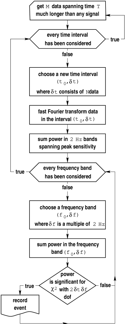
FIG. 1.: A flow chart for the short FFT algorithm for the power filter.

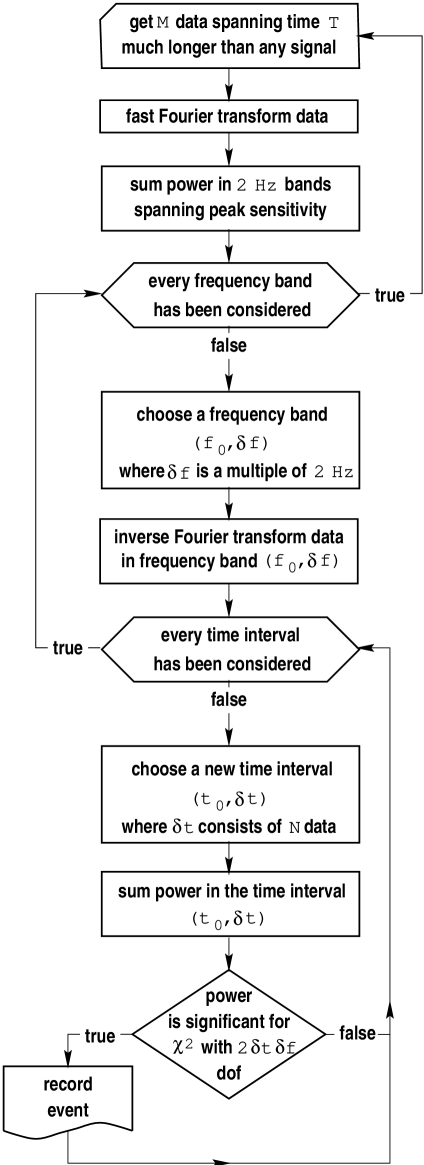
FIG. 2.: A flow chart for the long FFT algorithm for the power filter.

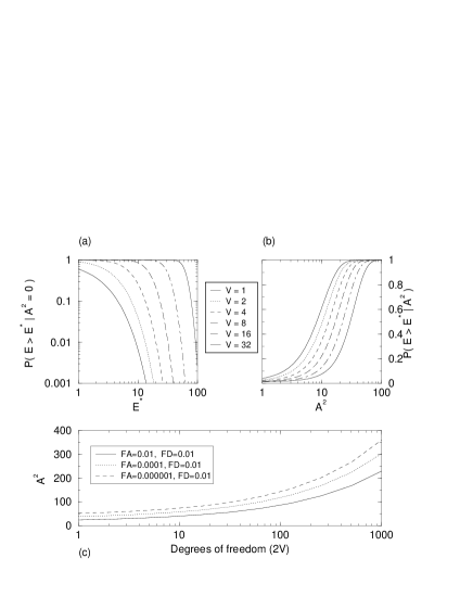
FIG. 3.: Cumulative probability functions for (a) the $\chi^{2}$ distribution and (b) the non-central $\chi^{2}$ distribution for various degrees of freedom $2V$. The curves in (a) give the probability that the power $\mathcal{E}$ exceeds a threshold ${\mathcal{E}}^{\star}$ when no signal is present. They can be used to fix the threshold given the time-frequency volume $V$ and the desired false alarm probability. The curves in (b) give the probability of detecting a signal whose power is $A^{2}$ in the time-frequency volume $V$ and given a threshold ${\mathcal{E}}^{\star}$, where the threshold ${\cal E}^{\star}$ is chosen to give a false alarm probability of 0.01. (c) The signal-to-noise ratio $A^{2}$ necessary to achieve a given false alarm probability (FA) and a false dismissal probability (FD) of 0.01 for various values of the number $2V$ of degrees of freedom.

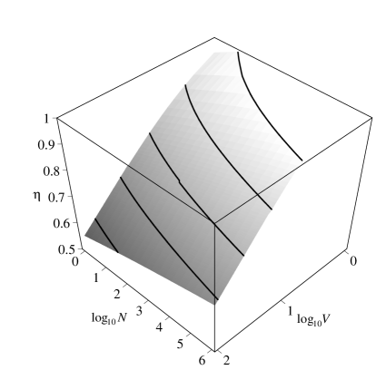
FIG. 4.: The relative effectiveness $\eta$ of the excess power method with respect to matched filtering, for the case where the time-frequency window is known in advance, as a function of the effective number of independent templates ${\cal N}_{\text{eff}}$ characterizing the space of signals being sought, and the time-frequency volume $V$. A false alarm probability corresponding to one false alarm per one hundred days of observation (taken to have $1.728\times 10^{9}$ independent arrival times), and a correct detection probability of $0.99$ were assumed. The quantity $\eta$ is the ratio of the minimum signal amplitude that is required to achieve these false alarm and dismissal probabilities for the excess power method, to the corresponding minimum amplitude for the matched filtering method. The loss in event rate due employing the excess power method rather than matched filtering is $\eta^{3}$. This plot can be generated by combining Eqs. (34), (40), (41) and (42) of the text.

FIG. 5.: The probability $P({\mathcal{E}}>{\mathcal{E}}^{\star}|0)$ of obtaining a value of ${\mathcal{E}}$ greater than a given threshold ${\mathcal{E}}^{\star}$, for stationary Gaussian noise in the absence of a signal, as a function of ${\mathcal{E}}^{\star}$. The quantity ${\mathcal{E}}$ has a $\chi^{2}$ distribution with $2V$ degrees of freedom, where $V$ is the time-frequency volume (14) of the signal being sought. The lines show theoretical curves generated according to the standard $\chi^{2}$ formula (24). The data points represent values obtained from Monte Carlo simulations (described in Sec. IV A), where the noise is Gaussian and white (circles) or colored (triangles).

FIG. 6.: The probability $P({\mathcal{E}}>{\mathcal{E}}^{\star}|A)$ of obtaining a value of ${\mathcal{E}}$ greater than or equal to a given threshold ${\mathcal{E}}^{\star}$ given the presence of a signal of power $A^{2}$ and stationary Gaussian noise, for several different values of the number $2V$ of degrees of freedom, as a function of $A^{2}$. For each $V$, the value of ${\mathcal{E}}^{\star}$ which gives a false alarm probability of $Q_{0}=0.01$ is used. The lines show theoretical curves generated according to the standard non-central $\chi^{2}$ formula (33). The data points represent values obtained from Monte Carlo simulations [described in Sec. IV A], where the noise is white (circles) or colored (triangles).

REFERENCES

- [1] A. Abramovici et al., Science 256, 325 (1992).
- [2] C. Bradaschia et al., Nucl. Inst. A. 289, 518 (1990).
- [3] B. Caron et al., Class. Quantum Grav. 14, 1461 (1997).
- [4] E. E. Flanagan and S. A. Hughes, Phys. Rev. D 57, 4535 (1998).
- [5] E. J. M. Colbert and R. F. Mushotzky, Astrophys. J. 519, 89 (1999).
- [6] A. Ptak and R. Griffiths, Astrophys. J. 517, L85 (1999).
- [7] S. F. Portgeis Zwart and S. L. W. McMillan, Astrophys. J. 528, L17 (2000).
- [8] K. S. Thorne, in 300 Years of Gravitation, ed. S. W. Hawking and W. Israel (Cambridge University Press, Cambridge, 1987), pp. 330-458.
- [9] B. Allen et al., GRASP: a Data Analysis Package for Gravitational Wave Detection, version 1.8.6. Manual and package at http://www.lsc-group.phys.uwm.edu.
- [10] N. Arnaud, F. Cavalier, M. Davier, and P. Hello, Phys. Rev. D 59, 082002 (1999).
- [11] See Time-Frequency Signal Analysis, edited by B. Boashash (John Wiley & Sons, Inc., New York, 1992) and references therein.
- [12] M. Feo, V. Pierro, I. M. Pinto and M. Ricciardi, in The Seventh Marcel Grossmann Meeting: Proceedings of the Meeting held at Stanford University, 24-30 July 1994, Part B, edited by R. T. Jantzen and G. M. Keiser (World Scientific Publishing Co., Singapore, 1994), pp. 1086–1089.
- [13] M. Feo, V. Pierro, I. M. Pinto and M. Ricciardi, in Gravitational Wave Detection (Proceedings of TAMA Workshop, Saitama, Japan), edited by K. Tsubono, M.-K. Fujimoto, K. Kuroda, (Universal Academy Press, Tokyo, Japan, 1997, pp. 329–330.
- [14] M. Feo, V. Pierro, I. M. Pinto and M. Ricciardi, in Edoardo Amaldi Foundation Series Volume 2. Proceedings of the International Conference on Gravitational Waves Sources and Detectors, March 19-23, 1996, Cascina (Pisa), Italy, edited by I. Ciufolini and F. Fidecaro, (World Scientific Publishing Co., Singapore, 1997), pp. 291–293.
- [15] A. Królak and P. Trzaskoma, Class. Quantum Grav. 13, 813 (1996).
- [16] J.-M. Innocent and B. Torrésani, in Mathematics of Gravitation, edited by A. Królak (Banach Center Publications, Warsaw, 1997).
- [17] P. Gonçalvès, P. Flandrin, and E. Chassande-Mottin, in Second Workshop on Gravitational Wave Data Analysis, edited by M. Davier and P. Hello (Éditions Frotières, Gif Sur Yvette, France, 1998), pp. 35–46.
- [18] E. Chassande-Mottin and P. Flandrin, ibid. pp. 47–52.
- [19] J.-M. Innocent and B. Torrésani, ibid. pp 53–64.
- [20] W. G. Anderson and R. Balasubramanian, Phys. Rev. D 60, 102001 (1999).
- [21] S. D. Mohanty, “A Robust Test for Detecting Non-Stationarity in Data from Gravitational Wave Detectors”, gr-qc/9910027.
- [22] B. F. Schutz, in The Detection of Gravitational Waves, edited by D. G. Blair,(Cambridge University Press, Cambridge, England, 1991), pp. 406–452.
- [23] N. Arnaud, F. Cavalier, M. Davier, P. Hello, and T. Pradier, gr-qc/9903025.
- [24] J. Fawcett and B. Maranda, IEEE Trans. Inform. Theory 37, 209 (1991).
- [25] R. L. Streit and P. K. Willett, IEEE Trans. Signal Processing 47, 1823 (1999).
- [26] J. Sylvestre, in preparation.
- [27] M. Abramowitz and I. A. Stegun, Handbook of Mathematical Functions (Dover, New York, 1972).
- [28] E. J. Groth, Ap. J., Suppl. Ser. 29, 285 (1975).
- [29] B. J. Owen, Phys. Rev. D 53, 6749 (1996).
- [30] E. E. Flanagan and S. A. Hughes, Phys. Rev. D 57, 4566 (1998).
- [31] L. A. Wainstein and V. D. Zubakov, Extraction of signals from noise (Prentice-Hall, London, 1962).
- [32] L. S. Finn, Phys. Rev. 46, 5236 (1992).
- [33] L. S. Finn and D. F. Chernoff, Phys. Rev. D 47, 2198 (1993).
- [34] S. A. Kassam, Signal Detection in Non-Gaussian Noise (Springer-Verlag, New York, 1988).
- [35] D. Lindley, Biometrika 44, 187 (1957).
- [36] G. Shafer, Journal of the American Statistical Association 77, 325 (1982).
- [37] L. S. Finn, Issues in Gravitational-Wave Data Analysis, 1997, submitted to the Proceedings of the Second Eduoardo Amaldi Conference, 1–4 July 1997.
- [38] J. D. E. Creighton, Phys. Rev. D 60, 022001 (1999).
- [39] J. D. E. Creighton, Phys. Rev. D 60, 021101 (1999).
- [40] S. V. Dhurandhar and M. Tinto, Mon. Not. R. Astron. Soc. 234, 663 (1988).
- [41] We can neglect here correction factors of the number of statistically independent time-frequency windows and source directions (see Sec. III B above) since we are not interested in the absolute value of , but rather merely in the functional dependence of on the data .
- [42] C. M. Will and A. G. Wiseman, Phys. Rev. D 54, 4183 (1996).
- [43] L. Blanchet, B. R. Iyer, C. M. Will, and A. G. Wiseman, Class. Quantum Grav. 13, 575 (1996).
- [44] W. Althouse, L. Jones, and A. Lazzerini, “Determination of global and local coordinate axes for the ligo sites,” Technical Report No. LIGO-T980044-08, unpublished (1998).
- [45] Position (elevation , latitude , and longitude using the WGS-84 ellipsoid earth model [44]) and orientations and of the and arms for various interferometers: VIRGO: [B. Mours (private communication)]; GEO-600: [http://www.geo600.uni-hannover.de/geo600/project/location.html]; TAMA-300: [M.-K. Fujimoto (private communication)].
- [46] B. Allen, “Gravitational wave detector sites,” unpublished (1996) gr-qc/9607075.