A new approach to electromagnetic wave tails on a curved spacetime

Abstract

We present an alternative method for constructing the exact and approximate solutions of electromagnetic wave equations whose source terms are arbitrary order multipoles on a curved spacetime. The developed method is based on the higher-order Green’s functions for wave equations which are defined as distributions that satisfy wave equations with the corresponding order covariant derivatives of the Dirac delta function as the source terms. The constructed solution is applied to the study of various geometric effects on the generation and propagation of electromagnetic wave tails to first order in the Riemann tensor. Generally the received radiation tail occurs after a time delay which represents geometrical backscattering by the central gravitational source. It is shown that for an arbitrary weak gravitational field it is valid that the truly nonlocal wave-propagation correction (the tail term) has a universal form which is independent of multipole structure of the gravitational source. In a particular case when the electromagnetic radiation pulse is generated by the wave source during a finite time interval, the structure of the wave tail at the time after the direct pulse has passed the gravitational source is in the first approximation independent of the higher multipole moments of the source of gravitation, including the angular momentum. These results are then applied to a compact binary system. It follows that under certain conditions the tail energy can be a noticeable fraction of the primary pulse energy, namely, it is shown that for a particular model the energy carried away by the tail can amount to $10\%$ of the energy of the low-frequency modes of the direct pulse. The present results indicate that the wave tails should be carefully considered in energy calculations of such systems and that the delay effect of the wave tails may be of great importance for their observational detection.

I Introduction

The problem of radiation propagation on a curved spacetime has been studied since the birth of general relativity, both as a matter of principle and as a basis of observational predictions. A field satisfying a hyperbolic differential equation (wave equation) propagates not only on the characteristic surfaces (light-cones), but also inside the light-cone in the form of wave tails which violate the Huygens’ principle [1, 2]. Physically speaking, the wave tails arise because the radiation is backscattered by the spacetime curvature. In certain cases backscattering can influence observations as it weakens and disperses sharp initial pulses. For instance, the electromagnetic (or gravitational) radiation from a pulsed source in the vicinity of a massive body reaching an asymptotic observer is received as two distinct pulses: one arriving along the direct route and the other, the tail, effectively being scattered off by the central body [3, 4, 5].

Recently the wave tails have become to be recognized as factors in the planned observational detection of the gravitational waves by forthcoming laser interferometric detectors [6, 7, 8, 9, 10, 11]. It has also been shown that the wave tails play an important role in the generation of gravitational waves by the orbital inspiral of a compact binary system [12, 13, 14]. The close relationship between the generation of the wave tails and gravitational focusing has been demonstrated in Ref. [15].

The process of wave propagation on a curved spacetime being quite complicated, usually the wave equation is solved in the weak-field and slow-motion limit by the method of successive approximations, using multipole expansion in one way or another (see e.g. [16, 17, 18, 19]). A general solution of the electromagnetic wave equation in a curved space was constructed by DeWitt and Brehme [20] in terms of the Green’s function, using the Hadamard procedure [1]. The general solution demonstrates scattering of the electromagnetic radiation by the spacetime curvature. An alternative technique for investigating electromagnetic radiation in the Schwarzschild and Kerr metrics was worked out following the Regge-Wheeler approach to metric perturbations [21, 22, 23]. This technique relies on an expansion into generalized spherical harmonics and is especially useful when radiation emanates from a given multipole moment of the source. Herein, for a point charge an infinite sum emerges. The benefit, however, is that the obtained solution is also valid for the strong-field region.

We have recently developed a new method [24, 25, 26] for calculating the exact solutions of scalar and tensor wave equations whose source terms are arbitrary-order multipoles on a curved spacetime. The developed method is based on the higher-order fundamental solutions (Green’s functions) for wave equations which are defined in our paper [27] as the distributions that satisfy wave equations with the corresponding order covariant derivatives of the Dirac delta function as the source terms. Provided that the classical Green’s function and the multipole expansion of the source term are given, there is no need for a small expansion parameter within the framework of our formalism and in certain cases we can even find the exact multipole solutions for a strong field. Our approach also enables us to find an approximate solution provided that an approximate form of the classical Green’s function is known which is the case for most spacetimes. Moreover, it proves to be more advantageous to apply our algorithm [25, 26], instead of the traditional approach of successive approximations, as the amount of computations involved is considerably reduced and, as will be demonstrated below, some features unrevealed by the successive approximation methods are brought forward. It is worthwhile to point out that, as distinct from most of papers dedicated to the topics of wave tails in which the source of the gravitational field is regarded as a point mass, within the framework of our approach [24, 25] the extension of the source of gravitation is finite. The last circumstance enables us to avoid in computations the additional non-physical singularity, the regularizing of which may bring on difficulties in interpreting the results.

On the basis of our method [25] of higher-order Green’s functions we have developed a new approach to the electromagnetic radiation on a curved spacetime. In a recent communication [28] we presented some initial results obtained within the framework of this approach. Namely, we considered a pulsed source of electromagnetic radiation in arbitrary bounded motion in a weak gravitational field and concluded that generally the received radiation tail arrives after a time delay which represents geometrical backscattering by the central gravitational source. This delay effect of the wave tails may be of great importance by their observational detection. Further, by applying this approach to a compact astrophysical binary system we demonstrated that under certain conditions the tail energy can be a noticeable fraction of the direct pulse energy. The underlying formulas involved are herein published for the first time.

The wider aim of the present paper is to provide a comprehensive view of our new approach to the electromagnetic radiation, more fully describe the already published results and expand upon them. Specifically, among the rest we will prove the following. (i) Vanishing of the Ricci curvature tensor is the necessary and sufficient condition for the validity of the Huygens’ principle in the first-order approximation, as it is already known. (ii) If the direct pulse of electromagnetic radiation has passed the gravitational source, then in the first approximation the structure of electromagnetic wave tails is independent of the higher multipole moments of the gravitational source, including the angular momentum. (iii) In an arbitrary weak gravitational field it is valid that in the first approximation the nonlocal radiative electromagnetic tail term at infinity acquires a universal form, viz. Eq. (63), which is independent of the multipole order. (The limitations of applicability as well as the relationships of these results with the earlier ones will be discussed in due course below.)

Finally, we think that our method deserves to be presented in detail as it may prove to be useful also for the theoretical investigations of detection of gravitational waves performed within the framework of the LISA mission.

The remainder of the paper is organized as follows. Sec. II gives a review of the theory of classical and higher-order Green’s functions (fundamental solutions) for vector wave equations, as well as the recurrent formulas for calculating the Green’s functions proceeding from the Hadamard coefficients. In Sec. III we determine the multipole moments of electromagnetic field source term with respect to a given worldline, and also present an algorithm for calculating the exact multipole solutions of the wave equations. In Sec. IV the main results are obtained. We consider the tail term of the retarded Green’s function expanded to first order in the gravitational potential, and give the first-order tail term for the multipole solutions of electromagnetic field (IV A, B). In Sec. IV D we turn to nonlocal radiative wave-propagation correction in the far wave zone. We estimate the magnitude of electromagnetic radiation energy and find that,compared to the energy of the direct pulse, the value of tail energy can be considerable and may thus have astrophysical significance. Limitations to the applicability of the derived conclusions are also considered. Sec. V contains brief concluding remarks. Appendix explains our notation and displays the relevant definitions.

II METHOD OF HIGHER-ORDER GREEN’S FUNCTIONS

To investigate the electromagnetic wave tails within the framework of general relativity, we first consider on a pseudo-Riemannian 4-space $M$ a vector wave equation

$${\hbox{{\bf L u =f}}},$$ (1)

which in local coordinates can be written in the following coordinate invariant form (for our notation see Appendix)

$$Lu_{c}:=g^{ab}\nabla_{a}\nabla_{b}u_{c}-R^{a}_{c}u_{a}=f_{c},$$ (2)

where the contravariant components of the metric tensor $g^{ab}$ are assumed to be of differentiability class $C^{\infty}$, and $R_{ac}$ are the covariant components of the Ricci tensor. The inhomogeneous term $\bf f$ of Eq. (1) is in general a distribution, i.e. ${\bf f}\in{\cal D}^{\prime 1}(\Omega)$. In order to be able to complete the construction of ${\bf u}$, we restrict the solutions to a causal domain $\Omega\subseteq M$ (see point 5 in Appendix and Refs. [2, 29]).

The notation and basic definitions used in this paper will be in detail presented in Appendix. Here we touch on only the spacetime subdomains frequently resorted to. $C^{+}(y)$ is the future light cone, i.e. the set of all points $x\in\Omega$ that can be reached along future-directed null geodesics from $y$; $C^{-}(y)$ is the past light cone, defined similarly by past-directed geodesics. The sets $D^{\pm}(y)$ denote the respective interiors of the future and past light cones $C^{\pm}(y)$, whereas $J^{\pm}(y):=D^{\pm}(y)\cup C^{\pm}(y)$.

A Classical (zeroth-order) Green’s function

The classical (i.e. zeroth-order) Green’s function, or fundamental solution as mathematicians would say, ${\bf G}(x,y)$ of the wave equation (1) satisfies

$${\bf LG}(x,y)={\bf g}(x,y)\delta(x,y),$$ (3)

where $\delta(x,y)$ is the Dirac delta distribution, with $(\delta(x,y),\phi(x)):=\phi(y)$ for all $\phi\in C_{0}^{\infty}(\Omega)$ and ${\bf g}(x,y)$ is a transport bivector (for its defining equations see Appendix).

As in the case of flat spacetime, there are two particularly important Green’s functions of the wave equation (1): the retarded Green’s function ${\bf G}^{+}(x,y)$ and the advanced Green’s function ${\bf G}^{-}(x,y)$. It has been demonstrated that they have the following form [2, 29]:

$${\bf G}^{\pm}(x,y)={1\over 2\pi}\left[{\bf U}(x,y)\delta_{\pm}^{(0)}(\sigma(x,y))+{\bf V}(x,y)\Theta_{\pm}(\sigma(x,y))\right],$$ (4)

where the bitensors ${\bf U}\in C^{\infty}(\Omega\times\Omega)$ and ${\bf V}\in C^{\infty}(\Omega\times\Omega)$ are the Hadamard coefficients of the classical Green’s functions (4) of the vector wave equation (1).

The bitensor ${\bf U}$ in Eq. (4) is determined by the following transport equation and normalization condition:

$$\sigma^{;a}(x,y)\nabla_{a}U^{i}_{b}(x,y)+M(x,y)U^{i}_{b}(x,y)=0,$$ (5)

$$U^{i}_{a}(x,x)=\delta^{i}_{a},$$ (6)

where

$$M(x,y):={1\over 2}\nabla^{a}\nabla_{a}\sigma(x,y)-4.$$ (7)

It is well known that the bivector ${\bf U}$ can be written as [29, 20]

$${\bf U}:={\bf g}(x,y)k(x,y),$$ (8)

where ${\bf g}(x,y)$ and $k(x,y)$ are respectively the transport bivector and scalarized van Vleck determinant, defined in Appendix.

The bivector ${\bf V}\in C^{\infty}(\Omega\times\Omega)$ in Eq. (4), called the tail term, is determined by the characteristic Cauchy problem. It corresponds to the ’logarithmic term’ of the Hadamard construction and is inherently connected with the concept and validity of Huygens’ principle [1]. In the regions $D^{\pm}(y)$ the vector field ${\bf V}$ satisfies the homogeneous wave equation

$${\bf LV}(x,y)=0,$$ (9)

which is completed by the characteristic initial conditions

$$\sigma^{;a}(x,y)\nabla_{a}V^{i}_{b}(x,y)+(M(x,y)+2)V^{i}_{b}(x,y)=-{1\over 2}LU^{i}_{b}(x,y),$$ (10)

for $\forall x\in C^{\pm}(y)$.

Sometimes, instead of solving the differential equations (9) and (10) straightforwardly, in order to find the tail term ${\bf V}$, it is preferable to use an exact integral equation. We proceed from the fact that Friedlander has derived the corresponding exact integral equation for the tail term of the Green’s function of the scalar wave equation (Eq. (5.4.19) in Ref. [29]), and suggested a procedure for obtaining the tensor field Green’s functions from the scalar Green’s function. Thus, generalizing the above-mentioned Friedlander’s equation, we find for the vector case when $x\in D^{+}(y)$, the tail term ${\bf V}$ satisfies the following exact integral equation:

$$V_{a}^{i}(x,y)+{1\over 2\pi}\int_{\Sigma(y)}V^{p}_{a}(x,z)LU^{i}_{p}(z,y)\mu_{\sigma(z,y)}(z)+{1\over 2\pi}\int_{S(y)}U^{p}_{a}(x,z)LU^{i}_{p}(z,y)\omega(z)=0,$$ (11)

Here: the $3$-surface $\Sigma(y)$ and the $2$-surface $S(y)$ are defined by $\Sigma(y):=C^{+}(y)\cap J^{-}(x)$ and $S(y):=C^{+}(y)\cap C^{-}(x)$, respectively; the operator ${\bf L}$ acts at $z$; the $3$-form $\mu_{\sigma(z,y)}$ and the $2$-form $\omega$ are defined in Appendix by Eqs. (78) and (80).

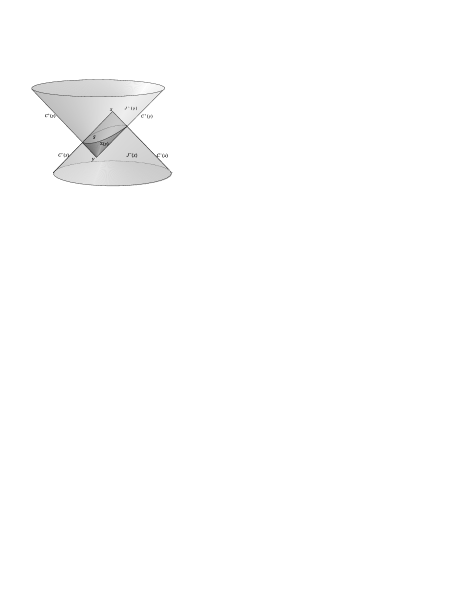
FIG. 1.: The geometric regions occurring in Eq. (9): an illustration on a 3-dimensional intersection of the Minkowski space with the plane $x^{3}={\text{c}onst}$. The darker region on the future light cone $C^{+}(y)$ is the hypersurface $\Sigma(y)$ whose $2$-dimensional boundary $S$ is represented by an ellipse which is the intersection of the light cones $C^{+}(y)$ and $C^{-}(x)$.

We will use Eq. (11) in Sec. IV for obtaining an expression for electromagnetic wave tails in the first-order approximation.

Only the retarded Green’s functions ${\bf G}^{+}$ will be discussed, as the corresponding results for the advanced Green’s functions ${\bf G}^{-}$ can be obtained by reversing the time orientation on the domain $\Omega$.

B Higher-order Green’s functions for vector wave equations

Let $\Omega$ be a causal domain. Then the tensor differential operator ${\bf L}$ in (1) has a unique retarded $\mu$th-order Green’s function ${\bf G}^{+}$ on $\Omega$ such that

$\displaystyle LG^{+a}_{iJ(\mu)}(x,y)=(-1)^{\mu}\nabla_{B(\mu)}\left[g^{a}_{i}(x,y)g^{B(\mu)}_{J(\mu)}(x,y)\delta(x,y)\right],$

$\displaystyle\text{supp}~{}{\bf G}^{+}\subset J^{+}(y).$If test vector fields ${\bf\Phi}\in{\cal D}^{1}(\Omega)$ are such that $\text{supp}~{}{\bf\Phi}\subset\Omega\backslash\{y\}$, then the retarded $\mu$th-order Green’s function ${\bf G}^{+}$ is of the following form:

$${\bf G}^{+}={1\over 2\pi}\left[\sum\limits_{\nu=0}^{\mu}{\bf W}_{\nu}^{\mu}\delta_{+}^{(\mu-\nu)}(\sigma)+{\bf W}_{\mu+1}^{\mu}\Theta_{+}(\sigma)\right],$$ (12)

where ${\bf W}_{\nu}^{\mu},\nu=0,\dots\mu+1$ are bitensor fields of rank $1$ at $x$ and of rank $\mu+1$ at $y$ recursively determined by

$$W^{\mu~{}a}_{\nu~{}i~{}J(\mu)}=\sigma_{;j_{\mu}}W^{\mu-1~{}a}_{\nu~{}i~{}J(\mu-1)}+W^{\mu-1~{}a}_{\nu-1~{}i~{}J(\mu-1);j_{\mu}},$$ (13)

$${\bf W}^{\mu}_{-1}={\bf W}^{\mu}_{\mu+2}:=0,\;\quad{\bf W}^{0}_{0}:={\bf U},\;\quad{\bf W}^{0}_{1}:={\bf V},$$ (14)

where $\nu=0,\dots,\mu+1$.

This statement was first proposed by us without proof in [27], its proof can be found in [24]. Eqs. (14) provide a simple recurrent algorithm for calculating the $\mu$th-order Green’s functions for the vector wave equation (1) proceeding from the Hadamard coefficients ${\bf U}$ and ${\bf V}$ of classical Green’s function (4). The formulas (12-14) constitute the main mathematical tool which allows construction of our exact multipole solutions of vector wave equations.

III EXACT SOLUTIONS

A Multipole expansion of the electromagnetic field source

On the basis of Dixon’s ideas [30] we will now construct a multipole expansion of the electromagnetic field source ${\bf f}$ as follows. We first choose a unique timelike worldline $\xi$ lying inside the worldtube $\Gamma\subset\Omega$ of the source of the electromagnetic field that represents its dynamical properties. Such a curve can be given as a $C^{\infty}$ embedding $t\to y(t)\in\xi$ of an open interval $I\subset{\cal R}$ into $\Omega$, where ${\cal R}$ is the real line. We set $v^{i}(t)={dy^{i}\over dt}$; this vector is assumed to be timelike and future-directed, and it is convenient to normalize the parametrization so that $t$ is the proper time, which means that $v^{i}v_{i}=1$. For $y(t)\in\xi$ we define $\Sigma(t):=\{x|v^{i}(t)\sigma_{;i}(x,y(t))=0\}$, the spacelike hypersurface consisting of all geodesics through $y(t)$ orthogonal to ${\bf v}(t)$. We suppose that there exists a $3$-form $\mu_{\Sigma}$ such that $\mu(x)=d\eta\wedge\mu_{\Sigma}$ on $\text{supp}~{}{\bf f}$; here $\eta(x)$ is defined by $v^{i}(\eta(x))\sigma_{;i}(x,y(\eta(x)))=0$, $y(\eta)\in\xi$. For the sake of simplicity, we assume also that $\text{supp}~{}{\bf f}$ is compact in the domain $\Omega$. Regarding the source function ${\bf f}$ as a regular distribution with compact support, we can write

$\displaystyle({\bf f},{\bf\Phi})=\int_{I}dt\int_{\Sigma(t)}<{\bf f}(x){\bf\Phi}(x)>\mu_{\Sigma}(x),$where $<{\bf f\Phi}>$ denotes the scalar product. Let ${\bf\bar{M}}_{\mu}(t)$ be $C^{\infty}$ tensor fields of corresponding ranks $\mu+1\geq 1$ at $y(t)\in\xi$, with $\text{supp}~{}{\bf\bar{M}}_{\mu}(t)$ compact, and let $N\geq 0$ be a integer. We consider the line distributions

$$f^{a}_{N}=\sum\limits_{\mu=0}^{N}(-1)^{\mu}\bar{M}_{\mu}^{I(\mu)j}(t)\nabla_{A(\mu)}g^{A(\mu)}_{I(\mu)}(x,y(t))g^{a}_{j}(x,y(t))\bar{\delta}(x,\xi)\in{\cal E}^{\prime 1}(\Omega)$$ (15)

which assigns to any ${\bf\Phi}\in C_{0}^{\infty}(\Omega)$ the number

$$({\bf f}_{N},{\bf\Phi}):=\sum\limits_{\mu=0}^{N}\int_{I}\bar{M}_{\mu}^{I(\mu)j}(t)\phi_{j;I(\mu)}(y(t))dt.$$ (16)

In the particular case of $N=0$ the formula (16) means that

$\displaystyle(g^{a}_{i}(x,y(t))\bar{M}^{i}_{0}(t)\bar{\delta}(x,\xi),\phi_{a}(x)):=\int_{I}\bar{M}_{0}^{i}(t)\phi_{i}(y(t))dt.$

Let us now choose a test function so that $\text{supp}~{}{\bf\Phi}\supset\text{supp}~{}{\bf f}$. If for all test functions such that $\text{supp}~{}{\bf\Phi}\supset\text{supp}~{}{\bf f}$, the following equation is valid

$$({\bf f}_{N},{\bf\Phi})=\int_{I}dt\int_{\Sigma(t)}<{\bf f}(x){\bf\Phi}_{N}(x,t)>\mu_{\Sigma}(x),$$ (17)

where ${\bf\Phi}_{N}$ is determined by the Taylor expansion of the vectorfunction ${\bf\Phi}$

$\displaystyle\phi^{a}_{N}(x,t):=\sum\limits_{\mu=0}^{N}{(-\mu)^{l}\over 2^{\mu}\mu!}g^{aj}(x,y(t))\sigma^{;i_{1}}(x,y(t))\dots\sigma^{;i_{\mu}}(x,y(t))\phi_{j;I(\mu)}(y(t)),$then the line distribution ${\bf f}_{N}$ is called the $N$th-order multipole expansion of the source function ${\bf f}$.

If ${\bf f}_{N}$ is the $N$th-order multipole expansion of ${\bf f}$, then it follows form (16) and (17) that one can choose

$$\bar{M}_{\mu}^{I(\mu)j}(t)={(-1)^{\mu}\over 2^{\mu}\mu!}\int_{\Sigma(t)}g^{j}_{a}(x,y(t))f^{a}(x)\sigma^{;i_{1}}(x,y(t))\dots\sigma^{;i_{\mu}}(x,y(t))\mu_{\Sigma}(x).$$ (18)

The tensor field ${\bf\bar{M}}_{\mu}(t)$ determined by the expression (18) is called the $2^{\mu}$-pole moment of the field source ${\bf f}$ with respect to $\xi$. One should mention that Eqs. (16) and (17) do not uniquely determine the structure of the multipole moments ${\bf\bar{M}}_{\mu}$ in Eq. (18). For example, let us define a set of new multipole moments ${\bf M}_{\mu}(t)$ by relations $M_{\mu}^{I(\mu)j}(t)=\bar{M}_{\mu}^{I(\mu)j}(t)+D_{\mu-1}^{I(\mu-1)j}v^{i_{\mu}}+{\delta\over\delta t}D_{\mu}^{I(\mu)j}(t)\;$, $\mu\leq N\;$, $D_{N}^{I(N)j}=0\;$, where the symbol ${\delta\over\delta t}$ denotes the absolute derivative along the worldline $\xi$. Now, integrating Eq. (16) by parts, it follows that ${\bf f}_{N}$ remains unchanged for arbitrary tensor fields ${\bf D}_{\mu}(t)$ with compact support.

The multipole moments defined by Eq. (18) are obviously symmetric in the first $\mu$ indices, i.e. $\bar{M}_{\mu}^{i_{1}\dots i_{\mu}j}=\bar{M}_{\mu}^{(i_{1}\dots i_{\mu})j}$. They also satisfy the orthogonality condition $\bar{M}_{\mu}^{i_{1}\dots i_{\mu}j}v_{i_{\mu}}=0$. One should say, though, that due to charge conservation, $\nabla_{a}f^{a}=0$, the multipole moments of different orders ${\bf\bar{M}}_{\mu}$ are interrelated through differential constraints. For that reason their direct usage in solving particular physical problems is inconvenient. However, Dixon demonstrated in Ref. [30] that by means of the multipole moments ${\bf\bar{M}}_{\mu}$ a new set of reduced multipole moments ${\bf Q}_{\mu}\;$, $\mu\geq 1$ can be constructed, which together with the total charge $Q$ will completely describe the four-current ${\bf f}$. If $Q=\text{const}$, then the charge is automatically conserved, and thus the multipole moments of different orders ${\bf Q}_{\mu}\;$, $\mu\geq 1$ are independent. Dixon’s reduced multipole moments have the following symmetry and orthogonality properties:

$$Q_{\mu+1}^{i_{1}\dots i_{\mu}jk}=Q_{\mu+1}^{(i_{1}\dots i_{\mu})[jk]}\quad\text{for}\quad\mu\geq 0,$$ (19)

$$Q_{\mu+1}^{i_{1}\dots i_{\mu-1}[i_{\mu}jk]}=0,\quad Q_{\mu+1}^{i_{1}\dots i_{\mu}jk}v_{i_{\mu}}=0\quad\text{for}\quad\mu\geq 1.$$ (20)

Following Dixon’s work [30], we will in this paper approximate the source of electromagnetic waves ${\bf f}$ by its $N$th-order multipole expansion (15) replacing, however, the multipole moments ${\bf\bar{M}}_{\mu}(t)$ with the reduced ones ${\bf M}_{\mu}(t)$:

$$M_{\mu}^{I(\mu)j}:={2\mu\over\mu+1}Q^{i_{1}i_{2}\dots i_{\mu-1}i_{1}j},\qquad\mu\geq 1.$$ (21)

B Exact solutions of vector wave equations with a multipole source term

In one of our earlier papers [25] we demonstrated how to obtain a solution by way of describing $2^{\mu}$-pole radiation of a vector field in terms of the higher-order Green’s functions, i.e. how to calculate the retarded solution ${\bf u}^{+}_{\mu}$ of the vector wave equation

$\displaystyle Lu^{a}_{\mu}=\rho^{a}_{\mu}$with a multipole source term

$$\rho^{a}_{\mu}:=(-1)^{\mu}M_{\mu}^{I(\mu)j}(t)\nabla_{A(\mu)}(g^{A(\mu)}_{I(\mu)}(x,y(t))g^{a}_{j}(x,y(t))\bar{\delta}(x,\xi)).$$ (22)

Here ${\bf M}_{\mu}(t)$ is a tensor field of order $\mu+1$ on the worldline $\xi$ of the source of (electromagnetic) radiation and the coordinates of the points of the line $\xi$ are denoted by $y(t)$, where the parameter $t$ is the proper time along $\xi$. Let us suppose that there is a $t_{0}\in I$ such that ${\bf M}_{\mu}(t)=0$ for $t<t_{0}$. If ${\bf M}_{\mu}$ is determined by relations (21), it follows from the symmetry properties of Dixon’s moments(20) that $\nabla_{a}\rho^{a}_{\mu}=0$, i.e.

$$(\nabla_{a}\rho^{a}_{\mu},\phi)=-(\rho^{a}_{\mu},\nabla_{a}\phi)=0.$$ (23)

On the domain $J^{+}(\xi)\backslash\{\xi\}$, with $J^{+}(\xi):=\bigcup_{y\in\xi}J^{+}(y)$, the solution ${\bf u}^{+}_{\mu}$ can be represented as a regular distribution (function). To find a form of the solution suitable for applications it is reasonable to define a new, retarded time coordinate $\tau(x)$ as follows

$$\sigma(x,y(\tau(x)))=0,\qquad y(\tau)\in C^{-}(x).$$ (24)

Evidently, the future light cone $C^{+}(y(t))$ is determined by the equation $\tau(x)=t$. We denote the corresponding Leray form by $\mu_{\tau}(x)$, i.e. $d\tau\wedge\mu_{\tau}(x)=\mu(x)$ on $J^{+}(\xi)\backslash\{\xi\}$, (see Ref. [29]). On the surface $C^{+}(y(t))\backslash\{y(t)\}$ we have

$$d\sigma=-\sigma_{;i}(x,y(t))v^{i}(t)|_{\tau(x)=t}d\tau.$$ (25)

In what follows we shall use the notation

$$\psi(x,t):=-\sigma_{;i}(x,y(t))v^{i}(t).$$ (26)

Due to the theorem 5 proved in [25], the unique retarded solution ${\bf u}^{+}_{\mu}$ of Eq. (22) can be written in the following form:

$$u^{+a}_{\mu}(x)={1\over 2\pi}\sum\limits_{\nu=0}^{\mu}\left[\left({1\over\psi(x,t)}{d\over dt}\right)^{\mu-\nu}{M_{\mu}^{I(\mu)j}(t)W^{\mu~{}a}_{\nu~{}j~{}I(\mu)}(x,y(t))\over\psi(x,t)}\right]_{t=\tau(x)}$$ (27)

$$+{1\over 2\pi}\int_{t_{0}}^{\tau(x)}V^{a}_{j;I(\mu)}(x,y(t))M_{\mu}^{I(\mu)j}(t)dt,\qquad\forall x\in J^{+}(\xi)\backslash\{\xi\},$$ (28)

where the quantities ${\bf W}_{\nu}^{\mu}$, $\nu=0,\dots,\mu$ are bitensor fields of rank $1$ at $x$ and of rank $\mu+1$ at $y$ recursively determined by Eqs. (14), and the bitensor field ${\bf V}$ is the tail term of the Green’s function of Eq. (1). Identifying the tensor field ${\bf M}_{\mu}$ in Eqs. (22) and (28) with the tensor field (21), defined via Dixon’s multipole moments, it is easy to see that due to Eq. (23), and the uniqueness of the retarded solution of the wave equation, the solution $u^{+a}_{\mu}$ satisfies the gauge condition $\nabla_{a}u^{+a}_{\mu}=0$. Consequently, the quantity $u^{+a}_{\mu}$ can be interpreted as the retarded potential of electromagnetic field. Thus Eq. (28) with the recurrence system (14) enables one to find with admirable ease the exact multipole solution of arbitrary order for the electromagnetic wave equation (22) by means of the world function $\sigma$, transport bitensor ${\bf g}$ and tail term ${\bf V}$ of the classical Green’s function (4).

IV ELECTROMAGNETIC WAVE TAILS IN CASE OF A WEAK GRAVITATIONAL FIELD

Application of formulas (28) presupposes knowledge of the tail term ${\bf V}$ of the classical Green’s function and the world function $\sigma$, the exact forms of which, however, have been thus far calculated for some particular cases only, such as for example the Bianchi-type I metric [31], de Sitter metric [29] and a class of Robertson-Walker metrics [32]. Nevertheless, for most cases approximate forms of ${\bf V}$ and $\sigma$ are known and can be used within the framework of our formalism in obtaining approximate solutions.

We assume that the gravitational field is weak and therefore use a perturbational approach. The metric tensor and other geometrical quantities are supposed to depend on a small parameter $\varepsilon$ which determines the order of deviation from flat spacetime. Such expansion has been used for instance for the electromagnetic field in Ref. [33] and for gravitational waves in Ref. [15].

A First-order tail term for the Green’s function

We assume that the metric tensor $g_{ab}$ is expanded up to the first order in $\varepsilon$, so that the zeroth-order term is the metric tensor of the flat spacetime $\!\!\!\!{\mathop{\;\;\;g_{ab}}\limits_{0}}$, i.e.

$$g_{ab}=\!\!\!\!{\mathop{\;\;\;g_{ab}}\limits_{0}}+\varepsilon\gamma_{ab}+O(\varepsilon^{2}),$$ (29)

$$g^{ab}=\!\!\!\!{\mathop{\;\;\;g^{ab}}\limits_{0}}-\varepsilon\gamma^{ab}+O(\varepsilon^{2})$$ (30)

with $\gamma^{ab}=\!\!\!\!{\mathop{\;\;\;g^{ac}}\limits_{0}}\!\!\!\!{\mathop{\;\;\;g^{bd}}\limits_{0}}{\gamma_{cd}}$. The world function $\sigma(x,y)$, the transport tensor ${\bf g}(x,y)$ and the scalarized van Vleck determinant $k(x,y)$ can then also be expanded in the parameter $\varepsilon$. We have

$$\sigma={\mathop{\sigma}\limits_{0}}+\varepsilon{\mathop{\sigma}\limits_{1}}+O(\varepsilon^{2}),$$ (31)

$${\bf g}={\mathop{\bf g}\limits_{0}}+\varepsilon{\mathop{\bf g}\limits_{1}}+O(\varepsilon^{2}),$$ (32)

$$k={\mathop{k}\limits_{0}}+\varepsilon{\mathop{k}\limits_{1}}+O(\varepsilon^{2}),$$ (33)

where $\mathop{\sigma}\limits_{0}$, ${\mathop{\bf g}\limits_{0}}$ and $\;\mathop{k}\limits_{0}=1$ are the corresponding quantities of flat spacetime. The expansions of the Ricci tensor and the tail term ${\bf V}$ of the classical Green’s function begin with terms which are small of the first order, that is

$$R_{ab}=\varepsilon\!\!\!\!\!{\mathop{\;\;\;R_{ab}}\limits_{1}}+O(\varepsilon^{2}),$$ (34)

$${\bf V}=\varepsilon{\mathop{\bf V}\limits_{1}}+O(\varepsilon^{2}).$$ (35)

Due to the tensor character of the expressions obtained, they can be used in all the coordinate systems, where the metric preserves the form (30). Up to now we have where necessary meticulously inserted the underscripts $0$ and $1$ denoting the zeroth-order terms (i.e. the flat spacetime quantities) and the first-order terms, respectively. The Ricci tensor $R_{ab}$ and the tail term ${\bf V}$ being small of the first order, we will omit these underscripts where confusion is excluded, and write the results in what follows to the first-order approximation.

Next we will find an explicit expression for the leading member of the expansion of the tail term ${\bf V}$ proceeding from the integral equation (11). Since ${\bf V}$ is small of the first order, it follows from Eq. (10) that the quantity $LU^{i}_{b}(x,y)$ is also small of the first order. Thus the first integral in Eq. (11) is a second order small quantity, whereas the first factor $U^{a}_{p}(x,z)$ under the second integral in Eq. (11) may be considered as a zeroth order quantity. Hence, taking into account Eq. (8) with $\;\mathop{k}\limits_{0}=1$, the vector integral equation (11) reduces to

$$V^{i}_{a}(x,y)=-{1\over 2\pi}\int_{S(y)}g^{p}_{a}(x,z)LU^{i}_{p}(z,y)\omega(z)+O(\varepsilon^{2}).$$ (36)

Likewise, the first factor under the last integral is of zeroth order, and if we would use Minkowskian coordinates in the flat spacetime we could write $g^{p}_{a}=\delta^{p}_{a}+O(\varepsilon)$. Nevertheless, in order to be able to use general curvilinear coordinates in the flat spacetime without any need for modifications in the integral in Eq. (36), we prefer to keep the more general expression $g^{p}_{a}(x,z)$. The same will be done in similar cases below.

To calculate the factor $LU^{i}_{a}$ under the last integral we need the linear terms in the expansions of $g^{i}_{a}(x,y)$ and $k(x,y)$ which can obtained as follows. Expanding the defining equation $\sigma^{;a}\nabla_{a}g^{a}_{i}(x,y)=0$ of the transport bivector, we have

$$g_{ai}(x,y)=\!\!\!\!{\mathop{\;\;\;g_{ai}}\limits_{0}}+{\varepsilon\over 2}\int_{0}^{1}\!\!\!{\mathop{\;\;g{{}^{p}_{a}}}\limits_{0}}(y,z(\lambda))\!\!{\mathop{\;\;g{{}^{q}_{i}}}\limits_{0}}(y,z(\lambda))\left[\gamma_{q(p;r)}(z(\lambda))-\gamma_{pr;q}(z(\lambda))\right]\dot{z}^{r}d\lambda+O(\varepsilon^{2}).$$ (37)

Here, as well as in the next integral, integration is performed along the geodesic $z(\lambda)$ connecting the points $x$ and $y$, where $\lambda$ is an affine parameter on the geodesic, such that $z(1)=x$, $z(0)=y$.

Next substituting Eq. (8) with Eq. (37) into Eq. (6) yields for the scalarized van Vleck determinant (82) the following first-order expression

$$k(x,y)=1+{1\over 8}\sigma^{;a}(x,y)\sigma^{;b}(x,y)\int_{0}^{1}\lambda(1-\lambda)g^{p}_{a}(x,z(\lambda))g^{q}_{b}(x,z(\lambda))R_{pq}(z(\lambda))d\lambda+O(\varepsilon^{2}).$$ (38)

Finally, after quite simple but voluminous calculations we obtain from Eqs. (36-38) the seeked expression for the first-order tail term

$$V^{i}_{a}(x,y)={1\over 4\pi}\left\{g^{i}_{a}\nabla_{b}\left[\sigma^{-1}(x,y)P^{b}(x,y)\right]+\sigma^{-1}(x,y)F^{i}_{a}(x,y)\right\},$$ (39)

where

$$P^{b}(x,y):=\int_{\Sigma(y)}g^{b}_{p}(x,z)G^{pq}(z)d\Sigma_{q}(z),\\$$ (40)

$$F^{i}_{a}(x,y):=\int_{S(y)}g^{p}_{a}g^{iq}\left(4R_{[p}^{r}D_{q]r}+RD_{pq}+2R_{pq}\sigma(x,y)\right)\omega(z).$$ (41)

Here $G^{pq}:=R^{pq}-{1\over 2}g^{pq}R$ are the contravariant components of Einstein’s tensor, $R$ is the Ricci scalar, $D_{pq}:=\sigma_{;[p}(z,x)\sigma_{;q]}(z,y)$ and $d\Sigma_{q}(z)$ denotes the $3$-surface element on $\Sigma(y)$ defined by

$$d\Sigma_{p}(z)={1\over 6}\sqrt{g(z)}\epsilon_{pqrs}dz^{q}\wedge dz^{r}\wedge dz^{s},$$ (42)

where $\epsilon_{pqrs}$ are the components of the discriminant tensor with $\epsilon_{0123}=1$.

It can be shown that $V^{i}_{a}(x,y)$ remains bounded when $x\to\bar{x}\in C^{+}(y)$. From Eqs. (39-41) we see that $V^{i}_{a}$ vanishes for every $x\in\Omega$ and $y\in\Omega$ if $R_{pq}(z)=0$, $\forall z\in\Omega$. It is the necessary and sufficient condition for validity of Huygens’s principle in the first-order approximation [33, 34].

Among the astrophysical applications of great interest is the case in which the source of gravitation is spatially isolated, i.e. $\text{supp}~{}R_{ab}\subset\tilde{\Gamma}$, where $\tilde{\Gamma}$ is the world tube of the gravitational field source. In this case it is reasonable to divide the spacetime domain $J^{+}(y)$ into the following three subdomains:

$\displaystyle D(y):=\{x|x\in J^{+}(y),\Sigma(y)\cap\tilde{\Gamma}=\emptyset\},$

$\displaystyle D^{*}(y):=\!\{x|x\!\in\!D^{+}(y),C^{+}(y)\cap\tilde{\Gamma}\!\subset\!\Sigma(y),S(y)\cap\tilde{\Gamma}=\emptyset\},$

$$\tilde{D}:=\{x|x\in J^{+}(y),S(y)\cap\tilde{\Gamma}\not=\emptyset\}.$$ (43)

It is evident from Eqs. (39-41) that ${\bf V}(x,y)=0$ if $\forall x\in D(y)$. We remind that our results are valid for an arbitrary weak gravitational field. An analogous conclusion on the background of a weak Schwarzschild field was drawn in Refs. [35, 36, 37]. As in the first approximation $P^{b}_{;b}=0$, $x\in D^{*}(y)$, the expression for the tail term ${\bf V}$ in the domain $D^{*}(y)$ becomes considerably simpler, namely

$${\bf V}(x,y)={1\over 4\pi}{\bf g}(x,y)P^{b}\nabla_{b}\left({1\over\sigma(x,y)}\right).$$ (44)

Thus, in the subdomains (43) the character of the tail term is qualitatively different. (i) No-tail region. In the subdomain $D$ the observer at $x$ does not see any wavetail, ${\bf V}(x,y)=0$, from the source at $y$. (ii) Simple-tail region. In the subdomain $D^{*}$ there appears a wavetail of the simple form (44). (iii) General-tail region. In the subdomain $\tilde{D}$ one can examine a wavetail of the general structure (39) (see Fig. 2).

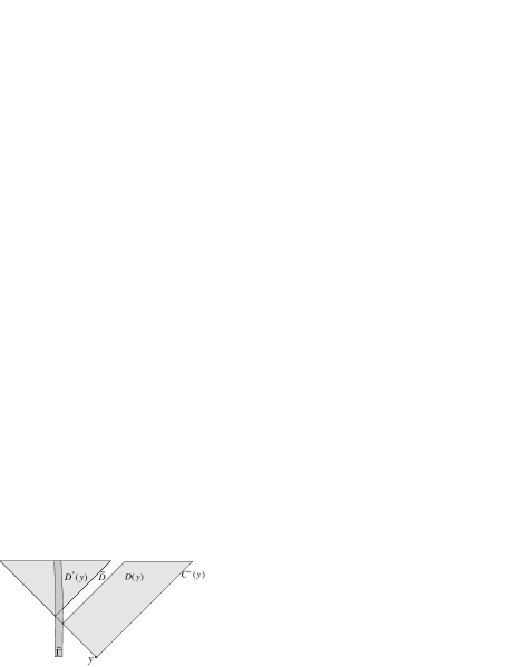
FIG. 2.: A diagram in Minkowski 2-spacetime: the regions where the character of the tail term is qualitatively different. $y$ is the source of electromagnetic waves and $\tilde{\Gamma}$ is the world-tube of gravitational source. The observer in the region $D(y)$ does not see any wavetail, the observer in $D^{*}(y)$ can see a wavetail of simple structure (37) whereas in the region $\tilde{D}(y)$ one can see a wavetail of the general form (30).

Eq. (44) leads to the conclusion that if the metric tensor satisfies the Einstein field equations, the tail term of the Green’s function in the first approximation in the spacetime domain $D^{*}(y)$ is completely determined by the four- momentum of the source of gravitation. The higher multipole moments of the source of gravitation, including the angular momentum, do not influence in this approximation the structure of ${\bf V}(x,y)$ (in the domain $D^{*}(y)$). A corresponding result for a scalar field has been presented in Ref. [38], and for a vector field in Ref. [33].

B Tail term for multipole solution

On the basis of Eq. (28), the tail term ${\cal V}_{\mu}^{a}$ of the retarded $2^{\mu}$-pole solution of Eq. (22) can be written as

$${\cal V}_{\mu}^{a}={1\over 2\pi}\int_{t_{0}}^{\tau(x)}V^{a}_{j;I(\mu)}(x,y(t))M_{\mu}^{I(\mu)j}(t)dt.$$ (45)

Next we will study the tail term ${\cal V}_{\mu}^{a}$ of a multipole solution in a weak gravitational field more closely. In a weak gravitational field the bivector field ${\bf V}(x,y)$ is determined by Eq. (39). In what follows we presume that the worldline $\xi$ of the source of electromagnetic waves remains outside the source of gravitational field, whereas $y(t_{0})$ and $y(t_{1})$ are points on the worldline $\xi$ of the wave source, $t_{0}$ and $t_{1}$ being, respectively, the proper time values when the source begins and terminates the emission. If the worldline $\xi$ of the wave source lies outside the world tube $\tilde{\Gamma}$ of the source of gravitation, i.e. $\text{supp}~{}\xi\cap\text{supp}~{}\tilde{\Gamma}=\emptyset$, and if $\text{supp}\,{\bf M}_{\mu}(t)\subset(t_{0},t_{1})$, then in the structure of the tail term ${\cal V}_{\mu}^{a}$ there appear features similar to the case of the tail term of the fundamental solution $\bf V$ discussed at the end of the last subsection.

To begin with, we divide the spacetime domain $J^{+}(y(t_{0}))\backslash\{\xi\}$ with $y(t)\in\xi$ into three subdomains:

$\displaystyle E:=\{x|x\in J^{+}(y(t_{0}))\backslash\{\xi\},\Sigma(y(t_{0}))\cap\tilde{\Gamma}=\emptyset\},$

$$E^{*}:=\{x|x\in J^{+}(y(t_{0}))\backslash\{\xi\},C^{+}(y(t_{1}))\cap\tilde{\Gamma}\subset\Sigma(y(t_{1})),$$ (46)

$$S(y(t_{1}))\cap\tilde{\Gamma}=\emptyset\},$$ (47)

$$\tilde{E}:=\{x|x\in J^{+}(y(t_{0}))\backslash\{\xi\},x\notin E,x\notin E^{*}\}.$$ (48)

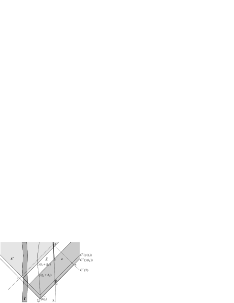
FIG. 3.: A diagram in Minkowski 2-spacetime: the regions $E$, $E^{*}$ and $\tilde{E}$ where the tail term of a wave pulse with finite duration behaves differently. The past light-cone $C^{-}(\bar{x})$ originating from the point $\bar{x}$ is represented by the dotted lines. The bold-faced part of the future light-cone $C^{+}(y(t_{0}))$ corresponds to the hypersurface $\Sigma(y(t_{0}))$ with $x=\bar{x}$, and the boundary of the hyperplane $\Sigma(y(t_{0}))$, i.e., $S(y(t_{0}))$ is seen as the two points $s$. $\tilde{\Gamma}$ is the worldtube of the source of gravitational field. $\xi$ is the worldline of the wave source which radiates during a finite proper time interval $[t_{0},t_{1}]$. $\lambda$ is the worldline of the observer. On the observer’s worldline $\lambda$ these intervals are indicated in bold where the observer can in principle see the direct pulse (the interval $[a,b]$) and the wave tail (the semi-interval $[c,\infty)$). During the interval $(b,c)$ on $\tilde{\xi}$ there occurs a blackout between the direct pulse and the wave tail.

In the subdomains $E$, $E^{*}$ and $\tilde{E}$ the character of the tail term of a wave pulse with finite duration is qualitatively different. (i) No-tail region. If $x\in E$, then also $x\in D(y(t))$ for every $t\in(t_{0},\tau(x))$. Hence it is valid that $V^{a}_{j}=0$, and consequently

$${\cal V}^{a}_{\mu}=0,\qquad\forall x\in E.$$ (49)

As $E\not=\emptyset$, there exist points in space, where the (fore)front of the wave is not simultaneously accompanied by the wave tail, the latter appearing after some time delay. To describe this effect in more detail, let us define the quantity $\tau_{0}(x,z)$ as a solution of the following set of equations:

$$\sigma(x,z)=0,\quad z\in C^{-}(x)\cap\tilde{\Gamma},$$ (50)

$$\sigma(z,y(\tau_{0}(x,z)))=0,\quad y(\tau_{0})\in C^{-}(z).$$ (51)

For further treatment are important the maximal and minimal values of the time interval $\tau(x)-\tau_{0}(x,z)$ (measured in the proper time of the wave source) for the fixed spacetime point $x$, viz.

$$\Delta_{1}(x):=\tau(x)-\text{max}~{}\tau_{0}(x,z),$$ (52)

$$\Delta_{2}(x):=\tau(x)-\text{min}~{}\tau_{0}(x,z).$$ (53)

The quantities $\Delta_{1}(x)$ and $\Delta_{2}(x)$ can be given a simple lucid interpretation by taking into account that an instantaneous wave pulse emitted by the wave source at $\text{max}~{}\tau_{0}(x,z)$ travelling at the speed of light reaches the spacetime point $x$ exactly as if it would first travel to the source of gravitation, reflect from there and further travel to the spacetime point $x$. In the case of $\text{min}~{}\tau_{0}(x,z)$ the reflection takes place precisely when the above-mentioned instantaneous wave pulse has passed the source of gravitation.

Obviously, in case $\tau(x)\leq t_{0}+\Delta_{1}(x)$, then $x\in E$ and ${\cal V}^{a}_{\mu}=0$.

(ii) Simple-tail region. If $\tau(x)\geq t_{1}+\Delta_{2}(x)$, then $x\in E^{*}$, and the structure of the tail term is determined only by the four-momentum of the source of gravitational field:

$${\cal V}^{a}_{\mu}=\!{1\over 8\pi^{2}}\!\!\int_{t_{0}}^{t_{1}}\!\!\!\!g^{a}_{j}(x,y(t))M_{\mu}^{I(\mu)j}(t)P^{b}\nabla_{b}\!\left[{1\over\sigma(x,y(t))}\right]_{;I(\mu)}\!\!\!dt.$$ (54)

Consequently, the higher multipole moments of the source of gravitation, among them the angular momentum, not influencing the structure of the wave tail.

(iii) General-tail region. To the domain $\tilde{E}$ corresponds the interval $(t_{0}+\Delta_{1}(x),t_{1}+\Delta_{2}(x))$ of the retarded time $\tau(x)$, and for these instants it is valid

$${\cal V}^{a}_{\mu}={1\over 2\pi}\int\limits_{t_{0}}^{\text{min}~{}(\tau(x)-\Delta_{1}(x),t_{1})}V^{a}_{j;I(\mu)}(x,y(t))M_{\mu}^{I(\mu)j}(t)dt,$$ (55)

where ${\bf V}$ is determined by Eqs. (39-41). Thus, in comparison with the direct pulse, the tail of the wave appears to the observer after the time delay $\Delta_{1}(x)$.

The particular case $\Delta_{1}(x)>t_{1}-t_{0}$ is also of interest. In it there occurs a time lapse of duration $\Delta(x)$ between the end of the principal pulse ($\tau(x)=t_{1}$) and the appearance of the wave tail, with

$$\Delta(x):=\Delta_{1}(x)-(t_{1}-t_{0}).$$ (56)

Hence, instead of a single pulse, the observer would see two clearly separable pulses: the principal one and the wave tail.

C Schematic representation of the geometry of wave tail generation

The purpose of this subsection is to provide a schematic plane spacetime representation of the geometry of wave tail generation. This subsection is meant as an illustration, the rest of this paper does not rely on it. For the sake of simplicity we make here the following simplyfing assumptions which are not used in our calculations: (i) the gravitational source is spherical and static, and (ii) the gravitational and wave sources, and the observer do not move with respect to each other.

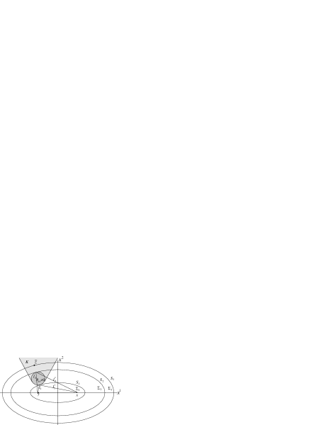
FIG. 4.: A schematic representation of the geometry of wave tail generation on a spacelike plane $x^{1}x^{2}$. Here $y$ is the wave source, $x$ is the observer, the darker shadowed circular disk is the gravitational source, and $K$ is the focusing region. The remaining components in the figure are explained in Sec. IV C.

In order to draw Fig.4 we have suppressed the time dimension and one space dimension. Thus all the images in Fig.4 are obtained by projecting the Minkowski spacetime onto a hypesurface $x^{0}=\rm{const}$, and then cutting the 3-space with $x^{1}x^{2}$. The plane of the figure is determined by locations of the wave source $y$, of the observer $x$ and of the center (not pointed out on the figure) of the gravitational source. The surface $S(y)$, which spreads with time, is the boundary of the ellipsoid of revolution $\Sigma(y)$, with foci at the locations of the observer $x$ and of the wave source $y$. The ellipses $S_{1}$ and $S_{2}$ are the intersections of the plane of the figure with the surface $S(y)$ that, respectively, correspond to the instants of time at which a delta-like wave pulse emitted by the wave source reaches and passes the source of gravitation. If the surface $S(y)$ has not yet reached the gravitational source, then ${\bf V}=0$ and there is no wave tail. If the surface $S(y)$ has passed the gravitational source, the source will forever remain inside the region of integration $\Sigma(y)$, while ${\bf P}(x,y)/8\pi=\rm{const}$ will be the $4$-momentum of the gravitational source and $F^{i}_{a}(x,y)=0$. The shadowed area $K$, which includes the source of gravitational field, corresponds to the region where the tail wave field is predominantly generated by gravitational focusing which deforms the direct wave fronts [15]. Thus we have the following picture. The wave source $y$ emits an instantaneous wave pulse. The direct pulse propagates along the direct route $yx$ to the observer $x$, after which there occurs a blackout before the arrival of the first tail contribution. The parts of the wave front which travel (along the routes $l_{1}$, $l_{2}$, etc.) to the points of the region $K$, scatter off (reflect) from there and then propagate (along $l_{1}^{*}$, $l_{2}^{*}$, etc.) to $x$ appearing to the observer as the tail wave.

To elucidate the introduced maximal and minimal time intervals, $\Delta_{1}$ and $\Delta_{2}$, let us again consider to the example presented in Fig.4. At the time $y^{0}=t_{0}$ the wave source emits a delta-like pulse. The evolution of the surface $S(y)$ is characterized by the time-varying semi-major $a$ and semi-minor $b$ axes which depend on the observer time $x^{0}$ as $a=(x^{0}-t_{0})/2$ and $b=(\sigma(x,y))^{1/2}/2$. The ellipses $S_{1},S_{2}$ and $S_{3}$ are the intersections of the plane of the figure with the surface $S(y)$ at times of observation $x^{0}_{1}=t_{0}+|\vec{x}-\vec{y}|+\Delta_{1}$, $x^{0}_{2}=t_{0}+|\vec{x}-\vec{y}|+\Delta_{2}$ and $x^{0}_{3}>x^{0}_{2}$, respectively. Here $|\vec{x}-\vec{y}|$ is the spatial separation between the wave source and the observer. The observer detects the direct pulse at the time $x^{0}_{0}=t_{0}+|\vec{x}-\vec{y}|$, the wave tail begins to appear at $x^{0}_{1}=t_{0}+l_{1}+l_{1}^{*}=x^{0}_{0}+\Delta_{1}$, and beginning from the time $x^{0}_{2}=t_{0}+l_{2}+l_{2}^{*}=x^{0}_{0}+\Delta_{2}$ the structure of the wave tail is determined by Eq. (39) with $F^{i}_{a}=0$. The time interval $\Delta_{1}=l_{1}+l_{1}^{*}-|\vec{x}-\vec{y}|$ is evidently equal to the difference of the propagation times of two pulses from the wave source to the observer: one arriving along the direct route and the other first travelling to the source of gravitation, reflecting from there and then reaching the observer.

D Radiative part of the electromagnetic wave tails

Let us examine the case in which the source of gravitation is spatially isolated and the distance of the source of waves from the source of gravitation is bounded. The tail term being a first-order small quantity, we can regard the spacetime as flat when discussing it and use Minkowskian coordinates whose origin lies inside the world tube of the source of gravitation. We denote the distance of the observer to the origin of the coordinates by $r$, and will also below use the following notation: if two functions $rA(x)$ and $rB(x)$ are equal in the limit $r\to\infty$, $\tau=\text{const}$, i.e. $\displaystyle\lim_{{r\to\infty\atop\tau=\text{const}}}(rA(x))=\lim_{r\to\infty\atop\tau=\text{const}}(rB(x))$, then we will write $A(x)\doteq B(x)$. The position vectors of the points $x$ and $y$ in three-space are denoted by $\vec{x}$ and $\vec{y}$, respectively.

Taking now into account that for an arbitrary finite $\tau$ are valid the asymptotic relations $\displaystyle\lim_{r\to\infty}\sigma(x,y(t))\sim r$, $\displaystyle\lim_{r\to\infty}\sigma_{;i}(x,y(t))\sim r$ and $\displaystyle\lim_{r\to\infty}\sigma_{;ik}(x,y(t))\sim O(1)$, we obtain from Eqs. (39-41) the relationship

$$V^{a}_{j;I(\mu)}(x,y(t))\doteq(-1)^{\mu}\sigma_{;i_{1}}(x,y(t))\dots\sigma_{;i_{\mu}}(x,y(t))\left({1\over\psi(x,t)}{d\over dt}\right)^{\mu}V^{a}_{j}(x,y(t)).$$ (57)

For brevity, in what follows we will not write explicitly the arguments of the functions depending both on the point $x$ as well as on the parameter $t$.

The radiative part of the wave tail which dominates at infinity can be written as

$${\cal V}^{a}_{\mu~{}\text{rad}}\doteq{(-1)^{\mu}\over 2\pi}\int\limits_{t_{0}}^{\tau(x)}\sigma_{;i_{1}}\dots\sigma_{;i_{\mu}}M_{\mu}^{I(\mu)j}(t)\left({1\over\psi}{d\over dt}\right)^{\mu}V^{a}_{j}dt.$$ (58)

Due to Eqs. (28) ja (14) the zeroth-order radiative part $Z^{a}_{\mu}$ of the $2^{\mu}$-pole solution can be written as

$$Z^{a}_{\mu}(x,y(\tau))\doteq{1\over 2\pi}\left[\left({1\over\psi}{d\over dt}\right)^{\mu}g^{a}_{j}{\sigma_{;i_{1}}\dots\sigma_{;i_{\mu}}\over\psi}M_{\mu}^{I(\mu)j}(t)\right]_{t=\tau(x)}$$ (59)

$$\doteq{1\over 2\pi}g^{a}_{j}(x,y(\tau))\left({1\over\psi(x,\tau)}{d\over d\tau}\right)^{\mu}{\sigma_{;i_{1}}(x,y(\tau))\dots\sigma_{;i_{\mu}}(x,y(\tau))\over\psi(x,\tau)}M_{\mu}^{I(\mu)j}(\tau).$$ (60)

On the basis of the last two relations, after integrating by parts the right hand side of Eq. (58) we obtain the following expression for ${\cal V}^{a}_{\mu~{}\text{rad}}$:

$${\cal V}^{a}_{\mu~{}\text{rad}}\doteq\int_{t_{0}}^{\tau(x)}\psi g^{i}_{b}V^{a}_{i}Z^{b}_{\mu}(x,y(t))dt$$ (61)

$$+\left\{\sum_{\nu=0}^{\mu-1}(-1)^{\mu-\nu}\left[\left({1\over\psi}{d\over dt}\right)^{\nu}V^{a}_{j}\right]\left({1\over\psi}{d\over dt}\right)^{\mu-\nu-1}{\sigma_{;i_{1}}\dots\sigma_{;i_{\mu}}\over\psi}M_{\mu}^{I(\mu)j}(t)\right\}_{t=\tau(x)},$$ (62)

where $Z^{b}_{\mu}(x,y(t)):=Z^{b}_{\mu}(x,y(\tau(x)))|_{\tau(x)=t}$.

We must point out that Eq. (62) contains $\mu+1$ terms, out of which the last $\mu$ ones are actually instantaneous. The first term in Eq. (62) is truly nonlocal, whereas the factor $\psi g_{b}^{i}V^{a}_{i}$ assigns most of the weight to the source’s recent past.

The truly nonlocal radiative wave-propagation correction

$$\tilde{\cal V}^{a}_{\mu~{}\text{rad}}:=\int_{t_{0}}^{\tau(x)}\psi g^{i}_{b}V^{a}_{i}Z^{b}_{\mu}(x,y(t))dt$$ (63)

takes an universal form which is independent of the multipole order. An analogous result in a weak Schwarzschild field in a slow-motion approximation has been earlier found in Ref. [10] (cf. also [26]). Our formula (63) generalizes this result in two ways. First, Eq. (63) is valid in case of an arbitrary weak gravitational field in the corresponding asymptotically flat spacetime. Second, there are no formal restrictions to the bounded motion of the wave source, e.g. the wave source can move with a relativistic speed. Due to the universal form of the tail term, Eq. (63) has a simple, but from the point view of observations essential, generalization. On the assumption that the local part $A^{a}(x,\tau)$ of a wave observable at infinity (or its zeroth-order radiative part) can be approximated with sufficient accuracy by the superposition of a finite number of multipole waves, it follows from Eq. (63) that the corresponding nonlocal radiative wave-propagation correction $E^{a}(x,\tau)$ has the following form:

$$E^{a}(x,\tau)=\int_{t_{0}}^{\tau(x)}\psi g^{i}_{b}A^{b}(x,t)V^{a}_{i}dt,$$ (64)

where $\psi$ is defined by Eq. (26).

For a source radiating in the pulsed mode the last formula enables us to comparatively simply (on the basis of the parameters of a recorded direct pulse and a presumable model of an astrophysical object) predict the physical parameters of the radiation tail and evaluate the possibilities of observational detection of the tail.

It should be emphasized that applicability of Eq. (64) does not depend on whether the source of radiation actually emits in the pulsed mode or pulses of radiation are present at the location of an observer due to the kinematics of the radiating system (e.g. the rotation of the directed radiation cone of a pulsar).

If $A^{b}(x,\tau)$ does not vanish merely during a finite time interval $t_{0}<\tau<t_{1}$ and the worldline of the source of radiation lies outside the world-tube of the source of gravitation, then the conclusions of Sec. IV B are also valid for the radiative part $E^{a}$ of the tail term. Thus, for example, if $\tau(x)\leq t_{0}+\Delta_{1}(x)$, then $E^{a}(x,\tau)=0$; if $\tau(x)\geq t_{1}+\Delta_{2}(x)$, then

$\displaystyle E^{a}(x,\tau)\!\doteq\!{1\over 4\pi}\!\int_{t_{0}}^{t_{1}}\!\!\!\!A^{a}(x,t)\psi(x,y(t))P^{b}\nabla_{b}\!\left({1\over\sigma(x,y(t)\!)}\right)dt$

$$\;\;\doteq{1\over 4\pi}\int_{t_{0}}^{t_{1}}{\sigma_{;b}(x,y(t))P^{b}\over\sigma(x,y(t))}{d\over dt}A^{a}(x,t)dt.$$ (65)

A matter of particular interest is the situation in which $\Delta_{1}(x)>(t_{1}-t_{0})$, as in this case there is a blackout during the time interval $\Delta(x)=\Delta_{1}(x)-(t_{1}-t_{0})$ between the end of the direct pulse and the appearance of the wave tail. The last fact considerably simplifies the observation methods for distinguishing the profile of the direct pulse from the general relativistic radiation tail originating from compact astrophysical binary systems. The relative intensity of the direct pulse and the wave tail, and the time delay (blackout) between them can yield essential additional information, independently of other methods, about the physical characteristics of a binary (the distance between the compact objects, the mass of the source of gravitation, the orientation of the plane of the orbit with respect to the observer, etc.).

From Eq. (65) it follows that the wave tail effect of the astrophysical systems radiating in the pulsed mode is predominatly caused by the low-frequency modes ($\omega\lesssim 2\pi/(t_{1}-t_{0})$) of the direct pulse. (Here the angular frequency $\omega$ of the radiation is measured in the proper time of the wave source.) The high-frequency waves reflecting from the spacetime curvature interfere and prevalently attenuate each other in the expression of the tail. Also important, from the point of view of observational detection, is the fact ensuing from Eq. (64) that the intensity and the time delay of the wave tail of radiation from a pulsed source moving on a circular orbit depend substantially on the mutual positions of the observer, the wave source and the source of gravitation. By comparing the profiles of the pulses emitted in different points of an orbit, one can distinguish in principle the contributions of the direct pulse and the tail even if there is no considerable time delay between the tail and the principal pulse. This circumstance is significant because in the case of most astrophysically realistic models the physical conditions necessary for the occurrence of a blackout in between the direct pulse and the wave tail will considerably decrease the intensity of the tail.

Let us now turn to the magnitude of electromagnetic radiative energy arriving after the direct pulse has passed, $\tau(x)>t_{1}+\Delta_{2}(x)$. The power ${dP\over d\Omega}$ radiated into the solid angle $d\Omega$ can be calculated as follows

$$I(\tau)\equiv{dP\over d\Omega}=-{r^{2}\over 4\pi}E^{a}_{,0}(x,\tau)E_{a,0}(x,\tau).$$ (66)

For further treatment it is reasonable to present Eq. (65) in a somewhat different form. In the proper reference frame of the source of gravitational field we have

$$E^{a}_{,0}\doteq-2M\int_{u(t_{0})}^{u(t_{1})}{[A^{a}_{,0}(x,\tau(x))]_{\tau(x)=t(u)}\over(u(\tau)-u)^{2}}du,$$ (67)

where $u(t):=y^{0}(t)-\vec{n}\cdot\vec{y}(t)$, $\vec{n}:=\vec{x}/|\vec{x}|$ and $M$ is the mass of the source of gravitational field. Below we will use notations $T:=u(t_{1})-u(t_{0})$, which is the duration of the direct pulse in the observer time, and $\tilde{\Delta}_{2}:=u(t_{1}+\Delta_{2}(x))-u(t_{1})$.

To get an idea of the magnitudes involved we construct an artificial example in which

$$A^{a}_{,0}(x,\tau(x))|_{\tau=t(u)}={1\over r}f^{a}(\upsilon,\phi)\Theta(u\!-u(t_{0}))\Theta(u(t_{1})\!-u).$$ (68)

Here $\Theta$ is the Heaviside distribution, $\upsilon,\phi$ are the polar angles determining the observer’s position and $f^{a}$ is an arbitrary vector function. From Eqs. (66-68) we obtain an estimate of the ratio of the intensity of the wave tail $I(t_{1}+\Delta_{2}(x))$ to the intensity of the direct pulse $I_{0}$ (the ratio of the densities of the energy fluxes at the observer’s location), namely

$${I(t_{1}+\Delta_{2}(x))\over I_{0}}=\left({2M\over\tilde{\Delta}_{2}(x)}\right)^{2}\left({T\over T+\tilde{\Delta}_{2}(x)}\right)^{2}.$$ (69)

We see that if $\tilde{\Delta}_{2}(x)$ is sufficiently small $(\tilde{\Delta}_{2}(x)\sim 2M)$, the intensity of the tail can be comparable with that of the direct pulse. Evidently, in this case we cannot confine ourselves to the first approximation but must instead additionally take into consideration the higher approximation(s).

To illustrate the above estimate, let us consider a wave source rotating in a circular orbit (of radius $r_{0}$) around a spherical source (of radius $r_{s}$) of gravitational field. The origin of the spatial coordinates is taken to coincide with the center of the source of gravitation. Under the conditions $\vec{n}\cdot\vec{y}(t_{1})<0$ and $r_{0}\gg d+r_{s}$, where $d:=r_{0}\sqrt{1-(\vec{n}\cdot\vec{y}(t_{1})/r_{0})^{2}}$, it follows from Eqs. (51) and (53) that

$$\tilde{\Delta}_{2}(x)\approx{(d+r_{s})^{2}\over 2r_{0}}+O(M).$$ (70)

Hence, if $r_{0}>r^{2}_{s}/4M$, then in case the wave pulse is emitted in the region of the geometric shadow of the source of gravitation or in its vicinity it is valid that $\tilde{\Delta}_{2}(x)\sim 2M$, and according to the estimate (69) the intensity of the tail can be of the same magnitude as the intensity of the primary pulse.

For the model under discussion it is also easy to find the ratio of the energy ${\cal E}$ transferred by the tail term (beginning from the time $t_{1}+\Delta_{2}(x)$) to the energy of the direct term ${\cal E}_{0}$, namely

$\displaystyle{{\cal E}\over{\cal E}_{0}}=\Bigl{(}{2M\over\tilde{\Delta}_{2}(x)}\Bigr{)}^{2}F\Bigl{(}{\tilde{\Delta}_{2}(x)\over T}\Bigr{)},$where

$\displaystyle F(\rho)=\rho+{\rho^{2}\over\rho+1}-2\rho^{2}\ln{\rho+1\over\rho}.$It is interesting to note that the function $F(\rho)$ has a maximum at $\rho\approx 0.638$.

FIG. 5.: The function $F(\rho)$ vs its argument $\rho$.

Therefore, for the given model the amount of energy transferred by the tail after the time $t_{1}+\Delta_{2}(x)$ is maximal if the duration of the direct pulse is $T\approx 1.57\tilde{\Delta}_{2}(x)$, and can in this case make up nearly $10\%$ of the energy of the direct pulse: ${\cal E}\approx 0.119{\cal E}_{0}(2M)^{2}/\tilde{\Delta}_{2}^{2}(x)$.

As the quantity ${\cal F}$ does not explicitly depend on the mass of the gravitational source, then its value for any particular case (as 0.119 for the present example) is primarily determined by the profile of the direct pulse and the spatial configuration of the system consisting of the wave source, gravitational source and the observer. Somewhat unexpected is the outcome that the magnitude of the factor $(2M/\tilde{\Delta}_{2})^{2}$, which characterizes the influence of the gravitational source, can be of the order $1$, even if the potential of the gravitational source is low everywhere, i.e. $2M\ll r_{s}$. This conclusion can be understood on the basis of Ref. [15] where it is shown that the tail field is predominantly generated by the direct field in those regions where gravitational focusing has deformed the geometry of the direct wave fronts (see the shadowed region in Fig. 4). The deformation is characterized by the focusing function $\alpha(\bar{z},y)$. If the points $\bar{z}$ and $y$ lie on a geodesic line which does not cross the gravitational source, then $\alpha(\bar{z},y)=0$. If the distance $r_{0}$ of the wave source from the gravitational source is much larger than the extension $r_{s}$ of the latter, then for the rays originating in the wave source and passing through the gravitational source it is valid $\alpha\sim Mr_{0}/r_{s}^{2}$. In the case of our example the condition $2M/\tilde{\Delta}_{2}\approx 1$ corresponds to $\alpha\sim 1$. Let us note that the last effect is not revealed by the traditional methods based on the expansion in terms of spherical functions, as in this case it is natural to choose the effective location of the wave source within the source of gravitation. Thus, $\tilde{\Delta}_{2}\approx r_{s}$ and $\alpha\sim M/r_{s}$, that is, the intensity of the tail is proportional to the square of the potential of the gravitational field on the surface of the source of gravitation.

Similar estimates for the energy of scalar and electomagnetic dipole wave tails in a strong Schwarzschild field have been found respectively in Refs. [39, 40].

E Constraints on applicability of the elaborated algorithm

Relying on Ref. [15], we will now briefly analyse limitations to applicability of the above results. Firstly, note that the conclusions of this paper were derived under the assumption that on the physically interesting spacetime domain the world function $\sigma$ is single-valued, i.e. the geodesics originating from the point $y$ do not cross. If this condition is not fulfilled, then the developed algorithms are not directly applicable. However, by virtue of the superposition principle, valid because of linearity of the wave equation, these algorithms can be applied even when the world function is a multiple-valued function. Then the correct classical Green’s function is the sum over all distinct elementary classical Green’s functions corresponding to all distinct geodesics between the points $x$ and $y$ (see also [20]).

Crossing of geodesics would be caused by gravitational focusing; and at the crossing point the exact factor $k(x,y)$ in ${\bf U}$ (see ([20])) would diverge. Thus, the criterion for no crossing is that $k(x,y)$ be finite along $C^{+}(y)$. Let us now consider our first-order expression (38). This expression for $k(x,y)$ can never diverge if the gravitational source is bounded. However, if the focusing function $\alpha(x,y)\equiv k(x,y)-1$ approaches unity, then the second- and higher-order effects will come into play, producing a divergence. Thus, the constraint $\alpha(x,y)<1$ for all $x$ and $y$ is necessary, on the one hand, for the first-order analysis to be valid; one the other hand, it simultaneously avoids crossing of geodesics.

For a wave-source in a circular orbit (the observer lying on the plane of the orbit), Eq. (38) gives $\text{max}~{}\alpha\sim(2M/r_{s})(2r_{0}/r_{s})$, where $M$ is the mass of the source of gravitation, $r_{s}$ is its linear size and $r_{0}$ is the radius of the orbit. In this case the constraint $\text{max}~{}\alpha<1$ is significant: it says that in order to avoid too much ray focusing, the wave-source and the gravitational source must not be too far apart

$${2M\over r_{s}}<{r_{s}\over 2r_{0}}.$$ (71)

Applying Eqs. (64), (65) and (67) to a particular model system, one should not overlook the fact that, although ${\bf E}$ is a first-order small quantity and therefore, when calculating the integrals involved the spacetime may be considered as a flat background; generally the retarded time $\tau(x)$ must be regarded as the retarded time on the curved spacetime because the integrands may be sensitive to the wave phase.

The quantities $\tilde{\Delta}_{2}(x)$ and $\tilde{\Delta}_{1}(x):=u(t_{0}+\Delta_{1}(x))-u(t_{0})$ offering their own inherent physical interest must generally also be calculated at least up to the accuracy of the first-order corrections.

Let us now consider in more detail the time intervals $\tilde{\Delta}_{2}(x)$ and $\tilde{\Delta}_{1}(x)$ for the binary system described at the end of Sec. IV C. We denote the origin of the coordinates at the center of the source of gravitation by $z$ and consider only the case in which the points $x$, $y$ and $z$ are aligned on a straight line. Evidently there are two possible cases: (i) the point $z$ is placed between the points $x$ and $y$, (ii) the point $y$ is placed between the points $x$ and $z$. Equations (51) and (53) yield the following conclusions. In the case (i) the time intervals $\tilde{\Delta}_{1}(x)$ and $\tilde{\Delta}_{2}(x)$ have maximal values:

$\displaystyle\text{max}~{}\tilde{\Delta}_{1}(x)=2(r_{0}-r_{s})+\chi_{1}(x),$

$\displaystyle\text{max}~{}\tilde{\Delta}_{2}(x)=2(r_{0}+r_{s})+\chi_{2}(x).$In the case (ii) the time intervals $\tilde{\Delta}_{1}(x)$ and $\tilde{\Delta}_{2}(x)$ have minimal values:

$\displaystyle\text{min}~{}\tilde{\Delta}_{1}(x)=0,\quad\text{min}~{}\tilde{\Delta}_{2}(x)={r_{s}^{2}\over 2r_{0}}+\chi_{3}(x).$Here the quantities $\chi_{\alpha}\sim 2M$, $\alpha=1,2,3$, denote the corrections caused by the Shapiro effect within the inner region of the binary system which are of the same order of magnitude as the Shapiro time delay between the points $y$ and $z$.

It is obvious that in Eqs. (64), (65) and (67) the corrections caused by the inner Shapiro effect may be neglected only in the low-frequency limit

$$\omega\ll{1\over 2M}.$$ (72)

The necessary condition (72) is also sufficient, if the inequality (71) is simultaneously satisfied.

V SUMMARY AND DISCUSSION

(i) On the basis of our earlier works [27, 24, 25], we developed simple recurrent formulas, i.e. Eq. (14), for calculating exact multipole solutions, i.e. Eq. (28), of the electromagnetic wave equation on the background of a curved spacetime which proceed from the classical Green’s function (i.e. the corresponding Hadamard coefficients).

(ii) The next main new contribution of this paper is formula (45) with (39) for the first-order tail term of the electromagnetic multipole wave in case of an arbitrary weak background gravitational field. From these formulas will follow a number of physically interesting effects.

Firstly, one can infer from Eqs. (39) the earlier known (see [34, 33]) necessary and sufficient condition for the validity of the Huygens’ principle (in the sense of Hadamard) in the first approximation, namely $R_{ab}=0$.

Secondly, if the gravitational field source is spatially isolated, then beginning from a certain instant of time the structure of the tail accompanied by a pulse of electromagnetic radiation is completely determined by the four-momentum of the source of gravitation, and the higher multipole moments, including the angular momentum, do not at all influence the structure of the tail in the first approximation. For the scalar wave equation and for the Green’s function of the electromagnetic wave equation essentially similar conclusions have been presented in Refs. [38] and [33].

Thirdly, in Sec. IV B we discussed a further consequence of Eq. (45), namely, the time delay effect of the tail with respect to the direct pulse. In the case of compact binary astrophysical objects the time interval (blackout) in between the direct pulse and the tail caused by delaying of the tail may be observable and can with the relative intensity of the tail give, independently of the other methods, essential information about the characteristics of the physical system (the distance between compact objects, the mass of the source of gravitation, the orientation of the plane of the orbit with respect to the observer, etc.). Earlier on the basis of the structure of the Green’s function of the wave equation in a weak Schwarschild field the time delay effect of the tail and its possible astrophysical implications have been indicated in the papers [3] and [4]. Let us mention that some unpublished calculations by the present authors demonstrate the occurrence of a similar delay effect also for linearized gravitational waves in the second approximation (cf. [5]). By the common approach in which the wave equation is solved by separating the angular variables the delay effect, as a rule, remains unrevealed. This is due to the circumstance that ensuing from the symmetry of gravitational field (Schwarzschild, Kerr etc.), the origin of the spherical coordinates whose worldline is simultaneously the worldline of the multipole radiation source lies inside the source of gravitation where the Ricci tensor does not vanish, $R_{ab}\not=0$.

(iii) It is valid in the first approximation that the nonlocal radiative wave-propagation correction at infinity takes a universal form (63) which is independent of the multipole order. A corresponding result in a weak Schwarzschild field in a slow-motion approximation has been published in [10]. Our Eq. (63) generalizes their result in two aspects. First, Eq. (63) is valid in case of an arbitrary weak gravitational field in the corresponding asymptotically flat spacetime. Second, there are no formal restrictions to the spatially bounded motion of the wave source, e.g. the motion of the wave source can be relativistic.

(iv) The intensity of the electromagnetic wave pulse emitted by the wave source within a compact binary in the vicinity of the geometric shadow of the source of gravitation can be of the same magnitude as the intensity of the direct pulse, and the energy carried away by the tail can amount to $10\%$ of the energy of the low-frequency modes of the direct pulse.

APPENDIX: NOTATION AND BASIC FORMULAS

1. We adopt the metric signature $(+,-,-,-)$ with the Latin indices running and summing from $0$ to $3$. To abbreviate the notation of repeated tensor indices, we introduce multi-indices, e.g. $A(\mu):=(a_{1}\dots a_{\mu})$, $I(\mu):=(i_{1}\dots i_{\mu})$, $P(\mu):=(p_{1}\dots p_{\mu})$, etc. We apply extensively the technique of two-point tensors (or bitensors) and follow closely the standard notation and index conventions [20]. To distinguish the tensor indices which refer to the point $x$ from those referring to the points $y$ and $z$ we use indices $a,b,\dots A(\mu),B(\mu),\dots$ at $x$, indices $i,j,\dots,I(\mu),J(\mu),\dots$ at $y$ and $p,q,\dots,P(\mu),Q(\mu),\dots$ at $z$. Thus $F^{a}_{I(3)}$ is a contravariant vector at $x$ and third-order covariant tensor at $y$. The index convention is also used for ordinary tensor fields, in which case it distinguishes the value of the component $v^{a}$ of a vector field ${\bf v}$ at $x$ from its value $v^{i}$ at $y$, and $G_{I(\mu)}$ denotes the covariant components of the tensor field ${\bf G}$ of rank $\mu$ at the point $y$.

2. Symmetrization and antisymmetrization of the tensor indices is denoted respectively by the parentheses and brackets. For example $t^{(ab)}:=(t^{ab}+t^{ba})/2$ and $t^{[ab]}:=(t^{ab}-t^{ba})/2$.

3. Ordinary differentiation is denoted by a comma (,). Covariant differentiation with respect to the Levi-Civita (metric) connection is denoted by $\nabla$ and semicolons, e.g. $\nabla_{x^{a}}f(x,y)=f_{;a}(x,y)$, $g^{ab}\nabla_{x^{b}}f(x,y)=f^{;a}(x,y)\;$ and $\nabla_{I(2)}f(x,y)=\nabla_{y^{i_{2}}}\nabla_{y^{i_{1}}}f(x,y)=f_{;i_{1}i_{2}}(x,y)$. Absolute differentiation along a line $z(\lambda)$ is denoted by an overdot, i.e. $\dot{w}^{i}=w^{i}_{;j}\dot{z}^{j}$.

4. We use a system of units in which the speed of light and the gravitational constant are equal to $1$.

5. The class of $C^{\infty}$ tensor fields of rank $m$ is denoted by ${\cal E}^{m}(\Omega)$ and the subspace of ${\cal E}^{m}(\Omega)$ consisting of fields with compact support by ${\cal D}^{m}(\Omega)$. A tensor-valued distribution ${\bf T}(x,y)\in{\cal D}^{\prime m}(\Omega)$ of rank $m$ at $x\in\Omega$ and of rank $k$ at $y\in\Omega$ is a continuous linear map ${\cal D}^{m}(\Omega)\to{\cal E}^{k}(\Omega)$. If $(\omega,\pi)$ is a coordinate chart such that $x,y\in\omega$ and ${\bf\Phi}\in{\cal D}^{m}(\omega)$, then each component of $(T_{I(k)}^{A(m)}(x,y),\phi_{A(m)}(x))$ is a (scalar-valued) tensor distribution (for a detailed discussion see [29]). A set $\Omega_{0}\subset\Omega$ is called past-compact if $J^{-}(x)\cap\Omega_{0}$ is compact (or empty) for all $x\in\Omega$. We denote the class of distributions in ${\cal D}^{\prime}(\Omega)$ with past-compact supports by ${\cal D}^{\prime+}(\Omega)$.

6. The world function biscalar $\sigma(x,y)\in C^{\infty}(\Omega\times\Omega)$ is defined by the equations

$$g^{ab}\nabla_{a}\sigma(x,y)\nabla_{b}\sigma(x,y)=4\sigma(x,y),$$ (73)

$$\sigma(x,y)=\sigma(y,x),\qquad\lim_{x\to y}\sigma=0.$$ (74)

The world function $\sigma(x,y)$ is numerically equal to the square of the geodesic arc length between the points $x$ and $y$, and is positive for timelike intervals and negative for spacelike intervals.

7. The propagator of geodetic parallel displacement (also called the transport bitensor) is defined as a bitensor field ${\bf g}(x,y)$ of rank $m$ at both $x$ and $y$, which satisfies, in local coordinates, the following differential equations and initial conditions:

$$\sigma^{;a}\nabla_{a}g^{I(m)}_{B(m)}(x,y)=0,$$ (75)

$$g^{I(m)}_{A(m)}(x,x)=\delta^{i_{1}}_{a_{1}}\dots\delta^{i_{m}}_{a_{m}}.$$ (76)

8. The surface distributions $\delta_{\pm}^{(\mu)}(\sigma(x,y)),\mu=0,1,2,\dots$ are defined by

$$(\delta_{\pm}^{(\mu)}(\sigma(x,y)),\phi(x)):=\lim_{\varepsilon\to+0}\left(-{\partial\over\partial\varepsilon}\right)^{\mu}\int_{C^{\pm}_{\varepsilon}(y)}\phi(x)\mu_{\sigma}(x)$$ (77)

for all $\phi\in C_{0}^{\infty}(\Omega)$, if $\mu=0$, and for all $\phi\in C_{0}^{\infty}(\Omega\backslash\{y\})$, if $\mu\geq 1$, where $\mu_{\sigma}(x)$ is a Leray form for which

$$d\sigma(x,y)\wedge\mu_{\sigma}(x)=\mu(x),$$ (78)

$\mu(x)$ being an invariant volume element and $C^{\pm}_{\varepsilon}(y)=\{x|x\in D^{\pm}(y),\sigma(x,y)=\varepsilon,\varepsilon>0\}$. In general, the integral (77) can be evaluated by means of a partition of unity subordinated to a covering of $\Omega$ by open coordinate neighbourhoods in each of which

$$\mu(x)=\sqrt{g(x)}dx^{0}\wedge dx^{1}\wedge dx^{2}\wedge dx^{3},$$ (79)

where $g(x):=|det(g_{ab}(x))|$ is the determinant of the metric tensor. The relevant properties of the surface distributions are given in [29, 41].

9. The $2$-form $\omega$ on the $2$-surface $S(y):=C^{+}(y)\cap C^{-}(x)$ in the integral (11) is defined by

$$d\sigma(z,x)\wedge d\sigma(z,y)\wedge\omega(z)=\mu(z),$$ (80)

where $\mu(z)$ is an invariant volume element on $M$.

10. The Heaviside distributions are defined by

$$(\Theta_{\pm}(\sigma(x,y)),\phi(x)):=\int_{J^{\pm}(y)}\phi(x)\mu(x),$$ (81)

where $J^{\pm}(y):=D^{\pm}(y)\cup C^{\pm}(y)$. The relevant properties of the Heaviside distributions can be found in Ref. [29, 41].

11. The scalarized van Vleck determinant is a biscalar which is defined by the equation

$$k(x,y):={{|\det\sigma_{;ai}(x,y)|^{1/2}}\over 4|g(x)g(y)|^{1/4}},$$ (82)

12. A $\mu$th-order Green’s function of the tensor wave operator ${\bf L}$ with respect to $(y,\Omega)$ is a tensor-valued distribution ${\bf G}(x,y)\in{\cal D}^{\prime 1}(\Omega)$ of rank $1$ at $x$ and of rank $\mu+1$ at $y$ which satisfies the equation

$$LG^{a}_{iJ(\mu)}(x,y)=(-1)^{\mu}\nabla_{B(\mu)}\!\left[g^{a}_{i}(x,y)g^{B(\mu)}_{J(\mu)}(x,y)\delta(x,y)\right],$$ (83)

where $g^{B(\mu)}_{J(\mu)}$ is the tensor propagator of geodetic parallel displacement.

REFERENCES

- [1] J. Hadamard, Lectures on Cauchy’s Problem (Yale University Press, New Haven, 1923).
- [2] P. Günther, Huygens’ Principle and Hyperbolic Equations (Academic Press, New York, 1988).
- [3] P. E. Roe, Nature. 227, 154 (1970).
- [4] P. C. Peters, Phys. Rev. D. 7, 368 (1973).
- [5] P. C. Peters, Phys. Rev. D 1, 1559 (1970).
- [6] L. Blanchet and B. S. Sathyaprakash, Class. Quantum Grav. 11, 2807 (1994).
- [7] L. Blanchet and T. Damour, Phys. Rev. D. 46, 4304 (1992).
- [8] L. Blanchet, Phys. Rev. D. 55, 714 (1997).
- [9] W. B. Bonnor and M. S. Piper, Class. Quantum Grav. 15, 955 (1998).
- [10] S. W. Leonard and E. Poisson, Phys. Rev. D. 56, 4789 (1997).
- [11] L. Blanchet, Class. Quantum Grav. 15, 113 (1998).
- [12] L. Blanchet and G. Schäffer, Class. Quantum Grav. 10, 2699 (1993).
- [13] E. Poisson, Phys. Rev. D. 47, 1497 (1993).
- [14] C. Cutler and E. E. Flanagan, Phys. Rev. D. 49, 2658 (1994).
- [15] K. S. Thorne and S. J. Kovacs, Astrophys. J. 200, 245 (1975).
- [16] W. B. Bonnor and M. A. Rotenberg, Proc. Roy. Soc. A289. 247 (1966).
- [17] J. M. Bardeen and W. H. Press, J.Math. Phys. 14. 7 (1973).
- [18] W. E. Couch, R. J. Torrence, A. I. Janis and E. T. Newman, J. Math. Phys. 9, 484 (1968).
- [19] A. J. Hunter and M. A. Rotenberg, J. Phys. A2, 34 (1969).
- [20] B. S. DeWitt and R. W. Brehme, Ann. Phys. 9, 220 (1960).
- [21] T. Regge and J. A. Wheeler, Phys. Rev. 108, 1063 (1957).
- [22] R. H. Price, Phys. Rev. D. 5, 2439 (1972).
- [23] E. W. Leaver, Proc. R. Soc. London A. 402, 285 (1985).
- [24] R. Mankin, R. Tammelo and T. Laas, Class. Quantum Grav. 16, 1215 (1999).
- [25] R. Mankin, R. Tammelo and T. Laas, Gen. Rel. Grav. 31, 537 (1999).
- [26] R. Mankin, R. Tammelo and T. Laas, Class. Quantum Grav. 16, 2525 (1999).
- [27] T. Laas, R. Mankin and R. Tammelo, Class. Quantum Grav. 15, 1595 (1998).
- [28] R. Mankin, T. Laas and R. Tammelo, Phys. Rev. D. 62, 041501(R) (2000).
- [29] F. G. Friedlander, The Wave Equation on a Curved Space-Time (Cambridge University Press, Cambridge, England, 1975).
- [30] W. G. Dixon, Proc. Roy. Soc. Lond. A. 319, 509 (1970).
- [31] H. Nariai, Nuovo Cimento, B35, 259 (1976).
- [32] R. Mankin and A. Ainsaar, Proc. Estonian Acad. Sci. Phys. Math. 46, 281 (1997).
- [33] R. Mankin and A. Sauga, Transactions of the Institute of Phys. Estonian Acad. Sci. 65, 41 (1989).
- [34] P. Günther, Wissen. Zeitschrift der Karl-Marx-Universität Math. Naturwissen. 14, 497 (1965).
- [35] B. S. DeWitt, C. M. DeWitt, Physics 1, 145 (1964).
- [36] C. M. DeWitt, C. R. Acad. Sci. (France) 256, 3827 (1963).
- [37] J. Colleau, C. R. Acad. Sci. (France) 256, 4596 (1963).
- [38] R. Mankin, Proc. Acad. Sci. ESSR. Phys. Math. 32, 351 (1983).
- [39] E. Malec, N. O’Murchada and T. Chamaj, Class. Quantum Grav. 15, 1653 (1998).
- [40] E. Malec, arXiv:gr-qc/0005130.
- [41] I. M. Gelfand and G. E. Shilow Generalized Functions Vol. I (Academic Press, New York, 1964).