A Quasilocal Hamiltonian for Gravity
with
Classical and Quantum Applications

Abstract

I modify the quasilocal energy formalism of Brown and York into a purely Hamiltonian form. As part of the reformulation, I remove their restriction that the time evolution of the boundary of the spacetime be orthogonal to the leaves of the time foliation. Thus the new formulation allows an arbitrary evolution of the boundary which physically corresponds to allowing general motions of the set of observers making up that boundary. I calculate the rate of change of the quasilocal energy in such situations, show how it transforms with respect to boosts of the boundaries, and use the Lanczos-Israel thin shell formalism to reformulate it from an operational point of view. These steps are performed both for pure gravity and gravity with attendant matter fields. I then apply the formalism to characterize naked black holes and study their properties, investigate gravitational tidal heating, and combine it with the path integral formulation of quantum gravity to analyze the creation of pairs of charged and rotating black holes. I show that one must use complex instantons to study this process though the probabilities of creation remain real and consistent with the view that the entropy of a black hole is the logarithm of the number of its quantum states.

AUTHOR’S DECLARATION FOR ELECTRONIC SUBMISSION OF A THESIS

I hereby declare that I am the sole author of this thesis. This is a true copy of the thesis, including any required final revisions, as accepted by my examiners.

I understand that my thesis may be made electronically available to the public.

Acknowledgements

I would like to thank Robert Mann, my supervisor, for all of his ideas, support, and help. I have had many useful conversations about quasilocal energy with other people as well and in particular with Eric Poisson, Richard Epp, and Jolien Creighton. A question from Eric led me to the thin shell work and the Hamiltonian part of his Physics 789 course greatly influenced my presentation of chapters 3 and 4. Jolien suggested the tidal heating calculation and collaborated with me on the paper where those results first appeared. The Natural Sciences and Engineering Research Council of Canada (NSERC), the Ontario provincial government through their Ontario Graduate Scholarships in Science and Technology (OGS-ST) programme, and the University of Waterloo have all provided financial support. Finally, I thank Valeri Frolov, John Wainwright, Ray MacLenaghan, Peter Hoffman, and Eric and Robb (again), who were my examining committee and made many constructive criticisms that have been incorporated into this final version of the thesis.

Chapter 1 Introduction

The conservation of energy is one of the most fundamental ideas in all of physics. As a principle, its history dates back three hundred years to Gottfried Wilhelm Leibniz whose philosophy of nature led him to propose that kinetic energy (which he called vis viva or “living force”) is conserved in an isolated system. This notion gained currency as the eighteenth century progressed and gradually widened to include various types of potential energy so that by the end of the century, the notion of conservation of vis viva was essentially equivalent to the conservation of total mechanical energy.

At the turn of the nineteenth century however, there was a large gap between the prevalent idea of energy conservation and how that concept is understood today. Most conspicuously, people didn’t realize that heat was a form of kinetic energy and instead believed that it was an independently conserved immaterial fluid called “calor”. In fact Sadi Carnot developed his theory of heat engines based on that concept and it was believed that the power of steam engines originated from flows of calor from high to low temperature just as water wheels are powered by the flow of water. It wasn’t until the middle of the nineteenth century that James Prescott Joule performed his decisive experiment to demonstrate that heat was also a form of energy and so paved the way for the modern formulation of energy conservation as expressed in the 1850’s by W. J. Macquorn Rankine’s definitive statement that “…the sum of the actual and potential energies in the universe is unchangeable …”. His notion of actual energy was identical to kinetic energy and in writing those words he was fully aware that heat is a form of kinetic energy.

With the recognition that heat is energy, a theory was required to explain under what circumstances work could become heat and vice versa. Recasting Carnot’s theory of heat engines in the light of the new ideas, scientists such as Rudolf Clausius and William Thomson (Lord Kelvin) developed thermodynamics to meet this need. As part of this science and to explain why a given amount of heat cannot be fully transformed into work, they developed the notion of entropy and the second law of thermodynamics which says that the entropy of a isolated system can never decrease. Then, to try to explain the macroscopic and general laws of thermodynamics at a microscopic and mechanical level, physicists such as Clausius, James Clerk Maxwell, and Ludwig Boltzman created statistical mechanics in the second half of the nineteenth century.

Now apart from emphasizing the central role that the notion of energy has played in physics, what makes the preceding bit of history relevant to this thesis is that the classical statistical mechanics that was developed could never fully explain the reality revealed by experience and experiment. For example, with its ideas of equipartition of energy this statistical mechanics could not successfully predict the low temperature heat capacities of an ideal gas, or much more dramatically, explain why the heat in a closed container doesn’t all shift into ultra-high frequency radiation (the “ultraviolet catastrophe”). Problems such as these ultimately led to the conception and birth of quantum mechanics.

Finally, momentarily leaving aside the thermodynamics, no discussion of energy is complete without a mention of Emmy Noëther’s celebrated theorem which states that the conserved quantities of a physical system are in one-to-one correspondence with the transformations which leave the value of its Hamiltonian (or Lagrangian) invariant. In particular, energy is conserved if and only if the Hamiltonian exhibits a time translation symmetry and angular momentum is conserved if and only if there is a rotation symmetry. Mathematically this result is straightforward and indeed almost trivial, but from a physical point of view its influence on theoretical physics since it was introduced early in the last century has been profound. Not surprisingly it will show up in my discussion of gravitational energy in the following chapters.

1.1 Gravity, energy, and thermodynamics

Today, the situation in gravitational physics is in some ways analogous to that of physics in general near the end of the nineteenth century. For almost thirty years physics has had a theory of black hole thermodynamics. It originated in the early 1970s with Bekenstein’s recognition that if the temperature of a black hole is proportional to its surface gravity and its entropy is proportional to the surface area of its horizon, then the laws of black hole mechanics are laws of thermodynamics [4, 5]. The first of these speculations was confirmed by Hawking’s discovery that a black hole emits radiation as a perfect black body with temperature proportional to its surface gravity [48] and the second supported by calculations which used the Euclidean path integral formulation of gravity (proposed by Gibbons and Hawking in [41]) to predict that a black hole has an entropy equal to one quarter of its surface area.

Thus, the classical laws of thermodynamics were extended to black holes with semiclassical calculations to bolster their interpretation and application. What was missing was a full theory of quantum gravity that could generate a statistical mechanics to explain them at a microscopic level. Now, the difficulties in constructing such a theory need not concern us here but the important point is that any successful candidate must have those laws as one of its predictions. Indeed in the quest for a theory of quantum gravity, the laws of black hole mechanics are one of the few clues to its final form. Recently the two leading candidates, string theory and canonical quantum gravity, have passed muster and predicted the entropy/area relationship (see for example [78] and [2] respectively) but the issue is by no means fully resolved.

As such, a proper formulation of the laws of black hole thermodynamics remains of great interest and that is one of the reasons why a good definition of energy is important in general relativity. To someone who is not directly involved in the field it would probably come as a surprise that such a definition doesn’t already exist. Afterall, I have just finished emphasizing how central is the role of energy in physics and general relativity has been part of that science for over 80 years. Thus, there has been no shortage of time in which to investigate how energy fits into the theory. What is more, the energy contained in the other fields of physics is well-understood. In general, all aspects of the energy content of a non-gravitational field may be described by a four-dimensional stress-energy tensor $T_{{\alpha}{\beta}}$. Roughly speaking, at any point in spacetime, the time-time components of this tensor define the field’s energy density, the time-space components describe the momentum carried by the field, and the space-space components describe the stresses associated with the field. Indeed, such stress-energy tensors play a central role in determining the general relativistic curvature of spacetime according to Einstein’s field equations which say that

$$G_{{\alpha}{\beta}}=8\pi T_{{\alpha}{\beta}},$$ (1.1)

where the Einstein tensor $G_{{\alpha}{\beta}}$ describes the curvature of spacetime. Of course, in general relativity gravity is curvature so the equations roughly say that matter curves spacetime and so creates gravitational fields.

Seeing these field equations one gets the first inklings that there might be a problem in defining energy in general relativity. Gravity plays the dual role of being a field and determining the spacetime in which it and all other fields live, so it seems likely that there could be problems in isolating its energy. Still and all, it seems possible that a stress-energy tensor could be conjured from somewhere. Such hopes are dashed by the equivalence principle. Recall that this states that there is no way for an observer making measurements entirely at a single point in spacetime to distinguish between her own acceleration and the effects of a gravitational field. Therefore there is no invariant way for a single observer to assign a “strength” to the gravitational field at a point and by extension no way to assign it an energy density. Thus there is apparently no way to define a purely local energy for gravity. An extended discussion of this point can be found in section 20.4 of reference [74].

How then are the laws of black hole mechanics defined if there is no way to define energy in a spacetime? Well, the answer is that the prohibition against a purely local definition of energy does not extend to the total energy of a spacetime. At least for asymptotically flat spacetimes, there are well known and accepted measures of the total energy such as the ADM [1] or Trautman-Bondi-Sachs [6] masses and it is usually one of these measures of energy that is used in the traditional formulations of black hole mechanics. However, this is not really a satisfactory way of proceeding since the thermodynamic system of interest is supposed to be the black hole itself rather than the entire, often infinite, spacetime of which it is a part. As an example consider a black hole spacetime which also contains a sprinkling of regular stars all situated many light years away from the hole and each other. Then, no one would argue that the stars should be considered as integral parts of the black hole system, yet the ADM energy would include the masses of those stars. Quasilocal definitions of gravitational energy attempt to meet this concern by defining the energy of just a part of the full spacetime while not attempting to fully localize the energy in a stress-energy tensor.

1.2 Quasilocal energy

A quasilocal definition of energy is a procedure that associates an energy with each closed and spacelike two-surface in a spacetime. Though there are many definitions of quasilocal energy in the literature (see for example [22, 55, 26, 34] and references contained those papers) a large subset of them can be characterized as Hamiltonian approaches. That is, they start with a Hamiltonian functional for finite three-surfaces in a spacetime which will generate the Einstein equations in the usual Hamiltonian way. Then the energy of the finite region is taken to be the value of that Hamiltonian evaluated thereon. Usually all bulk terms of the functional are proportional to constraints and so its numerical value evaluated on-shell is a functional on the boundary two-surface only. Given this property, the energy can’t really be said to be associated with the three-surface but instead is a property of the two-boundary alone. Any number of three-surfaces could be associated with that boundary, but which one actually is is completely irrelevant to the final evaluation. This property is in accord with the equivalence principle prohibition against a point-by-point localization of the energy. Since the energy can’t even be associated with a particular three-volume, it certainly can’t be assigned to individual points.

In some ways these definitions can be thought of as analogous to the Gauss law for electric charge. Just as that rule defines the electric charge contained by a closed two-surface from measurements of the electric field made at the surface, the quasilocal energies define the energy “contained” by a two-surface based on measurements of the gravitational field made at the surface.

One of the main aims of this thesis is to extend and generalize the popular Hamilton-Jacobi definition of quasilocal energy that was originally proposed by Brown and York [22]. Advantages of this definition include its appealing geometric form (discussed in some detail in chapter 3) and its natural interface with the path integral formulation of quantum gravity which allows one to do gravitational thermodynamics (briefly discussed in the next section and chapter 6, and in more detail in references [21, 19, 27]). Further, in common with other definitions of quasilocal energy, it can be shown to behave in ways that one would expect an energy to behave. For example it is additive, negative for binding energies, and in the appropriate limits (and spacetimes) it reduces to such total measures of energy as the ADM energy [22], the Trautman-Bondi-Sachs energy [16], and the Abbot-Deser energy [19]. In the small sphere limit in the presence of matter, it can be shown to recover intuitive notions of matter energy density [20].

The first part of this thesis reformulates the Brown-York definition into a pure Hamiltonian form and removes the slight dependence on the spanning three-surface from which their energy suffered. That is, I modify the Hamiltonian they proposed, show that it does indeed generate the correct field equations in the usual Hamiltonian way, and further show that its numerical value depends only on the values of fields at the bounding two-surface in a way that doesn’t care about what three-volume it contains. From there I show how the value of the Hamiltonian does depend on the motion of the observers measuring it, allow for the inclusion of Maxwell and dilaton fields, and show how the energy can be defined from an operational point of view.

Moving away from the mathematical formalism I get my hands dirty and try to develop an intuitive feel for the quasilocal energy by examining the distribution of energy in the standard static and spherically symmetric spacetimes. I then investigate naked black holes and calculate the energy flows that occur during gravitational tidal heating.

1.3 Path integrals, thermodynamics, and quantum tunnelling

The last part of the thesis deals with a quantum application of the Hamiltonian work. As noted above, the quasilocal formalism of Brown and York naturally combines with the path integral formulation of quantum gravity and thereby gives some insights into gravitational thermodynamics. Recall that in general, path integral versions of quantum mechanics calculate the probability that a quantum system passes from an initial state $X_{1}$ to a final state $X_{2}$ by considering all conceivable “paths” that the system can take between the two states (not just those that satisfy classical equations of motion). The action of each of those paths can be computed using a classical Lagrangian action functional and then, up to a normalization factor, the probability amplitude that the system takes a specific path is $e^{-iI}$ where $I$ is the action of the path. Then, the sum of all of these probability amplitudes is the probability amplitude that the system will pass to the final state $X_{2}$. There are a myriad of unsolved problems involved in rigorously defining these integrals, but nevertheless history has shown that many physical insights can be gained through their judicious use.

The problems of mathematical rigor are even more serious for path integral gravity than for regular quantum mechanics, but all the same its usefulness as a conceptual and provisional computational tool remains. In particular, as is usual with path integrals, one can use it to study thermodynamics by viewing the “paths” as members of a thermodynamic ensemble and so reinterpret the path integrals in terms of partition functions.

The connection with the quasilocal formalism arises because the classical behaviour of a system is not sufficient to specify the action functional that should be used to assign the probability amplitude to each path. However, it turns out that the choice of an action functional also corresponds to a choice of restrictions on the ensemble of paths considered. The Brown-York formalism provides a convenient way to see those restrictions from a thermodynamic perspective. With this insight one can associate each action functional with a specific thermodynamic partition function (for example grand canonical, canonical, or microcanonical) as was first discussed in reference [21].

That said, one can also use the path integrals in their original form to estimate the probability that a quantum event will occur. In this case, one must recognize that the action functional still places restrictions on the physical properties of the paths considered and so should be chosen to conserve essential physical properties (such as the angular momentum or electric charge of a spacetime) through the quantum transition.

As a specific application, in recent years there has been a considerable interest in black hole pair production. Inspired by the well understood particle pair production of quantum field theory (for example $2\gamma\rightarrow e^{+}+e^{-}$), theorists have investigated the corresponding phenomenon for black holes and studied the possibility that a spacetime with a source of excess energy will quantum tunnel into a spacetime containing a pair of black holes. The earliest investigations considered pair creation due to background electromagnetic fields [30, 29, 39, 49] but since then have been extended to include pair creation due to cosmological vacuum energy [71, 14], cosmic strings [53, 32, 31], and domain walls [23, 69, 70]. In all cases the chance of such an event happening has been found to be extremely small, but perhaps an equally interesting outcome of the calculations has been the evidence that they have provided that black hole entropy does indeed correspond to the number of quantum states of the hole.

In the last part of the thesis I show how the pair creation results can be extended to include pairs of rotating black holes, which were not considered in the above referenced papers. This is quite an involved process which starts with the identification of classical solutions to the Einstein equations that properly describe pairs of black holes in the appropriate context. From there instantons are constructed from the classical solutions that will be used to approximate the path integrals and it is seen that requirements of regularity restrict the possible physical parameters of the created spacetime. The Brown-York formalism is used to choose the correct action for use in each situation and finally, with all of the preparation completed, I calculate and interpret the creation probabilities.

1.4 Overview

With these ideas in mind I now outline the rest of the thesis. As its name implies, chapter 2 establishes the background for the work that follows. Much of it is a review of well-known ideas and results but it will serve to refresh these ideas for the reader who is not especially familiar with this area of general relativity and establish notation and sign conventions. Since I will be working with a Hamiltonian formulation of general relativity, section 2.1 explains how a spacetime may be foliated into “instants” of time and how a vector field is set up to define the “flow of time” from instant to instant. I focus on a finite region of that spacetime and discuss its boundaries and the fields on those boundaries in some detail as well as give a physical interpretation of the boundaries as being defined by the history of a closed two-surface of observers. Extending the spacetime foliation to the timelike boundary, I foliate it with closed two-surfaces which define the observers’ notion of simultaneity. The quasilocal energy will be defined for these surfaces.

Section 2.2 reviews the field equations for fields of interest to this thesis. Specifically they are gravity, electromagnetism, and a dilaton field where a coupling exists between the dilaton and Maxwell fields. First examining these from a covariant four-dimensional perspective, I then review how they become constraint and evolution equations if they are projected into the leaves of the time foliation. I discuss how one-half of the Maxwell equations are implied by the assumption that a gauge potential exists, a simple fact that will have larger consequences later on, and discuss duality for these three fields.

With this theoretical stage set, chapter 3 begins the main work of the thesis. Starting with a modified Einstein-Hilbert action for gravity, section 3.1 briefly reviews how it variation produces the standard field equations for gravity. The action (proposed by Geoff Hayward in ref. [54]) differs from the classical Einstein-Hilbert action in that it is formulated for a finite region of spacetime bounded by a combination of spacelike and timelike hypersurfaces and disagrees with the one used by Brown and York in that it allows for those boundaries to be non-orthogonal.

From that action, subsection 3.2.1 derives a Hamiltonian functional defined on the slices of the time-foliation of the spacetime. This Hamiltonian differs from the Brown-York Hamiltonian in that it does not restrict the time foliation to be orthogonal to the timelike boundary. It is noted that even though the functional is defined for a finite region of a spatial three-surface, its actual on-shell numerical value depends only on the fields at the boundary of that surface and how they are evolving in time. It is indifferent to what three-surface it bounds. This means that a quasilocal energy derived from the Hamiltonian really is a functional of the boundary two-surface only; a fact which is crucial for its proper definition since there is no natural way to uniquely associate a spanning three-surface with that boundary (or for that matter even guarantee that such a surface exists). Thus, this approach differs markedly from that taken by Hawking and Hunter in ref. [51] which required reference terms to remove the dependence of their Hamiltonian on the intersection angle between the foliation surfaces and timelike boundary.

With the proposed Hamiltonian functional in hand, subsection 3.2.2 confirms that it really is a properly defined Hamiltonian (this is the first time that this has been explicitly demonstrated) and shows that, as would be expected, the calculated variation of the Hamiltonian is in accord with the full variation of the action functional as considered in such papers as [22, 10].

Section 3.3 presents a definition of quasilocal energy in terms of the quasilocal Hamiltonian of the previous section. Its exact form is dependent on the time four-vector that determines the evolution of the boundary observers and it is seen that if that vector field is a Killing vector field for the induced metric on the boundary of the spacetime, then the quasilocal energy is a conserved quantity. A special case of the general quasilocal energy where the observers are stationary relative to the foliation hypersurfaces and measure proper time is considered and geometrical interpretations of that energy are discussed. Transformation laws for the quasilocal quantities with respect to boosts of the measuring observers are derived and investigated in section 3.4. These laws are shown to be Lorentz-like and a comparison is made with corresponding laws from special relativity.

Next, section 3.5 defines reference terms for the quasilocal energy of the previous sections. These terms are necessary because without them the quasilocal energy of a spherical region of flat space is non-zero and actually diverges as the radius of such a sphere goes to infinity. Within the quasilocal formalism there is quite a lot of freedom to define these reference terms and the choice of a particular one is essentially a choice of where to set the zero-level of the energy. I examine three choices of reference terms, starting with the original Brown-York term which is defined by embedding the instantaneous two-surface of observers into a reference three-space. A well recognized problem with this term is that it is not always defined and I point out that it also runs into problems for boosted observers in flat space. From there I discuss an alternate proposal involving embedding the instantaneous two-surface of observers into a four-dimensional reference space (discussed in [10, 11] and from a different perspective in [34]). It is more likely to exist than the three-dimensional proposal but unfortunately is not uniquely defined. Finally, I briefly comment on the so-called intrinsic reference terms that have recently been inspired by the AdS-CFT correspondence.

The chapter ends with section 3.6 which investigates the close relationship between the quasilocal energy and the thin shell formalism of Israel [59]. I show that there is an exact correspondence between the mathematics of the quasilocal energy and the thin shell formalism. This means that for a two-surface of observers with a specified time evolution in a given spacetime, the quasilocal energy with the two-into-four reference terms discussed above is defined if and only if that two-surface could be replaced with a thin shell of matter so that outside of the shell the spacetime would be unchanged while inside it would be isometric to a part of the reference space. The quasilocal energy measured by the observers is exactly equal to the total matter stress-energy of the thin shell. This equivalence means that one can reinterpret the (modified) Brown-York quasilocal energy from an operational point of view. That is, the quasilocal energy “contained” by a two-surface could be defined as the matter stress-energy required to reproduce that spacetime outside of a matter shell that is isometric to the two-surface and embedded in the reference space.

Though similar in length to the previous one, chapter 4 can be summarized quite a bit more quickly since it covers much the same ground except that this time Maxwell and dilaton matter fields are included in the mix. It starts in section 4.1 with a review of the Lagrangian action whose variation will generate all of the field equations. From there, subsection 4.2.1 derives a Hamiltonian functional from that Lagrangian action and it is noted that the assumption that a single gauge potential exists over the region being studied implies not only two of the Maxwell equations, but also that no magnetic charge can exist in that region. Subsection 4.2.2 checks that the proposed functional really is a proper Hamiltonian and again compares the variation of the Hamiltonian with previously calculated action variations [27, 28, 11]. Section 4.3 reviews conserved charges, reference terms, transformation laws, and the thin shell correspondence when the matter fields are included along with the gravitational field. Finally, in recognition of the fact that the formalism as constituted cannot handle magnetic charges, section 4.4 uses duality to define an action and Hamiltonian that can handle those charges, though in doing so it loses the ability to deal with electric charges.

Chapter 5 applies the work of the previous two chapters to several spacetimes both to gain insight into the quasilocal energy and to demonstrate its utility. Section 5.1 is targeted mainly towards the first goal as it examines Schwarzschild and Reissner-Nordström spacetimes. It starts with static and spherically symmetric sets of observers and shows that the quasilocal energies that they measure are physically reasonable though not entirely in accord with intuition. Interestingly it is seen that the definition of the quasilocal energy derived for a purely gravitational field appears to also include contributions from matter fields. The extra terms generated by matter fields are gauge dependent and are not directly related to the physical configuration of the system but instead seem to give the potential energy for the system to exist relative to an (almost) arbitrarily set gauge potential. The next section considers radially boosted observers which the original Brown-York formalism couldn’t easily handle and so demonstrates the nonorthogonal formalism. Finally a spherical set of “z-boosted” observers is considered for Schwarzschild space and interesting but slightly enigmatic results are obtained.

Section 5.2 applies the formalism to study naked black holes (first discussed by Horowitz and Ross in [56, 57]). These are massive, near-extreme, Maxwell-dilaton black holes that are characterized by how different sets of observers feel gravitational tidal forces close to the event horizon. Specifically, static observers measure relatively small transverse tidal forces while those who are infalling on radial geodesics measure huge (though not divergent) forces. Though at first thought this might not seem to be especially surprising, it should be kept in mind that equivalent observers near to similar Reissner-Nordström black holes all measure small tidal forces irrespective of their radial motion. I calculate the quasilocal energies measured by corresponding spherical sets of observers and find that the static ones measure a very large quasilocal energy while the infalling ones measure it to be extremely small. I explain all of these measurements in terms of the geometry of the naked spacetimes.

The final classical application is found in section 5.3 where I apply the formalism to calculate energy flows during gravitational tidal heating. The prototypical example of this in our own solar system is found in Jupiter and its moon Io, where the gravitational tidal forces provide the energy that powers Io’s volcanism. I successfully reproduce the results of energy flow calculations that in the past have been done with Newtonian and stress-energy pseudo-tensor [80] methods. The calculation is cleaner than the pseudo-tensor calculations and has the added advantage of providing a simple geometric interpretation of gauge ambiguities in the energy flow. Thus, this section can be viewed both as an application of the quasilocal formalism and as an additional check on its physical relevance.

Chapter 6 contains a quantum mechanical application of the formalism as it applies it to the pair production of charged and rotating black hole pairs in a cosmological background. It begins with a brief review of the Euclidean path integral formulation of quantum gravity in section 6.1. Section 6.2 examines the classical spacetimes that describe pairs of charged and rotating black holes in a cosmological background. It starts with the generalized C-metric of Plebanski and Demianski [79] which can be interpreted as describing a pair of charged and rotating black holes accelerating away from each other in a cosmological background, and then shows that matching the acceleration of the holes to that of the rest of the universe (as is demanded by conservation of energy) reduces this metric to the Kerr-Newman-deSitter (KNdS) metric. Thus, those will be the class of spacetimes that I aim to create and so I examine them in some detail, working out the allowed range of their physical parameters and examining limiting cases. Traditionally it has been asserted that only spacetimes in full thermodynamic equilibrium can be created by quantum tunnelling processes, so I finish off by considering the various KNdS spacetimes from this point of view. I show that three limiting cases of the KNdS spacetime, the cold limit (which corresponds to a pair of extreme black holes), the Nariai limit (where the outer black hole and cosmological horizon become coincident), and an ultracold limit (the overlap of the cold and Nariai limits) are in thermal (but not full thermodynamic) equilibrium as are a class of non-extreme black holes that are dubbed lukewarm (where the outer black hole and cosmological horizons simply have the same temperature). If the rotation parameter is set to zero, then these reduce to equivalent cases considered in extant non-rotating calculations.

Section 6.3 assembles instanton solutions to mediate the creation of each of the classes of KNdS spacetimes that are in thermal equilibrium. These instantons have complex metrics, in contrast with the usual ones used to create non-rotating pairs of black holes. I show that this is a necessary feature of the instanton metrics if one requires that these solutions match onto the corresponding Lorentzian ones along a spacelike hypersurface. Finally I construct the actual instantons treating the non-degenerate two horizon (lukewarm and Nariai), non-degenerate single horizon (cold, ultracold I), and zero horizon (ultracold II) cases separately. I note that only thermal (rather than full thermodynamic) equilibrium is required to construct a smooth instanton.

Section 6.4 examines the instantons to identify their essential features and then uses the Brown-York formalism to select the actions that will preserve those characteristics during the quantum tunnelling. Then with that action in hand section 6.5 evaluates those actions for the instantons and so finds the probability for a pair creation event to occur. It is shown that the probability of pure deSitter space tunnelling into a spacetime containing a pair of black holes with opposite spins and electric/magnetic charges is proportional to $e^{-\Sigma{\mathcal{A}}_{i}/4}$ where $\Sigma{\mathcal{A}}_{i}$ is the sum of the areas of the non-degenerate horizons in the created spacetime. This is in accord with the corresponding results for non-rotating holes [71] as well as an interpretation of black hole entropy as the logarithm of the number of quantum states of the hole. Section 6.6 shows how the methods that I have used compare with the procedures that other people have used.

Finally, chapter 7 attempts to summarize the results of the thesis, put them into some perspective, and discusses future work related to the topics of this thesis.

Chapter 2 Set-up

This chapter sets the stage on which the rest of the thesis will play. In the first section I define a quasilocal region of space, show how it may be foliated, and define a variety of geometric quantities that will be used extensively in the rest of the thesis. The second section reviews the interlocking field equations for gravity, electromagnetism, and the dilaton field in their full four-dimensional and projected three-dimensional forms. It further discusses electromagnetic potentials and the duality inherent in the electromagnetic and dilaton fields. Much of this chapter is a review of well known facts but it serves to establish notation and cast some of these ideas in a new light.

2.1 The geometric background

Let $M$ be a compact and topologically trivial region of a four-dimensional spacetime ${\mathcal{M}}$. It is specified to be the region bounded by two spacelike surfaces $\Sigma_{t1}$ and $\Sigma_{t2}$ (each homeomorphic to ${\mathbb{R}}^{3}$) and a timelike surface $B$ (homeomorphic to ${\mathbb{R}}\times S^{2}$). Such a region is depicted schematically in figure 2.1. Let $M$ be foliated with a set of three-dimensional spacelike surfaces $\{\Sigma_{t}\}$, labelled by a time coordinate $t$, such that $\Sigma_{t1}$ and $\Sigma_{t2}$ are leaves of the foliation. This then induces a corresponding foliation of $B$ by spacelike two-surfaces $\{\Omega_{t}\equiv\Sigma_{t}\cap B\}$ each with topology $S^{2}$. Finally, in association with the foliations define a smooth timelike vector field $T^{\alpha}$ such that $T^{\alpha}\partial_{\alpha}t=1$ and is tangent to $B$. These conditions are not sufficient to uniquely specify $T^{\alpha}$, so there is a certain arbitrariness in its definition.

Figure 2.1: A three-dimensional schematic of the Lorentzian region $M$, assorted normal vector fields, and typical elements of the foliation.

Intuitively one can think of $B$ as defining the history of a set of observers and each $\Sigma_{t}$ as defining an “instant” in time. Then each $\Omega_{t}$ defines an “instantaneous” configuration of those observers and in the regular way, I will say that $\Omega_{t1}$ “happens” before $\Omega_{t2}$ if $t_{1}<t_{2}$. Further $T^{\alpha}$ can be thought of as the (unnormalized) four-velocity of the observers and so $B$ can be viewed as the history of a set of observers who started out in the configuration $\Omega_{t1}$ and then evolved through time with $T^{\alpha}$ as their four-velocity. Because $T^{\alpha}$ isn’t normalized the time $t$ doesn’t correspond to proper time. The freedom in the definition of $T^{\alpha}$ corresponds to how individual observers can evolve differently while leaving their evolution as a set invariant.

Note that while a $\Sigma_{t}$ foliation surface uniquely specifies a corresponding $\Omega_{t}$, the converse isn’t true. Any number of $\Sigma_{t}$ foliations can be defined that are compatible with a given $\Omega_{t}$ foliation. In fact in spite of the way that the foliations have been set up in this section, a main goal of this thesis is to show that only the foliation of $B$ is important. The foliation of the rest of the spacetime is irrelevant, basically because there are no observers in the interior of $B$ to define it. The only observers are thought of as residing on the boundary $B$.

Up to this point no real use has been made of a metric. Terms like spacelike and timelike have been used for clarity but everything could equally well have been formulated in terms of a manifold without metric. Now however, I’ll introduce a signature $+2$ metric field $g_{{\alpha}{\beta}}$ over $M$. With this metric one can define a (unit normalized) forward-pointing timelike vector field $u^{\alpha}$ normal to the $\Sigma_{t}$ surfaces as well as induce a spatial metric field $h_{{\alpha}{\beta}}\equiv g_{{\alpha}{\beta}}+u_{{\alpha}}u_{{\beta}}$ on those surfaces. Then, one can project $T^{\alpha}$ into its components perpendicular and parallel $\Sigma_{t}$. Namely

$$T^{\alpha}=Nu^{\alpha}+V^{\alpha},$$ (2.1)

where $N$ and $V^{\alpha}$ are called the lapse function and shift vector field respectively and $V^{\alpha}u_{\alpha}=0$. Conversely one can define the spacetime metric in terms of the spatial metric, lapse, shift, and time vector field by

$$g^{{\alpha}{\beta}}\equiv h^{{\alpha}{\beta}}-\frac{1}{N^{2}}(T^{\alpha}-V^{\alpha})(T^{\beta}-V^{\beta}).$$ (2.2)

Define unit normal vector fields for the various hypersurfaces. Already $u^{\alpha}$ has been defined as the future-pointing timelike unit normal vector field to the $\Sigma_{t}$ surfaces. Similarly, define ${\bar{u}}^{\alpha}$ as the future-pointing timelike unit normal vector field to the surfaces $\Omega_{t}$ in the timelike hypersurface $B$. The spacelike outward-pointing unit normal vector field to $\Omega_{t}$ that is perpendicular to $u^{\alpha}$ (and thus in the tangent bundle $T\Sigma_{t}$) is $n^{\alpha}$ and the corresponding normal vector field to $\Omega_{t}$ perpendicular to ${\bar{u}}^{\alpha}$ is ${\bar{n}}^{\alpha}$ which is also the outward-pointing unit normal vector field to $B$.

Next define the scalar field $\eta={\bar{u}}^{\alpha}n_{\alpha}=-u^{\alpha}{\bar{n}}_{\alpha}$ over $B$. If $\eta=0$ everywhere, then the foliation surfaces are orthogonal to the boundary $B$ (the case dealt with in refs. [22, 50]) and the barred vector fields are equal to their unbarred counterparts. If $\eta\neq 0$ then ${\bar{u}}^{\alpha}$ and ${\bar{n}}^{\alpha}$ may be written in terms of $u^{\alpha}$ and $n^{\alpha}$ (or vice versa) as,

$${\bar{n}}^{\alpha}=\frac{1}{\lambda}n^{\alpha}+\eta u^{\alpha} {\bar{u}}^{\alpha}=\frac{1}{\lambda}u^{\alpha}+\eta n^{\alpha},$$ and

or,

$$n^{\alpha}=\frac{1}{\lambda}{\bar{n}}^{\alpha}-\eta{\bar{u}}^{\alpha} u^{\alpha}=\frac{1}{\lambda}{\bar{u}}^{\alpha}-\eta{\bar{n}}^{\alpha},$$ and (2.4)

where $\lambda^{2}\equiv\frac{1}{1+\eta^{2}}$. $\eta$ and $\lambda$ may also be written without direct reference to the barred normals. To do that first define

$$v_{\vdash}\equiv(V^{\alpha}n_{\alpha})/N,$$ (2.5)

which is the three-velocity in the direction $n^{\alpha}$ of an object with four-velocity $T^{\alpha}$ as measured by an observer with four-velocity $u^{\alpha}$. Then,

$$\eta\equiv v_{\vdash}/\sqrt{1-v_{\vdash}^{2}} \lambda=\sqrt{1-v_{\vdash}^{2}}.$$ and (2.6)

These quantities then begin to look like the terms that appear in special relativistic Lorentz transforms. This correspondence will be explored in some detail in section 3.4.

On the surface $B$ one may write,

$$T^{\alpha}={\bar{N}}{\bar{u}}^{\alpha}+{\bar{V}}^{\alpha},$$ (2.7)

where

$${\bar{N}}\equiv\lambda N=\sqrt{N^{2}-[V^{\alpha}n_{\alpha}]^{2}} {\bar{V}}^{\alpha}\equiv\sigma^{\alpha}_{\ {\beta}}V^{\beta}=V^{\alpha}-[V^{\beta}n_{\beta}]n^{\alpha}$$ and (2.8)

are respectively labelled the boundary lapse and the boundary shift. This split is possible because $T^{\alpha}$ on $B$ has been restricted to lie in the tangent bundle $TB$. Equivalently, $B$ is the history of the observers $\Omega_{t}$ and $T^{\alpha}$ is their four-velocity, so naturally $T^{\alpha}\in TB$ on $B$. In any case $T^{\alpha}{\bar{n}}_{\alpha}=0$.

Next consider the metrics induced on the hypersurfaces by the spacetime metric $g_{{\alpha}{\beta}}$. Just as $h_{{\alpha}{\beta}}\equiv g_{{\alpha}{\beta}}+u_{\alpha}u_{\beta}$ is the metric induced on the $\Sigma_{t}$ surfaces, the other metrics may also be written with respect to the normals. $\gamma_{{\alpha}{\beta}}\equiv g_{{\alpha}{\beta}}-{\bar{n}}_{\alpha}{\bar{n}}_{\beta}$ is the metric induced on $B$ and $\sigma_{{\alpha}{\beta}}\equiv h_{{\alpha}{\beta}}-n_{\alpha}n_{\beta}=\gamma_{{\alpha}{\beta}}+{\bar{u}}_{\alpha}{\bar{u}}_{\beta}$ is the metric induced on $\Omega_{t}$. Raising one index of these metrics defines projection operators into the corresponding surfaces. These have the expected properties: $h^{\alpha}_{\ {\beta}}u^{\beta}=\gamma^{\alpha}_{\ {\beta}}{\bar{n}}^{\beta}=\sigma^{\alpha}_{\ {\beta}}u^{\beta}=\sigma^{\alpha}_{\ {\beta}}n^{\beta}=\sigma^{\alpha}_{\ {\beta}}{\bar{u}}^{\beta}=\sigma^{\alpha}_{\ {\beta}}{\bar{n}}^{\beta}=0$, and $h^{\alpha}_{\ {\beta}}h^{\beta}_{\ {\gamma}}=h^{\alpha}_{\ {\gamma}}$, $\gamma^{\alpha}_{\ {\beta}}\gamma^{\beta}_{\ {\gamma}}=\gamma^{\alpha}_{\ {\gamma}}$, and $\sigma^{\alpha}_{\ {\beta}}\sigma^{\beta}_{\ {\gamma}}=\sigma^{\alpha}_{\ {\gamma}}$.

Let $\epsilon^{{\alpha}{\beta}{\gamma}{\delta}}$ be the four-dimensional Levi-Cevita tensor defined over $M$. Then, fix the orientation of the corresponding Levi-Cevita tensors on $\Sigma_{t}$, $B$, and $\Omega_{t}$ by setting

$$\epsilon_{\Sigma}^{{\beta}{\gamma}{\delta}} \equiv u_{\alpha}\epsilon^{{\alpha}{\beta}{\gamma}{\delta}},$$ (2.9)

$$\epsilon_{B}^{{\alpha}{\gamma}{\delta}} \equiv {\bar{n}}_{\beta}\epsilon^{{\alpha}{\beta}{\gamma}{\delta}},\mbox{ and}$$

$$\epsilon_{\Omega}^{{\gamma}{\delta}} \equiv u_{\alpha}n_{\beta}\epsilon^{{\alpha}{\beta}{\gamma}{\delta}}={\bar{u}}_{\alpha}{\bar{n}}_{\beta}\epsilon^{{\alpha}{\beta}{\gamma}{\delta}}.$$

Often, where it won’t cause confusion, I drop the subscripts to get a slightly tidier notation.

Coordinate invariant integrals on $M$ and the various hypersurfaces are defined in terms of tensor densities (relative tensors of weight one). Thus, the rest of this thesis should really be formulated in terms of tensor densities rather than tensors to maximize its aesthetics and remove any appearance of coordinate dependence (similar work is formulated in that way in [27, 60]). For ease of reading however, it is more convenient to principally stick with tensors and a coordinate system over the region $M$. The final results will come out the same.

That said, assume that one can define a coordinate system $\{r,\theta,\phi\}$ on $\Sigma_{t1}$ such that $\Omega_{t}$ is surface of constant $r$. Continuously extend it to the other $\Sigma_{t}$ surfaces so that $\{t,r,\theta,\phi\}$ is a coordinate system over $M$ and $B$ is a constant $r$ surface. Then, if $\hat{\epsilon}^{{\alpha}{\beta}{\gamma}{\delta}}$, $\hat{\epsilon}_{{\alpha}{\beta}{\gamma}{\delta}}$, $\hat{\epsilon}_{\Sigma}^{{\alpha}{\beta}{\gamma}}$, $\hat{\epsilon}^{\Sigma}_{{\alpha}{\beta}{\gamma}}$, $\hat{\epsilon}_{B}^{{\alpha}{\beta}{\gamma}}$, $\hat{\epsilon}^{B}_{{\alpha}{\beta}{\gamma}}$, $\hat{\epsilon}_{\Omega}^{{\alpha}{\beta}}$, and $\hat{\epsilon}^{\Omega}_{{\alpha}{\beta}}$ are the Levi-Cevita symbols (relative tensors of weights $\pm 1$) in the spaces $M,\Sigma_{t},B,\mbox{ and }\Omega_{t}$ respectively with orientations chosen to match those of the corresponding tensors, the determinants of the coordinate representations of the metrics are the scalar functions $g$, $h$, $\gamma$, and $\sigma$ that satisfy the relations

$$-g\hat{\epsilon}_{{\alpha}{\beta}{\gamma}{\delta}} = \hat{\epsilon}^{{\kappa}{\lambda}{\mu}{\nu}}g_{{\alpha}{\kappa}}g_{{\beta}{\lambda}}g_{{\gamma}{\mu}}g_{{\delta}{\nu}}$$ (2.10)

$$h\hat{\epsilon}^{\Sigma}_{{\alpha}{\beta}{\gamma}} = \hat{\epsilon}_{\Sigma}^{{\kappa}{\lambda}{\mu}}h_{{\alpha}{\kappa}}h_{{\beta}{\lambda}}h_{{\gamma}{\mu}},$$

$$-\gamma\hat{\epsilon}^{B}_{{\alpha}{\beta}{\gamma}} = \hat{\epsilon}_{B}^{{\kappa}{\lambda}{\mu}}\gamma_{{\alpha}{\kappa}}\gamma_{{\beta}{\lambda}}\gamma_{{\gamma}{\mu}},\mbox{ and }$$

$$\sigma\hat{\epsilon}^{\Omega}_{{\alpha}{\beta}} = \hat{\epsilon}_{\Omega}^{{\kappa}{\lambda}}\sigma_{{\alpha}{\kappa}}\sigma_{{\beta}{\lambda}}.$$

Combining these relations with equations (2.9) it is straightforward to show $-g=N^{2}h$ and $-\gamma={\bar{N}}^{2}\sigma$.

Define the following extrinsic curvatures. Taking $\nabla_{\alpha}$ as the covariant derivative on ${\mathcal{M}}$ compatible with $g_{{\alpha}{\beta}}$, the extrinsic curvature of $\Sigma_{t}$ in ${\mathcal{M}}$ is $K_{{\alpha}{\beta}}\equiv-h^{\gamma}_{\ {\alpha}}h^{\delta}_{\ {\beta}}\nabla_{\gamma}u_{\delta}=-\frac{1}{2}\pounds_{u}h_{{\alpha}{\beta}}$, where $\pounds_{u}$ is the Lie derivative in the direction $u^{\alpha}$. The extrinsic curvature of $B$ in ${\mathcal{M}}$ is $\Theta_{{\alpha}{\beta}}=-\gamma^{\gamma}_{\ {\alpha}}\gamma^{\delta}_{\ {\beta}}\nabla_{\gamma}{\bar{n}}_{\delta}$ while the extrinsic curvature of $\Omega_{t}$ in $\Sigma_{t}$ is $k_{{\alpha}{\beta}}\equiv-\sigma^{\gamma}_{\ {\alpha}}\sigma^{\delta}_{\ {\beta}}\nabla_{\gamma}n_{\delta}$. Contracting each of these with the appropriate metric define $K\equiv h^{{\alpha}{\beta}}K_{{\alpha}{\beta}}$, $\Theta\equiv\gamma^{{\alpha}{\beta}}\Theta_{{\alpha}{\beta}}$, and $k\equiv\sigma^{{\alpha}{\beta}}k_{{\alpha}{\beta}}$. The addition of an overbar to any quantity will indicate that it is defined with respect to ${\bar{u}}^{\alpha}$ and/or ${\bar{n}}^{\alpha}$ rather than $u^{\alpha}$ and $n^{\alpha}$ – for example, ${\bar{k}}\equiv-\sigma^{{\alpha}{\beta}}\nabla_{\alpha}{\bar{n}}_{\beta}$.

Further, define the following intrinsic quantities over ${\mathcal{M}}$ and $\Sigma_{t}$. In ${\mathcal{M}}$, the Ricci tensor, Ricci scalar, and Einstein tensor are ${\mathcal{R}}_{{\alpha}{\beta}}$, ${\mathcal{R}}$, and $G_{{\alpha}{\beta}}$ respectively. $D_{\alpha}$ is the covariant derivative on $\Sigma_{t}$ compatible with $h_{{\alpha}{\beta}}$, and $d_{\alpha}$ is the covariant derivative on $\Omega_{t}$ compatible with $\sigma_{{\alpha}{\beta}}$. $R_{{\alpha}{\beta}}$ and $R$ are the Ricci tensor and scalar intrinsic to the $\Sigma_{t}$ hypersurfaces. The sign convention for the Riemann tensor is such that $\nabla_{\alpha}\nabla_{\beta}\omega_{\gamma}-\nabla_{\beta}\nabla_{\alpha}\omega_{\gamma}={\mathcal{R}}_{{\alpha}{\beta}{\gamma}}^{\ \ \ \ \>{\delta}}\omega_{\delta}$ for a covariant vector field $\omega_{\alpha}$.

Finally, from the preceding it is clear that tensors defined over $M$ will usually be written with Greek indices. However, in cases where these tensors can defined entirely in the tangent and cotangent bundles of the surfaces $\Sigma_{t}$ they will often be written with Latin indices instead.

2.2 Field equations

With the stage set, I now consider the fields that are the players in this spacetime.

2.2.1 The 4D field equations

Consider spacetimes with a cosmological constant $\Lambda$, a massless scalar field $\phi$ (the dilaton), and a Maxwell field $F_{{\alpha}{\beta}}$. In units where $c$, $\hbar$, and $G$ are unity, the field equations are:

$$\frac{1}{2}\epsilon^{{\alpha}{\beta}{\gamma}{\delta}}\nabla_{\beta}F_{{\gamma}{\delta}} = 0,$$ (2.11)

$$\nabla_{\beta}(e^{-2a\phi}F^{{\alpha}{\beta}}) = 0,$$ (2.12)

$$\nabla^{\alpha}\nabla_{\alpha}\phi+\frac{1}{2}ae^{-2a\phi}F_{{\alpha}{\beta}}F^{{\alpha}{\beta}} = 0,\mbox{ and}$$ (2.13)

$$G_{{\alpha}{\beta}}+\Lambda g_{{\alpha}{\beta}}-\kappa T_{{\alpha}{\beta}} = 0,$$ (2.14)

where $a$ is the coupling constant between the scalar and Maxwell fields, $\kappa\equiv 8\pi$ (it would take on a less trivial value in other systems of units) and

$$T_{{\alpha}{\beta}}\equiv\frac{1}{4\pi}\left([\nabla_{\alpha}\phi][\nabla_{\beta}\phi]-\frac{2}{\kappa}[\nabla^{\gamma}\phi][\nabla_{\gamma}\phi]g_{{\alpha}{\beta}}+e^{-2a\phi}[F_{{\alpha}{\gamma}}F_{\beta}^{\ {\gamma}}-\frac{1}{4}g_{{\alpha}{\beta}}F_{{\gamma}{\delta}}F^{{\gamma}{\delta}}]\right)$$ (2.15)

is the stress-energy tensor associated with the matter. From the field equations it is clear that there are no EM or dilaton charges or currents in the region under consideration. I work with the sign convention that $\Lambda$ is positive for deSitter space.

The first equation implies that, at least locally, it is possible to define a vector potential $A_{\alpha}$ such that $F_{{\alpha}{\beta}}=\partial_{\alpha}A_{\beta}-\partial_{\beta}A_{\alpha}$. Conversely if one takes the vector potential as a pre-existing field and $F_{{\alpha}{\beta}}$ as a quantity derived from it, then equation (2.11) automatically holds (it simply expresses the identity $d(dA)=0$ for any differential form $A$). This is a common viewpoint, and from chapter 4 onwards, $A_{\alpha}$ will be taken as the primary field and so equation (2.11) will be that identity. The other equations of motion will then be derived from the variational principle.

2.2.2 The 3D field equations

Much of this thesis works with Hamiltonians and as such it will be useful to know how these field equations project down into the three-dimensional spatial hypersurfaces $\Sigma_{t}$. First define (dilaton modified) three-dimensional electric and magnetic vector fields in the usual way. That is,

$$E_{\alpha} \equiv e^{-2a\phi}F_{{\alpha}{\beta}}u^{\beta}\mbox{ and}$$ (2.16)

$$B_{\alpha} \equiv \frac{1}{2}u_{\delta}\epsilon^{{\delta}{\alpha}{\beta}{\gamma}}F_{{\beta}{\gamma}}.$$ (2.17)

Conversely $F_{{\alpha}{\beta}}$ and may be rewritten in terms of the electric and magnetic field three-vectors as

$$F_{{\alpha}{\beta}} = e^{2a\phi}(u_{\alpha}E_{\beta}-u_{\beta}E_{\alpha})+u^{\delta}\epsilon_{{\delta}{\alpha}{\beta}{\gamma}}B^{\gamma}.$$ (2.18)

While these are the most commonly seen definitions of the electric and magnetic fields, for much of the following it will be more convenient to work with the related vector densities on the $\Sigma_{t}$ hypersurfaces, defined by

$${\mathcal{E}}^{\alpha}\equiv-\frac{2\sqrt{h}}{\kappa}E^{\alpha}\mbox{ and }{\mathcal{B}}^{\alpha}\equiv\frac{2\sqrt{h}}{\kappa}B^{\alpha}.$$ (2.19)

With respect to these vector field densities, the Maxwell equations can be projected into components perpendicular and parallel to the $\Sigma_{t}$ hypersurfaces using the identities

$$\frac{\sqrt{h}}{\kappa}u_{\alpha}\epsilon^{{\alpha}{\beta}{\gamma}{\delta}}\nabla_{\beta}F_{{\gamma}{\delta}} = D_{\beta}{\mathcal{B}}^{\beta},$$ (2.20)

$$\frac{N\sqrt{h}}{\kappa}h^{\mu}_{\alpha}\epsilon^{{\alpha}{\beta}{\gamma}{\delta}}\nabla_{\beta}F_{{\gamma}{\delta}} = h^{\mu}_{\beta}{\pounds_{u}}[N{\mathcal{B}}^{\beta}]-h^{\mu}_{\beta}u_{\alpha}{\epsilon}^{{\alpha}{\beta}{\gamma}{\delta}}D_{\gamma}\left[Ne^{2a\phi}{\mathcal{E}}_{\delta}\right],$$ (2.21)

$$\frac{2\sqrt{h}}{\kappa}u_{\alpha}\nabla_{\beta}(e^{-2a\phi}F^{{\alpha}{\beta}}) = D_{\beta}{\mathcal{E}}^{\beta},\mbox{ and}$$ (2.22)

$$\frac{2N\sqrt{h}}{\kappa}h^{\mu}_{\alpha}\nabla_{\beta}(e^{-2a\phi}F^{{\alpha}{\beta}}) = h^{\mu}_{\beta}{\pounds_{u}}[N{\mathcal{E}}^{\beta}]+h^{\mu}_{\beta}u_{\alpha}{\epsilon}^{{\alpha}{\beta}{\gamma}{\delta}}D_{\gamma}\left[Ne^{-2a\phi}{\mathcal{B}}_{\delta}\right].$$ (2.23)

If these equations were written with respect to vector fields instead of vector field densities they would include unaesthetic extrinsic curvature terms.

Then, for time derivatives defined as the Lie derivative with respect to the time vector $T^{\alpha}$ rather than $u^{\alpha}$ and using Latin indices to emphasize that all quantities are defined exclusively in the hypersurface, the three-dimensional Maxwell equations are

$$D_{b}{\mathcal{B}}^{b} = 0,$$ (2.24)

$$h^{b}_{\beta}\pounds_{T}{\mathcal{B}}^{\beta} = {\epsilon}^{bcd}D_{c}\left[Ne^{-2a\phi}{\mathcal{E}}_{d}\right]+\pounds_{V}{\mathcal{B}}^{b},$$ (2.25)

$$D_{b}{\mathcal{E}}^{b} = 0,\mbox{ and}$$ (2.26)

$$h^{b}_{\beta}\pounds_{T}{\mathcal{E}}^{\beta} = -{\epsilon}^{bcd}D_{c}\left[Ne^{2a\phi}{\mathcal{B}}_{d}\right]+\pounds_{V}{\mathcal{E}}^{b},$$ (2.27)

where ${\epsilon}^{bcd}=u_{\alpha}{\epsilon}^{{\alpha}bcd}$ as was defined in the previous section.

Next consider the dilaton equation (2.13). It takes its simplest three-dimensional form written in terms of the scalar density

$$\wp\equiv\frac{2\sqrt{h}}{\kappa}\pounds_{u}\phi.$$ (2.28)

Then

$$2\frac{N\sqrt{h}}{\kappa}\left(\nabla^{\alpha}\nabla_{\alpha}\phi+\frac{a}{2}e^{-2a\phi}F^{{\alpha}{\beta}}F_{{\alpha}{\beta}}\right)$$ (2.29)

$$=-{\pounds_{u}(N{\wp})}+\frac{2\sqrt{h}}{\kappa}D^{b}[ND_{b}\phi]+a\frac{N\kappa}{2\sqrt{h}}\left(e^{-2a\phi}{\mathcal{B}}^{b}{\mathcal{B}}_{b}-e^{2a\phi}{\mathcal{E}}^{b}{\mathcal{E}}_{b}\right),$$

or equivalently the time rate of change of $\wp$ is

$${\pounds_{T}\wp}=\frac{2\sqrt{h}}{\kappa}D^{c}[ND_{c}\phi]+a\frac{N\kappa}{2\sqrt{h}}\left(e^{-2a\phi}{\mathcal{B}}^{b}{\mathcal{B}}_{b}-e^{2a\phi}{\mathcal{E}}^{b}{\mathcal{E}}_{b}\right)+\pounds_{V}\wp,$$ (2.30)

where again I’ve used Latin indices to emphasize the three-dimensional nature of the equation.

Finally consider the projections of Einstein’s equation (2.14). There are three: time-time, time-space, and space-space. Again it is most convenient to work with a tensor density, namely

$$P^{{\alpha}{\beta}}\equiv\frac{\sqrt{h}}{2\kappa}\left(Kh^{{\alpha}{\beta}}-K^{{\alpha}{\beta}}\right),$$ (2.31)

which is contracted as $P=h_{{\alpha}{\beta}}P^{{\alpha}{\beta}}$. Ignoring the matter terms, the equations project as

$${\mathcal{H}} \equiv -\frac{\sqrt{h}}{\kappa}(G_{\alpha\beta}+\Lambda g_{{\alpha}{\beta}})u^{\alpha}u^{\beta}$$

$$= -\frac{\sqrt{h}}{2\kappa}\left(R-2\Lambda\right)+\frac{2\kappa}{\sqrt{h}}\left(P^{{\alpha}{\beta}}P_{{\alpha}{\beta}}-\frac{1}{2}P^{2}\right),$$

$${\mathcal{H}}_{\beta} \equiv \frac{\sqrt{h}}{\kappa}h_{\beta}^{\gamma}(G_{{\gamma}{\delta}}+\Lambda g_{{\gamma}{\delta}})u^{\delta}$$

$$= -2D_{\beta}P^{\ {\beta}}_{\alpha},\hskip 14.22636pt\mbox{ and}$$

$${\mathcal{H}}^{{\alpha}{\beta}} \equiv \frac{N\sqrt{h}}{2\kappa}h^{{\alpha}{\gamma}}h^{{\beta}{\delta}}(G_{{\gamma}{\delta}}+\Lambda g_{{\gamma}{\delta}})$$ (2.34)

$$= {h^{\alpha}_{\gamma}h^{\beta}_{\delta}\pounds_{u}(NP^{{\gamma}{\delta}})}+\frac{N\sqrt{h}}{2\kappa}\left(R^{{\alpha}{\beta}}-\frac{1}{2}Rh^{{\alpha}{\beta}}+\Lambda h^{ab}\right)$$

$$-\frac{\sqrt{h}}{2\kappa}\left(D^{\alpha}D^{\beta}N-h^{{\alpha}{\beta}}D^{\gamma}D_{\gamma}N\right)-\frac{N\kappa}{\sqrt{h}}\left(P^{{\gamma}{\delta}}P_{{\gamma}{\delta}}-\frac{1}{2}P^{2}\right)h^{{\alpha}{\beta}}$$

$$+4\frac{N\kappa}{\sqrt{h}}\left(P^{{\gamma}({\alpha}}P^{\ {\beta})}_{\gamma}-\frac{1}{2}PP^{{\alpha}{\beta}}\right).$$

Next, the matter terms project as

$${\mathcal{H}}^{\prime} \equiv \sqrt{h}T_{{\alpha}{\beta}}u^{\alpha}u^{\beta}$$ (2.36)

$$= \frac{\sqrt{h}}{\kappa}[D^{\gamma}\phi][D_{\gamma}\phi]+\frac{\kappa}{4\sqrt{h}}\wp^{2}+\frac{\kappa}{4\sqrt{h}}\left(e^{2a\phi}{\mathcal{E}}^{\alpha}{\mathcal{E}}_{\alpha}+e^{-2a\phi}{\mathcal{B}}^{\alpha}{\mathcal{B}}_{\alpha}\right),$$

$${\mathcal{H}}^{\prime}_{\beta} \equiv -\sqrt{h}h_{\beta}^{\gamma}T_{{\gamma}{\delta}}u^{\delta}=\wp D_{\beta}\phi+\frac{\kappa}{2\sqrt{h}}{\epsilon}_{{\beta}{\gamma}{\delta}}{\mathcal{E}}^{\gamma}{\mathcal{B}}^{\delta},\hskip 14.22636pt\mbox{ and}$$ (2.37)

$${\mathcal{H}}^{\prime{\alpha}{\beta}} \equiv -\frac{N\sqrt{h}}{2}h^{{\alpha}{\gamma}}h^{{\beta}{\delta}}T_{{\gamma}{\delta}}$$

$$= -\frac{N\sqrt{h}}{\kappa}\left([D^{\alpha}\phi][D^{\beta}\phi]-\frac{1}{2}h^{{\alpha}{\beta}}[D^{\gamma}\phi][D_{\gamma}\phi]\right)-\frac{N\kappa}{8\sqrt{h}}\wp^{2}h^{{\alpha}{\beta}}$$

$$-\frac{N\kappa}{4\sqrt{h}}\left(e^{2a\phi}[{\mathcal{E}}^{\alpha}{\mathcal{E}}^{\beta}-\frac{1}{2}{\mathcal{E}}^{\gamma}{\mathcal{E}}_{\gamma}h^{{\alpha}{\beta}}]\right)-\frac{N\kappa}{4\sqrt{h}}\left(e^{-2a\phi}[{\mathcal{B}}^{\alpha}{\mathcal{B}}^{\beta}-\frac{1}{2}{\mathcal{B}}^{\gamma}{\mathcal{B}}_{\gamma}h^{{\alpha}{\beta}}]\right).$$

Again the right-hand sides of the equations are composed entirely of three-surface terms and so could be written with Latin indices.

Combining the projections, the Einstein equations may be rewritten as two constraints and a time evolution equation. They are

$${\mathcal{H}}^{m} \equiv {\mathcal{H}}+{\mathcal{H}}^{\prime}=0,$$ (2.39)

$${\mathcal{H}}^{m}_{b} \equiv {\mathcal{H}}_{b}+{\mathcal{H}}^{\prime}_{b}=0,\mbox{ and}$$ (2.40)

$$h^{a}_{\gamma}h^{b}_{\delta}\pounds_{T}P^{{\gamma}{\delta}} = -\frac{\sqrt{h}}{2\kappa}\left(N^{(3)}G^{ab}+\Lambda h^{ab}-\left[D^{a}D^{b}N-h^{ab}D_{c}D^{c}N\right]\right)$$

$$+\frac{N\kappa}{\sqrt{h}}\left([P^{cd}P_{cd}-\frac{1}{2}P^{2}]h^{ab}-4[P^{c(a}P_{c}^{\ b)}-\frac{1}{2}PP^{ab}]\right)$$

$$+\pounds_{V}P^{ab}-{\mathcal{H}}^{\prime ab},$$

where ${}^{(3)}G_{ab}\equiv R_{ab}-(1/2)Rh_{ab}$.

2.2.3 3D electromagnetic potentials

As noted at the end of section 2.2.1, either by assumption or equation (2.24) there (locally) exists an electromagnetic vector potential $A_{\alpha}$ such that $F_{{\alpha}{\beta}}=\partial_{\alpha}A_{\beta}-\partial_{\beta}A_{\alpha}$. Here I examine how that four-dimensional potential breaks up into the regular Coulomb potential and a three-dimensional vector potential. To wit, define

$$\Phi\equiv-A_{\alpha}u^{\alpha} \tilde{A}_{\alpha}\equiv h_{\alpha}^{\beta}A_{\beta}.$$ and (2.42)

Then,

$$E_{\beta} = -e^{-2a\phi}\left(\frac{1}{N}D_{\beta}(N\Phi)+h_{\beta}^{\gamma}\pounds_{u}\tilde{A}_{\gamma}\right)\mbox{ and}$$ (2.43)

$$B^{\beta} = u_{\alpha}\epsilon^{{\alpha}{\beta}{\gamma}{\delta}}D_{\gamma}\tilde{A}_{\delta}.$$ (2.44)

Strictly on the hypersurface and with respect Lie derivatives in the $T^{\alpha}$ direction, these become a time evolution equation for the three-vector potential and a definition of ${\mathcal{B}}^{\alpha}$ in terms of the vector potential respectively. That is,

$$h_{b}^{\gamma}\pounds_{T}\tilde{A}_{\gamma} = \frac{N\kappa}{2\sqrt{h}}e^{2a\phi}{\mathcal{E}}_{b}+\pounds_{V}\tilde{A}_{a}-D_{a}[N\Phi],\mbox{ and }$$ (2.45)

$${\mathcal{B}}^{b} = \frac{2\sqrt{h}}{\kappa}{\epsilon}^{bcd}D_{c}\tilde{A}_{d}.$$ (2.46)

2.2.4 Duality

Defining the dual $\star F_{{\alpha}{\beta}}=\frac{1}{2}e^{-2a\phi}\epsilon_{{\alpha}{\beta}}^{\ \ \ {\gamma}{\delta}}F_{{\gamma}{\delta}}$ of $F_{{\alpha}{\beta}}$, the four-dimensional field equations (2.11, 2.12, 2.13, and 2.14) may be written as

$$\nabla_{\beta}(e^{2a\phi}\star\!\!F^{{\alpha}{\beta}}) = 0,$$ (2.47)

$$-\frac{1}{2}\epsilon^{{\alpha}{\beta}{\gamma}{\delta}}\nabla_{\beta}\star\!\!F_{{\gamma}{\delta}} = 0,$$ (2.48)

$$\nabla^{\alpha}\nabla_{\alpha}\phi-\frac{1}{2}ae^{2a\phi}\star\!\!F_{{\alpha}{\beta}}\star\!\!F^{{\alpha}{\beta}} = 0,\mbox{ and}$$ (2.49)

$$G_{{\alpha}{\beta}}+\Lambda g_{{\alpha}{\beta}}-8\pi T_{{\alpha}{\beta}} = 0,$$ (2.50)

respectively where this time the stress energy is

$$T_{{\alpha}{\beta}}=\frac{1}{4\pi}\left([\nabla_{\alpha}\phi][\nabla_{\beta}\phi]-\frac{1}{2}[\nabla^{\gamma}\phi][\nabla_{\gamma}\phi]g_{{\alpha}{\beta}}+e^{2a\phi}[\star F_{{\alpha}{\gamma}}\star\!\!F_{\beta}^{\ {\gamma}}-\frac{1}{4}g_{{\alpha}{\beta}}\star\!\!F_{{\gamma}{\delta}}\star\!\!F^{{\gamma}{\delta}}]\right).$$ (2.51)

Thus, the four-dimensional field equations as a set are invariant under the full duality transformation $(\phi\rightarrow-\phi,F_{{\alpha}{\beta}}\rightarrow\star F_{{\alpha}{\beta}})$. Note however that this time it is equation (2.48) that is equivalent to a statement that there (locally) exists a potential one form. It implies that there exists an $A^{\star}_{\alpha}$ such that $\star F_{{\alpha}{\beta}}=\partial_{\alpha}A^{\star}_{\beta}-\partial_{\beta}A^{\star}_{\alpha}$.

Next, in terms of $\star F_{{\alpha}{\beta}}$ the electric and magnetic vector fields may be written as

$$E^{\beta} = \frac{1}{2}u_{\alpha}\epsilon^{{\alpha}{\beta}{\gamma}{\delta}}\!\!\star\!\!F_{{\gamma}{\delta}}\mbox{ and}$$ (2.52)

$$B_{\alpha} = -e^{2a\phi}\!\star\!\!F_{{\alpha}{\beta}}u^{\beta},$$ (2.53)

or equivalently

$$\star F_{{\alpha}{\beta}} = -e^{-2a\phi}(u_{\alpha}B_{\beta}-u_{\beta}B_{\alpha})+u^{\delta}\epsilon_{{\delta}{\alpha}{\beta}{\gamma}}E^{\gamma}.$$ (2.54)

Thus, with respect to these fields, the duality transform $F_{{\alpha}{\beta}}\rightarrow\star F_{{\alpha}{\beta}}$ becomes $E_{\alpha}\rightarrow-B_{\alpha}$ and $B_{\alpha}\rightarrow E_{\alpha}$. Combining these two with $\phi\rightarrow-\phi$ and the corresponding $\wp\rightarrow-\wp$, it is a simple exercise to check that the set of three-dimensional field equations for gravity, electromagnetism, and the dilaton field are also unchanged.

Decompose $A^{\star}_{\alpha}$ in the same way as $A_{\alpha}$. That is define

$$\Phi^{\star}=-A^{\star}_{\alpha}u^{\alpha} \tilde{A}^{\star}_{\alpha}=h_{\alpha}^{\beta}A^{\star}_{\beta}.$$ and (2.55)

In terms of these potentials the electric and magnetic fields may be written as

$$E^{\beta} = u_{\alpha}\epsilon^{{\alpha}{\beta}{\gamma}{\delta}}D_{\gamma}\tilde{A}^{\star}_{\delta}\mbox{ and}$$ (2.56)

$$B_{\alpha} = e^{2a\phi}\left(\frac{1}{N}D_{\alpha}(N\Phi^{\star})+\pounds_{u}\tilde{A}^{\star}_{\alpha}\right),$$ (2.57)

which alternately may be viewed as a definition of ${\mathcal{E}}^{a}$ in terms of $A^{\star}_{a}$ and a time evolution equation for $A^{\star}_{a}$. Namely,

$$h_{b}^{\gamma}\pounds_{T}\tilde{A}^{\star}_{\gamma} = \frac{N\kappa}{2\sqrt{h}}e^{-2a\phi}{\mathcal{B}}_{b}+\pounds_{V}\tilde{A}^{\star}_{a}-D_{a}[N\Phi],\mbox{ and }$$ (2.58)

$${\mathcal{E}}^{b} = -\frac{2\sqrt{h}}{\kappa}{\epsilon}^{bcd}D_{c}\tilde{A}^{\star}_{d}.$$ (2.59)

Chapter 3 A quasilocal Hamiltonian for gravity

This chapter presents a quasilocal Hamiltonian formulation of gravity. I start in section 3.1 with the standard Einstein-Hilbert action and then in section 3.2 use a temporal foliation and Legendre transform to define a Hamiltonian functional for general relativity over a finite region of a spacelike surface and with respect to an arbitrary time evolution. This Hamiltonian and its derivation are similar to the well known ADM formalism [1] though here the analysis is conducted for a finite and bounded region of a larger spacetime. I confirm that the proposed functional correctly generates the equations of motion and show how its boundary terms can be used to define quasilocal quantities such as mass, energy, and angular momentum. These boundary terms depend only on the values of the fields at the boundaries.

With these quasilocal concepts defined, in section 3.3 I consider conserved quantities and calculate the time rates of change of their non-conserved equivalents. Next section 3.4 examines how they transform with respect to boosts of the time evolution vector field and shows that those transformation laws are pleasingly Lorentz-like. From there, in section 3.5 I survey a variety of proposals about how to define the zero of the action and Hamiltonian and discuss the specific instances in which each is useful. Finally, section 3.6 examines the close relationship between the quasilocal formalism and the thin shell work of Israel. This relationship makes it possible to recast the definition of quasilocal energy from an operational point of view and at the same time use quasilocal insights to shed light on the physics of thin shells.

Most of this work was published in [10] and parts of [11] and [7]. This thesis however is the first place where the variation of the Hamiltonian has been explicitly calculated.

3.1 The gravitational Lagrangian

Given $M\subset{\mathcal{M}}$ as described in the previous chapter and allowing for the inclusion of a cosmological constant, the appropriate action for general relativity is

$$I = \frac{1}{2\kappa}\int_{M}d^{4}x\sqrt{-g}({\mathcal{R}}-2\Lambda)+\frac{1}{\kappa}\int_{\Sigma}d^{3}x\sqrt{h}K-\frac{1}{\kappa}\int_{B}d^{3}x\sqrt{-\gamma}\Theta$$

$$+\frac{1}{\kappa}\int_{\Omega}d^{2}x\sqrt{\sigma}\sinh^{-1}\eta+\underline{I},$$

where $\int_{\Sigma}=\int_{\Sigma_{2}}-\int_{\Sigma_{1}}$, $\int_{\Omega}=\int_{\Omega_{2}}-\int_{\Omega_{1}}$, and, choosing a system of units where $c$, $\hbar$, and $G$ are unity, $\kappa=8\pi$. The $\sinh^{-1}\eta$ term is added so that the variation of the action will still be well defined if the boundaries are not orthogonal to each other at their intersection. It was first discussed in [54]. $\underline{I}$ is any functional of the boundary metrics on $\partial M$.

To see that this is indeed the correct action, take its variation with respect to the metric $g_{{\alpha}{\beta}}$. The result is [54]

$$\delta I = \frac{1}{2\kappa}\int_{M}d^{4}x\sqrt{-g}(G_{{\alpha}{\beta}}+\Lambda g_{{\alpha}{\beta}})\delta g^{{\alpha}{\beta}}$$

$$+\int_{\Sigma}d^{3}x\left(P^{{\alpha}{\beta}}\delta h_{{\alpha}{\beta}}\right)+\int_{B}d^{3}x\left(\pi^{{\alpha}{\beta}}\delta\gamma_{{\alpha}{\beta}}\right)$$

$$+\int_{\Omega}d^{2}x\left(\frac{1}{\kappa}\sinh^{-1}(\eta)\delta\sqrt{\sigma}\right)+\delta\underline{I},$$

where $P^{{\alpha}{\beta}}\equiv\frac{\sqrt{h}}{2\kappa}\left(Kh^{{\alpha}{\beta}}-K^{{\alpha}{\beta}}\right)$ is the same tensor density defined by equation (2.31) in the previous chapter, and $\pi^{{\alpha}{\beta}}\equiv-\frac{\sqrt{-\gamma}}{2\kappa}\left(\Theta\gamma^{{\alpha}{\beta}}-\Theta^{{\alpha}{\beta}}\right)$ is an equivalent tensor density defined by the surface $B$.

For variations that leave the boundary metrics $h_{{\alpha}{\beta}}$ and $\gamma_{{\alpha}{\beta}}$ fixed, the boundary terms, and $\delta\underline{I}$ vanish. Then $\delta I=0$ if and only if the Einstein’s equations hold over all of $M$. Thus with these terms fixed, the variation of $I$ is properly defined and generates general relativity as asserted.

3.2 The gravitational Hamiltonian

3.2.1 Form of the Hamiltonian

With this quasilocal action in hand, it is a relatively simple matter to obtain the corresponding quasilocal Hamiltonian. The process is to decompose the action with respect to the foliation and then identify the Hamiltonian and momentum terms. Details of the calculation may be found in appendix A.1, but here I’ll just present the results. Breaking it up with respect to the foliation the action may be written as,

$$I-\underline{I} = \int dt\left\{\int_{\Sigma_{t}}d^{3}x\left(P^{{\alpha}{\beta}}\pounds_{T}h_{{\alpha}{\beta}}\right)+\int_{\Omega_{t}}d^{2}x\left(P_{{\sqrt{\sigma}}}\pounds_{T}\sqrt{\sigma}\right)-H_{t}\right\}$$ (3.3)

where $P^{{\alpha}{\beta}}$ retains its meaning from the previous chapter, $P_{{\sqrt{\sigma}}}\equiv\frac{1}{\kappa}\sinh^{-1}\eta$, and

$$H_{t}=\int_{\Sigma_{t}}d^{3}x[N{\mathcal{H}}+V^{{\alpha}}{\mathcal{H}}_{{\alpha}}]+\int_{\Omega_{t}}d^{2}x\sqrt{\sigma}({\bar{N}}{\bar{\varepsilon}}-{\bar{V}}^{\alpha}{\bar{\jmath}}_{{\alpha}}),$$ (3.4)

where ${\mathcal{H}}$ and ${\mathcal{H}}_{{\alpha}}$ are the matter free versions of the Einstein constraint equations (2.39) and (2.40). ${\bar{N}}$ and ${\bar{V}}^{\alpha}$ are the boundary lapse and shift defined following equation (2.7), while

$${\bar{\varepsilon}} \equiv \frac{1}{\kappa\lambda}k+\eta\frac{2}{\sqrt{h}}P^{ab}n_{a}n_{b}=\frac{1}{\kappa}{\bar{k}},\mbox{ and}$$ (3.5)

$${\bar{\jmath}}_{\alpha} \equiv -\frac{2}{\sqrt{h}}\sigma_{{\alpha}{\gamma}}P^{{\gamma}{\delta}}n_{\delta}-\frac{\lambda}{\kappa}\sigma^{\beta}_{\alpha}\partial_{\beta}\eta=-\frac{1}{\kappa}\sigma_{\alpha}^{\beta}{\bar{u}}^{\gamma}\nabla_{\beta}{\bar{n}}_{\gamma}.$$ (3.6)

Shortly ${\bar{\varepsilon}}$ and ${\bar{\jmath}}_{\alpha}$ will be identified as related to energy and angular momentum respectively but for now simply note that despite the initial appearance of these terms, their second versions show that they are really defined with respect ${\bar{u}}^{\alpha}$, ${\bar{n}}^{\alpha}$, and $\sigma_{{\alpha}{\beta}}$ and as such are defined with respect to the foliation $\Omega_{t}$ of the boundary and the normals ${\bar{u}}^{\alpha}$ and ${\bar{n}}^{\alpha}$ rather than the foliation $\Sigma_{t}$ and its normals $u^{\alpha}$ and $n^{\alpha}$.

To motivate the definition of the Hamiltonian, recall that in elementary classical mechanics with one degree of freedom, the action $I$ of a path $q=\Gamma(t)$ taken by a particle is given by $I=\int_{\Gamma}L(\Gamma(t))dt$ where $L$ is the Lagrangian function and the integral is over the path. This is related to the Hamiltonian $H$ by the relation $L=p\dot{q}-H$, where $q$ is the variable giving the configuration of the system and $p=\frac{\partial L}{\partial\dot{q}}$ is the momentum conjugate to $q$. Extending this analysis to gravitational fields [22] and referring back to equation (3.3), $h_{{\alpha}{\beta}}$ may be identified as a configuration variable on the spatial $\Sigma_{t}$ surfaces and $P^{{\alpha}{\beta}}$ recognized as its conjugate momenta. Further $\sqrt{\sigma}$ is seen to be a configuration variable on $\Omega_{t}$ (albeit one that is not independent of $h_{{\alpha}{\beta}}$) and $P_{\sqrt{\sigma}}$ is its conjugate momentum. Finally perform an effective Legendre transform by identifying quantity $H_{t}$ as the required quasilocal Hamiltonian.

The bulk term integrand of $H_{t}$ is $N{\mathcal{H}}+V^{\alpha}{\mathcal{H}}_{\alpha}$ where ${\mathcal{H}}$ and ${\mathcal{H}}_{\alpha}$ are the Einstein constraint equations (2.39) and (2.40). Then, in the standard Hamiltonian way, the lapse and shift are identified as Lagrange multipliers rather than configuration variables. Further since the constraints will be zero for solutions to the Einstein equations, the actual numerical value of $H_{t}$ will be a functional of the boundary $\Omega_{t}$ and its normals ${\bar{u}}^{\alpha}$ and ${\bar{n}}^{\alpha}$ only (and recall that these normals are fixed by $\Omega_{t}$ and $T^{\alpha}$ without reference to $\Sigma_{t}$). Therefore the evaluation of $H_{t}$ doesn’t require any knowledge of the surface $\Sigma_{t}$ apart from the fact that is has a boundary $\Omega_{t}$. This indifference to the bulk will be considered further in section 3.3.

By contrast, the nonorthogonal Hamiltonian proposed by Hawking and Hunter in reference [51] focused on the foliation surfaces $\Sigma_{t}$ and normals $u^{\alpha}$ and $n^{\alpha}$, which meant that their Hamiltonian was explicitly dependent on the intersection angle parameter $\eta$. They had to resort to a clever choice of the reference term $\underline{I}$ to remove this dependence.

3.2.2 Variation of the Hamiltonian

This subsection checks that $H_{t}$ really does encode the correct equations of motion for gravity. To do this, consider $H_{t}$ as a functional of the surface $\Sigma_{t}$, its boundary $\Omega_{t}$, the normal $n^{a}$ to that boundary, the fields $h_{ab}$ and ${\sqrt{\sigma}}$ along with their conjugate momenta $P^{ab}$ and $P_{{\sqrt{\sigma}}}$, and the Lagrange multipliers $N$ and $V^{\alpha}$. In the usual Hamiltonian way the conjugate momenta are taken to be entirely independent of $h_{ab}$ and ${\sqrt{\sigma}}$. Further ${\bar{\varepsilon}}$ and ${\bar{\jmath}}_{a}$ are considered to have their first meanings from the definitions (3.5,3.6), and ${\bar{N}}$, ${\bar{V}}^{\alpha}$, $\lambda$, and $\eta$ are defined entirely with respect to $V^{\alpha}$, $N$, and $n_{a}$ as expressed by equations (2.5-2.8). Thus, $H_{t}$ is a functional on the three-space $\Sigma_{t}$ rather in the four-dimensional spacetime $M$.

Now vary $H_{t}$ with respect to the three-metric $h_{{\alpha}{\beta}}$, the conjugate momentum $P^{{\alpha}{\beta}}$, and the lapse and shift $N$ and $V^{\alpha}$. Because $\sqrt{\sigma}$ and $P_{{\sqrt{\sigma}}}$ are functions of $N$, $V^{\alpha}$, and $h_{{\alpha}{\beta}}$, these two secondary quantities are automatically varied as well. This is an important calculation but its details are not really pertinent to the main ideas of the thesis, so I banish them to appendix A.2 and go straight to the final result. The total variation of $H_{t}$ is

$$\delta H_{t} = \int_{\Sigma_{t}}d^{3}x\left({\mathcal{H}}\delta N+{\mathcal{H}}_{a}\delta V^{a}+[h_{ab}]_{T}\delta P^{ab}-[P^{ab}]_{T}\delta h_{ab}\right)$$

$$+\int_{\Omega_{t}}d^{2}x\sqrt{\sigma}\left({\bar{\varepsilon}}\delta{\bar{N}}-{\bar{\jmath}}_{a}\delta{\bar{V}}^{a}-({\bar{N}}/2){\bar{s}}^{ab}\delta\sigma_{ab}\right)$$

$$+\int_{\Omega_{t}}d^{2}x\sqrt{\sigma}\left(\left[\sqrt{\sigma}\right]_{T}\delta P_{\sqrt{\sigma}}-\left[P_{\sqrt{\sigma}}\right]_{T}\delta\sqrt{\sigma}\right),$$

where ${\mathcal{H}}$ and ${\mathcal{H}}_{a}$ retain their previous values, while

$$\left[h_{ab}\right]_{T} \equiv \frac{4\kappa N}{\sqrt{h}}[P_{ab}-\frac{1}{2}Ph_{ab}]+2D_{(a}V_{b)},$$ (3.8)

$$\left[P^{ab}\right]_{T} \equiv -\frac{\sqrt{h}}{2\kappa}\left(N[^{(3)}G^{ab}+\Lambda h^{ab}]-\left[D^{a}D^{b}N-h^{ab}D_{c}D^{c}N\right]\right)$$

$$+\frac{N\kappa}{\sqrt{h}}\left([P^{cd}P_{cd}-\frac{1}{2}P^{2}]h^{ab}-4[P^{c(a}P_{c}^{\ b)}-\frac{1}{2}PP^{ab}]\right)$$

$$+\pounds_{V}P^{ab},$$

$$\bar{s}^{ab} \equiv \frac{1}{\kappa\lambda}\left(k^{ab}-[k-n^{d}a_{d}]\sigma^{ab}\right)-\frac{2}{\sqrt{h}}\eta\sigma_{c}^{a}\sigma_{d}^{b}P^{cd}$$

$$+\frac{1}{N}\left(\left[P_{\sqrt{\sigma}}\right]_{T}-\frac{1}{\kappa}\pounds_{\bar{V}}\eta\right)\sigma^{ab},$$

$$\left[\sqrt{\sigma}\right]_{T} \equiv -\sqrt{\sigma}\left(N\frac{2}{\lambda\sqrt{h}}P^{ab}n_{a}n_{b}+N\frac{\eta}{\kappa}k-\frac{1}{\kappa}d_{b}{\bar{V}}^{b}\right),$$ (3.11)

and $\left[P_{\sqrt{\sigma}}\right]_{T}$ is an undetermined function over $\Omega_{t}$. I’ll interpret ${\bar{s}}^{ab}$ in section 3.4 and show that it is actually independent of $\eta$, despite initial appearances. If $\eta=0$ it becomes the stress tensor $s^{ab}=(1/\kappa)(k^{ab}-[k-n^{d}a_{d}]\sigma^{ab})$ considered by Brown and York.

The Hamiltonian equations of motion can now be obtained by calculating the full variation of the action (3.3) (treating the momenta as independent variables) and solving $\delta I=0$. Using the preceding result, only a little work using the fundamental theorem of calculus to move total time derivatives to the spacelike boundaries is required to show that

$$\delta I-\delta\underline{I} = \int_{\Sigma}d^{3}xP^{ab}\delta h_{ab}+\int_{\Omega}d^{2}xP_{\sqrt{\sigma}}\delta\sqrt{\sigma}$$

$$-\int dt\int_{\Sigma_{t}}d^{3}x\left\{{\mathcal{H}}\delta N+{\mathcal{H}}_{a}\delta V^{a}\right\}$$

$$+\int dt\int_{\Sigma_{t}}d^{3}x\left\{\left(\pounds_{T}h_{ab}-\left[h_{ab}\right]_{T}\right)\delta P^{ab}-\left(\pounds_{T}P^{ab}-\left[P^{ab}\right]_{T}\right)\delta h_{ab}\right\}$$

$$+\int dt\int_{\Omega_{t}}d^{2}x\left\{\left(\pounds_{T}\sqrt{\sigma}-\left[\sqrt{\sigma}\right]_{T}\right)\delta P_{\sqrt{\sigma}}-\left(\pounds_{T}P_{\sqrt{\sigma}}-\left[P_{\sqrt{\sigma}}\right]_{T}\right)\delta\sqrt{\sigma}\right\}$$

$$-\int dt\int_{\Omega_{t}}d^{2}x\sqrt{\sigma}\left({\bar{\varepsilon}}\delta{\bar{N}}-{\bar{\jmath}}_{a}\delta{\bar{V}}^{a}-\frac{{\bar{N}}}{2}{\bar{s}}^{ab}\delta\sigma_{ab}\right),$$

where again $\int_{\Sigma}\equiv\int_{\Sigma_{2}}-\int_{\Sigma_{1}}$ and $\int_{\Omega}\equiv\int_{\Omega_{2}}-\int_{\Omega_{1}}$.

If metrics $\gamma_{{\alpha}{\beta}}$ (equivalently $\sigma_{ab}$, ${\bar{N}}$, ${\bar{V}}^{a}$) and $h_{ab}$ are held constant on the timelike and spacelike boundaries respectively, then $\delta\underline{I}=0$ and solving $\delta I=0$ while allowing for general variations in the bulk gives the following set of equations.

$${\mathcal{H}} = 0,$$ (3.13)

$${\mathcal{H}}_{a} = 0,$$ (3.14)

$$\pounds_{T}P^{ab} = \left[P^{ab}\right]_{T},$$ (3.15)

$$\pounds_{T}h_{ab} = \left[h_{ab}\right]_{T},$$ (3.16)

$$\pounds_{T}\sqrt{\sigma} = \left[\sqrt{\sigma}\right]_{T},\mbox{ and}$$ (3.17)

$$\pounds_{T}P_{\sqrt{\sigma}} = \left[P_{\sqrt{\sigma}}\right]_{T}.$$ (3.18)

Now (3.13), (3.14), and (3.15) are the (matter free) projected Einstein equations (2.39), (2.40), and (2.2.2) respectively, so the Hamiltonian has recovered those correctly. At the same time, (3.16) and (3.17) give the correct expressions for the Lie derivatives of $h_{ab}$ and ${\sqrt{\sigma}}$ as compared to direct geometric calculation.

Finally, equation (3.18) correctly expresses the fact that the time rate of change of $P_{\sqrt{\sigma}}$ is undetermined by any of the other quantities – a fact that is to be expected since in the Lagrangian formulation $P_{\sqrt{\sigma}}=\frac{1}{\kappa}\sinh^{-1}\eta$, where $\eta=v_{\vdash}/\sqrt{1-v_{\vdash}^{2}}$ and $v_{\vdash}=(V^{\alpha}n_{\alpha})/N$ (equation (2.5) and the surrounding discussion). The lapse and shift are Lagrange multipliers whose time evolution is not determined by the equation of motion. Therefore the evolution of $P_{{\sqrt{\sigma}}}$ is similarly undetermined. Intuitively, this is to be expected since $v_{\vdash}$ quantifies the “radial” evolution of $\Omega_{t}$ or equivalently the radial “shape” of $B$. The “shape” of $B$ is chosen arbitrarily so one would certainly not expect $P_{{\sqrt{\sigma}}}$ to be determined by the field equations.

Thus, $H_{t}$ is a proper quasilocal Hamiltonian as supposed.

Comparison with the Lagrangian approach

Before moving on to the next section I will compare the variation of the Hamiltonian with the variation of the action (and its decomposition with respect to the time foliation) as considered in refs. [22, 10]. Specifically I compare with [10] where we allowed for a non-orthogonal intersection of $\Sigma_{t}$ with the boundary $B$. Reference [22] deals with the special case where $\eta=0$. In those papers, the variation of the action (equation (3.1)) was decomposed according to the foliation, the key result being that

$$\pi^{{\alpha}{\beta}}\delta\gamma_{{\alpha}{\beta}}=-{\sqrt{\sigma}}\left({\bar{\varepsilon}}\delta{\bar{N}}-{\bar{\jmath}}_{\alpha}\delta{\bar{V}}^{\alpha}\right)+\frac{{\bar{N}}{\sqrt{\sigma}}}{2}{\bar{s}}^{{\alpha}{\beta}}\delta\sigma_{{\alpha}{\beta}},$$ (3.19)

where all quantities retain their earlier definition though with the recognition that $P^{{\alpha}{\beta}}=\sqrt{h}/(2\kappa)(Kh^{{\alpha}{\beta}}-K^{{\alpha}{\beta}})$ (as opposed to Hamiltonian calculations which treat it as an independent variable). Then, equation (3.1) becomes

$$\delta I-\delta\underline{I} = \frac{1}{2\kappa}\int_{M}d^{4}x\sqrt{-g}\left(G_{{\alpha}{\beta}}+\Lambda g_{{\alpha}{\beta}}\right)\delta g^{{\alpha}{\beta}}$$

$$+\int_{\Sigma}d^{3}x\left(P^{{\alpha}{\beta}}\delta h_{{\alpha}{\beta}}\right)+\int_{\Omega}d^{2}x(P_{{\sqrt{\sigma}}}\delta{\sqrt{\sigma}})$$

$$-\int dt\int_{\Omega_{t}}d^{2}x\sqrt{\sigma}\left({\bar{\varepsilon}}\delta{\bar{N}}-{\bar{\jmath}}_{\alpha}{\bar{V}}^{\alpha}-\frac{{\bar{N}}}{2}{\bar{s}}^{{\alpha}{\beta}}\delta\sigma_{{\alpha}{\beta}}\right),$$

where again $P^{{\alpha}{\beta}}$ is recognized as a function of the metric $g_{{\alpha}{\beta}}$, its compatible covariant derivative $\nabla_{\alpha}$, and the embedding of $\Sigma_{t}$ in ${\mathcal{M}}$. With this viewpoint equations (3.16,3.17,3.18) are automatically satisfied and so the Lagrangian and Hamiltonian treatments are equivalent – as of course they should be.

3.3 Energy and $H_{t}$

In classical mechanics the value of the Hamiltonian is identified with the energy of the system under consideration and so by analogy Brown and York identified (the hypersurface orthogonal version of) $H_{t}$ with the mass/energy contained by the surface $\Omega_{t}$. A key point in favour of this identification is the fact that for an asymptotically flat spacetime, $H_{t}$ is numerically equivalent to the ADM and Bondi masses in the appropriate limits (as shown in [22] and [16] respectively).

Tentatively making this association, recall that the energy of a mechanical system is conserved if and only if it is isolated from all outside influences. Now, a finite gravitational system can be considered to be isolated if the metric $\gamma_{{\alpha}{\beta}}$ of $B$ has a timelike Killing vector field and there is no flow of matter across $B$ (that is $T_{{\alpha}{\beta}}{\bar{n}}^{\alpha}{\bar{u}}^{\beta}=0$). That said consider the time rate of change of $H_{t}$. Because I am considering a pure gravitational field here, there will no matter flows across $B$.

This is a surprisingly easy calculation to do because the Hamiltonian variation calculation can be easily recycled to do all of the work. Equation (3.2.2) showed how the Hamiltonian is changed by general first order variations of the metrics and their conjugate momenta. Of course, during that calculation there was no assumption made that the metrics and momenta satisfied the Einstein equations – the point of that calculation was to derive those equations. However, that said, the mechanics of the calculation equally well hold for variations that do satisfy the equations of motion. In particular consider a region $M$ of spacetime with metric $g_{{\alpha}{\beta}}$ that is a solution to the Einstein equations. Then, evaluate $H_{t}$ over a spatial three-surface $\Sigma_{t}$ with two-boundary $\Omega_{t}$. Lie-drag that surface forward by an infinitesimal amount of coordinate time, in which case $\delta h_{ab}=(\pounds_{T}h_{ab})\delta t$, $\delta\sqrt{\sigma}=(\pounds_{T}\sqrt{\sigma})\delta t$, $\delta P^{ab}=(\pounds_{T}P^{ab})\delta t$, and $\delta P_{\sqrt{\sigma}}=(\pounds_{T}P_{\sqrt{\sigma}})\delta t$. Combining these substitutions with the fact that the Einstein equations are satisfied on $\Sigma_{t}$, the first and third lines of equation (3.2.2) go to zero and leave behind the time rate of change of $H_{t}$

$${\pounds_{T}}H_{t}\equiv\lim_{\Delta t\rightarrow 0}\frac{\delta H}{\delta t}=\int_{\Omega_{t}}d^{2}x\sqrt{\sigma}\left\{{\bar{\varepsilon}}{\pounds_{T}}{\bar{N}}-{\bar{\jmath}}_{\alpha}{\pounds_{T}}{\bar{V}}^{\alpha}-\frac{{\bar{N}}}{2}{\bar{s}}^{{\alpha}{\beta}}\pounds_{T}\sigma_{{\alpha}{\beta}}\right\},$$ (3.21)

or alternatively using eq. (3.19)

$${\pounds_{T}}H_{t}=-\int_{\Omega_{t}}d^{2}x\left\{\pi^{{\alpha}{\beta}}\pounds_{T}\gamma_{{\alpha}{\beta}}\right\},$$ (3.22)

which is often the most convenient form for explicit calculations. Note that just as the Hamiltonian itself depended only on the foliation of the boundary and its associated normals, so does its time rate of change. What is happening in the bulk is irrelevant.

${\pounds_{T}}H_{t}$ is zero if ${\pounds_{T}}{\bar{N}}=0$, ${\pounds_{T}}{\bar{V}}^{a}=0$, and ${\pounds_{T}}\sigma_{ab}=0$ or equivalently if ${\pounds_{T}}\gamma_{{\alpha}{\beta}}=0$. This is almost the definition of an isolated gravitational system (in the absence of matter flows) that was proposed a couple of paragraphs back except that there only the existence of a Killing vector was required rather than demanding that $T^{\alpha}$ be that vector. $\pounds_{T}H_{t}$ might not be zero even if the Killing vector exists. As an example consider Schwarzschild space with $B$ as a surface of constant $r$. Then the lapse function ${\bar{N}}$ can be chosen so that $H_{t}$ is not a constant even though the Killing vector exists. See [22] for a further discussion of this point.

Viewing $H_{t}$ as a mass, it is useful to think of $B$ as the history/future of a set of observers as was discussed in section 2.1. Then, as noted there, the foliation $\Omega_{t}$ defines the “instants” of time agreed on by those observers and $T^{\alpha}$ defines their four-velocity. Thus, the quasilocal Hamiltonian can be thought of as a kind of Gauss’s law for mass, in the sense that it defines the mass contained in the bulk without making any reference to what is actually happening there, just as the electromagnetic Gauss’s law defines the electric charge contained by a surface based entirely on measurements made at that surface. It then makes sense that the time rate of change of the Hamiltonian should also depend only on what happens at the surface since the only way energy can get in or out of the bulk should be through that surface.

If the boundary is made up of observers, it is reasonable that their notion of the energy contained by the surface should not depend on the bulk foliation. There are no observers in the bulk and so there is no natural way for the boundary observers to globally extend their notion of simultaneity into that bulk. Thinking empirically these observers would say that the foliation of the bulk is a fiction invented by theorists that has no external reality. Locally the natural foliation for the observers to consider is $\bar{\Sigma}_{t}$ – the foliation that is orthogonal to their four velocity $T^{\alpha}$. That is, they would view ${\bar{n}}^{\alpha}$ as the natural normal to the surface $\Omega_{t}$. If that foliation could be extended throughout $M$ then the numerical value of the Brown-York Hamiltonian is identical to its generalized form considered here. However, whether that extension exists or not is irrelevant from the point of view adopted in this thesis.

A special case of this Hamiltonian definition of energy is when $T^{\alpha}={\bar{u}}^{\alpha}$. That is, the observers are evolved by the timelike boundary unit normal to $\Omega_{t}$ and measure proper time. Such observers measure an energy of

$$E_{Geo}\equiv\int_{\Omega_{t}}d^{2}x\sqrt{\sigma}{\bar{\varepsilon}}$$ (3.23)

and it is this energy that is used in applications of the Brown-York energy to thermodynamics (see for example [18, 21, 27, 28]). Because of this identification $\sqrt{\sigma}{\bar{\varepsilon}}$ is usually called the energy density. For $\eta=0$ (that is the foliation $\Sigma_{t}$ is orthogonal to $B$) it reduces to the Brown-York energy density but in any case it will be referred to as the quasilocal energy or QLE.

This measure of quasilocal energy has a nice geometrical interpretation and that is the reason for the subscript in $E_{Geo}$. Specifically, ${\sqrt{\sigma}}{\bar{\varepsilon}}=({\sqrt{\sigma}}/\kappa){\bar{k}}=-(1/\kappa)\pounds_{{\bar{n}}}{\sqrt{\sigma}}$ and so measures how the surface area of $\Omega_{t}$ changes if it is translated “radially” outwards in the direction ${\bar{n}}^{\alpha}$. Similarly, the surface area measures how the volume of the region contained by $\Omega_{t}$ changes if one “radially” translates the surface outwards. Now, of course the volume in $\Omega_{t}$ depends on the curvature of the space contained therein so it is not unreasonable that its “second radial derivative” might tell one something about the gravitational energy.

Other symmetries of the boundary $B$ correspond to other conserved charges. I won’t consider the details here, but it is not hard to show (see for example [22]) that if $B$ admits an angular (spatial) Killing vector $\xi_{\phi}^{\alpha}$ then $J=\int_{\Omega_{t}}d^{2}x{\sqrt{\sigma}}\xi_{\phi}^{a}{\bar{\jmath}}_{a}$ is the charge corresponding to this angular symmetry. In the appropriate limit it agrees with the ADM definition of angular momentum [22] at spatial infinity, and so ${\sqrt{\sigma}}{\bar{\jmath}}_{a}$ is usually called the angular momentum density. Interestingly ${\bar{\jmath}}_{a}$ can also be identified with the connection on the normal bundle to $\Omega_{t}$. A good discussion of this and its implications can be found in reference [34].

3.4 Transformation laws

Having defined the quasilocal energy it is natural to ask what is the relationship between the quasilocal quantities ${\bar{\varepsilon}}$, ${\bar{\jmath}}_{\alpha}$, ${\bar{s}}^{{\alpha}{\beta}}$ as they are seen by different sets of observers moving with different four-velocities.

Consider two sets of observers who instantaneously coincide on the surface $\Omega_{t}$. Let the evolution of the first set of observers be guided by the $\Sigma_{t}$ forward-pointing timelike unit normal vector $u^{\alpha}$ while the second set is evolved by the time vector field $T^{\alpha}$. Henceforth I’ll refer to the $u^{\alpha}$ observers as the $\Sigma_{t}$ “unboosted” observers while the $T^{\alpha}$ set will be the “boosted” observers.

The evolution of the unboosted observers is orthogonal to the foliation so they view $u^{\alpha}$ and $n^{\alpha}$ as the unit normals to $\Omega_{t}$. Meanwhile the boosted observers regard ${\bar{u}}^{\alpha}$ and ${\bar{n}}^{\alpha}$ as the unit normals. The unboosted observers measure the radial velocity of the boosted observers as

$$v_{\vdash}\equiv-\frac{T^{\alpha}n_{\alpha}}{T^{\alpha}u_{\alpha}}=\frac{V^{\alpha}n_{\alpha}}{N},$$ (3.24)

and their $\Omega_{t}$ tangential velocity as

$$\hat{v}_{\alpha}\equiv-\frac{\sigma_{{\alpha}{\beta}}T^{\beta}}{T^{\alpha}u_{\alpha}}=\frac{\sigma_{{\alpha}{\beta}}V^{\beta}}{N}.$$ (3.25)

Then, recall equation (2.6) which showed that $\eta={\bar{u}}^{\alpha}n_{\alpha}$ and $\lambda=\frac{1}{\sqrt{1+\eta^{2}}}$ can be rewritten as

$$\eta=\gamma v_{\vdash} \frac{1}{\lambda}=\gamma,$$ and

where $\gamma=1/\sqrt{1-v_{\vdash}^{2}}$ is the Lorentz factor for radial $v_{\vdash}$. With this substitution, equations (2.1) can be written as

$${\bar{n}}^{\alpha}=\gamma(n^{\alpha}+v_{\vdash}u^{\alpha}) {\bar{u}}^{\alpha}=\gamma(u^{\alpha}+v_{\vdash}n^{\alpha}).$$ and (3.26)

The extrinsic curvature of $\Omega_{t}$ with respect to the timelike $u^{\alpha}$ is defined as

$$k^{\updownarrow}_{{\alpha}{\beta}}\equiv-\sigma_{\alpha}^{\gamma}\sigma_{\beta}^{\delta}\nabla_{\gamma}u_{\delta}=-\frac{1}{2}\sigma_{\alpha}^{\gamma}\sigma_{\beta}^{\delta}\pounds_{u}\sigma_{{\gamma}{\delta}}$$ (3.27)

which can be contracted to $k^{\updownarrow}\equiv\sigma^{{\alpha}{\beta}}k^{\updownarrow}_{{\alpha}{\beta}}$. The rate of change of $n^{\alpha}$ in the direction it points is $a_{\alpha}^{\updownarrow}\equiv n^{\beta}\nabla_{\beta}n_{\alpha}$. The choice of the $\updownarrow$ superscript is meant to suggest an interchange of $u^{\alpha}$ and $n^{\alpha}$ in these quantities (as compared to the same expression without the superscript) and as usual the addition of a bar means that they are to be calculated with respect to ${\bar{u}}^{\alpha}$ and ${\bar{n}}^{\alpha}$ rather than $u^{\alpha}$ and $n^{\alpha}$. The quasilocal quantities with $u^{\alpha}$ and $n^{\alpha}$ interchanged are:

$$\varepsilon^{\updownarrow} \equiv \frac{1}{\kappa}k^{\updownarrow},$$ (3.28)

$$j_{\alpha}^{\updownarrow} \equiv -\frac{1}{\kappa}\sigma_{\alpha}^{\beta}n^{\delta}\nabla_{\beta}u_{\delta},\mbox{ and}$$ (3.29)

$$s^{\updownarrow}_{{\alpha}{\beta}} \equiv \frac{1}{\kappa}\left(k^{\updownarrow}_{{\alpha}{\beta}}-[k^{\updownarrow}-u^{\gamma}a^{\updownarrow}_{\gamma}]\sigma_{{\alpha}{\beta}}\right).$$ (3.30)

Note that $j^{\updownarrow}_{\alpha}=-j_{\alpha}$.

Some of these quantities were first used in [65] in the context of defining quantities that are invariant with respect to boosts. The simplest example of such an invariant is $\varepsilon^{2}-\varepsilon^{\updownarrow 2}$ which is analogous to $m^{2}c^{2}=E^{2}-p^{2}c^{2}$, an invariant for a particle with energy $E$ and momentum $p$ in special relativity. This suggests that $\varepsilon^{\updownarrow}$ be viewed as a momentum flux through the surface $\Omega_{t}$. Support for this interpretation comes from noting that

$$\sqrt{\sigma}\varepsilon^{\updownarrow}=-\frac{\sqrt{\sigma}}{2\kappa}\sigma^{{\alpha}{\beta}}{\pounds_{u}}\sigma_{{\alpha}{\beta}}=-\frac{1}{\kappa}\pounds_{u}\sqrt{\sigma}.$$ (3.31)

That is, $\varepsilon^{\updownarrow}$ is zero if and only if the observers don’t see the area of the surface they inhabit to be changing. However, this means that a sphere of observers moving at constant radial speed in flat space will measure a momentum flux so this isn’t entirely in accord with intuition. Of course without reference terms such observers will also measure a non-zero quasilocal energy so this is not entirely unexpected. A more complete discussion of the identification of $k^{\updownarrow}$ with momentum may be found in [34] which also develops a notion of quasilocal energy from the invariant $\sqrt{{\bar{\varepsilon}}^{2}-{\bar{\varepsilon}}^{\updownarrow 2}}$ which is closely related to the one considered here.

A series of straightforward calculations leads to expressions for the quasilocal quantities seen by the boosted observers in terms of quantities measured by the $u^{\alpha}$ observers. These transformation laws are

$${\bar{\varepsilon}} \equiv -\frac{1}{\kappa}\sigma^{{\alpha}{\beta}}\nabla_{\alpha}{\bar{n}}_{\beta}$$

$$= \frac{1}{\lambda}\varepsilon+\eta\varepsilon^{\updownarrow}$$

$$= \gamma(\varepsilon+v_{\vdash}\varepsilon^{\updownarrow}),$$

$${\bar{\jmath}}_{\alpha} \equiv -\frac{1}{\kappa}\sigma_{\alpha}^{\beta}{\bar{u}}^{\gamma}\nabla_{{\beta}}{\bar{n}}_{\gamma}$$

$$= j_{\alpha}-\frac{\lambda}{\kappa}\sigma_{\alpha}^{\beta}\partial_{\beta}\eta$$

$$= j_{\alpha}-\frac{\gamma^{2}}{\kappa}\sigma_{\alpha}^{\beta}\partial_{\beta}v_{\vdash},\mbox{ and}$$

$${\bar{s}}_{{\alpha}{\beta}} \equiv \frac{1}{\kappa}\left({\bar{k}}_{{\alpha}{\beta}}-[{\bar{k}}-{\bar{n}}^{\delta}{\bar{a}}_{\delta}]\sigma_{{\alpha}{\beta}}\right)$$

$$= \frac{1}{\lambda}s_{{\alpha}{\beta}}+\eta s^{\updownarrow}_{{\alpha}{\beta}}+\frac{\lambda}{\kappa}\sigma_{{\alpha}{\beta}}\pounds_{{\bar{u}}}\eta$$

$$= \gamma(s_{{\alpha}{\beta}}+v_{\vdash}s^{\updownarrow}_{{\alpha}{\beta}})+\frac{\gamma^{2}}{\kappa}\sigma_{{\alpha}{\beta}}\pounds_{{\bar{u}}}v_{\vdash}.$$

The reader will recall that a quantity ${\bar{s}}^{{\alpha}{\beta}}$ has already appeared in equations (3.2.2) and (3.19). Short calculations show that $s^{\updownarrow}_{{\alpha}{\beta}}=-\frac{2}{\sqrt{h}}\sigma_{{\alpha}{\gamma}}\sigma_{{\beta}{\delta}}P^{{\gamma}{\delta}}$, and $\pounds_{T}\eta-\pounds_{{\bar{V}}}\eta={\bar{N}}\pounds_{{\bar{u}}}\eta$ so these two quantities are the same. Further, the first line of equation (3.4) shows that ${\bar{s}}^{{\alpha}{\beta}}$ is independent of $\eta$ and the bulk foliation $\Sigma_{t}$.

If the unboosted observers and their time slice $\Sigma_{t}$ are static in the sense that $P^{{\alpha}{\beta}}\sigma_{{\alpha}{\beta}}=0$ and $P^{{\alpha}{\beta}}n_{\alpha}n_{\beta}=0$, and the boosted observers have a constant radial velocity over $\Omega_{t}$ (ie. $v_{\vdash}=\mbox{constant}$ and $\hat{v}_{\alpha}=0$), then these laws greatly simplify. Specifically,

$${\bar{\varepsilon}} = \gamma{\varepsilon},$$ (3.35)

$${\bar{\jmath}}_{\alpha} = j_{\alpha},\mbox{ and}$$ (3.36)

$${\bar{s}}^{{\alpha}{\beta}} = \gamma s^{{\alpha}{\beta}}+\frac{\gamma^{2}}{\kappa}\sigma^{{\alpha}{\beta}}\pounds_{{\bar{u}}}v_{\vdash}.$$ (3.37)

So, in this case the energy density transforms as might be expected from special relativity. The angular momentum density is an invariant which isn’t too surprising considering that it is perpendicular to the direction of the boost. However, the stress tensor has a somewhat more complicated transformation law that is dependent on the perpendicular component of the acceleration of the boosted observers. Breaking it up into pressure (ie. trace) $p\equiv s^{{\alpha}{\beta}}\sigma_{{\alpha}{\beta}}$ and shear (ie. traceless) $\eta^{{\alpha}{\beta}}\equiv s^{{\alpha}{\beta}}-(1/2)p\sigma^{{\alpha}{\beta}}$ parts a little simplification results. Namely $\bar{\eta}^{{\alpha}{\beta}}=\gamma\eta^{{\alpha}{\beta}}$ and so it loses its acceleration dependence. However, $\bar{p}=\gamma p+(2\gamma^{2}/\kappa)\pounds_{{\bar{u}}}v_{\vdash}$ and the dependence remains there.

3.5 The reference term

If one calculates the quasilocal energy contained by a spherical shell in Minkowski spacetime it is immediate that the reference term $\underline{I}$ cannot be neglected as I have been doing up to now. To see this, let the sphere have radius $R$. Then ${\sqrt{\sigma}}{\bar{\varepsilon}}=-R/(4\pi)$ and so the QLE is $-R$. This is manifestly not zero, and what is more it actually diverges as $R\rightarrow\infty$, which are not properties that one would expect flat space to have! Thus, in anticipation of the upcoming calculations in chapter 5, it is time to consider $\underline{I}\neq 0$.

It has already been seen that $\delta\underline{I}=0$ for variations that leave the boundary metrics unchanged, and so its exact form does not affect the equations of motion as derived by the Lagrangian or Hamiltonian principles. However, it is equally clear that it does determine the zero of the numerical value of the action and therefore the zero of the evaluated Hamiltonian and all quantities derived from it as well. In this section I’ll consider some specific choices of $\underline{I}$ and discuss the merits and problems of each.

Setting $\underline{I}=0$

First, consider when $\underline{I}=0$ might be of some use. As pointed out this means that $H_{t}$ will have non-zero values for finite regions of flat space and it is not hard to see that a similar problem arises for the action itself. However it does have the strong argument of simplicity in its favour, so it is worthwhile to consider circumstances where it might be of use.

If one wishes to compare the energies contained by two almost identical surfaces, each embedded in the same space, then this may be a reasonable choice as any reference terms will (at least approximately) cancel each other out. In fact, if one uses reference terms defined entirely with respect to the two-boundary metric $\sigma_{ab}$, instead of the full three-boundary metric $\gamma_{{\alpha}{\beta}}$, and considers how the associated energy changes as the surface is smoothly deformed, then the terms do cancel exactly so one doesn’t need to worry about them. This is essentially because such terms can have no dependence on the time rate of change of $\sigma_{ab}$. Examples of this class of reference terms are the 2D into 3D embedding reference terms considered next and the 2D intrinsic reference terms considered after that.

Given these facts, $\underline{I}=0$ is often used when one is doing thermodynamics [21, 27]. In section 5.3 where I examine energy flows through a quasilocal surface, I’ll assume $\underline{I}=0$. My main motivation was to simplify an already complicated calculation, but as I have just pointed out, for a smoothly deforming surface $\Omega_{t}$ a wide range of reference terms reduce to exactly this case.

Embedding $\Omega_{t}$ in a 3D reference space

In [22] Brown and York suggested that one should embed the two-surface ($\Omega_{t},\sigma_{{\alpha}{\beta}})$ into a three-dimensional reference space such that its intrinsic geometry is unchanged. One can then define

$$\underline{I}=\int_{B}d^{3}x{\sqrt{\sigma}}N\underline{{\varepsilon}},$$ (3.38)

where $\underline{{\varepsilon}}$ is calculated calculated for $\Omega_{t}$ embedded in the reference space (usually taken as ${\mathbb{R}}^{3}$ with metric $\delta_{ab}=\mbox{diag}[1,1,1]$). I omit the $\underline{j}_{a}$ term since it fundamentally depends on how $\Sigma_{t}$ is embedded in $M$ rather than on the geometry of $\Omega_{t}$ in $\Sigma_{t}$.

For this reference term closed two-surfaces in Minkowski space have QLE zero. What is more, for a two-sphere of constant $r$ and $t$ in Schwarzschild space, the QLE $\rightarrow m$ as $r\rightarrow\infty$. Further, it is with this reference term that the QLE was first shown to be equivalent to the ADM mass [22].

There are still problems. Take a spherical set of observers in flat space and give them a radial boost. Then as shown in equation (3.35), ${\bar{\varepsilon}}=\gamma{\varepsilon}$ and so the QLE is $(\gamma-1)R$. Again it is non-zero in flat space and actually divergent as $R\rightarrow\infty$. That is bad enough, but there is an even more serious concern. As Brown and York recognized in their paper, in general it isn’t possible to embed a two-surface in flat ${\mathbb{R}}^{3}$. There are theorems that say (see for example [82]) that any Riemannian manifold with two-sphere topology and everywhere positive intrinsic curvature may be globally embedded in ${\mathbb{R}}^{3}$. However, most surfaces don’t have such an intrinsic curvature and once that restriction is broken it is easy to find surfaces that cannot be embedded. For example, a surface of constant $r$ and $t$ (Boyer-Lindquist coordinates) in Kerr space cannot, in general, be embedded in ${\mathbb{R}}^{3}$. For small enough $r$ (though still outside the horizon and even the ergosphere) the intrinsic curvature goes negative sufficiently close to the poles and it is not hard to show that the surface cannot be embedded in three-dimensional flat space. For a further discussion of this point see [72].

Embedding $\Omega_{t}$ in a 4D reference space

The Brown-York reference term may be naturally generalized to deal with the problem of moving observers [10]. Then, instead of embedding $(\Omega_{t},\sigma_{{\alpha}{\beta}})$ in a three-dimensional reference space, embed it in a four-dimensional reference spacetime $\underline{{\mathcal{M}}}$ and define a timelike vector field $\underline{T}^{\alpha}$ over the embedded surface such that

1)

$\underline{T}^{\alpha}\underline{T}_{\alpha}=T^{\alpha}T_{\alpha}$,

2)

${\bar{V}}^{\alpha}=\underline{{\bar{V}}}^{\alpha}$ (in the sense that their mappings into $\Omega_{t}$ are equal), and

3)

$\pounds_{T}\sigma_{{\alpha}{\beta}}=\pounds_{\underline{T}}\underline{\sigma}_{{\alpha}{\beta}}$ (in the sense that their mappings into $\Omega_{t}$ are equal).

Together the first two conditions imply that the boundary lapses ${\bar{N}}$ and $\underline{{\bar{N}}}$ are equal as well as the boundary shifts. The third says that the time rate of change of the metric is the same in the two spacetimes. Physically these conditions mean that an observer living in the surface $\Omega_{t}$ and observing only quantities intrinsic to that surface (as it evolves through time) cannot tell whether she is living in the original spacetime or in the reference spacetime. That is, locally (in the time sense) $B$ is embedded in $\underline{{\mathcal{M}}}$. From a physical point of view the observers have calibrated their instruments so that they will always measure the quasilocal quantities to be zero in the reference spacetime, no matter what kind of motion they undergo.

Then define

$$\underline{I}=\int dt\int_{\Omega_{t}}d^{2}x\sqrt{\sigma}[{\bar{N}}\underline{{\bar{\varepsilon}}}-{\bar{V}}^{\alpha}\underline{{\bar{\jmath}}}_{\alpha}],$$ (3.39)

where $\underline{{\bar{\varepsilon}}}$ and $\underline{{\bar{\jmath}}}_{\alpha}$ are defined in the same way as before except that this time they are evaluated for the surface $\Omega_{t}$ embedded in the reference spacetime. Thus, the net effect of including $\underline{I}$ is to change ${\bar{\varepsilon}}\rightarrow{\bar{\varepsilon}}-\underline{{\bar{\varepsilon}}}$ and ${\bar{\jmath}}_{\alpha}\rightarrow{\bar{\jmath}}_{\alpha}-\underline{{\bar{\jmath}}}_{\alpha}$.

With this reference term, the transformation laws for the quasilocal quantities change. Consider unboosted observers evolved by $u^{\alpha}$ and $\underline{u}^{\alpha}$ watching $T^{\alpha}$ and $\underline{T}^{\alpha}$ observers. Then, in general $\eta={\bar{u}}^{\alpha}n_{\alpha}$ will not be equal to $\underline{\eta}=\underline{{\bar{u}}}^{\alpha}\underline{n}_{\alpha}$. Physically this means that in order for $(\Omega_{t},\sigma_{{\alpha}{\beta}})$ to evolve in the same way in the two spacetimes, that surface will have to “move” at different speeds in each. Then the transformation law for the quasilocal energy density with reference terms becomes

$${\bar{\varepsilon}}-\underline{{\bar{\varepsilon}}}=\left(\frac{1}{\lambda}\varepsilon+\eta\varepsilon^{\updownarrow}\right)-\left(\frac{1}{\underline{\lambda}}\underline{\varepsilon}+\underline{\eta}\underline{\varepsilon}^{\updownarrow}\right).$$ (3.40)

With this definition of $\underline{I}$ the problem of observers in flat space seeing non-zero energies is solved. Taking Minkowski space as the reference space it is trivial that $\Omega_{t}$ may be embedded and $\underline{T}^{\alpha}$ defined. Simply leave $\Omega_{t}$ as it is and define $\underline{T}^{\alpha}=T^{\alpha}$. Then observers undergoing any motion in Minkowski space measure zero energy. Similarly the action is zero for any region of flat space.

However, problems remain. In the first place even though it is always possible to (locally) embed a two-surface in Minkowski space (see for example ref. [15]), that embedding will not be unique [34]. Thus, the problem of existence has been replaced by a question of uniqueness. Furthermore, there is no guarantee that the desired vector field can even be defined so even the existence problem has not been fully eliminated.

Nevertheless for the problems that are considered in this thesis this definition of the reference terms will suffice. A good discussion of a closely related reference term (that combines aspects of this approach with those reviewed in the next section) may be found in [34].

Intrinsic reference terms

Recently there have been several proposals for reference terms $\underline{I}$ that are defined with respect to the intrinsic geometry of $B$, rather than its extrinsic geometry after it has been embedded in $\underline{{\mathcal{M}}}$. Most but not all (for example Lau [66] has a different motivation) of these so-called counterterms have been inspired by the AdS/CFT correspondence and are intended to remove the divergences of the action $I-\underline{I}$ without having to worry about the existence or uniqueness of embeddings or for that matter what is the proper reference space to use – a non-trivial issue if one is considering more complicated spacetimes such as AdS space with periodic identifications [70, 69] or NUT black holes [46, 67, 68].

Typically such terms are defined with respect to the Ricci scalar of $B$ or $\Omega_{t}$ as well as other intrinsic scalars – their exact form depending on the dimension of the spacetime in which they are being defined. The original proposal [58, 3, 33] only worked for AdS spacetimes but later work allows for asymptotically flat spacetimes as well [66, 67, 63].

I’ll briefly consider one such proposal here. Its advantages and problems are typical of the wider class of intrinsic counterterms. For asymptotically flat space Lau and Mann [66, 67] suggested using

$$\underline{I}\equiv\frac{1}{\kappa}\int_{\Omega_{t}}d^{2}x{\bar{N}}{\sqrt{\sigma}}\sqrt{2R^{(2)}}$$ (3.41)

where $R^{(2)}$ is the Ricci scalar for $\Omega_{t}$. Lau showed that asymptotically, for a static set of observers, this reference term agrees with the embedding reference term of Brown and York and so the quasilocal energy is equal to the ADM and Bondi energies.

Unfortunately for a finite region of flat space the quasilocal energy defined with this reference term will not, in general, be zero. The reason for this is easy to see. Recall from elementary differential geometry that the mean curvature of a two-surface in flat three-space is $C_{m}\equiv(\kappa_{1}+\kappa_{2})/2$ and the Gaussian curvature is $C_{G}\equiv\kappa_{1}\kappa_{2}$ where $\kappa_{1}$ and $\kappa_{2}$ are the principal curvatures of the surface. Now, the contracted extrinsic curvature $\underline{k}=2C_{m}$ and the Ricci scalar $R^{(2)}=\sqrt{2C_{G}}$ so $\underline{k}\geq\sqrt{2R^{(2)}}$ simply because the arithmetic mean of two quantities is always greater than or equal to their geometric mean. The equality only holds if the two principal curvatures are equal. That is, the two are only exactly equal when $\Omega_{t}$ is a sphere. Lau showed that if a rigid surface $\Omega_{t}$ is blown-up to its asymptotic limit, then $\underline{k}\rightarrow\sqrt{2R^{(2)}}$. However, finite regions of flat space have non-zero energy with this reference term unless their boundary is a sphere.

Before moving on to the next section it is as well to emphasize once again that any of these choices of reference terms are perfectly acceptable from the point of view of the action and/or Hamiltonian generating the correct equations of motion. The exact form is only important to set the zero of the quasilocal quantities.

3.6 Thin shells

In this section I examine in some detail a correspondence between the quasilocal formalism and the mathematics describing thin shells in general relativity which was developed by Lanczos and Israel [59]. This was noted in passing in [22] but here it will be examined in more detail and used to reinterpret the quasilocal energy from an operational point of view. Following that, I’ll briefly apply some results from the previous sections to explore the physics of thin shells.

3.6.1 The thin shell/QLE mathematical equivalence

Israel considered the conditions that two spacetimes, each with a boundary, must satisfy so that they may be joined along those boundaries and yet still satisfy Einstein’s equations. He showed that as an absolute minimum the spacetimes must induce the same metric on the common boundary hypersurface. Further the Einstein equations will only be satisfied at the boundary if its extrinsic curvature in each of the two spacetimes is the same. If those curvatures are not the same then a singularity exists in the (joined) spacetime at the hypersurface. However the singularity is sufficiently mild that it may be accounted for by a thin shell of matter defined on that boundary. The change in curvature may then be interpreted as a manifestation of the thin shell of matter.

Modifying Israel’s notation and sign conventions to be compatible with those used here, the stress-energy tensor of that matter is defined as follows. Consider a spacetime ${\mathcal{M}}$ divided into two regions $\mathcal{V}^{+}$ and $\mathcal{V}^{-}$ by a timelike hypersurface $B$. Let the metric on $\mathcal{V}^{+}$ be $g^{+}_{{\alpha}{\beta}}$ and the metric on $\mathcal{V}^{-}$ be $g^{-}_{{\alpha}{\beta}}$, and assume that they induce the same metric $\gamma_{{\alpha}{\beta}}$ on $B$. Further, let ${\bar{n}}^{+}_{\alpha}$ and ${\bar{n}}^{-}_{\alpha}$ be the spacelike unit normals of $B$ on each of its sides (both oriented to point in the same direction) and define $\Theta^{+}_{{\alpha}{\beta}}$ and $\Theta^{-}_{{\alpha}{\beta}}$ to be the extrinsic curvature of $B$ in $\mathcal{V}^{+}$ and $\mathcal{V}^{-}$ respectively. Then, Einstein’s equation will only be satisfied if a thin shell of matter is present at $B$ with stress-energy tensor $S_{{\alpha}{\beta}}=\frac{1}{\kappa}\left\{(\Theta^{+}_{{\alpha}{\beta}}-\Theta^{+}\gamma_{{\alpha}{\beta}})-(\Theta^{-}_{{\alpha}{\beta}}-\Theta^{-}\gamma_{{\alpha}{\beta}})\right\}$. Note that this is written as a tensor field in the surface $B$. To write it as a four-dimensional stress-energy tensor an appropriate Dirac delta function must be included.

Now let $\Omega_{t}$ be a foliation of $B$ corresponding to a timelike vector field $T^{\alpha}\equiv{\bar{N}}{\bar{u}}^{\alpha}+{\bar{V}}^{\alpha}$ (which as usual lies entirely in the tangent space to $B$). Then observers who are static with respect to the foliation will observe the thin shell to have the following energy, momentum, and stress densities:

$${\mathcal{E}}=S_{{\alpha}{\beta}}{\bar{u}}^{\alpha}{\bar{u}}^{\beta} = \frac{1}{\kappa}\left\{{\bar{k}}^{+}-{\bar{k}}^{-}\right\},$$ (3.42)

$${\mathcal{J}}_{\alpha}=-S_{{\gamma}{\delta}}\sigma_{\alpha}^{\gamma}{\bar{u}}^{\delta} = \frac{1}{\kappa}\left\{\sigma_{\alpha}^{\gamma}{\bar{u}}^{\delta}\nabla_{\gamma}{\bar{n}}^{+}_{\delta}-\sigma_{\alpha}^{\gamma}{\bar{u}}^{\delta}\nabla_{\gamma}{\bar{n}}^{-}_{\delta}\right\},\mbox{ and}$$ (3.43)

$${\mathcal{S}}_{{\alpha}{\beta}}=S_{{\gamma}{\delta}}\sigma^{\gamma}_{\alpha}\sigma^{\delta}_{\beta} = \frac{1}{\kappa}\left\{({\bar{k}}^{+}_{{\alpha}{\beta}}-({\bar{k}}^{+}-{\bar{n}}^{+{\delta}}{\bar{a}}_{\delta})\sigma_{{\alpha}{\beta}})\right.$$

$$\left.-({\bar{k}}^{-}_{{\alpha}{\beta}}-({\bar{k}}^{-}-n^{-{\delta}}{\bar{a}}_{\delta})\sigma_{{\alpha}{\beta}})\right\},$$

where ${\bar{k}}^{\pm}_{{\alpha}{\beta}}=-\sigma_{\alpha}^{\gamma}\sigma_{\beta}^{\delta}\nabla_{\gamma}{\bar{n}}^{\pm}_{\delta}$ and ${\bar{k}}^{\pm}=\sigma^{{\alpha}{\beta}}{\bar{k}}^{\pm}_{{\alpha}{\beta}}$ are the extrinsic curvature of the surface $\Omega_{t}$ in a (local) foliation of ${\mathcal{M}}$ perpendicular to $B$. ${\bar{a}}^{\alpha}$ retains its earlier meaning.

The correspondence between the quasilocal and thin shell formalisms is now obvious. Consider the surface $(B,\gamma_{{\alpha}{\beta}})$ embedded in a spacetime $({\mathcal{M}},g_{{\alpha}{\beta}})$ and a reference spacetime $(\underline{{\mathcal{M}}},\underline{g}_{{\alpha}{\beta}})$. Further let $({\mathcal{M}},g_{{\alpha}{\beta}})$ be isomorphic to $({\mathcal{V}}^{+},g^{+}_{{\alpha}{\beta}})$ (or more properly the portion of $({\mathcal{M}},g_{{\alpha}{\beta}})$ to one side of $B$ is isomorphic to $({\mathcal{V}}^{+},g^{+}_{{\alpha}{\beta}})$), and in the same sense let $(\underline{{\mathcal{M}}},\underline{g}_{{\alpha}{\beta}})$ be isomorphic to $({\mathcal{V}}^{-},g^{-}_{{\alpha}{\beta}})$. Then for observers living on $B$ and defining their notion of simultaneity according to the foliation $\Omega_{t}$,

$$\mathcal{E} = {\bar{\varepsilon}}-\underline{{\bar{\varepsilon}}},$$ (3.45)

$$\mathcal{J}_{\alpha} = {\bar{\jmath}}_{\alpha}-\underline{{\bar{\jmath}}}_{\alpha},\mbox{ and}$$ (3.46)

$$\mathcal{S}_{{\alpha}{\beta}} = {\bar{s}}_{{\alpha}{\beta}}-\underline{{\bar{s}}}_{{\alpha}{\beta}},$$ (3.47)

where $\underline{{\bar{s}}}_{{\alpha}{\beta}}$ is defined in the obvious way and the energy density of the matter seen by the observers is

$$T^{\alpha}S_{{\alpha}{\beta}}{\bar{u}}^{\beta}=N{\mathcal{E}}-V^{\alpha}{\mathcal{J}}_{\alpha}=N({\bar{\varepsilon}}-\underline{{\bar{\varepsilon}}})-V^{\alpha}({\bar{\jmath}}_{\alpha}-\underline{{\bar{\jmath}}}_{\alpha}).$$ (3.48)

This mathematical identity of the formalisms can be interpreted in couple of ways. First, following [22] one can note that the quasilocal work formalism provides an alternate derivation of the thin shell junction conditions and stress-energy tensor. Namely consider two quasilocal surfaces on either side of the shell and consider the limit as the two go to the shell. In that case any reference terms will match and cancel leaving only the the stress-energy tensor defined above. This derivation is quite different from the one used by Israel.

From a slightly different perspective the thin shell work can be seen as providing an operational definition of the quasilocal energy with the two-surface-into-4D reference terms. Given a reference spacetime $\underline{{\mathcal{M}}}$ which is assumed to have energy zero, then the quasilocal energy associated with a two surface $\Omega_{t}$ and time vector $T^{\alpha}$ in a spacetime ${\mathcal{M}}$ can be defined as the energy of a shell of matter $\underline{\Omega}_{t}$ in $\underline{{\mathcal{M}}}$ that has the same intrinsic geometry as $\Omega_{t}$ (including the rate of change of those properties) and a matter stress-energy tensor defined so that the spacetime outside of $\underline{\Omega}_{t}$ is identical to that outside of $\Omega_{t}$ in ${\mathcal{M}}$, while inside it remains $\underline{{\mathcal{M}}}$. In fact, the quasilocal energy with the embedding two-surface-into-4D reference terms considered in the previous section is defined if and only if the fields outside of $\Omega_{t}$ can be replicated by a shell of stress-energy with the same intrinsic geometry embedded in $\underline{{\mathcal{M}}}$. Provided that $\Omega_{t}$ and $T^{\alpha}$ can be embedded in the reference spacetime $\underline{{\mathcal{M}}}$, the construction considered in this section defines the relevant stress-energy for a shell in $\underline{{\mathcal{M}}}$.

3.6.2 Physics of thin shells

Finally, there is a nice application of equation (3.21) to thin shells. Using that equation, including the reference term, and assuming that the reference space is a solution to the Einstein equations,

$${\pounds_{T}}H_{t}=\int_{\Omega_{t}}d^{2}x\sqrt{\sigma}\left\{{\mathcal{E}}{\pounds_{T}}{\bar{N}}-{\mathcal{J}}_{a}{\pounds_{T}}{\bar{V}}^{a}-\frac{{\bar{N}}}{2}{\mathcal{S}}^{ab}{\pounds_{T}}\sigma_{ab}\right\}.$$ (3.49)

The stress tensor can be further decomposed as it was at the end of section 3.4. For the stress tensor

$${\sqrt{\sigma}}s^{ab}\pounds_{T}\sigma_{ab}=p\pounds_{T}{\sqrt{\sigma}}+\sqrt{\sigma}\eta^{ab}\pounds_{T}\sigma_{ab},$$ (3.50)

where $p=\sigma^{ab}s_{ab}$ is a pressure and $\eta^{ab}=s^{ab}-(1/2)p\sigma^{ab}$ is a shear. The reference space stress tensor can be broken up in the same way.

The terms of the above can be individually interpreted. The ${\mathcal{E}}\pounds_{T}N$ term records how the energy measured changes with how the observers choose to measure their time (remember that in a Hamiltonian approach energy is conjugate to time so if one measures time as going by more quickly then one also measures a larger energy). The ${\mathcal{J}}_{a}\pounds_{T}V^{a}$ evaluates the change in the energy contribution from matter flowing around the shell – if the observers change their motion then they will observe different matter motions and so see a different energy. The part of the stress tensor corresponding to $p\pounds_{T}{\sqrt{\sigma}}-\underline{p}\pounds_{\underline{T}}{\sqrt{\sigma}}$ term measures energy expenditures required to rigidly shrink or expand the shell, while the $\eta^{ab}\pounds_{T}\sigma_{ab}-\underline{\eta}^{ab}\pounds_{\underline{T}}\sigma_{ab}$ part records the work done to deform it. These are all terms that one would expect based on an intuition on how classical, non-relativistic membranes under tension should behave.

Chapter 4 A quasilocal Hamiltonian for matter

The analysis of the previous chapter can easily be extended to include matter fields when those fields have a Lagrangian formulation. Such an extension was made (in the orthogonal case) for dilatons and general gauge fields in ref. [27, 28] but for purposes of this work I just need the coupled Maxwell and dilaton fields that were discussed in section 2.2.

In this chapter I will consider a Lagrangian formulation of the field equations from section 4.1, and then derive an equivalent Hamiltonian in section 4.2. The field equations will then be seen to follow from that Hamiltonian, though it will be seen that the formalism itself puts restrictions on the matter field configurations that it can be used to study. Issues such as the transformation laws and thin shells will be briefly reconsidered in the light of the new matter terms in section 4.3. Finally in section 4.4, I’ll examine all of this in the light of the duality that was considered in section 2.2.4.

From a Hamilton-Jacobi perspective parts of this chapter were published in [11], but in pure Hamiltonian form they appear here for the first time.

4.1 The gravity-Maxwell-dilaton Lagrangian

The field equations (2.12, 2.13, and 2.14) are generated by the variation of the action

$$I^{m}-\underline{I} = \frac{1}{2\kappa}\int_{M}d^{4}x\sqrt{-g}({\mathcal{R}}-2\Lambda-2(\nabla_{\alpha}\phi)(\nabla^{\alpha}\phi)-e^{-2a\phi}F_{{\alpha}{\beta}}F^{{\alpha}{\beta}})$$

$$+\frac{1}{\kappa}\int_{\Sigma}d^{3}x\sqrt{h}K-\frac{1}{\kappa}\int_{B}d^{3}x\sqrt{-\gamma}\Theta+\frac{1}{\kappa}\int_{\Omega}d^{2}x\sqrt{\sigma}\sinh^{-1}(\eta),$$

where $\phi$ is the dilaton field, $F_{{\alpha}{\beta}}$ is the electromagnetic field tensor, and $a$ is the coupling constant between the two fields. I assume that at any point in $M$, $F_{{\alpha}{\beta}}$ is defined with respect to some gauge potential one-form $A_{\alpha}$ such that $F_{{\alpha}{\beta}}\equiv\partial_{\alpha}A_{\beta}-\partial_{\beta}A_{\alpha}$. The existence of these vector potentials means that $\epsilon^{{\alpha}{\beta}{\gamma}{\delta}}\nabla_{{\beta}}F_{{\gamma}{\delta}}=0$ (equivalently $d(dA)=0$) so before applying the variational principle the Maxwell equation (2.11) has been assumed.

Taking the first variation of the metric terms with respect to the metric, gauge potential, and dilaton, it is straightforward to obtain

$$\delta\left(-2\sqrt{-g}(\nabla_{\alpha}\phi)(\nabla^{\alpha}\phi)-\sqrt{-g}e^{-2a\phi}F_{{\alpha}{\beta}}F^{{\alpha}{\beta}}\right)$$

$$= 4\sqrt{-g}{\mathcal{F}}_{Dil}\delta\phi+4\sqrt{-g}{\mathcal{F}}_{EM}^{\beta}\delta A_{\beta}-\kappa\sqrt{-g}T_{{\alpha}{\beta}}\delta g^{{\alpha}{\beta}}$$

$$-4\sqrt{-g}\nabla_{\alpha}\left([\nabla^{\alpha}\phi]\delta\phi+e^{-2a\phi}F^{{\alpha}{\beta}}\delta A_{\beta}\right),$$

where, ${\mathcal{F}}^{\beta}_{EM}\equiv\nabla_{\alpha}\left[e^{-2a\phi}F^{{\alpha}{\beta}}\right]$, ${\mathcal{F}}_{Dil}\equiv\nabla^{\alpha}\nabla_{\alpha}\phi+(1/2)ae^{-2a\phi}F_{{\alpha}{\beta}}F^{{\alpha}{\beta}}$ and $T_{{\alpha}{\beta}}$ was defined in equation (2.15). The equations ${\mathcal{F}}_{EM}^{\beta}=0$ and ${\mathcal{F}}_{Dil}=0$ are equivalent to equations (2.12) and (2.13) respectively.

Then, assuming that there exists a single gauge potential $A_{\alpha}$ covering the entire region $M$ (an assumption that I will have more to say about in section 4.2.1) Stokes’s theorem can be used to move the total divergence out to the boundary of $M$. Combining this with the vacuum result (3.1) the total variation of the action is

$$\delta I^{m} = \frac{1}{2\kappa}\int_{M}d^{4}x\sqrt{-g}\left\{(G_{{\alpha}{\beta}}+\Lambda g_{{\alpha}{\beta}}-8\pi T_{{\alpha}{\beta}})\delta g^{{\alpha}{\beta}}+4{\mathcal{F}}_{Dil}\delta\phi+4{\mathcal{F}}_{EM}^{\beta}\delta\tilde{A}_{\beta}\right\}$$

$$+\int_{\Sigma}d^{3}x\left\{P^{{\alpha}{\beta}}\delta h_{{\alpha}{\beta}}+\wp\delta\phi+{\mathcal{E}}^{\alpha}\delta\tilde{A}_{\alpha}\right\}+\int_{\Omega}d^{2}x\left\{P_{\sqrt{\sigma}}\delta(\sqrt{\sigma})\right\}$$

$$+\int dt\int_{\Omega_{t}}d^{2}x\sqrt{\sigma}\left\{\pi^{{\alpha}{\beta}}\delta\gamma_{{\alpha}{\beta}}-\frac{2}{\kappa}\left([{\bar{n}}^{\alpha}\nabla_{\alpha}\phi]\delta\phi+e^{-2a\phi}{\bar{n}}_{\alpha}F^{{\alpha}{\beta}}\delta A_{\beta}\right)\right\},$$

where $P^{{\alpha}{\beta}}$ and $P_{\sqrt{\sigma}}$ retain their earlier meanings and ${\mathcal{E}}^{\alpha}$, $\wp$, and $\tilde{A}_{\alpha}$ are the densitized electric field, the densitized time rate of change of the dilaton, and the three-dimensional gauge potential as discussed in detail in section 2.2.2.

Fixing the metric, vector potential, and dilaton on the boundaries of $M$, and solving $\delta I^{m}=0$ the Einstein, Maxwell, and dilaton field equations must hold. Equivalently this particular action is only fully differentiable if those quantities are fixed on the boundary.

4.2 The gravity-Maxwell-dilaton Hamiltonian

4.2.1 Form of the Hamiltonian

From this action it is a fairly straightforward calculation to derive the corresponding quasilocal Hamiltonian. As in the previous chapter the action has to be broken up with respect to the foliation and then the Hamiltonian and momentum terms picked out from the detritus. Details of the calculation can be found in appendix A.3 but the foliated action is

$$I^{m}-\underline{I} = \int dt\left\{\int_{\Sigma_{t}}d^{3}x\left(P^{{\alpha}{\beta}}\pounds_{T}h_{{\alpha}{\beta}}+\wp\pounds_{T}\phi+{\mathcal{E}}^{\alpha}\pounds_{T}\tilde{A}_{\alpha}\right)\right\}$$

$$+\int dt\left\{\int_{\Omega_{t}}d^{2}x\left(P_{\sqrt{\sigma}}\pounds_{T}\sqrt{\sigma}\right)-H^{m}_{t}\right\},$$

where

$$H^{m}_{t} = \int_{\Sigma_{t}}d^{3}x[N{\mathcal{H}}^{m}+V^{a}{\mathcal{H}}^{m}_{a}+T^{\alpha}A_{\alpha}{\mathcal{Q}}]$$

$$+\int_{\Omega_{t}}d^{2}x\sqrt{\sigma}\left[{\bar{N}}({\bar{\varepsilon}}+{\bar{\varepsilon}}^{m})-{\bar{V}}^{\alpha}({\bar{\jmath}}_{\alpha}+{\bar{\jmath}}^{m}_{\alpha})\right].$$

$T^{\alpha}A_{\alpha}=-N\Phi+V^{\alpha}\tilde{A}_{\alpha}$ in terms of quantities defined on the hypersurfaces, while ${\mathcal{Q}}=-D_{\beta}{\mathcal{E}}^{\beta}=0$ is the free space version of Gauss’s law from electrodynamics (equation (2.26)).

$${\bar{\varepsilon}}^{m} \equiv -\frac{1}{\sqrt{h}}(n_{\beta}{\mathcal{E}}^{\beta})(\frac{1}{\lambda}\Phi-\eta\tilde{A}_{\alpha}n^{\alpha})=-\frac{1}{\sqrt{h}}({\bar{n}}_{\beta}\bar{{\mathcal{E}}}^{\beta})\bar{\Phi}\mbox{ and}$$ (4.6)

$${\bar{\jmath}}^{m}_{\alpha} \equiv -\frac{1}{\sqrt{h}}(n_{\beta}{\mathcal{E}}^{\beta})\hat{A}_{\alpha}=-\frac{1}{\sqrt{h}}({\bar{n}}_{\beta}\bar{{\mathcal{E}}}^{\beta})\hat{A}_{\alpha}$$ (4.7)

which can be identified with energy and angular momentum as suggested by the notation. The bar retains its usual meaning, so in this case $\bar{\Phi}=-A_{\alpha}{\bar{u}}^{\alpha}$ and $\bar{{\mathcal{E}}^{\alpha}}=-2\sqrt{h}/\kappa F^{{\alpha}{\beta}}{\bar{u}}_{\beta}$. Note that $\hat{A}_{\alpha}\equiv\sigma_{\alpha}^{\beta}A_{\beta}$ and $n_{\beta}{\mathcal{E}}^{\beta}={\bar{n}}_{\beta}\bar{{\mathcal{E}}}^{\beta}$ and so are left invariant by the bar notation.

Then, the electric field vector density ${\mathcal{E}}^{\alpha}$ and the dilaton rate of change $\wp$ are identified as momenta conjugate to $\tilde{A}_{\alpha}$ and $\phi$ respectively. Exactly what is happening with the $T^{\alpha}A_{\alpha}$ term isn’t clear at this stage, but after calculating the variation of $H^{m}_{t}$ in the next section it will be clear that $\Phi$ (the Coulomb potential) is a Lagrange multiplier. Finally, $H_{t}^{m}$ can be identified as the Hamiltonian functional. As in the previous chapter, the numerical value of $H^{m}_{t}$ evaluated for a particular leaf of the spacetime foliation $\Sigma_{t}$ depends only on the boundary $\Omega_{t}$ and how that boundary is evolving in time.

In the next section I will show that the functional $H^{m}_{t}$ really does generate the correct field equations, but before moving on there are a couple of points to consider regarding the electromagnetic gauge potential $A_{\alpha}$ and gauge invariance.

No magnetic charges allowed

In the derivation of the Hamiltonian from the action it was assumed that there is a single vector potential $A_{\alpha}$ defined over all of $M$. This assumption meant that total derivatives in the bulk could be removed to the boundaries under the auspices of Stokes’s theorem. However, a corollary of this assumption is that there is no magnetic charge in $M$ (or contained by any surface that is itself contained in $M$). The next few paragraphs explore this statement from three closely related points of view.

As a start, let $\Omega_{X}$ be any closed spatial two-surface in $M$ with normals ${\bar{u}}^{\alpha}$ and ${\bar{n}}^{\alpha}$. Then, the magnetic charge contained within $\Omega_{X}$ is $\int_{\Omega_{X}}d^{2}x\sqrt{\sigma}{\bar{n}}^{\alpha}{\bar{B}}_{\alpha}$. By equation (2.44), ${\bar{n}}^{\alpha}{\bar{B}}_{\alpha}=-{\bar{n}}^{\alpha}{\bar{u}}^{\beta}\epsilon_{{\alpha}{\beta}}^{\ \ \ {\gamma}{\delta}}D_{\gamma}\tilde{A}_{\delta}=\epsilon_{\Omega}^{{\alpha}{\beta}}d_{\alpha}\hat{A}_{\beta})$ where $d_{\alpha}$ is the covariant derivative in the surface $\Omega_{X}$, $\epsilon_{\Omega}^{{\alpha}{\beta}}$ is the Levi-Cevita tensor on that surface, and again $\hat{A}_{\beta}=\sigma_{\beta}^{\gamma}A_{\gamma}$. But this is an exact differential form and so integrated over a closed surface it is zero. Thus there is no magnetic charge contained by any surface in $M$.

Keep in mind that this is a stronger statement than just the local statement that $F=dA\Rightarrow dF=d(dA)=0\Rightarrow D_{\alpha}{\mathcal{B}}^{\alpha}=0$. When working with a gauge potential, the manifestation of magnetic charge in the potential is global and topological (resulting from a twist in the $U(1)$ gauge bundle) rather than local as is the case for electric charge. If one assumes that there is a single $A_{\alpha}$ that covers $M$ then the $U(1)$ gauge bundle is trivial by definition and so there is no magnetic/topological charge. Even more strongly, as just noted, no surface contained in $M$ can itself contain magnetic charge. This means, for example, that if $M$ is the region bounded by two concentric spheres (multiplied by a time interval), then not only is there no charge in $M$ but also there is no charge in the region inside the inner sphere.

In fact, projecting into spatial slices $\Sigma_{t}$ of $M$, de Rhams theorem (see for example [36]) says that a single vector potential is defined over all of $\Sigma_{t}$ if and only if there is no magnetic charge contained within any two-surface $\Omega_{X}\subset\Sigma_{t}$. Thus to allow for a magnetic charge in $M$, one must break the region of spacetime into at least two regions each of which has its own vector potential. Then, the frequent uses of Stokes’s theorem in the derivation will remove total divergences to the boundaries of those regions rather than just the boundary of $M$ itself. By definition some of those region boundaries will actually be interior to $M$ and so observers inhabiting $\partial M$ will not be in a position to measure all of the boundary terms and therefore will not be able to fully assess what is happening in the interior of $M$.

The gauge dependence of the Hamiltonian

Note that even though the action $I^{m}$ is gauge invariant (ie. it depends only on $F_{{\alpha}{\beta}}$ and not on the exact form of $A_{\alpha}$) the proposed Hamiltonian doesn’t necessarily inherit that invariance. The paths by which this gauge dependence can creep in are quite easily found but at the same time the effect is important so I’ll pause here to point them out in some detail.

First, by equation (4.2.1) it is clear that while the time integrated difference between the Hamiltonian and “kinetic energy” terms must be gauge invariant, that invariance can only be inherited by the Hamiltonian itself if part of the gauge freedom is used to ensure that $\pounds_{T}\tilde{A}_{\alpha}=0$. If this is the case and $H_{t}^{m}$ is independent of the leaf of the foliation, then $H_{t}^{m}$ will be independent of the remaining gauge freedom. For stationary spacetimes that gauge and foliation are, of course, the natural ones to choose but it should be kept in mind that a partial gauge fixing is required to ensure that the Hamiltonian is invariant with respect to the remaining gauge freedom.

In the conventional usage of this work to study black holes, there is an alternate route by which gauge dependence can find its way into the Hamiltonian. Namely, components of the gauge potential $A_{\alpha}$ may diverge on the (apparent) event horizon. Then, $A_{\alpha}$ has a singularity in $M$ and so the uses of Stokes’s theorem in the derivation of the Hamiltonian aren’t valid. To avoid this problem one could cut out the horizon with a inner timelike boundary $B^{\prime}$, though in that case the region between $B^{\prime}$ and $B$ would be under consideration rather than the full region contained by $B$. This problem is usually ignored however and to facilitate comparisons between singular and non-singular spacetimes, only the outer boundary is considered. In section 5.1.1, this version of gauge dependence will be demonstrated for a Reissner-Nordström spacetime, and it will also be seen that this gauge dependence arising from neglecting the inner boundary amounts to little more than a choice of where to set the zero of the electromagnetic energy.

Thus, it can be seen that gauge independence of the action doesn’t necessarily ensure the gauge invariance of the Hamiltonian. Specializing to the case where the lapse $N=1$ and shift $V^{\alpha}=0$ on the boundary, and leaving aside the issue of how such a choice affects the relative foliations of inner and outer boundaries, note that the QLE will not in general be gauge independent either.

4.2.2 Variation of the Hamiltonian

This section will show that the proposed Hamiltonian really does generate the correct equations of motion. To do this consider $H_{t}$ as a functional of the surface $\Sigma_{t}$, its boundary $\Omega_{t}$, the normal $n^{a}$ to that boundary, the fields $h_{ab}$, ${\sqrt{\sigma}}$, $\phi$, $\tilde{A}_{a}$ along with their conjugate momenta $P^{ab}$, $P_{{\sqrt{\sigma}}}$, $\wp$, ${\mathcal{E}}^{a}$, and the Lagrange multipliers $N$, $V^{a}$ and $\Phi$. In the usual Hamiltonian way, the conjugate momenta are considered to be entirely independent variables. Their connection with $h_{ab}$, ${\sqrt{\sigma}}$, $\phi$, and $\tilde{A}_{a}$ is forgotten. Following the lead of section 3.2.2, ${\bar{\varepsilon}}$, ${\bar{\jmath}}_{a}$, ${\bar{N}}$, ${\bar{V}}^{a}$, $\lambda$, and $\eta$ are defined entirely with respect to $V^{\alpha}$, $N$, and $n_{a}$. Similarly ${\bar{\Phi}}$, ${\bar{\varepsilon}}$, and ${\bar{\jmath}}_{a}$ can be written with respect to $\Phi$, $\tilde{A}_{a}$, $\lambda$, $\eta$, and $n_{a}$.

Then, the variation of $H_{t}^{m}$ with respect to the quantities $h_{ab}$, ${\sqrt{\sigma}}$, $\phi$, and $\tilde{A}_{a}$, their conjugate momenta $P^{ab}$, $P_{{\sqrt{\sigma}}}$, $\wp$, and ${\mathcal{E}}^{a}$, and the Lagrange multipliers $N$, $V^{a}$, and $\Phi$ is

$$\delta H_{t}^{m} = \int_{\Sigma_{t}}d^{3}x\left([{\mathcal{H}}^{m}-\Phi{\mathcal{Q}}]\delta N+[{\mathcal{H}}^{m}_{a}+\tilde{A}_{a}{\mathcal{Q}}]\delta V^{a}-N{\mathcal{Q}}\delta\Phi\right)$$

$$+\int_{\Sigma_{t}}d^{3}x\left([h_{ab}]_{T}\delta P^{ab}-[P^{ab}]^{m}_{T}\delta h_{ab}\right)$$

$$+\int_{\Sigma_{t}}d^{3}x\left([\phi]_{T}\delta\wp-[\wp]_{T}\delta\phi+[\tilde{A}_{a}]_{T}\delta{\mathcal{E}}^{a}-[{\mathcal{E}}^{a}]_{T}\delta\tilde{A}_{a}\right)$$

$$+\int_{\Omega_{t}}d^{2}x\sqrt{\sigma}\left([{\bar{\varepsilon}}+{\bar{\varepsilon}}^{m}]\delta{\bar{N}}-[{\bar{\jmath}}_{a}+{\bar{\jmath}}_{a}^{m}]\delta{\bar{V}}^{a}-({\bar{N}}/2){\bar{s}}^{ab}\delta\sigma_{ab}\right)$$

$$+\int_{\Omega_{t}}d^{2}x\sqrt{\sigma}\left(\left[\sqrt{\sigma}\right]_{T}\delta P_{\sqrt{\sigma}}-\left[P_{\sqrt{\sigma}}\right]_{T}\delta\sqrt{\sigma}\right),$$

$$+\int_{\Omega_{t}}d^{2}x\frac{{\bar{N}}{\sqrt{\sigma}}}{\sqrt{h}}\left([{\mathcal{E}}^{a}n_{a}]\delta\bar{\Phi}+e^{-2a\phi}\hat{\bar{{\mathcal{B}}}}_{a}n_{b}\hat{\epsilon}^{abc}\delta\hat{A}_{c}\right)$$

$$+\int_{\Omega_{t}}d^{2}x\frac{2{\bar{N}}{\sqrt{\sigma}}}{\kappa}\left[\phi\right]_{{\bar{n}}}\delta\phi.$$

Details of this calculation can be found in appendix A.4 but for now note that $[h_{ab}]_{T}$ retains its meaning from the previous chapter (equation (3.8)) while

$$\left[P^{ab}\right]^{m}_{T} \equiv \left[P^{ab}\right]_{T}+\frac{N\sqrt{h}}{\kappa}\left([D^{a}\phi][D^{b}\phi]-\frac{1}{2}[D_{c}\phi][D^{c}\phi]h^{ab}\right)+\frac{N\kappa}{8\sqrt{h}}\wp^{2}h^{ab}$$

$$+\frac{N\kappa}{4\sqrt{h}}\left([e^{2a\phi}{\mathcal{E}}^{a}{\mathcal{E}}^{b}+e^{-2a\phi}{\mathcal{B}}^{a}{\mathcal{B}}^{b}]-\frac{1}{2}[e^{2a\phi}{\mathcal{E}}^{c}{\mathcal{E}}_{c}+e^{-2a\phi}{\mathcal{B}}^{c}{\mathcal{B}}_{c}]h^{ab}\right),$$

$$\left[\phi\right]_{T} \equiv \frac{N\kappa}{2\sqrt{h}}\wp+V^{a}D_{a}\phi,$$ (4.10)

$$\left[\wp\right]_{T} \equiv \frac{2\sqrt{h}}{\kappa}D^{c}[ND_{c}\phi]+a\frac{N\kappa}{2\sqrt{h}}[e^{-2a\phi}{\mathcal{B}}^{b}{\mathcal{B}}_{b}-e^{2a\phi}{\mathcal{E}}^{b}{\mathcal{E}}_{b}]+D_{b}[\wp V^{b}],$$ (4.11)

$$\left[\tilde{A}_{a}\right]_{T} \equiv \frac{N\kappa}{2\sqrt{h}}e^{2a\phi}{\mathcal{E}}_{a}+\pounds_{V}\tilde{A}_{a}-D_{a}[N\Phi],$$ (4.12)

$$\left[{\mathcal{E}}^{a}\right]_{T} \equiv -\epsilon^{abc}D_{b}[Ne^{2a\phi}{\mathcal{B}}_{c}]+\pounds_{V}{\mathcal{E}}^{a},$$ (4.13)

$$\hat{\bar{{\mathcal{B}}}}^{b} \equiv \frac{1}{\lambda}\hat{{\mathcal{B}}}^{b}-\eta e^{2a\phi}\epsilon^{cd}\hat{{\mathcal{E}}}^{d},\mbox{ and}$$ (4.14)

$$\left[\phi\right]_{{\bar{n}}} \equiv \frac{1}{\lambda}{\pounds_{n}}\phi+\frac{\kappa}{2\sqrt{h}}\wp.$$ (4.15)

$\hat{{\mathcal{E}}}^{a}\equiv\sigma^{a}_{b}{\mathcal{E}}^{b}$ and $\hat{{\mathcal{B}}}^{a}\equiv\sigma^{a}_{b}{\mathcal{B}}^{b}$ are the projections of the electric and magnetic vector densities into the tangent bundle of the boundary $\Omega_{t}$.

The Hamiltonian equations of motion can now be obtained by calculating the full variation of the action (3.3) (treating the momenta as independent variables) and solving $\delta I=0$. Then an application of the fundamental theorem of calculus to remove the time derivatives to the spatial boundaries and a little bit of algebra shows that

$$\delta I-\delta\underline{I} = \int_{\Sigma}d^{3}x\left(P^{ab}\delta h_{ab}+{\mathcal{E}}^{a}\delta\tilde{A}_{a}+\wp\delta\phi\right)+\int_{\Omega}d^{2}xP_{\sqrt{\sigma}}\delta\sqrt{\sigma}$$

$$-\int dt\int_{\Sigma_{t}}d^{3}x\left\{({\mathcal{H}}^{m}-\Phi{\mathcal{Q}})\delta N+({\mathcal{H}}_{a}^{m}+\tilde{A}_{a}{\mathcal{Q}})\delta V^{a}-N{\mathcal{Q}}\delta\Phi\right\}$$

$$+\int dt\int_{\Sigma_{t}}d^{3}x\left\{\left(\pounds_{T}h_{ab}-\left[h_{ab}\right]_{T}\right)\delta P^{ab}-\left(\pounds_{T}P^{ab}-\left[P^{ab}\right]_{T}\right)\delta h_{ab}\right\}$$

$$+\int dt\int_{\Sigma_{t}}d^{3}x\left\{\left(\pounds_{T}\tilde{A}_{a}-\left[\tilde{A}_{a}\right]_{T}\right)\delta{\mathcal{E}}^{a}-\left(\pounds_{T}{\mathcal{E}}^{a}-\left[{\mathcal{E}}^{a}\right]_{T}\right)\delta\tilde{A}_{a}\right\}$$

$$+\int dt\int_{\Sigma_{t}}d^{3}x\left\{\left(\pounds_{T}\phi-\left[\phi\right]_{T}\right)\delta\wp-\left(\pounds_{T}\wp-\left[\wp\right]_{T}\right)\delta\phi\right\}$$

$$+\int dt\int_{\Omega_{t}}d^{2}x\left\{\left(\pounds_{T}\sqrt{\sigma}-\left[\sqrt{\sigma}\right]_{T}\right)\delta P_{\sqrt{\sigma}}-\left(\pounds_{T}P_{\sqrt{\sigma}}-\left[P_{\sqrt{\sigma}}\right]_{T}\right)\delta\sqrt{\sigma}\right\}$$

$$-\int dt\int_{\Omega_{t}}d^{2}x\sqrt{\sigma}\left(({\bar{\varepsilon}}-{\bar{\varepsilon}}^{m})\delta{\bar{N}}-({\bar{\jmath}}_{a}-{\bar{\jmath}}^{m}_{a})\delta{\bar{V}}^{a}-\frac{{\bar{N}}}{2}{\bar{s}}^{ab}\delta\sigma_{ab}\right),$$

$$+\int dt\int_{\Omega_{t}}d^{2}x\frac{{\sqrt{\sigma}}{\bar{N}}}{\sqrt{h}}\left(-(2\sqrt{h}/\kappa)[\phi]_{{\bar{n}}}\delta\phi-({\bar{n}}_{a}\bar{{\mathcal{E}}}^{a})\delta{\bar{\Phi}}+e^{-2a\phi}\hat{\bar{{\mathcal{B}}}}_{a}{\bar{n}}_{b}\epsilon^{abc}\delta\tilde{A}_{c}\right).$$

Then, if $h_{ab}$ and $\tilde{A}_{a}=h_{a}^{\beta}A_{\beta}$ are fixed on the boundaries $\Sigma_{1}$ and $\Sigma_{2}$, and $\gamma_{{\alpha}{\beta}}$ (equivalently $\sigma_{ab}$, ${\bar{N}}$, ${\bar{V}}^{a}$) and $\gamma_{\alpha}^{\beta}A_{\beta}$ (equivalently ${\bar{\Phi}}$ and $\hat{A}_{a}$) are held constant on $B$, the solution of $\delta I=0$ gives the correct field equations. Namely

$${\mathcal{H}}^{m} = 0,$$ (4.17)

$${\mathcal{H}}^{m}_{a} = 0,$$ (4.18)

$$\pounds_{T}P^{ab} = \left[P^{ab}\right]^{m}_{T},$$ (4.19)

$${\mathcal{Q}} = 0,$$ (4.20)

$$\pounds_{T}{\mathcal{E}}^{a} = \left[{\mathcal{E}}^{a}\right]^{m}_{T},$$ (4.21)

$$\pounds_{T}\tilde{A}_{a} = \left[\tilde{A}_{a}\right]^{m}_{T},$$ (4.22)

$$\pounds_{T}\wp = \left[\wp\right]^{m}_{T},$$ (4.23)

$$\pounds_{T}\phi = \left[\phi\right]^{m}_{T},$$ (4.24)

as well as equations (3.16), (3.17), and (3.18) from the previous chapter.

Now (4.17), (4.18), and (4.19) are the projected Einstein equations (2.39), (2.40), and (2.2.2) respectively, so the Hamiltonian has recovered those correctly. Equations (4.20) and (4.21) are the projected Maxwell equations (2.26) and (2.27), while (4.23) is dilaton equation (2.30). Equations (4.22) and (4.24) are just definitions of the respective Lie derivatives while (3.16), (3.17), and (3.18) continue to express their earlier meanings. Keep in mind that the existence of $A_{\alpha}$ implied the remaining two Maxwell equations (2.24) and (2.25).

From equations (2.43) and (2.44) it is easy to see that fixing ${\bar{\Phi}}$ and $\hat{A}_{\alpha}$ on the timelike boundary $B$ is equivalent to fixing the component of $\bar{B}^{\alpha}$ perpendicular to $B$ (that is $\bar{B}^{\alpha}{\bar{n}}_{\alpha}$) and the components of $\bar{E}^{\alpha}$ parallel to $\Omega_{t}$ (that is $\sigma^{\alpha}_{\beta}\bar{E}^{\alpha}$). Thus, the action is fully differentiable only if the parameter space of spacetime studied is restricted to those with a specified magnetic charge. This fits in well with the discussion at the end of the previous section that said that the magnetic charge is fixed (to be zero) by the existence of the single vector potential generating the EM fields. In contrast there is no restriction on the electric charge. This issue will be considered in more detail in section 4.4.

Note too that while the value of the dilaton field $\phi$ is fixed on $\Omega_{t}$, its “radial” rate of change $\pounds_{\bar{n}}\phi$ is left free. Therefore, the dilaton charge

$$Q_{dil}=\int_{\Omega}d^{2}x{\sqrt{\sigma}}\pounds_{{\bar{n}}}\phi,$$ (4.25)

is not fixed either.

Comparison with the Lagrangian approach

Again it is reassuring to compare this Hamiltonian analysis with a Lagrangian analysis and in particular show that the variation of the Hamiltonian properly fits into that of the action. The matter fields considered above were examined from that viewpoint in full nonorthogonal form in [11] and for $\eta=0$ in [27, 28].

Breaking up the matter term of equation (4.1) and bringing in the full variation of the gravitational action (3.2.2) from the last chapter, it is straightforward to show that

$$\delta I^{m}-\delta\underline{I} = \frac{1}{2\kappa}\int_{M}d^{4}x\sqrt{-g}\left\{(G_{{\alpha}{\beta}}+\Lambda g_{{\alpha}{\beta}}-8\pi T_{{\alpha}{\beta}})\delta g^{{\alpha}{\beta}}+4{\mathcal{F}}_{Dil}\delta\phi+4{\mathcal{F}}_{EM}^{\beta}\delta A_{\beta}\right\}$$

$$+\int_{\Sigma}d^{3}x\left\{P^{{\alpha}{\beta}}\delta h_{{\alpha}{\beta}}+\wp\delta\phi+{\mathcal{E}}^{\alpha}\delta\tilde{A}_{\alpha}\right\}+\int_{\Omega}d^{2}x\left\{P_{\sqrt{\sigma}}\delta(\sqrt{\sigma})\right\}$$

$$-\int dt\int_{\Omega_{t}}d^{2}x\sqrt{\sigma}\left\{({\bar{\varepsilon}}+{\bar{\varepsilon}}^{m})\delta{\bar{N}}-({\bar{\jmath}}_{\alpha}+{\bar{\jmath}}^{m}_{\alpha})\delta{\bar{V}}^{\alpha}-\frac{{\bar{N}}}{2}{\bar{s}}^{{\alpha}{\beta}}\delta\sigma_{{\alpha}{\beta}}\right\}$$

$$+\frac{2}{\kappa}\int dt\int_{\Omega_{t}}d^{2}x\sqrt{\sigma}{\bar{N}}\left\{-{\pounds_{{\bar{n}}}}\phi\delta\phi+({\bar{n}}_{\beta}{\bar{E}}^{\beta})\delta{\bar{\Phi}}-e^{-2a\phi}{\bar{u}}_{\alpha}{\bar{n}}_{\beta}\epsilon^{{\alpha}{\beta}{\gamma}{\delta}}\bar{B}_{\gamma}\delta\tilde{A}_{\delta}\right\}.$$

With this approach the momenta are functions of the metrics, normals, gauge potentials, and dilaton field so equations (3.16), (3.17), (3.18), (4.22), and (4.24) automatically hold. $G_{{\alpha}{\beta}}+\Lambda g_{{\alpha}{\beta}}-8\pi T_{{\alpha}{\beta}}=0$, ${\mathcal{F}}_{Dil}=0$, and ${\mathcal{F}}_{EM}^{\beta}=0$ are the rest of the field equations and so again the Lagrangian and Hamiltonian treatments are equivalent.

4.3 Properties of the Hamiltonian

In this section I’ll discuss some of the issues that arose in the previous chapter in the light of the new matter terms. As will be seen the required changes are incremental rather than qualitative. I will also examine the action and Hamiltonian in the light of the duality discussed in 2.2.4 and show how it may be used to extend the preceding analysis to magnetically charged spacetimes.

4.3.1 $\pounds_{T}H^{m}_{t}$, conserved charges, and energy

By the same arguments as used in section 3.3 the time rate of change of the Hamiltonian functional with matter fields included is

$${\pounds_{T}}H_{t}^{m} = \int_{\Omega_{t}}d^{2}x\sqrt{\sigma}\left([{{\bar{\varepsilon}}}+{{\bar{\varepsilon}}}^{m}]{\pounds_{T}}{\bar{N}}-[{{\bar{\jmath}}}_{a}+{{\bar{\jmath}}}_{a}^{m}]{\pounds_{T}}{{\bar{V}}}^{a}-({{\bar{N}}}/2){\bar{s}}^{ab}{\pounds_{T}}\sigma_{ab}\right)$$

$$+\int_{\Omega_{t}}d^{2}x\frac{{\bar{N}}{\sqrt{\sigma}}}{\sqrt{h}}\left([{\mathcal{E}}^{a}n_{a}]\pounds_{T}\bar{\Phi}+e^{-2a\phi}\hat{\bar{{\mathcal{B}}}}_{a}n_{b}\epsilon^{abc}\pounds_{T}\hat{A}_{c}\right)$$

$$+\int_{\Omega_{t}}d^{2}x\frac{2{\bar{N}}{\sqrt{\sigma}}}{\kappa}\left[\phi\right]_{{\bar{n}}}\pounds_{T}\phi.$$

This is zero if the vector field $T^{\alpha}$ defines a symmetry of all fields on the boundary $B$ and so in that case $H^{m}_{t}$ is a conserved charge and is conventionally identified with the mass contained by the surface $\Omega_{t}$. Of course by Noether’s theorem it is to be expected that a symmetry corresponds to a conserved charge, but once again note that it is only symmetries of the fields at the boundary that matter. The properties of the fields in the bulk are completely irrelevant.

Even if $H_{t}^{m}$ is not a conserved charge, I’ll still label it to be the mass contained by $\Omega_{t}$. Then, the discussion of section 3.3 largely applies here as well. In particular one can consider the special case where ${\bar{N}}=1$ and ${\bar{V}}^{\alpha}=0$ and define the quasilocal energy

$$E_{tot}=\int_{\Omega}d^{2}x{\sqrt{\sigma}}({\varepsilon}+{\varepsilon}^{m}).$$ (4.28)

Note that a gauge choice can be made to set ${\varepsilon}^{m}=0$ on $\Omega_{t}$ in which case this reduces to the $E_{Geo}$ defined in equation 3.23.

4.3.2 Transformation laws

It is easy to extend the transformation laws to the matter terms. Again considering reference frames associated with the normals $(u^{\alpha},n^{\alpha})$ and $({\bar{u}}^{\alpha},{\bar{n}}^{\alpha})$ and reusing the $\updownarrow$ notation of section 3.4 define

$$\varepsilon^{m\updownarrow} \equiv \frac{2}{\kappa}(n^{\beta}E_{\beta})\Phi^{\updownarrow},\mbox{ and}$$ (4.29)

$$j_{\alpha}^{m\updownarrow} \equiv \frac{2}{\kappa}(n^{\beta}E_{\beta})\hat{A}_{\alpha},$$ (4.30)

where $\Phi^{\updownarrow}=A_{\alpha}n^{\alpha}$. Note that $j_{\alpha}^{m\updownarrow}=j_{\alpha}^{m}$. Then, it is almost trivial to show that

$${\bar{\varepsilon}}^{m} = \frac{1}{\lambda}{\varepsilon}^{m}+\eta{\varepsilon}^{m\updownarrow}=\gamma({\varepsilon}^{m}+v_{\vdash}{\varepsilon}^{m\updownarrow})\ \ \mbox{ and}$$ (4.31)

$${\bar{\jmath}}^{m}_{\alpha} = j^{m}_{\alpha}.$$ (4.32)

Thus,

$${\bar{\varepsilon}}+{\bar{\varepsilon}}^{m} = \frac{1}{\lambda}(\varepsilon+\varepsilon^{m})+\eta(\varepsilon^{\updownarrow}+\varepsilon^{m\updownarrow})$$

$$= \gamma\left((\varepsilon+\varepsilon^{m})+v_{\vdash}(\varepsilon^{\updownarrow}+{\bar{\varepsilon}}^{m\updownarrow})\right),\ \ \mbox{and}$$

$${\bar{\jmath}}_{\alpha}+{\bar{\jmath}}^{m}_{\alpha} = j_{\alpha}+j^{m}_{\alpha}-\frac{\lambda}{\kappa}\sigma_{\alpha}^{\beta}\partial_{\beta}\eta$$

$$= j_{\alpha}+j^{m}_{\alpha}-\frac{\gamma^{2}}{\kappa}\sigma_{\alpha}^{\beta}\partial_{\beta}v_{\vdash}.$$

4.3.3 Reference terms

Virtually no change is required in the discussion of the reference terms from section 3.5. In principle, with no implications for the field equations, $\underline{I}$ could be allowed to depend on the matter field terms that are fixed on the boundary. That is $\underline{I}$ is a functional of $h_{\alpha}^{\beta}A_{\beta}$ on $\Sigma_{1}$ and $\Sigma_{2}$, $\gamma_{\alpha}^{\beta}A^{B}_{\beta}$ on $B$, and $\phi$ over all three of those boundaries. In practice however, the usual use of the reference term is to calculate how different the action of $M$ is from a similar $\underline{M}$ in an “empty” reference space and so this option is not generally taken up.

4.3.4 Thin shells

The analogy between the quasilocal formalism and thin shells can be extended to encompass the Maxwell and dilaton fields if one allows the shells to have electric and dilaton charges and currents embedded in them. These charge and current densities are defined to account for discontinuities in the electromagnetic/dilaton field just as the stress tensor is defined to account for discontinuities in the gravitational field/geometry of spacetime.

If one assumes that there are no electric charges/currents inside the thin shell, then calculating the electric charge densities is an exercise from undergraduate electromagnetism [61]. Specifically for the foliation $\Omega_{t}$ of $B$ the electric charge density on the shell is $-{\sqrt{\sigma}}/\sqrt{h}{\bar{n}}^{\alpha}\bar{{\mathcal{E}}}_{\alpha}$. At the same time, given an electromagnetic potential $A_{\alpha}$, observers on the surface of the shell whose evolution is guided by the vector field $T^{\alpha}$ will define a Coulomb potential $-T^{\alpha}A_{\alpha}={\bar{N}}{\bar{\Phi}}-\hat{V}^{\alpha}\hat{A}_{\alpha}$. In the usual way the energy of the charge density in the electromagnetic field is then the charge times the potential. That is, -${\sqrt{\sigma}}/\sqrt{h}{\bar{n}}^{\alpha}\bar{{\mathcal{E}}}_{\alpha}(-T^{\alpha}A_{\alpha})={\bar{N}}{\bar{\varepsilon}}^{m}-{\bar{V}}^{\alpha}{\bar{\jmath}}^{m}_{\alpha}$. As usual this component of the energy is gauge dependent.

Similar reasoning gives the dilaton charge on the shell. The dilaton charge in a given volume is given by the integral of ${\bar{n}}^{\alpha}\nabla_{\alpha}\phi$ over the surface enclosing that volume. For black hole solutions, the value of the dilaton charge is constrained by demanding the spacetime has no singularities on or outside of the outermost horizon [81]. In the thin shell case, ${\bar{n}}^{\alpha}\nabla_{\alpha}\phi$ then yields the dilaton charge density on the shell $\Omega_{t}$.

The surface charges do not change the definition of the surface stress energy tensor which was defined entirely by the Einstein equations. As such they also don’t change the definitions of $\mathcal{E}$, $\mathcal{J}_{\alpha}$ and $\mathcal{S}_{{\alpha}{\beta}}$. Therefore, including the stress energy with the energy of the shell in the gauge field, the total energy density in a thin shell evolving by the vector field $T^{\alpha}$ is ${\bar{N}}({\bar{\varepsilon}}+{\bar{\varepsilon}}^{m})-{\bar{V}}^{\alpha}({\bar{\jmath}}_{\alpha}+{\bar{\jmath}}^{m}_{\alpha})$ minus the corresponding reference terms. This of course is exactly the same as the Hamiltonian quasilocal energy of the region of space on and inside of the shell as measured by a set of observers being evolved by the same vector field, and so the correspondence between thin shells and quasilocal energies remains.

4.4 Electromagnetic duality

In section 4.2 it was demonstrated that the formalism developed so far only properly applies to spacetimes that do not contain magnetic charge. Spacetimes with magnetic charge are often of interest however and in particular in section 5.2, I’ll want to use the formalism to investigate to naked black holes which are magnetically charged. Thus, it is of interest to extend the formalism to allow for such spacetimes.

The obvious way to do this is to make use of the duality reviewed in section 2.2.4. Applying this duality, the action becomes

$$I^{m\star} = \frac{1}{2\kappa}\int_{M}d^{4}x\sqrt{-g}({\mathcal{R}}-2\Lambda-2(\nabla_{\alpha}\phi)(\nabla^{\alpha}\phi)-e^{2a\phi}\star\!F_{{\alpha}{\beta}}\star\!F^{{\alpha}{\beta}})$$

$$+\frac{1}{\kappa}\int_{\Sigma}d^{3}x\sqrt{h}K-\frac{1}{\kappa}\int_{B}d^{3}x\sqrt{-\gamma}\Theta+\frac{1}{\kappa}\int_{\Omega}d^{2}x\sqrt{\sigma}\sinh^{-1}(\eta)+\underline{I}.$$

Note that $F_{{\alpha}{\beta}}F^{{\alpha}{\beta}}=-\star\!\!F_{{\alpha}{\beta}}\star\!\!F^{{\alpha}{\beta}}$ so this action is not numerically equal to $I^{m}$.

Breaking up this action with respect to the foliation, one must assume that there is a single vector potential $A^{\star}_{\alpha}$ generating $\star F_{{\alpha}{\beta}}$ so that total divergences can be removed to the boundary. Then a corollary to this assumption is that $d\star\!\!F=0$ or equivalently $\nabla_{\beta}(e^{-2a\phi}F^{{\alpha}{\beta}})=0$. From section 2.2.2 this relation can be rewritten in terms of fields in $\Sigma_{t}$ as equations (2.26) and (2.27) which are

$$D_{\alpha}{\mathcal{E}}^{\alpha} = 0\ \ \mbox{ and}$$

$$h^{b}_{\beta}\pounds_{T}{\mathcal{E}}^{\beta} = -{\epsilon}^{bcd}D_{c}\left[Ne^{-2a\phi}{\mathcal{B}}_{d}\right]+\pounds_{V}{\mathcal{E}}^{b}.$$

Recall that assuming a single $A_{\alpha}$ implied the other pair of Maxwell equations. The arguments of section 4.2.1 can then trivially be extended to show that there are no electric charges in a spacetime where the Maxwell field can be described by such a single $A^{\star}_{\alpha}$. However, magnetic charge is allowed.

That said, the action may be broken up with respect to the foliation to become,

$$I^{m\star}-\underline{I} = \int dt\left\{\int_{\Sigma_{t}}d^{3}x\left(P^{{\alpha}{\beta}}\pounds_{T}h_{{\alpha}{\beta}}+\wp\pounds_{T}\phi+{\mathcal{B}}^{\alpha}\pounds_{T}\tilde{A}^{\star}_{\alpha}\right)\right\}$$

$$+\int dt\left\{\int_{\Omega_{t}}d^{2}x\left(P_{\sqrt{\sigma}}\pounds_{T}\sqrt{\sigma}\right)-H^{m\star}_{t}\right\},$$

and

$$H^{m\star}_{t} = \int_{\Sigma_{t}}d^{3}x[N{\mathcal{H}}^{m}+V^{a}H^{m}_{a}+T^{\alpha}A^{\star}_{\alpha}{\mathcal{Q}}^{\star}]$$

$$+\int_{\Omega_{t}}d^{2}x\sqrt{\sigma}\left\{{\bar{N}}({\bar{\varepsilon}}+{\bar{\varepsilon}}^{m\star})-{\bar{V}}^{\alpha}({\bar{\jmath}}_{\alpha}+{\bar{\jmath}}^{m\star}_{\alpha})\right\}.$$

$T^{\alpha}A^{\star}_{\alpha}=-N\Phi^{\star}+V^{\alpha}\tilde{A}^{\star}_{\alpha}$ ($\Phi^{\star}$ and $\tilde{A}^{\star}_{\alpha}$ defined in section 2.2.4) and ${\mathcal{Q}}^{\star}=-D_{\beta}{\mathcal{B}}^{\beta}$ is the free space magnetic version of Gauss’s law from electrodynamics (derived from its 4D form at equation (2.24)). Further

$${\bar{\varepsilon}}^{m\star} \equiv -\frac{1}{\sqrt{h}}(n_{\beta}{\mathcal{B}}^{\beta})(\frac{1}{\lambda}\Phi^{\star}-\eta\tilde{A}^{\star}_{\alpha}n^{\alpha})=-\frac{1}{\sqrt{h}}({\bar{n}}_{\beta}\bar{{\mathcal{B}}}^{\beta})\bar{\Phi}^{\star}\mbox{ and}$$ (4.38)

$${\bar{\jmath}}^{m\star}_{\alpha} \equiv -\frac{1}{\sqrt{h}}(n_{\beta}{\mathcal{B}}^{\beta})\hat{A}^{\star}_{\alpha}=-\frac{1}{\sqrt{h}}({\bar{n}}_{\beta}\bar{{\mathcal{B}}}^{\beta})\hat{A}^{\star}_{\alpha}$$ (4.39)

are the new matter energy and angular momentum terms. Note that they are different from ${\bar{\varepsilon}}^{m}$ and ${\bar{\jmath}}^{m}_{\alpha}$ which depended on the regular vector potential $A_{\alpha}$ and electric field density ${\mathcal{E}}_{\alpha}$. The bar retains its usual meaning.

Sticking to the Hamiltonian perspective that momenta are independent of their corresponding configuration quantities, the total variation of this action is

$$\delta I^{m\star}-\delta\underline{I} = \int_{\Sigma}d^{3}x\left(P^{ab}\delta h_{ab}+{\mathcal{B}}^{a}\delta\tilde{A}^{\star}_{a}+\wp\delta\phi\right)+\int_{\Omega}d^{2}xP_{\sqrt{\sigma}}\delta\sqrt{\sigma}$$

$$-\int dt\int_{\Sigma_{t}}d^{3}x\left\{({\mathcal{H}}^{m}-\Phi^{\star}{\mathcal{Q}}^{\star})\delta N+({\mathcal{H}}_{a}^{m}+\tilde{A}^{\star}_{a}{\mathcal{Q}}^{\star})\delta V^{a}-N{\mathcal{Q}}^{\star}\delta\Phi^{\star}\right\}$$

$$+\int dt\int_{\Sigma_{t}}d^{3}x\left\{\left(\pounds_{T}h_{ab}-\left[h_{ab}\right]_{T}\right)\delta P^{ab}-\left(\pounds_{T}P^{ab}-\left[P^{ab}\right]_{T}\right)\delta h_{ab}\right\}$$

$$+\int dt\int_{\Sigma_{t}}d^{3}x\left\{\left(\pounds_{T}\tilde{A}^{\star}_{a}-\left[\tilde{A}^{\star}_{a}\right]_{T}\right)\delta{\mathcal{B}}^{a}-\left(\pounds_{T}{\mathcal{B}}^{a}-\left[{\mathcal{B}}^{a}\right]_{T}\right)\delta\tilde{A}^{\star}_{a}\right\}$$

$$+\int dt\int_{\Sigma_{t}}d^{3}x\left\{\left(\pounds_{T}\phi-\left[\phi\right]_{T}\right)\delta\wp^{\star}-\left(\pounds_{T}\wp^{\star}-\left[\wp^{\star}\right]_{T}\right)\delta\phi\right\}$$

$$+\int dt\int_{\Omega_{t}}\left\{\left(\pounds_{T}\sqrt{\sigma}-\left[\sqrt{\sigma}\right]_{T}\right)\delta P_{\sqrt{\sigma}}-\left(\pounds_{T}P_{\sqrt{\sigma}}-\left[P_{\sqrt{\sigma}}\right]_{T}\right)\delta\sqrt{\sigma}\right\}$$

$$-\int dt\int_{\Omega_{t}}d^{2}x\sqrt{\sigma}\left\{({\bar{\varepsilon}}-{\bar{\varepsilon}}^{m\star})\delta{\bar{N}}-({\bar{\jmath}}_{a}-{\bar{\jmath}}^{m\star}_{a})\delta{\bar{V}}^{a}-\frac{{\bar{N}}}{2}{\bar{s}}^{ab}\delta\sigma_{ab}\right\},$$

$$+\int dt\int_{\Omega_{t}}d^{2}x\frac{{\sqrt{\sigma}}{\bar{N}}}{\sqrt{h}}\left\{-(2\sqrt{h}/\kappa)[\phi]_{{\bar{n}}}\delta\phi-({\bar{n}}_{a}\bar{{\mathcal{B}}}^{a})\delta{\bar{\Phi}}^{\star}-e^{2a\phi}\hat{\bar{{\mathcal{E}}}}_{a}{\bar{n}}_{b}\epsilon^{abc}\delta\tilde{A}^{\star}_{c}\right\}$$

where $[P^{ab}]^{m}_{T}$, $[h_{ab}]_{T}$, $[\wp]_{T}$, $[\phi]_{T}$ and $[\phi]_{\bar{n}}$ retain their earlier meanings while

$$\left[\tilde{A}^{\star}_{a}\right]_{T} \equiv \frac{N\kappa}{2\sqrt{h}}e^{-2a\phi}{\mathcal{B}}_{a}+\pounds_{V}\tilde{A}^{\star}_{a}-D_{a}[N\Phi^{\star}],$$ (4.41)

$$\left[{\mathcal{B}}^{a}\right]_{T} \equiv \epsilon^{abc}D_{b}[Ne^{-2a\phi}{\mathcal{E}}_{c}]+\pounds_{V}{\mathcal{B}}^{a},\mbox{ and}$$ (4.42)

$$\hat{\bar{{\mathcal{B}}}}^{b} \equiv \frac{1}{\lambda}\hat{{\mathcal{B}}}^{b}+\eta e^{-2a\phi}{\epsilon}^{bc}\hat{{\mathcal{E}}}_{c}.$$ (4.43)

Applying the duality relations it is easy to see that these equations of motion are equivalent to the earlier ones. Note however, that the electromagnetic quantities that must be kept constant on the boundaries have changed. Specifically on $\Sigma_{1}$ and $\Sigma_{2}$, $\tilde{A}^{\star}_{\alpha}$ must be kept constant while on the $B$ boundary $\gamma_{\alpha}^{\beta}A^{\star}_{\beta}$ (or equivalently $\Phi^{\star}$ and $\sigma_{a}^{b}\tilde{A}^{\star}_{b}$) must be held constant. This corresponds to holding ${\mathcal{E}}_{\alpha}n^{\alpha}$ and $\hat{{\mathcal{B}}}^{\alpha}=\sigma^{\alpha}_{\beta}{\mathcal{B}}^{\beta}$ constant which means that now the electric charge must be held constant (at zero by the earlier comments) while the magnetic charge is not fixed.

Thus, there are now well defined formalisms which can be used to study spacetimes containing either electric or magnetic charges. What is missing is a formalism that easily handles dyonic spacetimes. A duality rotation could be used to study a spacetime with a particular dyonic charge but even then there would still be problems in spacetimes containing multiple dyons with varying ratios of electric and magnetic charges. Furthermore, there is something fundamentally unsatisfying about having the form of the action depend on the charges contained in the spacetime. As it stands, I don’t have a solution for this problem and so will not consider dyonic spacetimes in this thesis.

Chapter 5 Classical applications

In this chapter I will apply the quasilocal energy derived from the Hamiltonians of chapters three and four to investigate a variety of spacetimes. First, in section 5.1, I’ll provide some orientation for the reader by examining the quasilocal energies seen by static and moving observers in Schwarzschild and Reissner-Nordström spacetimes. Section 5.2 will then apply the work to study naked black hole spacetimes. These spacetimes are characterized by the fact that static and infalling observers experience very different tidal forces from each other, and that section will demonstrate that they also measure very different quasilocal energies and explain the connection between the two results. Finally, section 5.3 applies the formalism to calculate energy transfers during gravitational tidal heating such as that seen in the Jupiter-Io system. This last section can then be seen from two different points of view. First of all it can be seen as an alternate way to calculate the magnitude of these effects from the usual Newtonian or pseudo-tensor methods or secondly it can be viewed as a test of the formalism to see if it produces the standard answers.

Note that section 5.1 is based on equivalent sections in [10] and [11]. The work found in section 5.2 was published in [11], while section 5.3 formed part of [7].

5.1 Reissner-Nordström spacetimes

This section examines the quasilocal quantities measured by observers undergoing various motions in Reissner-Nordström (RN) spacetimes (and Schwarzschild as a special case). In standard form the RN metric is

$$ds^{2}=-F(r)dt^{2}+\frac{dr^{2}}{F(r)}+r^{2}(d\theta^{2}+\sin^{2}\theta d\varphi^{2}),$$ (5.1)

where $F(r)\equiv 1-\frac{2m}{r}+\frac{E_{0}^{2}+G_{0}^{2}}{r^{2}}$, $m$ is the mass, and $E_{0}$ and $G_{0}$ are respectively the electric and magnetic charges of the hole. The accompanying electromagnetic field is described by the two form

$$F=-\frac{E_{0}}{r^{2}}dt\wedge dr+G_{0}\sin\theta d\theta\wedge d\varphi,$$ (5.2)

while a local vector potential generating this field is

$$A=-\frac{E_{0}}{r}dt-G_{0}\cos\theta d\varphi+d\chi,$$ (5.3)

where $\chi=\chi(t,r,\theta,\varphi)$ is any function defined over $M$. For $\chi=0$, note that $A$ is not defined for all of $M$ since $d\varphi$ is not defined on $\theta=0,\pi$. This is in accord with the discussion of section 4.4 where I showed that the Lagrangian and Hamiltonian formalisms as constituted are not suitable for discussing dyonic spacetimes. In the $(F_{{\alpha}{\beta}},A_{\alpha})$ form considered here, a single $A_{\alpha}$ cannot describe the field due to a magnetic charge and so this property of $A_{\alpha}$ is not just an annoyance that can be removed with a clever gauge transformation. Given this difficulty I set $G_{0}=0$ and focus on electric black holes in the following subsections. The results for magnetic black holes are identical if one switches $E_{0}$ and $G_{0}$ and adds in the appropriate $\star$’s and minus signs.

I begin the study of these spacetimes by calculating the quasilocal quantities measured by a static, spherically symmetric set of observers. Their observations will be the subject of the next subsection, while the two that follow will compare their measurements with those of a boosted set who instantaneously coincide with them on a surface $\Omega_{t}$, which is a surface of constant $r$ and $t$. The observers are evolved by the vector field $T^{{\alpha}}=N(r)u^{\alpha}$, where $N(r)$ is the lapse function while the shift $V^{\alpha}=0$. For any choice of $N(r)$ the observers will be static in the restricted sense that they don’t observe any changes in the $\Omega_{t}$ metric $\sigma_{{\alpha}{\beta}}$, and the lapse just determines how they choose to measure their time on the surface $B$. In particular, choosing $N(r)=\sqrt{F(r)}$ they measure time according to the coordinate $t$ and $T^{\alpha}$ corresponds to the timelike Killing vector for the full spacetime metric $g_{{\alpha}{\beta}}$, while choosing $N(r)=1$ the observers measure proper time (that is $T^{\alpha}T_{\alpha}=-1$).

Then, with $u^{\alpha}=\frac{1}{\sqrt{F(r)}}\partial^{\alpha}_{t}$ and $n^{\alpha}=\sqrt{F(r)}\partial^{\alpha}_{r}$, where $\partial^{\alpha}_{t}$ and $\partial^{\alpha}_{r}$ are the coordinate forms of the vector fields $\frac{\partial}{\partial r}$ and $\frac{\partial}{\partial t}$ respectively, a series of straightforward calculations yields

$$\varepsilon = -\frac{1}{4\pi r^{2}}\sqrt{r^{2}F},$$ (5.4)

$$\varepsilon^{m} = \frac{1}{4\pi r^{2}}\frac{E_{0}(E_{0}-r\partial_{t}\chi)}{\sqrt{r^{2}F}},\mbox{ and}$$ (5.5)

$$\underline{\varepsilon} = -\frac{1}{4\pi r}.$$ (5.6)

As usual I am working in geometric units where $G=c=\hbar=1$, so $\kappa=8\pi$. The reference terms are defined by embedding the sphere $\Omega_{t}$ statically in the obvious way in Minkowski space. Since this is a spherical set of observers in a static spacetime the $j_{a}$ angular momentum terms vanish.

Strictly speaking, to rigorously apply the quasilocal formalism to black holes I should include an inner boundary $B^{\prime}$ as well as the outer boundary $B$, in which case $M$ would be homeomorphic to ${\mathbb{R}}^{2}\times S^{2}$ rather than ${\mathbb{R}}^{4}$. Without such a boundary to remove the collapsing matter/singularity at the centre of the black hole from consideration, the quasilocal formalism is not properly constituted since these were not accounted for in its setup. Even for an eternal black hole foliated with Einstein-Rosen-bridge hypersurfaces that avoid the singularity, there is a difficulty in that the leaves of the foliation all intersect on the horizon. For a good discussion of this problem see ref.[37], but in the following I will generally consider only the outer boundary so as to facilitate comparisons with non-singular spacetimes (such as stars). When studying the quasilocal energy of black holes it is conventional to proceed in this way. In some sense it is equivalent to using Gauss’s law to calculate the electric charge of a point particle without worrying about the divergence of the fields at the particle itself.

5.1.1 Static observers

Static geometric energy

First I calculate the part of the quasilocal energy associated with the density $\varepsilon$. Following section 3.3, I label it the geometric energy since it depends only on the extrinsic curvatures. It can be thought of as the full QLE with a gauge choice made so that $\varepsilon^{m}=0$. Then,

$$E_{Geo}=\int_{\Omega_{t}}d^{2}x\sqrt{\sigma}\varepsilon=-\sqrt{r^{2}-2mr+E_{0}^{2}}.$$ (5.8)

In the large $r$ limit this becomes $E_{Geo}\approx-r+m+\frac{1}{2r}(m^{2}-E_{0}^{2})$. The $\underline{\varepsilon}$ reference term is

$$\underline{E}=\int_{\Omega_{t}}d^{2}x\sqrt{\sigma}\underline{\varepsilon}=-r,$$ (5.9)

so

$$E_{Geo}-\underline{E}=r-\sqrt{r^{2}-2mr+E_{0}^{2}}\approx m+\frac{1}{2r}(m^{2}-E_{0}^{2}),$$ (5.10)

in the large $r$ limit. Note that $E_{Geo}-\underline{E}$ monotonically decreases as $r$ increases, starting at $2m$ on the horizon and reaching a minimum of $m$ at infinity. Thus by this measure the energy contained in the fields is negative which is to be expected for a binding energy such as gravity.

For large $r$ these are the results that would be expected from an application of Newtonian intuition to the (equivalent) thin shell situation. From this viewpoint consider how much energy it would take to construct a shell of radius $r$ with mass $m$ and charge $E_{0}$. First it would cost $m$ units of energy to create the required mass at spatial infinity where there would be no interactions and so no deviation from the rest energy. Then, using Newton’s and Coulomb’s laws, and assuming that mass and charge are equally distributed throughout the matter, it is straightforward to show that $-\frac{1}{2r}(m^{2}-E_{0}^{2})$ units of work are required to assemble the shell out of the created material out at infinity. It is then very natural to say that this energy is “stored” in the field, outside radius $r$. Thus, assuming that conservation of energy holds once the matter is created, the energy contained on and/or inside the shell with radius $r$ is

$$(\mbox{total energy})-(\mbox{energy in fields outside the shell})=m+\frac{1}{2r}(m^{2}-E_{0}^{2}),$$ (5.11)

as was calculated above. This limiting case was first considered in the original Brown and York paper [22].

Note that for an extreme black hole where $|E_{0}|=m$, $E_{Geo}-\underline{E}=m$ is a constant. From the Newtonian shell point of view this makes sense. During the construction of the shell out of particles which also have equal mass and charge, equal but opposite electric and gravitational forces would act on the particles. Thus, no work must be done to build the shell and so no energy is stored in the fields. Alternatively equal amounts of positive and negative energy are stored in the electric and gravitational fields and cancel each other out. The only energy is then that stored in the mass and so the energy contained by $\Omega_{t}$ is $m$ for all radii greater than $m$.

Note that even though this is the “geometric energy” with the matter terms omitted, it certainly seems to include the energy contributions from the electric as well as gravitational fields. Thus one may think of this geometric energy as a “configuration energy” that arises from the spatial relationships of different parts of the spacetime to each other. By contrast in the next subsection where the gauge dependent terms are included, the energy also includes “position” terms that arise due to the position of the different parts of the spacetime in the gauge potential (a point of view also explored in thin shell section 4.3.4). Of course, the form of the gauge potential is determined up to a gauge transformation by the matter so this view of the terms as being configurational versus positional is at best a rough way to think of them.

Static total energy

Next consider $\varepsilon+\varepsilon^{m}$, the full energy density that was derived from the variational calculations (as opposed to the geometric energy which is gauge fixed so that the ${\bar{\Phi}}=0$ on $B$). Then

$$E_{tot}=\int_{\Omega_{t}}d^{2}x\sqrt{\sigma}(\varepsilon+\varepsilon^{m})=\frac{-r^{2}+2mr-E_{0}r\partial_{t}\chi}{\sqrt{r^{2}-2mr+E_{0}^{2}}}.$$ (5.12)

As has been emphasized before this expression is manifestly gauge dependent. Even worse however is the fact that this energy will in general diverge at the outer horizon of a black hole. Before I deal with that worry however, consider the usual $r\rightarrow\infty$ limit.

Demanding that $A_{\alpha}$ has the same spherical and time translation symmetries as the spacetime, $\chi=-\Phi_{\infty}t+f(r)$ where $\Phi_{\infty}\equiv\lim_{r\rightarrow\infty}\Phi$ is a constant and $f(r)$ is an arbitrary function of $r$. Then,

$$E_{tot}-\underline{E}=r-\frac{r^{2}-2mr-E_{0}r\partial_{t}\chi}{\sqrt{r^{2}-2mr+E_{0}^{2}}}\approx(m+E_{0}\Phi_{\infty})+\frac{1}{2r}(m^{2}+E_{0}^{2}+2mE_{0}\Phi_{\infty}).$$ (5.13)

Since the total energy is the sum of the geometric energy and the gauge dependent term, it isn’t surprising that this Newtonian limit is the sum of the Newtonian limit of the geometric energy and the “positional” potential term. One can think of $\Phi_{\infty}$ as the zero level of the potential throughout space (it remains even if $E_{0}\rightarrow 0$) and so by the thin shell analogy $E_{0}\Phi_{\infty}$ is the energy cost to create matter with charge $E_{0}$ at infinity (apart from the energy costs associated with the mass). For extreme black holes recall that $E_{Geo}-\underline{E}=m$ so $E_{tot}-\underline{E}=m+\int_{\Omega_{t}}d^{2}x\sqrt{\sigma}\varepsilon^{m}$ and the only energy is the mass $m$ plus the energy of the charge with respect to the potential.

In most situations the exact choice of gauge is just a matter of convenience. For black hole spacetimes however, $E_{tot}$ will diverge on the horizon with most gauge choices. This divergence can be directly traced to the fact that the Coulomb potential $\Phi=-u^{\alpha}A_{\alpha}=\frac{1}{\sqrt{F}}(\frac{E_{0}}{r}-\partial_{t}\chi)$ also diverges at the horizon. To remove both divergences choose $\chi$ such that $\partial_{t}\chi\rightarrow\frac{E_{0}}{r_{+}}$ as $r\rightarrow r_{+}$, where $r_{+}$ is the outer black hole horizon. That is, set the Coulomb potential to zero on the black hole horizon. Then, assuming that $A_{\alpha}$ has the symmetries discussed above $\Phi_{\infty}=-\frac{E_{0}}{r_{+}}$. Making that choice, a little algebra leads to

$$E_{tot}=-r\sqrt{\frac{r-r_{+}}{r-r_{-}}}$$ (5.14)

where $r_{\pm}=m\pm\sqrt{m^{2}-E_{0}^{2}}$ are the radial positions of inner and outer horizons. This gauge will also be used for the naked black holes. For extreme black holes $r_{+}=r_{-}=|E_{0}|=m$ and so $E_{tot}=-r-\underline{E}=0$ everywhere. Physically the gauge has been chosen so that the electromagnetic potential energy is a constant and everywhere equal $-m$. The (in this case negative) electric potential energy cancels the mass-energy while at the same time the positive energy of the electric field cancels the negative binding energy of the gravitational field.

So, as suggested at the end of the last section, the total energy may be split into two parts. The geometric part depends only on the configuration of the spacetime and examining the Newtonian limit one can see that it appears to include not only the gravitational but also the electromagnetic “configurational” energies. By contrast this section showed that the gauge dependent part exclusively deals with the potential of the matter relative to the gauge field. As has been seen, for a given solution to the Einstein-Maxwell equations the total QLE for a given surface may take any value (including zero) depending on the exact gauge choice. As such it is clear that this gauge dependent part of the energy should not be reflected in the geometry of the spacetime as indeed it isn’t, since the stress-energy tensor $T_{{\alpha}{\beta}}$ doesn’t depend on the gauge potential. On the other hand it should not be concluded that this gauge dependent part is meaningless. It certainly plays a role equal to the geometric energy in both thermodynamics [21, 27, 28] and black hole pair creation (chapter 6).

Value of the Hamiltonian

Next consider the value of the Hamiltonian as calculated by the same static sets of observers who now measure time according to the (Killing) time coordinate $t$ (that is lapse $N=\sqrt{F}$). Then

$$H_{Geo} = NE_{Geo}=-rF,$$ (5.15)

$$H_{Geo}-\underline{H} = N(E_{Geo}-\underline{E})=\sqrt{r^{2}F}(1-\sqrt{F}),$$ (5.16)

$$H_{tot} = NE_{tot}=-r+2m+E_{0}\partial_{t}\chi,\ \ \ \ \ \ \mbox{ and }$$ (5.17)

$$H_{tot}-\underline{H} = N(E_{tot}-\underline{E})=2m+E_{0}\partial_{t}\chi+\sqrt{r^{2}F}-r$$ (5.18)

In the large $r$ limit, $H_{Geo}-\underline{H}\approx m-\frac{m^{2}+E_{0}^{2}}{2r}$ and $H_{tot}-\underline{H}\approx(m+E_{0}\Phi_{\infty})-\frac{m^{2}-E_{0}^{2}}{2r}$. Thus as is usual for asymptotically flat spacetimes the Hamiltonian corresponds to the QLE in the $r\rightarrow\infty$ limit. Note too though that even in the large $r$ limit, away from infinity these Hamiltonians don’t agree with the Newtonian limits discussed earlier. In particular the contribution from the gravitational field doesn’t have the right sign in either case and the electric contribution is also wrong for the total Hamiltonian.

Finally consider the earlier comments on the gauge dependence of the Hamiltonian (clearly seen above by the $\chi$ dependence) from section 4.2.1. To avoid the complications of singularities in the gauge potential redefine $M$ as the region of ${\mathcal{M}}$ contained by the two timelike hypersurfaces $r=r_{1}$ and $r=r_{2}$ where $r_{+}<r_{1}<r_{2}$. Again foliate that region according to the standard time coordinate $t$. Since I am considering the gauge dependence of the Hamiltonian the reference terms are ignored since they are gauge invariant.

Then the total $H^{m}_{t}$ for a spacelike slice $\Sigma_{t}$ with boundary $\Omega_{t}$ is

$$H^{m}_{t}[\Sigma_{t}]=\Sigma H_{tot}=(r_{1}-r_{2})+\frac{E_{0}}{2}[\partial_{t}\chi]^{r2}_{r1}$$ (5.19)

where $[\partial_{t}\chi]^{r_{2}}_{r_{1}}=\partial_{t}\chi|_{r=r_{2}}-\partial_{t}\chi|_{r=r_{1}}$ and the sum is over the two boundary components. Thus, at first glance the Hamiltonian appears to be gauge dependent. Recall however that section 4.2.1 showed that it could only be expected to be (partially) gauge independent if $M$ was a region containing no singularities and ${\pounds_{T}}\tilde{A}_{\alpha}=0$. Well, there are no singularities in $M$ and a quick calculation shows that ${\pounds_{T}}\tilde{A}_{\alpha}=0$ implies that $\partial_{t}\chi$ is constant over $\Sigma_{t}$. If this is true then $[\partial_{t}\chi]^{r_{2}}_{r_{1}}=0$ and the Hamiltonian is (partially) gauge independent as expected.

5.1.2 Radially boosted observers

This section considers the energies measured by spherically symmetric sets of observers who are moving radially towards or away from the gravitational source in the RN spacetime. As before, $\Omega_{t}$ is a surface of constant $r$ and $t$ but this time set the time vector $\bar{T}^{\alpha}={\bar{N}}{\bar{u}}^{\alpha}$ where ${\bar{u}}^{{\alpha}}=\frac{1}{\lambda}u^{\alpha}+\eta n^{\alpha}=\gamma(u^{\alpha}+v_{\vdash}n^{\alpha})$. As in section 2.1, $v_{\vdash}$ is the speed of the $\bar{T}^{\alpha}$ observers in the $n^{\alpha}=\sqrt{F}\partial_{r}^{\alpha}$ direction as measured by the static set of observers that I have been working with up until now.

Then, a straightforward calculation shows $\varepsilon^{\updownarrow}=0$ so

$$\bar{E}_{Geo}=\gamma E_{Geo}=-\gamma r\sqrt{F}.$$ (5.20)

Unfortunately, from the point of view of simplicity, within the gauge freedom $\varepsilon^{m\updownarrow}$ is not necessarily zero. Even if one considers only gauge choices that give $A_{\alpha}$ the same symmetries as the spacetime $\chi=-\Phi_{\infty}t+f(r)$, where as noted earlier $\Phi_{\infty}$ is a constant and $f$ is any function of $r$. Then

$$\varepsilon^{m\updownarrow}=-\frac{E_{0}}{4\pi}\sqrt{F}\partial_{r}f.$$ (5.21)

In the interests of simplicity however, I make the standard gauge choice for electrostatics and let $\partial_{r}f=0$. Then the Lorentz-type transformation laws apply and

$$\bar{E}_{tot}=\gamma E_{tot}=-\gamma r\left(\sqrt{F}-\frac{E_{0}}{r\sqrt{F}}\left[\Phi_{\infty}+\frac{E_{0}}{r}\right]\right).$$ (5.22)

As before, I choose $\Phi_{\infty}=-\frac{E_{0}}{r_{+}}$ so that this quantity doesn’t diverge at the horizon.

To include the reference terms, it is necessary to find a time vector $\underline{\bar{T}}^{\alpha}$ for the reference spacetime such that $\underline{\bar{T}}^{{\alpha}}\underline{\bar{T}}_{\alpha}=\bar{T}^{\alpha}\bar{T}_{\alpha}$ and $\pounds_{\underline{\bar{T}}}\underline{\sigma}_{{\alpha}{\beta}}=\pounds_{\bar{T}}\sigma_{{\alpha}{\beta}}$ (the conditions from page 3)). Such a vector field is given by

$$\underline{\bar{T}}^{{\alpha}}=\gamma\left(\sqrt{1-(1-F)v_{\vdash}^{2}}\underline{u}^{\alpha}+v_{\vdash}\sqrt{F}\underline{n}^{\alpha}\right),$$ (5.23)

where $\underline{u}^{\alpha}=\partial_{\underline{t}}^{\alpha}$, $\underline{n}^{\alpha}=\partial_{\underline{r}}^{\alpha}$ and $\underline{t}$ and $\underline{r}$ are the usual time and radial coordinates for Minkowski space.

Then

$$\underline{v}_{\vdash}\equiv-\frac{\underline{\bar{T}}^{\alpha}\underline{n}_{\alpha}}{\underline{\bar{T}}^{\alpha}\underline{u}_{\alpha}}=\frac{v_{\vdash}\sqrt{F}}{\sqrt{1-(1-F)v_{\vdash}^{2}}}\ \ \mbox{ and}\ \ \underline{\gamma}=\gamma\sqrt{1-(1-F)v_{\vdash}^{2}},$$ (5.24)

which implies

$$\underline{\bar{E}}=\underline{\gamma}\underline{E}=-r\gamma\sqrt{1-(1-F)v_{\vdash}^{2}},$$ (5.25)

and thence

$$\bar{E}_{Geo}-\underline{\bar{E}}=r\gamma\left(\sqrt{1-(1-F)v_{\vdash}^{2}}-\sqrt{F}\right),$$ (5.26)

and

$$\bar{E}_{tot}-\underline{\bar{E}}=r\gamma\left(\sqrt{1-(1-F)v_{\vdash}^{2}}-\left(\sqrt{F}-\frac{E_{0}}{r\sqrt{F}}\left[\Phi_{\infty}+\frac{E_{0}}{r}\right]\right)\right).$$ (5.27)

As they stand these expressions are quite complicated and their physical interpretation isn’t at all obvious. To simplify things a little consider the large-$r$/small-$v_{\vdash}$ limit. Then, to first order in $\frac{1}{r}$ and first order in $v_{\vdash}^{2}$

$$\bar{E}_{Geo}-\underline{\bar{E}}\approx m-\frac{1}{2}mv_{\vdash}^{2}+\frac{1}{2r}\left(m^{2}-E_{0}^{2}\right),$$ (5.28)

and

$$\bar{E}_{tot}-\underline{\bar{E}}\approx(m+E_{0}\Phi_{\infty})-\frac{1}{2}(m+E_{0}\Phi_{\infty})v_{\vdash}^{2}+\frac{1}{2r}(E_{0}^{2}+m^{2}+2mE_{0}\Phi_{\infty}).$$ (5.29)

These results are interesting but unfortunately confound Newtonian intuition. Radial motion of the observers serves to decrease the quasilocal energy measured. Specifically the boosted quasilocal energies are equal to their unboosted counterparts minus a kinetic term equal to the $\frac{1}{2}(\mbox{Total Energy of Fields})v_{\vdash}^{2}$. The thin shell equivalence and Newtonian intuition would lead one to expect the opposite sign for this kinetic energy term so this is a bit disturbing. By contrast the no-reference-term quantities increase with motion in the expected way. Some discussion of why this happens may be found in section 5.2 where the equivalent effect is considered for naked black holes, but briefly the decrease can be thought of as occurring because the relativistic effects of the boost compete with those of gravity. Thus, ${\bar{\varepsilon}}$ and $\underline{{\bar{\varepsilon}}}$ begin to converge even as they are both boosted to larger values by the motion.

Infalling observers

Next consider the special case where the radially moving observers are falling along timelike geodesics towards the gravitational source (be it a black hole or any other spherically symmetric matter distribution). Let these observers have started with velocity zero “close to infinity” and then have fallen along radial timelike geodesics inwards. Rigorously, the geodesic is the one that, with respect to the standard time foliation, has radial velocity zero at infinity and $-1$ (ie. the speed of light) at the outer horizon (if the source is a black hole). Now, a test particle starting with velocity zero at radial coordinate $r_{0}$ and then allowed to fall towards a black hole on a radial geodesic will have coordinate velocity

$$\frac{dr}{d\tau}=-\sqrt{F(r_{0})-F(r)},$$ (5.30)

as a function of $r$, where $\tau$ is the proper time. Thus an observer infalling on a geodesic that was static at infinity will have coordinate velocity $\frac{dr}{d\tau}=-\sqrt{1-F(r)}$.

Let these observers measure time in the natural way (that is ${\bar{N}}=1$), so $\bar{T}^{\alpha}=\frac{1}{\sqrt{F}}u^{\alpha}-\sqrt{\frac{1-F}{F}}n^{\alpha}.$ Then the instantaneous radial velocity of the $\bar{T}^{\alpha}$ observers as measured in the static $u^{\alpha}$ frame is

$$v_{\vdash}\equiv-\frac{\bar{T}^{\alpha}n_{\alpha}}{\bar{T}^{\beta}u_{\beta}}=-\sqrt{1-F},$$ (5.31)

and so the Lorentz factor is $\gamma=\frac{1}{\sqrt{F}}$.

Substituting this value for $\gamma$ into equations (5.20,5.22,5.25) and making the gauge choice $\Phi_{\infty}=-\frac{E_{0}}{r_{+}}$ so that $\bar{E}_{tot}$ doesn’t diverge at the horizon,

$$\bar{E}_{Geo} = -r,$$ (5.32)

$$\bar{E}_{tot} = -\frac{r^{2}}{r-r_{-}},\mbox{ and}$$ (5.33)

$$\underline{\bar{E}} = -r\sqrt{2-F}.$$ (5.34)

Note that as $r\rightarrow r_{+}$ all of these take non-zero values. By contrast $E_{Geo}$ and $E_{tot}$ both are zero at $r_{+}$. Also, keep in mind that for a near extreme black hole, $r_{+}\approx r_{-}$. Therefore for a black hole that is very close to being extreme, the observers measure $\bar{E}_{tot}$ to have a very large negative value as they approach the horizon.

Including the reference terms,

$$\bar{E}_{Geo}-\underline{\bar{E}}=r(\sqrt{2-F}-1),$$ (5.35)

and

$$\bar{E}_{tot}-\underline{\bar{E}}=r\left(\sqrt{2-F}-\frac{r}{r-r_{-}}\right)$$ (5.36)

So near the horizon the infalling gravitational energy (including the reference term) goes to $(\sqrt{2}-1)r_{+}$ compared to $r_{+}$ for the static gravitational energy. By contrast, the infalling total energy (including reference term) attains arbitrarily large negative values as the observers approach the horizon for black holes that are arbitrarily close to being extreme. Static observers however, will measure $E_{tot}-\underline{E}=r_{+}$ as they hover around the horizon. The difference is essentially due to the hugely boosted matter terms. The boosting of the geometric terms has a comparatively minor effect.

5.1.3 Z-boosted observers

Finally consider the slightly more complicated example of a spherical set of observers in Schwarzschild space who are boosted to travel “in the z-direction” with “constant” velocity $v_{z}$. In this case, “constant” means with respect to the usual set of static and spherically symmetric observers whose four-velocity is $u^{\alpha}$.

Then the four-velocity of the boosted observers is $\bar{T}^{\alpha}={\bar{N}}{\bar{u}}^{\alpha}+{\bar{V}}^{\alpha}$ in the usual way where

$${\bar{N}} = \sqrt{\frac{1-v_{z}^{2}\cos^{2}\theta}{1-v_{z}^{2}}},$$ (5.37)

$${\bar{u}}^{\alpha} = \frac{1}{\sqrt{1-v_{z}^{2}\cos^{2}\theta}}\left(\frac{1}{\sqrt{F}}\partial_{t}^{\alpha}+v_{z}\sqrt{F}\cos\theta\partial_{r}^{\alpha}\right),\mbox{ and}$$ (5.38)

$${\bar{V}}^{\alpha} = \frac{v_{z}\sin\theta}{r\sqrt{1-v_{z}^{2}}}\partial_{\theta}^{\alpha},$$ (5.39)

where $\partial_{r}^{\alpha}$ and $\partial_{\theta}^{\alpha}$ are the coordinate forms of the vector fields $\frac{\partial}{\partial r}$ and $\frac{\partial}{\partial\theta}$ respectively. Note that $\bar{T}^{\alpha}$ has been normalized so that the boosted observers measure proper time. Then, the static observers see the boosted observers as having velocity $v_{\vdash}=v_{z}\cos\theta$ in the radial direction and $v_{\theta}=v_{z}\sin\theta$ in the $\theta$ direction.

Now, taking $\Omega_{t}$ as a spacelike surface of constant $r$ and $t$, equation (5.4) along with the transformation laws (3.4) and (3.4) gives

$${\bar{\varepsilon}} = \gamma\varepsilon=-\frac{2}{\kappa r}\sqrt{\frac{F}{1-v_{z}^{2}\cos^{2}\theta}}\ \ \ \mbox{ and }$$ (5.40)

$${\bar{\jmath}}_{\alpha} = \frac{\gamma^{2}}{\kappa}\sigma_{\alpha}^{\beta}\partial_{\beta}v_{\vdash}=-\frac{v_{z}\sin\theta}{\kappa(1-v_{z}^{2}\cos^{2}\theta)}[d\theta]_{\alpha},$$ (5.41)

where $[d\theta]_{\alpha}$ is $d\theta$ in coordinate form.

Next, I calculate flat-space-embedding reference terms. By embedding conditions (1-3) on page 3) and taking $\underline{\Omega}_{t}$ as an $r,t$ constant surface in the reference space (same coordinate values as in the Schwarzschild space) the time vector in the reference space is $\underline{\bar{T}}^{\alpha}=\underline{{\bar{N}}}\underline{{\bar{u}}}^{\alpha}+\underline{{\bar{V}}}^{\alpha}$ where the lapse is the same as above while

$$\underline{{\bar{u}}}^{\alpha} = \frac{1}{\sqrt{1-v_{z}^{2}\cos^{2}\theta}}\left(\partial_{\underline{t}}^{\alpha}+v_{z}\cos\theta\partial_{\underline{r}}^{\alpha}\right),\mbox{ and}$$ (5.42)

$$\underline{{\bar{V}}}^{\alpha} = \frac{v_{z}\sin\theta}{r\sqrt{1-v_{z}^{2}}}\partial_{\underline{\theta}}^{\alpha}.$$ (5.43)

The underlined coordinates are of course in the reference space. Then

$$\underline{v}_{\vdash}=\frac{v_{z}\sqrt{F}\cos\theta}{\sqrt{1+v_{z}^{2}(F-1)\cos^{2}\theta}},$$ (5.44)

$$\underline{\gamma}=\sqrt{\frac{1+v_{z}^{2}(F-1)\cos^{2}\theta}{1-v^{2}\cos^{2}\theta}},$$ (5.45)

and equation (5.6) along with the transformation laws (3.4) and (3.4) gives

$$\underline{{\bar{\varepsilon}}} = \underline{\gamma}\underline{\varepsilon}=-\frac{2}{\kappa r}\sqrt{\frac{1+v^{2}(F-1)\cos^{2}\theta}{1-v^{2}\cos^{2}\theta}}\ \ \ \ \mbox{ and }$$ (5.46)

$$\underline{{\bar{\jmath}}}_{\alpha} = \frac{\underline{\gamma}^{2}}{\kappa}\sigma_{\alpha}^{\beta}\partial_{\beta}\underline{v}_{\vdash}=-\frac{v\sin\theta}{\kappa(1-v_{z}^{2}\cos^{2}\theta)}\sqrt{\frac{F}{1+v_{z}^{2}(F-1)\cos^{2}\theta}}[d\underline{\theta}]_{\alpha}$$ (5.47)

Not unexpectedly these results are quite a bit messier than the corresponding ones for radially boosted observers, and in particular they don’t integrate over $\Omega_{t}$ into nice tidy forms. To clear things up a little, I consider a limiting case. For, $r\rightarrow\infty$,

$$\left({\bar{\varepsilon}}-\underline{{\bar{\varepsilon}}}\right)_{r\rightarrow\infty}=\frac{m}{4\pi r^{2}}\sqrt{1-v_{z}^{2}\cos^{2}\theta}\ \mbox{ and }\ \left({\bar{\jmath}}_{\alpha}-\underline{{\bar{\jmath}}}_{\alpha}\right)_{r\rightarrow\infty}=\frac{mv_{z}\sin\theta}{4\pi}[d\theta]_{\alpha}.$$ (5.48)

Then, integrating over the two-surface of constant $r$ and $t$ the result is,

$$E_{\infty} = \int_{\Omega}d^{2}x\sqrt{\sigma}({\bar{\varepsilon}}-\underline{{\bar{\varepsilon}}})$$ (5.49)

$$=\frac{m}{2}\left(\sqrt{1-v_{z}^{2}}+\frac{\arcsin v_{z}}{v_{z}}\right),\mbox{ and }$$

$$H_{\infty} = \int_{\Omega}d^{2}x\sqrt{\sigma}\left({\bar{N}}({\bar{\varepsilon}}-\underline{{\bar{\varepsilon}}})-{\bar{V}}^{\alpha}({\bar{\jmath}}_{\alpha}-\underline{{\bar{\jmath}}}_{\alpha})\right)$$ (5.50)

$$=\sqrt{1-v_{z}^{2}}m.$$

Thus the quasilocal Hamiltonian decreases in the same way that the quasilocal geometric energy did in the radial boost case. The decrease can again be thought of as occurring because of a competition between the relativistic effects of the boost versus that of the gravity. Thus ${\bar{\varepsilon}}$ and $\underline{{\bar{\varepsilon}}}$ converge even as they are boosted. Another interesting interpretation of this result can be found in the non-orthogonal paper by Hawking and Hunter [51] who considered this case using their Hamiltonian method. They interpret the decrease as occurring because some of the energy has been transformed into a non-zero gravitational momentum by the boost.

5.2 Naked black holes

An interesting application of the quasilocal energy formalism is found in the study of the so-called naked black holes. These are low-energy-limit solutions to string theory and are characterized by the fact that static observers hovering close to their horizons feel only very small transverse tidal forces while infalling observers are crushed by arbitrarily large tidal forces. Thus they are naked in the sense that even though they are not Planck scale themselves, Planck scale curvatures may still be experienced outside their horizons by those infalling observers. Several classes of these holes were studied in a couple of papers by Horowitz and Ross [56, 57] but here I will consider only those satisfying the equations of motion (2.11–2.14). The naked black holes are then a subset of the following class of Maxwell-dilaton black hole solutions. The metric is given by

$$ds^{2}=-F(r)dt^{2}+\frac{dr^{2}}{F(r)}+R(r)^{2}(d\theta^{2}+\sin^{2}\theta d\varphi^{2}),$$ (5.51)

where

$$F(r)=\frac{(r-r_{+})(r-r_{-})}{R^{2}}\ \ \mbox{ and}\ \ R(r)=r\left(1-\frac{r_{-}}{r}\right)^{a^{2}/(1+a^{2})}.$$ (5.52)

In the above, $r_{+}$ is the radial coordinate of the black hole horizon and $r_{-}$ is that of its central singularity. The accompanying dilaton and electromagnetic fields are defined by

$$e^{-2\phi}=\left(1-\frac{r_{-}}{r}\right)^{2a/(1+a^{2})}$$ (5.53)

and

$$\star F=\frac{G_{0}}{r^{2}}dt\wedge dr.$$ (5.54)

These solutions are all magnetic black holes so as discussed earlier the dual form of the quasilocal Hamiltonian must be used. The ADM mass and magnetic charge are

$$M = \frac{r_{+}}{2}+\frac{1-a^{2}}{1+a^{2}}\frac{r_{-}}{2}\mbox{ and}$$ (5.55)

$$G_{0} = \left(\frac{r_{+}r_{-}}{1+a^{2}}\right)^{1/2}.$$ (5.56)

Solving this pair of equations in terms of $r_{+}$ and $r_{-}$ one finds that $r_{\pm}=\frac{1\mp a^{2}}{1-a^{2}}(M\pm\sqrt{M^{2}-(1-a^{2})G_{0}^{2}})$ for $a\neq 1$ or $r_{+}=2M$ and $r_{-}=G_{0}^{2}/M$ for $a=1$. Note that for $a=0$ these spacetimes reduce to magnetically charged RN black holes.

Massive near-extreme members of this class of solutions are dubbed “naked”. To see the reason for this nomenclature note that in terms of the orthonormal tetrad $\{u^{\alpha},n^{\alpha},\hat{\theta}^{\alpha},\hat{\phi}^{\alpha}\}$ where $u^{\alpha}=1/\sqrt{F}\partial^{\alpha}_{t}$, $n^{\alpha}=\sqrt{F}\partial^{\alpha}_{r}$, $\hat{\theta}^{\alpha}=1/R\partial^{\alpha}_{\theta}$ and $\hat{\varphi}^{\alpha}=1/(R\sin\theta)\partial^{\alpha}_{\varphi}$ the non-zero components of the Riemann tensor are

$${\mathcal{R}}_{unun} = \frac{\ddot{F}}{2},$$ (5.57)

$${\mathcal{R}}_{\hat{\varphi}\hat{\theta}\hat{\varphi}\hat{\theta}} = \frac{1-F\dot{R}^{2}}{R^{2}},$$ (5.58)

$${\mathcal{R}}_{u\hat{\theta}u\hat{\theta}} = {\mathcal{R}}_{u\hat{\varphi}u\hat{\varphi}}=\frac{\dot{F}\dot{R}}{2R},\mbox{ and}$$ (5.59)

$${\mathcal{R}}_{n\hat{\theta}n\hat{\theta}} = {\mathcal{R}}_{n\hat{\varphi}n\hat{\varphi}}=-\frac{\dot{F}\dot{R}}{2R}-\frac{F\ddot{R}}{R}.$$ (5.60)

In this section overdots indicate partial derivatives with respect to $r$ (as opposed to the time derivatives that they represent elsewhere in this thesis).

In the alternate infalling tetrad $\{{\bar{u}}^{\alpha},{\bar{n}}^{\alpha},\hat{\theta}^{\alpha},\hat{\varphi}^{\alpha}\}$, where as usual ${\bar{u}}^{\alpha}=(1/\lambda)u^{\alpha}+\eta n^{\alpha}$ and ${\bar{n}}^{\alpha}=(1/\lambda)n^{\alpha}+\eta u^{\alpha}$, the non-zero components of the Riemann tensor are (in terms of the non-moving components)

$${\mathcal{R}}_{{\bar{u}}{\bar{n}}{\bar{u}}{\bar{n}}} = {\mathcal{R}}_{unun}=\frac{\ddot{F}}{2},$$ (5.61)

$${\mathcal{R}}_{{\bar{u}}\hat{\varphi}{\bar{u}}\hat{\varphi}} = {\mathcal{R}}_{u\hat{\varphi}u\hat{\varphi}}+\eta^{2}\left({\mathcal{R}}_{u\hat{\varphi}u\hat{\varphi}}+{\mathcal{R}}_{n\hat{\varphi}n\hat{\varphi}}\right)=\frac{\dot{F}\dot{R}}{2R}-\eta^{2}\frac{F\ddot{R}}{R},\mbox{ and}$$ (5.62)

$${\mathcal{R}}_{{\bar{n}}\hat{\varphi}{\bar{n}}\hat{\varphi}} = {\mathcal{R}}_{n\hat{\varphi}n\hat{\varphi}}+\eta^{2}\left({\mathcal{R}}_{u\hat{\varphi}u\hat{\varphi}}+{\mathcal{R}}_{n\hat{\varphi}n\hat{\varphi}}\right)=-\frac{\dot{F}\dot{R}}{2R}-\frac{F\ddot{R}}{R}-\eta^{2}\frac{F\ddot{R}}{R}.$$ (5.63)

${\mathcal{R}}_{\hat{\varphi}\hat{\theta}\hat{\varphi}\hat{\theta}}$ is unchanged, ${\mathcal{R}}_{{\bar{u}}\hat{\theta}{\bar{u}}\hat{\theta}}={\mathcal{R}}_{{\bar{u}}\hat{\varphi}{\bar{u}}\hat{\varphi}}$, and ${\mathcal{R}}_{{\bar{n}}\hat{\theta}{\bar{n}}\hat{\theta}}={\mathcal{R}}_{{\bar{n}}\hat{\varphi}{\bar{n}}\hat{\varphi}}$. Clearly if $a=0$ then $R(r)=r$ and all of the components are the same as for the unboosted frame.

If $a\neq 0$ and $\delta\equiv\left(1-r_{-}/r_{+}\right)^{1/(1+a^{2})}$, then the naked black holes are the subset of the above solutions whose parameters satisfy the conditions $\frac{\delta^{2}}{a^{2}}\ll\frac{1}{R_{+}^{2}}\ll 1$, where $R_{+}=R(r_{+})$. That is $\frac{a}{\delta}\gg R_{+}$ which in turn is much larger than the Planck length. Note that if $\delta\ll 1$ then $r_{-}\approx r_{+}$ and if $R_{+}\gg 1$ then $M,G_{0}\gg 1$. Thus naked holes are near-extreme as well as being very large (relative to the Planck length).

In the static frame as $r\rightarrow r_{+}$,

$$\left|{\mathcal{R}}_{unun}\right| \rightarrow \frac{1}{R_{+}^{2}}\left(1-\frac{2r_{-}}{(1+a^{2})r_{+}}\right)\ll 1,$$ (5.64)

$${\mathcal{R}}_{\hat{\varphi}\hat{\theta}\hat{\varphi}\hat{\theta}} \rightarrow \frac{1}{R_{+}^{2}}\ll 1,$$ (5.65)

$${\mathcal{R}}_{u\hat{\varphi}u\hat{\varphi}} \rightarrow \frac{1}{2R_{+}^{2}}\left(1-\frac{r_{-}}{(1+a^{2})r_{+}}\right)\ll 1,\mbox{ and}$$ (5.66)

$$\left|{\mathcal{R}}_{n\hat{\varphi}n\hat{\varphi}}\right| \rightarrow \frac{1}{2R_{+}^{2}}\left(1-\frac{r_{-}}{(1+a^{2})r_{+}}\right)\ll 1.$$ (5.67)

Thus, all of the curvature components (and consequently the curvature invariants calculated from them) are small compared to the Planck scale.

By contrast, choosing the tetrad to be that carried by the infalling observers, $\eta^{2}=\gamma^{2}v_{\vdash}^{2}=\frac{1-F}{F}$ and as $r\rightarrow r_{+}$,

$$\left|{\mathcal{R}}_{{\bar{u}}\hat{\varphi}{\bar{u}}\hat{\varphi}}\right| \rightarrow \frac{a^{2}}{(1+a^{2})^{2}}\frac{r_{-}^{2}}{r_{+}^{2}}\frac{1}{R_{+}^{2}\delta^{2}}\gg 1\mbox{ and}$$ (5.68)

$$\left|{\mathcal{R}}_{{\bar{n}}\hat{\varphi}{\bar{n}}\hat{\varphi}}\right| \rightarrow \frac{a^{2}}{(1+a^{2})^{2}}\frac{r_{-}^{2}}{r_{+}^{2}}\frac{1}{R_{+}^{2}\delta^{2}}\gg 1.$$ (5.69)

Thus these infalling observers see Planck scale curvatures. Interpreting these components in terms of the relative acceleration of neighbouring geodesics it is easily seen that these observers are laterally crushed by huge tidal forces.

5.2.1 QLE of naked black holes

Now, consider a spherical shell of observers falling into a naked black hole. It is to be expected that the huge transverse tidal forces will cause the area of the shell to shrink at a very rapid rate. Such rates of change of area are an important factor in evaluating the quasilocal energy defined in this thesis. In particular $\varepsilon^{\updownarrow}$ is (up to a normalization factor) exactly the (local) rate of change of the area of an infalling surface of observers. As such it is of interest to calculate the quasilocal energies measured by static versus infalling observers and to see how they compare to the observed curvatures. As the first step in calculating these energies one finds that

$$\varepsilon = -\frac{\dot{R}}{4\pi R^{2}}\sqrt{(r-r_{+})(r-r_{-})},$$ (5.70)

$$\varepsilon+\varepsilon^{m} = -\frac{1}{4\pi R}\sqrt{\frac{r-r_{+}}{r-r_{-}}},$$ (5.71)

$$\varepsilon^{\updownarrow}=\varepsilon^{m\updownarrow} = 0,\mbox{ and}$$ (5.72)

$$\underline{\varepsilon} = -\frac{1}{4\pi R}.$$ (5.73)

The gauge choice for the matter term is the same one that was used in the previous section. That is, I choose the gauge so that $A^{\star}_{\alpha}\parallel u_{\alpha}$, as well as being static, spherically symmetric, and non-diverging on the black hole horizon. Though this is a long list of requirements, as noted earlier they amount to little more than deciding to make the standard gauge choice of electrostatics (or in this case magnetostatics).

For the type of infalling observers that were considered in the last section, $\bar{T}^{\alpha}=\frac{1}{\sqrt{F}}u^{\alpha}-\sqrt{\frac{1-F}{F}}\tilde{n}^{\alpha}$ which implies that $v_{\vdash}=-\sqrt{1-F}$ and $\gamma=1/\sqrt{F}$. By contrast the joint requirements that $\underline{\bar{T}}^{\alpha}\underline{\bar{T}}_{\alpha}=\bar{T}^{\alpha}\bar{T}^{\alpha}$ and $\pounds_{\underline{\bar{T}}}\underline{\sigma}_{{\alpha}{\beta}}=\pounds_{\bar{T}}\sigma_{{\alpha}{\beta}}$ imply that

$$\underline{\bar{T}}^{\alpha} = \sqrt{1+\dot{R}^{2}(1-F)}\underline{u}^{\alpha}-\dot{R}\sqrt{{1-F}}\underline{n}^{\alpha},$$ (5.74)

$$\underline{v}_{\vdash} = -\frac{\dot{R}\sqrt{1-F}}{\sqrt{1+\dot{R}^{2}(1-F)}},\mbox{ and}$$ (5.75)

$$\underline{\gamma} = \sqrt{1+\dot{R}^{2}(1-F)}.$$ (5.76)

Then,

$$E_{Geo} = -\sqrt{(r-r_{+})(r-r_{-})}\dot{R},$$ (5.77)

$$\bar{E}_{Geo} = -R\dot{R},$$ (5.78)

$$E_{tot} = -R\sqrt{\frac{r-r_{+}}{r-r_{-}}},$$ (5.79)

$$\bar{E}_{tot} = -\frac{R^{2}}{r-r_{-}}$$ (5.80)

$$\underline{E} = -R,\mbox{ and}$$ (5.81)

$$\underline{\bar{E}} = -R\sqrt{1+\dot{R}^{2}(1-F)}.$$ (5.82)

Evaluating these expressions at $r=r_{+}$ is straightforward with the only complication being

$$\dot{R}_{+}\equiv\dot{R}(r_{+})=\frac{1}{1+a^{2}}\left(\delta^{a^{2}}+\frac{a^{2}}{\delta}\right).$$ (5.83)

If $a^{2}\ll\delta$ then the square of the coupling constant is extremely small even relative to $\delta$, and $\dot{R}_{+}\approx 1$. In fact even if $a^{2}\approx\delta$ then $\dot{R}_{+}$ is of the same order as 1. By contrast for $a^{2}\gg\delta$, $\dot{R}_{+}\approx\frac{1}{1+a^{2}}\frac{a^{2}}{\delta}\gg 1$. Thus, it is simplest to calculate the quasilocal energies for the cases $a^{2}<\approx\delta$ (which includes the magnetic Reissner-Nordström case for $a=0$) and $a^{2}\gg\delta$ separately. The results along with those for $r\rightarrow\infty$ are displayed in table 5.1. Note that if $a^{2}<\approx\delta<1$ then $R_{+}\approx r_{+}$

From table 5.1 static observers outside a naked black hole measure $E_{Geo},E_{tot}\rightarrow 0$ near to the horizon while the infalling observers measure those same quantities to be very large. This effect occurs for both $\delta\ll a^{2}$ and the $a^{2}<\approx\delta$ (which include the RN holes) and so cannot be attributed to the “nakedness” of the holes. Of course since the reference terms have been omitted, both of these expressions blow up if the quasilocal surface is taken out to infinity.

	$\delta>\approx a^{2}$	$\delta\ll a^{2}$
Quantity	$r\rightarrow r_{+}$	$r\rightarrow r_{+}$	$r\rightarrow\infty$
$-E_{Geo}$	0	0	$r$
$-\bar{E}_{Geo}$	$R_{+}\gg 1$	$\frac{a^{2}}{1+a^{2}}\frac{R_{+}}{\delta}\gg\gg 1$	$r$
$E_{Geo}-\underline{E}$	$R_{+}\gg 1$	$R_{+}\gg 1$	$M$
$\bar{E}_{Geo}-\underline{\bar{E}}$	$C_{1}R_{+}\gg 1$	$\frac{1+a^{2}}{2a^{2}}R_{+}\delta\ll 1$	$M$
$-E_{tot}$	0	0	$r$
$-\bar{E}_{tot}$	$\frac{R_{+}}{\delta}\gg\gg 1$	$\frac{R_{+}}{\delta}\gg\gg 1$	$r$
$E_{tot}-\underline{E}$	$R_{+}\gg 1$	$R_{+}\gg 1$	$0<R_{+}\delta\ll 1$
$-(\bar{E}_{tot}-\underline{\bar{E}})$	$\frac{R_{+}}{\delta}\gg\gg 1$	$\frac{R_{+}}{\delta}\gg\gg 1$	$-1\ll R_{+}\delta<0$

Table 5.1: Asymptotic and near horizon values of the quasilocal energies for near-extreme dilaton-Maxwell black holes. $\delta=(1-r_{-}/r_{+})^{1/(1+a^{2})}\ll 1$, $R_{+}=r_{+}\delta^{a^{2}}\gg 1$ and $R_{+}^{2}\delta^{2}\ll 1$, where $R_{+}=R(r_{+})$. $C_{1}$ is a constant of the same order as $1$.

Including the reference terms, $E_{tot}-\underline{E}$ is very large for static observers near to the horizon, where it is $R_{+}$. It is even larger in the absolute sense for infalling observers who measure it as $-R_{+}/\delta$. Again however, those effects are seen by observers surrounding both naked and near-extreme RN holes and so cannot really be attributed to the extreme curvatures. As $r\rightarrow\infty$ the two expressions agree which is not surprising since as $r\rightarrow\infty$ the velocity of the infalling observers goes to zero. Note however that this is not the ADM mass.

More interesting are the measurements of $E_{Geo}-\underline{E}$. If $a\approx 1$ and the holes are large ($R_{+}^{2}\gg 1$) then while static observers near to the horizon measure large values, sets of observers falling into naked black holes actually measure very small values for this quasilocal energy. By contrast observers falling into an RN hole will measure large values. In fact one can see that if $a\approx 1$ and $R_{+}^{2}\gg 1$ then these infalling observers will measure $\bar{E}_{Geo}-\underline{\bar{E}}\ll 1$, if and only if the black hole is naked. Thus this is an alternate characterizing feature of naked black holes when the coupling constant is of a reasonable size. The equivalence is broken if $a^{2}<\approx\delta$ in which case the static and infalling observers both measure large energies. Consider for example the case where $a^{2}=\delta$. Then the black hole can still be naked if $\delta$ (and therefore $a^{2}$) is small enough that $\delta^{2}R_{+}^{2}\ll 1$.

5.2.2 Why do naked holes behave this way?

At the beginning of the previous subsection it was suggested that the curvature results could be understood in terms of the rates of change of the surface area of shells of infalling observers. In this section the idea is explored in more detail and used to provide an explanation of the $E_{Geo}-\underline{E}$ result.

First I quantify the expectation that the surface area of a shell of infalling observers will be changing extremely quickly as they cross the horizon of a naked black hole. Recall that naked black holes are near extreme and so the singularity sits “just behind” the horizon ($r_{-}\approx r_{+}$). More rigorously, Horowitz and Ross [56] noted that an observer passing through the horizon after falling from $r_{0}$ (the situation described by equation (5.30)), will hit the singularity at $r_{-}$ after a proper time of $\Delta\tau<\approx\frac{r_{+}-r_{-}}{\sqrt{F(r_{0})}}=\frac{R_{+}\delta}{\sqrt{F(r_{0})}}$. Thus a set of observers infalling on geodesics that were stationary at infinity ($F(r_{0})=1$) will only have a very short time before they reach $r_{-}$. At $r_{-}$, $R(r)\rightarrow 0$ and so the area of the shell goes to zero. However, by assumption $R_{+}\gg 1$ and so at the horizon itself, that same area is very large. For the area to go from very large to zero in such a small time, one would naively expect it to be decreasing very quickly as the observers pass the horizon. This expectation can be quantified by using (3.31) to show that the fractional rate of change of the area of the surface $\Omega_{t}$ as measured by the observers who inhabit that surface is

$$\frac{{A^{\prime}}}{A}=\frac{8\pi\int_{\Omega_{t}}d^{2}x\sqrt{\sigma}{\bar{\varepsilon}}^{\updownarrow}}{\int_{\Omega_{t}}d^{2}x\sqrt{\sigma}}=-\frac{2\dot{R}_{+}}{R_{+}}=-\frac{2}{(1+a^{2})R_{+}}\left(\delta^{a^{2}}+\frac{a^{2}}{\delta^{2}}\right),$$ (5.84)

where for the rest of this section primes indicate proper time derivatives. If $a^{2}\gg\delta$ (that is, it isn’t pathologically small), $\frac{{A^{\prime}}}{A}\approx\frac{1}{R_{+}\delta^{2}}\gg 1$ as expected. By contrast for the RN case ($a=0$), $\frac{{A^{\prime}}}{A}\approx\frac{1}{R_{+}}\ll 1$. However, the expectation is confounded if $\delta>a^{2}\neq 0$ in which case the hole remains naked even while the rate of change is more along the lines of the RN values. In that case the extremely small value of $a$ suppresses the rapid decrease in area until the observers get even closer to the singularity (basically $r-r_{-}\ll a^{2}$).

These rates of change of the area also nicely explain why $E_{Geo}-\underline{E}$ is small while the observed curvature components are large. Recall that to define the reference term $\underline{E}$, $\Omega_{t}$ had to be embedded into flat space along with a vector field $\underline{T}^{\alpha}$ defined so that if $\Omega_{t}$ was evolved by that vector field and only intrinsic observations were made in the resulting timelike three-surface, those observations are identical whether they were in the original or reference spacetimes. In particular, the area of $\Omega_{t}$ should change at the same rate. Thus, if the area decreases extremely rapidly, the embedded shell of observers in the reference spacetime would have to be moving at a correspondingly fast speed. Equation (5.75) quantifies this saying that $\underline{v}_{\vdash}=\dot{R}/\sqrt{1+\dot{R}^{2}}$ at the horizon. Then for $a^{2}\approx 1$, $\dot{R}\gg 1\Rightarrow\underline{v}_{\vdash}\approx 1$ and the observers would have to move at close to the speed of light in the reference time to match the rate of change of the area. By contrast, for $a^{2}\approx 0$, $\dot{R}\approx 1\Rightarrow\underline{v}_{\vdash}\approx\frac{1}{2}$. The area is changing at a relatively leisurely rate so the observers would not need to move so fast in the reference time.

For observers moving at extremely rapid velocities there is a sense in which the relativistic effects of their speed become more important than those due to gravity. To see this recall equation (4.3.2) where it was shown that $\varepsilon^{2}-\varepsilon^{\updownarrow 2}$ is a constant independent of the speed of the observers. Now, by construction ${\bar{\varepsilon}}^{\updownarrow}$ is the same in both the reference and original spacetime and so the geometric QLE can be rewritten as,

$$\bar{E}_{Geo}-\underline{\bar{E}}=\int_{\Omega_{t}}d^{2}x\sqrt{\sigma}\left(\sqrt{\underline{\varepsilon}^{2}+{\bar{\varepsilon}}^{\updownarrow 2}}-\sqrt{\varepsilon^{2}+{\bar{\varepsilon}}^{\updownarrow 2}}\right).$$ (5.85)

If ${\bar{\varepsilon}}^{\updownarrow}$ is much larger than $\varepsilon$ and $\underline{\varepsilon}$, and so in a sense the relativistic effect of speed dominates over that of curvature, then at the horizon

$$\bar{E}_{Geo}-\underline{\bar{E}}\approx\frac{1}{2}\int_{\Omega_{t}}d^{2}x\sqrt{\sigma}\left(\frac{\underline{\varepsilon}^{2}-\varepsilon^{2}}{{\bar{\varepsilon}}^{\updownarrow}}\right),$$ (5.86)

and so as $\varepsilon^{\updownarrow}$ becomes larger and larger the observed quasilocal energy becomes smaller and smaller. Physically, though ${\bar{\varepsilon}}$ and $\underline{{\bar{\varepsilon}}}$ are boosted to be very large, the difference between them simultaneously becomes very small. In particular for naked black holes

$$\bar{E}_{Geo}-\underline{\bar{E}}\approx 2\pi R_{+}^{2}\left(\frac{\underline{\varepsilon}^{2}}{{\bar{\varepsilon}}^{\updownarrow}}\right)=\frac{R_{+}}{2\dot{R}_{+}}=-\frac{A}{A^{\prime}},$$ (5.87)

and it can be seen that in this case the geometric quasilocal energy is actually the inverse of the (normalized) rate of change of the area. As noted in section 5.1.2 these general ideas explain the much less dramatic decrease of the quasilocal energy for boosted observers in the Reissner-Nordström spacetime as well.

By contrast $\bar{E}_{tot}-\underline{\bar{E}}$ includes matter terms which are also boosted to be very large. There is no corresponding term in the reference spacetime to cancel these large terms out. The result is that the matter terms dominate over the geometrical terms in $\bar{E}_{tot}-\underline{\bar{E}}$ and so this total quasilocal energy is very large.

5.3 Tidal heating

As a final classical calculation I use the quasilocal formalism to calculate the amount of work done by an external gravitational field when it deforms a self-gravitating body. The canonical example of this effect in our own solar system is found in the gravitational interactions between Jupiter and its moon Io. In that instance, the gradient of Jupiter’s gravitational field distorts the shape of Io away from being a perfect sphere and then tidally locks it in its orbit so that it always presents the same face to Jupiter. That orbit is strongly perturbed by the other Galilean moons and so its radial distance from Jupiter varies with time. With this variation comes a corresponding one in the gradient of the field and so Io is gradually stretched and then allowed to relax. The energy transferred by this pumping is largely dispersed as heat and it is this heat that produces the volcanic activity on Io. The same type of process occurs in principle for any two bodies in non-circular orbits about each other.

To calculate the gravitational energy transferred to Io during this process using the quasilocal formalism, I’ll need a metric describing the situation. To this end, first consider the situation from a Newtonian perspective. Assume that the self-gravitating body is far enough away from the source of the external field that that field is nearly uniform close to the body. Then in a rectangular coordinate system that orbits with the body (with origin fixed at the center of mass), the Newtonian potential of the external field may be written as $\Phi_{ext}={\mathcal{E}}_{ab}x^{a}x^{b}$ where ${\mathcal{E}}_{ab}$ is the (time-dependent but symmetric and trace-free) quadrupole moment of the field and $x^{a}$ is the position vector based at the body’s centre of mass. At the same time, to quadrupolar order the Newtonian potential of the body is $\Phi_{o}=-M/r-(3/2)r^{-3}{\mathcal{I}}_{ab}n^{a}n^{b}$, where $M$ is the mass of the body, $r$ is the radial distance from the centre of mass, ${\mathcal{I}}_{ab}$ is its (time-dependent but symmetric and trace-free) quadrupole moment, and $n^{a}=x^{a}/r$ is the unit normal radial vector.

From this description one can use the techniques of Thorne and Hartle [84] to construct a metric that describes these situations in the slow moving, nearly Newtonian limit. First, define an annulus surrounding the self-gravitating body whose inner boundary is chosen so that its gravitational field is weak throughout and whose outer boundary is chosen close enough so that the external field is nearly uniform. This region is termed the buffer zone. The rectangular coordinate system from the Newtonian limit is replaced with one that is chosen so that the metric is as close to Minkowskian as possible over the buffer zone. Then to first order in perturbations from Minkowski and first order in time derivatives the metric can be written as [80]

$$ds^{2} = -(1+2\Phi)dt^{2}+2(A_{b}+\partial_{t}\xi_{b})dx^{b}dt$$ (5.88)

$$+[(1-2\Phi)\delta_{ab}+\partial_{a}\xi_{b}+\partial_{b}\ \xi_{a}]dx^{a}dx^{b}$$

where the indices run from one to three and $\delta_{ab}={\mathrm{diag}}[1,1,1]$ is the Cartesian metric on a spacelike slice. The Newtonian potential is still $\Phi=-M/r-(1/2)(3r^{-3}{\mathcal{I}}_{ab}-r^{2}{\mathcal{E}}_{ab})n^{a}n^{b}$ while

$$A_{b}\equiv-\frac{2}{r^{2}}n^{c}\frac{d{\mathcal{I}}_{bc}}{dt}-\frac{2}{21}r^{3}(5n_{b}n^{c}-2\delta^{c}_{b})n^{d}\frac{d{\mathcal{E}}_{cd}}{dt}$$ (5.89)

is a vector potential that must be included so that the metric is a solution to the first order Einstein equations. Here, $n^{a}$ is the radial normal with respect to the flat spatial metric $\delta_{ab}$ and $r^{2}=x^{2}+y^{2}+z^{2}$. The diffeomorphism generating vector field $\xi_{b}$ represents the gauge ambiguity in setting up a nearly Minkowski coordinate system. In order that the metric be slowly evolving and nearly Minkowski, $\xi_{b}$ must be of the form

$$\xi_{b}=\frac{\alpha}{r^{2}}{\mathcal{I}}_{bc}n^{c}+\beta r^{3}{\mathcal{E}}_{bc}n^{c}+\gamma r^{3}{\mathcal{E}}_{cd}n^{c}n^{d}n_{b},$$ (5.90)

where $\alpha$, $\beta$, and $\gamma$ are free constants of order one.

To measure the flow of quasilocal energy, I define $B$ as a surface of constant $r$ surface in the buffer zone, foliate it with constant $t$ spacelike two-surface $\Omega_{t}$, and define the time vector $T^{a}$ as $\partial/\partial t$. Then I can calculate $\dot{H}_{t}$ from equations (3.21) and (3.22). As I mentioned in section 3.5, I will neglect reference terms here because for a wide range of choices of how to define them, they don’t contribute in a situation such as this where I am calculating rates of change. Of course this also serves to simplify the already messy calculations.

In calculating the time rate of change it is most convenient to switch to spherical coordinates. Making the standard transformation $x^{a}=r[\sin\theta\cos\phi,\sin\theta\sin\phi,\cos\theta]$, the metric becomes

$$ds^{2} = -(1-2\Phi)dt^{2}+2\bar{A}_{r}drdt+2r\bar{A}_{\theta}d\theta dt$$ (5.91)

$$+2r\sin\theta\bar{A}_{\phi}d\phi dt+(1+2\Phi+H_{rr})dr^{2}$$

$$+r^{2}(1+2\Phi+H_{\theta\theta})d\theta^{2}+r^{2}\sin^{2}\theta(1+2\Phi+H_{\phi\phi})d\phi^{2}$$

$$+rH_{r\theta}drd\theta+r\sin\theta H_{r\phi}drd\phi+r^{2}\sin\theta H_{\theta\phi}d\theta d\phi,$$

where

$$H_{rr} = -\frac{4\alpha}{r^{3}}{\mathcal{I}}_{rr}+6(\beta+\gamma)r^{2}{\mathcal{E}}_{rr},$$ (5.92)

$$H_{\theta\theta} = \frac{2\alpha}{r^{3}}{\mathcal{I}}_{\theta\theta}+2\beta r^{2}{\mathcal{E}}_{\theta\theta}+2\gamma r^{2}{\mathcal{E}}_{rr},$$ (5.93)

$$H_{\phi\phi} = \frac{2\alpha}{r^{3}}{\mathcal{I}}_{\phi\phi}+2\beta r^{2}{\mathcal{E}}_{\phi\phi}+2\gamma r^{2}{\mathcal{E}}_{rr},$$ (5.94)

$$H_{r\theta} = -\frac{\alpha}{r^{3}}{\mathcal{I}}_{r\theta}+(4\beta+2\gamma)r^{2}{\mathcal{E}}_{r\theta},$$ (5.95)

$$H_{r\phi} = -\frac{\alpha}{r^{3}}{\mathcal{I}}_{r\phi}+(4\beta+2\gamma)r^{2}{\mathcal{E}}_{r\phi},\mbox{and}$$ (5.96)

$$H_{\theta\phi} = \frac{2\alpha}{r^{3}}{\mathcal{I}}_{\theta\phi}+2\beta r^{2}{\mathcal{E}}_{\theta\phi}.$$ (5.97)

In these expressions ${\mathcal{E}}_{rr}={\mathcal{E}}_{ab}e^{a}_{r}e^{b}_{r}$, ${\mathcal{E}}_{r\theta}={\mathcal{E}}_{ab}e^{a}_{r}e^{b}_{\theta}$, etc., with $e^{a}_{r}=n^{a}$, $e_{\theta}^{a}=\partial_{\theta}e^{a}_{r}$ and $e_{\phi}^{a}=(1/\sin\theta)\partial_{\phi}e^{a}_{r}$. Also, $\bar{A}_{r}=(A_{b}+\partial_{t}\xi_{b})e^{b}_{r}$, etc., but their expanded forms are not needed since only time derivatives of them show up in later calculations and the calculation is only been done up to first order in time derivatives.

As might be expected the subsequent calculations are quite involved and I did them with a lot of help from the GRTensor [75] package for Maple. Ultimately though after a huge amount of algebra, equation (3.22) works out to become

$$\dot{H} = -\frac{1}{2}\int_{\Omega}d^{2}x\sqrt{-\gamma}\,\pi^{ab}\pounds_{T}\gamma_{ab}$$

$$= \frac{1}{2}{\mathcal{E}}_{ab}\dot{I}_{ab}$$

$$+\frac{d}{dt}\left\{\frac{r^{5}}{30}(-3-2\beta-2\beta^{2}+4\gamma+4\gamma^{2}+8\beta\gamma){\mathcal{E}}_{ab}{\mathcal{E}}_{ab}\right\}$$

$$+\frac{d}{dt}\left\{\frac{1}{30}(3-2\alpha+6\beta-12\gamma+8\alpha\gamma){\mathcal{E}}_{ab}I_{ab}\right\}$$

$$-\frac{d}{dt}\left\{\frac{1}{60r^{5}}(-9+12\alpha+4\alpha^{2})I_{ab}I_{ab}\right\}.$$

Note that repeated indices continue to indicate summation. Since ${\mathcal{E}}_{ab}$ and $I_{ab}$ are Cartesian tensors, the index position doesn’t matter. These calculations used the identities

$$\int d\theta d\phi\sin\theta A_{rr}B_{rr}=(8\pi/15)A_{ab}B_{ab}\ \ \ \mbox{and}$$ (5.99)

$$\int d\theta d\phi\sin\theta(2A_{\theta\phi}B_{\theta\phi}-A_{\theta\theta}B_{\phi\phi}-A_{\phi\phi}B_{\theta\theta})=(4\pi/3)A_{ab}B_{ab},$$ (5.100)

where the integrations are over the unit sphere.

This result requires some interpretation. As the external field changes with time and thereby forces the self-gravitating body to change configuration, the work done by the external field can be split into time reversible and irreversible parts (as seen in equation 5.3). The reversible part represents work being done to increase the potential energy of the system and is recoverable. On the other hand the irreversible part represents work being done to deform and/or heat up the system. This is the tidal work that I am interested in and by the above it is $(1/2){\mathcal{E}}_{ab}I_{ab}$, which is the same leading term obtained when one does the corresponding calculation in Newtonian gravity or with pseudo-tensors [80]. It is completely independent of the diffeomorphisms generated by $\xi_{b}$ which correspond to fluctuations of the quasilocal surface.

Note that a gauge ambiguity similar in form to (though not identical with) that found in the time reversible term is also found in the corresponding results obtained by the Newtonian and pseudo-tensor methods. What is much more clear in this calculation however, is that the ambiguity is a result of fluctuations of the quasilocal surface through the fields as generated by the $\xi_{t}$ diffeomorphisms. Keep in mind that those other methods also give answers with time reversible and time irreversible parts so that is not unique to the quasilocal procedure but instead is a physical property of the system as I argued in the previous paragraph.

Finally for completeness consider how the energy flow splits up into its component parts as considered in equation (3.21). In the approximation in which I am working, the angular momentum term is zero and what is left are the two terms $\dot{H}_{N}=-\int d\theta d\phi\sqrt{\sigma}\varepsilon\pounds_{t}N$ and $\dot{H}_{\sigma}=\int d\theta d\phi\sqrt{\sigma}\frac{N}{2}s^{ab}\pounds_{t}\sigma_{ab}$. It can be shown that

$$\dot{H}_{N} = \frac{1}{2}{\mathcal{E}}_{ab}\dot{I}_{ab}+\frac{\alpha}{15}\dot{{\mathcal{E}}}_{ab}I_{ab}-\frac{\beta}{5}{\mathcal{E}}_{ab}\dot{I}_{ab}-\frac{4\gamma}{5}{\mathcal{E}}_{ab}\dot{I}_{ab}$$

$$+ \frac{d}{dt}\left\{\frac{4\gamma+\beta-2}{30}r^{5}{\mathcal{E}}_{ab}{\mathcal{E}}_{ab}-\frac{1}{10}{\mathcal{E}}_{ab}I_{ab}-\frac{2\alpha-3}{20r^{5}}I_{ab}I_{ab}\right\}.$$

The second term is a bit more complicated. It is

$$\dot{H}_{\sigma} = -\frac{\alpha}{15}\dot{{\mathcal{E}}}_{ab}I_{ab}+\frac{\beta}{5}{\mathcal{E}}_{ab}\dot{I}_{ab}+\frac{4\gamma}{5}{\mathcal{E}}_{ab}\dot{I}_{ab}$$

$$+\frac{d}{dt}\left\{\frac{r^{5}}{30}(-1-3\beta-2\beta^{2}+4\gamma^{2}+8\beta\gamma){\mathcal{E}}_{ab}{\mathcal{E}}_{ab}\right\}$$

$$+\frac{d}{dt}\left\{\frac{1}{15}(3-\alpha+3\beta-6\gamma+4\alpha\gamma){\mathcal{E}}_{ab}I_{ab}\right\}$$

$$-\frac{d}{dt}\left\{\frac{1}{30r^{5}}(2\alpha^{2}-9\alpha+9)I_{ab}I_{ab}\right\}.$$

Thus part of the work done is measured by deformations of the surface and part is measured by changes in how observers choose to measure the rate of passage of time. Note that individually the time irreversible sections of the two parts are gauge dependent but when one combines them equation (5.3) returns and the gauge dependence vanishes back into the reversible part where it would be expected.

There are two ways to look at this calculation of tidal heating. The first is to see it as an astrophysical application of the quasilocal energy and so an alternate way to calculate the tidal heating effects. As I have argued above, it has an advantage over previous methods of calculating the magnitude of the effects in that the source of the gauge ambiguity in the final result can be clearly identified. It is also somewhat tidier than the corresponding pseudo-tensor methods since the integrals are defined in terms of tensor quantities and so are covariant. On the other hand, the second way to look at the result is as a check on the physical relevance of the Brown-York energy. That it can reproduce the results produced by other methods is a good argument for its physicality.

On the down side, I haven’t shown that this result is independent of the exact choice of the form of the reference term. For example, it would be good to show that the final results would be the same with the two-surface embedded in 4D reference term. Further, from the work of section 5.1, one is led to think that it is the geometric quasilocal energy that is the physically relevant quantity. Here I have calculated the Hamiltonian based on a physically arbitrary coordinate time vector. However, to resolve either of these questions would require extensive calculations so for now I let the result rest in its computationally simplest form that I have considered here.

Chapter 6 Quantum creation of black hole pairs

While the previous chapter considered applications of the quasilocal Hamiltonian in classical general relativity the current chapter will consider its application to semi-classical quantum gravity. Specifically, I combine it with the path integral formulation of quantum gravity to calculate the probability that a pure deSitter spacetime will transform itself into a pair of charged and rotating black holes in a deSitter background via a quantum tunneling process. This work was published in [8, 9].

As a short outline, the section 6.1 reviews path integrals as applied to quantum gravity and then the following sections flesh out that introduction as applied to the case of black hole pair creation in a deSitter background. Section 6.2 examines the classical description of spacetimes containing pairs of black holes. Section 6.3 constructs the instantons used to mediate the creation of such spacetimes while section 6.4 uses the Brown-York formalism to decide which is the correct action to use in the path integral calculations. Finally section 6.5 evaluates those integrals to lowest order and section 6.6 looks back on some questions that arose during the calculations.

6.1 The idea

A standard problem of quantum mechanics is to calculate the probability that a system passes from an initial state $X_{1}$ to a final state $X_{2}$. If the classical equations of motion for that system can be derived from a Lagrangian action $I$ then the path integral formulation of quantum mechanics provides a prescription for calculating the probability amplitude that that transition occurs. Basically it says that one should consider all conceivable “paths” $\Gamma$ that the system could follow to evolve between $X_{1}$ and $X_{2}$ (and not just those that satisfy the classical equations of motion). If one calculates the action $I[\Gamma]$ for each of those paths then the probability amplitude that the system will move from state $X_{1}$ to state $X_{2}$ is hypothesized to be given by the path integral

$$\Psi_{12}=\int d[\Gamma]e^{-iI[\Gamma]},$$ (6.1)

where the integral is over all possible paths. Note that I use the word “hypothesized” above because in general, this integral is not well defined and so the path integral methods are sometimes more of a way thinking about these problems rather than actually calculating exact amplitudes. A more complete description of the approach can be found in [35].

Despite problems of definition, the procedure was generalized to a formulation of quantum gravity in the 1970’s (see for example [41]). The philosophy behind the approach remains the same but the details change quite a bit.

In the first place, it is no longer a trivial matter to define an instantaneous configuration of a system if that system is a general relativistic one. For a system with gravitational and electromagnetic fields (the case in which I’ll be interested in this chapter) an “instant” will be defined as it was in chapter 2. Namely it will consist of a three-manifold $\Sigma$ with Riemannian metric $h_{ab}$, conjugate momentum density $P^{ab}$ (or equivalently extrinsic curvature $K_{ab}$) describing how the system is evolving at that “instant”, and vector field densities ${\mathcal{E}}^{a}$ and ${\mathcal{B}}^{a}$ defining the electric and magnetic fields on $\Sigma$. These four fields must satisfy the constraint equations (2.24), (2.26), (2.39), and (2.40) and if they do, the “instant” can be embedded in a larger four-dimensional solution to the Einstein-Maxwell equations. In fact if $\Sigma$ is a Cauchy surface then it uniquely determines that solution via the evolution equations (2.25), (2.27), and (2.2.2).

Then, using the path integral approach one must consider all possible interpolations (or “paths”) between the states (not just those that would be allowed by the classical evolution of the system). This means considering four-manifolds (with boundaries) $M_{12}$, along with metric fields $g_{{\alpha}{\beta}}$ and electromagnetic field tensors $F_{{\alpha}{\beta}}$ on those manifolds such that the surfaces $\Sigma_{1}$ and $\Sigma_{2}$ and their accompanying fields, may be embedded in $M_{12}$ and its accompanying fields . I reiterate that the spacetime paths $(M_{12},g_{{\alpha}{\beta}},F_{{\alpha}{\beta}})$ are not, in general, solutions to the Einstein-Maxwell equations.

Next, the action

$$I[M_{12},g_{{\alpha}{\beta}},F_{{\alpha}{\beta}}]=\int_{M_{12}}d^{4}x\sqrt{-g}({\mathcal{R}}-2\Lambda-F_{{\alpha}{\beta}}F^{{\alpha}{\beta}})+\mbox{ (boundary terms) },$$ (6.2)

for each path must be calculated, where the integration is over all of $M_{12}$ between the two embedded surfaces $\Sigma_{1}$ and $\Sigma_{2}$, and the boundary terms are calculated on the boundaries of $M_{12}$ that are consistent with the boundaries of $\Sigma_{1}$ and $\Sigma_{2}$. How an appropriate action functional can be picked will be discussed in section 6.4.

Finally, the value of the action for each path is used to assign a probability amplitude for that path. The amplitudes are summed over all of the possible paths to give a net probability amplitude that the system passes from $X_{1}$ to $X_{2}$. This summation is represented as a functional integral over all of the possible manifold topologies, metrics, and vector potentials $A_{\alpha}$ (generating the field strength $F_{\alpha\beta}$) interpolating between the two surfaces. That is,

$$\Psi_{12}=\int d[M_{12}]d[g]d[A]e^{-iI[M_{12},g,F]}.$$ (6.3)

Thus at least in principle, the probability that a spacetime initially in a state $(\Sigma,h_{ab},P^{ab},{\mathcal{E}}^{a},{\mathcal{B}}^{a})_{1}$ passes to a state $(\Sigma,h_{ab},P^{ab},{\mathcal{E}}^{a},{\mathcal{B}}^{a})_{2}$ is proportional to $|\Psi_{12}|^{2}$ (the wave function hasn’t been normalized). Unfortunately the integral (6.3) cannot be directly calculated. In the first place, there is no known way to define a measure for the integral. Second, even if such a measure were known, it seems quite likely that calculation of the integral would be impractical, considering that the parameter space of paths from $X_{1}$ to $X_{2}$ has an uncountably infinite number of dimensions.

Fortunately there is a well-motivated simplifying assumption available. In analogy with flat-space calculations, it is argued [41] that to lowest order in $\hbar$, the probability amplitude may be approximated (up to a normalization factor) by

$$\Psi_{12}\approx e^{-I_{c}},$$ (6.4)

where $I_{c}$ is the real action of a (not necessarily real) Riemannian solution to the Einstein-Maxwell equations that interpolates between the given initial and final conditions. Essentially, it is assumed that such a solution is a saddle point of the path integral. This solution (if it exists) is referred to as an instanton. The probability that such a tunnelling occurs is then proportional to $|\Psi_{12}|^{2}\approx e^{-2I_{c}}$. Note that this interpretation requires that the action $I_{c}$ be real and positive, and ideally that all of the fields on its boundary match those in the Lorentzian solution “instants” so that it can smoothly match onto that solution. As will be seen in section 6.3 this is sometimes a bit much to ask for, but if one only requires a match, rather than a smooth match, it can be done.

As an alternative to paths and instantons interpolating between two spatial slices $\Sigma_{1}$ and $\Sigma_{2}$, one can consider those with a single spacelike boundary that match onto a single slice labelled $\Sigma_{2}$. In that case one can interpret the resultant path integral as calculating the probability for the creation of the three-space $\Sigma_{2}$ from nothing and the initial boundary condition is the no-boundary condition of cosmology [45]. One can then compare the relative creation rates for different spacetimes (eliminating the need to calculate a normalization factor) and even interpret those probabilities as giving the chance that the different spacetimes tunnel into each other [13]. This is the approach that will be taken here.

Finally, before passing on to consider the classical solutions that describe the spacetimes that I want to create, note that path integrals (especially in the single boundary case) can be interpreted as sums over all the possible histories of the system being considered [35] and in particular this interpretation is often carried over into gravity [41]. Then the path integral can be interpreted as a thermodynamic partition function and so this formalism naturally lends itself to the study of gravitational thermodynamics. As was discussed in [21] and I will consider to some extent in section 6.4, the choice of the action $I$ will determine the exact partition function being considered – that is the canonical, microcanonical, or grand canonical partition functions. Given this correspondence the terminology of thermodynamics will sometimes be used in the following. Ultimately I will also use the connection to extract some conclusions about black hole entropy from my calculations.

6.2 Accelerating and rotating pairs of black holes

Since I am interested in calculating the creation rate for a pair of black holes accelerating away from each other in a cosmological background, the first step in the path integral calculation discussed above is to find a solution to the Einstein-Maxwell equations that describes such a physical situation. Such solutions are the subject of this section.

6.2.1 The generalized C-metric and KNdS spacetime

The well-known C-metric solution to the Einstein equations (first interpreted in [62]) describes a pair of uncharged and non-rotating black holes that are uniformly accelerating away from each other. In [79] this metric was generalized to allow the holes to be charged and rotating, as well as to allow the inclusion of a cosmological constant and NUT parameter.

In general, spacetimes of this type contain conical singularities. Physically these arise if the rate of acceleration of the black holes does not match the energy source available to accelerate them. Thus, in the cosmological case, if the black holes are accelerating faster or more slowly than the rest of the universe, conical singularities will exist. Physically, these may be interpreted as cosmic strings or “rods” that are pulling or pushing the black holes apart (or together) to make them accelerate faster (or slower) than the rate of expansion of the universe as a whole. The singularities are eliminated if the acceleration of the holes is matched to the amount of energy that is available to accelerate them. In that case no extra acceleration is required and so the cosmic strings or rods aren’t needed to provide the extra energy.

The generalized C-metric takes the form

$$ds^{2}=\frac{1}{(p-q)^{2}}\left\{\begin{array}[]{llll}&\frac{1+p^{2}q^{2}}{P}dp^{2}&+&\frac{P}{1+p^{2}q^{2}}\left(d\sigma-q^{2}d\tau\right)^{2}\\ -&\frac{1+p^{2}q^{2}}{Q}dq^{2}&+&\frac{Q}{1+p^{2}q^{2}}\left(p^{2}d\sigma+d\tau\right)^{2}\end{array}\right\},$$ (6.5)

with accompanying electromagnetic field defined by the vector potential

$$A=-\frac{e_{0}q(d\tau+p^{2}d\sigma)}{1+p^{2}q^{2}}+\frac{g_{0}p(d\sigma-q^{2}d\tau)}{1+p^{2}q^{2}},$$ (6.6)

where $p,q,\tau$, and $\sigma$ are coordinates,

$$P(p)=(-\frac{\Lambda}{6}-g_{0}^{2}+\gamma)+2np-\epsilon p^{2}+2mp^{3}+(-\frac{\Lambda}{6}-e_{0}^{2}-\gamma)p^{4},$$ (6.7)

and $Q(q)=P(q)+\frac{\Lambda}{3}(1+q^{4})$. $\Lambda$ is the cosmological constant, $\gamma$ and $\epsilon$ are constants connected in a non-trivial way with rotation and acceleration, $e_{0}$ and $g_{0}$ are linear multiples of electric and magnetic charge, and $m$ and $n$ are the respectively mass and the NUT parameter (up to a linear factor). This solution can be analytically extended across the coordinate singularity at $p=q$, so that on the other side of $p=q$ there is a mirror image of the initial solution (though with opposite electric/magnetic charge and direction of spin). Thus, if one views it as describing a pair of black holes, the two holes will be on opposite sides of that $p=q$ hypersurface.

In general this metric has a conical singularity in the $(p,\sigma)$ hypersurface which corresponds to the above mentioned string or rod. There are a few limiting processes that can be used to remove this singularity, but on setting the NUT charge to zero, at least one of them reduces the metric to the Kerr-Newman-deSitter metric. Details of that process can be found in appendix B.1. In Boyer-Lindquist type coordinates, the KNdS metric takes the form [73]

$$ds^{2} = -\frac{{\mathcal{Q}}}{{\mathcal{G}}\chi^{4}}\left(dt-a\sin^{2}\theta d\phi\right)^{2}+\frac{{\mathcal{G}}}{{\mathcal{Q}}}dr^{2}$$

$$+\frac{{\mathcal{G}}}{{\mathcal{H}}}d\theta^{2}+\frac{{\mathcal{H}}\sin^{2}\theta}{{\mathcal{G}}\chi^{4}}\left(adt-\left[r^{2}+a^{2}\right]d\phi\right)^{2},$$

where ${\mathcal{G}}\equiv r^{2}+a^{2}\cos^{2}\theta$, ${\mathcal{H}}\equiv 1+(\Lambda/3)a^{2}\cos^{2}\theta$, $\chi^{2}\equiv 1+(\Lambda/3)a^{2}$, and

$${\mathcal{Q}}\equiv-\frac{\Lambda}{3}r^{4}+\left(1-\frac{\Lambda}{3}a^{2}\right)r^{2}-2Mr+\left(a^{2}+E_{0}^{2}+G_{0}^{2}\right).$$

The individual solutions are defined by the values of the parameters $\Lambda$, $a$, $M$, $E_{0}$, and $G_{0}$ which are respectively the cosmological constant (since I’m interested in deSitter type spacetimes, assume that it is positive), the rotation parameter, the mass, and the effective electric and magnetic charge of the solution. Along with the electromagnetic field

$$F=-\frac{1}{{\mathcal{G}}^{2}\chi^{2}}\left\{Xdr\wedge(dt-a\sin^{2}\theta d\phi)+Y\sin\theta d\theta\wedge(adt-(r^{2}+a^{2})d\phi)\right\},$$ (6.9)

where $X=E_{0}\Gamma+2aG_{0}r\cos\theta$, $Y=G_{0}\Gamma-2aE_{0}r\cos\theta$, and $\Gamma=r^{2}-a^{2}\cos^{2}\theta$, this metric is a solution to the Einstein-Maxwell equations. For reference note that a vector potential generating this field is

$$A=\frac{E_{0}r}{{\mathcal{G}}\chi^{2}}\left(dt-a\sin^{2}\theta d\phi\right)+\frac{G_{0}\cos\theta}{{\mathcal{G}}\chi^{2}}\left(adt-\left(r^{2}+a^{2}\right)d\phi\right).$$ (6.10)

Keep in mind however the restrictions against dyonic spacetimes that were discussed in previous chapters. Thus, even though this is a dyonic solution I’ll only be able consider the creation of spacetimes where either $E_{0}=0$ or $G_{0}=0$.

The roots of the polynomial ${\mathcal{Q}}$ correspond to horizons of the metric. As a quartic with real coefficients, ${\mathcal{Q}}$ may have zero, two, or four real roots. I will be interested in cases where there are four real roots, three of which are positive. In ascending order, these positive roots correspond to the inner black hole horizon, the outer black hole horizon, and the cosmological horizon.

If all of the roots of ${\mathcal{Q}}$ are distinct, then by the standard Kruskal techniques the metric may be analytically continued through the horizons to obtain the maximal extension of the spacetime [42]. Though this maximal extension is infinite in extent, a variety of other global structures are possible if periodic identifications are made. In particular, demanding that there be no closed timelike curves in the spacetime and also that there are two black holes in spatial cross-sections of constant time coordinate $t$, the global structure is uniquely determined and is shown in figure 6.1 (for a two-dimensional constant $\phi$, $\theta=\frac{\pi}{2}$ cross section). As indicated the figure is repeated vertically and periodically identified horizontally. $r=r_{c}$ is the cosmological horizon, $r=r_{o}$ is the outer black hole horizon, and $r=r_{i}$ is the inner black hole horizon. The wavy lines at $r=0$ represent the ring singularity found there for $a\neq 0$. If $a=0$ then this singularity may not be avoided and the spacetime cuts off at $r=0$. Otherwise the singularity may be bypassed and one may proceed to negative values of $r$. $r=r_{-}$ is the (negative) fourth root of ${\mathcal{Q}}$. The constant $t$ spatial hypersurfaces are closed and span the two black hole regions, cutting through the intersections of both the $r=r_{c}$ and $r=r_{o}$ lines. The matching conditions are such that, in the spatial hypersurfaces, the two holes have opposite spins as well as opposite charges. Thus, the net charge and net spin of the system are both zero. Note that it is not possible to periodically identify the spacetime so that the spatial sections contain only a single black hole.

Figure 6.1: The global structure of the KNdS solutions with periodic identifications so that $t=\mbox{constant}$ hypersurfaces contain only two black holes.

6.2.2 The allowed range of the KNdS solutions

The allowed ranges of the parameters so that ${\mathcal{Q}}$ has three non-negative roots are calculated in appendix B.2 and shown in figure 6.2. The parameter space is the region bounded by the two solid sheets plus the $a^{2}=0$, $M=0$, and $E_{0}^{2}+G_{0}^{2}=0$ sheets. The darkest sheet corresponds to the extreme black hole for which the inner and outer black hole event horizons are degenerate and the lighter gray sheet is the case where the outer black hole horizon is degenerate with the cosmological horizon. Taking nomenclature from the non-rotating instantons discussed in [71] I’ll call the extreme black hole case the cold KNdS spacetime while the second will be the Nariai KNdS spacetime. I’ll denote their intersection the ultracold KNdS spacetime. The transparent sheet represents a special case of solutions corresponding to lukewarm spacetimes, which will be discussed in subsection 6.2.3.

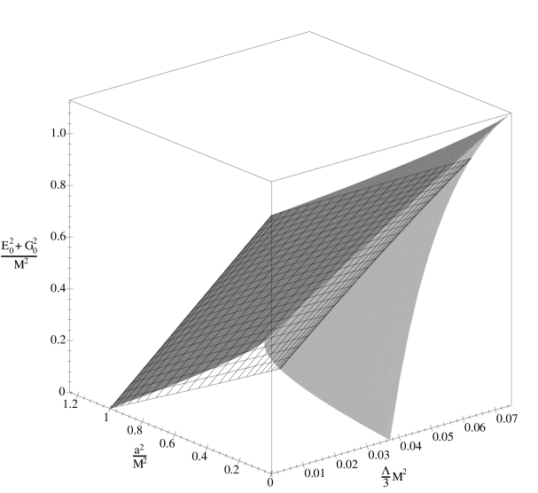
Figure 6.2: The allowed range of the KNdS parameters. The range is bounded by the planes $M=0$, $a^{2}=0$, $E_{0}^{2}+G_{0}^{2}=0$, the cold solutions (the darkest sheet) and the rotating Nariai solutions (the lighter gray sheet). Also shown as a meshed sheet are the lukewarm solutions.

Note that the extreme cases, though limits of the KNdS metric, have different global topological structures. In fact the Nariai and ultracold spacetimes do not even contain black holes. Their metrics in coordinate form may be found in appendix B.2, but here I’ll just comment briefly on some of their properties.

In the cold case the double horizon of the black hole recedes to an infinite proper distance from all other parts of the spacetime (as measured in a spacelike surface of constant $t$). Thus, the global structure of the spacetime changes. In particular, the region inside the black hole is cut off from the rest of the spacetime. Making appropriate periodic identifications of the global structure so that the spacetime contains two (in this case extreme) black holes, the structure is shown in figure 6.3. In that figure opposite sides of the rectangle are identified. $r=r_{c}$ is the cosmological horizon and $r=r_{o,i}$ is the double black hole horizon. If $a=0$, then the spacetime cuts off at the singularity at $r=0$. Otherwise, one may pass through the ring singularity to the negative values of $r$, including $r_{-}$, the fourth root of ${\mathcal{Q}}$. Note that in this case, the $t=\mbox{constant}$ hypersurfaces contain two extreme black holes, and so are not closed as they are in the regular KNdS spacetime. The metric for this case is given in appendix B.2.1.

Figure 6.3: The Penrose-Carter diagram for a two hole cold KNdS spacetime.

As noted the Nariai solution shown in 6.4 is no longer a black hole solution, and there is no longer a singularity at finite distance beyond either of the horizons at $\rho=\pm 1$. In fact, the diagram is the same as that for two-dimensional deSitter space. If there were no rotation ($a=0$), then this spacetime would just be the direct product of two-dimensional deSitter space, and a two-sphere of fixed radius. With rotation, of course the situation is not so simple but if $a=0$, it reduces to the non-rotating charged Nariai solution considered in [71]. The metric may be found in appendix B.2.2.

Figure 6.4: The Penrose-Carter diagram for the Nariai limit spacetime.

Even though the Nariai solution is not a black hole solution itself, it was shown in [43] that an uncharged, non-rotating Nariai solution is unstable with respect to quantum tunnelling into an almost-Nariai Schwarzschild-deSitter spacetime. It is usually argued [12] that this tunnelling carries over analogously with the inclusion of charge and rotation, in which case Nariai solutions decay into near Nariai KNdS spacetimes. Thus, in the future sections where I study black hole pair creation this solution will remain of interest, as a route to black hole pair creation will be to create a Nariai spacetime and then let it decay into a black hole pair.

A similar argument can be made [71] for the ultracold spacetimes found at the intersection of the parameter spaces of the cold and Nariai solutions. There are two possible spacetimes (appendix B.2.3), one with one horizon and the structure of Rindler space and the other which is conformally Minkowski and has no horizons. Neither contain black holes.

6.2.3 Issues of equilibrium

Before passing on to the next section where instantons to create the above spacetimes will be constructed, I’ll pause to examine whether these solutions to the Einstein-Maxwell equations are stable with respect to semi-classical effects. This is relevant because traditionally one only considered the quantum creation of black hole pairs in thermodynamic equilibrium, as it was thought that these were the only cases where regular instantons could be constructed. It is not so clear today (see for example [87, 47]) that that requirement must be enforced, but since I’ll be more-or-less using the traditional methods here and also try to draw some conclusions about the thermodynamics of the spacetimes, it is an issue that must be considered. To check for this equilibrium, one must consider three phenomena: thermodynamically driven particle exchange between the horizons, electromagnetic discharge of the holes (due to emission of charged particles), and spin-down of the holes (due to emission of spinning particles and super-radiance).

It is well known that a black hole emits particles in a black body thermal spectrum and thus may be viewed as having a definite temperature [48]. In the same way, it has been shown that deSitter horizons may also be viewed as black bodies and have a definite temperature [42]. For a spacetime with non-degenerate horizons, these temperatures may be most easily calculated by the conical singularity procedure [41] (which will show up again in the next section during the instanton construction). First, corotate the coordinate system with the horizon whose temperature is being calculated. Second, analytically continue the time coordinate to imaginary values. For definiteness label the imaginary time coordinate ${\mathcal{T}}$, the radial coordinate ${\mathcal{R}}$, and let the horizon be located at ${\mathcal{R}}={\mathcal{R}}_{h}$. Next, consider a curve in the ${\mathcal{T}}-{\mathcal{R}}$ plane with constant radial coordinate ${\mathcal{R}}={\mathcal{R}}_{0}$. Periodically identify the imaginary time coordinate with some period $P_{0}$ so that this curve becomes a coordinate “circle” and may be assigned a radius $R_{0}$ and circumference $C_{0}$ according to the integrals

$$R_{0}\equiv\left.\left(\int_{{\mathcal{R}}_{h}}^{{\mathcal{R}}_{0}}\sqrt{g_{{\mathcal{R}}{\mathcal{R}}}}d{\mathcal{R}}\right)\right|_{{\mathcal{T}}=0},\;\;\;\;\;\mbox{and}\;\;\;\;\;C_{0}\equiv\left.\left(\int_{0}^{P_{0}}\sqrt{g_{{\mathcal{T}}{\mathcal{T}}}}d{\mathcal{T}}\right)\right|_{{\mathcal{R}}={\mathcal{R}}_{0}}.$$ (6.11)

Finally, calculate $\lim_{{\mathcal{R}}_{0}\rightarrow{\mathcal{R}}_{h}}\frac{C_{0}}{R_{0}}$. Pick the value of $P_{0}$ so that the limit has value $2\pi$. Then, the horizon has temperature $T_{h}=1/P_{0}$, and surface gravity $\kappa_{h}=2\pi/P_{0}$.

If there is a degenerate horizon as is the case for a cold black hole, then that horizon is an infinite proper distance from all non-horizon points of the spacetime. In such a situation there is no restriction on the period with which the degenerate horizon can be identified, and it has been argued [49] that the black hole can therefore be in equilibrium with thermal radiation of any temperature.

Now consider which of the spacetimes are in thermodynamic equilibrium. First, consider the general non-extreme KNdS solutions. The temperature of the outer black hole horizon and the cosmological horizon are respectively,

$$T_{bh}=\left.\left(\frac{1}{4\pi\chi^{2}(r^{2}+a^{2})}\frac{d{\mathcal{Q}}}{dr}\right)\right|_{r=r_{bh}}\;\;\;\mbox{and}\;\;\;T_{ch}=\left.\left(\frac{-1}{4\pi\chi^{2}(r^{2}+a^{2})}\frac{d{\mathcal{Q}}}{dr}\right)\right|_{r=r_{ch}}$$ (6.12)

There are two ways that these two temperatures may be equal. The first is if $r_{bh}=r_{ch}$ which actually is the Nariai spacetime. However there is also a non-extreme solution labelled the lukewarm case. Its parameterization is considered in appendix B.2.4.

The cold limit is in thermodynamic equilibrium at the temperature of the cosmological horizon, for as has been noted an extreme black hole may be in equilibrium with thermal radiation of any temperature. As noted, the Nariai limit too is in thermodynamic equilibrium, with both horizons having the same temperature

$$T_{Nar}=\frac{\frac{\Lambda}{3}(4e^{2}-\delta^{2})}{4\pi},$$ (6.13)

where $e$ and $\delta$ are defined in appendix B.2.2. The first ultracold case has only one horizon with temperature

$$T_{UCI}=\frac{1}{2\pi},$$ (6.14)

and so with no other horizon to balance this one off, it is not in thermal equilibrium. The second ultracold case has no horizons, and so is trivially in equilibrium.

Next consider discharge of the black holes. Even if the black hole and cosmological horizon are in equilibrium with respect to thermal particle exchange between them, there can still be a net exchange of charge between the horizons. The mechanism is that even though both may create the same number and masses of particles, an excess of charged particles will be created at the black hole horizon, and so it will discharge [40]. This effect can be quite rapid and so in most cases a charged black hole cannot be said to be truly in equilibrium. However, there are a couple of ways to avoid the discharge. If there are no particles of the appropriate charge that are also lighter than the black hole then discharge cannot occur. Thus, if magnetic monopoles do not exist then the magnetic holes will be stable with respect to discharge. Further, even if the appropriate light charged particles exist, the discharge effects will be small if the temperature of the black hole is small relative to the mass of those particles. That is, the more massive the black hole, the slower the discharge.

Finally consider the spin-down of the black holes. If the black holes and cosmological horizons are at the same temperature, then there will be no net energy exchange between the horizons, but the particles created at the black hole horizons may still have an excess of angular momentum relative to those created at the cosmological horizons. Unfortunately this effect is not as well studied for cosmological spacetimes as is the equivalent discharge case. Still, from the extensive calculations in asymptotically flat space [77, 76, 24] one can say the following. In flat space, the direct spin-down by particle creation is a relatively slow process but it is greatly amplified by super-radiance. In combination the two processes cause angular momentum to be radiated relatively more quickly than mass is radiated unless there are a truly ridiculous number of scalar fields in the spacetime [24]. Preliminary indications [83] are that spin-down occurs at least as quickly and possibly more quickly in asymptotically deSitter spacetimes which are not in thermal equilibrium. There aren’t any corresponding calculations for black holes which are in thermal equilibrium with cosmological horizons, but that said, in the other cases spin-down is a relatively quick effect which means that a rotating black hole in deSitter space probably cannot be thought of as being in full equilibrium. Possibly the presence of thermal equilibrium might cause something miraculous to happen, but that is unlikely and in any case a matter to be resolved by future calculations. However, even in the absence of such a miracle, the physically intuitive notion that a black hole that is rotating slowly relative to its mass will discharge slowly is supported by the existing results, and so it seems likely that at least a class of these holes may be considered quasi-static in a thermodynamic sense.

That said, in the following section I’ll show that only thermal rather than full thermodynamic equilibrium appears to be required for the construction of smooth instantons. Of course if the created system is not in full equilibrium one cannot really draw conclusions about its thermodynamics. Thus, the reader who is uncomfortable with the quantum creation of spacetimes that are not in full thermodynamic equilibrium can consider all of the following to apply only to the subset of spacetimes that are at least quasi-static.

6.3 Instanton assembly

In this section I construct the instantons that will be used to study the creation of the spacetimes considered in the previous section. As discussed in the review of the path integral formalism, these instantons must both be solutions to the Einstein-Maxwell equations and also should match as smoothly as possible along a spacelike hypersurface onto the spacetime that they create. The instantons constructed here will satisfy the cosmological no boundary condition, and so I will not need to worry about matching to initial conditions.

6.3.1 Analytic continuation

For static spacetimes, the first step of instanton construction is usually to analytically continue $t\rightarrow i\tau$. For a static spacetime expressed in appropriate coordinates, this gives a real Euclidean solution to the equations of motion but for a spacetime that is only stationary it will usually produce a complex solution to the equations of motion. For now I accept this complex solution but at the end of this section I’ll consider its relative merits compared to the more standard approach where other metric parameters are also analytically continued in order to obtain a real Euclidean metric. That said, I proceed in the following manner (which is equivalent to continuing $t\rightarrow i\tau$).

If a spacetime is foliated by a set of space-like hypersurfaces $\Sigma_{t}$ labelled by a time coordinate $t$, the most general Lorentzian metric can be written as

$$ds^{2} = -N^{2}dt^{2}+h_{ab}(dx^{a}+V^{a}dt)(dx^{b}+V^{b}dt)$$

$$= (-N^{2}+h_{ab}V^{a}V^{b})dt^{2}+2h_{ab}V^{b}dx^{a}dt+h_{ab}dx^{a}dx^{b},$$

where as usual $h_{ab}$ is the induced metric on the hypersurfaces, $N$ is the lapse function, and $V^{a}$ is the shift vector field. Using the prescription of [17], the analytic continuation can be made by making all of the Lagrange multipliers from the Hamiltonian purely imaginary. To wit, I start by changing the lapse and shift so that $N\rightarrow iN$ and $V^{a}\rightarrow iV^{\alpha}$. The spacetime metric for the proto-instanton then becomes

$$ds^{2}=(N^{2}-h_{ab}V^{a}V^{b})dt^{2}+2ih_{ab}V^{b}dx^{a}dt+h_{ab}dx^{a}dx^{b}.$$ (6.16)

If $V^{i}=0$ then this metric has a Euclidean signature, whereas if $V^{i}\neq 0$ then the metric is complex and its signature is not so easily defined. There is a sense however in which it is still Euclidean. At any point $x_{0}^{\alpha}$ one can make a complex coordinate transformation $x^{a}=\tilde{x}^{a}-it\left.V^{a}\right|_{x_{0}}$ (or equivalently add a complex constant to the shift), to obtain the metric

$$\left.ds^{2}\right|_{x^{a}_{0}}=N^{2}dt^{2}+h_{ij}dx^{i}dx^{j},$$ (6.17)

at $x^{a}_{0}$. Thus the signature is Euclidean at any point modulo a complex coordinate transformation. Following the Lagrange multiplier prescription, the electromagnetic field is made complex by rotating the Coulomb potential $\Phi\rightarrow i\Phi$ which changes the Maxwell field tensor as

$$F_{ta}\rightarrow iF_{ta},\;\;F_{at}\rightarrow iF_{at},\ \ \mbox{and}\ F_{ab}\rightarrow F_{ab},$$ (6.18)

where as usual the Latin indices indicate a restriction to the spatial slices. If the original Lorentzian metric and electromagnetic field were solutions to the Einstein-Maxwell equations, then so are this complex metric and electromagnetic field.

I now show that this complex solution can be matched onto the real solution from which it was derived.

6.3.2 Matching the complex to the Lorentzian

The obvious hypersurface along which to match the Lorentzian solution to its complex “Euclidean” counterpart described above, is a hypersurface of constant $t$. I specialize the general metric (6.3.1) to the stationary, axisymmetric case where $x^{1}=\phi$, $x^{2}=\theta$, and $x^{3}=r$. Then, $V^{a}=[V^{\phi}(r,\theta),0,0]$, $N=N(r,\theta)$, and $h_{ab}=\mbox{diag}[h_{\phi\phi}(r,\theta),h_{\theta\theta}(r,\theta),h_{rr}(r,\theta)]$. This specialization will remain general enough to cover the cases of interest in this thesis.

Now, consider how the complexified solution does or does not match onto the Lorentzian solutions across a surface of constant $t$. First, the unit normal to $\Sigma_{t}$ is $u_{\alpha}=\pm N[dt]_{\alpha}$ where $[dt]_{\alpha}$ is the coordinate version of $dt$. Choosing it to be forward pointing on the Lorentzian side and consistently oriented on the “Euclidean” side $u_{\alpha}=-N[dt]_{\alpha}$ in each case. Then, on the Lorentzian side the induced metric is $h_{ab}=g_{ab}+u_{a}u_{b}$ while on the “Euclidean” side it is $\tilde{h}_{ab}=g_{ab}-u_{a}u_{b}$ which are both equal to $\mbox{diag}[h_{\phi\phi},h_{\theta\theta},h_{rr}]$. Thus, the induced hypersurface metrics match and so a geometrical matching is possible. In the same way, the same vector potential $\tilde{A}_{a}$ is induced from both sides, so from a purely Hamiltonian point of view, the configuration variables match.

Of course for the matching to be smooth, both sides should also induce the same extrinsic curvature on the surface (as discussed by Israel in [59] and already discussed for timelike surfaces in section 3.6 of this thesis). Unfortunately with $u_{\alpha}$ as defined above, the extrinsic curvatures $K_{ab}=e_{a}^{\alpha}e_{b}^{\beta}\nabla_{\alpha}u_{\beta}$ are not the same. Namely on the Lorentzian side,

$$K_{ab}\equiv e_{a}^{\alpha}e_{b}^{\beta}u_{{\alpha};{\beta}}=\left[\begin{array}[]{ccc}0&\frac{h_{\phi\phi}\partial_{\theta}V^{\phi}}{2N}&\frac{h_{\phi\phi}\partial_{r}V^{\phi}}{2N}\\ \frac{h_{\phi\phi}\partial_{\theta}V^{\phi}}{2N}&0&0\\ \frac{h_{\phi\phi}\partial_{r}V^{\phi}}{2N}&0&0\end{array}\right],$$ (6.19)

while on the “Euclidean” side the extrinsic curvature is $iK_{ab}$. In a similar way, the induced electric field on the “Euclidean” side is $iE_{a}$ where $E_{a}$ is the Lorentzian field.

Then, from the Hamiltonian perspective adopted in this thesis the situation is as follows. Configuration variables $h_{ab}$ and $\tilde{A}_{a}$ remain real under the complex transformation, while their conjugate momenta $P^{ab}=\sqrt{h}/(2\kappa)(Kh^{ab}-K^{ab})$ and ${\mathcal{E}}^{a}=-2\sqrt{h}/\kappa E^{a}$ become purely imaginary along with the Lagrange multipliers. Thus a matching is possible, though it isn’t smooth.

The conclusions of section 3.6 for spacetimes where there is an extrinsic curvature discontinuity across a timelike hypersurface apply equally well in this section where the discontinuity is across a spacelike surface. That is, the discontinuity corresponds to a thin shell of matter. In this case the stress-energy tensor representing the matter is imaginary and since it is spacelike exists only instantaneously. This is unusual to say the very least, but then again the surface $\Sigma_{t}$ separates regions with different metric signature so perhaps it isn’t surprising that something strange might occur at that surface. What is more of a concern however is that the presence of this strange matter at the borders of the instanton might shift the action of the solution away from extremality. If that is the case then the instanton cannot be used to approximate the full path integral. This matter deserves further investigation, though I will not do that here.

In section 6.4, where I select an appropriate action for evaluating the path integral, it will be seen that this situation of real and complex fields actually integrates quite nicely into the path integral formalism, but at first glance the discontinuities are a bit disturbing. It is clear however, that the complications have arisen from the inclusion of rotation. In earlier pair creation studies (such as [30, 29, 39, 49, 71, 23, 69, 70, 12]) there was no rotation which meant $K_{ab}=0$ and the geometric matching was smooth. The discontinuity in the electric field remained, though it wasn’t usually considered.

Before moving on, I’ll point out that by the traditional methods of instanton construction such as those used in [73, 64, 86] the situation would be even worse. The standard method would require that I analytically continue as many parameters of the metric as necessary to arrive at a real and Euclidean solution to the Einstein-Maxwell equations. For example, with the Kerr-Newman-deSitter solutions, which will soon be under consideration, the rotation and electric charge parameters would be made complex ($a\rightarrow ia$, $E_{0}\rightarrow iE_{0}$) so that the Euclidean metric and electric field would be real. Although this approach avoids dealing with complex metrics, it incurs several serious problems of its own. Specifically, sending $a\rightarrow ia$ and $E_{0}\rightarrow iE_{0}$ means that the surface metric $h_{ab}$ itself is affected by the transformation. In detail, the polynomial ${\mathcal{Q}}$, and functions ${\mathcal{G}}$ and ${\mathcal{H}}$ (defined in and before equation (6.2.1)) are all changed and so $h_{rr}\neq\tilde{h}_{rr}$, $h_{\theta\theta}\neq\tilde{h}_{\theta\theta}$, and $h_{\phi\phi}\neq\tilde{h}_{\phi\phi}$. That this is not just a problem of coordinates is made clear most dramatically by the fact that the change in ${\mathcal{Q}}\rightarrow-\frac{\Lambda}{3}r^{4}+(1+\frac{\Lambda}{3}\tilde{a}^{2})r^{2}-2Mr-\tilde{E_{0}}^{2}+G_{0}^{2}$ will certainly shift, and often entirely change its number of roots, which means that the “horizon” structure of the spatial surface will be different on each side of $\Sigma_{t}$. Thus, by the traditional method the “Euclidean” solution emphatically would not match onto the Lorentzian solution.

Given that the matching conditions are the only existing prescription that definitively link instantons with physical Lorentzian solutions, I choose to keep what matching conditions I can, abandon the requirement that the full spacetime metric be real, and proceed with the calculation.

6.3.3 Putting the parts together

With these general steps taken, I’m now ready to finish off the instantons. They will come in three classes: i) those creating spacetimes with two non-degenerate horizons bounding the primary Lorentzian sector (this case will create Nariai and lukewarm spacetimes), ii) those creating spacetimes with only a single non-degenerate horizon bounding the Lorentzian sector, (this case will create cold spacetimes and ultracold I spacetimes), and iii) and those creating zero horizon spacetimes (here, the ultracold II spacetime).

Spacetimes with two nondegenerate horizons

By the procedure described above I have found a complex solution that may be joined to the Lorentzian solution from which it was generated. However a subtlety arises in that the constant $t$ spatial hypersurfaces of the nondegenerate KNdS and Nariai spacetimes both consist of two Lorentzian regions that are connected to each other across their corresponding horizons, while the constant $t$ hypersurfaces of the complex solution consist of only one such region. The complex solution may be connected to both sections simultaneously by the following procedure (that is illustrated in figure 6.5).

Figure 6.5: Construction of a two-horizon instanton. The radial/time sector is shown. The heavily dashed lines indicate that the solution continues in that direction.

First, connect half of a full Lorentzian solution (the region bounded by the outer black hole and cosmological horizons) to each of the $t=0$ and $t=\frac{P_{0}}{2}$ hypersurfaces of the “Euclidean” solution (as in figure 6.5a). Next (figure 6.5b) fold the construction over, and identify outer horizon to outer horizon, and inner horizon to inner horizon (figure 6.5c). The $t=\mbox{constant}$ hypersurfaces of the Lorentzian part of the construction now consist of two regions with opposite spin and charge, and are the complete $t=\mbox{constant}$ hypersurfaces of the maximally extended but periodically identified KNdS solutions that I considered earlier.

Next note that the metric at any point of the Riemannian part of the construction is

$$ds^{2}=N^{2}dt^{2}+h_{ij}dx^{i}dx^{j}$$ (6.20)

under the coordinate transformation that eliminates the shift at that point. At the horizons $N^{2}\rightarrow 0$ for these solutions. Therefore it is reasonable to identify the entire time coordinate along the horizons as a single time (figure 6.5d). The instanton is nearly complete. The “Euclidean” part is smooth everywhere except at the points where I made the identification and probably introduced conical singularities.

Now, for a given horizon at $r=r_{h}$, I can find a period $P_{0}$ such that $\lim_{r\rightarrow r_{h}}\frac{P_{0}\partial_{r}\tilde{N}}{\sqrt{h_{rr}}}=2\pi$ which in turn implies that the conical singularity has been eliminated. This is the same condition used in calculating the temperature of the horizons in section 6.2.3, and so those results may be reused here. Hence the only double-horizon cases where the conical singularities at the two horizons may be simultaneously eliminated (figure 6.5e) and so the only cases where the instanton will everywhere be a solution to the Einstein equations, are the lukewarm and Nariai instantons, for which

$$P_{0}^{lw}=\frac{4\pi\chi^{2}(r_{bh}^{2}+a^{2})}{Q^{\prime}(r_{h})}\ \mbox{and}\ \ P_{0}^{Nar}=\frac{4\pi}{\frac{\Lambda}{3}(4e^{2}-\delta^{2})}$$ (6.21)

respectively. $Q^{\prime}=\frac{dQ}{dr}$, and $r_{bh}$ is the radius of the outer black hole horizon in the lukewarm solution. Then, the full construction of Lorentzian and Euclidean parts is smooth everywhere, except on the $\Sigma_{t}$ transition surface where there will be a mild jump discontinuity in the extrinsic curvatures.

Next consider the single-horizon spacetimes.

Spacetimes with one non-degenerate horizon

It is now fairly easy to build the single non-degenerate horizon instantons for the cold and ultracold I spacetimes (even though the cold spacetime has two horizons, the inner horizon is a degenerate, double horizon). For these spacetimes, attach half-copies of the Lorentzian spacetime at the $t=0$ and $t=\frac{P_{0}}{2}$ hypersurfaces of the complex Riemannian section (figure 6.6a). Then fold and identify the cosmological horizons to reconstruct the full Lorentzian $t=\mbox{constant}$ hypersurfaces (figure 6.6b and c). Next, identify the time coordinate along the cosmological horizon (figure 6.6d). Finally, with just one horizon choose

$$P_{0}^{cold}=-\frac{4\pi\chi^{2}(r_{ch}^{2}+a^{2})}{Q^{\prime}(r_{ch})}\qquad\mbox{ and}\qquad P_{0}^{UCII}=2\pi,$$ (6.22)

where $Q^{\prime}(r_{ch})=\left.\frac{dQ}{dr}\right|_{r=r_{ch}}$ and $r_{ch}$ is the radius of the cosmological horizon. Then the instanton will have no conical singularities (figure 6.6e).

Figure 6.6: Construction of a one-horizon instanton. The radial/time sector is shown. The heavily dashed lines indicate that the solution continues in that direction.

No-horizon spacetimes

This time the construction is less definite. With no identifications being made, and no horizons to define a period, the instanton has indefinite period creating two disjoint spacetimes (figure 6.7). This corresponds to the ultracold II case.

Figure 6.7: Construction of a no-horizon instanton. The radial/time sector is shown. The heavily dashed lines indicate that the solution continues in that direction.

6.4 Choosing an appropriate action

As was discussed in chapters 3 and 4, if one chooses a Lagrangian action $I$, takes its first variation $\delta I$ over a finite region $M$, and solves $\delta I=0$, then the solution includes not only field equations in the bulk, but also boundary conditions on the fields over $\partial M$. Thus in choosing an action that is appropriate to a particular situation, one must keep in mind the implied boundary conditions that are attendant upon it.

In particular, in the path integral formulation of gravity for finite regions of spacetime, the action choice also fixes boundary conditions that the possible paths must satisfy, and therefore restricts the allowed parameter space of those paths. There are two ways of approaching the choice of how the parameter space should be restricted. The first is from a geometrical/topological point of view. There one considers what geometrical properties the paths should have so that they will properly match onto the Lorentzian solutions. The second way is much more physical and considers what physical restrictions should be placed on the paths so that they will produce the types of spacetime that one is interested in. That is, one demands that the created spacetime has certain physical characteristics such as horizons, temperatures of those horizons, and a particular angular momentum or electric/magnetic charge and then enforces those same restrictions on the “paths” so that they will create the correct spacetimes. Happily, as will be seen below, these apparently disparate approaches complement each other and produce compatible lists of restrictions.

First from a geometrical point of view, it is essential that the “paths” match, onto the Lorentzian solution along the interface surface $\Sigma_{2}$. That is, they should all induce the correct surface metric $h_{ab}$ and vector potential $\tilde{A}_{a}$ on $\Sigma_{2}$. Examining the Hamilton-Jacobi variation (3.2.2) (the orthogonal version is sufficient in this case) it is clear that the standard action functional has this property. Note however that the formalism does not guarantee that the conjugate momenta $P^{ab}$ (or equivalently the extrinsic curvatures) and ${\mathcal{E}}^{a}$ will match as well. In an ideal world both would be fixed but since they are conjugate to each other this is not possible. Given this and the fact that the instanton work showed that for that solution the conjugate momenta don’t in fact match across the transition surface, I’ll fix the configuration variables and leave the other two free.

Continuing with the geometry recall the conditions that were placed on the instantons. Namely I required that they have only one boundary ($\Sigma_{2}$ that matches onto the Lorentzian solutions) and further that they be smooth and without conical singularities. That is I demanded that $N=0$ (because the foliation of the spacetime is othogonal to the boundary in this case, I’ll drop the bar notation) at the coordinates values of $r$ corresponding to non-degenerate horizons in the Lorentzian solution and further that

$$\lim_{r\rightarrow r_{h}}\frac{\int_{0}^{P_{0}/2}dtN}{\int_{r_{h}}^{r}dr\sqrt{h_{rr}}}=\lim_{r\rightarrow r_{h}}\frac{P_{0}\partial rN}{2\sqrt{h_{rr}}}=\pi,$$ (6.23)

where $r_{h}$ is the coordinate of the horizon. At first glance that second condition appears to be awkward and abstruse but in fact it is quite straightforward to show that if $N=0$ at $r_{h}$ then

$$\lim_{r\rightarrow r_{h}}Np=\frac{2}{\kappa}n^{a}\partial_{a}N,$$ (6.24)

where $p$ is the pressure defined at the end of section 3.4. Now $n^{a}=\frac{1}{\sqrt{h}}\partial^{a}_{r}$ and so to avoid conical singularities one must fix $Np$. To ensure this, it is more than sufficient to fix $Ns^{ab}$. Turning again to the action variation (3.2.2) the reader will note that $N$ is already fixed while $Ns^{ab}$ has been left free. Adding

$$\Delta I_{p} \equiv -\frac{1}{2}\int dt\int_{\Omega_{t}}d^{2}x\sqrt{\sigma}Np,$$ (6.25)

to the action the situation is corrected and one can force the paths to be closed and smooth at the points corresponding to non-degenerate horizons.

There is also a nice physical interpretation of these conditions. Namely fixing the lapse $N$ to be zero at $r_{h}$ means that there will be an (apparent) horizon at that point while putting the restrictions on $Np$ fixes the temperature of those horizons (see section 6.2.3). Therefore enforcing these conditions at $r_{h}$ means that there will be a horizon of predetermined temperature there. If there are two non-degenerate horizons then each will have a temperature. By the no-conical-singularity requirement of geometrical smoothness, they must have the same temperature and so geometrical smoothness is equivalent to the thermal equilibrium of the final state.

Next consider what should be done at a degenerate horizon such as that found in a cold spacetime and what restrictions should be placed on the “paths” that might create it. To match onto the Lorentzian solution all paths must have the “tapered horn” shape characterized by $N\rightarrow 0$ at the degenerate horizon. Since the horizon is an infinite proper distance from the rest of the spacetime, there is no need to worry about conical singularities, and therefore no need to fix the pressure. Instead leave $\sigma_{ab}$ fixed to ensure that the metric will have the correct asymptotic behaviour. Thus at degenerate horizons do not add $\Delta I_{p}$ to the action. Note that this geometrical behaviour is the basis of the claim [49] that an extreme black hole doesn’t have a fixed temperature but instead can be in thermodynamic equilibrium with any background.

Having set the boundary conditions to ensure that the spacetimes contain black holes it is natural to fix the angular momentum and electromagnetic charge of those black holes. Afterall the ultimate intention is to calculate the pair creation rates for pairs of black holes of specified mass, angular momentum, and charge so these quantities must be fixed in advance or else the path integral will calculate the creation rate for some other situation. At first it might seem natural to fix ${\varepsilon}$ as well so that one could specify the mass of the holes being created but as was noted above one can fix $N$ or ${\varepsilon}$ but not both. $N$ must be fixed so that the black holes can be guaranteed to exist, so ${\varepsilon}$ has to be left free. That said, to fix the angular momentum one must add

$$\Delta I_{j}\equiv-\int dt\int_{\Omega_{t}}d^{2}x\sqrt{\sigma}V^{a}j_{a},$$ (6.26)

to the action.

Next consider fixing the electromagnetic charges. First recall from chapter 4, that by choosing to work with $I_{m}$, $F_{{\alpha}{\beta}}$, and $A_{\alpha}$ I have automatically excluded magnetically charged solutions from consideration. At the same time however, the electric charge has been left free (see the variation (4.2.2)). By the previous paragraph it should be fixed and so add

$$\Delta I_{el}\equiv\frac{1}{\kappa}\int dt\int_{\Omega_{t}}d^{2}xN\sqrt{\sigma}n_{\alpha}F^{{\alpha}{\beta}}A_{\beta},$$ (6.27)

to the action. There is a choice of whether to fix ${\mathcal{E}}^{a}$ or $\tilde{A}_{a}$ on the boundary $\Sigma_{2}$. As has already been noted $\tilde{A}_{a}$ is the appropriate quantity to fix and that doesn’t require an extra boundary term on $\Sigma_{2}$.

By contrast if I want to consider magnetic black holes I use $I_{m}^{\star}$, $\star F_{{\alpha}{\beta}}$, and $A^{\star}_{\alpha}$. Then electric charges are automatically eliminated from consideration and

$$\Delta I^{\star}_{mg}\equiv\frac{1}{\kappa}\int dt\int_{\Omega_{t}}d^{2}xN\sqrt{\sigma}n_{\alpha}\star\!F^{{\alpha}{\beta}}A^{\star}_{\beta},$$ (6.28)

should be added to the action to fix the created magnetic charges. No additional boundary term is required to fix $\tilde{A}^{\star}_{a}$ on $\Sigma_{2}$.

Switching to the thermodynamic interpretation of the path integrals it is immediate that what is being considered here is a canonical partition function. That is, extensive variables (angular momentum and electric/magnetic charge) are fixed except for the energy which is left free in favour of holding the temperature constant. This is then in accord with the standard approach to pair creation calculations which uses that partition function [52]. This choice then ensures that created spacetimes are in thermal equilibrium, that there is no discontinuity in physical properties such as electromagnetic charge and angular momenta at the juncture of the paths and the Lorentzian solution, and from a geometric point of view that the paths are smooth and match onto the Lorentzian solution.

6.5 Evaluating the actions - pair creation rates and entropy

As noted earlier, creation rates for these spacetimes are proportional to $e^{-2I_{inst}}$, where $I_{inst}$ is the numerical value of the action of the appropriate instanton. Now, as was laid out in section 6.1, those rates are calculated only up to a normalization factor. Evaluating this normalization factor would involve fully evaluating another ill-defined path integral so I will side-step that issue by calculating the probability of creation of these spacetimes relative to deSitter space. Then the normalization factors cancel each other out and the relative probability of creation of the black holes in a deSitter background is

$$P=\exp{(2I_{dS}-2I)},$$ (6.29)

where $I$ is the action of the instanton, and $I_{dS}$ is the action of an instanton mediating the creation of deSitter space with the same cosmological constant. Conventionally, this probability is also interpreted as the probability that deSitter space will tunnel into a given black hole spacetime [13].

A further link to thermodynamics is found by the following argument. The spacelike hypersurfaces of the spacetimes that I have considered are all topologically closed and with finite volume. Then, the energy is trapped in the hypersurfaces and so they can be interpreted as having constant energy even though that condition has not been enforced by boundary conditions [71, 52]. By that reasoning the canonical partition function is equivalent to the microcanonical partition function in this case, and so as is standard for a microcanonical partition function, the entropy of the created spacetime is

$$S=\ln{\Psi^{2}}=-2I.$$ (6.30)

Thus, at least in the case where the created spacetime is quasi-static, there is a close connection between pair creation rates and the entropy of the spacetimes and in particular it is consistent with the idea that the entropy is the logarithm of the number of quantum states. With all of this in mind I evaluate the appropriate action for each spacetime.

Momentarily leaving aside the matter terms, the appropriate action by all of the above considerations is

$$I_{(N,p,j)} = I+\Sigma_{SH}\Delta I_{p}+\Sigma_{AH}\Delta I_{j}$$ (6.31)

$$= \left(\mbox{ terms that vanish for stationary solutions }\right)$$

$$+\Sigma_{AH}\int_{B_{h}}d^{3}x\sqrt{\sigma}N\varepsilon-\frac{1}{2}\Sigma_{SH}\int_{B_{h}}d^{3}x\sqrt{\sigma}Np,$$

where the subscript $SH$ indicates a sum over all single, non-degenerate horizons and $AH$ means a sum over all horizons regardless of their degeneracy. Keeping in mind that $N=0$ on all of the horizons, it is clear that the $N\varepsilon$ terms are zero. Further, recall equation (6.24) which says $Np=(2/\kappa)n^{a}\partial_{a}N$ and equation (6.23) which implies that $n^{a}\partial_{a}N=(2\pi)/P_{0}$ on a non-degenerate horizon. Then

$$I_{(N,p,j)}=-\Sigma_{SH}\frac{{\mathcal{A}}_{H}}{8},$$ (6.32)

where ${\mathcal{A}}_{H}$ is the surface area of the event horizons in the spatial surface $\Sigma_{2}$.

Next, consider the matter terms. For electric solutions it is a trivial use of Stokes’s theorem to show that,

$$-\frac{1}{2\kappa}\int_{M}d^{4}x\sqrt{-g}(F_{{\alpha}{\beta}}F^{{\alpha}{\beta}})+\Delta I_{el}$$ (6.33)

$$= \int_{M}d^{4}x\sqrt{-g}(A_{\beta}\nabla_{\alpha}F^{{\alpha}{\beta}})-\frac{1}{\kappa}\int_{\Sigma}d^{3}x\sqrt{h}E^{a}\tilde{A}_{a}.$$

Of course the first term includes the constraint equation (2.12) and so is zero for solutions to the Maxwell equations. Thus all that is left is the second term, but it too is zero for the solutions in which I’m interested, and so the total electric term is also zero. Thus, the value of the action that keeps $N$, $p$ (if appropriate), $j_{a}$, and $E_{0}$ fixed (and $G_{0}=0$) is

$$I_{(N,p,j,E_{0})}=-\Sigma_{SH}\frac{{\mathcal{A}}_{H}}{8}.$$ (6.34)

The same line of reasoning shows that the value of the action that keeps $N$, $p$ (if appropriate), $j_{a}$, $G_{0}$ fixed (and $E_{0}=0$) is

$$I^{\star}_{(N,p,j,G_{0})}=-\Sigma_{SH}\frac{{\mathcal{A}}_{H}}{8}.$$ (6.35)

Assuming that the spacetimes are at least quasi-static, then equation (6.30) says that the entropy of these spacetimes is equal to one-quarter of the sum of the areas of non-degenerate horizons bounding the Lorentzian region of the spacetime. Consistent with references [49] and [71], the degenerate horizon in the cold case does not contribute to the entropy of the cold spacetime.

Using these general formulae for the pair creation rates and entropy of the spacetimes, I now consider each of the specific spacetimes separately.

The lukewarm action: In this case, there are non-degenerate cosmological and outer black hole horizons. Therefore the numerical value of the action of the electric/magnetic instantons is

$$I_{LW}=-\frac{{\mathcal{A}}_{c}+{\mathcal{A}}_{h}}{8}=-\frac{\pi(r_{c}^{2}+a^{2})}{2\chi^{2}}-\frac{\pi(r_{h}^{2}+a^{2})}{2\chi^{2}},$$ (6.36)

where ${\mathcal{A}}_{c}$ and ${\mathcal{A}}_{h}$ are respectively the areas of the cosmological and outer black hole horizons at $r_{c}$ and $r_{h}$ in the Lorentzian solution.

The Nariai action: Again there are two non-degenerate horizons, this time at $\rho=\pm 1$. Therefore the total action of the electric/magnetic Nariai instantons is

$$I_{N}=-\frac{{\mathcal{A}}_{\rho=-1}+{\mathcal{A}}_{\rho=1}}{8}=-\frac{\pi(e^{2}+a^{2})}{\chi^{2}},$$ (6.37)

where ${\mathcal{A}}_{\rho=\pm 1}$ is the area of the horizon at $\rho=\pm 1$. Note that for the Nariai solutions ${\mathcal{A}}_{\rho=1}={\mathcal{A}}_{\rho=-1}$.

The cold action: Here there is only one non-degenerate horizon, and so

$$I_{C}=-\frac{{\mathcal{A}}_{c}}{8}=-\frac{\pi(r_{c}^{2}+a^{2})}{2\chi^{2}},$$ (6.38)

where ${\mathcal{A}}_{c}$ is again the area of the cosmological horizon at $r_{c}$.

The ultracold I actions: Again there is only a single nondegenerate horizon, this time at $R=0$. The action of the magnetic ultracold I instanton is then

$$I_{UCI}=-\frac{{\mathcal{A}}_{0}}{8}=-\frac{\pi(e^{2}+a^{2})}{2\chi^{2}}.$$ (6.39)

where ${\mathcal{A}}_{0}$ is the area of the Rindler horizon as $R=0$.

Ultracold II Actions: There are no horizons whatsoever for this case, and so

$$I_{UCII}=0,$$ (6.40)

irrespective of the chosen period $P_{0}$ of the time coordinate, which is good since as was seen in section 6.3, that period is not specified by the formalism!

In figure 6.8, I plot these actions as a fraction of the action of the instanton creating deSitter space with the same cosmological constant. The instantons/created spacetimes are parameterized by $\frac{a^{2}}{M^{2}}$ and $\frac{\Lambda}{3}M^{2}$. For all cases $I,I_{dS}<0$ and from the diagram it is clear that $|I|<|I_{dS}|$. Then $I_{dS}-I<0$ and so each of the spacetimes considered above is less likely to be created than pure deSitter space with the same cosmological constant. Note that the Nariai spacetime is the most likely to be created provided the parameter values are such that the instanton exists, while the cold spacetime is the least likely to be created. As might expected on physical grounds, smaller and more slowly rotating holes are more likely to be created than larger and more quickly rotating ones. As $\frac{a}{M}\rightarrow 0$ and $M\rightarrow 0$, the creation rates approach those of deSitter space which again is physically reasonable.

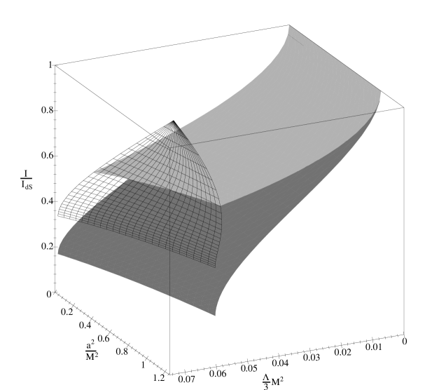
Figure 6.8: The actions for the charged and rotating lukewarm, cold, and Nariai instantons plotted as a fraction of the action of deSitter space with the same cosmological constant. The Nariai instantons are the meshed sheet, the lukewarm instantons are the lighter grey sheet, and the cold instantons are the darker grey sheet.The ultracold I instanton actions may be found at the “bottom” end of the cold sheet, while the ultracold II instanton actions are zero.

6.6 Reflections on the calculation

The approach to pair creation taken here is a bit different from that taken in most of the literature and because rotation has been included new issues have arisen that were not present in those papers. Thus in this section I will compare the methods and examine those issues a little further.

First I will compare the way I calculated actions here with the way it was done in reference [71] (which is representative of the more traditional calculations done for non-rotating black holes). There, the fact that the instantons are closed and smooth at the points corresponding to the non-degenerate horizons was taken to mean that no boundary terms need be considered there, implying that the basic action used for the lukewarm and Nariai instanton should be

$$I_{old}=-\frac{1}{2\kappa}\int_{M}d^{4}x\sqrt{-g}\left({\mathcal{R}}-2\Lambda-F^{2}\right)-\frac{1}{\kappa}\int_{\Sigma}d^{3}x\sqrt{h}K,$$ (6.41)

which from my point of view is the Lagrangian action (4.1) with the boundary term

$$\frac{1}{\kappa}\int_{B}d^{3}x\sqrt{-\gamma}\Theta$$ (6.42)

added on. It is easy to see that this term is equivalent to the pressure term

$$-\int_{B}d^{3}xN\sqrt{\sigma}\frac{p}{2}=-\int_{B}d^{3}xN\sqrt{\sigma}\left[\frac{n^{a}\partial_{a}N}{N}-\frac{k}{2}\right],$$ (6.43)

evaluated on the equivalent horizons. To see this, note that $\Theta=k-\frac{n^{a}\partial_{a}N}{N}$, $k=-\frac{1}{2\sqrt{h_{rr}}}\partial_{r}\ln\sigma$, and $\frac{1}{\sqrt{h_{rr}}}\rightarrow 0$ at each horizon. So on those horizons $\Theta=-\frac{p}{2}$ and in the absence of rotation my approach is equivalent to that of [71].

For the cold case, $k$ still vanishes on the boundary and so the inclusion of the $\Theta$ term in [71] is equivalent to the omission of the pressure term in my calculation. Finally, in the ultracold cases $k=0$ everywhere and so once more the omissions/inclusions are equivalent.

For electric instantons in both calculations, electromagnetic boundary terms are added to the action to fix the electric charge for all paths considered in the path integral. Further, in both calculations for solutions to the Maxwell equations, these boundary terms may be converted into the $F^{2}$ bulk term that was used in this work. For electric instantons that earlier work added a boundary term

$$\frac{2}{\kappa}\int_{\Sigma 2}d^{3}x\sqrt{h}E^{a}\tilde{A}_{a}$$ (6.44)

on the $\Sigma_{2}$ boundary (the only boundary for those instantons). For solutions to the Maxwell equation this is then equivalent to adding a bulk term

$$\frac{1}{\kappa}\int_{M}d^{4}x\sqrt{-g}F_{{\alpha}{\beta}}F^{{\alpha}{\beta}}$$ (6.45)

to the action which then makes it numerically equivalent to the action $I^{m}+\Delta I_{el}$. For the magnetic case it was argued that nothing needed to be added since the magnetic charge was already fixed on the boundary. Note however that while that approach works out numerically it not quite right because, as was noted in chapter 4, if one assumes that a single $A_{\alpha}$ covers $M$ then no magnetic charge can exist.

Although for non-rotating instantons the approach here is equivalent to earlier ones, differences arise when rotation is included. In earlier approaches [30, 29, 39, 49, 71, 14, 53, 32, 31, 23, 69, 70] there was no provision made for fixing the angular momentum and so the action differs by the term $\Delta I_{j}$ and its omission is tantamount to working with an incorrect thermodynamic ensemble. Evaluating the action of rotating instantons with (6.41) will not yield the preceding relationships linking surface areas, actions, and entropies. Indeed, using (6.41) the creation rate of rotating black holes is enhanced relative to that of non-rotating black holes and with an appropriate choice of physical parameters may be made arbitrarily large.

Second, around the same time that this work was originally published, Wu Zhong Chao published a series of papers on the creation of a single black hole (see for example [86, 87]) using a slightly different set of instantons to create spacetimes that are not in any kind of equilibrium (thermodynamic or otherwise). He recognized that the angular momentum needed to be fixed but used an ad hoc approach to work out what the angular momentum fixing term should be. For the cases considered however, that term was equivalent to the one used here.

However, despite the results being similar, his approach was quite different. In the first place he asserted that his approach could create a single black hole. From a physical point of view, this would violate conservation of angular momentum and electric/magnetic charge. Even apart from this, the instantons that he considered do not properly match to real Lorentzian solutions for two reasons. In the first place there are no periodic identifications of the universal covering space of the basic KNdS solution that can be made such that hypersurfaces of constant $t$ will contain only a single black hole. The smallest number of black holes that may be contained are the two discussed here. Second, as argued earlier, an analytic continuation of $a$ to $ia$ and $E_{0}$ to $iE_{0}$ will mean in general that an instanton generated from a classical solution will not properly match onto that classical solution. In general, there will not even be the correct number of horizons available in the instanton to match onto the Lorentzian solution. In later papers (for example [88, 89]) he considered the creation of pairs of black holes instead, but the other differences remain.

Chapter 7 Discussion

In this thesis I have taken the quasilocal energy formalism of Brown and York and generalized it in several different directions. First, for the finite region of spacetime $M$, I dropped the requirement that the foliation hypersurfaces $\Sigma_{t}$ and spacelike boundaries $\Sigma_{1}$ and $\Sigma_{2}$ be orthogonal to the timelike boundaries $B$. From a theoretical perspective this obviously allows one to consider much more general regions $M$ and further does not restrict the allowed variations of the metric when the variational principle is applied. The ensuing calculations then make it clear that the numerical value of the quasilocal Hamiltonian (and thus the quasilocal energies derived from it) is a function of the foliation of $B$ and time evolution vector field $T^{\alpha}$. It does not care about the foliation of the bulk $M$ as a whole. As was repeatedly emphasized throughout the thesis, this is a very desirable characteristic for a quasilocal energy to have since the correspondence between foliations of the bulk and foliations of the boundary is many-to-one. Further from a practical, computational point of view, focusing only on the foliation of the boundary (as opposed to the bulk) makes it much easier to calculate the quasilocal energies seen by moving observers.

Second, I shifted the calculations from the usual Lagrangian framework into a pure Hamiltonian form. Of course the two are equivalent but this thesis was the first place where that was shown explicitly for a quasilocal region of spacetime. A side benefit of this shift of emphasis was that the variational calculations could easily be adapted to calculate rates of change of the quasilocal quantities and so give a slightly different outlook on conserved quantities than that discussed in the original Brown-York work.

Third, I examined the reference terms that set the zero of the quasilocal energy. In the process of reviewing some of the extant proposals I showed that all had problems dealing with moving observers in Minkowski space – namely such observers measure non-zero energies in flat space. To deal with this problem I proposed a new definition that embeds the two-surface of observers into a four-dimensional reference space. While this new reference term is by no means perfect at least it ensures that the action and quasilocal energy of flat space is zero in all cases. Unfortunately, the inclusion of this reference term (or any other reference term for that matter) complicates the Lorentz-like transformation laws derived for the referenceless quasilocal energy. Specifically, the reference terms must be transformed with respect to a different boost velocity than the referenceless terms.

Fourth, with the reference term discussed above, I showed that it is possible to recast the (generalized) Brown-York QLE in an operational form. Roughly speaking I showed that the QLE contained by a closed two-surface $\Omega_{t}$ is exactly equal to the total stress-energy of a particular thin shell of matter. That thin shell must be embedded in the reference space such that: i) it has the same intrinsic geometry as $\Omega_{t}$, and ii) outside of that surface the spacetime geometry is identical to that found outside of $\Omega_{t}$ in the original spacetime.

Finally, I added Maxwell and dilaton matter fields into the mix. These have previously been considered for orthogonal foliations, but my work was the first to examine them in the non-orthogonal case. Their integration into the purely gravitational scheme of things proceeded smoothly resulting in small, but usually non-qualitative, changes. The only significant problem arose because the quasilocal formalism as constituted doesn’t allow magnetically charged configurations of the Maxwell field. They can be accommodated by switching to a dual formalism but in doing so electric charges were excluded. Thus, the formalism was shown to allow either electric or magnetic charges but not both.

Having developed this formalism, I applied it to a variety of situations, both classical and quantum, to investigate whether or not the QLE can reasonably be thought of as defining a physical energy. To get some orientation, I started by examining Schwarzschild and Reissner-Nordström spacetimes. For a spherical set of observers far from an RN source, I showed that the geometric QLE matches a Newtonian intuition of how energy should be distributed in the spacetime including the contributions from electromagnetic forces. I then showed that the total QLE included a contribution to the energy from the base Coulomb potential for the spacetime (by which I mean the Coulomb potential that would exist even if there was no charged matter in the spacetime). However, the Killing-vector-adapted QLE didn’t behave in such an intuitive way.

From there I considered the quasilocal energy measured by boosted observers. I started with the easy case of radial boosts and showed that while the referenceless QLE increases in the expected Lorentzian way with the boost, the numerical value of the referenced QLE actually decreases! In particular I showed that for observers far from the hole, the boosted and referenced QLE equals $M/\gamma$ where $\gamma$ is the usual Lorentz factor. Later on in the naked black hole section, I showed that this is due to the competing relativistic effects of the motion of the observers and the gravitational field. I then examined the trickier case of z-boosted observers. The results were much more complicated, but far from the hole I found that the boosted and referenced Hamiltonian again measures $M/\gamma$.

Next, I examined the quasilocal energies measured by spherical observers who are either hovering around or falling into a class of naked black holes. Such observers respectively feel either negligible or Planck scale transverse tidal forces. In contrast, I demonstrated that the static observers measure a large geometric QLE while the infalling set measure a very small geometric QLE. This can be explained because the extremely strong tidal force corresponds to a massive Lorentz boost of the reference terms which in turn means that the relativistic effects of the motion completely overwhelm those of the gravity. Thus, even though the unreferenced QLE and reference terms are both hugely boosted, at the same time they converge towards the same value so the difference between them goes to zero.

As a final classical example, I applied the formalism to investigate energy flows that arise during gravitational tidal heating. I successfully used it to reproduce the standard Newtonian and pseudo-tensor result and explain their gauge ambiguities in terms of fluctuations of the quasilocal two-surface. Thus I demonstrated the utility of the formalism in an astrophysical context which also helps to boost its claims to physical relevance.

The thesis finishes up in the last, rather long chapter, by applying the quasilocal formalism to study pair production of rotating black holes in deSitter space. It was seen that the results for non-rotating black holes can be qualitatively extended to the rotating case. That is, created spacetimes can be classified as lukewarm (regular KNdS solutions where the horizons are in thermal equilibrium), cold (extreme KNdS solutions), and Nariai (a limiting case where the outer black hole horizon approaches the cosmological horizon). The entropy of such spacetimes continues to be proportional to the surface areas of the non-degenerate horizons and the pair creation creation rates continue to be proportional to the negative exponential of those entropies and suppressed relative to the creation of a pure deSitter space.

To obtain these results I was forced to make a choice between the real instantons that are usually employed to evaluate the path integrals and the standard Lorentzian solution/“Euclidean” instanton matching conditions. Since the matching conditions are the only way that I know of to associate an instanton with a given Lorentzian solution, I opted for the matching conditions and allowed complex instantons.

Using the quasilocal formalism to fix the ensemble of paths considered in the path integral, I showed that the standard Einstein-Hilbert action is not the appropriate action to use for rotating pair creation. In particular it does not fix the angular momentum of the ensemble and therefore does not guarantee the creation of a black hole pair with a prespecified angular momentum. A careful application of the quasilocal formalism allowed me to identify the correct action and so obtain physically reasonable results.

Possible future work

I see two main directions in which to continue work started in this thesis. First, I have concentrated almost entirely on the Brown-York definition of QLE. However, there are many other Hamiltonian based QLE’s and it would be of interest to examine them closely in the same way that I have dealt with the Brown-York QLE here. For example, it would be interesting to examine how the various definitions measure the energy flow in the tidal heating example. More generally one could compare them in the limit of weak gravitational fields where they could also be compared with the perturbative treatment of gravity as a spin-2 field propagating in a flat background. There is a gauge ambiguity in such a treatment and it seems possible that each measure of QLE might correspond to a different gauge choice. Even more generally, a close examination and comparison of their mathematical formalisms might help to shed light on each.

A second project can be found in the pair creation calculation. There I noted that there was a difference between thermal and thermodynamic equilibrium in two horizon spacetimes. The first is defined by the temperatures of the horizons, which in turn are most easily calculated using Euclidean quantum gravity techniques. Thus such a spacetime is in thermal equilibrium if a regular instanton can be constructed from it. At the same time such spacetimes do not have to be in full thermodynamic equilibrium since angular momentum and/or electromagnetic charge could still be exchanged between the horizons. This dichotomy deserves a fuller investigation. To this end it would be profitable to investigate the evolution of black holes in deSitter space using the techniques of quantum field theory in curved spacetime to calculate rates of particle emission, and the mass, charge, and angular momentum carried off by those particles. Much work has been done in this area for asymptotically flat spacetimes, but cosmological spacetimes are not as well studied. In particular no one has studied them when they are in thermal equilibrium. Apart from understanding the difference between the notions of equilibrium, this issue is quite topical with the recent interest in non-zero cosmological constant spacetimes, that has arisen from the astronomical measurements which indicate that our universe may have a positive cosmological constant and the string theory inspired AdS/CFT correspondence.

Appendix A Hamiltonian Calculations

This appendix presents the calculations behind the results of chapters 3 and 4.

A.1 Foliating the gravitational action

First I decompose the action (3.1)

$$I-\underline{I} = \frac{1}{2\kappa}\int_{M}d^{4}x\sqrt{-g}({\mathcal{R}}-2\Lambda)+\frac{1}{\kappa}\int_{\Sigma}d^{3}x\sqrt{h}K-\frac{1}{\kappa}\int_{B}d^{3}x\sqrt{-\gamma}\Theta$$

$$+\frac{1}{\kappa}\int_{\Omega}d^{2}x\sqrt{\sigma}\sinh^{-1}(\eta),$$

as discussed in chapter 3 into three-fields and time derivatives of those fields defined on the foliation hypersurfaces $\Sigma_{t}$ and $\Omega_{t}$. To start, with the help of the Gauss-Codacci relations one can rewrite

$$({\mathcal{R}}-2\Lambda)=R-2\Lambda-K^{2}+K_{\alpha\beta}K^{\alpha\beta}-2\nabla_{\alpha}(Ku^{\alpha}+a^{\alpha}),$$ (A.1)

where $a_{\alpha}\equiv u^{\beta}\nabla_{\beta}u_{\alpha}=\frac{1}{N}D_{\alpha}N$ is the acceleration of the foliation’s unit normal vector field along its length. Then using Stokes’s theorem to move the total derivative out to the boundary, it is trivial to show that

$$\int_{M}d^{4}x\sqrt{-g}({\mathcal{R}}-2\Lambda) = \int_{M}d^{4}x\sqrt{-g}\left(R-2\Lambda-K^{2}+K_{\alpha\beta}K^{\alpha\beta}\right)$$

$$-2\int_{\Sigma}d^{3}x\sqrt{h}K-2\int_{B}d^{3}x\sqrt{-\gamma}\left(K\eta+{\bar{n}}_{\alpha}a^{\alpha}\right).$$

Next, referring back to the expressions for $n^{\alpha}$ and ${\bar{u}}^{\alpha}$ given in equations (2.1) it is a simple matter to show that

$$\Theta={\bar{k}}-{\bar{n}}_{\beta}a^{\beta}=\frac{1}{\lambda}k+\lambda{\bar{u}}^{\alpha}\nabla_{\alpha}\eta-\eta K-{\bar{n}}_{\beta}a^{\beta}.$$ (A.3)

Then, these two results can be combined to rewrite the Lagrangian as

$$I-\underline{I} = \frac{1}{2\kappa}\int_{M}d^{4}x\sqrt{-g}\left(R-2\Lambda-K^{2}+K_{{\alpha}{\beta}}K^{{\alpha}{\beta}}\right)$$

$$-\frac{1}{\kappa}\int_{B}d^{3}x\sqrt{-\gamma}\left(\frac{k}{\lambda}+\lambda{\bar{u}}^{\alpha}\nabla_{\alpha}\eta\right)+\frac{1}{\kappa}\int_{\Omega}d^{2}x\sqrt{\sigma}\sinh^{-1}(\eta).$$

The next step in the process combines (the matter-free versions of) the Einstein constraint equations (2.39) and (2.40) with the extrinsic curvature of $\Sigma_{t}$ in ${\mathcal{M}}$ written as $K_{{\alpha}{\beta}}=-\frac{1}{2}{\pounds_{u}}h_{{\alpha}{\beta}}=-\frac{1}{2N}\left({\pounds_{T}}h_{{\alpha}{\beta}}-2D_{({\alpha}}V_{{\beta})}\right)$, to rewrite the integrand of the remaining bulk term of the Lagrangian as

$$R-2\Lambda-K^{2}+K_{{\alpha}{\beta}}K^{{\alpha}{\beta}}$$

$$= \frac{2\kappa}{\sqrt{-g}}P^{{\alpha}{\beta}}{\pounds_{T}h_{{\alpha}{\beta}}}-\frac{2\kappa}{\sqrt{h}}{\mathcal{H}}-\frac{2\kappa}{\sqrt{-g}}V^{\alpha}{\mathcal{H}}_{\alpha}-\frac{4\kappa}{N}D_{\alpha}\left[\frac{1}{\sqrt{h}}P^{{\alpha}{\beta}}V_{\beta}\right],$$

where $P^{{\alpha}{\beta}}\equiv\frac{\sqrt{h}}{2\kappa}\left(Kh^{{\alpha}{\beta}}-K^{{\alpha}{\beta}}\right)$. Recalling that $\sqrt{-g}=N\sqrt{h}$ (eq. (2.10)) and once again using Stokes’s theorem, this time on the $\Sigma_{t}$ hypersurfaces to move the total divergence term out to the boundary surfaces $\Omega_{t}$, I can rewrite the action as

$$I-\underline{I} = \int_{M}d^{4}x\left(P^{{\alpha}{\beta}}\pounds_{T}h_{{\alpha}{\beta}}-N{\mathcal{H}}-V^{\alpha}H_{\alpha}\right)$$

$$-\frac{1}{\kappa}\int dt\int_{\Omega_{t}}d^{2}x\sqrt{\sigma}\left(Nk-V^{\alpha}[K_{{\alpha}{\beta}}-Kh_{{\alpha}{\beta}}]n^{\beta}-{\bar{N}}\lambda{\bar{u}}^{\alpha}\nabla_{\alpha}\eta\right)$$

$$+\frac{1}{\kappa}\int_{\Omega}d^{2}x\sqrt{\sigma}\sinh^{-1}(\eta).$$

Up to this point I have been working with the foliation of $M$ and therefore with the lapse $N$, shift $V^{\alpha}$, and normal vectors $u^{\alpha}$ and $n^{\alpha}$. On the term evaluated on $B$, I now switch to work with the foliation of $B$ and therefore the boundary lapse ${\bar{N}}$, the boundary shift ${\bar{V}}^{\alpha}$, and normal vectors ${\bar{u}}^{\alpha}$ and ${\bar{n}}^{\alpha}$. Then,

$$Nk=\frac{1}{\lambda^{2}}{\bar{N}}{\bar{k}}-\eta N\sigma^{{\alpha}{\beta}}\nabla_{\alpha}{\bar{u}}_{\beta},$$ (A.7)

and

$$-V^{\alpha}\left(K_{{\alpha}{\beta}}-Kh_{{\alpha}{\beta}}\right)n^{\beta}=N\eta\sigma^{{\alpha}{\beta}}\nabla_{\alpha}{\bar{u}}_{\beta}-{\bar{N}}\eta^{2}{\bar{k}}+{\bar{n}}^{\alpha}{\bar{V}}^{\beta}\nabla_{\beta}{\bar{u}}_{\alpha}+\lambda{\bar{V}}^{\beta}\nabla_{\beta}\eta.$$ (A.8)

Writing the timelike vector $T^{\alpha}$ in terms of the boundary quantities (eq. (2.7)) it is easy to see that

$$\int_{\Omega}d^{2}x\sqrt{\sigma}\sinh^{-1}(\eta)-\int dt\int_{\Omega_{t}}d^{2}x\sqrt{\sigma}\lambda{\bar{N}}{\bar{u}}^{\alpha}\nabla_{\alpha}\eta$$

$$= \int dt\int_{\Omega_{t}}d^{2}x\left(({\pounds_{T}}\sqrt{\sigma})\sinh^{-1}(\eta)+\sqrt{\sigma}\lambda{\bar{V}}^{\alpha}\nabla_{\alpha}\eta\right).$$

Thus, the action takes its final form given in eq. (3.3). That is

$$I-\underline{I} = \int_{M}d^{4}x\left(P^{{\alpha}{\beta}}{\pounds_{T}}h_{{\alpha}{\beta}}-N{\mathcal{H}}-V^{\alpha}H_{\alpha}\right)$$

$$+\int dt\int_{\Omega_{t}}d^{2}xP_{\sqrt{\sigma}}({\pounds_{T}}\sqrt{\sigma})-\int dt\int_{\Omega_{t}}d^{2}x\sqrt{\sigma}\left({\bar{N}}{\bar{\varepsilon}}-{\bar{V}}^{\alpha}{\bar{\jmath}}_{\alpha}\right),$$

where ${\bar{\varepsilon}}\equiv\frac{1}{\kappa}{\bar{k}}=-\frac{1}{\kappa}\sigma^{{\alpha}{\beta}}\nabla_{\alpha}{\bar{n}}_{\beta}$ and ${\bar{\jmath}}^{\beta}\equiv\frac{1}{\kappa}\sigma_{\alpha}^{\beta}{\bar{u}}^{\gamma}\nabla_{\beta}{\bar{n}}_{\gamma}$, and $P_{{\sqrt{\sigma}}}\equiv\frac{1}{\kappa}\sinh^{-1}\eta$.

A.2 Gravitational Hamiltonian variation

Next, I calculate the variation of the Hamiltonian with respect to the Lagrange multipliers $N$ and $V^{a}$, surface metric $h_{ab}$, and its conjugate momentum $P^{ab}$. Because ${\sqrt{\sigma}}$ and $P_{\sqrt{\sigma}}$ are functions of these other quantities they are automatically varied as well. From eq. (3.4), the Hamiltonian is

$$H_{t}=\int_{\Sigma_{t}}d^{3}x\left(N{\mathcal{H}}+V^{a}H_{a}\right)+\int_{\Omega_{t}}d^{2}x\sqrt{\sigma}\left({\bar{N}}{\bar{\varepsilon}}-{\bar{V}}^{a}{\bar{\jmath}}_{a}\right)$$

where

$${\mathcal{H}} = -\frac{\sqrt{h}}{2\kappa}\left(R-2\Lambda\right)+\frac{2\kappa}{\sqrt{h}}\left(P^{ab}P_{ab}-\frac{1}{2}P^{2}\right),$$

$${\mathcal{H}}_{a} = -2D_{b}P^{b}_{\ a},$$

$${\bar{N}} = \lambda N,$$

$${\bar{V}}^{a} = V^{a}-(V^{b}n_{b})n^{a},$$

$${\bar{\varepsilon}} = \frac{1}{\kappa\lambda}k+\frac{2}{\sqrt{h}}\eta P^{ab}n_{a}n_{b},\ \ \ \mbox{ and}$$

$${\bar{\jmath}}_{a} = -\frac{2}{\sqrt{h}}\sigma_{ab}P^{bc}n_{c}-\frac{1}{\kappa}\sigma_{a}^{b}\partial_{b}(\sinh^{-1}\eta).$$

The calculation is quite lengthy and so is tackled in parts.

Variation of the bulk term

I start with the bulk term

$$H_{blk}\equiv\int_{\Sigma_{t}}d^{3}x\sqrt{h}(N{\mathcal{H}}+V^{a}{\mathcal{H}}_{a}),$$ (A.11)

and calculate its variation with respect to each quantity.

First, the variation with respect to the hypersurface momentum $P^{ab}$ is easily calculated as

$$\delta_{P^{ab}}H_{blk} = \int_{\Sigma_{t}}d^{3}x\left(\frac{4\kappa N}{\sqrt{h}}\left[P_{ab}-\frac{1}{2}Ph_{ab}\right]+2D_{(a}V_{b)}\right)\delta P^{ab}$$

$$-2\int_{\Omega_{t}}d^{2}x\frac{\sqrt{\sigma}}{\sqrt{h}}n_{a}V_{b}\delta P^{ab}.$$

The boundary term arises from using Stokes’s theorem to remove a total divergence to the boundary.

Next and more challenging is the variation with respect to the metric $h_{ab}$. To this end note that

$$\delta_{h_{ab}}\left\{\sqrt{h}R\right\} = \sqrt{h}\left(R_{ab}-\frac{1}{2}Rh_{ab}\right)\delta h^{ab}$$

$$+\sqrt{h}D_{a}\left(h^{ad}h^{bc}\left[D_{c}\delta h_{bd}-D_{d}\delta h_{bc}\right]\right).$$

This may be calculated from first principles, but the easiest way to do it is to simply adapt the variation of the four dimensional Ricci scalar with respect to the four metric $g_{{\alpha}{\beta}}$. Such a calculation may be found in any text book that deals with Lagrangian formulations of general relativity (for example Wald [85]). Then, recalling from the previous section that the acceleration vector can be written in terms of the lapse as $a_{b}=\frac{1}{N}D_{b}N$, a not too lengthy computation obtains

$$\delta_{h_{ab}}\left\{\int_{\Sigma_{t}}d^{3}x\left(-\frac{N\sqrt{h}}{2\kappa}[R-2\Lambda]\right)\right\}$$

$$= \int_{\Sigma_{t}}d^{3}x\frac{\sqrt{h}}{2\kappa}\left(N\left[{}^{(3)}G^{ab}+\Lambda h^{ab}\right]+h^{ab}D_{c}D^{c}N-D^{a}D^{b}N\right)\delta h_{ab}$$

$$+\int_{\Omega_{t}}d^{2}x\frac{N\sqrt{\sigma}}{2\kappa}\left(-n^{a}h^{bd}D_{d}\delta h_{ab}+n^{d}h^{ab}D_{d}\delta h_{ab}+a^{b}n^{a}\delta h_{ab}-[a^{d}n_{d}]h^{ab}\delta h_{ab}\right),$$

where ${}^{(3)}G^{ab}=R^{ab}-\frac{1}{2}Rh^{ab}$. The $h_{ab}$ variation of the rest of the $N{\mathcal{H}}$ is quickly found to be

$$\delta_{h_{ab}}\left\{\int_{\Sigma_{t}}d^{3}x\left(\frac{2\kappa}{\sqrt{h}}\left[P^{ab}P_{ab}-\frac{1}{2}P^{2}\right]\right)\right\}$$

$$= \int_{\Omega_{t}}d^{2}x\frac{\kappa}{\sqrt{h}}\left(-\left[P^{cd}P_{cd}-\frac{1}{2}P^{2}\right]h^{ab}+4\left[P^{ac}P_{c}^{\ b}-\frac{1}{2}PP^{ab}\right]\right)\delta h_{ab}.$$

Slightly more difficult is the variation of the $V^{a}{\mathcal{H}}_{a}$ term. For that I use the relation

$$\delta_{h_{ab}}\{\Gamma^{c}_{ab}\}=\frac{1}{2}h^{cd}(D_{a}\delta h_{bd}+D_{b}\delta h_{da}-D_{d}\delta h_{ab})$$ (A.16)

where $\Gamma^{c}_{ab}$ is the Levi-Cevita connection for $h_{ab}$. Then, keeping in mind that $P^{bc}$ is a tensor density (a relative tensor of weight one) and so $D_{c}P^{bc}=\partial_{c}P^{bc}+\Gamma^{b}_{cd}P^{cd}$, it can be shown that

$$\delta_{h_{ab}}\left\{\int_{\Sigma_{t}}d^{3}x\left(-2V^{a}D_{b}P_{a}^{\ b}\right)\right\}$$

$$= 2\int_{\Sigma_{t}}d^{3}x\left(P^{c(b}D_{c}V^{a)}-\frac{1}{2}D_{c}[P^{ab}V^{c}]\right)\delta h_{ab}$$

$$-2\int_{\Sigma_{t}}d^{3}x\frac{\sqrt{\sigma}}{\sqrt{h}}\left(V^{a}P^{bc}n_{c}\delta h_{ab}-\frac{1}{2}[V^{a}n_{a}]P^{ab}\delta h_{ab}\right).$$

Finally, it is trivial to calculate the variation of the bulk term with respect to the lapse and shift. To wit,

$$\delta_{N,V^{a}}H_{blk}=\int_{\Sigma_{t}}d^{3}x\left({\mathcal{H}}\delta N+{\mathcal{H}}_{a}\delta V^{a}\right).$$ (A.18)

Focusing back on the boundary terms of (A.2,A.2,A.2) one can break up the variation of $h_{ab}$ in terms of the variation of $\sigma_{ab}$ and $n_{a}$, where $\delta\sigma_{ab}\equiv\sigma_{a}^{c}\sigma_{b}^{d}\delta h_{ab}$. Further, $n_{a}$ is defined as the unit covariant vector normal to the surface $\Omega_{t}$ in $\Sigma_{t}$ and so it is defined up to a normalization constant without reference to the metric (crudely, if $\Omega_{t}$ is defined to be a surface of constant $r$, then $n_{a}\|dr$). Therefore $\delta n_{a}=\alpha n_{a}$ and $\delta n^{a}=-\alpha n^{a}+\beta^{a}$ where $\alpha\equiv\frac{1}{2}n^{a}n^{b}\delta h_{ab}$ and $\beta^{a}\equiv-\sigma^{ac}n^{d}\delta h_{cd}$. Thus the total variation of $H_{blk}$ can be written as

$$\delta H_{blk} = \int_{\Sigma_{t}}d^{3}x\left({\mathcal{H}}\delta N+{\mathcal{H}}_{a}\delta V^{a}-[P^{ab}]_{T}\delta h_{ab}+[h_{ab}]_{T}\delta P^{ab}\right)$$

$$-2\int_{\Omega_{t}}d^{2}x\frac{\sqrt{\sigma}}{\sqrt{h}}\left(n_{a}{\bar{V}}_{b}+V^{c}n_{c}n_{a}n_{b}\right)\delta P^{ab}$$

$$+\int_{\Omega_{t}}d^{2}x\frac{N\sqrt{\sigma}}{2\kappa}\left(\sigma^{bc}D_{b}\beta_{c}-k^{ab}\delta\sigma_{ab}+2\alpha k\right)$$

$$+\int_{\Omega_{t}}d^{2}x\frac{N\sqrt{\sigma}}{2\kappa}\left(\sigma^{ab}n^{c}D_{c}\delta\sigma_{ab}-a^{b}\beta_{b}-[a^{c}n_{c}]\sigma^{ab}\delta\sigma_{ab}\right)$$

$$+\int_{\Omega_{t}}d^{2}x\frac{\sqrt{\sigma}}{\sqrt{h}}\left(-2{\bar{V}}^{a}P^{bc}n_{c}\delta\sigma_{ab}-3\alpha V^{c}n_{c}P^{ab}n_{a}n_{b}+V^{c}n_{c}P^{de}\sigma_{d}^{a}\sigma_{e}^{b}\delta\sigma_{ab}\right),$$

where

$$\left[P^{ab}\right]_{T} \equiv -\frac{\sqrt{h}}{2\kappa}\left(N^{(3)}G^{ab}-\left[D^{a}D^{b}N-h^{ab}D_{c}D^{c}N\right]\right)+\pounds_{V}P^{ab}$$

$$+\frac{N\kappa}{\sqrt{h}}\left([P^{cd}P_{cd}-\frac{1}{2}P^{2}]h^{ab}-4[P^{c(a}P_{c}^{\ b)}-\frac{1}{2}PP^{ab}]\right),$$

and

$$[h_{ab}]_{T}=\frac{4\kappa N}{\sqrt{h}}[P_{ab}-\frac{1}{2}Ph_{ab}]+2D_{(a}V_{b)}.$$ (A.21)

As the notation suggests (and is discussed in section 3.2.2) the above equations define time derivatives.

Though this expression is quite a mess, it will be substantially improved once the variation of the boundary terms of $H_{t}$ is added on. Thus, I now calculate that variation.

Variation of the boundary term

It is simplest to calculate the total variation of

$$H_{bnd}=\int_{\Omega_{t}}d^{2}x\sqrt{\sigma}\left({\bar{N}}{\bar{\varepsilon}}-{\bar{V}}^{a}{\bar{\jmath}}_{a}\right),$$ (A.22)

with respect to all of the variables simultaneously. Then,

$$\delta H_{bnd}=\int_{\Omega_{t}}d^{2}x\left([{\bar{N}}{\bar{\varepsilon}}-{\bar{V}}^{a}{\bar{\jmath}}_{a}]\delta\sqrt{\sigma}+\sqrt{\sigma}[{\bar{\varepsilon}}\delta{\bar{N}}-{\bar{\jmath}}_{a}\delta{\bar{V}}^{a}+{\bar{N}}\delta{\bar{\varepsilon}}-{\bar{V}}^{a}\delta{\bar{\jmath}}_{a}]\right).$$ (A.23)

Tackling the individual terms one at a time, first note that

$$\delta\sqrt{\sigma}=\frac{1}{2}\sqrt{\sigma}\sigma^{ab}\delta\sigma_{ab},$$ (A.24)

just as $\delta\sqrt{h}=\frac{1}{2}\sqrt{h}h^{ab}\delta h_{ab}$. The $\delta{\bar{N}}$ and $\delta{\bar{V}}^{a}$ terms are left as they are while the $\delta{\bar{\varepsilon}}$ and $\delta{\bar{\jmath}}_{a}$ terms become,

$${\bar{N}}\delta{\bar{\varepsilon}} = \frac{2{\bar{N}}}{\sqrt{h}}P^{ab}n_{a}n_{b}\delta[\sinh^{-1}\eta]-\alpha N\varepsilon+\frac{1}{\kappa}N\sigma^{ab}D_{a}\beta_{b}$$

$$-\frac{1}{\kappa}N\sigma^{ab}n^{c}D_{c}\delta\sigma_{ab}-\frac{1}{\sqrt{h}}V^{c}n_{c}P^{de}n_{d}n_{e}\sigma^{ab}\delta\sigma_{ab}$$

$$+3\alpha V^{c}n_{c}P^{ab}n_{a}n_{b}+\frac{2}{\sqrt{h}}V^{c}n_{c}n_{a}n_{b}\delta P^{ab},$$

and

$$-{\bar{V}}^{a}\delta{\bar{\jmath}}_{a} = -\frac{1}{\sqrt{h}}P^{cd}n_{c}{\bar{V}}_{d}\sigma^{ab}\delta\sigma_{ab}+\frac{2}{\sqrt{h}}{\bar{V}}^{a}P^{bc}n_{c}\delta\sigma_{ab}$$

$$+\frac{2}{\sqrt{h}}n_{a}{\bar{V}}_{b}\delta P^{ab}+\frac{1}{\kappa}{\bar{V}}^{a}\partial_{a}(\delta[\sinh^{-1}\eta]).$$

Again the result is a bit of a mess. Luckily, however the unpleasant terms cancel each other out once this is combined with $H_{blk}$.

The complete Hamiltonian

Putting the two variations together there is significant simplification. Apart from cancellations, the only other computational trick required for the recombination is to keep in mind that $\Omega_{t}$ is a closed surface, so

$$\int_{\Omega_{t}}d^{2}x\sqrt{\sigma}d_{a}\eta^{a}=0,$$ (A.27)

for any smooth vector field $\eta^{a}\in T\Omega_{t}$. Then, the total variation of $H_{t}$ is

$$\delta H_{t} = \int_{\Sigma_{t}}d^{3}x\left({\mathcal{H}}\delta N+{\mathcal{H}}_{a}\delta V^{a}-[P^{ab}]_{T}\delta h_{ab}+[h_{ab}]_{T}\delta P^{ab}\right)$$

$$+\int_{\Omega_{t}}d^{2}x\sqrt{\sigma}\left({\bar{\varepsilon}}\delta{\bar{N}}-{\bar{\jmath}}_{a}\delta{\bar{V}}^{a}-({\bar{N}}/2){\bar{s}}^{ab}\delta\sigma_{ab}\right)$$

$$+\int_{\Omega_{t}}d^{2}x\sqrt{\sigma}\left([\sqrt{\sigma}]_{T}\delta P_{{\sqrt{\sigma}}}-\left[P_{{\sqrt{\sigma}}}\right]_{T}\delta\sqrt{\sigma}\right),$$

where

$$\bar{s}^{ab} \equiv \frac{1}{\kappa\lambda}\left(k^{ab}-[k-n^{d}a_{d}]\sigma^{ab}\right)-\frac{2}{\sqrt{h}}\eta\sigma_{c}^{a}\sigma_{d}^{b}P^{cd}$$

$$+\frac{1}{N}\left(\left[P_{\sqrt{\sigma}}\right]_{T}-\frac{1}{\kappa}\pounds_{\bar{V}}\eta\right)\sigma^{ab},$$

$$\left[\sqrt{\sigma}\right]_{T} \equiv -\sqrt{\sigma}\left(N\frac{2}{\lambda\sqrt{h}}P^{ab}n_{a}n_{b}+N\frac{\eta}{\kappa}k-\frac{1}{\kappa}d_{b}{\bar{V}}^{b}\right),$$ (A.30)

and $[P_{{\sqrt{\sigma}}}]_{T}$ is an undetermined function over $\Omega_{t}$.

A.3 Foliating the matter action

This section decomposes the matter action

$$I^{m}-\underline{I} = \frac{1}{2\kappa}\int_{M}d^{4}x\sqrt{-g}({\mathcal{R}}-2\Lambda-2(\nabla_{\alpha}\phi)(\nabla^{\alpha}\phi)-e^{-2a\phi}F_{{\alpha}{\beta}}F^{{\alpha}{\beta}})$$

$$+\frac{1}{\kappa}\int_{\Sigma}d^{3}x\sqrt{h}K-\frac{1}{\kappa}\int_{B}d^{3}x\sqrt{-\gamma}\Theta+\frac{1}{\kappa}\int_{\Omega}d^{2}x\sqrt{\sigma}\sinh^{-1}(\eta),$$

from chapter 4.1 into three-fields and their time derivatives as defined on the hypersurfaces of the foliations $\Sigma_{t}$ and $\Omega_{t}$.

First, after breaking up the purely gravitational terms as before, the bulk term integrand is

$$P^{{\alpha}{\beta}}{\pounds_{T}}h_{{\alpha}{\beta}}-N{\mathcal{H}}-V^{\alpha}H_{\alpha}-\frac{\sqrt{-g}}{\kappa}\nabla_{\alpha}\phi\nabla^{\alpha}\phi-\frac{\sqrt{-g}}{2\kappa}e^{-2a\phi}F_{{\alpha}{\beta}}F^{{\alpha}{\beta}}.$$ (A.31)

Then bringing in the Einstein constraint equations (2.39) and (2.40) this may be rewritten as

$$P^{{\alpha}{\beta}}{\pounds_{T}}h_{{\alpha}{\beta}}-N{\mathcal{H}}^{m}-V^{\alpha}H^{m}_{\alpha}+(\frac{N\kappa}{2\sqrt{h}}\wp^{2}+\wp V^{\alpha}D_{\alpha}\phi)$$ (A.32)

$$+\frac{\kappa}{2\sqrt{h}}\left(e^{2a\phi}N{\mathcal{E}}_{\alpha}{\mathcal{E}}^{\alpha}-u^{\alpha}V^{\beta}\epsilon_{{\alpha}{\beta}{\gamma}{\delta}}{\mathcal{E}}^{\gamma}{\mathcal{B}}^{\delta}\right).$$

Next, from eq. (2.45) it is not hard to rewrite ${\mathcal{E}}_{\alpha}$ as

$${\mathcal{E}}_{\alpha}=\frac{e^{-2a\phi}}{N}\left(\frac{\sqrt{h}}{2\kappa}D_{\alpha}[N\Phi-V^{\beta}\tilde{A}_{\beta}]+\frac{\sqrt{h}}{2\kappa}h_{\alpha}^{\beta}\pounds_{T}\tilde{A}_{\beta}+u^{\delta}V^{\beta}\epsilon_{{\delta}{\alpha}{\beta}{\gamma}}B^{\gamma}\right).$$ (A.33)

Using this relation and the trivial $\pounds_{T}\phi=N\wp+V^{\alpha}D_{\alpha}\phi$, the bulk integrand (A.31) may be written entirely with respect to fields on the hypersurface, time derivatives of those fields, constraints, and a total derivative. It becomes

$$P^{{\alpha}{\beta}}\pounds_{T}h_{{\alpha}{\beta}}+\wp\pounds_{T}\phi+{\mathcal{E}}^{\alpha}\pounds_{T}\tilde{A}-N{\mathcal{H}}^{m}-V^{\alpha}{\mathcal{H}}^{m}_{\alpha}$$ (A.34)

$$-T^{\alpha}A_{\alpha}{\mathcal{Q}}+D_{\beta}({\mathcal{E}}^{\beta}T^{\alpha}A_{\alpha}).$$

${\mathcal{Q}}\equiv-D_{\alpha}{\mathcal{E}}^{{\alpha}}$ is the constraint equation (2.26) for the electric field with no sources. Thus the action can be written as shown in equation (4.2.1). That is

$$I^{m} = \int dt\int_{\Sigma_{t}}d^{3}x\left\{P^{{\alpha}{\beta}}\pounds_{T}h_{{\alpha}{\beta}}+\wp\pounds_{T}\phi+{\mathcal{E}}^{\alpha}\pounds_{T}\tilde{A}_{\alpha}\right\}$$

$$+\int dt\int_{\Omega_{t}}d^{2}x\left\{P_{\sqrt{\sigma}}(\pounds_{T}\sqrt{\sigma})\right\}$$

$$-\int dt\int_{\Sigma_{t}}d^{3}x\left\{N{\mathcal{H}}^{m}+V^{\alpha}H^{m}_{\alpha}+T^{\alpha}A_{\alpha}{\mathcal{Q}}\right\}$$

$$-\int dt\int_{\Omega_{t}}d^{2}x\sqrt{\sigma}\left\{{\bar{N}}({\bar{\varepsilon}}+{\bar{\varepsilon}}^{m})-{\bar{V}}^{\alpha}({\bar{\jmath}}_{\alpha}+{\bar{\jmath}}_{\alpha}^{m})\right\},$$

where

$${\bar{\varepsilon}}^{m} \equiv -\frac{1}{\sqrt{h}}(n_{\beta}{\mathcal{E}}^{\beta})(\frac{1}{\lambda}\Phi-\eta\tilde{A}_{\alpha}n^{\alpha})=-\frac{1}{\sqrt{h}}({\bar{n}}_{\beta}\bar{{\mathcal{E}}}^{\beta})\bar{\Phi}\mbox{ and}$$ (A.36)

$${\bar{\jmath}}^{m}_{\alpha} \equiv -\frac{1}{\sqrt{h}}(n_{\beta}{\mathcal{E}}^{\beta})\hat{A}_{\alpha}=-\frac{1}{\sqrt{h}}({\bar{n}}_{\beta}\bar{{\mathcal{E}}}^{\beta})\hat{A}_{\alpha},$$ (A.37)

and $\bar{\Phi}=-A_{\alpha}{\bar{u}}^{\alpha}$, $\bar{{\mathcal{E}}^{\alpha}}=-2/\sqrt{h}F^{{\alpha}{\beta}}{\bar{u}}_{\beta}$, and $\hat{A}_{\alpha}=\sigma_{\alpha}^{\beta}A_{\beta}$. Here, I have once again used Stokes’s theorem and therefore the assumption that there exists a single $A_{\alpha}$ defined over all of $M$.

A.4 Matter Hamiltonian variation

Next I calculate the first variation of the matter Hamiltonian with respect to $h_{ab}$, ${\sqrt{\sigma}}$, $\tilde{A}_{a}$, and $\phi$, their conjugate momenta $P^{ab}$, $P_{{\sqrt{\sigma}}}$, ${\mathcal{E}}^{a}$, and $\wp$, and the Lagrange multipliers $N$, $V^{a}$, and $\Phi$. From eq. (4.2.1) the Hamiltonian is

$$H^{m}_{t} = \int_{\Sigma_{t}}d^{3}x[N({\mathcal{H}}^{m}-\Phi{\mathcal{Q}})+V^{a}({\mathcal{H}}^{m}_{a}+\tilde{A}_{\alpha}{\mathcal{Q}})]$$

$$+\int_{\Omega_{t}}d^{2}x\sqrt{\sigma}\left[{\bar{N}}({\bar{\varepsilon}}+{\bar{\varepsilon}}^{m})-{\bar{V}}^{\alpha}({\bar{\jmath}}_{\alpha}+{\bar{\jmath}}^{m}_{\alpha})\right].$$

where ${\mathcal{H}}^{m}=0$, ${\mathcal{H}}^{m}_{a}=0$, and ${\mathcal{Q}}=0$ are the constraint equations (2.39),(2.40), and (2.26) respectively.

Now, the variations of the purely geometric terms were calculated in section A.2, so only those of the matter terms need to be considered separately here. This time, it is easiest to calculate the first variations of the full expression with respect to each quantity separately. First for the dilaton, it is trivial to show that

$$\delta_{\wp}H_{t}^{m}=\int_{\Sigma_{t}}d^{3}x\left(\left[\phi\right]_{T}\delta\wp\right),$$ (A.39)

where

$$\left[\phi\right]_{T}\equiv\frac{N\kappa}{2\sqrt{h}}\wp+\pounds_{V}\phi.$$ (A.40)

It is only a little more difficult to calculate the variation with respect to dilaton $\phi$ as

$$\delta_{\phi}H_{t}^{m}=-\int_{\Sigma_{t}}d^{3}x\left(\left[\wp\right]_{T}\delta\phi\right)+\int_{\Omega_{t}}d^{2}x{\sqrt{\sigma}}\frac{2{\bar{N}}}{\kappa}\left[\phi\right]_{\bar{n}}\delta\phi,$$ (A.41)

where

$$\left[\wp\right]_{T} \equiv \frac{2\sqrt{h}}{\kappa}D^{b}(ND_{b}\phi)+D_{a}(\wp V^{a})$$

$$+a\frac{N\kappa}{2\sqrt{h}}(e^{-2a\phi}{\mathcal{B}}^{b}{\mathcal{B}}_{b}-e^{2a\phi}{\mathcal{E}}^{b}{\mathcal{E}}_{b})\mbox{ and}$$

$$\frac{2{\bar{N}}}{\kappa}\left[\phi\right]_{\bar{n}} \equiv \left(\frac{2N}{\kappa}\pounds_{n}\phi-\frac{V^{a}n_{a}}{\sqrt{h}}\wp\right).$$ (A.43)

Changing to the four-dimensional perspective it is easy to show that $\left[\phi\right]_{{\bar{n}}}=\pounds_{\bar{n}}\phi$.

Variations with respect to the EM terms are a little more difficult but still not too bad. A few lines of calculation are required to show that

$$\delta_{{\mathcal{E}}}H_{t}^{m}=\int_{\Sigma_{t}}d^{3}x\left([\tilde{A}_{b}]_{T}\delta{\mathcal{E}}^{b}\right),$$ (A.44)

where

$$[\tilde{A}_{b}]_{T}\equiv\frac{N\kappa}{2\sqrt{h}}e^{2a\phi}{\mathcal{E}}_{b}+\pounds_{V}\tilde{A}_{b}-D_{b}[N\phi],$$ (A.45)

and a few more give the variation with respect to $\Phi$ and $\tilde{A}_{a}$ as

$$\delta_{\Phi,\tilde{A}}H_{t}^{m} = \int_{\Sigma_{t}}d^{3}x\left(-\left[{\mathcal{E}}^{b}\right]_{T}\delta{\mathcal{E}}^{b}-N{\mathcal{Q}}\delta\Phi\right)$$

$$+\int_{\Omega_{t}}d^{2}x\frac{{\bar{N}}{\sqrt{\sigma}}}{\sqrt{h}}({\mathcal{E}}^{c}n_{c})\left(-\frac{1}{\lambda}\delta\Phi+\eta n^{c}\delta\tilde{A}_{c}\right)$$

$$+\int_{\Omega_{t}}d^{2}x\frac{{\bar{N}}{\sqrt{\sigma}}}{\sqrt{h}}\left(-\frac{1}{\lambda}e^{-2a\phi}\epsilon^{bcd}n_{b}{\mathcal{B}}_{c}\delta\tilde{A}_{d}+\eta\sigma^{b}_{c}{\mathcal{E}}^{c}\delta A_{b}\right),$$

where

$$\left[{\mathcal{E}}^{b}\right]_{T}\equiv-\epsilon^{bcd}D_{c}[Ne^{2a\phi}{\mathcal{B}}_{d}]+\pounds_{V}{\mathcal{E}}^{b}.$$ (A.47)

Switching again to a four dimensional perspective, it is only a little more involved to show that

$$\hat{\bar{{\mathcal{B}}}}_{b}\equiv\sigma_{b}^{c}\bar{{\mathcal{B}}}_{c}=\frac{1}{\lambda}\hat{{\mathcal{B}}}_{b}+\eta e^{2a\phi}\epsilon_{bcd}n^{c}{\mathcal{E}}^{d},$$ (A.48)

which is a generalization of one of the standard Lorentz transform laws of electrodynamics. Then the term in the brackets of the third integral of (A.4) is equal to $\bar{{\mathcal{B}}}_{b}n_{c}\epsilon^{bcd}\delta\tilde{A}_{d}$.

Next consider the variation with respect to $P^{ab}$ and the lapse $N$, shift $V^{\alpha}$, and metric $h_{ab}$. The variation with respect to $P^{ab}$ is unchanged from the pure gravitational case considered in section A.2. At the same time the variation with respect to the lapse $N$, shift $V^{a}$, and metric $h_{ab}$ is fairly easily shown to be

$$\delta_{g}H_{t}^{m} = \int_{\Sigma_{t}}d^{3}x\left([{\mathcal{H}}^{m}-\Phi{\mathcal{Q}}]\delta N+[{\mathcal{H}}^{m}_{a}+{\mathcal{Q}}\tilde{A}_{a}]\delta V^{a}-[P^{ab}]_{T}^{m}\delta h_{ab}\right)$$

$$+\int_{\Omega_{t}}d^{2}x{\sqrt{\sigma}}\left([{\bar{\varepsilon}}+{\bar{\varepsilon}}^{m}]\delta{\bar{N}}-[{\bar{\jmath}}_{a}+{\bar{\jmath}}^{m}_{a}]\delta{\bar{V}}^{a}\right),$$

where

$$\left[P^{ab}\right]^{m}_{T} \equiv \left[P^{ab}\right]_{T}+\frac{N\sqrt{h}}{\kappa}\left([D^{a}\phi][D^{b}\phi]-\frac{1}{2}[D_{c}\phi][D^{c}\phi]h^{ab}\right)+\frac{N\kappa}{8\sqrt{h}}\wp^{2}h^{ab}$$

$$-\frac{N\kappa}{4\sqrt{h}}\left([e^{2a\phi}{\mathcal{E}}^{a}{\mathcal{E}}^{b}+e^{-2a\phi}{\mathcal{B}}^{a}{\mathcal{B}}^{b}]-\frac{1}{2}[e^{2a\phi}{\mathcal{E}}^{c}{\mathcal{E}}_{c}+e^{-2a\phi}{\mathcal{B}}^{c}{\mathcal{B}}_{c}]h^{ab}\right).$$

Thus, the total variation of $H^{m}_{t}$ is

$$\delta H_{t}^{m} = \int_{\Sigma_{t}}d^{3}x\left([{\mathcal{H}}^{m}-\Phi{\mathcal{Q}}]\delta N+[{\mathcal{H}}^{m}_{a}+\tilde{A}_{a}{\mathcal{Q}}]\delta V^{a}-N{\mathcal{Q}}\delta\Phi\right)$$

$$+\int_{\Sigma_{t}}d^{3}x\left([h_{ab}]_{T}\delta P^{ab}-[P^{ab}]^{m}_{T}\delta h_{ab}\right)$$

$$+\int_{\Sigma_{t}}d^{3}x\left([\phi]_{T}\delta\wp-[\wp]_{T}\delta\phi+[\tilde{A}_{a}]_{T}\delta{\mathcal{E}}^{a}-[{\mathcal{E}}^{a}]_{T}\delta\tilde{A}_{a}\right)$$

$$+\int_{\Omega_{t}}d^{2}x\sqrt{\sigma}\left([{\bar{\varepsilon}}+{\bar{\varepsilon}}^{m}]\delta{\bar{N}}-[{\bar{\jmath}}_{a}+{\bar{\jmath}}_{a}^{m}]\delta{\bar{V}}^{a}-({\bar{N}}/2){\bar{s}}^{ab}\delta\sigma_{ab}\right)$$

$$+\int_{\Omega_{t}}d^{2}x\sqrt{\sigma}\left(\left[\sqrt{\sigma}\right]_{T}\delta P_{\sqrt{\sigma}}-\left[P_{\sqrt{\sigma}}\right]_{T}\delta\sqrt{\sigma}\right),$$

$$+\int_{\Omega_{t}}d^{2}x\frac{{\bar{N}}{\sqrt{\sigma}}}{\sqrt{h}}\left([{\mathcal{E}}^{a}n_{a}]\delta\bar{\Phi}+e^{-2a\phi}\hat{\bar{{\mathcal{B}}}}_{a}n_{b}\hat{\epsilon}^{abc}\delta\hat{A}_{c}\right)$$

$$+\int_{\Omega_{t}}d^{2}x\frac{2{\bar{N}}{\sqrt{\sigma}}}{\kappa}\left[\phi\right]_{{\bar{n}}}\delta\phi.$$

Appendix B Pair creation calculations

B.1 Reducing the generalized C-metric to KNdS

As noted in section 6.2.1, the general Plebanski-Demianski metric [79] contains conical singularities that correspond to cosmic strings or rods that supply the energy necessary to give black holes their extra acceleration above or below the rate of the rest of the universe. In this section I show that one way of eliminating the conical singularities corresponding to those strings/rods reduces the Plebanski-Demianski metric to the Kerr-Newmann-deSitter metric. This serves to emphasize that the global KNdS metric contains at least two black holes (see section 6.2.1 for more on this point).

The generalized C-metric takes the form

$$ds^{2}=\frac{1}{(p-q)^{2}}\left\{\begin{array}[]{llll}&\frac{1+p^{2}q^{2}}{P}dp^{2}&+&\frac{P}{1+p^{2}q^{2}}\left(d\sigma-q^{2}d\tau\right)^{2}\\ -&\frac{1+p^{2}q^{2}}{Q}dq^{2}&+&\frac{Q}{1+p^{2}q^{2}}\left(p^{2}d\sigma+d\tau\right)^{2}\end{array}\right\},$$ (B.1)

with accompanying electromagnetic field defined by the vector potential

$$A=-\frac{e_{0}q(d\tau+p^{2}d\sigma)}{1+p^{2}q^{2}}+\frac{g_{0}p(d\sigma-q^{2}d\tau)}{1+p^{2}q^{2}},$$ (B.2)

where $p,q,\tau$, and $\sigma$ are coordinate functions,

$$P(p)=(-\frac{\Lambda}{6}-g_{0}^{2}+\gamma)+2np-\epsilon p^{2}+2mp^{3}+(-\frac{\Lambda}{6}-e_{0}^{2}-\gamma)p^{4},$$ (B.3)

and $Q(q)=P(q)+\frac{\Lambda}{3}(1+q^{4})$. $\Lambda$ is the cosmological constant, $\gamma$ and $\epsilon$ are constants connected in a non-trivial way with rotation and acceleration, $e_{0}$ and $g_{0}$ are linear multiples of electric and magnetic charge, and $m$ and $n$ are respectively the mass and NUT parameters (up to a linear factor). This solution can be analytically extended across the coordinate singularity at $p=q$, so that on the other side of $p=q$ there is a mirror image of the initial solution. Thus, it can be seen as describing a pair of black holes on opposite sides of that $p=q$ hypersurface.

To apply this metric to more specific physical situations, the coordinate functions are best converted to spherical-type spacetime coordinates as $q\leftrightarrow\frac{1}{r}$, $p\leftrightarrow p_{\alpha}+\alpha\cos\theta$ for some constants $\alpha$ and $p_{\alpha}$, $\sigma\leftrightarrow\phi$ and $\tau\leftrightarrow t$. Now in general, a periodic identification of $\sigma$ will introduce conical singularities at the roots of $P$. To avoid such singularities, restrictions must be placed on the constants defining $P$. Defining $p_{\alpha}$, $p_{\beta}$, $\alpha$, and $\beta$ so that the roots of $P(p)$ are at $p_{\alpha}+\alpha$, $p_{\alpha}-\alpha$, $p_{\beta}+i\beta$, and $p_{\beta}-i\beta$, one may write $P$ as

$$P(p)=-C([p-p_{\alpha}]^{2}-\alpha^{2})([p-p_{\beta}]^{2}+\beta^{2}),$$ (B.4)

where $C=-\frac{\Lambda}{6}-e_{0}^{2}-\gamma$. Specialize this by assuming that only $p_{\alpha}-\alpha$ and $p_{\alpha}+\alpha$ are real roots, $p_{\alpha}-\alpha<p_{\alpha}+\alpha$ and $p_{\beta},\beta\in{\mathbb{R}}$, which means that there are only two real roots. Restricting $p$ to lie between these two roots, I reparameterize by setting $p=p_{\alpha}+\alpha\cos\theta$, where as usual $\theta\in[0,\pi]$. Then if $p_{\beta}=p_{\alpha}$ (that is, $P(p)$ has an axis of symmetry along the line $p=p_{\alpha}$), potential conical singularities at $p_{\alpha}-\alpha$ or $p_{\alpha}+\alpha$ may be simultaneously eliminated by identifying $\sigma$ with period $T=\frac{4\pi}{P^{\prime}(p_{\alpha}-\alpha)}$ where $P^{\prime}=\frac{dP}{dp}$.

Next, I make the following extended series of coordinate transformations and definitions:

$$q = \frac{1}{\sqrt{\frac{\Lambda}{3}}\beta r},$$ (B.5)

$$p_{\alpha} = \sqrt{\frac{\Lambda}{3}}\beta\tilde{p_{\alpha}},$$ (B.6)

$$p_{\beta} = \sqrt{\frac{\Lambda}{3}}\beta\tilde{p_{\beta}},$$ (B.7)

$$\alpha = \sqrt{\frac{\Lambda}{3}}\beta\tilde{\alpha},$$ (B.8)

$$\chi^{2} = 1+\frac{\Lambda}{3}\tilde{\alpha}^{2},$$ (B.9)

$$\sigma = \frac{\phi}{\sqrt{\frac{\Lambda}{3}}C\beta^{3}\tilde{\alpha}\chi^{2}},$$ (B.10)

$$\tau = \frac{t-\tilde{\alpha}\phi}{\sqrt{\frac{\Lambda}{3}}C\beta\chi^{2}},$$ (B.11)

$${\mathcal{H}} = 1+\frac{\Lambda}{3}\tilde{\alpha}^{2}\cos^{2}\theta,$$ (B.12)

$${\mathcal{G}} = r^{2}+(\tilde{p_{\alpha}}+\tilde{\alpha}\cos\theta)^{2},\mbox{ and}$$ (B.13)

$${\mathcal{Q}}(r) = -\frac{\Lambda}{3C}r^{4}Q(q).$$ (B.14)

Equating (B.3) and (B.4) obtains the following three equalities relating the two forms of $P$:

$$m = 2Cp_{\alpha}$$ (B.15)

$$n = Cp_{\alpha}(2p_{\alpha}^{2}-\alpha^{2}+\beta^{2}),\mbox{ and}$$ (B.16)

$$g_{0}^{2}+e_{0}^{2} = C(1+[p_{\alpha}^{2}-\alpha^{2}][p_{\alpha}^{2}+\beta^{2}])-\frac{\Lambda}{3}.$$ (B.17)

Then, after a significant amount of algebra, these transformations and equations modify the metric (B.1) so that it becomes

$$ds^{2}=\mathcal{A}\left\{\begin{array}[]{l}\frac{{\mathcal{G}}}{{\mathcal{H}}}d\theta^{2}+\frac{{\mathcal{H}}\sin^{2}\theta}{{\mathcal{G}}\chi^{4}}\left(\tilde{\alpha}dt+[r^{2}+\tilde{\alpha}^{2}]d\phi\right)^{2}+\frac{{\mathcal{G}}}{{\mathcal{Q}}}dr^{2}\\ -\frac{{\mathcal{Q}}}{{\mathcal{G}}\chi^{4}}\left(dt+\left[(\frac{\tilde{p_{\alpha}}^{2}}{\tilde{\alpha}}+2\tilde{p_{\alpha}}\cos\theta)-\tilde{\alpha}\sin^{2}\theta\right]d\phi\right)^{2}\end{array}\right\},$$ (B.18)

where

$${\mathcal{A}}=\frac{\Lambda/(3C)}{(1-(\Lambda/3)\beta^{2}r[\tilde{p_{\alpha}}+\tilde{\alpha}\cos\theta])^{2}}.$$ (B.19)

Setting $e_{0}=\sqrt{\frac{\Lambda}{3}}E_{0}\beta^{2}$, $g_{0}=\sqrt{\frac{\Lambda}{3}}G_{0}\beta^{2}$, and $\tilde{p_{\alpha}}=M\beta^{2}$, ${\mathcal{Q}}$ becomes,

$${\mathcal{Q}}(r) = -\frac{\Lambda}{3}\left(\frac{1-(E_{0}^{2}+G_{0}^{2})(M^{2}\beta^{4}-\tilde{\alpha}^{2})(1+\frac{\Lambda}{3}M^{2}\beta^{4})\beta^{8}}{1-(E_{0}^{2}+G_{0}^{2})\beta^{4}}\right)r^{4}$$

$$-2\frac{\Lambda}{3}M\left(1+\frac{\Lambda}{3}(2M^{2}\beta^{4}-\tilde{\alpha}^{2})\right)\beta^{2}r^{3}+(1+\frac{\Lambda}{3}(6M^{2}\beta^{4}-\alpha^{2}))r^{2}$$

$$-2Mr+\frac{E_{0}^{2}+G_{0}^{2}+(\tilde{\alpha}^{2}-M^{2}\beta^{4})(1+\frac{\Lambda}{3}M^{2}\beta^{4})}{1+(E_{0}^{2}+G_{0}^{2})\beta^{4}}.$$

The $r^{3}$ term of the above is identified with the NUT parameter. To set this equal to zero while keeping the mass parameter $M$ non-zero, one of $\beta$ or $1+\frac{\Lambda}{3}(M^{2}\beta^{4}-\tilde{\alpha}^{2})$ must be set to zero. Here I choose to take the limit as $\beta\rightarrow 0$ (choosing $1+\frac{\Lambda}{3}(M^{2}\beta^{4}-\tilde{\alpha}^{2})=0$ results in a metric that is similar to but not quite the KNdS metric – most notably it retains a leading conformal factor). Then, replacing $\tilde{\alpha}$ with the more traditional symbol $a$ the metric becomes the standard KNdS metric, and similarly the vector potential $A$ becomes a vector potential that generates the associated electromagnetic field. Thus, the KNdS metric describes two black holes in deSitter space that are accelerating away from each other due to the cosmological expansion of the universe.

Note that there are other ways to eliminate the conical singularities in (B.1). Although most yield the KNDS metric, some will give rise to other spacetimes. They will not be considered in this thesis.

B.2 Range of KNdS spacetimes

This section explores the allowed parameter range of KNdS spacetimes by analyzing the root structure of the polynomial ${\mathcal{Q}}$.

If ${\mathcal{Q}}$ has three positive real roots then they may be written in increasing order as $d-\delta$, $d+\delta$, $e-\varepsilon$, and $e+\varepsilon$, where $e$ and $d$ are reals and $\varepsilon$ and $\delta$ are non-negative reals. The absence of a cubic term in ${\mathcal{Q}}$ forces $d=-e$. Two additional conditions

$$\begin{array}[]{ccccl}0&\leq&\varepsilon&<&e,\ \ \ \ \ \ \ \ \mbox{ and}\\ e&<&\delta&\leq&2e-\varepsilon\end{array}$$

ensure that the roots are ordered as proposed. Then without loss of generality

$${\mathcal{Q}}=-\frac{\Lambda}{3}\left((r-e)^{2}-\varepsilon^{2}\right)\left((r+e)^{2}-\delta^{2}\right).$$ (B.21)

Now, the requirement that ${\mathcal{Q}}$ has three positive real roots enforces restrictions on the allowed values of the physical parameters $a$, $M$, $E_{0}$, and $G_{0}$. ${\mathcal{Q}}$ is a quartic and therefore can be solved algebraically, so in principle it is possible to directly discover under what circumstances it has four real roots. In practice however, the exact solution to a quartic is too complicated to work with. Thus, I tackle the problem in reverse instead. First I determine the allowed ranges of the ${\mathcal{Q}}$ structure parameters $e$, $\delta$, and $\varepsilon$, and then use these to parameterize the allowed range of the physically meaningful parameters $a$, $M$, $E_{0}$, and $G_{0}$.

Matching (6.2.1) with (B.21) it is easy to obtain expressions for the physical parameters in terms of the structure parameters. Namely

$$a^{2} = \frac{3}{\Lambda}-\delta^{2}-\varepsilon^{2}-2e^{2},$$ (B.22)

$$M = \frac{\Lambda}{3}(\delta^{2}-\varepsilon^{2})e,\ \ \ \ \ \mbox{ and}$$ (B.23)

$$E_{0}^{2}+G_{0}^{2} = \frac{\Lambda}{3}(\delta^{2}-e^{2})(e^{2}-{\varepsilon}^{2})+(\delta^{2}+{\varepsilon}^{2}+2e^{2})-\frac{3}{\Lambda}.$$ (B.24)

Requiring that each of these parameters be non-negative imposes further restrictions (beyond the root ordering conditions (B.2)) on the allowed ranges of $e$, $\varepsilon$, and $\delta$. If $a^{2}\geq 0$ then

$$\frac{3}{\Lambda}-\delta^{2}-\varepsilon^{2}-2e^{2}\geq 0.$$ (B.25)

$M$ will automatically be non-negative because of the root-ordering conditions while $E_{0}^{2}+G_{0}^{2}\geq 0$ implies that

$$\frac{\Lambda}{3}(\delta^{2}-e^{2})(e^{2}-\varepsilon^{2})+(\delta^{2}+\varepsilon^{2}+2e^{2})-\frac{3}{\Lambda}\geq 0.$$ (B.26)

In order to disentangle these structure parameters, I rescale them as follows. $\Lambda$ and $e$ are non-zero so one can define $\Delta$, $E$, and $X$ such that $\delta=\Delta e$, $\varepsilon=Ee$, and $e=\sqrt{3/\Lambda}X$. Then, the conditions (B.25) and (B.26) respectively become,

$$1-(\Delta^{2}+E^{2}+2)X^{2}\geq 0,\mbox{ and }$$ (B.27)

$$(\Delta^{2}-1)(1-E^{2})X^{4}+(\Delta^{2}+E^{2}+2)X^{2}-1\geq 0$$ (B.28)

The first of these provides an upper bound on the allowed range $X$ for given values of $\Delta$ and $E$. $a^{2}\geq 0$ if and only if

$$X\leq X_{U}\equiv\frac{1}{\sqrt{2+\Delta^{2}+E^{2}}}.$$ (B.29)

In the meantime, (B.28) is quadratic in $X^{2}$ and so may be easily solved. It turns out that over the allowed ranges of $\Delta$ and $E$, it has only one positive real root. Further, it is upward opening, and therefore the positive real root provides a lower bound for the allowed values of $X$. $E_{0}^{2}+G_{0}^{2}\geq 0$ if and only if

$$X\geq X_{L}\equiv\sqrt{\frac{-(\Delta^{2}+E^{2}+2)+\sqrt{8(E^{2}+\Delta^{2})+(E^{2}-\Delta^{2})^{2}}}{2(\Delta^{2}-1)(1-E^{2})}}.$$ (B.30)

On plotting $X_{U}$ and $X_{L}$ one finds that for $0\leq E\leq 1$ and $1\leq\Delta\leq 2$, $X_{L}\leq X_{U}$ and so there exists a non-zero range for $X$ for all the possible values of $E$ and $\Delta$. With this range of allowed values for $X$ in hand, the possible KNdS solutions have been fully parameterized. This parameterization is given by the restrictions

$$1<\Delta\leq 2,\mbox{ }0\leq E<2-\Delta,\mbox{ and }X_{L}\leq X\leq X_{U}.$$ (B.31)

These ranges are shown in figure 6.2. In that figure the allowed parameter range of KNdS spacetimes is the region bounded by the five sheets defined by $a=0$, $M=0$, $E_{0}^{2}+G_{0}^{2}=0$, $E=0$, and $E=2-\Delta$. The last two conditions respectively correspond to an extreme (cold) black hole spacetime where the inner and outer black hole horizons coincide and a Nariai-type spacetime where the outer black hole horizon coincides with the cosmological horizon (though it will soon be seen that this apparent degeneracy of the metric is an artifact of the coordinate system and that the distance between the two horizons remains finite and non-zero throughout the limiting process). The intersection of the Nariai and cold sheets is referred to as the ultracold solution. This nomenclature is taken from the corresponding non-rotating instantons discussed in [71].

Having established the range of KNdS solutions allowed by the structure of the polynomial ${\mathcal{Q}}$, it remains to be demonstrated that the extreme limits of the range are realizable as a set of well defined metrics. In particular the current coordinate representation of the metric breaks down in the Nariai ($\varepsilon\rightarrow 0$, $\delta\neq 0$) and ultracold ($\varepsilon\rightarrow 0$, $\delta\rightarrow 2e-\varepsilon$) cases. The following three subsections show how these various limits may be achieved while the fourth provides some details of the lukewarm KNdS solution discussed in section 6.2.3.

B.2.1 The cold limit

This limit can be taken within the current coordinate system. Therefore, the metric keeps the form (6.2.1) and the electromagnetic field and potential remain as (6.9) and (6.10) respectively. The physical parameters are given by:

$$a^{2} = \frac{3}{\Lambda}-2(3e^{2}-2\varepsilon e+\varepsilon^{2})$$ (B.32)

$$M = \frac{4\Lambda}{3}e^{2}(e-\varepsilon),\mbox{ and}$$ (B.33)

$$E_{0}^{2}+G_{0}^{2} = \frac{\Lambda}{3}(3e-{\varepsilon})(e-{\varepsilon})^{2}(e+{\varepsilon})+2(3e^{2}-2e{\varepsilon}+{\varepsilon}^{2})-\frac{3}{\Lambda},$$ (B.34)

where the range of the parameters is limited by the relations

$$0< E <1,\mbox{ and}$$ (B.35)

$$\sqrt{\frac{-3+2E-E^{2}+2\sqrt{3-4E+2E^{2}}}{(3-E)(1+E)(1-E)^{2}}}\leq X \leq\frac{1}{\sqrt{2(E^{2}-2E+3)}}.$$ (B.36)

As before, $e=\sqrt{\frac{3}{\Lambda}}X$, and $\varepsilon=Ee$.

In this spacetime, the double horizon of the black hole recedes to an infinite proper distance from all other parts of the spacetime (as measured in the $\Sigma_{t}$ hypersurfaces). Thus, the global structure of the spacetime changes – in particular, the region inside the black hole is cut off from the rest of the spacetime. Choosing the global structure so that the spacetime contains two (in this case extreme) black holes, this structure is shown in figure 6.3. Note that in this case, the hypersurfaces of constant $t$ consist of two extreme black holes, and so are not closed as they were in the lukewarm case (the horizons recede to infinite proper distance from all other points in the spacetime).

Finally, note that for the cases where $a=0$, this solution reduces to the cold solutions discussed in [71].

B.2.2 The Nariai limit

The coordinate system breaks down in the $\varepsilon=0$ limit. Specifically, for $\varepsilon=0$, $r=e$ (becomes a constant), and ${\mathcal{Q}}=0$, so the coordinate system becomes degenerate, and the metric ill-defined. These problems may easily be avoided however, if one makes the transformations

$$r = e+\varepsilon\rho,$$ (B.37)

$$\phi = \varphi+\frac{a}{e^{2}+a^{2}}t,\mbox{ and}$$ (B.38)

$$t = \frac{(e^{2}+a^{2})\chi^{2}}{\varepsilon}\tau.$$ (B.39)

Then, the $\varepsilon\rightarrow 0$ limit may be taken without hindrance, and the metric becomes

$$ds^{2}=-{\tilde{{\mathcal{Q}}}}{\mathcal{G}}d\tau^{2}+\frac{{\mathcal{G}}}{{\tilde{{\mathcal{Q}}}}}d\rho^{2}+\frac{{\mathcal{G}}}{{\mathcal{H}}}d\theta^{2}+\frac{{\mathcal{H}}\sin^{2}\theta}{{\mathcal{G}}}\left(2ae\rho d\tau+\frac{e^{2}+a^{2}}{\chi^{2}}d\varphi\right)^{2},$$ (B.40)

while the electromagnetic field becomes,

$$F=\frac{-X}{{\mathcal{G}}}d\rho\wedge d\tau+\frac{Y\sin\theta}{{\mathcal{G}}^{2}}d\theta\wedge\left(2ae\rho d\tau+\frac{e^{2}+a^{2}}{\chi^{2}}d\varphi\right).$$ (B.41)

An electromagnetic potential generating this is

$$A=-E_{0}\frac{(e^{2}-a^{2})}{e^{2}+a^{2}}\rho d\tau-\frac{aE_{0}e\sin^{2}\theta+G_{0}(e^{2}+a^{2})\cos\theta}{{\mathcal{G}}(e^{2}+a^{2})}\left(2ae\rho d\tau+\frac{e^{2}+a^{2}}{\chi^{2}}d\varphi\right).$$ (B.42)

In the above, ${\tilde{{\mathcal{Q}}}}=\frac{\Lambda}{3}(2e-\delta)(1-\rho^{2})(2e+\delta)$, ${\mathcal{G}}=e^{2}+a^{2}\cos^{2}\theta$, $\Gamma=e^{2}-a^{2}\cos^{2}\theta$, $X=E_{0}\Gamma+2aG_{0}e\cos\theta$, and $Y=G_{0}\Gamma-2aE_{0}e\cos\theta$. Note that the above potential is not the simply (6.10) under the coordinate transformation as the $A$ generated in that way diverges when $\varepsilon\rightarrow 0$. The divergence is removed (and the above result obtained) if one makes the gauge transformation $A\rightarrow A-\frac{E_{0}e}{\varepsilon}d\tau$ before the coordinate transformation and limit.

The physical parameters are given in terms of $e$ and $\delta$ as

$$a^{2} = \frac{3}{\Lambda}-2e^{2}-\delta^{2},$$ (B.43)

$$M = \frac{\Lambda}{3}\delta^{2}e,\mbox{ and}$$ (B.44)

$$E_{0}^{2}+G_{0}^{2} = \frac{\Lambda}{3}(\delta^{2}-e^{2})e^{2}+(2e^{2}+\delta^{2})-\frac{3}{\Lambda},$$ (B.45)

and the allowed ranges of $e=\sqrt{\frac{3}{\Lambda}}X$ and $\delta=\Delta e$ are given by

$$1< \Delta \leq 2\mbox{ and}$$ (B.46)

$$\sqrt{\frac{-(\Delta^{2}+2)+\Delta\sqrt{\Delta^{2}+8}}{2(\Delta^{2}-1)}}\leq X \leq\frac{1}{\sqrt{2+\Delta^{2}}}.$$ (B.47)

Note that the Nariai solution is no longer a black hole solution. Extending the metric through the horizons by the standard Kruskal techniques, its Penrose diagram appears as in figure 6.4 (for the ($\tau$,$\rho$) sector). There is no longer a singularity at finite distance beyond either of the horizons. In fact, the diagram is the same as that for two-dimensional deSitter space. If there were no rotation ($a=0$), then this spacetime would just be the direct product of two-dimensional deSitter space, and a two-sphere of fixed radius. With rotation, of course the situation is not so simple.

If $a=0$, and one makes the coordinate transformation $\rho=\cos\chi$, then this solution reduces to the non-rotating charged Nariai solution considered in [71].

B.2.3 The ultracold limits

Finally consider the ultracold limits where both $\varepsilon\rightarrow 0$ and $\delta\rightarrow 2e-\varepsilon$. It turns out that there are two such limits which I label the ultracold I and II limits. In this subsection I only demonstrate how they may be reached from the Nariai limit. Similar coordinate transformations (which sometimes must be iterated two or three times) allow one to reach the same two limits both from the cold limit, and, taking $\delta\rightarrow 2e-\varepsilon$ and $\varepsilon\rightarrow 0$ simultaneously, straight from the non-extreme standard KNdS form of the metric. I deal with the two cases separately.

Ultracold I: Making the transformations,

$$\rho = \eta-\eta k(2e-\delta)R,$$ (B.48)

$$\varphi = \Phi-2\eta\frac{ae\chi^{2}\tau}{e^{2}+a^{2}},\mbox{ and}$$ (B.49)

$$\tau = \frac{\eta T}{k(2e-\delta)},$$ (B.50)

where $\eta=\pm 1$, and $k=8\frac{\Lambda}{3}e$, and taking the limit as $\delta\rightarrow 2e$ one obtains the metric,

$$ds^{2}=-{\mathcal{G}}RdT^{2}+\frac{{\mathcal{G}}}{R}dR^{2}+\frac{{\mathcal{G}}}{{\mathcal{H}}}d\theta^{2}+\frac{{\mathcal{H}}}{{\mathcal{G}}}\sin^{2}\theta\left(2aeRdT+\frac{e^{2}+a^{2}}{\chi^{2}}d\Phi\right)^{2}.$$ (B.51)

The electromagnetic field and potential become,

$$F=\frac{-X}{{\mathcal{G}}}dR\wedge dT+\frac{Y\sin\theta}{{\mathcal{G}}^{2}}d\theta\wedge\left(2aeRdT+\frac{e^{2}+a^{2}}{\chi^{2}}d\Phi\right),$$ (B.52)

and,

$$A=-E_{0}\frac{e^{2}-a^{2}}{e^{2}+a^{2}}RdT-\frac{aE_{0}e\sin^{2}\theta+G_{0}(e^{2}+a^{2})\cos\theta}{{\mathcal{G}}(e^{2}+a^{2})}\left(2aeRdT+\frac{e^{2}+a^{2}}{\chi^{2}}d\Phi\right).$$ (B.53)

$R\in(0,\infty)$, $T\in(-\infty,\infty)$, $\theta\in[0,\pi]$, and $\Phi$ inherits a $2\pi$ periodicity from its predecessors. ${\mathcal{G}}$, ${\mathcal{H}}$, $\chi^{2}$, $X$, and $Y$ all retain their old definitions. Note that the EM potential and field have retained their Nariai form.

The ($R$,$T$) sector of the spacetime is conformally the same as the Rindler spacetime (which of course is actually a sector of two-dimensional Minkowski space). The Rindler horizon is at $R=0$ and as this is the only horizon, the space does not contain black holes. Before giving the parameterization of this solution, consider the transformations leading to the ultracold II case.

Ultracold II: Making the transformations,

$$\rho = b+k\sqrt{2e-\delta}R,$$ (B.54)

$$\varphi = \Phi-2\frac{aeb\chi^{2}\tau}{e^{2}+a^{2}},\mbox{ and}$$ (B.55)

$$\tau = \frac{T}{k\sqrt{2e-\delta}},$$ (B.56)

where $b\neq\pm 1$, and $k=2\sqrt{\frac{\Lambda}{3}(1-b^{2})e}$ and taking the limit as $\delta\rightarrow 2e$, one obtains

$$ds^{2}=-{\mathcal{G}}dT^{2}+{\mathcal{G}}dR^{2}+\frac{{\mathcal{G}}}{{\mathcal{H}}}d\theta^{2}+\frac{{\mathcal{H}}}{{\mathcal{G}}}\sin^{2}\theta\left(2aeRdT+\frac{e^{2}+a^{2}}{\chi^{2}}d\Phi\right)^{2}.$$ (B.57)

The electromagnetic field and potential again take the forms (B.52) and (B.53). $R,T\in(-\infty,\infty)$, $\theta\in[0,\pi]$, and $\Phi$ inherits a period of $2\pi$ from its predecessors. ${\mathcal{G}}$, ${\mathcal{H}}$, $X$, and $Y$ again retain their meanings from the Nariai case.

Clearly the ($R$,$T$) sector of this spacetime is conformally the same as two dimensional Minkowski flat space. There is no horizon structure and therefore no black hole.

The physical parameters in both of these cases are given by

$$a^{2} = \frac{3}{\Lambda}-6e^{2},$$ (B.58)

$$M = 4\frac{\Lambda}{3}e^{3},$$ (B.59)

$$E_{0}^{2}+G_{0}^{2} = \Lambda e^{4}+6e^{2}-\frac{3}{\Lambda},$$ (B.60)

and the allowed range of $e=\sqrt{\frac{3}{\Lambda}}X$ is given by,

$$\sqrt{-1+\frac{2}{\sqrt{3}}}\leq X \leq\frac{1}{\sqrt{6}}.$$ (B.61)

Once more note that when $a=0$ these ultracold cases reduce to the two non-rotating ultra-cold solutions considered in [71]. However, neither of these spacetimes contains black holes. Perhaps one can make an argument for them decaying like the Nariai metric into black hole spacetimes, but in any case for completeness I shall include them in my considerations throughout the thesis.

B.2.4 The lukewarm solution

As discussed in section 6.2.3, the lukewarm solution is defined as a KNdS solution where the black hole and cosmological horizons are in thermal equilibrium. Their temperatures are given by equations (6.12) and a little algebra shows that they are equal (and not degenerate) when $2e^{2}-2a^{2}-\varepsilon^{2}-\delta^{2}=0$. This relation can be used to eliminate $\delta$ from the parameterizations of the physical parameters. Then

$$a^{2} = 4e^{2}-\frac{3}{\Lambda},$$ (B.62)

$$M = 2e(1-\frac{\Lambda}{3}(3e^{2}+\varepsilon^{2})),\mbox{ and}$$ (B.63)

$$E_{0}^{2}+G_{0}^{2} = -\frac{\Lambda}{3}(7e^{2}+{\varepsilon}^{2})(e^{2}-{\varepsilon}^{2})-2(e^{2}-{\varepsilon}^{2})+\frac{3}{\Lambda}.$$ (B.64)

The expression for the charge may also be written as $E_{0}^{2}+G_{0}^{2}=\frac{M^{2}}{\chi^{2}}-a^{2}\chi^{2}$.

The range of the parameters is limited by the relations:

$$0 \leq E< 1$$ (B.65)

$$\frac{1}{\sqrt{5-2E-E^{2}}} \leq X< \sqrt{\frac{2}{E^{2}+7}}$$ (B.66)

$$\frac{1}{2} \leq X\leq \sqrt{\frac{2\sqrt{2-E^{2}}-1-E^{2}}{(E^{2}+7)(1-E^{2})}},$$ (B.67)

where as earlier ${\varepsilon}=Ee$ and $e=\sqrt{\frac{3}{\Lambda}}X$. The second condition above is the $1<\Delta<2-E$ inequality for this case, while the third is the $a^{2}\geq 0$, $E_{0}^{2}+G_{0}^{2}\geq 0$ condition. Plotting the two conditions over the allowed range of $E$ one finds that (B.66) is redundant, and so the lukewarm range is given by the first and third conditions.

These spacetimes are non-extreme KNdS spacetimes, and so have the global structure displayed in figure 6.1. This spacetime was first discussed in [73]. Just as for the other special KNdS spacetimes that I considered, in the absence of rotation the lukewarm case reduces to its non-rotating counterpart discussed [71].

References

- [1] R. Arnowitt, S. Deser, and C.W. Misner. The dynamics of general relativity. In L. Witten, editor, Gravitation: An Introduction to the Current Research, New York, 1962. Wiley.
- [2] A. Ashtekar, J. Baez, A. Corichi, and K. Krasnov. Quantum geometry and black hole entropy. Phys. Rev. Lett., 80:904, 1998.
- [3] Vijay Balasubramanian and Per Kraus. A stress tensor for anti-de Sitter gravity. Commun. Math. Phys., 208:413, 1999.
- [4] J.D. Bekenstein. Black holes and the second law. Nuovo Cimento Lett., 4:737, 1972.
- [5] J.D. Bekenstein. Black-hole thermodynamics. Physics Today, 33:24, 1980.
- [6] H. Bondi, M. G. J. van der Burg, and A. W. K. Metner. Gravitational waves in general relativity. 7. waves from axisymmetric isolated systems. Proc. Roy. Soc. Lond., A269:21, 1962.
- [7] I.S. Booth and J.D.E Creighton. A quasilocal calculation of gravitational tidal heating. submitted to Phys. Rev. D, gr-qc/0003038, 2000.
- [8] I.S. Booth and R.B. Mann. Complex instantons and charged rotating black hole pair creation. Phys. Rev. Lett., 81:5052, 1998.
- [9] I.S. Booth and R.B. Mann. Cosmological pair production of charged and rotating black holes. Nucl. Phys., B539:267, 1999.
- [10] I.S. Booth and R.B. Mann. Moving observers, non-orthogonal boundaries, and quasilocal energies. Phys. Rev., D59:064021, 1999.
- [11] I.S. Booth and R.B. Mann. Static and infalling quasilocal energy of charged and naked black holes. Phys. Rev., D60:124009, 1999.
- [12] R. Bousso. Charged Nariai black holes with a dilaton. Phys. Rev., D55:3614, 1997.
- [13] R. Bousso and A. Chamblin. Patching up the no boundary proposal with virtual Euclidean wormholes. Phys. Rev., D59:084004, 1999.
- [14] R. Bousso and S.W. Hawking. Pair creation of black holes during inflation. Phys. Rev., D54:6312, 1996.
- [15] H.W. Brinkman. On Riemann spaces conformal to Euclidean space. Proc. Nat. Acad. Sci., 9:1, 1923.
- [16] J. David Brown, Stephen R. Lau, and James W. York, Jr. Energy of isolated systems at retarded times as the null limit of quasilocal energy. Phys. Rev., D55:1977, 1997.
- [17] J. David Brown, Erik A. Martinez, and James W. York, Jr. Complex Kerr-Newman geometry and black-hole thermodynamics. Phys. Rev. Lett., 66:2281, 1991.
- [18] J. David Brown and James W. York. The path integral formulation of gravitational thermodynamics. In C. Teitelboim and Jorge Zanelli, editors, The Black Hole 25 Years After. World Scientific, 1998. gr-qc/9405024.
- [19] J.D. Brown, J.D.E. Creighton, and R.B. Mann. Temperature, energy, and heat capacity of asymptotically anti-deSitter black holes. Phys. Rev., D50:6394, 1994.
- [20] J.D. Brown, S.R. Lau, and J.W. York. Canonical quasilocal energy and small spheres. Phys. Rev., D59:064028, 1999.
- [21] J.D. Brown and J.W. York, Jr. Microcanonical functional integral for the gravitational field. Phys. Rev., D47:1420, 1993.
- [22] J.D. Brown and J.W. York, Jr. Quasilocal energy and conserved charges derived from the gravitational action. Phys. Rev., D47:1407, 1993.
- [23] R.R. Caldwell, G.W. Gibbons, and A. Chamblin. Pair creation of black holes by domain walls. Phys. Rev., D53:7103, 1996.
- [24] C.M. Chambers, W.A. Hiscock, and B.T. Taylor. Spinning down a black hole with scalar fields. Phys. Rev. Lett., 78:3249, 1997.
- [25] Chia-Chen Chang, James M. Nester, and Chiang-Mei Chen. Psuedotensors and quasilocal gravitational energy-momentum. Phys. Rev. Lett., 83:1897, 1999.
- [26] C.M. Chen and J.M. Nester. Quasilocal quantities for GR and other gravity theories. Class. Quant. Grav., 16:1279, 1999.
- [27] J.D.E. Creighton. Gravitational Calorimetry. PhD thesis, University of Waterloo, 1996.
- [28] J.D.E. Creighton and R.B. Mann. Quasilocal thermodynamics of dilaton gravity coupled to gauge fields. Phys. Rev., D52:4569, 1995.
- [29] H.F. Dowker, J.P. Gauntlett, S.B. Giddings, and G.T. Horowitz. On pair creation of extremal black holes and Kaluza-Klein monopoles. Phys. Rev., D50:2662, 1994.
- [30] H.F. Dowker, J.P. Gauntlett, D.A. Kastor, and J. Traschen. Pair creation of dilaton black holes. Phys. Rev., D49:2909, 1994.
- [31] D. Eardley, G. Horowitz, D. Kastor, and J. Traschen. Breaking cosmic strings without monopoles. Phys. Rev. Lett., 75:3390, 1995.
- [32] R. Emparan. Pair creation of black holes joined by cosmic strings. Phys. Rev. Lett., 75:3386, 1995.
- [33] Roberto Emparan, Clifford V. Johnson, and Robert C. Myers. Surface terms as counterterms in the AdS/CFT correspondence. Phys. Rev., D60:104001, 1999.
- [34] Richard Epp. Angular momentum and an invariant quasilocal energy in general relativity. gr-qc0003035.
- [35] R.P. Feynman and A.R. Hibbs. Quantum Mechanics and Path Integrals. McGraw-Hill, 1965.
- [36] Harley Flanders. Differential Forms with Applications to the Physical Sciences. Dover Publications, Inc., 1989.
- [37] Valeri Frolov and Erik A. Martinez. Action and Hamiltonian for eternal black holes. Class. Quant. Grav., 13:481, 1996.
- [38] George Gamow. Biography of Physics. Harper and Row, 1961.
- [39] D. Garfinkle, S.B. Giddings, and A. Strominger. Entropy in black hole pair production. Phys. Rev., D49:958, 1994.
- [40] G.W. Gibbons. Vacuum polarization and the spontaneous loss of charge by black holes. Commun. Math. Phys., 44:245, 1995.
- [41] G.W. Gibbons and S.W. Hawking. Action integrals and partition functions in quantum gravity. Phys. Rev., D15:2752, 1977.
- [42] G.W. Gibbons and S.W. Hawking. Cosmological event horizons, thermodynamics, and particle creation. Phys. Rev., D15:2738, 1977.
- [43] P. Ginsparg and M.J. Perry. Semiclassical perdurance of deSitter space. Nuc. Phys., B222:245, 1983.
- [44] P.M. Harman. Energy, Force, and Matter. Cambridge University Press, 1982.
- [45] J.B. Hartle and S.W. Hawking. Wave function of the universe. Phys. Rev., D28:2960, 1983.
- [46] S. W. Hawking, C. J. Hunter, and D. N. Page. NUT charge, anti-de Sitter space and entropy. Phys. Rev., D59:044033, 1999.
- [47] S. W. Hawking and Neil Turok. Open inflation without false vacua. Phys. Lett., B425:25, 1998.
- [48] S.W. Hawking. Black hole explosions. Nature, 248:30, 1974.
- [49] S.W. Hawking, Gary T. Horowitz, and Simon F. Ross. Entropy, area, and black hole pairs. Phys. Rev., D51:4302, 1995.
- [50] S.W. Hawking and G.T. Horowitz. The gravitational Hamiltonian action, entropy, and surface terms. Class. Quantum Grav., 13:1487, 1996.
- [51] S.W. Hawking and C.J. Hunter. The gravitational Hamiltonian in the presence of non-orthogonal boundaries. Class. Quantum Grav., 13:2735, 1996.
- [52] S.W. Hawking and Simon F. Ross. Duality between electric and magnetic black holes. Phys. Rev., D52:5865, 1995.
- [53] S.W. Hawking and Simon F. Ross. Pair production of black holes on cosmic strings. Phys. Rev. Lett., 75:3382, 1995.
- [54] Geoff Hayward. Gravitational action for spacetimes with non-smooth boundaries. Phys. Rev., D47:3275, 1993.
- [55] S.A. Hayward. Quasilocal gravitational energy. Phys. Rev., D49:831, 1994.
- [56] Gary T. Horowitz and Simon F. Ross. Naked black holes. Phys. Rev., D56:2180, 1997.
- [57] Gary T. Horowitz and Simon F. Ross. Properties of naked black holes. Phys. Rev., D57:1098, 1998.
- [58] Seungjoon Hyun, Won Tae Kim, and Julian Lee. Statistical entropy and AdS/CFT correspondence in BTZ black holes. Phys. Rev., D59:084020, 1999.
- [59] W. Israel. Singular hypersurfaces and thin shells in general relativity. Nuovo Cimento, 44B:1, 1966. Erratum 48B, p463 (1967).
- [60] Vivek Iyer and Robert M. Wald. Some properites of the Noether charge and a proposal for dynamical black hole entropy. Phys. Rev., D50:846, 1994.
- [61] J.D. Jackson. Classical Electrodynamics. John Wiley and Sons, Inc., second edition, 1975.
- [62] William Kinnersley and Martin Walker. Uniformly accelerating charged mass in general relativity. Phys. Rev., D2:1359, 1970.
- [63] Per Kraus, Finn Larsen, and Ruud Siebelink. The gravitational action in asymptotically AdS and flat spacetimes. Nucl. Phys., B563:259, 1999.
- [64] A.S. Lapedes and J.P. Perry. Type D gravitational instantons. Phys. Rev., D24:1981, 1981.
- [65] Stephen R. Lau. New variables, the gravitational action and boosted quasilocal stress-energy-momentum. Class. Quantum Grav., 13:1509, 1996.
- [66] Stephen R. Lau. Lightcone reference for total gravitational energy. Phys. Rev., D60:104034, 1999.
- [67] R. B. Mann. Misner string entropy. Phys. Rev., D60:104047, 1999.
- [68] R. B. Mann. Entropy of rotating Misner string spacetimes. Phys. Rev., D61:084013, 2000.
- [69] R.B. Mann. Pair production of topological anti-deSitter black holes. Class. Quantum Grav., 14:L109, 1997.
- [70] R.B. Mann. Charged topological black hole pair creation. Nucl. Phys., B14:357, 1998.
- [71] R.B. Mann and Simon F. Ross. Cosmological production of black hole pairs. Phys. Rev., D42:2254, 1995.
- [72] E.A. Martinez. Quasilocal energy for a Kerr black hole. Phys. Rev., D50:4920, 1994.
- [73] F. Mellor and I. Moss. Black holes and gravitational instantons. Class. Quant. Grav, 6:1379, 1989.
- [74] C.W. Misner, K.S. Thorne, and J.A. Wheeler. Gravitation. Freeman, San Francisco, 1973.
- [75] P. Musgrave, D. Pollney, and K. Lake. GRTensor II software. Can be found on the website http://grtensor.phy.queensu.ca/, 1994. Queen’s University, Kingston, Canada.
- [76] D.N. Page. Particle emission rates from a black hole II: massless particles from a rotating hole. Phys. Rev., D14:3260, 1976.
- [77] D.N. Page. Particle emission rates from a black hole: massless particles from an uncharged, nonrotating hole. Phys. Rev., D13:198, 1976.
- [78] A. Peet. The Bekenstein formula and string theory (N brane theory). Class. Quantum Grav., 15:3291, 1998.
- [79] J.F. Plebanski and M. Demianski. Rotating, charged, and uniformly accelerating mass in general relativity. Ann. Phys., 98:98, 1976.
- [80] Patricia Purdue. The gauge invariance of general relativistic tidal heating. Phys. Rev., D60:104054, 1999.
- [81] Malik Rakhmanov. Dilaton black holes with electric charge. Phys. Rev., D50:5155, 1994.
- [82] M. Spivak. A Comprehensive Introduction to Differential Geometry, volume 4. Publish or Perish, Inc., second edition, 1975.
- [83] T. Tachizawa and K. Maeda. Superradiance in Kerr-deSitter space-time. Phys. Lett., A172:325, 1993.
- [84] Kip S. Thorne and James B. Hartle. Laws of motion and precession for black holes and other bodies. Phys. Rev., D31:1815, 1984.
- [85] R.M. Wald. General Relativity. University of Chicago Press, 1984.
- [86] Zhong Chao Wu. Quantum creation of a black hole. Int. J. Mod. Phys., D6:199, 1997.
- [87] Zhong Chao Wu. Real tunneling and black hole creation. Int. J. Mod. Phys., D7:111–127, 1998.
- [88] Zhong Chao Wu. Pair creation of black holes in anti-de sitter space background. I. Gen. Rel. Grav., 31:223, 1999.
- [89] Zhong Chao Wu. Pair creation of black holes in anti-de sitter space background. II. Phys. Lett., B445:274, 1999.