An exact solution for 2+1 dimensional critical collapse

Abstract

We find an exact solution in closed form for the critical collapse of a scalar field with cosmological constant in 2+1 dimensions. This solution agrees with the numerical simulations done by Pretorius and Choputik[2] of this system.

]

I Introduction

Critical gravitational collapse at the threshold of black hole formation, as first found by Choptuik,[3] has been studied in many systems.[4] With the exception of a study of vacuum, axisymmetric collapse,[5] the systems studied are spherically symmetric. Because of this symmetry, the equations describing the collapse are PDEs for functions of two variables. The critical solution is often discretely self-similar (DSS) or continuously self-similar (CSS). In the CSS case one can study the critical solution itself by assuming the CSS symmetry and thus reducing the collapse equations to a set of ODEs. In general, the equations (both the PDEs describing collapse and the ODEs describing a CSS critical solution) are sufficiently complicated that a numerical treatment is needed.

The Einstein equations in 2+1 dimensions are simpler than in 3+1 dimensions. Though to form a black hole in 2+1 dimensions, one must add a cosmological constant, this added feature still allows analytic treatment of some collapse situations.[6] One might then hope that critical collapse in 2+1 dimensions would be more tractable. Indeed, for the collapse of thin dust rings[7] or the collision of point particles[8, 9] the collapse can be treated analytically. (This is essentially because the spacetime has constant curvature outside of the zero thickness sources).

Recently, Pretorius and Choptuik[2] performed numerical simulations of the collapse of a massless, minimally coupled scalar field with a cosmological constant in 2+1 dimensions. They find that the critical solution is CSS.

In this paper, we find the critical solution of reference[2] in closed form. In section 2 we write the Einstein-scalar equations in an appropriately chosen coordinate system. In section 3 we make a CSS ansatz and find the solution. This solution is compared in section 4 to the numerical results of reference[2] and perturbations of the solution are considered in section 5.

II Field equations

The Einstein-scalar equations with cosmological constant are

$${G_{ab}}+\Lambda{g_{ab}}=\kappa{T_{ab}}$$ (1)

Here, $G_{ab}$ is the Einstein tensor, $T_{ab}$ is the stress energy of the scalar field $\phi$

$${T_{ab}}={\nabla_{a}}\phi{\nabla_{b}}\phi-{1\over 2}{\nabla^{c}}\phi{\nabla_{c}}\phi{g_{ab}}$$ (2)

and $\kappa$ is a constant. Following the conventions of reference[2] we chose units such that $\kappa=4\pi$.

We now consider an appropriate choice of coordinate system for the metric. Since we want to study the CSS critical solution, we want a coordinate system in which the solution appears manifestly CSS. This is not the case for the coordinates of reference[2] . Instead we use the method of Christodoulou[10] to choose a coordinate system where the coordinates are geometric quantities. We choose as a radial coordinate $\bar{r}$ such that $2\pi{\bar{r}}$ is the length of the circles of symmetry. This is the analog of the usual area coordinate used in spherical symmetry. We choose as our “time” coordinate, the null coordinate $u$ defined as follows: $u$ is constant on outgoing light rays, and on the world line of the central observer, $u$ is equal to the proper time of that observer. Finally, we choose a coordinate $\theta$ so that $\partial/\partial\theta$ is the Killing vector. The metric then takes the form

$$d{s^{2}}=-{e^{2\nu}}d{u^{2}}-2{e^{\nu+\lambda}}dud{\bar{r}}+{{\bar{r}}^{2}}d{\theta^{2}}$$ (3)

where $\nu$ and $\lambda$ are functions of $u$ and $\bar{r}$. In reference[11] the Einstein-scalar equations were found for spherical symmetry in any number of dimensions. For our purposes, we specialize the results of reference[11] to 2+1 dimensions, generalize them to add a cosmological constant and change the convention to $\kappa=4\pi$. We begin by introducing null vectors $l^{a}$ and $n^{a}$ defined by

$${l^{a}}={e^{-\lambda}}{{\left({\partial\over{\partial{\bar{r}}}}\right)}^{a}}$$ (4)

$${n^{a}}={e^{-\nu}}{{\left({\partial\over{\partial u}}\right)}^{a}}-{1\over 2}{e^{-\lambda}}{{\left({\partial\over{\partial{\bar{r}}}}\right)}^{a}}$$ (5)

Then the Einstein-scalar equations with cosmological constant are satisfied provided that the scalar field satisfies the wave equation and that the following components of Einstein’s equation are satisfied

$${G_{ab}}{l^{a}}{l^{b}}=4\pi{{\left({l^{a}}{\nabla_{a}}\phi\right)}^{2}}$$ (6)

$${G_{ab}}{l^{a}}{n^{b}}=\Lambda$$ (7)

Equations (6) and (7) become

$${1\over{\bar{r}}}{e^{-2\lambda}}{\partial\over{\partial{\bar{r}}}}(\lambda+\nu)=4\pi{e^{-2\lambda}}{{\left({{\partial\phi}\over{\partial{\bar{r}}}}\right)}^{2}}$$ (8)

$${{-1}\over{2{\bar{r}}}}{e^{-2\lambda}}{\partial\over{\partial{\bar{r}}}}(\nu-\lambda)=\Lambda$$ (9)

The solution of equations (8) and (9) is most easily expressed by defining the quantities $g\equiv{e^{\nu+\lambda}}$ and ${\bar{g}}\equiv{e^{\nu-\lambda}}$. Then we have

$$g=\exp\left[4\pi{\int_{0}^{\bar{r}}}{\bar{r}}{{\left({{\partial\phi}\over{\partial{\bar{r}}}}\right)}^{2}}d{\bar{r}}\right]$$ (10)

$${\bar{g}}=1-2\Lambda{\int_{0}^{\bar{r}}}{\bar{r}}gd{\bar{r}}$$ (11)

The wave equation for $\phi$ becomes

$$2{{{\partial^{2}}\phi}\over{\partial u\partial{\bar{r}}}}+{1\over{\bar{r}}}{{\partial\phi}\over{\partial u}}-{1\over{\bar{r}}}{\partial\over{\partial{\bar{r}}}}\left({\bar{r}}{\bar{g}}{{\partial\phi}\over{\partial{\bar{r}}}}\right)=0$$ (12)

III Critical solution

We now make the ansatz that the scalar field is CSS and use this to solve the field equations. Choose the origin of $u$ to be at the singularity, and define two new coordinates $T$ and $R$ by

$$u\equiv-{e^{-T}}$$ (13)

$${\bar{r}}\equiv{e^{-T}}R$$ (14)

Then demand that $\phi$ take the form

$$\phi=cT+\psi(R)$$ (15)

where $c$ is a constant. This ansatz requires that we neglect the cosmological constant, which in turn means that ${\bar{g}}=1$ and thus reduces equation (12) to the flat space wave equation. Putting the ansatz in equation (15) into equation (12) we obtain

$$R(1-2R){\psi^{\prime\prime}}+(1-3R){\psi^{\prime}}-c=0$$ (16)

where a prime denotes derivative with respect to $R$. The solution of this equation that is regular at the origin is

$$\psi=-2c\ln\left[{1\over 2}\left(1+{\sqrt{1-2R}}\right)\right]$$ (17)

which leads to a scalar field given by

$$\phi=c\left(T-2\ln\left[{1\over 2}\left(1+{\sqrt{1-2R}}\right)\right]\right)$$ (18)

Then using equation (10) we find that the metric function $g$ is

$$g=\exp\left[4\pi{\int_{0}^{R}}R{{\left({{\partial\phi}\over{\partial R}}\right)}^{2}}dR\right]$$ (19)

$$={{\left[{{{(1+{\sqrt{1-2R}})}^{2}}\over{4{\sqrt{1-2R}}}}\right]}^{8\pi{c^{2}}}}$$ (20)

The metric of the CSS critical solution must be singular at $u=0$. However, our critical solution (equations (18) and (19)) appears to have an additional singularity at $R=1/2$ which is the past light cone of the $u=0$ singularity. We now consider whether the apparent singularity at $R=1/2$ is a real singularity or a coordinate singularity. Note that from equation (19) it follows that $R=1/2$ (for any value of $T$) is a marginally outer trapped surface and that the Christodoulou coordinates go bad at just such surfaces. Now define a new coordinate $v$ by $v=-(u+2{\bar{r}})$. Then the metric is

$$d{s^{2}}={{\left[{{-u}\over{16}}{{\left(1+{\sqrt{v\over{-u}}}\right)}^{4}}\right]}^{4\pi{c^{2}}}}{v^{-4\pi{c^{2}}}}dvdu$$ (21)

$$+{1\over 4}{{(u+v)}^{2}}d{\theta^{2}}$$ (22)

Now define the number $q$ and the coordinate $w$ by $1/(2q)=1-4\pi{c^{2}}$ and ${w^{2q}}=v$. Then the metric is

$$d{s^{2}}={{\left[{{-u}\over{16}}{{\left(1+{1\over{\sqrt{-u}}}{w^{q}}\right)}^{4}}\right]}^{1-{{(2q)}^{-1}}}}2qdudw$$ (23)

$$+{1\over 4}{{\left(u+{w^{2q}}\right)}^{2}}d{\theta^{2}}$$ (24)

This metric is smooth at $w=0$ provided that $q=n$ where $n$ is a positive integer. That is, the metric is smooth for values of $c$ given by

$$c=\pm{\sqrt{{1\over{4\pi}}\left(1-{1\over{2n}}\right)}}$$ (25)

For $n=1$ the spacetime is the 2+1 dimensional Robertson-Walker metric.

We now consider the question of whether it is physically necessary to impose the condition that the metric be smooth at $w=0$. If $q=n$, then one can show using equation (23) that the spheres of symmetry are trapped surfaces for $w<0$. However, the critical solution cannot have trapped surfaces, since it forms the boundary between those evolutions that result in trapped surfaces and those that do not. Therefore, one should expect the numerical critical solution to approach our CSS solution only inside the past light cone of the singularity (that is for $w>0$). It is therefore not physically necessary that the CSS solution be smoothly extendible past $w=0$ since such an extension cannot correspond to the behavior of the numerical critical solution.

IV Comparison with numerical results

In a near-critical collapse, the evolution at first approaches the critical solution, and then diverges from it as the single unstable mode grows. Therefore, in comparing a numerical simulation of near-critical collapse to a proposed critical solution, one should make the comparison at an intermediate time: late enough for the critical solution to be approached, but early enough so that the unstable mode does not have appreciable amplitude.

To compare the analytic and numerical results, one must express both in the same coordinate system. In the coordinates of reference[2] the metric takes the form

$$d{s^{2}}={{e^{2A}}\over{{\cos^{2}}(r/l)}}(d{r^{2}}-d{t^{2}})+{l^{2}}{\tan^{2}}(r/l){e^{2B}}d{\theta^{2}}$$ (26)

where $l={\sqrt{-1/\Lambda}}$ and $A$ and $B$ are functions of $r$ and $t$. The coordinates of reference[2] are related to ours by ${\bar{r}}=l\tan(r/l){e^{B}}$ and $u$ is that function of $t-r$ that at $r=0$ is equal to the proper time of the central observer. Therefore, it is fairly straightforward to take scalars and tensors in the coordinates of reference[2] and express them in our coordinate system.

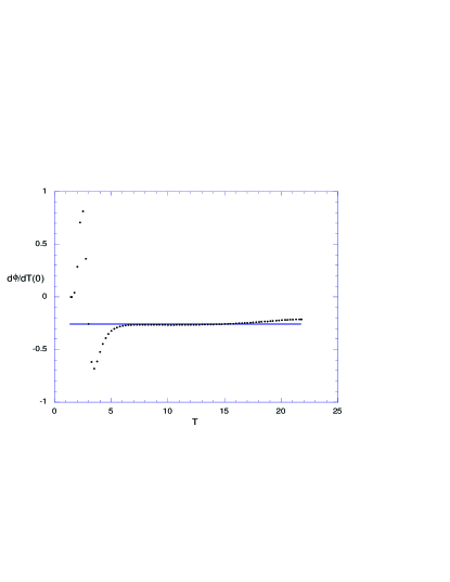
FIG. 1.: numerical values of ${{\left.\partial\phi/\partial T\right|}_{R=0}}$ (dots) with constant (line) approximation to intermediate time behavior

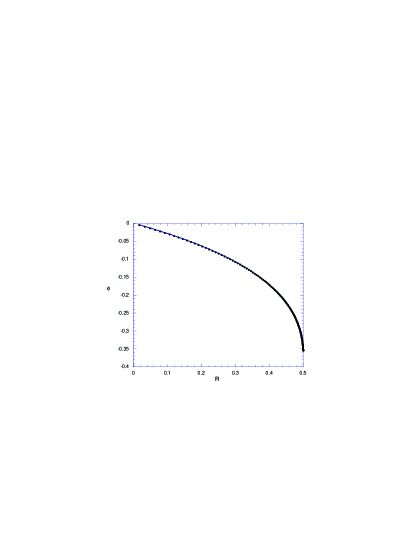
FIG. 2.: comparison of analytic (curve) and numerical (dots) values of the scalar field at an intermediate time

Our solution has an unknown parameter $c$, which should be chosen for best fit with the numerical results. To make this choice, we note that the analytical solution (equation (18)) satisfies $c={{\left.\partial\phi/\partial T\right|}_{R=0}}$. Thus the values of ${\left.\partial\phi/\partial T\right|}_{R=0}$ for the numerical solution should allow us to determine the value of $c$. Figure 1 shows a plot of ${\left.\partial\phi/\partial T\right|}_{R=0}$ vs $T$ for the numerical solution. Note that there is a range of intermediate times for which this quantity is approximately constant. The line in the solution corresponds to the value of $c$ given by equation (25) with $n=4$. While it is not necessary that $c$ be given by equation (25), we find that this particular value of $c$ gives excellent agreement with the numerical data. From now on, we will assume that $c$ has this value.

Figure 2 shows a comparison between the numerical and analytic results for the scalar field $\phi$. Here the dots are the numerical results and the curve is the analytic one. The comparison is made at $T=9$. The freedom to add a constant to the scalar field is used to set the value of the scalar field to zero at the origin. Note that there is excellent agreement between analytic and numerical results. Though this figure shows the comparison at only one time, the agreement persists for a large range of intermediate times.

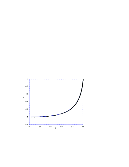
FIG. 3.: comparison of analytic (curve) and numerical (dots) values of the mass aspect at an intermediate time

Due to the symmetry of the spactime, the metric is determined entirely by the matter. This is made explicit in equations (10) and (11). Therefore, since the scalar fields of the numerical and analytic solutions agree, the metrics must agree also. Nonetheless, for illustrative purposes we present a comparison of the metrics of the numerical and analytic solutions. Figure 3 shows a comparison of the quantity $M=({{\bar{r}}^{2}}/{l^{2}})-({\bar{g}}/g)$ with the numerical solution given by the dots and the analytic solution given by the curve. Note the excellent agreement between the two solutions. Here the comparison is made at $T=9$, but the agreement persists for a large range of intermediate times. The metric is determined by $M$ and $\bar{g}$ which is 1 for the analytic solution and very close to 1 for the numerical solution in the intermediate range of times. Thus, in the intermediate range of times, the scalar field and metric of the numerical and analytic solutions agree.

In figures 2 and 3, we have performed the comparison of analytic and numerical solutions only up to the past light cone of the singularity. However, the numerical solution certainly continues beyond this light cone, and since $q=4$, the analytic solution also extends. Do the two solutions still agree in this region? I argued at the end of the previous section that they cannot agree, since the analytic solution contains a closed trapped surface beyond the light cone. Nonetheless, it would be useful to compare the two solutions in this larger region to see the extent and nature of their disagreement.

To make this comparison, a different coordinate from $R$ is needed, since the solution is not smooth in $R$ across the light cone. Here we use as our new coordinate the affine parameter $\lambda$ along an outgoing radial null geodesic. The affine parameter is made scale invariant by choosing the null geodesic to have inner product $u$ with the central observer. The analytic solution can be expressed parametrically in terms of $\lambda$ as follows: (here we specialize to the case $q=4$). Introduce the variable $x\equiv{{(-u)}^{-1/8}}w$. Then $x=1$ at the origin and $x=0$ at the past light cone of the singularity. We have

$$\lambda={1\over{2{\sqrt{2}}}}{\int_{x}^{1}}{{\left(1+{x^{4}}\right)}^{7/2}}dx$$ (27)

$$\phi={\sqrt{7\over{8\pi}}}\ln\left({{1+{x^{4}}}\over 2}\right)$$ (28)

$$M=-{x^{7}}{{\left({2\over{1+{x^{4}}}}\right)}^{7/2}}$$ (29)

From equation (27) it follows that the past light cone is at $\lambda\approx 0.838$. Using equation (26), the affine parameter $\lambda$ can be found numerically from the numerical data. Note, however that the numerical simulations have only a certain range in $\lambda$ since a critical numerical solution must stop before the time $t$ of singularity formation. In our case, the maximum value of $\lambda$ for the numerical data is approximately 1.

Figures 4 and 5 show a comparison between the numerical and analytic solutions for the range $0\leq\lambda\leq 1$. Here the values of $\phi$ are compared in figure 4, while the mass aspect $M$ is compared in figure 5. As in figures 2 and 3, the comparison is made at $T=9$. From the figures it is not clear whether there is a disagreement between the two solutions in the range $\lambda>0.838$ that is beyond the past light cone. To see the disagreement clearly, one would need a larger range of $\lambda$. This could perhaps be provided by a numerical simulation that used double null coordinates.

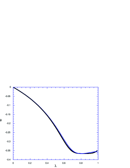
FIG. 4.: comparison of analytic (curve) and numerical (dots) values of the scalar field with respect to affine parameter at an intermediate time

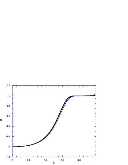
FIG. 5.: comparison of analytic (curve) and numerical (dots) values of the mass aspect with respect to affine parameter at an intermediate time

V Perturbations

We now turn to a treatment of perturbations of the critical solution. This treatment should in principle allow us to determine analytically (1) the correct value of the parameter $c$ and (2) the value of the exponent in scaling relations for near-critical collapse. Unfortunately, as we will see below, it is unclear what boundary conditions to impose on the perturbations.

The critical solution, when perturbed, has one unstable mode that grows as $e^{kT}$ for some constant $k$. Therefore the correct value of $c$ is the one for which there is exactly one unstable mode. The quantity $k$ is related to scaling laws for near-critical collapse. In the collapse of a one parameter family of initial data, a quantity $Q$ with dimension ${({\rm length})}^{s}$ obeys a scaling relation $Q\propto{{|p-{p^{*}}|}^{s/k}}$ where $p$ is the parameter and $p^{*}$ is its critical value. Pretorius and Choptuik[2] examine scaling in maximum scalar curvature for subcritical collapse, a quantity that has dimension ${({\rm length})}^{-2}$. They find $k\approx 0.83$.

In the approximation that ${\bar{g}}=1$, the scalar field satisfies the flat space wave equation. Therefore, the perturbed scalar field $\delta\phi$ also satisfies this equation. Then making the ansatz $\delta\phi={e^{kT}}S(R)$ and using equation (12) we obtain

$$R(1-2R){S^{\prime\prime}}+(1-[3+2k]R){S^{\prime}}-kS=0$$ (30)

The solution is

$$S=F(k,1/2,1,2R)$$ (31)

where $F$ is a hypergeometric function. Writing the hypergeometric function in integral form, we have

$$S={2\over\pi}{\int_{0}^{\pi/2}}{{\left(1-2R{\sin^{2}}\chi\right)}^{-k}}d\chi$$ (32)

In principle, one should now impose boundary conditions on the behavior of the perturbation at $R=1/2$ and these boundary conditions would then determine the allowed values of $k$. Unfortunately, it is not clear what boundary conditions are physically reasonable, since the critical numerical solution should match the analytical solution only for $R<1/2$. Therefore, though we have the solution of the perturbation equation, we cannot use this solution to determine the critical exponent.

VI Acknowledgements

I would like to thank Matt Choptuik and Frans Pretorius for many helpful discussions and for providing the comparison between their numerical work and the exact solution of this paper. This work was partially supported by NSF grant PHY-9722039 to Oakland University.

REFERENCES

- [1] Email: garfinkl@oakland.edu
- [2] M. Choptuik and F. Pretorius, gr-qc/0007008
- [3] M. Choptuik, Phys. Rev. Lett. 70, 9 (1993)
- [4] For a review see C. Gundlach, Adv. Theor. Math. Phys. 2, 1 (1998) and references therein
- [5] A. Abrahams and C. Evans, Phys. Rev. Lett. 70, 2980 (1993)
- [6] R. B. Mann and S. F. Ross, Phys. Rev. D 47, 3319 (1993)
- [7] Y. Peleg and A. Steif, Phys. Rev. D 51, 3992 (1995)
- [8] H. Matschull, Class. Quant. Grav. 16, 1069 (1999)
- [9] D. Birmingham and S. Sen, Phys. Rev. Lett. 84, 1074 (2000)
- [10] D. Christodoulou, Commun. Math. Phys. 105, 337 (1986)
- [11] D. Garfinkle, C. Cutler and G. C. Duncan, Phys. Rev. D 60, 104007 (1999)