Abstract

We investigate the causal structure of the Harada-Iguchi-Nakao (HIN)’s exact solution in detail, which describes the dynamical formation of naked singularity in the collapse of a regular spherical cluster of counterrotating particles. There are three kinds of radial null geodesics in the HIN spacetime. One is the regular null geodesics and the other two are the null geodesics which terminate at the singularity. The central massless singularity is timelike naked singularity and satisfies the strong curvature condition along the null geodesics except for the instant of singularity formation. The cluster dynamically asymptotes to the singular static Einstein cluster in which centrifugal force is balanced with gravity. The HIN solution provides an interesting example which demonstrates that collisionless particles invoke timelike naked singularity.

I Introduction

The cosmic censorship hypothesis (CCH) is one of the most important open problems in general relativity since it plays an important role in theories of black hole physics [1, 2]. The CCH roughly states that singularities forming in gravitational collapse must be hidden behind event horizons and hence invisible to outside observers. Many types of gravitational collapse have been studied so far in the context of the CCH. Some of them produce globally naked singularities, but they cannot immediately be counterexamples to the CCH because the CCH requires suitable matter and appropriate initial conditions.

The well-known example of spacetime which describes the dynamical formation of naked singularity is the Lemaître-Tolman-Bondi (LTB) spacetime [3, 4]. The LTB spacetimes describe the gravitational collapse of a spherically symmetric dust cloud and have an explicit form of the entire spacetime metric. It has been proved that the LTB spacetimes have ingoing null naked singularity from the generic initial data [5, 6, 7, 8, 9, 10]. However this model is rather simplified because pressure is not taken into account.

Some aspects of the effect of pressure on the naked singularity formation have been investigated. Several important results have been obtained. Ori and Piran investigated the spherically symmetric collapse of a perfect fluid numerically under the assumption of self-similarity [11], and analytic discussions based on self-similarity followed it [12]. Harada also solved numerically the non-self-similar spherically symmetric collapse of a perfect fluid [13]. Their results are summarized as that naked singularity can occur in the spherically symmetric collapse of a perfect fluid for a sufficiently soft equation of state. In contrast to isotropic pressure, to include only tangential pressure is turned out to be more tractable [14, 15]. Among the solutions with vanishing radial pressure, there is a system of a spherical cloud of counterrotating particles, in which the physical origin of tangential pressure is clear [16, 17, 18, 19]. The each particle in the cluster has its angular momentum so that the average effect of all particles is a non-vanishing tangential pressure. This model is particularly interesting from a physical point of view because it gives insights into rotational effects on the gravitational collapse, without raising terrible difficulties. Harada, Iguchi and Nakao (HIN) have recently analyzed singularity occurrence in this model [20, 21]. Using the mass-area coordinates, which were first introduced by Ori [22] and were applied in this system by Magli [23], HIN found a new exact solution that describes dynamical formation of massless naked singularity. The results show that the counter-rotation undresses the covered singularity, and in particular tangential pressure and rotation may induce the formation of naked singularity. Since the HIN solution is given in the mass-area coordinates, the motion of each shell and the global properties of the spacetime are not trivial. We study in this paper the HIN solution in detail to make them clear.

The plan of this paper is as follows. In the next section, we review the HIN solution. In Sec. III, we study null geodesics in the HIN spacetime which are necessary to determine the causal structure of spacetime. It is discussed in Sec. IV that the central singularity is timelike. In Sec. V, we will see that the collapse asymptotes to the singular static Einstein cluster. Section VI is devoted to conclusions. We use units with $c=G=1$ and follow the sign conventions of the textbook by Misner, Thorne and Wheeler about the metric, Riemann and Einstein tensors [24].

II The HIN spacetime

A The HIN solution

The HIN solution is the spherical cloud of counterrotating particles which is marginally bound. The specific angular momentum $L(r)$ of each particle at comoving radius $r$ equals to $4F(r)$ [20], where $F(r)$ is the conserved Misner-Sharp mass function [25]. Using comoving coordinates, the line element for this system is reduced to

$$ds^{2}=-e^{2\nu(t,r)}dt^{2}+R^{\prime}{}^{2}(t,r)\left(1+\frac{16F^{2}(r)}{R^{2}(t,r)}\right)dr^{2}+R^{2}(t,r)(d\theta^{2}+\sin^{2}\theta d\phi^{2}),$$ (1)

where $\nu(t,r)$ and $R(t,r)$ satisfy the following set of coupled partial derivative equations:

$$\nu^{\prime}(t,r) = \frac{16F^{2}}{R(R^{2}+16F^{2})}R^{\prime}(t,r),$$ (2)

$$V \equiv e^{-\nu}\dot{R}(t,r)=-\frac{|R-4F|\sqrt{2F}}{\sqrt{R(R^{2}+16F^{2})}}.$$ (3)

The prime and overdot denote the partial derivatives with respect to $r$ and $t$, respectively. The energy density $\epsilon(t,r)\equiv-T^{t}_{t}$ and the tangential pressure $\Pi(t,r)\equiv T^{\theta}_{\theta}=T^{\phi}_{\phi}$ are given by

$$\epsilon(t,r) = \frac{F^{\prime}}{4\pi R^{2}R^{\prime}},$$ (4)

$$\Pi(t,r) = \frac{1}{2}\frac{16F^{2}}{R^{2}+16F^{2}}\epsilon.$$ (5)

Using the coordinate transformation $m=F(r)$ and $R=R(t,r)$, the HIN solution is given in the mass-area coordinates $(m,R)$ by

$$ds^{2}=-Adm^{2}-2BdRdm-CdR^{2}+R^{2}(d\theta^{2}+\sin^{2}\theta d\phi^{2}),$$ (6)

where $A$, $B$ and $C$ are given by

$$A = H\left(1-\frac{2m}{R}\right),$$ (7)

$$B = -\frac{R}{|R-4m|}\sqrt{\frac{RH}{2m}},$$ (8)

$$C = \frac{1}{V^{2}}=\frac{R(R^{2}+16m^{2})}{2m(R-4m)^{2}},$$ (9)

$$\sqrt{H(m,R)} \equiv \sqrt{B^{2}-AC}=\frac{(F^{-1})_{,m}((F^{-1})^{2}+16m^{2})}{|F^{-1}-4m|\sqrt{2mF^{-1}}}$$ (12)

$${}+\mbox{sign}(F^{-1}-4m)\left[\left(\frac{R^{2}-16mR+144m^{2}}{3\sqrt{2}m(R-4m)}\sqrt{\frac{R}{m}}+4\sqrt{2}\ln\frac{\sqrt{R}+2\sqrt{m}}{|\sqrt{R}-2\sqrt{m}|}\right)\right.$$

$$\left.{}-\left(\frac{(F^{-1})^{2}-16mF^{-1}+144m^{2}}{3\sqrt{2}m(F^{-1}-4m)}\sqrt{\frac{F^{-1}}{m}}+4\sqrt{2}\ln\frac{\sqrt{F^{-1}}+2\sqrt{m}}{|\sqrt{F^{-1}}-2\sqrt{m}|}\right)\right].$$

We denote the inverse function of $F(r)$ as $F^{-1}=F^{-1}(m)$ and have set $R=F^{-1}(m)$ on the initial spacelike hypersurface, which corresponds to $R(0,r)=r$. The energy density in the mass-area coordinates is given by

$$\epsilon(R,m)=\frac{\sqrt{R^{2}+16m^{2}}}{4\pi R^{3}|V|\sqrt{H}}.$$ (13)

We can assume that the metric functions are $C^{\infty}$ class with respect to the local Cartesian coordinates at least in the neighborhood of the center $r=0$ before encountering a central singularity. By this assumption, the metric variables in the comoving coordinates are expanded near the center as

$$\nu(t,r) = \nu_{0}(t)+\nu_{2}(t)r^{2}+\nu_{4}(t)r^{4}+O(r^{6}),$$ (14)

$$R(t,r) = R_{1}(t)r+R_{3}(t)r^{3}+R_{5}(t)r^{5}+O(r^{7}).$$ (15)

Then from Eq. (3), the arbitrary mass function $F(r)$ is also expanded as

$$F(r)=F_{3}r^{3}+F_{5}r^{5}+F_{7}r^{7}+O(r^{9}),$$ (16)

and the inverse function $F^{-1}(m)$ is approximately given by

$$F^{-1}(m)=r=\left(\frac{m}{F_{3}}\right)^{1/3}-\frac{F_{5}}{3{F_{3}}^{2}}m+\frac{4{F_{5}}^{2}-3F_{3}F_{7}}{9{F_{3}}^{11/3}}m^{5/3}+O(m^{7/3}),$$ (17)

where we expand $F^{-1}(m)$ up to the order of $m^{5/3}$ because all terms up to this order are needed for later calculations. We can set $\nu_{0}(t)=0$ by using the rescaling freedom of the time coordinate, and Eq. (2) yields $\nu_{2}(t)=0$ . Thus the leading order of $\nu(t,r)$ is given by

$$\nu(t,r)=\frac{4{F_{3}}^{2}}{{R_{1}}^{2}(t)}r^{4}+O(r^{6}).$$ (18)

For $R(t,r)$, we obtain

$$R(t,r)=\left[1-\frac{t}{t_{0}}\right]^{2/3}r+O(r^{3}),$$ (19)

where $t_{0}$ is given by

$$t_{0}=\frac{1}{3}\sqrt{\frac{2}{F_{3}}}.$$ (20)

The break down of these expansions means the appearance of central singularity. Since the break down is given by $R_{1}(t)=0$, the singularity formation time is $t=t_{0}$.

On the initial spacelike hypersurface, the regularity requires $R(t=0,r)=r>4F={O}(r^{3})$ in a sufficiently small, but finite region around $r=0$. From Eq. (3), $R(t,r)$ is a monotonically decreasing function with respect to $t$, and then each initially collapsing shell approaches $R=4F$. Using proper time $\tau(t,r)=\int e^{\nu}dt$ of each shell, the behavior of this approach is

$$R-4F\propto\exp\left(-\frac{\tau}{8F}\right).$$ (21)

This behavior shows that $R$ approaches $4F$ asymptotically and thus $R$ is always $R\geq 4F$ if it initially holds. Since the trapped region is given by $0\leq R<2F$, the region around the center is not trapped eternally. Hence the central singularity is globally naked.

B Algebraic root equation method

The nakedness of the central singularity in the HIN spacetime is also confirmed by examining the algebraic root equation, which probes the existence of outgoing radial null geodesics from the center [8, 9, 10, 23]. To obtain the root equation, consider the radial null geodesic equation in mass-area coordinates

$$\frac{dR}{dm}=\frac{-B\mp\sqrt{H}}{C}=J_{\mp}\sqrt{H(m,R)}\,,$$ (22)

where $J_{\mp}$ is given by

$$J_{\mp}\equiv|V|\left(\frac{R}{\sqrt{R^{2}+16F^{2}}}\mp|V|\right)=\frac{|z-1|}{(z^{2}+1)\sqrt{2z}}\left(z\mp\frac{|z-1|}{\sqrt{2z}}\right),$$ (23)

and we have defined $z\equiv R/4m(\geq 1)$ for later convenience. The upper and lower signs refer to outgoing and ingoing null geodesics in the collapse phase, respectively. Hereafter we use this sign convention. To investigate the behavior of null geodesics near the center, we define

$$x(m)=\frac{R}{2m^{\alpha}},$$ (24)

where $\alpha$ is a constant. Applying l’Hospital theorem to Eq. (24), we obtain the root equation

$$x_{0} = \lim_{m\to 0}\frac{m^{1-\alpha}}{2\alpha}\frac{dR}{dm}$$ (25)

$$= \lim_{m\to 0}\frac{m^{3(1-\alpha)/2}(x_{0}-2m^{1-\alpha})}{2\alpha\,x_{0}\left({x_{0}}^{2}+4m^{2(1-\alpha)}\right)}\,\sqrt{H(m,2x_{0}\,m^{\alpha})}\left[x_{0}^{3/2}\mp m^{(1-\alpha)/2}(x_{0}-2m^{1-\alpha})\right],$$ (26)

where $x_{0}\equiv x(0)$ is introduced. If we find a consistent set of $x_{0}$ and $\alpha$, we have null geodesics which behave as Eq. (24) terminating at the center $m=0$. The root equation method picks up only the geodesics behaving as Eq. (24). To find the another possible null geodesics, we must solve the null geodesic equation.

III Null geodesics in the HIN spacetime

From the detailed analysis of Eq.(26), we can prove that all possible values of $\alpha$ for positive finite $x_{0}$ are 1/3, 7/9 and 1. In reality, these three values of $\alpha$ correspond to three different types of null geodesics in the HIN spacetime, and it will be proved in this section that there are no other null geodesics in the HIN spacetime. We will see below the derivations and properties of these three types of null geodesics in detail.

A $\alpha=1/3$ : regular null geodesics

The null geodesics with $\alpha=1/3$ correspond to regular null geodesics. For this case, the value of $x_{0}$ for $\alpha=1/3$ cannot be determined by the root equation method. We will see that the regular null geodesics actually have $\alpha=1/3$. From Eqs. (1), (18) and (19), the radial null geodesic equation for lowest order is

$$\frac{dt}{dr}\approx\pm\left[1-\frac{t}{t_{0}}\right]^{2/3}.$$ (27)

Inserting the solution $t=t(r)$ of Eq. (27) to Eq. (19), we obtain the regular null geodesics in the mass-area coordinates

$$R(m)\approx\left(1-\frac{t(0)}{t_{0}}\right)^{2/3}\left(\frac{m}{F_{3}}\right)^{1/3},$$ (28)

where $t(0)<t_{0}$ is the time when the null geodesics arrive at or emanate from the regular center $r=0$. The arbitrariness of $x_{0}$ for $\alpha=1/3$ comes from the arbitrary constant $t(0)$ of Eq. (28).

We can find that the scalar curvature is finite at the center along these null geodesics (see Appendix A). In fact, we can prove that all the null geodesics with $\alpha=1/3$ terminate at or emanate from the regular center. The integration of Eq. (3) by using the proper time $\tau(t,r)$ is

$$\tau(t,r)=c(m)-4m\int^{z}_{R_{0}(m)/4m}\frac{\sqrt{2s(s^{2}+1)}}{s-1}ds,$$ (29)

where $R_{0}(m)$ is the initial area radius $R(0,r)=F^{-1}(m)$ and $c(m)$ is an arbitrary function of $m$. For the regular spacetime, $\nu(t,0)=\nu_{0}(t)=0$ implies that we can set $\tau=t$ on $m=0$. Then the singularity appears on $m=0$ when the proper time is $\tau=t_{0}$. The elliptic integral of Eq. (29) is explicitly integrated by approximating the integrand. $R_{0}(m)/4m\gg 1$ is satisfied around the regular center $m=0$ and if we consider the condition $z\gg 1$, the integrand of Eq. (29) is approximately $\sqrt{2s}$. Then, $\tau$ for each shell becomes

$$\tau\approx c(m)+t_{0}-\frac{\sqrt{2}}{3}\left(\frac{R}{m^{1/3}}\right)^{3/2}.$$ (30)

We consider the null geodesics of Eq. (24) for $\alpha={1/3}$. From Eq. (30), the proper time along these geodesics is

$$\tau=c(m)+t_{0}-\frac{4}{3}x^{3/2}.$$ (31)

For the regular shell motion of Eq. (19), Eq. (30) becomes

$$\tau=c(m)+t.$$ (32)

Taking into account $\tau=t$ on $m=0$, we have $c(0)=0$ and thus Eq. (31) implies $\tau<t_{0}$ at $m=0$. Therefore all the null geodesics behaving as $R\propto m^{1/3}$ terminate at $m=0$ before the singularity appears.

B $\alpha=7/9$ : the earliest singular null geodesic

The singular null geodesic with $\alpha=7/9$ for both ingoing and outgoing geodesics was found by Harada, Iguchi and Nakao [20]. The behavior of the null geodesic as

$$R\approx 2x_{0}m^{7/9},$$ (33)

is not regular and thus it terminates at the central singularity. The coefficient $x_{0}$ is given by

$$x_{0}=\left(\frac{24F_{3}^{2}-F_{5}}{4\sqrt{2}F_{3}^{13/6}}\right)^{2/3},$$ (34)

for $F_{5}<24{F_{3}}^{2}$. Note that $F_{5}<24{F_{3}}^{2}$ is the same as the requirement of no shell-crossing singularity and this condition holds if $\epsilon(0,r)$ is a non-increasing function of $r$. It is found that Eq. (30) reduces to $\tau=t_{0}$ at $m=0$ for $\frac{1}{3}<\alpha<1$. Thus all the null geodesics of $\frac{1}{3}<\alpha<1$, particularly $\alpha=7/9$, terminate at the singularity. The scalar curvature diverges along the null geodesic with $\alpha=7/9$ (see Appendix A).

We will see below that there is only one ingoing or outgoing null geodesic with $\alpha=7/9$ and that this null geodesic is the first one which arrives at or emanates from the singularity at $t=t_{0}$. The null geodesic equation in mass-area coordinates has a singular point at $(m,R)=(0,0)$. To make the singular point tractable, we introduce new coordinates as

$$\chi \equiv m^{1/9},$$ (35)

$$\vartheta \equiv \left(\frac{R}{m^{7/9}}\right)^{3/2},$$ (36)

and then Eq. (22) becomes

$$\frac{d\vartheta}{d\chi}+\frac{6}{\chi}(\vartheta-\lambda)=\lambda\Psi_{\mp}(\chi,{\vartheta}),$$ (37)

where $\Psi_{\mp}$ is given by

$$\Psi_{\mp}(\chi,\vartheta) = \frac{1}{\chi}\left(\frac{\psi_{\mp}(\chi,\vartheta)}{\lambda}-6\right),$$ (38)

$$\psi_{\mp}(\chi,{\vartheta}) = \frac{9}{2}\left(3\chi^{2}\vartheta^{1/3}\sqrt{H(\chi,{\vartheta})}J_{\mp}(\chi,{\vartheta})-\vartheta\right),$$ (39)

and we have introduced a parameter $0<\lambda<\infty$.

The form of Eq. (37) is similar to the form of the null geodesic equation of the LTB spacetime given in [6, 7]. One may now follow to Christodoulou’s argument to show the existence and uniqueness of a continuous solution of Eq. (37) [6]. It is sufficient to consider the null geodesic equation in the neighborhood of the center $\chi=0$ since we are interested in the radial null geodesics terminating at $\chi=0$. There is no singular point at $\chi>0$ where $\vartheta$ is strictly positive by definition. Problems appear when we consider the center $\chi=0$. We expand $J_{\mp}$ and $\sqrt{H}$ around $\chi=0$ using Eq. (17),

$$J_{\mp} \approx \sqrt{2}\left(\frac{\chi}{\vartheta^{1/3}}\right)\mp 2\left(\frac{\chi}{\vartheta^{1/3}}\right)^{2}-4\sqrt{2}\left(\frac{\chi}{\vartheta^{1/3}}\right)^{3}+{O}\left(\left(\frac{\chi}{\vartheta^{1/3}}\right)^{4}\right),$$ (40)

$$\sqrt{H} \approx \frac{8{x_{0}}^{3/2}}{9}\frac{1}{\chi^{3}}+\frac{1}{3\sqrt{2}}\left(\frac{\vartheta^{1/3}}{\chi}\right)^{3}-2\sqrt{2}\left(\frac{\vartheta^{1/3}}{\chi}\right)+{O}(\chi^{3})+{O}\left(\frac{\chi}{\vartheta^{1/3}}\right),$$ (41)

and from this expansion, $\psi_{\mp}$ is

$$\psi_{\mp}(\chi,{\vartheta})\approx\psi_{0}+\psi_{1}(\vartheta)\chi+\psi_{2}(\vartheta)\chi^{2}+{O}(\chi^{3}),$$ (42)

where the coefficients of each order are

$$\psi_{0} = 12\sqrt{2}\,x_{0}^{3/2},$$ (43)

$$\psi_{1}(\vartheta) = \mp\frac{\,\vartheta^{2/3}}{\sqrt{2}}\left(9+\frac{2\psi_{0}}{\vartheta}\right),$$ (44)

$$\psi_{2}(\vartheta) = -12\vartheta^{1/3}\left(6+\frac{\psi_{0}}{3\vartheta}\right).$$ (45)

If we choose the parameter $\lambda$ to be $\lambda=\lambda_{0}\equiv(2x_{0})^{3/2}$, $\Psi_{\mp}$ is at least $C^{1}$ in $\chi\geq 0,\vartheta>0$. We can apply the contraction mapping principle to Eq. (37) to find that there exists the solution satisfying $\vartheta(0)=\lambda_{0}$, and moreover that it is the unique solution to Eq. (37) which is continuous at $\chi=0$. This solution with $\vartheta(0)=\lambda_{0}$ exactly agrees with the geodesics of Eq. (33). The proof is presented in Appendix B. Therefore there is no other solution with $0<\vartheta(0)<\infty$. In other words, another possible solution must be $\vartheta(0)=0$ or $\infty$.

We consider possible solutions with $\vartheta(0)=\infty$. When $\vartheta(0)=\infty$, Eq. (37) is approximated around $\chi=0$ by using Eqs. (40) and (41) which are valid even in this limit as follows:

$$\frac{d\vartheta}{d\chi}\approx-\frac{6\vartheta}{\chi}.$$ (46)

The integration of this equation gives $\vartheta(\chi)\propto 1/{\chi}^{6}$. This behavior coincides with the regular null geodesics of Eq. (28) because all the geodesics behaving as $R\propto m^{1/3}$ terminate at the regular center as we have shown before.

It is important that $R(t,r)$ is a monotonically decreasing function with respect to $t$, and thus that $\vartheta$ decreases as $t$ increases when $\chi$ is fixed. Because of this time direction in the mass-area coordinates and the fact that there are no other null geodesics with $(2x_{0})^{3/2}<\vartheta(0)<\infty$, the geodesic with $\vartheta(0)=(2x_{0})^{3/2}$ is the first null geodesic which arrives at or emanates from the appeared singularity. Hence we conclude that the arrival or emanational time in comoving coordinates is the singularity formation time $t=t_{0}$.

C $\alpha=1$ : later singular null geodesics

There are also null geodesics with $\alpha=1$. $x(m)$ is expressed for $\alpha=1$ by a non-analytic function

$$x(m)\approx 2+2\exp\left(-\frac{D}{\sqrt{m}}\right),$$ (47)

where $D$ is the positive constant which parameterizes the null geodesics. We find that the scalar curvature diverges at the center along these null geodesics as is seen in Appendix A. We will see these null geodesics in detail below.

In the coordinate $\vartheta$, these null geodesics are described by solutions with $\vartheta(0)=0$ if they exist. We first search the solution with $z(0)=\infty$ and $\vartheta(0)=0$. Under these conditions, Eq. (22) reduces around $m=0$ to

$$\frac{dz}{dm}=\frac{1}{4m}\left(\sqrt{H}\,J_{\mp}-4z\right)\approx\frac{1}{m\sqrt{z}}\left(\frac{\sqrt{2}{x_{0}}^{3/2}}{9}m^{-1/3}-\frac{2}{3}z^{3/2}\right).$$ (48)

For $z^{3/2}\ll m^{-1/3}$, we can neglect the second term of Eq. (48) and immediately integrate it. However, the solution contradicts $z^{3/2}\ll m^{-1/3}$ because it is given by $z\propto m^{-2/9}$. For $z^{3/2}\propto m^{-1/3}$ or $z^{3/2}\gg m^{-1/3}$, there are consistent solutions. The solution of Eq. (48) for $z^{3/2}\gg m^{-1/3}$ is

$$z\propto\frac{1}{m^{2/3}},$$ (49)

which corresponds regular null geodesics with $\alpha=1/3$. When $z^{3/2}\propto m^{-1/3}$, the integration gives

$$z\propto m^{-2/9},$$ (50)

which corresponds to the unique null geodesic with $\alpha=7/9$. These two solutions satisfy the condition $z(0)=\infty$, but do not satisfy $\vartheta(0)=0$. Consequently there is no solution which satisfies these two conditions.

We consider the geodesics with $z(0)<\infty$ and $\vartheta(0)=0$. Using l’ Hospital theorem, we obtain a restriction on $J_{\mp}\sqrt{H}$ as

$$4z(0)=\lim_{m\to 0}\frac{dR}{dm}=\lim_{m\to 0}J_{\mp}\sqrt{H}<\infty.$$ (51)

Though $J_{\mp}$ is strictly positive at $m=0$ as long as $z(0)>1$, $\sqrt{H}$ diverges to positive infinity at $m=0$ as

$$\sqrt{H}=4\sqrt{2}\left(\frac{\beta}{m^{1/3}}+\gamma m^{1/3}+{O}(m)\right)+\frac{4\sqrt{2}}{3}\frac{\sqrt{z}(z^{2}-4z+9)}{z-1}+4\sqrt{2}\ln\frac{\sqrt{z}+1}{\sqrt{z}-1},$$ (52)

where we have defined

$$\beta \equiv \frac{\sqrt{2}}{9}x_{0}^{3/2},$$ (53)

$$\gamma \equiv -\frac{1440{{{F_{3}}}^{4}}+48\,{{{F_{3}}}^{2}}\,{F_{5}}-17\,{{{F_{5}}}^{2}}+12{F_{3}}{F_{7}}}{216{{F_{3}}}^{23/6}}.$$ (54)

Thus, there exists no solution with the boundary condition $1<z(0)<\infty$. However it may be possible for null geodesics to satisfy Eq. (51) only if $z(0)=1$.

We introduce the new coordinate $y\equiv z-1$ to study the solution $y(m)$ with $y(0)=0$. By expanding Eq. (22) around $y=0$, we obtain the consistent solution with $y(0)=0$ in the lowest order approximation. We give here the null geodesic equation which is expanded up to the enough order so that the difference between ingoing and outgoing null geodesics appears in the expansion;

$$\frac{dy}{dm}\approx\frac{y}{2m}\left(-\ln y+\frac{\beta}{m^{1/3}}+\delta\mp\sqrt{2}+{\gamma}\,m^{1/3}\right).$$ (55)

It can be integrated to

$$y\approx\exp\left(-\frac{D}{\sqrt{m}}+\frac{3\beta}{m^{1/3}}+\delta\mp\sqrt{2}+\frac{3\gamma}{5}\,m^{1/3}\right),$$ (56)

where $D>0$ is an integration constant and $\delta$ is defined as $\delta\equiv 2\ln 2-\frac{8}{3}$. We will see in Sec. V that the constant $D$ is related to the time when the null geodesics terminate at the center $m=0$. The geodesics of Eq. (56) satisfy $y(0)=0$ and they are classified into the geodesics with $\alpha=1$. To obtain the proper time when the null geodesics terminate at the singularity, we consider Eq. (29) again. By the approximation of the integrand, Eq. (29) reduces around $m=0$ to

$$\tau\approx c(m)-4m\left(2\ln y(m)-\frac{t_{0}}{4m}\right).$$ (57)

Then the proper time when the null geodesics terminate at $m=0$ is $\tau=t_{0}$ and it means that the null geodesics terminate at the central singularity. As a result, it is concluded that all the solutions with $\vartheta(0)=0$ are the solutions which terminate at the singularity with $y(0)=0$.

IV Causal structure of the HIN spacetime

A Timelike singularity

It is important that Eq. (56) includes all the null geodesics emanating from the center after the singularity appears. We construct double null coordinates by using Eq. (56) and study the causal structure of the spacetime which is covered by these null geodesics. From Eq. (56), we introduce double null coordinates $(u,v)$ which satisfy around $m=0$

$$2\sqrt{2}u \approx \sqrt{m}\left(-\ln y+\frac{3\beta}{m^{1/3}}+\delta-\sqrt{2}+\frac{3\gamma}{5}\,m^{1/3}\right),$$ (58)

$$2\sqrt{2}v \approx \sqrt{m}\left(-\ln y+\frac{3\beta}{m^{1/3}}+\delta+\sqrt{2}+\frac{3\gamma}{5}\,m^{1/3}\right).$$ (59)

Then, $m$ and $y$ are expressed in the null coordinates by

$$\sqrt{m} \approx v-u,$$ (60)

$$y \approx \exp\left(-\frac{\sqrt{2}(v+u)}{v-u}+\frac{3\beta}{(v-u)^{2/3}}+\delta+\frac{3\gamma}{5}\,(v-u)^{2/3}\right).$$ (61)

We are considering a sufficiently small, but finite region around $m=0$. Then Eq. (60) restricts $u$ and $v$ to $u\approx v$. From Eqs. (60) and (61), $dm$ and $dR$ are given by

$$dm \approx 2(v-u)(dv-du),$$ (62)

$$dR-4dm \approx -4\sqrt{2}y\left(v+u-\sqrt{2}\beta(v-u)^{1/12}+(\sqrt{2}+1)(v-u)+\frac{\sqrt{2}}{5}\gamma\,(v-u)^{5/12}\right)du$$ (64)

$$+4\sqrt{2}y\left(v+u-\sqrt{2}\beta(v-u)^{1/12}+(\sqrt{2}-1)(v-u)+\frac{\sqrt{2}}{5}\gamma\,(v-u)^{5/12}\right)dv.$$

Inserting Eqs. (62) and (64) into Eq. (6) and expanding the metric functions $A,B$ and $C$ around $(m,y)=(0,0)$, we obtain the line element in the double null coordinates as

$$ds^{2}\approx-512(v-u)^{2}dvdu+R^{2}(d\theta^{2}+\sin^{2}\theta d\phi^{2}).$$ (65)

The details of the calculation are given in Appendix C. In the null coordinates, the central singularity is represented at $u=v$ which corresponds to the center $m=0$ because of Eq. (60). It is found that the world line of $u=v$ is timelike. Hence the central singularity in the spacetime which is covered by the null geodesics given by Eq. (56) is timelike.

B Penrose diagram

Here we summarize the obtained results. The whole of the spacetime is covered by three types of null geodesics which can be classified by the value of $\alpha$ into $\alpha=1/3$, $7/9$ and $1$. The null geodesics with $\alpha=1/3$ emanate from or terminate at the regular center and they are parametrized by one parameter. There is only one null geodesic with $\alpha=7/9$ and it is the earliest one which emanates from or terminates at the naked singularity. The null geodesics with $\alpha=1$ emanate from or terminate at the timelike singularity and they are parametrized by one parameter. From these results, it is now possible to draw the conformal diagram of the HIN spacetime (see Fig. 1). For comparison, we also present the conformal diagram of the LTB spacetime with naked singularity (see Fig. 2). It is found that the effect of counterrotation makes the singularity timelike in this model.

C Curvature strength of the singularity

We should note the curvature strength of the singularity in the HIN spacetime. According to Tipler and Królak, we classify the curvature strength whether the singularity satisfies the strong curvature condition (SCC) or the limiting focusing condition (LFC) [26, 27]. Harada, Nakao and Iguchi studied the SCC and the LFC for spherically symmetric spacetimes with vanishing radial pressure [28]. Applying theorems 1, 2 and 3 of their paper to the HIN spacetime, we can know the curvature strength along each null geodesic. For $\alpha=7/9$, not the SCC but only the LFC is satisfied along the null geodesics. For $\alpha=1$, the SCC is satisfied along the null geodesics. In conclusion, the naked singularity is relatively weak at the formation but becomes strong after that.

V Asymptotic Behavior

It is worth while examining the asymptotic behavior of the spacetime. We concern with the null geodesic behavior in the comoving coordinates corresponding to Eq. (56). To obtain an insight, we consider the asymptotic behavior of the HIN solution in comoving coordinates. Since the time coordinate $t$ at the center does not proceed after the singularity formation, we must introduce new time coordinate which no longer agrees with the proper time at $r=0$. We denote the new time coordinate as $T$ and consider that the time $t$ in Eqs. (1), (2) and (3) is replaced by $T$.

We take the limit $R=4F$ because $R(T,r)$ approaches $4F(r)$ asymptotically. From Eq. (2), the metric in this limit is given by

$$ds^{2}=-\frac{4F(r)}{K(T)}dT^{2}+2(4F^{\prime}(r))^{2}dr^{2}+(4F(r))^{2}(d\theta^{2}+\sin^{2}\theta d\phi^{2}).$$ (66)

The function $K(T)$ is an arbitrary function of $T$ which comes from the integration of Eq. (2). For simplicity we set $K(T)=K=constant$ by rescaling the time coordinate. The energy density in this limit is

$$\epsilon = \frac{1}{256\pi F^{2}}.$$ (67)

This solution is a static system of counterrotating particles, which is called the Einstein cluster. In particular, the solution has timelike naked singularity at the center.

To study the asymptotic behavior of the shell motion for fixed $r$, we set perturbed quantities $e(T,r)$ and $d(T,r)$ for the coordinates $(T,r)$ around $R=4F$ as,

$$R(T,r) = 4F(r)\left[1+e(T,r)\right],$$ (68)

$$e^{2\nu(T,r)} = e^{d(T,r)}\frac{R(T,r)}{K}\approx\frac{4F(r)}{K}[1+e(T,r)+d(T,r)].$$ (69)

Inserting these quantities into Eqs. (2) and (3), we obtain following perturbed equations in linear order,

$$\dot{e}(T,r) = -\frac{e(T,r)}{4\sqrt{KF(r)}},$$ (70)

$$d^{\prime}(T,r) = -\frac{F^{\prime}(r)}{F(r)}e(T,r).$$ (71)

The solutions of these equations are

$$e(T,r) = E(r)\exp\left(-\frac{T}{4\sqrt{KF(r)}}\right),$$ (72)

$$d(T,r) = -\int e(T,r)\frac{F^{\prime}}{F}dr+G(T),$$ (73)

where $E(r)$ and $G(T)$ are arbitrary functions of the comoving radius $r$ and time $T$ respectively. We have implicitly assumed that the time $T$ is very large compared to the singularity formation time. However, Eqs. (72) and (73) imply that this perturbation scheme is valid soon after the singularity formation time as long as we consider the region in which the radius $r$ is very small.

In the asymptotic region, the proper time becomes

$$\tau(T,r)=2\sqrt{\frac{F}{K}}\,\left[\,T+const.+{O}\left(e(T,r)\right)\,\right].$$ (74)

It is found that the asymptotic behavior of Eqs. (72) and (74) completely coincides with the already obtained behavior of Eq. (21). Using these results of perturbation, the null geodesic equation in the comoving coordinates is

$$\frac{dT}{dr}=\pm\sqrt{\frac{2K}{F}}\Bigl{(}2F^{\prime}+2Fe^{\prime}-F^{\prime}d\Bigr{)},$$ (75)

and it is immediately integrated to

$$T(r)=T(0)\pm\sqrt{2K}\left(4\sqrt{F(r)}+\int\frac{dr}{\sqrt{F(r)}}\left[2Fe^{\prime}-F^{\prime}d\,\right]\right).$$ (76)

Integration constant $T(0)$ is the time when these null geodesics terminate at or emanate from the singularity, and this parameterization of the null geodesic family corresponds to the fact that the singularity is timelike. From Eqs. (68), (72) and (76), we obtain the null geodesics in the mass-area coordinates corresponding to Eq. (76),

$$y=\frac{R}{4F}-1=E(r)\exp\left(-\frac{T(0)}{4\sqrt{KF(r)}}\mp\sqrt{2}\mp\frac{1}{2\sqrt{2F(r)}}\int\frac{dr}{\sqrt{F(r)}}[2Fe^{\prime}-F^{\prime}d\,]\right).$$ (77)

Comparing this result to Eq. (56), the parameter $D$ relates to the arrival time $T(0)$ as $T(0)=4D\sqrt{K}$.

VI Conclusions

We have studied the causal structure of the HIN spacetime and it was shown that the central massless singularity of this spacetime is timelike. To show this fact, we have investigated the radial null geodesics in detail. The null geodesics are classified to three types, $\alpha=$ 1/3, 7/9 and 1, by their dependence of $R$ on $m$ near the center. One is regular and the other two are singular. The classification of the singular geodesics corresponds to their arrival or emanational time at the central singularity. The $\alpha=7/9$ type is the earliest singular null geodesic which arrives at or emanates from the singularity at its formation time $t_{0}$, while the geodesics with $\alpha=1$ arrive at or emanate from the singularity after its appearance.

We have shown that singular null geodesics with $\alpha=1$ exactly parametrized by their arrival or emanational time and that there is only one set of ingoing and outgoing geodesics for each parameter. This fact shows that the central singularity has timelike property. We have also constructed double null coordinates around the central singularity from the null geodesics with $\alpha=1$. The line element in this double null coordinates shows that there is timelike singularity in this spacetime. We have considered the asymptotic behavior of this spacetime after the singularity appeared in comoving coordinates. It gives us understanding of the null geodesic behavior in mass-area coordinates, and of the parametrization of the null geodesic family. The curvature strength of this singularity was also investigated. The LFC is satisfied along the null geodesics with $\alpha=7/9$ and the SCC is satisfied for $\alpha=1$. The curvature strength of the naked singularity is relatively weak at the formation and it becomes strong after that.

In summary, the HIN solution describes a dynamical formation of timelike naked singularity, that is, the birth of timelike singularity. The solution dynamically tends to the static singular Einstein cluster as time proceeds. Though the HIN system is simply composed of collisionless particles, the collapse leads to the nontrivial causal structure. It implies that the effects of rotation and tangential pressure play important roles in the final stage of collapse, particularly the singularity formation.

A Scalar Curvature along the null geodesics

Singularities are boundary points of spacetime where the normal differentiability breaks down. If the energy density or the curvature invariant diverges at boundary points, the points are singularities. In this appendix, we give the scalar curvature $R^{\mu}_{\mu}$ in the HIN spacetime along the radial null geodesics terminating at the center $r=0$, and show that the center is singular along the geodesics with $\alpha=7/9$ and $1$.

The scalar curvature $R^{\mu}_{\mu}$ of the HIN spacetime is given by

$$R^{\mu}_{\mu}=\frac{8\pi R^{2}}{R^{2}+16F^{2}}\,\epsilon=\frac{\sqrt{2}}{(R-4m)\sqrt{mR}\sqrt{H}}.$$ (A1)

Along the geodesics $R=2xm^{1/3}$, which are shown to be regular null geodesics, $R^{\mu}_{\mu}$ is given by

$$R^{\mu}_{\mu}=\frac{3}{4x^{3}}+{O}(m^{2/3}),$$ (A2)

and it is finite at $m=0$. On the other hand, when we consider $R^{\mu}_{\mu}$ along the geodesics, $R=2x_{0}m^{7/9}$ and $R=4m(1+y)$ of Eq. (56), the scalar curvatures are given by

$$R^{\mu}_{\mu}=\frac{9}{28{x_{0}}^{3}m^{4/3}}+{O}(m^{-10/9}),$$ (A3)

and

$$R^{\mu}_{\mu}=\frac{1}{64m^{2}}+{O}(m^{-5/2}y),$$ (A4)

respectively. The scalar curvature diverges as $m\to 0$ in these cases, and therefore the center is definitely singular.

B contraction mapping principle

We prove the existence of the unique continuous solution of Eq. (37). It is based on the discussion given by Christodoulou for the LTB model [6]. Consider the differential equation obtained from Eq. (37) by replacing $\vartheta$ in $\Psi_{\mp}(\chi,\vartheta)$ by a given continuous function $\bar{\vartheta}>0$:

$$\frac{d\vartheta}{d\chi}+\frac{6}{\chi}(\vartheta-\lambda_{0})=\lambda_{0}\Psi_{\mp}\left(\chi,\bar{{\vartheta}}(\chi)\right).$$ (B1)

Since we have chosen $\lambda=\lambda_{0}$, $\Psi_{\mp}(\chi,\bar{\vartheta})$ is at least $C^{1}$ in the strip $\chi\in[0,\chi_{1}]$ and $\bar{\vartheta}\in(0,\mu_{1}]$, where we assume $\chi_{1}$ is sufficiently small. The continuous solution of Eq. (B1) is only the solution with $\vartheta(0)=\lambda_{0}(>0)$. This solution is given by

$$\vartheta(\chi)=\lambda_{0}\left(1+\chi\int^{1}_{0}s^{6}\Psi_{\mp}\left(s\chi,\bar{\vartheta}(s\chi)\right)ds\right).$$ (B2)

We consider the nonlinear map $T_{\lambda_{0}}$ defined as $\vartheta=T_{\lambda_{0}}(\bar{\vartheta})$. Since we are considering the function $\bar{\vartheta}$ with $\bar{\vartheta}(0)>0$, we obtain $T_{\lambda_{0}}(\bar{\vartheta})(0)=\lambda_{0}$ from expansions of Eqs. (40) and (41). Thus the possible fixed point of $T_{\lambda_{0}}$ is only one which satisfies ${\vartheta_{\rm{FP}}}(0)=\lambda_{0}$. To prove the existence of the fixed point, we consider the set $V_{\mu}$ consisting of all $\bar{\vartheta}$ such that for $\chi\in[0,\chi_{2}]$,

$$\mu_{-}\leq\bar{\vartheta}(\chi)\leq\mu_{+},$$ (B3)

where the lower and the upper bound are defined by $\mu_{-}\equiv\lambda_{0}-\mu_{2}$ and $\mu_{+}\equiv\lambda_{0}+\mu_{2}$ for a sufficiently small $\mu_{2}$. From these bounds, the nonlinear map is also restricted in

$$\mu_{-}\leq T_{\lambda_{0}}(\bar{\vartheta})(\chi)\leq\mu_{+},$$ (B4)

if we choose a $\chi$ such that

$$\chi\leq\chi_{3}\equiv\frac{7\mu_{2}}{\lambda_{0}\Delta_{1}},$$ (B5)

where

$$\Delta_{1}=\sup_{0\leq\chi\leq\chi_{2}\,}\sup_{\mu_{-}\leq\bar{\vartheta}\leq\mu_{+}}|\Psi_{\mp}|.$$ (B6)

The map $T_{\lambda_{0}}$ sends $V_{\mu}$ into itself for all $\chi_{4}\leq\min\{\chi_{2},\chi_{3}\}$. Let

$$\Delta_{2}=\sup_{0\leq\chi\leq\chi_{2}\,}\sup_{\mu_{-}\leq\bar{\vartheta}\leq\mu_{+}}\biggl{|}\frac{\partial\Psi_{\mp}}{\partial\bar{\vartheta}}\biggr{|}.$$ (B7)

Then we obtain from Eq. (B2) for $\bar{\vartheta}_{1},\,\bar{\vartheta}_{2}\in V_{\mu}$,

$$\|T_{\lambda_{0}}(\bar{\vartheta}_{1})-T_{\lambda_{0}}(\bar{\vartheta}_{2})\|\leq\frac{\chi_{4}\lambda_{0}\Delta_{2}}{7}\|\bar{\vartheta}_{1}-\bar{\vartheta}_{2}\|,$$ (B8)

where $\|$ $\|$ denotes the supremum norm. If we choose $\chi_{4}<7/(\lambda_{0}\Delta_{2})$, the map $T_{\lambda_{0}}$ is contractive in $V_{\mu}$. Hence $T_{\lambda_{0}}$ has a unique fixed point $\vartheta_{\rm{FP}}\in V_{\mu}$ which is given by

$$\vartheta_{\rm{FP}}(\chi)=T_{\lambda_{0}}(\vartheta_{\rm{FP}})(\chi)=\lambda_{0}\left(1+\chi\int^{1}_{0}s^{6}\Psi_{\mp}\left(s\chi,\vartheta_{\rm{FP}}(s\chi)\right)ds\right).$$ (B9)

Therefore we have the unique continuous solution with $\vartheta(0)=\lambda_{0}$.

C derivation of eq. (65)

In this appendix, we construct double null coordinates by using Eq. (56). We define double null coordinates $(u,v)$ as Eqs. (58) and (59). From this definition, $dm$ and $dR$ are given by

$$dm = p_{u}du+p_{v}dv,$$ (C1)

$$dR = 4dm+(q_{u}du+q_{v}dv),$$ (C2)

where

$$p_{u} \approx -p_{v}\approx 2(u-v),$$ (C3)

$$q_{u} \approx -4\sqrt{2}y\left(v+u-\sqrt{2}\beta(v-u)^{1/12}+(\sqrt{2}+1)(v-u)+\frac{\sqrt{2}}{5}\gamma\,(v-u)^{5/12}\right)du,$$ (C4)

$$q_{v} \approx 4\sqrt{2}y\left(v+u-\sqrt{2}\beta(v-u)^{1/12}+(\sqrt{2}-1)(v-u)+\frac{\sqrt{2}}{5}\gamma\,(v-u)^{5/12}\right)dv.$$ (C5)

The line element of Eq. (1) is rewritten by the coordinate transformation from $(m,R)$ to $(u,v)$

$$ds^{2} = Udu^{2}+Vdv^{2}+Wdudv+R^{2}d\Omega^{2},$$ (C6)

where the metric functions $U,V$ and $W$ are given by

$$U = -(A+8B+16C)p_{u}^{2}-Cq_{u}^{2}-2(B+4C)p_{u}q_{u},$$ (C7)

$$V = -(A+8B+16C)p_{v}^{2}-Cq_{v}^{2}-2(B+4C)p_{v}q_{v},$$ (C8)

$$W = -2(A+8B+16C)p_{u}p_{v}-2Cq_{u}q_{v}-2(B+4C)(p_{u}q_{v}+p_{v}q_{u}).$$ (C9)

From Eq. (C3), we obtain

$$W\approx-U-V-C(q_{u}+q_{v})^{2},$$ (C10)

and then Eq. (C6) becomes

$$ds^{2}\approx-C(q_{u}+q_{v})^{2}dudv+U(du^{2}-dudv)+V(dv^{2}-dudv)+R^{2}d\Omega^{2}.$$ (C11)

If the condition

$$-C(q_{u}+q_{v})^{2}\gg U,V$$ (C12)

is satisfied, the double null coordinates would be constructed approximately.

We expand $\sqrt{H}$ of Eq. (52) around $y=0$,

$$\sqrt{H}=h(m)+\sqrt{2}\left(\frac{8}{y}-4\,{\ln y}+4\,(3+\delta)+y+\frac{3}{4}y^{2}+O(y^{3})\right),$$ (C13)

where $h(m)$ is defined as

$$h(m)=4\sqrt{2}\left(\frac{\beta}{m^{1/3}}+\,\gamma\,m^{1/3}+{O}(m)\right).$$ (C14)

Inserting Eq. (C13) into $A$, $B$ and $C$, metric functions $U$, $V$ and $W$ are calculated. As a result we obtain

$$\lim_{m\to 0}-\frac{1}{m}C(q_{u}+q_{v})^{2} = -512,$$ (C15)

$$\lim_{m\to 0}\frac{U}{m} = 0,$$ (C16)

$$\lim_{m\to 0}\frac{V}{m} = 0,$$ (C17)

and it satisfies the condition of Eq. (C12). Hence the line element around the center is given by

$$ds^{2}\approx-512(v-u)^{2}\,dudv+R^{2}d\Omega^{2}.$$ (C18)

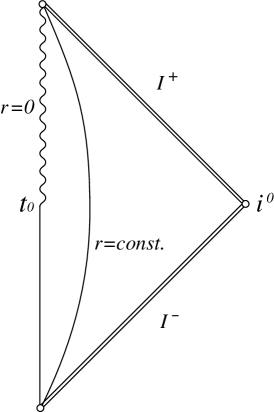
FIG. 1.: The conformal diagram of the HIN spacetime. A timelike naked singularity emerges at the center at $t=t_{0}$. There are one parameter family of both ingoing and outgoing null geodesics which terminate at and emanate from the naked singularity.

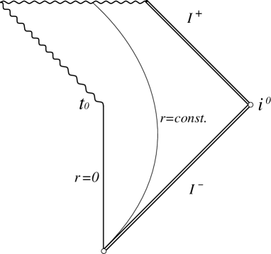
FIG. 2.: The conformal diagram of the LTB spacetime with naked singularity. There are one parameter family of outgoing null geodesics which emanate from the naked singularity but only one ingoing null geodesic which terminates at the naked singularity.

REFERENCES

- [1] R. Penrose, “Singularities and Time Asymmetry”, in General Relativity, an Einstein Centenary Survey, ed. S.W. Hawking and W. Israel, (Cambridge University Press, Cambridge, England), p581, (1979).
- [2] S.W. Hawking and G.F.R. Ellis, The large scale structure of space-time, (Cambridge University Press, Cambridge, England) (1973).
- [3] R. C. Tolman, Proc. Nat. Acad. Sci 20, 169 (1934).
- [4] H. Bondi, Mon. Not. R. Astron. Soc. 107, 410 (1947).
- [5] D.M. Eardly and L. Smarr, Phys. Rev. D 19, 2239 (1979).
- [6] D. Christodoulou, Commun. Math. Phys. 93, 171 (1984).
- [7] R. P. A. C. Newman, Class. Quantum Grav. 3, 527 (1986).
- [8] P.S. Joshi and I.H. Dwivedi, Phys. Rev. D 47, 5357 (1993).
- [9] T.P. Singh and P.S. Joshi, Class. Quantum Grav. 13, 559 (1996).
- [10] S. Jhingan, P.S. Joshi and T.P. Singh, Class. Quantum Grav. 13, 3057, (1996).
- [11] A. Ori and T. Piran, Phys. Rev. Lett. 59, 2137 (1987); Gen. Relativ. Gravit. 20, 7 (1988); Phys. Rev. D 42, 1068 (1990).
- [12] P.S. Joshi and I.H. Dwivedi, Commun. Math. Phys. 146, 333 (1992); Lett. Math. Phys. 27, 235 (1993).
- [13] T. Harada, Phys. Rev. D 58, 104015, (1998).
- [14] T.P. Singh and L. Witten, Class. Quantum Grav. 14, 3489 (1997).
- [15] G. Magli, Class. Quantum Grav. 14, 1937 (1997).
- [16] A. Einstein, Ann. Math. 40, 4, 922 (1939).
- [17] B.K. Datta, Gen. Relat. Grav. 1, 19 (1970).
- [18] H. Bondi, Gen. Relat. Grav. 2, 321 (1971).
- [19] A.B. Evans, Gen. Relat. Grav. 8, 155 (1976).
- [20] T. Harada, H. Iguchi and K. Nakao, Phys. Rev. D 58, 041502, (1998).
- [21] S. Jhingan and G. Magli Phys. Rev. D 61, 124006, (2000).
- [22] A. Ori, Class. Quantum Grav. 7, 985, (1990).
- [23] G. Magli, Class. Quantum Grav. 15, 3215, (1998).
- [24] C. W. Misner, K. S. Thorne and J. A. Wheeler, Gravitation, (W. H. Freeman, San Francisco), (1973).
- [25] C. W. Misner and D. H. Sharp, Phys. Rev. B 136, 571 (1964).
- [26] F. J. Tipler, Phys. Lett. A 64, 8, (1977).
- [27] A. Królak, J. Math. Phys. 28, 138, (1987).
- [28] T. Harada, K. Nakao and H. Iguchi, Class. Quantum Grav. 16, 2785, (1999).