Gravitational and dilaton radiation from a relativistic membrane

Abstract

Recent scenarios of the TeV-scale brane cosmology suggest a possibility of existence in the early universe of two-dimensional topological defects: relativistic membranes. Like cosmic strings, oscillating membranes could emit gravitational radiation contributing to a stochastic background of gravitational waves. We calculate dilaton and gravitational radiation from a closed toroidal membrane excited along one homology cycle. The spectral-angular distributions of dilaton and gravitational radiation are obtained in a closed form in terms of Bessel’s functions. The angular distributions are affected by oscillating factors due to an interference of radiation from different segments of the membrane. The dilaton radiation power is dominated by a few lower harmonics of the basic frequency, while the spectrum of the gravitational radiation contains also a substantial contribution from higher harmonics. The radiative lifetime of the membrane is determined by its tension and depends weakly on the ratio of two radii of the torus. Qualitatively it is equal to the ratio of the membrane area at the maximal extension to the gravitational radius of the membrane as a whole.

I Introduction

Now it is well understood that topological defects which could have been created at the early stages of cosmological expansion may leave their footprints in the spectrum of the background gravitational waves ViSh92 ; BaCaSh97 which can be detected in the future experiments. Until recently main attention was paid to the effects due to cosmic strings. Cosmic strings, presumably serving as seeds for the formation of galaxies, were thought to be produced at the phase transition of the grand unification scale Ki76 ; HiKi95 . Gravitational, dilaton and axion radiation emitted by oscillating strings was thoroughly studied in a number of papers (see e.g. Vi85 ; Bu85 ; VaVi85 ; GaVa87 ; DaVi97 and references therein). Although a recent analysis of the available astrophysical data seems to rule out the cosmic string scenario of the formation of structures in the Universe, these calculations may still be of interest in the context of the fundamental string/M theory.

Recently it was argued that the mass scale of the superstring/M theory may be as low as 10 TeV ArDiDv98 ; AnArDiDv98 at the expense of existence of some non-small extra dimensions. If true, this may drastically modify the full scenario of cosmological evolution. Based on this assumption various cosmological models were envisaged in which the observed Universe is treated as a three-brane embedded in a higher-dimensional world. According to this brane cosmology the standard model particles are confined to the brane while gravity lives in the full space. Such scenarios appeal to reconsider the problem of topological defects which should be associated rather with solitons of the fundamental string theory than with those of the field-theoretical models of grand unification.

Among the string theory solitons which may live on a three-brane there are one-dimensional strings and two-dimensional membranes. In the zero-thickness limit the dynamics of solitonic strings is governed by the Nambu-Goto action, while the membranes are described by a similar three-dimensional geometrical action (see e.g. CoTu76 ; Su83 ). Relativistic membrane in the four-dimensional spacetime geometrically are similar to domain walls encountered in the usual field-theoretical models. However their formation and dynamics in the string/brane cosmology are likely to be different from dynamics of the domain walls in the standard cosmological scenario. Here we do not discuss details of creation and evolution of membranes in the brane cosmology but concentrate on the problem of radiation.

Radiation produced by one-dimensional defects – the relativistic strings – is likely to be similar to radiation from the cosmic strings, apart from a different attribution of scalar and two-form fields involved. Radiation from an oscillating two-dimensional relativistic membrane seems not to have been studied in detail before, although some earlier estimates of gravitational radiation emitted by the cosmic domain walls are worth to be mentioned GlRo98 ; KoTuWa92 . Massless boson modes to which the membranes are coupled in the four-dimensional space-time include a dilaton, a graviton and a Ramond–Ramond three-form. The latter is non-dynamical in four dimensions, so oscillating membranes may emit dilatons and gravitons.

In the classical limit one can describe radiation from a vibrating membrane in a standard way using the retarded solutions of the corresponding wave equations. Unfortunately, contrary to the case of strings, a general solution of the (highly non-linear) membrane equation of motion can hardly be obtained in a closed form. To simplify the problem one can restrict oneself by some particular excitation mode. Here we study the dilaton and gravitational radiation emitted by a toroidal oscillating membrane excited along a homology cycle with the radius much smaller than the second radius of the torus. Under such an assumption the membrane equation of motion can be easily solved, and a closed analytic expression for the spectral power of radiation can be obtained. We analyse in detail the spectral-angular distributions with an emphasis on the effects due to two-dimensional nature of a membrane. Hopefully this simple model correctly describes basic features of the membrane radiation in more general case, although radiation due to more complicated excitation modes is certainly worth to be considered in the future.

The plan of the paper is as follows. In Sec. II we derive the linearized equations for the scalar and gravitational radiation from a membrane source. In Sec. III the solution of the equations of motion for a free toroidal membrane is obtained under an assumption of the relative smallness of the radius of an excited homology cycle. Sec. IV is devoted to an analysis of the dilaton radiation; we derive the spectral-angular distribution in terms of the Bessel’s functions and investigate the role of higher harmonics of the basic oscillation frequency. A simplified expression valid in the high-frequency range of the spectrum is obtained in terms of the MacDonald’s functions. In Sec. V the gravitational radiation is studied along similar lines. The results are summarized and discussed in Sec. VI. Some useful integrals involving Bessel’s functions used in the calculation are given in the Appendix.

II Basic equations

Consider a relativistic membrane $x^{\mu}=z^{\mu}(\sigma^{a}),\;\mu=0,1,2,3,$ propagating in the four-dimensional space-time with the metric $g_{\mu\nu}$ and interacting with the dilaton field $\phi$ (our signature convention is $(+---)$). The corresponding action can be written as a sum

$$S=S_{m}+S_{f}$$ (1)

of the purely geometrical membrane action CoTu76 ; Su83

$$S_{m}=\mu\int\limits{\rm e}^{-\alpha\phi}\sqrt{\gamma}\,d^{3}\sigma,$$ (2)

and the field term

$$S_{f}=\frac{1}{16\pi G}\int\limits\left\{-R+2\partial_{\mu}\phi\partial_{\nu}\phi g^{\mu\nu}\right\}\sqrt{-g}d^{4}x.$$ (3)

Here $\mu$ is the membrane tension parameter of a dimension of the energy per unit area, $\alpha$ is the dilaton coupling constant. In our normalization the dilaton field $\phi$ and the coupling constant $\alpha$ both are dimensionless. The membrane world-volume is parameterized by the internal coordinates $\sigma^{a}=(\tau,\sigma,\rho),\quad a=0,1,2$. The induced metric on the world-volume reads

$$\gamma_{ab}=g_{\mu\nu}\frac{\partial z^{\mu}}{\partial{\sigma^{a}}}\frac{\partial z^{\nu}}{\partial{\sigma^{b}}},$$ (4)

where $\gamma=\det\gamma_{ab}$.

Variation of the action (2) over the space-time coordinates $z^{\mu}$ gives the equation of motion

$$\frac{1}{\sqrt{\gamma}}\partial_{a}\left\{{\rm e}^{-\alpha\phi}\sqrt{\gamma}\gamma^{ab}\partial_{b}\left(z^{\nu}g_{\mu\nu}\right)\right\}=0,$$ (5)

where $\gamma^{ab}$ is the inverse metric on the world-volume. Up to the dilaton factor, this is a three-dimensional covariant D’Alembert equation. It is worth comparing it with the two-dimensional string equation of motion. In the latter case one has three gauge degrees of freedom corresponding to two diffeomorphisms and a Weyl transformation on the world-sheet. Consequently, three independent components of the world-sheet metric can be chosen flat, so that the equation of motion becomes linear. A general solution can be written as a sum of two arbitrary functions of null coordinates on the world-sheet: right and left movers. This is no more possible in the case of a membrane for which the number of gauge degrees of freedom is again three (diffeomorphisms of the world-volume), while the number of the independent world-volume metric components is six. Therefore the membrane equation of motion remains essentially non-linear in any gauge. To make it explicitly solvable one needs additional assumptions to be made about excitation modes.

Variation of the full action (1) with respect to the dilaton $\phi$ gives the four-dimensional D’Alembert equation

$$\frac{1}{\sqrt{-g}}\partial_{\mu}\left(\sqrt{-g}g^{\mu\nu}\partial_{\nu}\phi\right)=4\pi j(x)$$ (6)

with the source term

$$j(x)=G\mu\alpha{\rm e}^{-\alpha\phi}\int\limits\frac{\delta^{4}\left(x-z(\sigma)\right)}{\sqrt{-g}}\sqrt{\gamma}\,d^{3}\sigma.$$ (7)

Note that the effective coupling of the dilaton to the membrane is proportional to the dilaton exponential. In absence of the dilaton background this factor is of course negligible in the linearized limit relevant to the radiation problem.

Finally, varying the action (1) with respect to the space-time metric $g_{\mu\nu}$, one obtains the Einstein equations

$$R_{\mu\nu}-\frac{1}{2}g_{\mu\nu}R=8\pi G\left(T_{\mu\nu}+T^{dil}_{\mu\nu}\right),$$ (8)

with the source term consisting of the membrane stress–tensor

$$T^{\mu\nu}=\mu\int\limits{\rm e}^{-\alpha\phi}\gamma^{ab}\partial_{a}z^{\mu}\partial_{b}z^{\nu}\frac{\delta^{4}\left(x-z(\sigma)\right)}{\sqrt{-g}}\sqrt{\gamma}\,d^{3}\sigma,$$ (9)

and the dilaton term. In what follows we neglect the interaction of the dilaton with gravity and omit the second term. The effective coupling of the membrane to gravity contains again the dilaton exponential factor which may be neglected in absence of the dilaton background.

The action (1) is invariant under the reparameterization of the world-volume $\sigma^{a}\to\sigma^{a^{\prime}}(\sigma^{b})$, so three gauge conditions may be imposed on the world-volume metric $\gamma_{ab}$. We will treat the gravitational field perturbatively on the flat background

$$g_{\mu\nu}=\eta_{\mu\nu}+h_{\mu\nu},$$ (10)

where $\eta_{\mu\nu}$ is the Minkowski metric, and choose the parameterization of the world-volume ensuring diagonality of the metric $\gamma_{ab}$:

$$\dot{z}^{\mu}z^{\prime}_{\mu}=0,\quad{\dot{z}}^{\mu}\bar{z}_{\mu}=0,\quad z^{\prime\mu}\bar{z}_{\mu}=0.$$ (11)

Here and below all the contractions are performed using the flat metric $\eta_{\mu\nu}$, and the following abbreviations are used $\dot{z}^{\mu}=\partial_{\tau}z^{\mu},\;z^{\prime\mu}=\partial_{\sigma}z^{\mu},\ \bar{z}^{\mu}=\partial_{\rho}z^{\mu}$. The induced metric then takes the form

$${\gamma_{ab}}=\left(\begin{array}[]{ccc}\dot{z}^{2}&0&0\\ 0&z^{\prime 2}&0\\ 0&0&\bar{z}^{2}\end{array}\right),\quad\gamma=\sqrt{\dot{z}^{2}z^{\prime 2}\bar{z}^{2}},$$ (15)

where $\dot{z}^{2}=\dot{z}^{\mu}\dot{z}_{\mu}$ etc. Note that $\dot{z}^{\mu}$ is a timelike vector, while $z^{\prime\mu}$ and $\bar{z}^{\mu}$ are spacelike, so the signature of $\gamma_{ab}$ is $+--$ (hence $\det\gamma_{ab}$ is positive). In the diagonal gauge the flat-space membrane equation of motion (5) can be presented as the continuity equation (see, e.g., CoTu76 ):

$$\frac{\partial P_{\tau}^{\mu}}{\partial\tau}+\frac{\partial P_{\sigma}^{\mu}}{\partial\sigma}+\frac{\partial P_{\rho}^{\mu}}{\partial\rho}=0,$$ (16)

where $P^{\mu}_{a}$ are generalized momenta obtained by varying the membrane action over $\partial x_{\mu}/\partial\sigma^{a}$:

$$P_{\tau}^{\mu} = \frac{1}{\sqrt{\gamma}}\dot{z}^{\mu}\mu z^{\prime 2}\bar{z}^{2},$$

$$P_{\sigma}^{\mu} = \frac{1}{\sqrt{\gamma}}z^{\prime\mu}\dot{z}^{2}\bar{z}^{2},$$ (17)

$$P_{\rho}^{\mu} = \frac{1}{\sqrt{\gamma}}\bar{z}^{\mu}\dot{z}^{2}z^{\prime 2}.$$

These equations are still highly non-linear. They can be solved, however, if one assumes certain symmetric configurations of the membrane.

In absence of the gravitational background field (10), the dilaton equation (6) can be considered in the Minkowski space-time. Denoting the flat wave operator by a box we have

$$\Box\phi=4\pi j(x),$$ (18)

where the source term is

$$j(x)=\mu\alpha G\int\limits\sqrt{\dot{z}^{2}z^{\prime 2}\bar{z}^{2}}\delta^{4}\left(x-z(\sigma)\right)d^{3}\sigma.$$ (19)

Finally, the linearized Einstein equations for the metric perturbations can be written in the Fock-de Donder gauge

$$\Box\psi^{\mu\nu}=16\pi GT^{\mu\nu},$$ (20)

where as usual

$$\psi_{\mu\nu}=h_{\mu\nu}-\frac{1}{2}h_{\alpha}^{\alpha}\eta_{\mu\nu},\quad\partial_{\mu}\psi^{\mu\nu}=0.$$ (21)

In the linearized theory the membrane stress-energy tensor simplifies to the following expression

$$T^{\mu\nu}=\mu\int\limits\left(\dot{z}^{\mu}\dot{z}^{\nu}z^{\prime 2}\bar{z}^{2}+z^{\prime\mu}z^{\prime\nu}\dot{z}^{2}\bar{z}^{2}+\bar{z}^{\mu}\bar{z}^{\nu}\dot{z}^{2}z^{\prime 2}\right)$$

$$\times\delta^{4}\left(x-z(\sigma)\right)\left(\dot{z}^{2}z^{\prime 2}\bar{z}^{2}\right)^{-1/2}d^{3}\sigma$$ . (22)

Note that the integral in the right hand side contains one integration more as compared with the case of a string and two integrations more compared with the point particle. The extended nature of the membrane source gives rise to the interference effects in the angular distribution of the radiation power.

III Toroidal oscillating membrane

Our choice of the membrane model is motivated as follows. In view of complexity of the general situation, we intend to calculate radiation coming from the lowest excitation mode of the closed membrane. First the topology of the membrane 2-dimensional surface has to be specified. The simplest spherical membrane does not radiate in the main (spherical) excitation mode. So we choose a toroidal membrane in which case excitations naturally produce a non-vanishing quadrupole moment. We also assume that only one homology cycle of the torus is excited, this considerably simplifies the equations of motion.

Specifying $z$-direction of the coordinate system to be along the symmetry axis of the torus we arrive at the following parameterization of the membrane world-volume

$$z^{0} = \tau,\;\;z^{1}=\left[R+r(\tau)\cos\rho\right]\cos\sigma,$$

$$z^{2} = \left[R+r(\tau)\cos\rho\right]\sin\sigma,\;\;z^{3}=r(\tau)\sin\rho,$$ (23)

where $R=$const is the large radius and $r(\tau)$ is the variable small radius. Two parameters on the world volume

$$\sigma\in[0,2\pi],\quad\rho\in[0,2\pi]$$ (24)

measure the angular distance along large and small homology cycles respectively, and $\tau$ is a time coordinate on the world-volume equal to the global time in the chosen gauge. This ansatz satisfies the equations of motion (16) only if at any moment $\tau$ one has

$$R^{2}\gg r^{2}.$$ (25)

In this approximation the world-volume element is equal to

$$\sqrt{\gamma}=R\sqrt{r^{2}\left(1-{\dot{r}}^{2}\right)},$$ (26)

substituting this into the equations of motion (16), one finds that under the assumption (25) the full system reduces to a single equation

$$\ddot{r}r\ +\ (1\ -\ \dot{r}^{2})\ =\ 0.$$ (27)

This equation has the following solution

$$r=\Omega^{-1}\sin(\Omega\tau),$$ (28)

where $\Omega$ is a constant, and it is assumed for simplicity that $r(0)=0$. The parameter $\Omega$ is the oscillation frequency which is equal to the inverse radius of the smaller circle $r_{0}$ of the torus at the moments of its maximal extension.

In our approximation each loop $\sigma=$const belonging to the membrane moves independently. Actually the solution (28) satisfies exactly the equations of motion for an infinite cylindrical membrane. For a toroidal membrane this solution is only the main approximation valid if $R\gg r_{0}$.

Note that the function $r$ in (III) may take both positive and negative values. Indeed, two points on the loop $\sigma=$const which correspond to opposite ends of the diameter $\rho=0,\,\pi$ move to each other while $r(\tau)$ is decreased, merge when $r=0$, and then exchange their positions while $r(\tau)$ is negative. Therefore a half-period of $r$-oscillations corresponds to the full period of the true oscillations of the membrane. In other words, the period of the membrane motion is $\pi/\Omega$ and not $2\pi/\Omega$.

In our units the inverse angular frequency is equal to the small radius of the torus $r_{0}=\Omega^{-1}$ at the moments of its maximal extension. Therefore the quantity

$$v=\Omega R=\frac{R}{r_{0}},$$ (29)

equal to the ratio of two radii of the toroidal membrane at the maximal extension, may be regarded as the shape parameter of the membrane.

IV Dilaton radiation

The computation of the scalar radiation starting with the D’Alembert equation (18) is standard and amounts to the evaluation of the Fourier-transform of the current (19). Since the membrane motion is periodic with the period $\pi/\Omega$, the radiation power can be presented as a sum over the even harmonics of the frequency $\Omega$

$$P=\sum_{n=1}^{\infty}P_{n},\quad\omega_{n}=2n\Omega.$$ (30)

The angular distribution of radiation with the frequency $\omega_{n}$ is given by

$$\frac{dP_{n}}{d\Omega}=\frac{\omega_{n}^{2}}{2\pi G}\,\left|j({\bf k},\,\omega_{n})\right|^{2}$$ (31)

where ${\bf k}$ is the wave vector, ${\bf k}^{2}=\omega_{n}^{2}$, and the Fourier- -transform of the source current is defined as follows

$$j({\bf k},\,\omega_{n})=\frac{\Omega}{\pi}\int\limits_{0}^{\pi}dt\int\limits{\rm e}^{i(\omega_{n}t-{\bf k}{\bf r})}j({\bf r},\,t)d^{3}x.$$ (32)

Parameterizing the wave vector ${\bf k}$ by the spherical angles $\theta,\varphi$:

$${\bf k}=\omega_{n}(\sin\theta\cos\varphi,\sin\theta\sin\varphi,\cos\theta),$$ (33)

and, using in (32) explicit expressions (19) and (III), one obtains after integration over the space-time variables $t,\,{\bf r}$:

$$j({\bf k},\,\omega_{n})=\frac{\mu\alpha GR}{\pi\Omega}\int\limits_{0}^{\pi}d\chi\int\limits_{-\pi}^{-\pi}d\rho\int\limits_{0}^{2\pi}d\sigma{\rm e}^{2ni\psi}\sin^{2}\chi,$$ (34)

where

$$\psi=\left(\chi-\sin\rho\cos\theta\sin\chi-v\cos(\sigma-\varphi)\sin\theta\right).$$ (35)

Note that the azimuthal angle $\varphi$ enters into this expression (as well as to all other formulas below) only in the combination $\sigma-\varphi$, and thus $\varphi$ can be eliminated by the shift of the integration variable $\sigma\to\sigma-\varphi$. This means that all quantities are actually $\varphi$-independent, as it could be expected in view of the axial symmetry of the membrane. Assuming without loss of generality $\varphi=0$, one has

$$\psi=\left(\chi-\sin\rho\cos\theta\sin\chi-v\cos\sigma\sin\theta\right).$$ (36)

The integration in (35) can be performed in terms of the Bessel’s functions as follows. First one integrates over $\chi$ using the integral representation (73):

$$\int\limits_{0}^{\pi}{\rm e}^{2ni\left(\chi-z\sin\chi\right)}d\chi=\int\limits_{0}^{\pi}\cos\left[2n\left(\chi-z\sin\chi\right)\right]d\chi$$

$$+i\int\limits_{0}^{\pi}\sin\left[2n\left(\chi-z\sin\chi\right)\right]d\chi=\pi J_{2n}(2nz)+iI,$$ (37)

where $z=\sin\rho\cos\theta$. It can shown that the contribution proportional to the imaginary part $I$ vanishes after integration over $\rho$. Indeed, a constant shift of the integration variable $\chi\to\chi+\pi/2$ leads to the following integral

$$\int\limits_{-\pi/2}^{\pi/2}d\chi\int\limits_{-\pi}^{\pi}d\rho\sin\left[2ni\left(\chi-z\cos\chi\right)\right].$$ (38)

Here the integrand changes a sign under reflection of the domain of integration $\chi\to-\chi,\,\rho\to-\rho$. Writing in (35) $\sin^{2}\chi=(1-\cos 2\chi)/2$ one can show that the $iI$ term gives no contribution in presence of $\cos 2\chi$ as well.

The second integration over $\rho$ is performed using the formula (83) of the Appendix. Finally, integrating over $\sigma$ and using the recurrent relations (75) one obtains

$$j({\bf k},\,\omega_{n})=-2\pi^{2}\mu\alpha G\frac{R}{\Omega}J_{0}(y)\left(J_{n}^{2}(x)\tan^{2}\theta+{J^{\prime}}_{n}^{2}(x)\right),$$ (39)

where $y=2nv\sin\theta$ and $x=n\cos\theta$.

In this expression the Bessel’s functions $J_{n}(x)$ are typical for radiation from relativistic sources like the synchrotron radiation from a relativistic charge. Another Bessel’s function factor $J_{0}(y)^{2}$ has a different origin: it describes interference effects due to coherence of radiation emitted by different segments of the membrane. This factor reflects an extended nature of the membrane.

One can see that the angular distribution of the total power diverges in both directions along the symmetry axis $\theta=0,\pi$. For $\sin\theta=0$, the interference factor $J_{0}(0)=1$, so using an asymptotic formula (82) we obtain for $n\gg 1$:

$$\frac{dP_{n}(0)}{d\Omega}=\frac{32}{3}\left(\frac{4}{3}\right)^{1/3}\Gamma^{-4}\left(\frac{1}{3}\right)\,G\mu^{2}\alpha^{2}\,R^{2}\,\pi^{3}\,n^{-2/3}.$$ (40)

The sum over $n$ diverges, but one can show that the solid angle into which the high $n$ radiation is peaked decreases with growing $n$, so that the total radiation power remains finite.

The angular distribution of the $n$-th harmonic is given by

$$\frac{dP_{n}}{d\Omega}=8G\pi^{3}(\mu\alpha nR)^{2}J_{0}^{2}(y)\left(\tan^{2}\theta J^{2}_{n}+{J^{\prime}}_{n}^{2}\right)^{2},$$ (41)

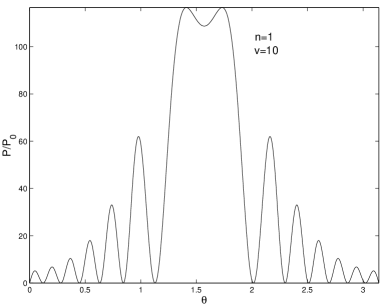
Figure 1: Angular distribution of the first harmonic of the dilaton radiation.

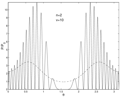
Figure 2: Second harmonic of the dilaton radiation and its averaged over ripples in terms of the MacDonald’s functions (see Eq. (47)).

where the argument of the Bessel’s functions $J_{n}$ and $J^{\prime}_{n}$ is $x=n\cos\theta$. This is shown at Figs. 1,2 for $n=1,2$ and $v=10$. Angular distribution of the first harmonic has a maximum near the equatorial plane. Oscillations are due to the interference factor $J_{0}^{2}(y)$. Recall that our assumption (25) is equivalent to $v\gg 1$, so for non-small $\theta$ one can replace $J_{0}(y)$ by the asymptotic expression (80):

$$J_{0}(y)\approx\sqrt{\frac{2}{2\pi vn\sin\theta}}\,\cos\left(2\pi vn\sin\theta-\frac{\pi}{4}\right).$$ (42)

The distribution of the second harmonic exhibits maxima displaced from the equatorial plane to some intermediate region. It is modulated by the interference factor with doubled frequency.

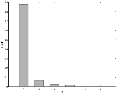
Figure 3: Distribution of the dilaton radiation over the harmonic number $n$.

Performing the angular integration one obtains the distribution over the harmonic number as shown at the Fig.3. One can see that about $88\%$ of total energy loss coresponds to the first, and about $7\%$ to the second harmonic, while the contribution from higher harmonics is relatively small.

The high frequency tail may be described using approximations for the Bessel’s functions which follow from the asymptotic formulas (74,77) valid for large $n$

$$J_{n}(na) \approx \frac{\sin\theta}{\pi\sqrt{3}}K_{1/3}\left(\frac{n}{3}\sin^{3}\theta\right),$$

$$J^{\prime}_{n}(na) \approx \frac{\sin^{2}\theta}{\pi\sqrt{3}}K_{2/3}\left(\frac{n}{3}\sin^{3}\theta\right),$$ (43)

where $K_{1/3}$ and $K_{2/3}$ are MacDonald’s functions. Since $K_{\nu}$ decrease exponentially for large values of the argument (79), it is clear that the high-frequency part of the radiation is concentrated in a narrow angular regions around $\theta=0,\,\pi$

$$\sin\theta<n^{-1/3}.$$ (44)

This beaming is a typical relativistic effect. The main contribution to the total power comes from the angular region in which the argument of the Bessel’s function $J_{0}(y)$ is large

$$y\sim 2\Omega Rn^{1/3}\gg 1,$$ (45)

so the interference factor is rapidly oscillating. Therefore one can further simplify the angular distribution for higher harmonics using the asymptotic formula (42) and averaging over the interference ripples as follows

$${\overline{J_{0}^{2}(y)}}\approx\frac{1}{\pi y}.$$ (46)

As a result, the averaged over ripples angular distribution of radiation for $n\gg 1$ will be given by the formula

$$\frac{d{\overline{P}}_{n}}{d\Omega}=\frac{4G\mu^{2}\alpha^{2}Rn}{9\pi^{2}\Omega}\sin^{7}\theta\left(K^{2}_{1/3}(z)+K^{2}_{2/3}(z)\right)^{2},$$ (47)

where

$$z=\frac{n}{3}\sin^{3}\theta.$$ (48)

Note, that this representation remains qualitatively good even for relatively small $n$, see Fig.2.

In view of a rapid convergence of the integrals from the MacDonald’s functions, we can integrate this averaged distribution over angles. Passing to the argument of the MacDonald’s functions as the new integration variable and using the relation

$$\sin^{8}\theta d\theta=\frac{9}{n^{3}}z^{2}dz,$$ (49)

where an additional factor $\sin\theta$ comes from $d\Omega$, one obtains for $n\gg 1$

$${\overline{P}}_{n}=\frac{32I_{1}G\mu^{2}\alpha^{2}R}{\pi\Omega}\,\frac{1}{n^{2}},$$ (50)

where

$$I_{1}=\int\limits\left(K^{2}_{1/3}+K^{2}_{2/3}\right)^{2}dz=4.33,$$ (51)

Therefore the contribution from high harmonics falls off as $n^{-2}$.

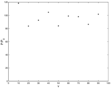
Figure 4: Total radiation power as a function of the shape parameter $v=\Omega R$.

One can also investigate the dependence of the radiated power over the shape parameter $v$ (the ratio of two radii of the torus). Numerical probes for different values of $v$ show a rather weak dependence of the total radiation power on this shape factor (see Fig.4)

V Gravitational Radiation

Gravitational radiation power can be computed along similar lines. In addition one has to distinguish between the polarisation states. The angular distribution of radiation at the frequency $\omega_{n}$ can be presented as a sum over two circular polarisations

$$\frac{dP_{n}}{d\Omega}=\frac{G\omega_{n}^{2}}{\pi}\sum_{\pm}|T^{\pm}({\bf k},\,\omega_{n})|^{2},$$ (52)

where

$$T^{\pm}({\bf k},\,\omega_{n})=\varepsilon^{\pm}_{\mu\nu}T^{\mu\nu}({\bf k},\,\omega_{n}),$$ (53)

$$T^{\mu\nu}({\bf k},\,\omega_{n})=\frac{\Omega}{\pi}\int\limits_{0}^{\pi}dt\int\limits{\rm e}^{i(\omega_{n}t-{\bf k}{\bf r})}T^{\mu\nu}({\bf r},\,t)d^{3}x.$$ (54)

Here the standard chiral graviton projectors are used

$$\varepsilon^{\pm}_{\mu\nu} = \varepsilon^{\pm}_{\mu}\varepsilon^{\pm}_{\nu},$$

$$\varepsilon^{\pm}_{\mu} = \frac{1}{\sqrt{2}}(e^{(1)}_{\mu}\pm ie^{(2)}_{\mu}),$$ (55)

where $e^{(1,2)}_{\mu}$ are two linearly independent space-like unit four-vectors orthogonal to the wave four-vector $k^{\mu}=(\omega_{n},{\bf k})$ and its spatially reflected dual ${\bar{k}}^{\mu}=(\omega_{n},-{\bf k})$,

$$e^{(1,2)}_{\mu}k^{\mu} = e^{(1,2)}_{\mu}{\bar{k}}^{\mu}=e^{(1)}_{\mu}e^{(2)\mu}=0,$$

$$e^{(1)\mu}e^{(1)}_{\mu} = e^{(2)\mu}e^{(2)}_{\mu}=-1.$$ (56)

Alternatively one could choose the linear polarisation states $e^{\oplus}_{\mu\nu},\,e^{\otimes}_{\mu\nu}$ corresponding to real and imaginary parts of (V):

$$\varepsilon^{\pm}_{\mu\nu}=\frac{1}{\sqrt{2}}\left(e^{\oplus}_{\mu\nu}\pm ie^{\otimes}_{\mu\nu}\right),$$ (57)

or, explicitly,

$$e^{\oplus}_{\mu\nu} = \frac{1}{\sqrt{2}}\left(e^{(1)}_{\mu}e^{(1)}_{\nu}-e^{(2)}_{\mu}e^{(2)}_{\nu}\right),$$

$$e^{\otimes}_{\mu\nu} = \frac{1}{\sqrt{2}}\left(e^{(1)}_{\mu}e^{(2)}_{\nu}+e^{(2)}_{\mu}e^{(1)}_{\nu}\right).$$ (58)

In the Lorentz frame in which $e^{(1,2)}_{0}=0$ two unit vectors orthogonal to ${\bf k}$ can be chosen along $\theta$ and $\varphi$ directions:

$${\bf e}^{(1)} = (\cos\theta\cos\varphi,\cos\theta\sin\varphi,-\sin\theta),$$

$${\bf e}^{(2)} = (-\sin\varphi,\cos\varphi,0).$$ (59)

As in the dilaton case, the chiral projections of the Fourier-transform of the stress tensor depend only on the difference $\sigma-\varphi$, so without loss of generality we can set $\varphi=0$. After some simplifications one finds

$$T^{\pm}({\bf k},\,\omega_{n})=\frac{\mu R}{2\pi\Omega}\int\limits_{0}^{\pi}d\chi\int\limits_{-\pi}^{-\pi}d\rho\int\limits_{0}^{2\pi}d\sigma{\rm e}^{2ni\psi}\Phi^{\pm},$$ (60)

where

$$\Phi^{\pm}=\left(\cos\sigma\cos\theta\cos\rho-\sin\theta\sin\rho\pm i\sin\sigma\cos\rho\right)^{2},$$ (61)

and $\psi$ is given again by the Eq.(36).

After the integration over $\sigma,\rho$ both chiral amplitudes lead to the same result. Indeed, purely imaginary terms in $\Phi^{\pm}$ are proportional either to $\sin 2\sigma$ or to $\sin 2\rho$; taking into account an explicit form of the phase factor $\psi$, one finds that both these terms do not contribute to the integral because of the antisymmetry of the integrand in appropriate variables. In view of the relation (57) between chiral and linear polarisation projectors this means that the gravitational radiation in any direction has only one linear polarisation component $e^{\oplus}_{\mu\nu}$. By similar reasoning one can show that the product of the first two terms in (61) also vanishes after an integration over $\rho$, so $\Phi^{\pm}$ can be replaced by the sum of the squares of each of the three terms. After some rearrangements, we find the following equivalent expression suitable for further integration

$$\Phi_{1}=\frac{\sin^{2}\theta}{4}(1-3\cos 2\rho)+\frac{1+\cos^{2}\theta}{4}\cos 2\sigma(1+\cos 2\rho).$$ (62)

Note that, contrary to the dilaton case, this function is independent on $\chi$, (i.e. on time). Therefore the integration over $\chi$ gives again the expression (IV), and the imaginary part of the integral will vanish after the integration over $\rho$; this remains true for terms in (62) containing $\cos 2\rho$. The subsequent integration over $\rho$ is performed using the integral (83). The integration over $\sigma$ directly amounts to the integral representation for the Bessel’s functions (79), and finally one obtains

$$T^{+}({\bf k},\omega_{n}) =\frac{\pi^{2}\mu R}{2\Omega}\Big{[}(1+\cos^{2}\theta)J_{2}(y)\left({J^{\prime}}_{n}^{2}-\tan^{2}\theta J_{n}^{2}\right)$$

$$+\sin^{2}\theta J_{0}(y)\left(J_{n}^{2}\left(1+3/\cos^{2}\theta\right)-3{J^{\prime}}_{n}^{2}\right)\Big{]},$$ (63)

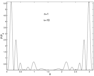
Figure 5: Angular distribution of the first harmonic the gravitonal radiation ($P_{0}=G\mu^{2}R/\Omega$)

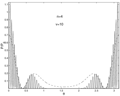
Figure 6: Angular distribution of the 4-th harmonic the gravitational radiation and its averaged approximation by MacDonald’s functions (see Eq. (64), $P_{0}=G\mu^{2}R/\Omega$.

where the argument of the Bessel’s functions of the order $n,n\pm 1$ is $x=n\cos\theta$. Now an interference of radiation produced by different parts of the membrane is accounted by two different Bessel’s functions $J_{0}(y)$ and $J_{2}(y)$; apparently this is related to the graviton spin. Since $J_{2}(0)=0$, the first term in (V) vanishes at $\theta=0,\pi$, so does the second term containing an explicit factor $\sin^{2}\theta$. Thus, contrary to the dilaton case, the amplitude of the gravitational radiation strictly along the symmetry axis is zero. Still the main part of radiation is concentrated near this direction, see Figs. 5,6.

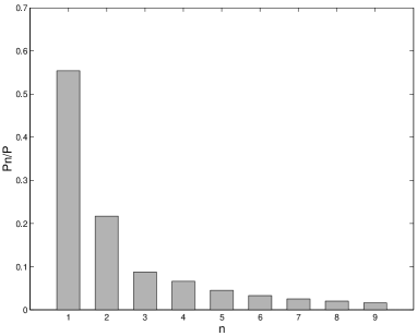
Figure 7: Distribution of the gravitational radiation over the harmonic number $n$.

The maximal contribution to the total radiation power comes from the first harmonic, but its relative contribution is smaller than in the dilaton case (Fig. 7). The high frequency tail can be described in terms of the MacDonald’s functions. For large $y$ corresponding to the main contribution to the totat power one has $J_{0}\approx J_{2}$ (see (80), this can be used before averaging over the ripples. An averaged distribution in the high frequency region is then obtained as follows

$$\frac{d{\overline{P}}_{n}}{d\Omega}=\frac{4\mu^{2}Rn}{9\pi^{2}\Omega}\sin^{7}\theta\left(3K^{2}_{1/3}(z)-K^{2}_{2/3}(z)\right)^{2}.$$ (64)

After the angular integration one gets

$${\overline{P}}_{n}=\frac{8\mu^{2}RI_{2}}{\pi\Omega}\,\,\frac{1}{n^{2}},$$ (65)

where

$$I_{2}=\int\limits\left(3K^{2}_{1/3}-K^{2}_{2/3}\right)^{2}dz=1.24.$$ (66)

This is similar to the previous result for the dilaton (47).

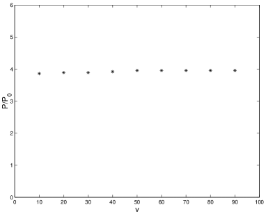
Figure 8: Total gravitational radiation power as a function of the shape parameter $v=\Omega R$.

Numerical integration for different $v$ shows that the total radiation power depends on the ratio of the torus radii even weaker than in the dilaton case (Fig. 8).

VI Concluding remarks

Let us summarize our results. We have shown that the dilaton and gravitational radiation from a vibrating relativistic membrane exhibits features typical for extended relativistic sources: the radiation power contains high harmonics of the basic frequency beamed along the symmetry axis of the torus and its angular distribution is substantially modulated due to interference. The relative contribution of the high frequency tail depends on the spin and it is more pronounced in the gravitational case. For high $n$ the averaged over ripples radiation power falls off as ${\overline{P}}_{n}\sim 1/n^{2}$ both in the dilaton and gravitational cases. The high frequency part of radiation can be conveniently described in terms of the MacDonald’s functions like in the case of ultrarelativistic point particles.

The total power of the radiation from a toroidal membrane can be presented in the form

$$P=G\mu^{2}Af(v),$$ (67)

where $A\sim Rr_{0}$ is the membrane area at the maximal extension, and the shape factor $f(v)$ is a function of the ratio of two radii of the torus (actually we observed rather weak variation of $f(v)$). On dimensional grounds it can be expected that this formula will be valid for other excitation modes up to some factor, which we set to unity $f(v)\sim 1$ for a qualitative estimate. Then in terms of the total mass of the membrane $M=\mu A$ we get

$$P\sim\frac{GM^{2}}{A},$$ (68)

so the radiative lifetime may be estimated as

$$\tau_{rad}=\frac{M}{P}\sim\frac{A}{GM}.$$ (69)

This quantity is proportional to the ratio of the area at the maximal extension to the gravitational radius of the membrane as a whole (an inverse speed of light factor has to be inserted in the ordinary units). In our model the membrane area at the moments of a maximal extension is $4\pi^{2}R/\Omega$ (recall that $\Omega$ is equal to an inverse radius of the small circle of the torus, and we assumed that $R\gg 1/\Omega$), therefore the quantity $\mu R/\Omega$ is proportional to the total mass. Thus the membrane lifetime

$$\tau\sim\frac{\mu R/\Omega}{P}\sim\frac{1}{G\mu}$$ (70)

depends only on the membrane tension. In contrary, the lifetime the radiating string loop is proportional to the loop size.

In the string case the radiative power in terms of a total mass has the order

$$P^{st}\sim\frac{GM^{2}}{L^{2}},$$ (71)

where $L$ is the string length. Correspondingly, the radiative lifetime is

$$\tau^{st}_{rad}=\frac{M}{P^{st}}\sim\frac{L^{2}}{GM}.$$ (72)

Actually our toroidal membrane has a shape of a ’thick’ string, following this similarity one can identify $L\sim R,\,A\sim Rr_{0}$. Then it is easy to see that the membrane lifetime is $R/r_{0}\gg 1$ times shorter than that of a string of an equal length.

It can be expected that gravitational radiation from membranes will depend on the membrane topology. For a toroidal membrane the radiation coming from the main excitation mode (as we have assumed here) in non-zero, while in the case of the spherical membrane the main sprerically symmetric excitation mode does not contribute to the gravitational radiation at all.

This work was supported in part by the RFBR grant 00-02-16306.

VII Appendix

Evaluating the integral in the representation of the Bessel’s functions

$$J_{n}(y)=\frac{1}{\pi}\int\limits_{0}^{\pi}\cos{(n\sigma-y\sin\sigma)}d\sigma$$ (73)

for $y=nx$ and $n\gg 1$ in the stationary phase approximation one finds

$$J_{n}(nx)\approx\frac{\sqrt{2(1-x)}}{\pi\sqrt{3}}K_{1/3}\left(\frac{2\sqrt{2}}{3}n(1-x)^{3/2}\right),$$ (74)

where $K$ is the MacDonald’s function. For the Bessel’s functions one has the following reccurent relations

$$J_{n\pm 1}(nx)=\frac{1}{x}J_{n}\mp J^{\prime}_{n},$$ (75)

while for the MacDonald’s functions with non-integer $\nu$

$$zK^{\prime}_{\nu}+\nu K_{\nu}=-zK_{1-\nu},$$ (76)

(note that $K_{-\nu}=K_{\nu}$). Differentiating (74) and using (76) one obtains in the leading approximation for large $n$ the corresponding formula for the derivative of the Bessel’s function

$$J^{\prime}_{n}(nx)\approx\frac{2(1-x)}{\pi\sqrt{3}}K_{2/3}\left(\frac{2\sqrt{2}}{3}n(1-x)^{3/2}\right).$$ (77)

For small arguments the MacDonald’s function behaves as

$$K_{\nu}(z)\sim\frac{\pi}{2\sin\pi\nu}\Gamma^{-1}(1-\nu)\left(\frac{2}{z}\right)^{\nu},$$ (78)

while for large ones

$$K_{\nu}\sim\sqrt{\frac{\pi}{2z}}{\rm e}^{-z}.$$ (79)

For Bessel’s functions at large $y$ one has

$$J_{p}(y)\approx\sqrt{\frac{2}{\pi y}}\cos\left(y-\frac{p\pi}{2}-\frac{\pi}{4}\right)$$ (80)

Passing in the Eqs.(74,77) to the limit $x\to 1$, in which case the asymptotic behavior (78) holds, one obtains for $n\gg 1$

$$J_{n}(n)\approx 3^{-2/3}\Gamma^{-1}(2/3)\left(\frac{2}{n}\right)^{1/3},$$ (81)

$${J^{\prime}}_{n}(n)\approx 3^{-1/3}\Gamma^{-1}(1/3)\left(\frac{2}{n}\right)^{2/3}.$$ (82)

In the main text we have used the following integral:

$$\int\limits_{0}^{\pi}\cos 2\mu\rho J_{2\nu}(2a\sin\rho)d\rho=\pi\cos\pi\mu J_{\nu-\mu}(a)J_{\nu+\mu}(a).$$ (83)

In particular, in view of the Eq.(75) one has

$$\int\limits_{0}^{\pi}J_{2n}(2nx\sin\rho)\cos 2\rho d\rho=\pi\left({J^{\prime}}_{n}^{2}(nx)-\frac{1}{x^{2}}J_{n}^{2}(nx)\right).$$ (84)

.

References

- (1) A. Vilenkin and E. P. S. Shellard, Cosmic strings and other topological defects. CUP, Cambridge (1992).
- (2) R. A. Battye, R. R. Caldwell and E. P. S. Shellard Gravitational waves from cosmic strings. In ”Topological defects in Cosmology”, Eds. M. Sigmore and F. Melchiori, WS, Singapore, 11-30 (1997).
- (3) T. W. B. Kibble, Topology of cosmic domain and strings. J. Phys. A9, 1387-1397 (1976).
- (4) M. B. Hindmargh and T. W. B. Kibble, Cosmic strings. Rep. Prog. Phys. 58, 477-562 (1995).
- (5) A. Vilenkin, Cosmic string and domain walls. Phys. Rept. 121, 263 (1985).
- (6) C. J. Burden, Gravitational radiation from a particular class cosmic strings. Phys. Lett. 164B, 277-281 (1985).
- (7) T. Vachaspati and A. Vilenkin, Gravitational radiation from cosmic strings. Phys. Rev D31, 3052 -3058 (1985).
- (8) D. Garfinkle and T. Vachaspati, Radiation from kinky, cuspless cosmic loops. Phys. Rev. D36, 2229 (1987).
- (9) T. Damour and A. Vilenkin, Cosmic string and the string dilaton. Phys. Rew. Lett. 78, 2288-2291 (1997).
- (10) N. Arkani-Hamed, S. Dimopoulos and G. Dvali, The hierarchy problem and new dimensions at a millimeter. Phys. Lett. B429, 263 (1998), hep-ph/9803315.
- (11) I. Antoniadis, N. Arkani-Hamed, S. Dimopoulos and G. Dvali, New dimensions at a millimeter to a Fermi and superstrings at a TeV. Phys. Lett. B436, 257 (1998), hep-ph/9804398.
- (12) P. A. Collins and R. W. Tucker, Classical and quantum mechanic free relativistic membrane. Nucl. Phys. B112, 150-176 (1976).
- (13) A. Sugamoto, Theory of membrane. Nucl. Phys. B215, 381-406 (1983).
- (14) E.D. Copeland, M. Gleiser, and H. R. Miller, Oscillous:Resonant configulations during bubble formation. Phys. Rev. D52, 1920-1933 (1995).
- (15) M. Kamionowski, A. Kosowski, and M. Turner, Gravitational radiation from first order phase transitions. Phys. Rev. D49, 2837-2851 (1994).
- (16) M. Gleiser and R. Roberts, Gravitational radiation from collapsing vacuum domains. Phys. Rev. Lett. 81, 5497-5500 (1998).
- (17) A. Kosowski, M. Turner and R. Warkins, Gravitational radiation from colliding vacuum bubbles. Phys. Rev. D45, 4514-4535 (1992).
- (18) T. Vachaspati, A. Everett and A. Vilenkin, Radiation from strings and domain walls. Phys. Rev. D30, 4525 -4535 (1992).
.