J. Math. Phys.35, 4184 (1994)
Null cone evolution of axisymmetric vacuum spacetimes

Abstract

We present the details of an algorithm for the global evolution of asymptotically flat, axisymmetric spacetimes, based upon a characteristic initial value formulation using null cones as evolution hypersurfaces. We identify a new static solution of the vacuum field equations which provides an important test bed for characteristic evolution codes. We also show how linearized solutions of the Bondi equations can be generated by solutions of the scalar wave equation, thus providing a complete set of test beds in the weak field regime. These tools are used to establish that the algorithm is second order accurate and stable, subject to a Courant-Friedrichs-Lewy condition. In addition, the numerical versions of the Bondi mass and news function, calculated at scri on a compactified grid, are shown to satisfy the Bondi mass loss equation to second order accuracy. This verifies that numerical evolution preserves the Bianchi identities. Results of numerical evolution confirm the theorem of Christodoulou and Klainerman that in vacuum, weak initial data evolve to a flat spacetime. For the class of asymptotically flat, axisymmetric vacuum spacetimes, for which no nonsingular analytic solutions are known, the algorithm provides highly accurate solutions throughout the regime in which neither caustics nor horizons form.

I Introduction

The physical basis of a new algorithm for the evolution of spacetimes has been proposed. [1] This algorithm is based upon the characteristic initial value problem for general relativity, using light cones as the evolution hypersurfaces, rather than the spacelike foliation used in traditional approaches based upon the Cauchy problem. The intimate use of characteristics has particular advantages for the description of gravitational radiation and black hole formation. [2, 3, 4]. The first attempt to carry out numerical evolution based upon this algorithm was only successful in a region outside some sufficiently large worldtube. Near the vertex of the null cone, instabilities arose which destroyed the accuracy of the code. The underlying cause of this instability was too complicated to analyze in the context of general relativity, especially since the numerical analysis of the characteristic initial value problem had not yet been carried out even for the simplest linear axisymmetric systems.

This warranted an investigation of the basic computational properties of the evolution of the flat space scalar wave equation using a null cone initial value formulation [5]. It was found that near the vertex of the cone the Courant-Friedrichs-Lewy (CFL) condition places a stricter limit on the time step than for the case of Cauchy evolution. This insight made possible the development of an extremely efficient marching algorithm for evolving the data on the initial cone by stepping it out from the vertex of the next cone to null infinity (scri) along each angular ray direction. This marching algorithm is based upon a simple identity satisfied by the values of the scalar field at the corners of a parallelogram formed by four null rays. The result was a stable, calibrated, second order accurate global algorithm on a compactified grid. Furthermore, scri played the role of a perfect absorbing boundary so that no radiation was reflected back into the system. This algorithm offers a powerful new approach to generic wave type systems. The basic idea is applicable to any of the hyperbolic systems occurring in physics.

In this paper, we apply the algorithm to the evolution of asymptotically flat, (twist-free) axisymmetric spacetimes. In a Bondi null coordinate system the metric takes the form [6]

$$ds^{2} = ({V\over r}e^{2\beta}-U^{2}r^{2}e^{2\gamma})du^{2}+2e^{2\beta}dudr+\ 2Ur^{2}e^{2\gamma}dud\theta$$ (2)

$$-r^{2}(e^{2\gamma}d\theta^{2}+e^{-2\gamma}\sin^{2}\theta d\phi^{2}).$$

The vacuum field equations then decompose into the three hypersurface equations

$$\beta_{,r}=\frac{1}{2}r\>(\gamma_{,r})^{2}$$ (3)

$$[r^{4}\,e^{2(\gamma-\beta)}U_{,r}]_{,r}=2r^{2}[r^{2}(\frac{\beta}{r^{2}})_{,r\theta}-\frac{(\sin^{2}\theta\,\gamma)_{,r\theta}}{\sin^{2}\theta}+2\,\gamma_{,r}\,\gamma_{,\theta})]$$ (4)

$$V_{,r} = -\frac{1}{4}r^{4}e^{2(\gamma-\beta)}(U_{,r})^{2}+\frac{(r^{4}\sin\theta U)_{,r\theta}}{2r^{2}\sin\theta}$$ (6)

$$+e^{2(\beta-\gamma)}[1-\frac{(\sin\theta\beta_{,\theta})_{,\theta}}{\sin\theta}+\gamma_{,\theta\theta}+3\cot\theta\gamma_{,\theta}-(\beta_{,\theta})^{2}-2\gamma_{,\theta}(\gamma_{,\theta}-\beta_{,\theta})]$$

and one evolution equation

$$4r(r\gamma)_{,ur} = [2r\gamma_{,r}V-r^{2}(2\gamma_{,\theta}\,U+\sin\theta({U\over{\sin\theta}})_{,\theta})]_{,r}-2r^{2}\frac{(\gamma_{,r}U\sin\theta)_{,\theta}}{\sin\theta}$$ (8)

$$+\frac{1}{2}r^{4}e^{2(\gamma-\beta)}(U_{,r})^{2}+2e^{2(\beta-\gamma)}[(\beta_{,\theta})^{2}+\sin\theta({\beta_{,\theta}\over{\sin\theta}})_{,\theta}].$$

The initial data consists of $\gamma$, which is unconstrained except by smoothness conditions. Because $\gamma$ represents a spin-2 field, it must be $O(\sin^{2}\theta)$ near the axis and consist of $l\geq 2$ spin-2 multipoles.

Here we are interested in the global application of this system when the null hypersurfaces are null cones, although the approach also goes through without major change if the null hypersurfaces emanate from a finite world tube. We require that the null cones have nonsingular vertices which trace out a geodesic worldline $r=0$. For the quadrupole terms, this implies the boundary conditions $\gamma=O(r^{2})$, $\beta=O(r^{4})$, $U=O(r)$ and $V=r+O(r^{3})$. For higher multipoles, the smoothness conditions can be worked out by referring back to local Minkowski coordinates [7]. As a consequence, $O({r^{n}})$ terms in $\gamma$ can contain multipoles with $2\leq l\leq n$. Any satisfactory computational algorithm must meet the challenge of preserving these smoothness conditions.

In Sec. II, we analyze the linearized version of these equations and show how their solutions may be obtained locally from solutions of the scalar wave equation. This provides an important means of constructing linearized solutions in a null cone gauge for the purpose of code calibration. It also reveals essential changes in the grid structure necessary in adapting the null parallelogram algorithm for the wave equation to linearized gravity.

This also solves the major computational problems for the nonlinear case. In Sec. III, we show how the linearized algorithm can be extended to this case. In Sec. IV, we discuss the major finite difference techniques necessary for second order accuracy. In Sec. V, we present a study of the stability and accuracy of an evolution code based upon this algorithm. New exact and linearized solutions are introduced to establish second order convergence. In addition, a global check on accuracy is carried out using Bondi’s formula relating mass loss to the time integral of the square of the news function.

II The Linearized Bondi Equations

In the linearized limit $\beta=0$ and $V=r$. The equations (3)-(8) reduce to one hypersurface equation and one evolution equation for the surviving field variables $\gamma$ and $U$,

$$(r^{4}U_{,r})_{,r}=-\frac{2r^{2}(\sin^{2}\theta\,\gamma)_{,r\theta}}{\sin^{2}\theta}$$ (9)

$$4r(r\gamma)_{,ur}=[2r^{2}\gamma_{,r}-r^{2}\sin\theta({U\over{\sin\theta}})_{,\theta}]_{,r}.$$ (10)

Physical considerations suggest that these equations be related to the wave equation. If this relationship were sufficiently simple, then the scalar wave algorithm could be used as a guide in formulating an algorithm for evolving $\gamma$. A scheme for generating solutions to the linearized Bondi equations in terms of solutions to the wave equation has been presented previously [6]. However, in that scheme, the relationship of the scalar wave to $\gamma$ is non-local in the angular directions and is not useful for this purpose.

We now formulate an alternative scheme in terms of spin-weight 0 quantities $\alpha$ and $Z$, related to $\gamma$ (spin-weight 2) and $U$ (spin-weight 1) by [8]

$$\gamma=\eth^{2}\alpha=\sin\theta\partial_{\theta}({1\over{\sin\theta}}\partial_{\theta}\alpha)$$ (11)

$$U=\eth Z=\partial_{\theta}Z.$$ (12)

Then the linearized equations are equivalent to

$$(r^{4}Z_{,r})_{,r}=-2r^{2}(2-L^{2})\alpha_{,r},$$ (13)

and

$$E:=2(r\alpha)_{,ur}-r^{-1}(r^{2}\alpha_{,r}-r^{2}Z/2)_{,r}=0,$$ (14)

where $L^{2}=-(1/\sin\theta)\partial_{\theta}(\sin\theta\partial_{\theta})$ is the $\theta$-part of the angular momentum operator. Now let $\Phi$ be a solution of the flat space scalar wave equation,

$$r\Box\,\Phi=2(r\Phi)_{,ur}-(r\Phi)_{,rr}+r^{-1}L^{2}\Phi=0,$$ (15)

and set

$$r^{2}\alpha_{,r}=(r^{2}\Phi)_{,r}$$ (16)

and

$$r^{2}Z_{,r}=2(L^{2}-2)\Phi.$$ (17)

Then

$$E=r\Box\,\Phi+2(\Phi+\alpha)_{,u}-2r^{-2}(r^{2}\Phi)_{,r}+Z,$$ (18)

and

$$E_{,r}=r^{-2}(r^{3}\Box\,\Phi)_{,r}$$ (19)

Equation (13) is satisfied as a result of (16) and (17)and the wave equation (15) implies $E_{,r}=0$. If $\Phi$ is smooth and $O(r^{2})$ at the origin, this implies $E=0$, so that the linearized equations are satisfied. The condition that $\Phi=O(r^{2})$ eliminates fields with only monopole and dipole dependence so that it does not restrict the generality of the spin-weight 2 function $\gamma$ obtained through (11).

Thus for any linearized axisymmetric gravitational wave in the null cone gauge, $\gamma$ may be related to a scalar wave by (11) and (16). The CFL condition for convergence of a finite difference algorithm requires that the numerical domain of dependence be larger than the physical domain of dependence. Because the relationship between $\Phi$ and $\gamma$ is local with respect to the null rays on the cone, their domains of dependence coincide. This suggests that a stable and convergent evolution algorithm for the gravitational field may be modeled upon the scalar wave algorithm. This turns out to be the case although some subtle distinctions arise, as described below.

An evolution algorithm for scalar waves has been formulated in terms of an integral identity for the values of the field at the corners of a null parallelogram lying on the $(u,r)$ plane [5]. The wave equation with source, $\Box\Phi=S$, can be reexpressed in the form

$$\Box\,^{(2)}\psi=-{L^{2}\psi\over r^{2}}+rS,$$ (20)

where $\psi=r\Phi$ and $\Box\,^{(2)}$ is the 2-dimensional wave operator intrinsic to the $(u,r)$ plane. Integration over the null parallelogram as depicted in Fig. 1 then leads to the integral equation

$$\psi_{Q}=\psi_{P}+\psi_{S}-\psi_{R}+{1\over 2}\int_{A}dudr[-{L^{2}\psi\over r^{2}}+rS],$$ (21)

where $P$, $Q$, $R$ and $S$ are the corners and $A$ the area of the parallelogram.

This identity gives rise to an explicit marching algorithm for evolution. Let the null parallelogram span null cones at adjacent grid values $u_{0}$ and $u_{0}+\Delta u$, as shown in Fig. 1, for some $\theta$ and $\phi$. If $\psi$ has been determined on the entire $u_{0}$ cone and on the $u_{0}+\Delta u$ cone radially outward from the origin to the point $P$, then (21) determines $\psi$ at the next point $Q$ in terms of an integral over $A$. This procedure can then be repeated to determine $\psi$ at the next radially outward point $T$ in Fig. 1. After completing this radial march to scri, the field $\psi$ is then evaluated on the next null cone at $u_{0}+2\Delta u$, beginning at the vertex where smoothness gives the start up condition that $\psi=0$. The resulting evolution algorithm is a 2-level scheme which reflects, in a natural way, the distinction between characteristic and Cauchy evolution, i.e. that the time derivative of the field is not part of the characteristic initial data.

The CFL condition on the numerical domain of dependence is a necessary condition for convergence of a numerical algorithm. For the grid point at $(u,r,\theta)$, there are three critical grid points, $(u-\Delta u,r+\Delta r,\theta)$ and $(u-\Delta u,r-\Delta r,\theta\pm\Delta\theta)$, which must lie inside its past physical light cone. These gives rise to the inequalities $\Delta u<2\Delta r$ and $\Delta u<-\Delta r+(\Delta r^{2}+r^{2}\Delta\theta^{2})^{1/2}$. At large $r$, the second inequality becomes $\Delta u<r\Delta\theta$ and the limitations on the time step are essentially the same as for a Cauchy evolution algorithm. However, near the vertex of the cone, the second inequality gives a stricter condition

$$\Delta u<K\Delta r\Delta\theta^{2},$$ (22)

where $K$ is a number of order $1$ whose exact value depends upon the start up details at the vertex. For the scalar wave equation, these stability limits were confirmed by numerical experimentation and it was found [5] that $K\approx 4$.

The linearized gravitational evolution equation (10) can be recast into a form similar to (20),

$$\Box\,^{(2)}\psi={\cal H},$$ (23)

where now $\psi=r\gamma$ and ${\cal H}$ only contains hypersurface terms. This allows use of the null parallelogram algorithm to evolve $\gamma$ by the same marching scheme as in the scalar case. The additional feature here is that $U$ must be simultaneously marched out the null cone using the hypersurface equation (9). For the scalar wave equation (20), the angular momentum barrier is represented by the term $L^{2}\psi/r^{2}$, which is determined from $\psi$ by a double angular derivative. In the linearized gravitational evolution equation (10), the analogous term is $[r^{2}\sin\theta({U/\sin\theta})_{,\theta}]_{,r}$, which is determined from $U$ by a single angular derivative. In turn, the hypersurface equation (9) relates $U$ to $\gamma$ by a single angular derivative. Physically, this has the same net effect of producing an angular momentum barrier depending upon the second angular derivative, as in the scalar case. However, the nontrivial mathematical distinction between the two cases leads to nontrivial difference in their natural grid structures for a numerical algorithm. In particular, the grid for $U$ must be staggered between the grid points for $\gamma$. These and other details of the marching algorithm will be given in Sec. IV, where we discuss the nonlinear case.

The use of scalar waves to generate solutions of the linearized Bondi equations provides an important tool for testing evolution algorithms in the linear regime. Monopole solutions may be represented in the form $\Phi=[F(u+2r)-F(u)]/r$ and axisymmetric multipoles may be built up by applying the $z$-translation operator

$$\partial_{z}=\cos\theta(\partial_{r}-\partial_{u})-r^{-1}\sin\theta\partial_{\theta}$$ (24)

to these solutions. Then $\gamma$ may be obtained via (11). For the calibration measurements in Sec. V, we use the solutions

$$\Phi=(\partial_{z})^{\ell}[u(u+2r)]^{-1},$$ (25)

obtained by applying $(\partial_{z})^{\ell}$ to the fundamental Lorentz invariant solution $1/(x^{\alpha}x_{\alpha})$. This solution is well behaved above the singular light cone $u=0$.

III The Nonlinear Algorithm

The nonlinear evolution equation (8) can also be recast in the form of (23) in terms of $\psi=r\gamma$, for an appropriate choice of 2-dimensional wave operator $\Box\,^{(2)}$. In this case, the $(u,r)$ submanifold is not flat so that it would not be appropriate to base $\Box\,^{(2)}$ upon a flat metric. Indeed, such a choice would lead to an improper domain of dependence and could not be used as the basis for a stable algorithm. It would seem more natural to use the $\Box\,^{(2)}$ operator of the metric induced in the $(u,r)$ submanifold by the 4-dimensional metric (2). Here we pursue an alternative choice based upon the line element

$$d\sigma^{2}=2l_{(\mu}n_{\nu)}=e^{2\beta}du[\frac{V}{r}du+2dr],$$ (26)

where $l_{\mu}=u_{,\mu}$ is the normal to the outgoing null cones and $n_{\mu}$ is the other null vector normal to the spheres of constant $r$. Although this choice is not unique and other possibilities deserve exploration, it leads to the simplest ${\cal H}$-terms when reexpressing (8) in the form (23). Because the domain of dependence of $d\sigma^{2}$ contains the domain of dependence of the induced metric of the $(u,r)$ submanifold, this approach does not lead to convergence problems associated with the CFL condition.

The wave operator associated with (26) is

$$\Box\,^{(2)}\psi=e^{-2\beta}[2\psi_{,ru}-(\frac{V}{r}\psi_{,r})_{,r}]$$ (27)

and the nonlinear evolution equation (8) becomes

$$\Box\,^{(2)}\psi=e^{-2\beta}{\cal H},$$ (28)

where

$${\cal H} = -({V\over r})_{,r}\gamma-{1\over r}[r^{2}(\gamma_{,\theta}U+\frac{1}{2}\sin\theta({U\over{\sin\theta}})_{,\theta})]_{,r}$$ (31)

$$-r\frac{(\gamma_{,r}U\sin\theta)_{,\theta}}{\sin\theta}+\frac{1}{4}r^{3}e^{2(\gamma-\beta)}(U_{,r})^{2}$$

$$+{1\over r}e^{2(\beta-\gamma)}[(\beta_{,\theta})^{2}+\sin\theta({\beta_{,\theta}\over{\sin\theta}})_{,\theta}].$$

Because all 2-dimensional wave operators are conformally flat, with conformal weight $-2$, the surface integral of (28) over a null parallelogram gives an integral equation analogous to (21),

$$\psi_{Q}=\psi_{P}+\psi_{S}-\psi_{R}+{1\over 2}\int_{A}du\,dr{\cal H}.$$ (32)

This allows the evolution of $\gamma$ by the same basic marching algorithm as described in Sec. II for the scalar wave and linearized wave cases. The additional modifications are that $\beta$, $U$, and $V$ must be simultaneously marched out the null cone using the nonlinear hypersurface equations (3)-(6). Because of the hierarchal structure of these equations, $\gamma$, $\beta$, $U$, and $V$ may be marched in that order without any matrix inversions or other implicit operations. The basic computational cell and finite difference constructions are described in the next section.

Near the origin, the metric approaches the Minkowski metric so that the stability of the nonlinear algorithm in this region should be subject to the same Courant limit as for the linearized equations. Near scri, the gravitational variables have the asymptotic form

$$\gamma = K+r^{-1}c+O(r^{-2})$$ (33)

$$\beta = H+O(r^{-2})$$ (34)

$$U = L+O(r^{-1})$$ (35)

$$V = r^{2}{(L\sin\theta)_{,\theta}\over{\sin\theta}}$$ (36)

$$+ re^{2(H-K)}\Big{[}1+2{(H_{,\theta}\sin\theta)_{,\theta}\over{\sin\theta}}+{(K_{,\theta}\sin^{3}\theta)_{,\theta}\over{\sin^{3}\theta}}+4(H_{,\theta})^{2}-4H_{,\theta}K_{,\theta}-2(K_{,\theta})^{2}\Big{]}$$ (37)

$$- 2e^{2H}{\cal M}+O(r^{-1}),$$ (38)

where ${\cal M}$ corresponds to Bondi’s mass aspect. In a standard Bondi frame at scri $K$, $H$, and $L$ all vanish, but not in null cone coordinates adapted to a Minkowski frame at the origin. This dependence can lead to drastic behavior of the $u$-coordinate at large distances. In a numerical study of spherically symmetric, self-gravitating scalar radiation fields [2], $H\rightarrow\infty$ as a horizon is formed and an infinite redshift develops between central observers and observers at scri. In that case, a consideration of the domains of dependence indicates that the step size $\Delta u$ for stable evolution must approach zero as the horizon is formed. The divergence of the outgoing null cone equals $e^{-2\beta}/r$. If $\beta\rightarrow\infty$ at a finite value of $r$ then a caustic will in general form. When this occurs, a single null cone coordinate system cannot cover the entire exterior region of the spacetime.

In the more general case being considered here, it is also possible for the $u$-direction to become spacelike at large distances, corresponding to the coefficient of $du^{2}$ in (2) becoming negative. (The $u=constant$ hypersurfaces, of course, must remain null.) As discussed in Sec. V, this does not affect the stability of the algorithm. The algorithm is also valid when the vertex of the null cone is replaced by an inner boundary consisting of a timelike or null worldtube, so that it may also be applied to other versions of the characteristic initial value problem [9].

IV Finite Difference Techniques

The numerical grid is based upon the outgoing null cones, using the compactified radial coordinate $x=r/(1+r)$ and the angular coordinate $y=-\cos\theta$. Thus points at scri are included in the grid at $x=1$.

In order to improve numerical accuracy at the grid boundaries, the code is written in terms of the variables $\hat{\psi}=r\hat{\gamma}=r{\gamma}/\sin^{2}\theta$, $\beta$, $S=(V-r)/r^{2}$ and $\hat{U}=U/\sin\theta$. For a pure quadrupole mode, $\hat{\gamma}$ has constant angular dependence.

To develop a discrete evolution algorithm, we work with two sets of spatial grid points, both of which have the constant spacing $\Delta x=1/N_{x}$ and $\Delta y=1/N_{y}$. The first grid is defined by $(u^{n},x_{i},y_{j})=(n\Delta u,i\Delta x,j\Delta y)$. The second grid is shifted (staggered) in both the $x$ and $y$ variables and is thus defined by $(u^{n},x_{i+\frac{1}{2}},y_{j+\frac{1}{2}})=(n\Delta u,(i+\frac{1}{2})\Delta x,(j+\frac{1}{2})\Delta y)$. Note that the staggered grid extends beyond the physical boundary $x=1$. This peculiarity is successfully exploited for a smooth calculation of the metric at scri. The time step is variable and is limited by the largest possible value that would satisfy the CFL condition over the entire grid.

A staggerered grid is not necessary for the scalar wave equation but its introduction for the gravitational case is dictated by a detailed von Neumann stability analysis of the linearized equations. Accordingly, $\hat{\gamma},\beta\,\mbox{and}\,\,S$ reside on the $(x_{i},y_{j})$ grid while $\hat{U}$ is placed on the $(x_{i+\frac{1}{2}},y_{j+\frac{1}{2}})$ grid. We denote values of a field $F$ at the site $(n,i,j)$ by $F^{n}_{ij}=F(u^{n},x_{i},y_{j})$. We use centered second order differences for derivatives at points not on the edges of the grid, e.g. for an arbitrary field $F$

$${F_{,y|}}_{i,j}={1\over{2\Delta y}}(F_{i,j+1}-F_{i,j-1})$$ (39)

To calculate derivatives of the field at the edges of the grid, we use backward and forward second-order differences, e.g at the $y=\pm 1$ edges of the grid, where $j=\pm N_{y}$

$${F_{,y|}}_{i,\pm N_{y}}=\mp{1\over{2\Delta y}}(-F_{i,\pm N_{y}\mp 2}+4F_{i,\pm N_{y}\mp 1}-3F_{i,\pm N_{y}})$$ (40)

A The Hypersurface Equations

In terms of the numerical variables $\hat{\gamma}$, $\beta$, $S$ and $\hat{U}$, and expressed in the coordinates $x$ and $y$ used in the code, the hypersurface equations (3)-(6) are

$$\beta_{,x} = {\cal H}_{\beta}$$ (41)

$$({x^{4}\over(1-x)^{2}}\,e^{2((1-y^{2})\hat{\gamma}-\beta)}{\hat{U}}_{,x})_{,x} = 2{x^{2}\over(1-x)^{2}}\>{\cal H}_{U}$$ (42)

$$x^{2}S_{,x}+{{2x}\over{1-x}}S = {\cal H}_{S},$$ (43)

where the source terms ${\cal H}_{\beta}$, ${\cal H}_{U}$ and ${\cal H}_{S}$ are given by

$${\cal H}_{\beta} = \frac{1}{2}x(1-x)(1-y^{2})^{2}\>(\hat{\gamma}_{,x})^{2}$$ (44)

$${\cal H}_{U} = \beta_{,xy}-{2\over{x(1-x)}}\beta_{,y}+4y\hat{\gamma}_{,x}+(1-y^{2})[2\hat{\gamma}_{,x}((1-y^{2})\hat{\gamma}_{,y}-2y\hat{\gamma})-\hat{\gamma}_{,xy}]$$ (45)

$${\cal H}_{S} = -1-xy[{4\over{1-x}}{\hat{U}}+x{\hat{U}}_{,x}]+{1\over 2}(1-y^{2})x[{4\over{1-x}}{\hat{U}}_{,y}+x{\hat{U}}_{,xy}]$$ (49)

$$-{1\over 4}x^{4}({\hat{U}}_{,x})^{2}(1-y^{2})e^{2((1-y^{2})\hat{\gamma})-\beta}-e^{2(\beta-(1-y^{2})\hat{\gamma})}\{-1-12\hat{\gamma}-2y\beta_{,y}$$

$$+(1-y^{2})[10\hat{\gamma}+8y\hat{\gamma}_{,y}+8\hat{\gamma}^{2}+4y\hat{\gamma}\beta_{,y}+\beta_{,yy}+(\beta_{,y})^{2}$$

$$-(1-y^{2})^{2}(8\hat{\gamma}^{2}+2\hat{\gamma}_{,y}\beta_{,y}+\hat{\gamma}_{,yy}+8y\hat{\gamma}\hat{\gamma}_{,y})+2(1-y^{2})^{3}(\hat{\gamma}_{,y})^{2}\}.$$

Note that Eq. (41) has just one radial derivative, and can be evaluated at the points $(n,i-\frac{1}{2},j)$. We can discretize it as follows

$$\beta_{i,j}=\beta_{i-1,j}+({\cal H}_{\beta})_{i-\frac{1}{2},j}\,\Delta x.$$ (50)

Equation (42), which contains a second radial derivative, is evaluated at the points $(n,i-1,j)$. Near the origin, where $\hat{U}=O(x)$, it becomes a singular differential equation. In order to integrate it to second order accuracy it is necessary to apply numerical regularization to the derivatives on the left hand side. Noting that $\partial/\partial x=4x^{3}\partial/\partial x^{4}$, Eq. (42) becomes

$$2x(1-x)[x^{4}{\hat{U}}_{x}]_{,x^{4}} + x^{2}[1-(1-x)(\beta_{,x}-(1-y^{2})\hat{\gamma}_{,x})]{\hat{U}}_{,x}$$ (51)

$$= e^{2(\beta-(1-y^{2})\hat{\gamma})}(1-x){\cal H}_{U}.$$ (52)

Using the identity

$$x^{4}_{i-\frac{1}{2}}-x^{4}_{i-1-\frac{1}{2}}=2\Delta x\,x_{i-1}(x^{2}_{i-\frac{1}{2}}+x^{2}_{i-1-\frac{1}{2}}),$$ (53)

we can discretize (52) as

$${(1-x_{i-1})\over{(x^{2}_{i-\frac{1}{2}}+x^{2}_{i-1-\frac{1}{2}})}}[x^{4}_{i-\frac{1}{2}}({\hat{U}}_{i,j}-{\hat{U}}_{i-1,j})-x^{4}_{i-1-\frac{1}{2}}({\hat{U}}_{i-1,j}-{\hat{U}}_{i-2,j})]$$ (54)

$$+ {1\over 2}x^{2}_{i-1}\Delta x[1-(1-x_{i-1})(\beta_{i,j}-\beta_{i-2,j}-(1-y^{2}_{j})(\hat{\gamma}_{i,j}-\hat{\gamma}_{i-2,j})){1\over{\Delta x}}]({\hat{U}}_{i,j}-{\hat{U}}_{i-2,j})$$ (55)

$$= (\Delta x)^{2}(1-x_{i-1})\>({\cal H}_{U})_{i-1,j}.$$ (56)

The above is a 3-point formula, and it can not be applied at the points at $x_{i}=\Delta x$, however we know the asymptotic behavior of $U$ at the origin, and we can use it to construct a starting algorithm for these points. We approximate the Bondi equations for $\hat{\gamma}$ and $\hat{U}$ by the leading two terms in a power series,

$$\hat{\gamma} = ar^{2}+br^{3}$$ (57)

$$\hat{U} = 4y(ar+\frac{1}{3}br^{2}),$$ (58)

Expanding $\hat{\gamma}_{,u}$ to the same order, we obtain for the rate of change of $a$ and $b$

$$a_{,u} = \frac{6}{5}b$$ (59)

$$b_{,u} = 0.$$ (60)

By fitting a least square polynomial to $\hat{\gamma}/r^{2}$ near the origin, we can read off the coefficients $a$ and $b$ and evaluate $\hat{U}$ on the next hypersurface. This approximation is consistent with the global second order accuracy of the algorithm.

As with Eq. (41), Eq. (43) can be approximated at sites $(n,i-\frac{1}{2},j)$ as follows

$$x^{2}_{i-\frac{1}{2}}{1\over{\Delta x}}(S_{i,j}-S_{i-1,j}) + {x_{i-\frac{1}{2}}\over{1-x_{i-\frac{1}{2}}}}(S_{i,j}+S_{i-1,j})$$ (61)

$$= ({\cal H}_{S})_{i-\frac{1}{2},j}.$$ (62)

B The Evolution Equation

In practice, the corners of the null parallelogram, $P$, $Q$, $R$ and $S$, cannot be chosen to lie exactly on the grid because the velocity of light in terms of the compactified coordinate $x$ is not constant even in flat space. Numerical experimentation suggests that a stable algorithm with high accuracy results from the choice made in Fig. 1. The essential feature of this placement of the parallelogram with respect to a coordinate cell is that the sides formed by incoming rays intersect adjacent u-hypersurfaces at equal but opposite x-displacements from the neighboring grid points. Solution for the null geodesics of the metric (26) to second order accuracy then gives for the coordinates of the vertices

$$x_{i-1}-x_{P} = x_{R}-x_{i-1}$$ (63)

$$= \Delta u(1-x_{i-1})^{2}[1+r_{i-1}(S^{n+1}_{i-2}+S^{n}_{i})/2]/4$$ (64)

$$x_{i}-x_{Q} = x_{S}-x_{i}$$ (65)

$$= \Delta u(1-x_{i})^{2}[1+r_{i}(S^{n+1}_{i-1}+S^{n}_{i+1})/2]/4.$$ (66)

The elementary computational cell consists of the lattice points $(n,i,j)$ and $(n,i\pm 1,j)$ on the “old” hypersurface and the points $(n+1,i-2,j)$, $(n+1,i-1,j)$ and $(n+1,i,j)$ on the “new” hypersurface (and their nearest neighbors in the angular direction). The marching algorithm computes the value of the fields at the point $(n+1,i,j)$ in terms of their predetermined values at the other points in the cell.

The values of $\hat{\psi}$ at the vertices of the parallelogram are approximated to second order accuracy by linear interpolation between grid points. Furthermore, cancellations arise between these four interpolations so that the evolution equation (32) is satisfied to fourth order accuracy, provided the integral can be calculated to that accuracy. This is accomplished by approximating the integrand by its value at the center of the parallelogram. To second order accuracy, this gives

$$\int_{A}du\,dr\,{\cal H}={\cal H}_{c}\,\int_{A}du\,dr=\frac{1}{2}\Delta u\,(r_{Q}-r_{P}+r_{S}-r_{R}){\cal H}_{c},$$ (67)

where the centered value ${\cal H}_{c}$ can be obtained by averaging between appropriate points in the cell. Thus the discretized version of (32) is given by

$$\hat{\psi}^{n+1}_{i} = {\cal F}(\hat{\psi}^{n+1}_{i-1},\hat{\psi}^{n+1}_{i-2},\hat{\psi}^{n}_{i+1},\hat{\psi}^{n}_{i},\hat{\psi}^{n}_{i-1})$$ (69)

$$+\frac{1}{2}\Delta u\,(r_{Q}-r_{P}+r_{S}-r_{R}){\cal H}_{c}$$

where ${\cal F}$ is a linear function of $\psi$ and the $j$ index has been suppressed.

Consequently, it is possible to move through the interior of the lattice, computing $\hat{\psi}^{n+1}_{i}$ explicitly by an orderly radial march. This is achieved by starting at the origin at time $u^{n+1}$. Field values vanish there. Next, proceed outward one radial step using the boundary conditions (discussed below). Then step outward to the next interior radial point using (69), iterating this process throughout the interior and for all angles. This updates all field values stretching to scri along the new null cone at $u^{n+1}$, thus completing one evolutionary time step.

The above scheme is sufficient for accurate evolution in a neighborhood of the origin. Global evolution, including the points at $x=1$, requires careful manipulation of (69) to avoid problems from the fact that $\psi\sim rK$ at scri. Thus the direct use of this formula is not possible for the point at scri, while points near scri would suffer serious loss of accuracy. We renormalize (69) in the following way. First, we introduce the quantity $\phi=\psi(1-x)$. Near scri $\phi$ has the desired finite behavior, while near the origin it leaves unchanged the constant coefficient form of the evolution equation, thus preserving the stability properties. With this substitution and with the use of (67), the evolution equation (32) becomes

$$\phi_{Q} = {1\over 4}\Delta u\,x_{Q}{\cal H}_{c}+\frac{(1-x_{Q})}{(1-x_{P})}(\phi_{P}-{1\over 4}\Delta u\,x_{P}{\cal H}_{c})$$ (71)

$$+\frac{(1-x_{Q})}{(1-x_{S})}(\phi_{S}+{1\over 4}\Delta u\,x_{S}{\cal H}_{c})-\frac{(1-x_{Q})}{(1-x_{R})}(\psi_{R}+{1\over 4}\Delta u\,x_{R}{\cal H}_{c})$$

Now all terms have finite asymptotic value. The coefficient $(1-x_{Q})/(1-x_{S})$ has $0/0$ behavior at scri but approaches the limit $1$. Further refinement is possible with the use of the explicit second order approximation for the characteristics (66) which leads to the approximation

$$\frac{(1-x_{Q})}{(1-x_{S})}=1+2\frac{\delta}{1-\delta}$$ (72)

where

$$\delta={1\over 4}\Delta u(1+x_{i}(S^{n+1}_{i-1}+S^{n}_{i+1})/2)$$ (73)

The final result is that the equation (71) propagates $\phi$ radially outward one cell with an error of fourth order in grid size. This is valid for all interior points and the point at scri. The error in each cell compounds to a third order error on each null cone and a second order global error after evolving for a given physical time. Second order global accuracy is indeed confirmed by the convergence tests described in Sec. V.

We mentioned that a modified form of the basic grid cell Eq. (66) is used at the origin. This is necessary since the incoming characteristic through the points $P$ and $R$ can not be centered at $x=0$. The corners of the modified cell are given by

$$x_{P} = 0$$ (74)

$$x_{R} = \frac{1}{2}\Delta u$$ (75)

$$x_{1}-x_{Q} = x_{S}-x_{1}=\frac{1}{4}\Delta u(1-x_{i})^{2}.$$ (76)

Only the linear terms of ${\cal H}$ are kept while evolving the first point, i.e. for $x_{1}=\Delta x$. This reduces equation (32) to

$$\hat{\psi}_{Q}=\hat{\psi}_{S}-\hat{\psi}_{R}-{1\over 4}\int_{A}du\,dr\frac{1}{r}(r^{2}\hat{U}_{,y})_{,r}.$$ (77)

Using the expansion (58) for $U$ near the origin, the integral simplifies further to

$$\int_{A}du\,dr(3\,a\,r+\frac{12}{5}\,b\,r^{2}).$$ (78)

The integrand is now evaluated to second order accuracy at $u^{n+\frac{1}{2}}=u^{n}+\frac{\Delta u}{2}$ using

$$a^{n+\frac{1}{2}}=a^{n}+\frac{6}{5}b^{n}\frac{\Delta u}{2}$$

and $b^{n+\frac{1}{2}}=b^{n}$. Keeping higher order terms would not improve the global convergence rate of the code.

V Code tests

A Testbeds

As we have shown in Sec. II, linearized solutions of the Bondi equations can be generated by solutions of the scalar wave equation, thus supplying a complete set of test beds for the very weak regime. For the nonlinear case, exact boost and rotation symmetric solutions [10] of the Bondi initial hypersurface equations have also been found [11]. They have been used to check the radial integrations leading from $\gamma$ to $\beta$, $U$ and $V$ but they do not provide a test of the evolution algorithm. However, in the course of this work, we have found that one of these initial data sets is in fact preserved under time evolution and is an exact static solution of the nonlinear vacuum equations.

This solution provides an important test bed for null cone evolution codes. Except for spherically symmetric cases, it is the only known solution of Einstein’s equation which can be expressed explicitly in null cone coordinates with no singularity at the vertex. It has the form

$$2\>e^{\gamma} = 1+\Sigma$$ (79)

$$e^{2\beta} = {(1+\Sigma)^{2}\over{4\Sigma}}$$ (80)

$$U = -{{a^{2}\rho\>\sqrt{r^{2}-\rho^{2}}}\over{r\>\Sigma}}$$ (81)

$$V = {{r\>\left(2\>a^{2}\rho^{2}-a^{2}\>r^{2}+1\right)}\over{\Sigma}}$$ (82)

where $\rho=r\sin\theta$, $\Sigma=\sqrt{1+a^{2}\rho^{2}}$ and $a$ is a free scale parameter. It is remarkable that the null data $\gamma$ is time independent under evolution, as can be verified by inserting the above expressions in (8). Because this solution is static, as well as boost and rotation symmetric, the commutator between the boost and time translation symmetries implies that it has an additional translation symmetry in the boost direction. Thus the solution falls into several overlapping and widely studied classes, including the static cylindrically symmetric spacetimes and the Weyl static axisymmetric spacetimes. However, this solution, which we call SIMPLE, has not previously been singled out, apparently because it cannot easily be identified in the traditional coordinates used for studying static solutions. Because of its cylindrical symmetry, it is clear that this solution is not asymptotically flat but it can be used to construct an asymptotically flat, nonsingular solution by smoothly pasting asymptotically flat null data to it outside some radius $R$. The resulting solution will be static and given by (82) in the domain of dependence interior to $R$. Numerical solutions generated by this technique are used in the code calibration tests presented below.

In addition, global energy conservation provides an important test bed. The Bondi mass loss formula is not one of the equations used in the evolution algorithm but follows from those equations as a consequence of a global integration of the Bianchi identities.

B Convergence and Stability

We have tested the algorithm to be second order accurate and stable, subject to the CFL condition, throughout the regime in which caustics and horizons do not form. In Sec. II, we showed how the the linearized Bondi equations may be reduced to the scalar wave equation by local operations. For very weak data, the nonlinear equations approximate the linear equations so that we would expect the global stability of the nonlinear algorithm to be related to the CFL condition for the scalar wave algorithm. Near the origin, stability checks show that the time step is limited by (22) with $K=8$, which is twice the limit found for the scalar wave algorithm. This factor of two apparently arises from the use of a staggered grid in the gravitational case, which effectively doubles the value of $r$ at which the main algorithm takes over from the start up algorithm at the origin. This gives some reassurance that the scalar wave algorithm has been optimally adapted to the Bondi equations.

By construction, the $u$-direction is timelike at the origin where it coincides with the worldline traced out by the vertex of the outgoing null cone. But even for weak fields, the $u$-direction becomes spacelike at large distances along a typical outgoing ray. This can be seen from the metric coefficient $g_{uu}=(V/r)e^{2\beta}-U^{2}r^{2}e^{2\gamma}$ which at large $r$ becomes dominated by the the asymptotic behavior $U=L+O(1/r)$. Geometrically, this reflects the property that scri is itself a null hypersurface so that all internal directions are spacelike, except for the null generator. For a flat space time, the $u$-direction picked out at the origin corresponds to the null direction at scri but it becomes asymptotically spacelike under the slightest deviation from spherical symmetry.

By choosing initial data of very small amplitude ($|\hat{\gamma}|\approx 10^{-9}$), we have performed convergence tests of the numerical solutions against the solutions of the linearized equations. The linearized solutions (25) were given as initial data at $u=0$ and we compared the numerically evolved solutions to the linearized solutions at a central time of $u=0.5$. We observed that for the low angular momentum solutions ($\ell=$2, 3, 4) the code is superaccurate, i.e. the solutions converge to the exact result at a rate faster than second order in the grid size. This is to be expected since for these solutions the hatted variables used in the code exhibit angular dependence that is at most quadratic in $y$, so that the second order accurate $y$-derivatives are calculated exactly. The error, as measured by the $L_{2}$ norm, of a numerical solution with higher harmonics ($\ell=6$) is graphed in Fig. 2. The slope of the graph gives a convergence rate of $2.04\pm 0.01$ with respect to grid size. This result is insensitive to the particular norm used, i.e. we also verified second order convergence in the $L_{1}$ and $L_{\infty}$ norms.

Second order convergence has also been checked against the exact static solution SIMPLE. Since this solution is not asymptotically flat, we match the initial data smoothly to asymptotically flat data for a nonstatic exterior. Consideration of the domain of dependence implies that the matching boundary propagates along an ingoing null hypersurface. Thus, we can obtain a reliable measure of how accurately the evolution preserves the static interior, provided we restrict the calculation of the error norm to a region not yet influenced by the exterior nonstatic data. We matched one such static solution in the interior ($x\leq 0.5$) to smooth exterior data with compact support. We calculated the $L_{\infty}$ norm for the region $x\leq 0.4$ at time u=0.25, and considered the dependence of the error on the grid size. The preservation of the static interior to graphical accuracy is shown in Fig. 3, while the second order convergence of the error is demonstrated in Fig. 4. In addition, for a wide variety of initial data having unknown analytic solution, we have verified that the numerical solution converges to second order in the sense of Cauchy convergence.

Stability of the code in the low to medium amplitude regime has been verified experimentally by running arbitrary initial data until it radiates away to scri. At higher amplitudes, it is expected that physical singularities will arise, but we have not yet explored this regime. Figure 5 shows a sequence of time slices of the numerical evolution of some arbitrary initial data of compact support. Note the rich angular structure that arises at $u\approx 0.25$ and then dissipates. At $u\approx 1.5$ the amplitude of the field is sufficiently small so that it appears to be zero in the figure. It continues to decay at later times.

C Energy Conservation

The Bondi mass loss formula relates the gravitational radiation power to the square of the news function. It follows from the equations used in the algorithm as a consequence of a global integration of the Bianchi identities. Thus it not only furnishes a valuable tool for physical interpretation but it also provides a very important calibration of numerical accuracy and consistency.

Historically, numerical calculations of the Bondi mass $M_{B}$ have been frustrated by technical difficulties arising from the necessity to pick off nonleading terms in an asymptotic expansion about infinity. For example, the mass aspect ${\cal M}$ must be picked off in the the asymptotic expansion (38) for $V$. This is similar to the experimental task of determining the mass of an object by measuring its far field. In the non-radiative case it can be accomplished by measuring gravity gradients, but otherwise this approach can be swamped by radiation fields. In the computational problem, further complications arise from gauge terms which dominate asymptotically even over the radiation terms. We have recently developed a second order accurate algorithm for calculating the Bondi mass  [12]. It avoids the above problems through the use of Penrose compactification and the introduction of renormalized variables in which Bondi’s mass aspect appears as the leading asymptotic term. The Bondi mass algorithm depends only upon fields on a single null hypersurface. It has been incorporated into the present evolution code to calculate the mass at any given retarded time.

In the present formalism, the news function $N$ is given by [1]

$$2\,e^{2H}N=2\,c_{,u}+{{(\sin\theta\,c^{2}\,L)_{,\theta}}\over{\sin\theta\,c}}+e^{-2K}\omega\sin\theta\left[{(e^{2H}\omega)_{,\theta}\over{\sin\theta\,\omega^{2}}}\right]_{,\theta}.$$ (83)

Here $\omega$ is the conformal factor relating the asymptotic 2-geometry to the unit sphere geometry of a Bondi frame, i.e.

$$e^{2K}d\theta^{2}+\sin^{2}\theta e^{-2K}d\phi^{2}={\omega^{-2}}(d\theta_{B}^{2}+\sin^{2}\theta_{B}\,d\phi_{B}^{2}),$$ (84)

where $\theta_{B}$ and $\phi_{B}=\phi$ are Bondi spherical coordinates. Calculation of $\omega$ complicates the calculation of the news function. The simplest approach is to set $y=-\cos\theta$ and $y_{B}=-\cos\theta_{B}$. Then

$$\omega^{2}={dy_{B}\over dy},$$ (85)

where

$$y_{B}=\tanh\left[\int_{0}^{y}\,{dy\over{1-y^{2}}}\,e^{2K}\right].$$ (86)

This gives

$$\omega={2\,e^{K}\over{(1+y)e^{\Delta}+(1-y)e^{-\Delta}}}$$ (87)

where

$$\Delta=\int_{0}^{y}dy\,{{e^{2K}-1}\over{1-y^{2}}}.$$ (88)

In order to prepare this integral in an explicitly regular form for computation we introduce an auxiliary parameter $\alpha$ and rewrite (88) as the double integral

$$\Delta=2\int_{0}^{y}dy\int_{0}^{1}d\alpha\,e^{2\alpha K}\hat{K},$$ (89)

where $\hat{K}=K/(1-y^{2})$ is regular at the poles. It is then straightforward to obtain a second order accurate finite difference formula for the news function.

The Bondi formula for energy conservation between central times $u_{0}$ and $u$ takes the form $C$ =0, where

$$C=M_{B}(u)-M_{B}(u_{0})+{1\over 2}\int_{-1}^{1}dy\int_{u_{0}}^{u}du\,e^{2H}\omega^{-1}N^{2}.$$ (90)

Figure 6 graphs $C$ relative to the initial mass $M_{B}(u_{0})$ for a numerical evolution of the polynomial data

$$\hat{\gamma}=\lambda{\left[{(x-x_{1})(x-x_{2})(y^{2}-y_{0}^{2})}\right]^{6}\over{\left[(x_{1}-x_{2})y_{0}\right]^{12}}}$$ (91)

with compact support in the domain $(x_{1}\leq x\leq x_{2})\times(-y_{0}\leq y\leq y_{0})$ and amplitude parameter $\lambda$. For the graph, we have chosen $\lambda=0.3$, $x_{1}=0.1$, $x_{2}=0.5$ and $y_{0}=0.5$, and evolved the numerical solution up to $u=0.01$, on a grid of 512 radial $\times$ 128 angular points. The bulk of the error occurs in the calculation of the Bondi mass, whose accuracy is more sensitive to grid size than the accuracy of either the news function or the evolution code. Most of this error may be removed by using Richardson extrapolation to take advantage of the known second order accuracy of the Bondi mass. For example, if $F_{n}(x_{i})$ is a second order accurate finite difference approximation to the function $f(x)$ on a grid of $n$ points, then $(4F_{n}-F_{n/2})/3$ approximates $f$ to third order and in fact to fourth order if odd orders are absent in the approximation. This absence of odd orders indeed holds for the Bondi mass because all derivatives, interpolations and integrals are centered. Thus, introduction of subgrids obtained by subsampling, leads to a fourth order expression for $M_{B}$, with the corresponding relative error in energy conservation also graphed in Fig. 6. In this way, energy conservation is attained to 0.4% accuracy. Note that only a single evolution on a fixed grid is necessary here because Richardson extrapolation is applied when calculating the Bondi mass. For the purposes of the graph, we have done this for each time that $C$ is plotted, but to check energy conservation, it suffices to do it only at the initial and final times. Figure 6 serves as a rewarding testament to the virtues of a code with known convergence rates.

VI Conclusion

We have constructed a second order accurate evolution algorithm for the null cone initial value problem for axisymmetric vacuum spacetimes. Energy conservation is maintained to second order accuracy. Extensive tests of the algorithm establish that it is globally valid in the regime where horizons and caustics do not develop. This generates a large complement of highly accurate numerical solutions for the class of asymptotically flat, axisymmetric vacuum spacetimes, for which no analytic solutions are known. All results of numerical evolutions in this regime are consistent with the theorem of Christodoulou and Klainerman [13] that weak initial data evolve asymptotically to Minkowski space at late time. The code is now being tested in the strong field regime for application to the study of black hole formation.

We sketch here the von Neumann stability analysis of the algorithm for the linearized Bondi equations. The analysis is based up freezing the explicit functions of $r$ and $y$ that appear in the equations, so that it is only valid locally for grid sizes satisfying $\Delta r<<r$ and $\Delta y<<1$. However, as is usually the case, the results are quite indicative of the stability of the actual global behavior of the code.

Starting with the hatted code variables introduced in Sec. IV and setting $\Gamma=r^{2}\hat{U}$ and $G=r\hat{\gamma}$, the linearized Bondi equations (9) and (10) take the form

$$r^{2}\Gamma_{,rr}-2\Gamma=2[4y-(1-y^{2})\partial_{y}](rG_{,r}-G)$$ (92)

and

$$2G_{,ur}-G_{,rr}=-(1/2r)\Gamma_{,ry}.$$ (93)

Freezing the explicit factors of $r$ and $y$ at $r=R$ and $y=Y$, introducing the Fourier modes $G=e^{su}e^{ikr}e^{ily}$ (with real $k$ and $l$) and setting $\Gamma=AG$, these equations imply

$$A=2(1-ikR)[4Y-(1-Y^{2})il]/(2+R^{2}k^{2})$$ (94)

and

$$4is=-2k+Al/R.$$ (95)

For stable modes, $Re(s)\geq 0$. This requires that the $lIm(A)\leq 0$ which will be satisfied unless $Ykl<0$. In the latter case, unstable solutions exist to the PDE’s obtained by freezing the coefficients in the linearized equations (92) and (93). The linearized equations themselves do not have unstable modes but they arise in the frozen coefficient formalism from dropping the boundary condition of spherical topology on the $y$-dependence. For a global solution, $G$ should not have periodic dependence on $y$ but instead be decomposed into spin-weight 2 harmonics, in which case instabilities would not arise in the above analysis. Thus these unstable modes of the frozen PDE are artificial and should be discarded by requiring $Ykl\geq 0$ when analyzing the stability of the corresponding FDE.

Consider now the FDE obtained by putting $G$ on the grid points $r_{I}$ and $\Gamma$ on the staggered points $r_{I+1/2}$, while using the same angular grid $y_{J}$ and time grid $u_{N}$. Let $P$, $Q$, $R$ and $S$ be the corner points of the null parallelogram algorithm, placed so that $P$ and $Q$ are at level $N+1$, $R$ and $S$ are at level $N$, and so that the line $PR$ is centered about $r_{I}$ and $QS$ is centered about $r_{I+1}$. For simplicity, we display the analysis at the equator where $Y=0$. Then, using linear interpolation and centered derivatives and integrals, the null parallelogram algorithm for the frozen version of the linearized equations leads to the FDE’s

$$(R/\Delta r)^{2}(\Gamma_{I+3/2}-2\Gamma_{I+1/2}+\Gamma_{I-1/2})-(\Gamma_{I+3/2}+\Gamma_{I-1/2})$$ (96)

$$=-\delta_{y}[2(R/\Delta r)(G_{I+1}-G_{I})-(G_{I+1}+G_{I})]$$ (97)

(all at the same time level) and

$$G_{I+1}^{N+1}-G_{I}^{N+1}-G_{I+1}^{N}+G_{I}^{N}$$ (98)

$$+ (\Delta u/4\Delta r)(-G_{I+1}^{N+1}+2G_{I}^{N+1}-G_{I-1}^{N+1}-G_{I+2}^{N}+2G_{I+1}^{N}-G_{I}^{N})$$ (99)

$$= -(\Delta u/8R)\delta_{y}(\Gamma_{I+1/2}^{N+1}-\Gamma_{I-1/2}^{N+1}+\Gamma_{I+3/2}^{N}-\Gamma_{I+1/2}^{N}),$$ (100)

where $\delta_{y}$ represents a centered first derivative. Again setting $\Gamma=AG$ and introducing the discretized Fourier mode $G=e^{sN\Delta u}e^{ikI\Delta r}e^{ilJ\Delta y}$, we have $\delta_{y}=i\sin(l\Delta y)/\Delta y$ and (97) and (100) reduce to

$$A[(R/\Delta r)^{2}(1-\cos\alpha)+\cos\alpha]=-L[(2R/\Delta r)\sin(\alpha/2)+i\cos(\alpha/2)]$$ (101)

and

$$e^{s\Delta u}=-e^{i\alpha}(C^{*}-AD)/(C-AD),$$ (102)

where $L=\sin(l\Delta y)/\Delta y$, $\alpha=k\Delta r$, $C=ie^{i\alpha/2}\sin(\alpha/2)+(\Delta u/4\Delta r)(1-\cos\alpha)$ and $D=(L\Delta u/8R)\sin(\alpha/2)$. The stability condition that $Re(s)\leq 0$ then reduces to $Re[CD(A-A^{*})]\geq 0$ which is equivalent to $1+\cos\alpha[1-(\Delta r/R)^{2}]\geq 0$. Thus this stability condition is automatically satisfied and poses no constraint on the algorithm.

The corresponding analysis at the poles $Y=\pm 1$ again leads to (102), where now

$$A[(R/\Delta r)^{2}(1-\cos\alpha)+\cos\alpha]=-4Y[2i(R/\Delta r)\sin(\alpha/2)-\cos(\alpha/2)].$$ (103)

The stability condition $Re[CD(A-A^{*})]\geq 0$ is satisfied provided $Ykl\geq 0$, which rules out the artificially unstable solutions of the frozen PDE discussed above.

As a result, local stability analysis places no constraints on the algorithm. This may seem surprising because not even the analogue of a CFL condition on the time step arises but it can be understood in the following vein. The local structure of the code is implicit, since it involves 3 points at the upper time level. Implicit algorithms do not necessarily lead to a CFL condition. However, the algorithm is globally explicit in the way that evolution proceeds by an outward radial march from the origin. It is this feature that necessitates a CFL condition in order to make the numerical and physical domains of dependence consistent.

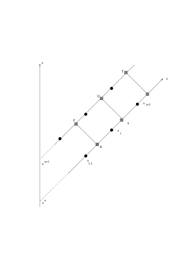
FIG. 1.: Line segments drawn at forty-five degrees represent radial characteristics. Their intersection defines the fundamental null parallelogram PQRS shown superimposed upon the computational cell, which consists of the points marked by circles and their nearest neighbors in the angular direction.

FIG. 2.: The error, as measured by the $L_{2}$ norm, of a numerical solution with higher harmonics ($\ell=6$). The computation is made on grids of size $N_{x}$ equal to 24, 48, 72, 96 and 120, while keeping $N_{x}=3N_{y}$.

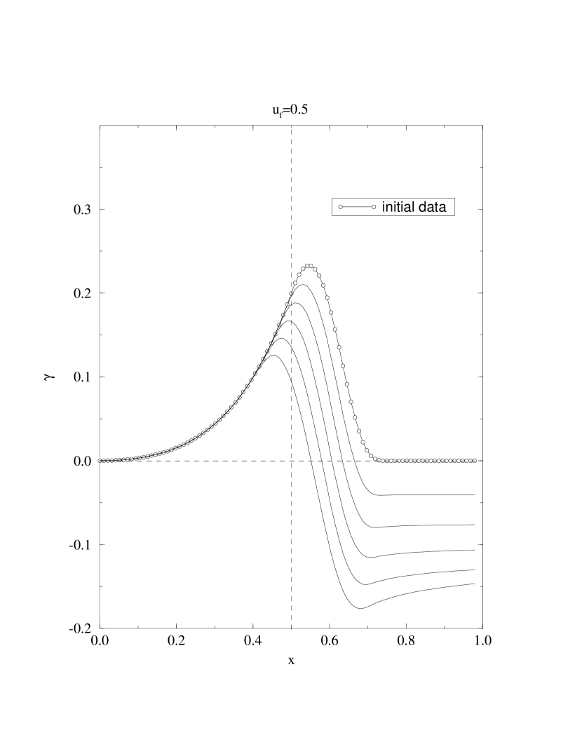
FIG. 3.: Evolution of initial data given by SIMPLE in the interior region, and patched smoothly to an asymptotically flat exterior. The static interior is preserved to graphical accuracy.

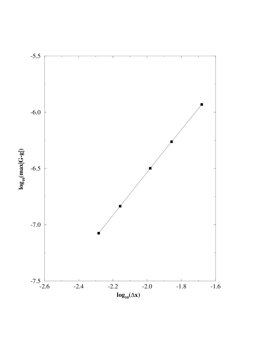
FIG. 4.: The error in the evolution of the initial data of Fig. 3 up to $u=0.25$, as measured by the $L_{\infty}$ norm. The error is computed on grids of size $N_{y}$ equal to 16, 24, 32, 48 and 64, while keeping $N_{x}=3N_{y}$. The convergence rate is $1.92$, in good agreement with the theoretically expectation of second order accuracy.

FIG. 5.: A sequence of time slices of the numerical evolution of initial data of compact support. Note all the angular structure that arises at about $u=0.25$, which later decays. At $u\approx 1.5$ the amplitude of the field has decayed below those values which can be observed in the figure.

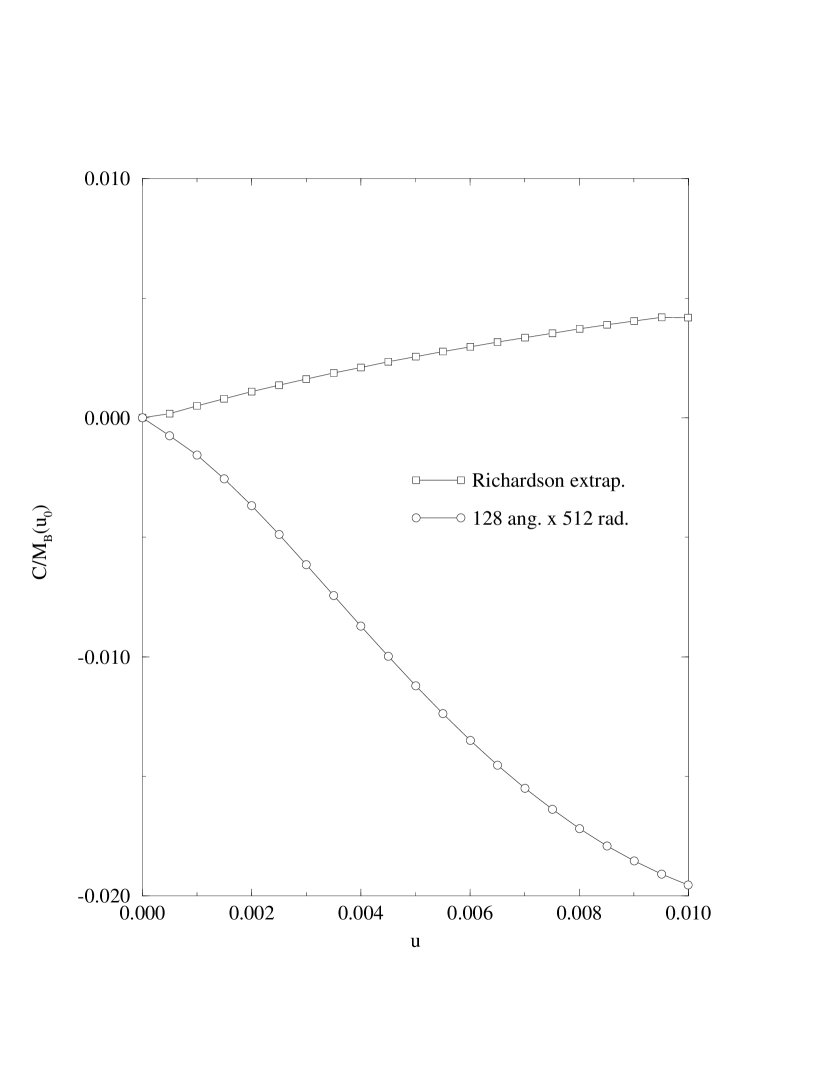
FIG. 6.: Graph of the relative error in $C$ calculated up to $u=0.01$ for a numerical evolution of the data (91), on a grid of 512 radial $\times$ 128 angular points. The circles show the error as calculated from the computed values of the mass, while the squares show the error after using Richardson extrapolation, based on the known convergence rate of the algorithm.

REFERENCES

- [1] R. Isaacson, J. Welling, and J. Winicour, J. Math. Phys. 24, 1824 (1983).
- [2] R. Gómez and J. Winicour, J. Math. Phys. 33, 1445 (1992).
- [3] R. Gómez and J. Winicour, Phys. Rev. D 45, 2776 (1992).
- [4] R. Gómez and J. Winicour, in Approaches to Numerical Relativity, edited by R. d’Inverno (Cambridge University Press, Cambridge, 1992).
- [5] R. Gómez, R. Isaacson, and J. Winicour, J. Comp. Phys. 98, 11 (1992).
- [6] M. van der Burg, H. Bondi, and A. Metzner, Proc. R. Soc. London Ser. A 269, 21 (1962).
- [7] R. Penrose and W. Rindler, Spinors and Space-Time, Vol. 1 (Cambridge University Press, Cambridge, 1984).
- [8] E. Newman and R. Penrose, Proc. R. Soc. London Ser. A 305, 175 (1968).
- [9] R. d’Inverno and J. Smallwood, Phys. Rev. D 22, 1223 (1980).
- [10] J. Bic̆ák and B. G. Schmidt, Phys. Rev. D 40, 1827 (1989).
- [11] J. Bic̆ák, P. Reilly, and J. Winicour, Gen. Rel. Grav. 20, 171 (1988).
- [12] R. Gómez, P. Reilly, J. Winicour, and R. A. Isaacson, Phys. Rev. D 47, 3292 (1993).
- [13] D. Christodoulou and S. Klainerman, The Global Nonlinear Stability of the Minkowski Space (Princeton University Press, Princeton, 1993).