Abstract

We rigorously analyze the frequency response functions and antenna sensitivity patterns of three types of interferometric detectors to scalar mode of gravitational waves which is predicted to exist in the scalar-tensor theory of gravity. By a straightforward treatment, we show that the antenna sensitivity pattern of the simple Michelson interferometric detector depends strongly on the wave length $\lambda_{\rm SGW}$ of the scalar mode of gravitational waves if $\lambda_{\rm SGW}$ is comparable to the arm length of the interferometric detector. For the Delay-Line and Fabry-Perot interferometric detectors with arm length much shorter than $\lambda_{\rm SGW}$, however, the antenna sensitivity patterns depend weakly on $\lambda_{\rm SGW}$ even though $\lambda_{\rm SGW}$ is comparable to the effective path length of those interferometers. This agrees with the result obtained by Maggiore and Nicolis.

PACS numbers: 04.30.Nk, 04.80.Nn, 04.50.+h

I Introduction

To detect gravitational waves in the frequency band between $\sim 100$ and $\sim 1000$Hz, the TAMA300 has been constructed [1] and TAMA300 team has already carried out several data taking runs [2]. Other kilometer-size interferometric detectors such as LIGO, VIRGO and GEO600 are also now under construction and will be in operation within a couple of years [3, 4, 5]. In addition, the Laser Interferometer Space Antenna (LISA) is now planned to be constructed in the next decade [6] to detect gravitational waves in the frequency band between $\sim 10^{-4}$ and $\sim 0.1$Hz. Main purposes of these projects are (i) the detection of gravitational waves and (ii) the observation of relativistic astrophysical phenomena in a strong gravitational field. The purpose (i) is related to a fundamental question on the correctness of general relativity because the detection of gravitational waves could give a strong constraint about number of modes and propagation speed of gravitational waves [7].

As an alternative candidate of general relativity, the scalar-tensor theory of gravity [8, 9] has recently received a renewed interest. One of the reasons for its revival is that a theoretical approach to unification of interactions in terms of superstring theories suggests that the theory of gravity should be the dilatonic one (a kind of the scalar-tensor theory) rather than general relativity, i.e., the pure tensor theory [10].

In [11], Shibata, Nakao and Nakamura investigated the gravitational collapse of a spherically symmetric dust ball to be a black hole in the framework of the Brans-Dicke theory (see also [12] and [13]). They found that the amplitude of scalar gravitational waves can be

$$\sim 10^{-21}\biggl{(}{M\over 10M_{\odot}}\biggr{)}\biggl{(}{3{\rm kpc}\over r}\biggr{)}\biggl{(}{5000\over\omega}\biggr{)},$$ (1)

or equivalently

$$\sim 10^{-21}\biggl{(}{M\over 10^{6}M_{\odot}}\biggr{)}\biggl{(}{3000{\rm Mpc}\over r}\biggr{)}\biggl{(}{5000\over\omega}\biggr{)},$$ (2)

with the frequency $\sim 100(10M_{\odot}/M)=10^{-3}(10^{6}M_{\odot}/M)$Hz which is in an appropriate frequency range for kilometer-size detectors and LISA, respectively. Here, $M$, $M_{\odot}$, $r$, and $\omega$ are the mass of the collapsed object, solar mass, distance from the source to the detectors, and the so-called Brans-Dicke parameter, respectively. The noise level of the advanced kilometer-size detectors and LISA will be $\sim 10^{-23}$ for the most sensitive frequency band. Thus, although the present experimental limit is stringent $\omega>3300$ [14], the amplitude of scalar gravitational waves may be high enough to be detected by the interferometric detectors if stellar mass black holes are formed in our galaxy or if supermassive black holes are formed in the cosmological scale.

As pointed out in [11] and reanalyzed by Maggiore and Nicolis [15], the antenna sensitivity pattern of interferometric detectors to the scalar mode is different form that of the tensor mode. This implies that if four interferometric detectors which are coincidently in operation detects gravitational waves, it is possible to ask whether the scalar mode exists or not using the difference of the arrival time and the difference of the antenna pattern among four detectors [16]. Also, the peak frequency of the scalar mode is likely different from that of the tensor mode [17, 18], suggesting that the two modes could be distinguished in the frequency domain even in the case of one interferometer. Thus, for exploration of the correctness of general relativity using interferometric detectors, it is important to clarify the antenna sensitivity pattern and frequency response function not only for the tensor mode but for the scalar mode of gravitational waves. From this motivation, analyses have been carried out in [11][15] so far, but they were too crude [11] or approximate [15]. In this article, we carry out a rigorous reanalysis of the frequency response function and antenna sensitivity pattern of the interferometric detector to the scalar mode without any approximation: We directly solve the Maxwell equation for the propagation of a laser ray and the geodesic equation for motion of mirrors and a beam splitter in contrast to a previous work [15]. Our straightforward treatment enables us to investigate the dependence of the antenna sensitivity pattern on the wave length of the scalar mode of gravitational waves without any ambiguity.

This article is organized as follows. In Sec. II, we briefly review the linearized equation for gravitational waves in the framework of the scalar-tensor theory of gravity. In Sec. III, we solve the Maxwell field equation in the spacetime with the scalar mode of gravitational waves to derive a plane wave solution which describes the path of a laser ray in the interferometric detector. In Sec. IV, we present explicit solutions for timelike geodesics in the presence of scalar gravitational waves, since the mirrors and beam splitter in the interferometric detector move along timelike geodesics. We present the dependence of the frequency response function and antenna sensitivity pattern of Michelson interferometric detectors on the frequency of the scalar mode of gravitational waves in Sec. V, and of Delay-Line (DL) and Fabry-Perot (FP) interferometric detectors in Sec. VI. Sec. VII is devoted to a summary.

We adopt the unit in which the speed of light is unity. We follow the convention of the metric and Riemann tensor in [19]. Throughout this article, we adopt the abstract index notation; The Latin indices $a,...,d$ denote a type of tensor, Greek indices components of a tensor, and two Latin indices, $i$ and $j$, the spatial components of a tensor.

II Gravitational Waves in the Scalar-Tensor Theory

The field equation for the tensor part in the scalar-tensor theory of gravity is written in the form [8, 9]

$$G_{ab}={8\pi\over\Phi}T_{ab}+{\omega(\Phi)\over\Phi^{2}}\Bigl{[}(\nabla_{a}\Phi)\nabla_{b}\Phi-{1\over 2}g_{ab}(\nabla^{c}\Phi)\nabla_{c}\Phi\Bigr{]}+{1\over\Phi}(\nabla_{a}\nabla_{b}\Phi-g_{ab}\nabla^{c}\nabla_{c}\Phi),$$ (3)

where $G_{ab}$ and $\nabla_{a}$ are the Einstein tensor and covariant derivative with respect to $g_{ab}$, respectively. The function, $\omega(\Phi)$, is the coupling function which determines the coupling strength between the gravitational scalar field, $\Phi$, and the spacetime geometry. $T_{ab}$ is the energy-momentum tensor of matter or radiation. The field equations for the scalar field $\Phi$ and matter are given by

$$\nabla^{c}\nabla_{c}\Phi={1\over 2\omega+3}\Bigl{[}8\pi T^{c}_{c}-{d\omega\over d\Phi}(\nabla^{c}\Phi)\nabla_{c}\Phi\Bigr{]},$$ (4)

and

$$\nabla_{a}T^{ab}=0.$$ (5)

In the Brans-Dicke theory, $\omega$ is a finite constant and in general relativity, $\omega=\infty$. Note that measurement of a gravitational lensing angle of a light ray from a distant quasar by the gravity of the Sun now constrains $|\omega|$ to be $>3300$ [14].

Since the interferometric detectors are located in the wave zone of gravitational waves, we need to consider the linearized, vacuum $(T_{ab}=0)$ field equations. We write the metric tensor and gravitational scalar field in the forms

$$g_{ab} = \eta_{ab}+h_{ab},$$ (6)

$$\Phi = \Phi_{0}(1-\delta\Phi),$$ (7)

where $\eta_{ab}$ is the metric tensor of the background Minkowski spacetime and $\Phi_{0}$ is the value of $\Phi$ in the infinity. We assume that magnitude of each component of the perturbations $h_{ab}$ and $\delta\Phi$ is much smaller than unity. The linearized equations for the metric tensor and gravitational scalar field are written as

$$-{1\over 2}\partial^{c}\partial_{c}{\bar{h}}_{ab}-{1\over 2}\eta_{ab}\partial_{c}\partial_{d}{\bar{h}}^{cd}+\partial_{c}\partial_{(a}{\bar{h}}^{c}_{b)}=-\partial_{a}\partial_{b}\delta\Phi+\eta_{ab}\partial^{c}\partial_{c}\delta\Phi,$$ (8)

and

$$\partial^{c}\partial_{c}\delta\Phi=0,$$ (9)

where

$$h^{a}_{b} \equiv \eta^{ac}h_{cb},$$ (10)

$${\bar{h}}_{ab} \equiv h_{ab}-{1\over 2}\eta_{ab}h^{c}_{c},$$ (11)

$$\partial^{c} \equiv \eta^{cd}\partial_{d}.$$ (12)

Introducing a new symmetric tensor field ${\tilde{h}}_{ab}$ defined by

$${\tilde{h}}_{ab}\equiv{\bar{h}}_{ab}+\eta_{ab}\delta\Phi,$$ (13)

Eq. (8) is rewritten to

$$-{1\over 2}\partial^{c}\partial_{c}{\tilde{h}}_{ab}-{1\over 2}\eta_{ab}\partial_{c}\partial_{d}{\tilde{h}}^{cd}+\partial_{c}\partial_{(a}{\tilde{h}}^{c}_{b)}=0.$$ (14)

Equation (14) is completely the same as the linearized Einstein equation for the trace-reversed metric perturbations [19]. This enables us to impose the transverse-traceless gauge condition on ${\tilde{h}}_{ab}$ as in general relativity as

$$\partial_{a}{\tilde{h}}_{b}^{a} = 0,$$ (15)

$${\tilde{h}}_{a0} = 0.$$ (16)

Under this gauge condition, the line element in the wave zone is written in the following form,

$$ds^{2}=(1+\delta\Phi)\left\{-dt^{2}+(\delta_{ij}+{h}_{ij}^{\rm TT})d{\bar{x}}^{i}d{\bar{x}}^{j}\right\},$$ (17)

where $h_{ij}^{\rm TT}\equiv{\tilde{h}}_{ij}$ is the transverse-traceless spatial tensor which satisfies

$$\partial^{c}\partial_{c}h^{\rm TT}_{ij}=0.$$ (18)

From Eq. (17), $h^{\rm TT}_{ij}$ and $\delta\Phi$ are regarded as the tensor and scalar modes of gravitational waves, respectively, which constitute three independent modes of gravitational waves in the scalar-tensor theory. Hereafter, we refer to the scalar mode as scalar gravitational waves (SGW).

In the rest of this article, we assume that the amplitude of the tensor mode $h^{\rm TT}_{ij}$ is much smaller than that of SGW for simplicity. Such a situation is realized when the source of the gravitational radiation is almost spherically symmetric. We also assume

$$\delta\Phi=\delta\Phi(t+{\bar{z}}),$$ (19)

in the coordinate system (17).

III Maxwell Field

A trajectory of a laser ray is determined by solving the source-free Maxwell equation as

$$g^{ac}\nabla_{a}F_{cb}=0,$$ (20)

where

$$F_{ab}\equiv\nabla_{a}A_{b}-\nabla_{b}A_{a}=\partial_{a}A_{b}-\partial_{b}A_{a}.$$ (21)

From Eq. (17), we find that the line element takes conformally flat form in the coordinate system adopted here and in the absence of the tensor modes. Then, Eq. (20) is rewritten to

$$g^{ac}\nabla_{a}F_{cb}=(1+\delta\Phi)^{-2}\eta^{ac}\partial_{a}F_{cb}=(1+\delta\Phi)^{-2}(\partial^{a}\partial_{a}A_{b}-\partial^{a}\partial_{b}A_{a})=0.$$ (22)

Adopting the Lorentz gauge condition $\partial^{a}A_{a}=0$, we obtain the equation for the vector potential $A_{a}$ as

$$\partial^{a}\partial_{a}A_{b}=0.$$ (23)

Note that Eq. (23) is of the same form as the equation in the Minkowski spacetime.

In the geometrical approximation, a laser ray is regarded as a monochromatic plane wave in the absence of SGW, i.e.,

$$A_{\mu}={\cal A}_{\mu}\exp\left\{i\Omega_{\rm L}(t-{\vec{c}}_{\rm L}\cdot{\vec{r}})\right\},$$ (24)

where ${\cal A}_{\mu}$, $\Omega_{\rm L}$, ${\vec{c}}_{\rm L}$ and ${\vec{r}}$ are the constant amplitude, constant angular frequency of the laser ray for the rest observer, constant direction cosine of the laser ray and position vector in the conformal 3D space, respectively. Eq. (23) implies that even in the presence of SGW, the components of the vector potential $A_{\mu}$ is completely the same as in Eq. (24), and the trajectory of the laser ray is straight in the conformal 3D space, i.e.,

$${d{\vec{r}}\over dt}={\vec{c}}_{\rm L}.$$ (25)

From the above result, one might think that the laser interferometric detector could not detect SGW since SGW do not affect the Maxwell field described in the conformally flat coordinate system. However this is the misunderstanding. We should take into account that the laser ray is repeatedly reflected by mirrors which are perturbed in the presence of SGW. This non-trivial perturbed motion causes variations of the vector potential $A_{\mu}$ and consequently generates side-band waves which are just observed by interferometric detectors.

IV Timelike Geodesics

The mirrors and beam splitter are suspended by wires so that they can freely move at frequencies much higher than the pendulum frequencies. For simplicity, we assume that the emitter of laser rays is also a free mass. Then, the trajectories of these parts of detectors are determined by solving the timelike geodesics in the spacetime described by (17).

Introducing the retarded and advanced time coordinates $u$ and $v$,

$$u=t-{\bar{z}}~{}~{}~{}~{}~{}{\rm and}~{}~{}~{}~{}~{}v=t+{\bar{z}},$$ (26)

equations for a timelike geodesic are given by

$${d\over d\tau}\left\{(1+\delta\Phi){d{\bar{x}}\over d\tau}\right\} = 0,$$ (27)

$${d\over d\tau}\left\{(1+\delta\Phi){d{\bar{y}}\over d\tau}\right\} = 0,$$ (28)

$${d\over d\tau}\left\{(1+\delta\Phi){dv\over d\tau}\right\} = 0,$$ (29)

and

$${d\over d\tau}\left\{(1+\delta\Phi){dv\over d\tau}\right\}=-{d\delta\Phi\over dv}.$$ (30)

Hereafter, we assume that the mirrors and beam splitter are at rest in the absence of SGW. In this case, we can set $\delta\Phi=0$ using freedom to scale the coordinates. Integrating Eqs. (27)$-$(30), we obtain

$${d{\bar{x}}\over d\tau}={d{\bar{y}}\over d\tau}=0,$$ (31)

and

$${dv\over d\tau}=C_{v}(1-\delta\Phi),$$ (32)

where $C_{v}$ is an integration constant. From the normalization of the geodesic tangent vector and the above equation, we derive

$${du\over d\tau}={1\over C_{v}}.$$ (33)

Since $d{\bar{z}}/d\tau=0$ and $dt/d\tau=1$ for $\delta\Phi=0$, the integration constant $C_{v}$ is equal to 1. As a result, we find

$${dt\over d\tau} = 1-{1\over 2}\delta\Phi(v),$$ (34)

$${d{\bar{z}}\over d\tau} = -{1\over 2}\delta\Phi(v).$$ (35)

By integrating Eqs. (31)–(35), the trajectory of a free mass is derived as

$${\bar{x}} = {\bar{x}}_{\rm i},$$ (36)

$${\bar{y}} = {\bar{y}}_{\rm i},$$ (37)

$${\bar{z}} = -{1\over 2}\int^{\tau}\delta\Phi(v)d\tau={\bar{z}}_{\rm i}-{1\over 2}\int_{-\infty}^{t+{\bar{z}}_{\rm i}}\delta\Phi(v)dv,$$ (38)

where ${\bar{x}}_{\rm i}$, ${\bar{y}}_{\rm i}$ and ${\bar{z}}_{\rm i}$ are integration constants which specify the location of the free mass in this coordinate system (17) for $t\rightarrow-\infty$, and we have used

$${d\tau\over dv}=1+\delta\Phi.$$ (39)

Then, we derive a trajectory of a free mass for an arbitrary incoming direction of SGW, which is obtained by a spatial rotation of the coordinate system (17) as

$$\left(\begin{array}[]{c}x\\ y\\ z\\ \end{array}\right)=\left(\begin{array}[]{ccc}\cos\theta\cos\varphi&-\sin\varphi&\sin\theta\cos\varphi\\ \cos\theta\sin\varphi&\cos\varphi&\sin\theta\sin\varphi\\ -\sin\theta&0&\cos\theta\\ \end{array}\right)\left(\begin{array}[]{c}{\bar{x}}\\ {\bar{y}}\\ {\bar{z}}\\ \end{array}\right)~{}~{},$$ (40)

where the direction cosine ${\vec{c}}_{\rm SGW}$ of SGW in the new coordinate system is

$${\vec{c}}_{\rm SGW}=(-\sin\theta\cos\varphi,-\sin\theta\sin\varphi,-\cos\theta).$$ (41)

The explicit form of the trajectory of the free mass in the new coordinate system is written as

$$x = x_{\rm i}-{1\over 2}\sin\theta\cos\varphi\int_{-\infty}^{t+\Lambda}\delta\Phi(v)dv,$$ (42)

$$y = y_{\rm i}-{1\over 2}\sin\theta\sin\varphi\int_{-\infty}^{t+\Lambda}\delta\Phi(v)dv,$$ (43)

$$z = z_{\rm i}-{1\over 2}\cos\theta\int_{-\infty}^{t+\Lambda}\delta\Phi(v)dv,$$ (44)

where $x_{\rm i}$, $y_{\rm i}$ and $z_{\rm i}$ are constants which specify the location of the free mass in this new coordinate system in the infinite past $t\rightarrow-\infty$, and

$$\Lambda\equiv x_{\rm i}\sin\theta\cos\varphi+y_{\rm i}\sin\theta\sin\varphi+z_{\rm i}\cos\theta.$$ (45)

Since the spacetime metric takes conformally flat form in the absence of the tensor modes, we might think that SGW would be longitudinal wave. However, from careful investigation of the geodesic deviation equation, we find that the tidal force associated with SGW acts along the directions orthogonal to the propagation direction of SGW [9]. From this point of view, SGW should be regarded as the transverse wave. It is also worthy to note that even if free masses are at rest in the present coordinate, the relative distances between them are not necessarily constant if SGW exist. Converse is also true.

V Detection of SGW by a Simple Michelson Interferometer

In the following, we identify the $x$ and $y$ axes with the directions of arms of the interferometric detector (cf, Fig. 1). We hereafter refer to the arm on the $x$ ($y$) axis as Arm1 (Arm2).

In the Michelson interferometric detectors, a laser ray first reaches the beam splitter and then is divided into two rays; one enters into the Arm1 and the other into the Arm2. Each ray is reflected by the mirrors and then returns to the beam splitter again. The path difference of the two arms is chosen in such a way that the interfering light is dark at the anti-symmetric port for achieving the best signal-to-noise ratio. Here, we focus on two rays which finally reach $x=0$ on the beam splitter coincidently at $t=t_{\rm B}$ (cf, Fig. 1).

To calculate the side-band waves of laser rays, we need the trajectories of the beam splitter and mirrors only in the $x$-$y$ plane. Using Eqs. (42)–(44), we obtain the trajectory of the center of the beam splitter as

$$x = x_{\rm B}(t)=-{1\over 2}\sin\theta\cos\varphi\int_{-\infty}^{t}\delta\Phi(v)dv,$$ (46)

$$y = y_{\rm B}(t)=-{1\over 2}\sin\theta\sin\varphi\int_{-\infty}^{t}\delta\Phi(v)dv.$$ (47)

The trajectory of the mirror in Arm1 is given by

$$x=x_{\rm M}(t)=L_{1}-{1\over 2}\sin\theta\cos\varphi\int_{-\infty}^{t+X}\delta\Phi(v)dv,$$ (48)

where

$$X=L_{1}\sin\theta\cos\varphi.$$ (49)

Note that we do not need the $y$-coordinate of this mirror for calculating the side-band waves since the motion in the $y$-direction does not affect the path difference in the linear order in $\delta\Phi$. From essentially the same procedure, the trajectory of the mirror in Arm2 is given by

$$y=y_{\rm M}(t)=L_{2}-{1\over 2}\sin\theta\sin\varphi\int_{-\infty}^{t+Y}\delta\Phi(v)dv,$$ (50)

where

$$Y=L_{2}\sin\theta\sin\varphi.$$ (51)

In this case, it is not necessary to know the $x$-coordinate of this mirror.

The trajectory of the emitter is written as

$$x=x_{\rm E}(t)=-\ell_{\rm E}-{1\over 2}\sin\theta\cos\varphi\int_{-\infty}^{t+X_{\rm E}}\delta\Phi(v)dv,$$ (52)

where

$$X_{\rm E}=-\ell_{\rm E}\sin\theta\cos\varphi.$$ (53)

Information of the $y$-coordinate of the emitter is also not necessary.

Since we regard the emitter as a free mass, we need to carefully treat the phase of the laser ray. The amplitude $A$ of the laser ray at the emitter is written as

$$A={\cal A}_{\rm L}e^{i\Omega_{\rm L}\tau_{\rm E}},$$ (54)

where ${\cal A}_{\rm L}$ and $\Omega_{\rm L}$ are constant and $\tau_{\rm E}$ is the proper time of the emitter. The relation between the coordinate time $t$ and proper time $\tau_{\rm E}$ is given by Eq. (34). Integrating this equation, we obtain

$$\tau_{\rm E}(t)=t+{1\over 2}\int_{-\infty}^{t+X_{\rm E}}\delta\Phi(v)dv.$$ (55)

Thus, the amplitude $A$ is expressed as a function of $t$ as

$$A(t)={\cal A}_{\rm L}\exp\left\{i\Omega_{\rm L}\left(t+{1\over 2}\int_{-\infty}^{t+X_{\rm E}}\delta\Phi(v)dv\right)\right\}.$$ (56)

Then, we consider the ray entering into Arm1. Tracking from $t=t_{\rm B}$ toward the past, the laser ray reached the mirror in Arm1 at $t=t_{\rm B}-L_{1}+O(\delta\Phi)$, and then it reached the emitter at $t=t_{B}-2L_{1}-\ell_{\rm E}+O(\delta\Phi)$. As shown in Eq. (24), the plane wave solution of the Maxwell equation is completely the same as that of the Minkowski spacetime in the conformally flat coordinate system. This implies that the amplitude $A_{1}$ of the laser ray at the beam splitter agrees with the amplitude $A$ at the emitter at $t=t_{\rm B}-r_{1}$, where $r_{1}$ is the coordinate path length of this ray from the emitter to the final beam splitter. Using Eq. (56), we obtain the amplitude $A_{1}$ of the laser ray at the beam splitter on the output port side at $t=t_{\rm B}$ as

$$A_{1}=A(t_{\rm B}-r_{1})=\rho_{\rm B}\nu_{\rm B}{\cal A}_{\rm L}\exp\left\{i\Omega_{\rm L}\left(t_{B}-r_{1}+{1\over 2}\int_{-\infty}^{t_{\rm B}-r_{1}+X_{\rm E}}\delta\Phi(v)dv\right)\right\},$$ (57)

where $\rho_{\rm B}$ is a reflection coefficient from the detector side ($-\rho_{\rm B}$ from the laser side) and $\nu_{\rm B}$ is transmission coefficient of the beam splitter.

From the mirror at $t=t_{\rm B}-L_{1}+O(\delta\Phi)$ to the beam splitter at $t=t_{\rm B}$, the coordinate path length of the laser ray is equal to $x_{\rm M}(t_{\rm B}-L_{1})+O(\delta\Phi^{2})$, and from the beam splitter at $t=t_{\rm B}-2L_{1}+O(\delta\Phi)$ to the mirror at $t=t_{\rm B}-L_{1}+O(\delta\Phi)$, the coordinate path length is $x_{\rm M}(t_{\rm B}-L_{1})+O(\delta\Phi^{2})$. From the emitter at $t=t_{\rm B}-2L_{1}-\ell_{\rm E}+O(\delta\Phi)$ to the beam splitter at $t=t_{\rm B}-2L_{1}+O(\delta\Phi)$, the coordinate path length is $-x_{\rm E}(t_{\rm B}-2L_{1}-\ell_{\rm E})+O(\delta\Phi^{2})$. Thus, $r_{1}$ is given by

$$r_{1} = x_{\rm M}(t_{\rm B}-L_{1})+x_{\rm M}(t_{\rm B}-L_{1})-x_{\rm E}(t_{\rm B}-2L_{1}-\ell_{\rm E})$$ (58)

$$= 2L_{1}+\ell_{\rm E}+{1\over 2}\left(2\int_{-\infty}^{t_{\rm B}-L_{1}+X}-\int_{-\infty}^{t_{\rm B}-2L_{1}-\ell_{\rm E}+X_{\rm E}}\right)\delta\Phi(v)dv.$$ (59)

Substituting the above expression into Eq. (57), the amplitude $A_{1}$ is written in the form

$$A_{1}=\rho_{\rm B}\nu_{\rm B}{\cal A}_{\rm L}e^{i\Omega_{\rm L}(t_{\rm B}-2L_{1}-\ell_{\rm E})}\left\{1+\Delta A_{1}+O(\delta\Phi^{2})\right\},$$ (60)

where

$$\Delta A_{1} \equiv {i\over 2}\Omega_{\rm L}\Biggl{\{}\sin\theta\cos\varphi\left(2\int_{-\infty}^{t_{\rm B}-L_{1}+X}-\int_{-\infty}^{t_{\rm B}-2L_{1}-\ell_{\rm E}+X_{\rm E}}\right)+\int_{-\infty}^{t_{\rm B}-2L_{1}-\ell_{\rm E}+X_{\rm E}}\Biggr{\}}\delta\Phi(v)dv.$$ (61)

From the same procedure as that for the laser ray entering into Arm1, the amplitude $A_{2}$ at the beam splitter on the output port side for the laser ray entering into Arm2 is expressed in the form

$$A_{2}=A(t_{\rm B}-r_{2})=-\rho_{\rm B}\nu_{\rm B}{\cal A}_{\rm L}\exp\left\{i\Omega_{\rm L}\left(t_{B}-r_{2}+{1\over 2}\int_{-\infty}^{t_{\rm B}-2L_{2}-\ell_{\rm E}+X_{\rm E}}\delta\Phi(v)dv\right)\right\},$$ (62)

where $r_{2}$ is the coordinate path length of this ray from the emitter to the final beam splitter.

As shown in Fig. 1, the trajectory of the laser ray considered here is restricted on the straight line $x=0$ when it goes through the Arm2. Thus, this laser ray comes back to the beam splitter first at

$$y=y_{\rm B}(t_{\rm B}-2L_{2})-x_{\rm B}(t_{\rm B}-2L_{2}),$$ (63)

and finally at

$$y=y_{\rm B}(t_{\rm B})-x_{\rm B}(t_{\rm B}).$$ (64)

From the same procedure as in the case of Arm1, the coordinate path length $r_{2}$ from the emitter to the final beam splitter is given by

$$r_{2} = y_{\rm M}(t_{\rm B}-L_{2})-\left\{y_{\rm B}(t_{B})-x_{\rm B}(t_{B})\right\}$$ (65)

$$+ y_{\rm M}(t_{\rm B}-L_{2})-\left\{y_{\rm B}(t_{\rm B}-2L_{2})-x_{\rm B}(t_{\rm B}-2L_{2})\right\}$$ (66)

$$- x_{\rm E}(t_{\rm B}-2L_{2}-\ell_{\rm E})$$ (67)

$$= 2L_{2}+\ell_{\rm E}-{1\over 2}\sin\theta\Biggl{\{}\cos\varphi\left(\int_{-\infty}^{t_{\rm B}}+\int_{-\infty}^{t_{\rm B}-2L_{2}}-\int_{-\infty}^{t_{\rm B}-2L_{2}-\ell_{\rm E}+X_{\rm E}}\right)$$ (68)

$$+ \sin\varphi\left(\int_{t_{\rm B}}^{t_{\rm B}-L_{2}+Y}+\int_{t_{\rm B}-2L_{2}}^{t_{\rm B}-L_{2}+Y}\right)\Biggr{\}}\delta\Phi(v)dv.$$ (69)

Substituting the above equation into Eq. (62), we obtain

$$A_{2}=-\rho_{\rm B}\nu_{\rm B}A_{\rm L}e^{i\Omega_{\rm L}(t_{\rm B}-2L_{2}-\ell_{\rm E})}\left\{1+\Delta A_{2}+O(\delta\Phi^{2})\right\},$$ (70)

at the final beam splitter, where

$$\Delta A_{2} \equiv {i\over 2}\Omega_{\rm L}\Biggl{\{}\sin\theta\cos\varphi\left(\int_{-\infty}^{t_{\rm B}}+\int_{-\infty}^{t_{\rm B}-2L_{2}}-\int_{-\infty}^{t_{\rm B}-2L_{2}-\ell_{\rm E}+X_{\rm E}}\right)$$ (71)

$$+ \sin\theta\sin\varphi\left(\int_{t_{\rm B}}^{t_{\rm B}-L_{2}+Y}+\int_{t_{\rm B}-2L_{2}}^{t_{\rm B}-L_{2}+Y}\right)+\int_{-\infty}^{t_{\rm B}-L_{2}-\ell_{\rm E}+X_{\rm E}}\Biggr{\}}\delta\Phi(v)dv.$$ (72)

To maintain the output port to be dark in the absence of SGW $\delta\Phi=0$, the following condition should be satisfied

$$\Omega_{\rm L}(L_{1}-L_{2})=m\pi,$$ (73)

where $m$ is integer. Therefore, in the presence of SGW, the side-band waves are generated with the amplitude

$$A_{\rm out} = A_{1}+A_{2}$$ (74)

$$= \rho_{\rm B}\nu_{\rm B}A_{\rm L}e^{i\Omega_{\rm L}(t_{\rm B}-2L_{1}-\ell_{\rm E})}(\Delta A_{1}-\Delta A_{2})$$ (75)

$$= \rho_{\rm B}\nu_{\rm B}A_{\rm L}\Omega_{\rm L}e^{i\Omega_{\rm L}(t_{\rm B}-2L_{1}-\ell_{\rm E})}\int_{-\infty}^{+\infty}\delta{\tilde{\Phi}}(\omega)e^{i\omega t_{\rm B}}H_{\rm M}(\omega)d\omega,$$ (76)

where

$$\delta{\tilde{\Phi}}(\omega)\equiv{1\over 2\pi}\int_{-\infty}^{+\infty}e^{-i\omega v}\delta\Phi(v)dv,$$ (77)

and $H_{\rm M}(\omega)$ is a frequency response function to SGW of Michelson interferometric detectors. (Note that hereafter $\omega$ does not denote the Brans-Dicke parameter but the angular frequency.) It is worthy to note that difference between the coordinate time $t_{\rm B}$ and the proper time at the detector is $O(\delta\Phi)$ so that it only contributes to a higher order correction for the side-band waves.

The explicit form of $H_{\rm M}(\omega)$ is

$$H_{\rm M}(\omega) = {1\over 2\omega}\sin\theta\Biggl{\{}\cos\varphi\left(2e^{i\omega L_{1}(\sin\theta\cos\varphi-1)}-1-e^{-2i\omega L_{1}}\right)$$ (78)

$$- \sin\varphi\left(2e^{i\omega L_{2}(\sin\theta\sin\varphi-1)}-1-e^{-2i\omega L_{2}}\right)\Biggr{\}}.$$ (79)

For simplicity, we restrict our attention to the case

$$L_{1}=L_{2}=L.$$ (80)

Then, in the limit $\omega\rightarrow 0$, the response function becomes

$$\lim_{\omega\rightarrow 0}H_{\rm M}(\omega)=iL\sin^{2}\theta\cos 2\varphi,$$ (81)

which agrees with the antenna sensitivity pattern obtained by Maggiore and Nicolis [15]. However, for SGW of general frequency $\omega$, the antenna sensitivity pattern is different from Eq. (81) (cf, Fig. 2).

To see the dependence of the amplitude of $H_{\rm M}(\omega)$ on the frequency $\omega$ of SGW, we pay particular attention to the incident direction $\theta=\pi/2$ and $\varphi=0$. Then, we obtain

$$|H_{\rm M}(\omega)|^{2}={\sin^{2}(\omega L)\over\omega^{2}}.$$ (82)

Thus, Michelson interferometric detectors are sensitive to SGW of $\omega\lesssim\omega_{\rm M}$ where

$$\omega_{\rm M}\equiv\pi/(2L).$$ (83)

From Eq. (81), we find that the longer the arm length $L$ is, the better the sensitivity of Michelson detectors is. However, longer arm length leads to smaller upper bound $\omega_{\rm M}$ of the sensitive frequency range. To optimize the laser interferometric detector against SGW of an aimed frequency, the arm length of the laser ray should be equal to a quarter of the wave length of SGW.

The sensitivity patterns on $\theta=\pi/2$ plane for the frequency $\omega=\omega_{\rm M}$ of aimed SGW are shown in Fig. 2(a). Obviously, the sensitivity patterns for $\omega=\omega_{\rm M}$ and $\omega=\omega_{\rm M}/2$ are different from Eq. (81). On the other hand, for $\omega=\omega_{\rm M}/100$, i.e., when the wave length of SGW is $400L$, the sensitivity pattern is almost the same as that in Eq. (81). These consequences imply that the sensitivity pattern of Michelson interferometric detectors depends strongly on the frequency in the neighborhood of $\omega=\omega_{\rm M}$.

VI Detection of SGW by Delay-Line and Fabry-Perot Interferometers

As explained in the previous section, the arm length of Michelson interferometric detectors should be equal to a quarter of the wave length of SGW to optimize the sensitivity. The wave length of SGW generated by a spherical gravitational collapse to a black hole, however, could be $\sim 100(M/M_{\odot})$km for stellar mass black holes [11]. It is in practice difficult to construct a laser interferometric detector of such long arm length on the ground. Due to this reason, DL or FP interferometric detectors in which it is possible to make the effective optical path length much longer than the arm length have been adopted as ground-based detectors in practical projects. In this section, we study the frequency response function and antenna sensitivity pattern of DL and FP laser interferometric detectors.

Following the notation in Sec. V, we identify the $x$ and $y$ axes with the direction of the arms of the interferometric detector (cf, Fig. 3). We again refer to the arm on the $x$ ($y$) axis as Arm1 (Arm2). As in the case of Michelson detectors, we need the trajectories of the mirrors and beam splitter only in the $x$-$y$ plane. The trajectory of the center of the beam splitter is given by Eqs. (46) and (47). The trajectories of the front mirror and of the end mirror in Arm1 are given by

$$x=x_{\rm Mf}(t)=\ell_{1}-{1\over 2}\sin\theta\cos\varphi\int_{-\infty}^{t+X_{\rm f}}\delta\Phi(v)dv,$$ (84)

$$x=x_{\rm Me}(t)=L_{1}+\ell_{1}-{1\over 2}\sin\theta\cos\varphi\int_{-\infty}^{t+X_{\rm e}}\delta\Phi(v)dv,$$ (85)

where

$$X_{\rm f} = \ell_{1}\sin\theta\cos\varphi,$$ (86)

$$X_{\rm e} = (L_{1}+\ell_{1})\sin\theta\cos\varphi.$$ (87)

The trajectories of the front mirror and the end mirror in Arm2 are given by

$$y=y_{\rm Mf}(t)=\ell_{2}-{1\over 2}\sin\theta\sin\varphi\int_{-\infty}^{t+Y_{\rm f}}\delta\Phi(v)dv,$$ (88)

$$y=y_{\rm Me}(t)=L_{2}+\ell_{2}-{1\over 2}\sin\theta\sin\varphi\int_{-\infty}^{t+Y_{\rm e}}\delta\Phi(v)dv,$$ (89)

where

$$Y_{\rm f} = \ell_{2}\sin\theta\sin\varphi,$$ (90)

$$Y_{\rm e} = (L_{2}+\ell_{2})\sin\theta\sin\varphi.$$ (91)

We do not need to calculate the $y$-coordinates of mirrors in Arm 1 and the $x$-coordinates of mirrors in Arm2 to obtain side-band waves since the motion of these mirrors in these directions affects the path difference from the second order in $\delta\Phi$. The trajectory of the emitter and the amplitude $A$ of the laser ray at the emitter are given by Eq. (52) and by Eq. (56), respectively, as in Michelson detectors. However, the definitions of $L_{1}$ and $L_{2}$ are different from those in Michelson detectors (cf, Fig. 3).

A Delay-Line Interferometer

As in Michelson interferometric detectors, a laser ray in DL detectors first reaches the beam splitter and then is divided into two rays; one enters into the Arm1 and the other into the Arm2. In the DL detectors, however, the ray entering into the regions between the front and end mirrors is reflected by these mirrors by ($2N-1$) times until returning to the beam splitter again to increase an optical path length by $2N$ times as long as the arm length. This mechanism changes the response of the detector.

As in Sec. IV, we pay attention to two rays which finally reach the beam splitter coincidently at $t=t_{\rm B}$ (cf, Fig. 3). First, we consider the ray entering into Arm1. For notational convenience, we introduce

$$t_{{\rm f}(n)} = t_{\rm B}-\left\{\ell_{1}+(2n-2)L_{1}\right\},$$ (92)

$$t_{{\rm e}(n)} = t_{\rm B}-\left\{\ell_{1}+(2n-1)L_{1}\right\},$$ (93)

$$t_{{\rm E}(n)} = t_{\rm B}-\left(2\ell_{1}+\ell_{\rm E}+2nL_{1}\right).$$ (94)

From the same procedure as in Michelson interferometric detectors, the amplitude $A_{1}$ of the $N$-fold ray at the beam splitter on the output port side is expressed in the form

$$A_{1}=\rho_{\rm B}\nu_{\rm B}A_{\rm L}\exp\left\{i\Omega_{\rm L}\left(t_{B}-r_{(N)}+{1\over 2}\int_{-\infty}^{t_{{\rm E}(N)}+X_{\rm E}}\delta\Phi(v)dv\right)\right\},$$ (95)

where the definition of $\rho_{\rm B}$ and $\nu_{\rm B}$ are the same as for the Michelson detector, and $r_{(N)}$ is the coordinate path length of this ray from the emitter to the final beam splitter.

In the following calculation for the coordinate path length $r_{(N)}$, we assume that the trajectory of the ray is parallel to the $x$-axis. Strictly speaking, the ray is not parallel to the $x$-axis in a real DL interferometric detector, but the effect of it on the path length is the second order in $\delta\Phi$. Then we obtain

$$r_{(N)} = x_{{\rm Mf}}(t_{{\rm f}(1)})+\sum_{k=1}^{N}\left\{2x_{{\rm Me}}(t_{{\rm e}(k)})-x_{{\rm Mf}}(t_{{\rm f}(k)})-x_{{\rm Mf}}(t_{{\rm f}(k+1)})\right\}+x_{{\rm Mf}}(t_{{\rm f}(N+1)})-x_{{\rm E}}(t_{{\rm E}(N)})$$ (96)

$$= 2\ell_{1}+\ell_{\rm E}+2NL_{1}+\Delta R_{(N)},$$ (97)

where

$$\Delta R_{(N)} = -{1\over 2}\sin\theta\cos\varphi\Biggl{\{}\int_{-\infty}^{t_{{\rm f}(1)}+X_{\rm f}}+\int_{-\infty}^{t_{{\rm f}(N+1)}+X_{\rm f}}-\int_{-\infty}^{t_{{\rm E}(N)}+X_{\rm E}}+\sum_{k=1}^{N}\left(\int_{t_{{\rm f}(k)}+X_{\rm f}}^{t_{{\rm e}(k)}+X_{\rm e}}+\int_{t_{{\rm f}(k+1)}+X_{\rm f}}^{t_{{\rm e}(k)}+X_{\rm e}}\right)\Biggr{\}}\delta\Phi(v)dv.$$ (98)

Substituting Eq. (97) into Eq. (95), the amplitude $A_{1}$ becomes

$$A_{1}=\rho_{\rm B}\nu_{\rm B}A_{\rm L}e^{i\Omega_{\rm L}(t_{\rm B}-2\ell_{1}-\ell_{\rm E}-2NL_{1})}\left\{1+\Delta A_{1}+O(\delta\Phi^{2})\right\},$$ (99)

where

$$\Delta A_{1}\equiv-i\Omega_{\rm L}\left(\Delta R_{(N)}-{1\over 2}\int_{-\infty}^{t_{{\rm E}(N)}+X_{\rm E}}\delta\Phi(v)dv\right).$$ (100)

Next we consider the ray entering into Arm2. As above, we introduce

$${\bar{t}}_{{\rm f}(n)} = t_{\rm B}-\left\{\ell_{2}+(2n-2)L_{2}\right\},$$ (101)

$${\bar{t}}_{{\rm e}(n)} = t_{\rm B}-\left\{\ell_{2}+(2n-1)L_{2}\right\},$$ (102)

$${\bar{t}}_{{\rm B}(n)} = t_{\rm B}-(2\ell_{2}+2nL_{2}),$$ (103)

$${\bar{t}}_{{\rm E}(n)} = t_{\rm B}-(2\ell_{2}+\ell_{\rm E}+2nL_{2}),$$ (104)

and in addition,

$$w_{\rm B}(t)\equiv y_{\rm B}(t)-x_{\rm B}(t).$$ (105)

The path length ${\bar{r}}_{(N)}$ of the $N$-fold ray from the emitter to the final beam splitter is given by

$${\bar{r}}_{(N)} = y_{{\rm Mf}}({\bar{t}}_{{\rm f}(1)})-w_{\rm B}(t_{\rm B})+\sum_{k=1}^{N}\left\{2y_{{\rm Me}}({\bar{t}}_{{\rm e}(k)})-y_{{\rm Mf}}({\bar{t}}_{{\rm f}(k)})-y_{{\rm Mf}}({\bar{t}}_{{\rm f}(k+1)})\right\}+y_{{\rm Mf}}({\bar{t}}_{{\rm f}(N+1)})-w_{\rm B}({\bar{t}}_{{\rm B}(N)})-x_{\rm E}({\bar{t}}_{{\rm E}(N)})$$ (106)

$$= 2\ell_{2}+\ell_{\rm E}+2NL_{2}+\Delta{\bar{R}}_{(N)},$$ (107)

where

$$\Delta{\bar{R}}_{(N)} = -{1\over 2}\sin\theta\sin\varphi\Biggl{\{}\int_{t_{\rm B}}^{{\bar{t}}_{\rm f(N+1)}+Y_{\rm f}}+\int_{{\bar{t}}_{{\rm B}(N)}}^{{\bar{t}}_{\rm f(1)}+Y_{\rm f}}+\sum_{k=1}^{N}\left(\int_{{\bar{t}}_{{\rm f}(k)}+Y_{\rm f}}^{{\bar{t}}_{{\rm e}(k)}+Y_{\rm e}}+\int_{{\bar{t}}_{{\rm f}(k+1)}+Y_{\rm f}}^{{\bar{t}}_{{\rm e}(k)}+Y_{\rm e}}\right)\Biggr{\}}\delta\Phi(v)dv$$ (108)

$$+ {1\over 2}\sin\theta\cos\varphi\biggl{(}\int_{-\infty}^{{\bar{t}}_{{\rm E}(N)}+X_{\rm E}}-\int_{-\infty}^{t_{\rm B}}-\int_{-\infty}^{{\bar{t}}_{{\rm B}(N)}}\biggr{)}\delta\Phi(v)dv.$$ (109)

From the same procedure as in the case of Arm1, the amplitude $A_{2}$ of the laser ray entering into Arm2 is

$$A_{2}=-\rho_{\rm B}\nu_{\rm B}A_{\rm L}e^{i\Omega_{\rm L}(t_{\rm B}-2\ell_{2}-\ell_{\rm E}-2NL_{2})}\left\{1+\Delta A_{2}+O(\delta\Phi^{2})\right\},$$ (110)

at the final beam splitter on the output port side, where

$$\Delta A_{2}\equiv-i\Omega_{\rm L}\left(\Delta{\bar{R}}_{(N)}-{1\over 2}\int_{-\infty}^{{\bar{t}}_{{\rm E}(N)}+X_{\rm E}}\delta\Phi(v)dv\right).$$ (111)

To maintain the output port to be dark in the absence of SGW, the following condition should be satisfied

$$\Omega_{\rm L}(\ell_{1}+NL_{1})=\Omega_{\rm L}(\ell_{2}+NL_{2})+m\pi,$$ (112)

where $m$ is integer. Thus, in the presence of SGW, side-band waves are generated with the amplitude

$$A_{\rm out} = A_{1}+A_{2}$$ (113)

$$= \rho_{\rm B}\nu_{\rm B}A_{\rm L}e^{i\Omega_{\rm L}(t_{\rm B}-2\ell_{1}-\ell_{\rm E}-2NL_{1})}(\Delta A_{1}-\Delta A_{2})$$ (114)

$$= \rho_{\rm B}\nu_{\rm B}A_{\rm L}\Omega_{\rm L}e^{i\Omega_{\rm L}(t_{\rm B}-2\ell_{1}-\ell_{\rm E}-2NL_{1})}\int_{-\infty}^{+\infty}\delta{\tilde{\Phi}}(\omega)e^{i\omega t_{\rm B}}H_{\rm DL}(\omega)d\omega,$$ (115)

where $H_{\rm DL}(\omega)$ is a frequency response function to SGW of DL interferometric detector. The explicit form of $H_{\rm DL}(\omega)$ is

$$H_{\rm DL}(\omega) = {1\over 2\omega}\Biggl{[}\sin\theta\cos\varphi\biggl{\{}e^{i\omega(X_{\rm f}-\ell_{1}-2NL_{1})}-1+e^{i\omega(X_{\rm f}-\ell_{1})}-e^{-2i\omega(\ell_{2}+NL_{2})}$$ (116)

$$+ e^{i\omega(X_{\rm E}-\ell_{\rm E})}(e^{-2i\omega(\ell_{2}+NL_{2})}-e^{-2i\omega(\ell_{1}+NL_{1})})$$ (117)

$$+ {e^{-2i\omega L_{1}}(1-e^{-2i\omega NL_{1}})\over 1-e^{-2i\omega L_{1}}}(2e^{i\omega(X_{\rm e}-\ell_{1}+L_{1})}-e^{i\omega(X_{\rm f}-\ell_{1}+2L_{1})}-e^{i\omega(X_{\rm f}-\ell_{1})})\biggr{\}}$$ (118)

$$- \sin\theta\sin\varphi\biggl{\{}e^{i\omega(Y_{\rm f}-\ell_{2}-2NL_{2})}-1+e^{i\omega(Y_{\rm f}-\ell_{2})}-e^{-2i\omega(\ell_{2}+NL_{2})}$$ (119)

$$+ {e^{-2i\omega L_{2}}(1-e^{-2i\omega NL_{2}})\over 1-e^{-2i\omega L_{2}}}(2e^{i\omega(Y_{\rm e}-\ell_{2}+L_{2})}-e^{i\omega(Y_{\rm f}-\ell_{2}+2L_{2})}-e^{i\omega(Y_{\rm f}-\ell_{2})})\biggr{\}}$$ (120)

$$- e^{i\omega(X_{\rm E}-\ell_{\rm E})}(e^{-2i\omega(\ell_{2}+NL_{2})}-e^{-2i\omega(\ell_{1}+NL_{1})})\Biggr{]}$$ (121)

For simplicity, we restrict our attention to the case

$$\ell_{1}=\ell_{2}=\ell~{}~{}~{}~{}{\rm and}~{}~{}~{}~{}L_{1}=L_{2}=L.$$ (122)

In the practical DL interferometric detectors, $\ell\ll L$ and $\omega L<1$ for the most sensitive frequency band of the detector. Then, for $\omega\ell\ll 1$, the frequency response function of DL detector becomes

$$H_{\rm DL}(\omega) \simeq {\sin(\omega NL)\over 2\omega\sin(\omega L)}e^{-i\omega(N-1)L}\sin\theta\biggl{\{}\cos\varphi(2e^{i\omega L(\sin\theta\cos\varphi-1)}-1-e^{-2i\omega L})$$ (123)

$$- \sin\varphi(2e^{i\omega L(\sin\theta\sin\varphi-1)}-1-e^{-2i\omega L})\biggr{\}}$$ (124)

$$= {\sin(\omega NL)\over\sin(\omega L)}e^{-i\omega(N-1)L}H_{\rm M}(\omega;L),$$ (125)

where $H_{\rm M}(\omega;L)$ is the frequency response function of Michelson interferometric detector of the arm length $L_{1}=L_{2}=L$. Hence, the antenna sensitivity pattern of DL interferometric detectors is the same as that for Michelson detectors of the arm length $L$, except for the overall factor depending on $\omega$. In the limit $\omega\rightarrow 0$, the frequency response function for two types of detectors coincides as

$$\lim_{\omega\rightarrow 0}H_{\rm DL}(\omega)=iNL\sin^{2}\theta\cos 2\varphi.$$ (126)

However, for finite $\omega$, this is not the case. To see the dependence of the amplitude of $H_{\rm DL}$ on the frequency $\omega$ of SGW, we pay particular attention to the case that the incident direction of SGW is $\theta=\pi/2$ and $\varphi=0$. In this case, we find

$$|H_{\rm DL}|^{2}={\sin^{2}(N\omega L)\over\omega^{2}}.$$ (127)

This implies that the sensitivity of DL interferometric detector of $N$-fold is high for $\omega\lesssim\omega_{\rm DL}$, where

$$\omega_{\rm DL}\equiv\pi/(2NL).$$ (128)

To optimize DL interferometric detectors against SGW of an aimed wave length $\lambda_{\rm SGW}$, the folding number $N$ is usually set to be $\lambda_{\rm SGW}/4L$ so that $\omega_{\rm DL}=2\pi/\lambda_{\rm SGW}$ is satisfied. As mentioned above, in the case of practical interferometric detectors constructed on the ground, $N$ is much larger than unity. Since the dependence of the antenna sensitivity pattern on the frequency of SGW is the same as that of Michelson one, and since the DL detector of $N\gg 1$ is sensitive for the wave length $\lambda_{\rm SGW}>2\pi/\omega_{\rm DL}\gg L$, the antenna sensitivity pattern of DL for aimed SGW is almost the same as Eq. (126), even if the wave length of SGW is comparable to the optical path length. In other words, we can consider that the amplitude of SGW is effectively constant in computing the response of the detectors.

B Fabry-Perot Interferometer

The FP interferometric detectors form the Fabry-Perot cavity between the front and end mirrors. We define that the reflection coefficients of the front mirrors for the light ray incident from the FP cavity side and laser side are $\rho_{\rm M}$ and $-\rho_{\rm M}$, respectively, and that the transmission coefficients of these are $\nu_{\rm M}$. Hereafter, we consider a loss-free system in which

$$\nu_{M}^{2}+\rho_{M}^{2}=1.$$ (129)

We assume that the end mirrors have a perfect reflectivity, i.e., the reflection coefficients of those are $-1$. On the other hand, the reflection and transmission coefficients of the beam splitter are assumed to be $\rho_{\rm B}$ and $\nu_{\rm B}$ as before.

As in the case of Michelson and DL interferometric detectors, we focus on laser rays which finally reach $x=0$ on the beam splitter at $t=t_{B}$. First, we consider the ray entering into Arm1. The path length $r_{(0)}$ of the ray which does not enter into the FP cavity is

$$r_{(0)} = 2x_{{\rm Mf}}(t_{{\rm f}(1)})-x_{{\rm E}}(t_{{\rm E}(0)})$$ (130)

$$= 2\ell_{1}+\ell_{\rm E}-{1\over 2}\sin\theta\cos\varphi\left(2\int_{-\infty}^{t_{{\rm f}(1)}+X_{\rm f}}-\int_{-\infty}^{t_{{\rm E}(0)}+X_{\rm E}}\right)\delta\Phi(v)dv.$$ (131)

From the same procedure as in the case of DL interferometer, the path length $r_{(n)}$ of the ray which enters into the FP cavity and is reflected by the front and end mirrors by $(2n+1)$ times until returning to the beam splitter is given by

$$r_{(n)}=r_{(0)}+2nL_{1}+\Delta r_{(n)},$$ (132)

where

$$\Delta r_{(n)} = -{1\over 2}\sin\theta\cos\varphi\Biggl{\{}\int_{t_{{\rm f}(1)}+X_{\rm f}}^{t_{{\rm f}(n+1)}+X_{\rm f}}-\int_{t_{{\rm E}(0)}+X_{\rm E}}^{t_{{\rm E}(n)}+X_{\rm E}}+\sum_{k=1}^{n}\left(\int_{t_{{\rm f}(k)}+X_{\rm f}}^{t_{{\rm e}(k)}+X_{\rm e}}+\int_{t_{{\rm f}(k+1)}+X_{\rm f}}^{t_{{\rm e}(k)}+X_{\rm e}}\right)\Biggr{\}}\delta\Phi(v)dv.$$ (133)

As in the derivation of Eq. (95), the amplitude $A_{1(0)}$ of the path length $r_{(0)}$ at the beam splitter on the side of the output port is obtained as

$$A_{1(0)}=-\nu_{\rm B}\rho_{\rm B}\rho_{\rm M}e^{i\Omega_{\rm L}(t_{\rm B}-2\ell_{1}-\ell_{\rm E}-\delta r_{(0)})},$$ (134)

where

$$\delta r_{(0)}\equiv-{1\over 2}\left\{2\sin\theta\cos\varphi\int_{-\infty}^{t_{{\rm f}(1)}+X_{\rm f}}+(1-\sin\theta\cos\varphi)\int_{-\infty}^{t_{{\rm E}(0)}+X_{\rm E}}\right\}\delta\Phi(v)dv.$$ (135)

The amplitude $A_{1(n)}$ of the path length $r_{(n)}$ at the beam splitter on the side of the output port is given by

$$A_{1(n)}=-\left({\nu_{\rm M}\over\rho_{\rm M}}\right)^{2}A_{1(0)}(-\rho_{\rm M}e^{-2i\Omega_{\rm L}L_{1}})^{n}e^{-i\Omega_{\rm L}\delta r_{(n)}},$$ (136)

where

$$\delta r_{(n)}=\Delta r_{(n)}-{1\over 2}\int_{t_{{\rm E}(0)}+X_{\rm E}}^{t_{{\rm E}(n)}+X_{\rm E}}\delta\Phi(v)dv.$$ (137)

Hence when the ray reaches the beam splitter on the side of the output port at $t=t_{\rm B}$, the amplitude $A_{1}$ of the laser ray is

$$A_{1}=\sum_{n=0}^{\infty}A_{1(n)}=-\nu_{\rm B}\rho_{\rm B}\rho_{\rm M}A_{\rm L}e^{i\Omega_{\rm L}(t_{\rm B}-2\ell_{1}-\ell_{\rm E})}(a_{1}+\Delta A_{1})+O(\delta\Phi^{2}),$$ (138)

where

$$a_{1} \equiv 1+{\nu_{\rm M}^{2}e^{-2i\Omega_{\rm L}L_{1}}\over\rho_{\rm M}(1+\rho_{\rm M}e^{-2i\Omega_{\rm L}L_{1}})},$$ (139)

$$\Delta A_{1} \equiv -i\Omega_{\rm L}\left\{a_{1}\delta r_{(0)}-\left({\nu_{\rm M}\over\rho_{\rm M}}\right)^{2}\sum_{n=1}^{\infty}(-\rho_{\rm M}e^{-2i\Omega_{\rm L}L_{1}})^{n}\delta r_{(n)}\right\}.$$ (140)

Next, we consider the ray entering into Arm2. From the same procedure as that for the Arm 1, we obtain the path lengths ${\bar{r}}_{(0)}$ and ${\bar{r}}_{(n)}$ as

$${\bar{r}}_{(0)} = 2y_{{\rm Mf}}({\bar{t}}_{{\rm f}(1)})-w_{\rm B}(t_{\rm B})-w_{\rm B}(t_{\rm B}-2\ell_{2})-x_{{\rm E}}({\bar{t}}_{{\rm E}(0)})$$ (141)

$$= 2\ell_{2}+\ell_{\rm E}-{1\over 2}\sin\theta\Biggl{\{}\sin\varphi\left(\int_{t_{\rm B}}^{{\bar{t}}_{\rm f(1)}+Y_{\rm f}}+\int_{t_{\rm B}-2\ell_{2}}^{{\bar{t}}_{\rm f(1)}+Y_{\rm f}}\right)+\cos\varphi\left(\int_{-\infty}^{t_{\rm B}}+\int_{-\infty}^{t_{\rm B}-2\ell_{2}}-\int_{-\infty}^{{\bar{t}}_{{\rm E}(0)}+X_{\rm E}}\right)\Biggr{\}}\delta\Phi(v)dv.$$ (142)

$${\bar{r}}_{(n)}={\bar{r}}_{(0)}+2nL_{2}+\Delta{\bar{r}}_{(n)},$$ (143)

where

$$\Delta{\bar{r}}_{(n)} = -{1\over 2}\sin\theta\sin\varphi\Biggl{\{}\int_{{\bar{t}}_{{\rm f}(1)}+Y_{\rm f}}^{{\bar{t}}_{{\rm f}(n+1)}+Y_{\rm f}}+\int_{{\bar{t}}_{{\rm B}(n)}}^{t_{\rm B}-2\ell_{2}}+\sum_{k=1}^{n}\left(\int_{{\bar{t}}_{{\rm f}(k)}+Y_{\rm f}}^{{\bar{t}}_{{\rm e}(k)}+Y_{\rm e}}+\int_{{\bar{t}}_{{\rm f}(k+1)}+Y_{\rm f}}^{{\bar{t}}_{{\rm e}(k)}+Y_{\rm e}}\right)\Biggr{\}}\delta\Phi(v)dv$$ (144)

$$+ {1\over 2}\sin\theta\cos\varphi\left(\int_{{\bar{t}}_{{\rm B}(n)}}^{t_{\rm B}-2\ell_{2}}+\int_{{\bar{t}}_{{\rm E}(0)}+X_{\rm E}}^{{\bar{t}}_{{\rm E}(n)}+X_{\rm E}}\right)\delta\Phi(v)dv.$$ (145)

Here, the path length ${\bar{r}}_{(n)}$ of the ray is computed for the ray which enters into the FP cavity and is reflected by the front and end mirrors by $(2n-1)$ times until returning to the beam splitter.

The amplitude $A_{2}$ of the laser ray entering into Arm2 is written in the form

$$A_{2}=\nu_{\rm B}\rho_{\rm B}\rho_{\rm M}e^{i\Omega_{\rm L}(t_{\rm B}-2\ell_{2}-\ell_{\rm E})}(a_{2}+\Delta A_{2})+O(\delta\Phi^{2}),$$ (146)

where we assume that the ray reaches the beam splitter on the side of the output port at $t=t_{\rm B}$, and

$$a_{2} \equiv 1+{\nu_{\rm M}^{2}e^{-2i\Omega_{\rm L}L_{2}}\over\rho_{\rm M}(1+\rho_{\rm M}e^{-2i\Omega_{\rm L}L_{2}})},$$ (147)

$$\Delta A_{2} \equiv -i\Omega_{\rm L}\left\{a_{2}\delta{\bar{r}}_{(0)}-\left({\nu_{\rm M}\over\rho_{\rm M}}\right)^{2}\sum_{n=1}^{\infty}(-\rho_{\rm M}e^{-2i\Omega_{\rm L}L_{2}})^{n}\delta{\bar{r}}_{(n)}\right\},$$ (148)

$$\delta{\bar{r}}_{(0)} \equiv -{1\over 2}\Biggl{\{}\sin\theta\sin\varphi\left(\int_{t_{\rm B}}^{{\bar{t}}_{\rm f(1)}+Y_{\rm f}}+\int_{t_{\rm B}-2\ell_{2}}^{{\bar{t}}_{\rm f(1)}+Y_{\rm f}}\right)+\sin\theta\cos\varphi\left(\int_{-\infty}^{t_{\rm B}}+\int_{-\infty}^{t_{\rm B}-2\ell_{2}}\right)$$ (149)

$$+ (1-\sin\theta\cos\varphi)\int_{-\infty}^{{\bar{t}}_{\rm E(0)}+X_{\rm E}}\Biggr{\}}\delta\Phi(v)dv,$$ (150)

$$\delta{\bar{r}}_{(n)} \equiv \Delta{\bar{r}}_{(n)}-{1\over 2}\int_{{\bar{t}}_{{\rm E}(0)}+X_{\rm E}}^{{\bar{t}}_{{\rm E}(n)}+X_{\rm E}}\delta\Phi(v)dv.$$ (151)

We assume that the following resonance condition holds in the absence of SGW,

$$2\Omega_{\rm L}L_{i}=(2n_{i}+1)\pi,$$ (152)

where $n_{i}$ is integer. Since the output port should be dark in the absence of SGW, $\ell_{1}$ and $\ell_{2}$ should satisfy

$$\Omega_{\rm L}(\ell_{2}-\ell_{1})=m\pi,$$ (153)

where $m$ is integer. Hence the output in the presence of SGW is given by

$$A_{\rm out} = A_{1}+A_{2}=-\nu_{\rm B}\rho_{\rm B}\rho_{\rm M}A_{\rm L}e^{i\Omega_{\rm L}(t_{\rm B}-2\ell_{1}-\ell_{\rm E})}(\Delta A_{1}-\Delta A_{2}),$$ (154)

$$= \nu_{\rm B}\rho_{\rm B}\rho_{\rm M}A_{\rm L}\Omega_{\rm L}e^{i\Omega_{\rm L}(t_{\rm B}-2\ell_{1}-\ell_{\rm E})}\int_{-\infty}^{+\infty}\delta{\tilde{\Phi}}(\omega)e^{i\omega t_{\rm B}}H_{\rm FP}(\omega)d\omega,$$ (155)

where $H_{\rm FP}(\omega)$ is the frequency response function of the FP interferometric detector to SGW.

For simplicity, we focus on the case

$$\ell_{1}=\ell_{2}=\ell~{}~{}~{}~{}~{}{\rm and}~{}~{}~{}~{}~{}L_{1}=L_{2}=L.$$ (156)

Then the response function $H_{\rm FP}(\omega)$ is written as

$$H_{\rm FP}(\omega) = -{1\over 2\omega}\Biggl{[}\sin\theta\cos\varphi\biggl{\{}(2a-b)e^{i\omega(X_{\rm f}-\ell)}-(a-b)e^{-2i\omega\ell}-a$$ (157)

$$- {ib\over 2\sin(\omega L)}\left(2e^{i\omega(X_{\rm e}-\ell)}-e^{i\omega(X_{\rm f}-\ell+L)}-e^{i\omega(X_{\rm f}-\ell-L)}\right)\biggr{\}}$$ (158)

$$- \sin\theta\sin\varphi\biggl{\{}(2a-b)e^{i\omega(Y_{\rm f}-\ell)}-(a-b)e^{-2i\omega\ell}-a$$ (159)

$$- {ib\over 2\sin(\omega L)}\left(2e^{i\omega(Y_{\rm e}-\ell)}-e^{i\omega(Y_{\rm f}-\ell+L)}-e^{i\omega(Y_{\rm f}-\ell-L)}\right)\biggr{\}}\Biggr{]},$$ (160)

where

$$a \equiv 1-{\nu_{\rm M}^{2}\over\rho_{\rm M}(1-\rho_{\rm M})}.$$ (161)

$$b \equiv \left({\nu_{\rm M}\over\rho_{\rm M}}\right)^{2}\left({\rho_{\rm M}e^{-2i\omega L}\over 1-\rho_{\rm M}e^{-2i\omega L}}-{\rho_{\rm M}\over 1-\rho_{\rm M}}\right).$$ (162)

Due to the same reason as in the case of DL interferometric detectors, we assume that $\ell$ is much smaller than $L$. Then for $\omega\ell\ll 1$, the frequency response function $H_{\rm FP}(\omega)$ is derived as

$$H_{\rm FP}(\omega)\sim{ibe^{i\omega L}\over 4\omega\sin(\omega L)}H_{\rm M}(\omega;L).$$ (163)

Thus, FP interferometric detectors also have the same angular dependence of the frequency response function as Michelson detectors of the arm length $L$. In the limit $\omega\rightarrow 0$, the response function $H_{\rm FP}(\omega)$ becomes

$$\lim_{\omega\rightarrow 0}H_{\rm FP}(\omega)={i(1+\rho_{\rm M})\over\rho_{\rm M}(1-\rho_{\rm M})}~{}L\sin^{2}\theta\cos 2\varphi.$$ (164)

In the case of finite $\omega$, the absolute value of the response function $|H_{\rm FP}(\omega)|$ for $\theta=\pi/2$ and $\varphi=0$ becomes

$$|H_{\rm FP}(\omega)|={(1+\rho_{\rm M})\over\rho_{\rm M}\omega}\sqrt{1-\cos(2\omega L)\over 2\{1+\rho_{\rm M}^{2}-2\rho_{\rm M}\cos(2\omega L)\}}.$$ (165)

We show $|H_{\rm FP}|$ for various $\rho_{\rm M}$ in Fig. 4. Note that $|H_{\rm FP}|$ depends on the value of the reflection coefficient $\rho_{\rm M}$ of the front mirror sensitively. For example, in the case of TAMA300, $\rho_{\rm M}$ is equal to $0.988$. The interferometric detector such large $\rho_{\rm M}$ is sensitive for $\omega\leq 10^{-2}\pi/(2L)$ for which the wave length is much longer than that of the arm length of the interferometer. Hence the antenna sensitivity pattern of such a FP interferometric detector is almost the same as Eq. (164). This result is consistent with Maggiore and Nicolis [15].

VII Summary

We have rigorously analyzed the sensitivity of interferometric detectors to SGW. Since we calculate the side-band waves of laser rays directly solving the Maxwell field equation, we were able to obtain the dependence of the antenna sensitivity pattern on the frequency of SGW without any ambiguity. As a result, we found that the antenna sensitivity pattern of the simple Michelson interferometric detector depends strongly on the frequency of SGW. These features are essentially the same as in the case of tensor mode of gravitational waves [20]. LISA is the interferometric detector and will be simply Michelson. Thus, the dependence of the antenna sensitivity pattern on the wave length of SGW has to be taken into account as in the case of the tensor modes.

We have also found that the dependence of the antenna sensitivity patterns of both the Delay-Line and Fabry-Perot interferometers on the frequency of SGW is proportional to that of the simple Michelson one. This implies that if the wave length of SGW is comparable to the arm length of the interferometric detector, the antenna sensitivity patterns of Delay-Line- and Fabry-Perot interferometric detectors are different from the result obtained by Maggiore and Nicolis who assumed that the amplitude of SGW is constant in their calculation. However, the effective optical path length of Delay-Line- and Fabry-Perot detectors will be optimized for SGW of the wave length much longer than the arm length. In this case, the wave length of SGW is much longer than the arm length of the interferometric detector and the amplitude of SGW can be considered to be effectively constant for evaluating the response, even if the wave length of SGW is comparable to the optical length. Therefore, the antenna sensitivity pattern is almost same as the results obtained by Maggiore and Nicolis [15].

ACKNOWLEDGMENTS

We would like to thank Bruce Allen for comments. This work was supported by the Grant-in-Aid for Scientific Research (No.05540) and for Creative Basic Research (No.09NP0801) from the Japanese Ministry of Education, Science, Sports and Culture. MS was supported by JSPS.

(a)

(b)

FIG. 1.: The definitions of various quantities for Michelson detectors. (a) A configuration in the absence of gravitational waves. (b) A schematic configuration in the presence of scalar gravitational waves.

(a)

(b)

FIG. 2.: (a) The frequency response functions of Michelson interferometric detectors for $\omega=\omega_{\rm M}$, $\omega_{\rm M}/2$ and $\omega_{\rm M}/100$ on $\theta=\pi/2$ as a function of $\varphi$ (the solid, dashed and dotted lines, respectively). (b) The frequency response function of the same detector for the same $\omega$ as (a) on $\varphi=0$ is depicted as a function of $\theta$. In both cases, we take the units in which $L_{1}$ and $L_{2}$ are unity.

(a)

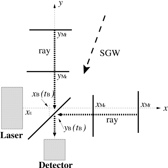
(b)

FIG. 3.: The definitions of various quantities for DL and FP interferometric detectors. (a) A configuration in the absence of gravitational waves. (b) A schematic configuration in the presence of scalar gravitational waves.

FIG. 4.: The frequency response function of FP interferometric detectors at $\theta=\pi/2$ and $\varphi=0$ as a function of $\omega$. In this figure, we adopt the units in which $L$ is unity. The solid, dashed, and dotted lines denotes for $\rho_{\rm M}=0.988$, 0.900 and 0.770, respectively. For $\rho_{\rm M}=0.770$, the same sensitivity becomes almost same as that for Michelson interferometric detectors.

REFERENCES

• [1] S. Nagano, Proc. 2nd TAMA Workshop (Tokyo, Japan, 1999): Gravitational Wave Detection II, eds. S. Kawamura and N. Mio (2000) p.89; M. Ando, ibid., p.101; D. Tatsumi et al., ibid., p.113; S. Telada et al., ibid., p.129; N. Kanda et al., ibid., p.137; H. Tagoshi et al., ibid., p.145; R. Takahashi, ibid., p.151.
• [2] H. Tagoshi, et al., in preparation.
• [3] A. Abramovici et al., Science 256, 325 (1992).
• [4] C. Bradaschia et al., Nucl. Instrum. and Methods A289, 518 (1990).
• [5] J.Hough, in Proceedings of Sixth Marcel Grossman Meeting, ed. by H. Sato and T. Nakamura (World Scientific, Singapore, 1992), p.192.
• [6] LISA Science Team, Laser Interferometer Space Antenna for the detection and observation of gravitational waves: Pre-Phase A Report, Dec. 1995.
• [7] C. M. Will, Theory and experiment in gravitational physics, revised edition (Cambridge University Press, 1993).
• [8] P.G. Bergmann, Int. J. Theor. Phys. 1, 25 (1968).
• [9] R.V. Wagoner, Phys. Rev. 1, 3209 (1970).
• [10] T. Damour and A.M. Polyakov, Nucl. Phys.B423, 532 (1994).
• [11] M. Shibata, K. Nakao and T. Nakamura, Phys. Rev. D50, 7304 (1994).
• [12] T. Harada, T. Chiba, K. Nakao and T. Nakamura, Phys. Rev. D55, 2024 (1997).
• [13] J. Novak, Phys. Rev. D57, 4789 (1998).
• [14] Eubanks et al., Bull. Am. Phys. Soc., Abstract $\#$K 11.05 (1997); C. M. Will, gr-qc/9811036.
• [15] M. Maggiore and A. Nicolis, gr-qc/9907055.
• [16] M. E. Tobar, T. Suzuki and K. Kuroda, Phys. Rev. D59 (1999), 102002; in this article, it was shown that two Fox-Smith interferometric detectors can distinguish the scalar mode from tensor mode.
• [17] B. F. Schutz and C. M. Will, Astrophys. J. Lett. 291, L33 (1985).
• [18] M. Saijo, H. Shinkai, and K. Maeda, Phys. Rev. D 56, 785 (1997).
• [19] R. M. Wald, General Relativity (The University of Chicago Press, 1984).
• [20] R. Schilling, Classical and Quantum Grav. 14, 1513 (1997).