Numerical evolution of Brill waves

Abstract

We report a numerical evolution of axisymmetric Brill waves. The numerical algorithm has new features, including (i) a method for keeping the metric regular on the axis and (ii) the use of coordinates that bring spatial infinity to the edge of the computational grid. The dependence of the evolved metric on both the amplitude and shape of the initial data is found.

]

I Introduction

In the last decade, there has been much use of numerical simulations to study gravitational collapse. These studies include critical collapse[3, 4], black hole collisions[5, 6, 7] and the approach to the singularity[8, 9, 10, 11]. In simulations, spherical or planar symmetry allows the finest resolution, while complete lack of symmetry (a full 3+1 simulation) would allow one to treat a completely general situation. An intermediate case is axisymmetry, which allows more resolution than a full 3+1 simulation; but also permits the study of situations (e.g. prolate collapse or black hole collisions) that do not occur in spherical symmetry.

One issue that can be addressed in axisymmetry is weak cosmic censorship: whether the singularities formed in gravitational collapse are hidden inside black hole event horizons. A simulation done by Shapiro and Teukolsky[12] of the collapse of collisionless matter indicates that weak cosmic censorship may be violated in the collapse of highly prolate objects. The result of reference[12] is that for highly prolate initial configurations, a singularity forms before an apparent horizon. This result might still be consistent with weak cosmic censorship if it is an artifact of the slicing[13] or the type of matter used. To address the second possibility, one would like to know whether the same type of behavior occurs in vacuum collapse.

In [14] Abrahams et al examine families of initial data for Brill waves.[15] These are vacuum, axisymmetric initial data at a moment of time symmetry. The authors of [14] show that by considering sufficiently prolate configurations, one can find initial data with no apparent horizon but with large values of the Riemann invariant ${R^{abcd}}{R_{abcd}}$. They conjecture that such initial data, when evolved, will form singularities without apparent horizons.

In order to test this conjecture, one would like to evolve initial data for highly prolate Brill waves to find the behavior of the evolved spacetime. More generally, one would like to know how the collapse process depends on both the shape and the strength of the initial data. In this paper, we report numerical simulations of the collapse of Brill waves. We find the dependence of the collapse on the amplitude and the initial shape of the wave. The numerical method is presented in section 2 and the results in section 3. Conclusions are given in section 4.

II Numerical method

One difficulty present in numerical simulations of axisymmetric spacetimes is the existence of the axis where the Killing field vanishes. If one chooses coordinates adapted to the symmetry, then there is a coordinate singularity on the axis. This coordinate singularity has the possibility of causing numerical problems: that is, one must be very careful in the choice of numerical method to ensure that the metric remains smooth on the axis. Most axisymmetric simulations use spherical coordinates. In addition to a coordinate singularity on the axis, spherical coordinates lead to a more severe coordinate singularity at the origin. This singularity is either avoided by using initial data with a black hole and no origin,[5] or treated by using elaborate numerical methods to keep the metric regular at the origin.[16]

We bypass this origin difficulty by the use of cylindrical coordinates $(z,r,\phi)$. The spatial metric ${\gamma_{ab}}$ takes the form

$$d{s^{2}}={\psi^{4}}\left[{e^{2rS}}\left(d{z^{2}}+d{r^{2}}\right)+{r^{2}}d{\phi^{2}}\right]$$ (1)

Here, $\psi$ and $S$ are functions of $z,\,r$ and the time $t$. The axis is at $r=0$ and is the only coordinate singularity.

Numerically, the axis is an edge of the computational grid, and therefore values for the variables must be given on the axis points. However, analytically the axis consists of interior points, and therefore the only permissable condition to impose is smoothness. For a scalar $f$, smoothness requires that $f$ be an even function of $r$ and therefore that ${\partial_{r}}f$ vanish on the axis. This condition can be used numerically to set the value of $f$ at the axis points. Similarly, for components of tensors in cylindrical coordinates, smoothness requires either that the component be an even function of $r$ or that it be an odd function of $r$. Odd functions of $r$ vanish on the axis, while even functions have vanishing $r$ derivative on the axis. In either case this information can be used to set the value of the variable at the axis points.

Unfortunately, a difficulty arises because smoothness requires that certain quantities be even and also vanish on the axis. One such quantity is ${{K^{r}}_{r}}-{{K^{\phi}}_{\phi}}$. This quantity must both vanish and have vanishing derivative on the axis. However, since we can impose only one boundary condition at the edge of the computational grid, we do not have a way to maintain both conditions. Our solution to this difficulty is to introduce a new variable: define $W\equiv({{K^{r}}_{r}}-{{K^{\phi}}_{\phi}})/r$. Then $W$ is odd and smoothness requires only that $W$ vanish on the axis. This method is the reason that the term in the exponential in equation (1) is written as $2rS$. Smoothness of the spatial metric requires that ${\gamma_{\phi\phi}}/({r^{2}}{\gamma_{rr}})=1+o({r^{2}})$ and therefore that the quantity $rS$ both vanish and have vanishing derivative on the axis. This condition is met if $S$ vanishes on the axis. In the end, all quantities we deal with either vanish on the axis or have vanishing derivative there, but not both. If we encounter a quantity $f$ that is order $r^{2}$ at the axis, we simply define the odd quantity $g=f/r$ and rewrite all equations containing $f$ in terms of $g$.

There remains the question of how to numerically implement the appropriate conditions on the axis points. For an odd quantity $X$, the most natural method would be to put the first grid point at $r=0$ and impose the condition $X(1)=0$. However, for an even quantity $Y$, the simple condition $Y(1)=Y(2)$ would then impose ${\partial_{r}}Y=0$ not on the axis but at $r={\Delta_{r}}/2$ where $\Delta_{r}$ is the grid spacing in $r$. Instead we use the method of “ghost zones”: the first grid point is at $r=-{\Delta_{r}}/2$. The axis is then halfway between gridpoints 1 and 2. For an odd quantity $X$, we impose the condition $X(1)=-X(2)$ while for an even quantity $Y$, we use $Y(1)=Y(2)$. In each case, the appropriate condition is satisfied on the axis.

We note that our method is not the only way to keep the axis stable. The “cartoon” method of reference[17] begins with a cartesian 3+1 code and operates it in a thin slab with boundary conditions at the faces of the slab given by the axisymmetry of the solution. This cartoon method is effective (see reference[18] for another implementation). However, since a 3+1 code uses more variables than an axisymmetric code, for a given axisymmetric problem the cartoon method uses more computer memory than our method.

We now turn to the method of evolution. The spatial metric $\gamma_{ab}$ is evolved using the ADM equation

$${\partial_{t}}{\gamma_{ab}}=-2\alpha{K_{ab}}+{{\cal L}_{\beta}}{\gamma_{ab}}$$ (2)

where $K_{ab}$ is the extrinsic curvature, $\alpha$ is the lapse and $\beta^{a}$ is the shift. From the form of the metric in equation (1) it is clear that we have imposed the conditions ${\gamma_{rz}}=0$ and ${\gamma_{rr}}={\gamma_{zz}}$. In order that these conditions be preserved by the evolution in equation (2), the shift must satisfy

$${\partial_{r}}{\beta^{z}}+{\partial_{z}}{\beta^{r}}=2\alpha{{K^{z}}_{r}}$$ (3)

$${\partial_{z}}{\beta^{z}}-{\partial_{r}}{\beta^{r}}=\alpha U$$ (4)

where $U\equiv{{K^{z}}_{z}}-{{K^{r}}_{r}}$. This gives rise to the equations

$${\partial_{r}}{\partial_{r}}{\beta^{r}}+{\partial_{z}}{\partial_{z}}{\beta^{r}}=2{\partial_{z}}(\alpha{{K^{z}}_{r}})-{\partial_{r}}(\alpha U)$$ (5)

$${\partial_{r}}{\partial_{r}}{\beta^{z}}+{\partial_{z}}{\partial_{z}}{\beta^{z}}=2{\partial_{r}}(\alpha{{K^{z}}_{r}})+{\partial_{z}}(\alpha U)$$ (6)

Equation (2) yields the following evolution equation for $S$

$${\partial_{t}}S=-\alpha W+{\beta^{z}}{\partial_{z}}S+{\beta^{r}}{\partial_{r}}S+{\beta^{r}}S/r+{\partial_{r}}({\beta^{r}}/r)$$ (7)

where $W\equiv({{K^{r}}_{r}}-{{K^{\phi}}_{\phi}})/r$. Rather than evolve $\psi$, we solve for it using the Hamiltonian constraint.

We choose maximal slicing ($K=0$) and evolve the extrinsic curvature using the ADM equation

$${\partial_{t}}{{K^{a}}_{b}}=-{D^{a}}{D_{b}}\alpha+\alpha{{R^{a}}_{b}}+{{\cal L}_{\beta}}{{K^{a}}_{b}}$$ (8)

where $R_{ab}$ is the Ricci tensor of the spatial metric. Since $K=0$, the only independent components of the extrinsic curvature are ${{K^{z}}_{r}},\,U$ and $W$. These evolve as follows:

$${\partial_{t}}{{K^{z}}_{r}}={\psi^{-4}}{e^{-2rS}}\left[\left(S+2{\psi^{-1}}{\partial_{r}}\psi+r{\partial_{r}}S\right){\partial_{z}}\alpha\right.$$ (9)

$$\left.-{\partial_{z}}{\partial_{r}}\alpha+\left(2{\psi^{-1}}{\partial_{z}}\psi+r{\partial_{z}}S\right){\partial_{r}}\alpha+\alpha{R_{zr}}\right]$$ (10)

$$+{\beta^{z}}{\partial_{z}}{{K^{z}}_{r}}+{\beta^{r}}{\partial_{r}}{{K^{z}}_{r}}+{1\over 2}U\left({\partial_{r}}{\beta^{z}}-{\partial_{z}}{\beta^{r}}\right)$$ (11)

$${\partial_{t}}U={\psi^{-4}}{e^{-2rS}}\left[\left(4{\psi^{-1}}{\partial_{z}}\psi+2r{\partial_{z}}S\right){\partial_{z}}\alpha\right.$$ (12)

$$-\left(2S+4{\psi^{-1}}{\partial_{r}}\psi+2r{\partial_{r}}S\right){\partial_{r}}\alpha$$ (13)

$$\left.+{\partial_{r}}{\partial_{r}}\alpha-{\partial_{z}}{\partial_{z}}\alpha-\alpha{R_{a}}\right]$$ (14)

$$+{\beta^{z}}{\partial_{z}}U+{\beta^{r}}{\partial_{r}}U+2{{K^{z}}_{r}}\left({\partial_{z}}{\beta^{r}}-{\partial_{r}}{\beta^{z}}\right)$$ (15)

$${\partial_{t}}W={\psi^{-4}}{e^{-2rS}}\bigl{[}-{\partial_{r}}\left({r^{-1}}{\partial_{r}}\alpha\right)-{\partial_{z}}S{\partial_{z}}\alpha$$ (16)

$$+\left(S/r+{\partial_{r}}S+4{{(r\psi)}^{-1}}{\partial_{r}}\psi\right){\partial_{r}}\alpha\bigr{]}$$ (17)

$$+\alpha{R_{b}}+{\beta^{z}}{\partial_{z}}W+{\beta^{r}}{\partial_{r}}W+W{\beta^{r}}/r$$ (18)

$$+({{K^{z}}_{r}}/r)\left({\partial_{r}}{\beta^{z}}-{\partial_{z}}{\beta^{r}}\right)$$ (19)

Here we have ${R_{a}}\equiv{R_{rr}}-{R_{zz}}$ and ${R_{b}}\equiv({{R^{r}}_{r}}-{{R^{\phi}}_{\phi}})/r$.

The evolution must preserve the condition $K=0$, which implies that the lapse must satisfy ${D_{a}}{D^{a}}\alpha=\alpha{{K^{a}}_{b}}{{K^{b}}_{a}}$. This equation becomes

$${r^{-1}}{\partial_{r}}\left(r{\psi^{2}}{\partial_{r}}\alpha\right)+{\partial_{z}}\left({\psi^{2}}\;{\partial_{z}}\alpha\right)$$ (20)

$$=\alpha{\psi^{6}}{e^{2rS}}\left[{2\over 3}({U^{2}}+{r^{2}}{W^{2}}+UrW)\,+\,2{{({{K^{z}}_{r}})}^{2}}\right]$$ (21)

The Hamiltonian constraint, $R-{{K^{a}}_{b}}{{K^{b}}_{a}}=0$ becomes the following equation for the conformal factor $\psi$.

$$({\partial_{r}}{\partial_{r}}+{r^{-1}}{\partial_{r}}+{\partial_{z}} {\partial_{z}} )\psi$$ (22)

$$=-(\psi/4)\biggl{[}({\partial_{r}}{\partial_{r}}+{\partial_{z}} {\partial_{z}} )(rS)$$ (23)

$$+{\psi^{4}}{e^{2rS}}\biggl{(}{1\over 3}({U^{2}}+{r^{2}}{W^{2}}+Ur W )+{{({{K^{z}}_{r}})}^{2}}\biggr{)}\biggr{]}$$ (24)

Our set of variables is then ($S,\psi,{{K^{z}}_{r}},U,W,\alpha,{\beta^{r}},{\beta^{z}}$). Of these variables, $S,{{K^{z}}_{r}},W$ and $\beta^{r}$ are odd functions of $r$, while the rest are even functions. These variables are evolved as follows: $S$ and the extrinsic curvature variables are evolved using equations (7,11,15,19). At each time step, the elliptic equations (5,6,21,22) are solved for the shift, lapse and conformal factor.

To begin the evolution, we need initial data satisfying the constraint equations. Initial data for Brill waves is a moment of time symmetry, so ${K_{ab}}=0$ and therefore the momentum constraint is automatically satisfied. The variable $S$ can be freely specified (subject to smoothness on the axis and asymptotic flatness at infinity). Our choice for $S$ is

$$S=ar\exp\left[-{{r^{2}}\over{\sigma_{r}^{2}}}-{{z^{2}}\over{\sigma_{z}^{2}}}\right]$$ (25)

where $a,\,{\sigma_{r}}$ and $\sigma_{z}$ are constants. Here, $a$ is the amplitude of the wave and $\sigma_{r}$ and $\sigma_{z}$ are widths in the $r$ and $z$ directions respectively. Given $S$, equation (22) is solved for $\psi$.

There remains the question of the boundary conditions to apply at the outer edge of the computational grid. A natural method would be to put the outer edge of the computational grid at some large distance and to impose some outgoing wave condition on the evolution equations and a Robin boundary condition on the elliptic equations. However, the issue of appropriate boundary conditions for a mixed hyperbolic-elliptic set of equations is quite complicated. This issue becomes even more dificult in cylindrical coordinates than in spherical coordinates since the asymptotic behavior of the variables looks more complicated in cylindrical coordinates. Our attempts to impose a boundary condition of this sort led to numerical instability. Instead, we decided to use a different approach. We begin by noting that a coordinate transformation can bring spatial infinity to the edge of the computational grid. We introduce new coordinates $({\tilde{z}},{\tilde{r}})$ defined by $z=\tan{\tilde{z}}$ and $r=\tan{\tilde{r}}$. We then place the edges of the computational grid at ${\tilde{z}}=\pi/2$ and at ${\tilde{r}}=\pi/2$. These regions correspond to spatial infinity. Though we use new coordinates, we retain the old metric and extrinsic curvature variables, with the exception that we introduce the quantities ${\tilde{S}}=S/\cos{\tilde{r}}$ and ${\tilde{W}}=W/\cos{\tilde{r}}$. Thus our set of variables is $({\tilde{S}},\psi,{{K^{z}}_{r}},U,{\tilde{W}},\alpha,{\beta^{r}},{\beta^{z}})$ and the set of equations used to evolve these variables is equations (7,11,15,19,5, 6,21,22) with the substitutions $r\to\tan{\tilde{r}},{\partial_{r}}\to{\cos^{2}}{\tilde{r}}{\partial_{\tilde{r}}},\,{\partial_{z}}\to{\cos^{2}}{\tilde{z}}{\partial_{\tilde{z}}},\,S\to\cos{\tilde{r}}{\tilde{S}}$ and $W\to\cos{\tilde{r}}{\tilde{W}}$.

Since the edge of the grid is at spatial infinity, the choice of boundary condition is dictated by asymptotic flatness: $\psi$ and $\alpha$ must be 1 at the outer boundary, and all the other variables must vanish there. Though the coordinate transformation is singular, this does not lead to a singularity in the evolution equations. In fact, just the opposite is true: in the new coordinates, the right hand sides of the evolution equations approach zero at spatial infinity (as they must, since the variables are unchanging there).

The advantages of this spatial infinity boundary condition are stability and consistency with the field equations. However, there are disadvantages as well. The change of variables changes the form of the elliptic operators that need to be inverted to solve the elliptic equations. This slows down the process of solving the elliptic equations and therefore slows down the code. A more fundamental difficulty has to do with waves produced in the collapse process. As a wave travels outward, its (approximately constant) physical width corresponds to fewer coordinate grid spacings. Eventually, the wave fails to be resolved, and since the system is mixed hyperbolic-elliptic, this failure of resolution in one part of the grid can affect the entire grid. This difficulty means that for a given spatial resolution, there is only a certain amount of time that the evolution can be run and still give reliable results. This places a limit on the type of problems that can be treated using this method.

The variables $({\tilde{S}},{{K^{z}}_{r}},U,{\tilde{W}})$ are evolved using a 3 step iterative Crank-Nicholson (ICN) algorithm. At each step of the ICN process, the elliptic equations for $(\psi,\alpha,{\beta^{r}},{\beta^{z}})$ are solved using the conjugate gradient method with Neumann preconditioning.

Though we solve for $\psi$ using the Hamiltonian constraint, we note that $\psi$ also satisfies an evolution equation. From equation (2) we have

$${\partial_{t}}\psi={\beta^{z}}{\partial_{z}}\psi+{\beta^{r}}{\partial_{r}}\psi+\psi\left[{{\beta^{r}}\over{2r}}+{\alpha\over 6}(U+2rW)\right]$$ (26)

We use equation (26) as a check on the reliability of the code. Specifically, we compute a second value of $\psi$ by starting with the initial data and then evolving using equation (26). We then check that the two values of $\psi$ agree well at $r=z=0$. We run the code only as long as this good agreement persists.

The convergence of the code is tested using the momemtum constraint ${p_{a}}={D^{b}}{K_{ab}}$ (Since $K=0$). The Hamiltonian constraint is solved for $\psi$ and therefore cannot be used as an independent test. In general, the methods we use would lead one to expect second order convergence. However, the boundary conditions at infinity for the elliptic equations may be only first order accurate. Figure 1 shows the ${\rm L}^{2}$ norm of $p_{z}$ plotted as a function of time. For these runs, $a=4$ and ${\sigma_{r}}={\sigma_{z}}=1$. The dashed line corresponds to 42 gridpoints in the $r$ direction and 42 gridpoints in the $z$ direction, while the solid line corresponds to a run with twice the resolution. The results indicate second order convergence.

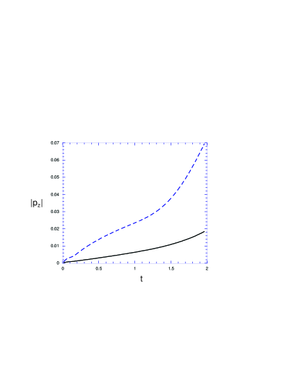
FIG. 1.: $|{p_{z}}|$ plotted vs. $t$ for two different resolutions

III Results

The code was run in double precision on Dec alpha workstations and on the NCSA Origin 2000. Unless otherwise stated, all simulations were run with 42 gridpoints in the $r$ direction and 42 gridpoints in the $z$ direction.

The initial data that we use, and therefore the spacetime that it evolves to, has reflection symmetry about the $z=0$ plane. Though our algorithm does not require this extra symmetry, since the spacetimes we treat have this reflection symmetry, we save computational time by running the simulations in the range $0\leq{\tilde{z}}<\pi/2$. The reflection symmetry and axisymmetry give spacetime a preferred world line: the origin ($r=z=0$). In gravitational collapse in maximal slicing, it is expected that the lapse approaches zero in the region of strong gravity. Therefore, a useful quantity to plot is $\ln{\alpha_{0}}$ as a function of time, where $\alpha_{0}$ is the lapse at the origin. Note that this quantity can be directly compared between two different codes, provided that both use maximal slicing.

Our initial data has three parameters: the amplitude $a$ and the two widths $\sigma_{r}$ and $\sigma_{z}$. However, it turns out that the effective parameter space is two dimensional. Under the transformation ${\sigma_{r}}\to c{\sigma_{r}},\;{\sigma_{z}}\to c{\sigma_{z}},\;a\to a/{c^{2}}$ for a positive constant $c$, the spacetime is changed only by an overall constant scale. We can think of the two remaining parameters as being the strength and shape of the wave, and we want to find the dependence of the collapse on these two parameters. Figure 2 shows the dependence of the collapse on the strength of the wave. Here, three simulations are run, each with ${\sigma_{r}}={\sigma_{z}}=1$. The parameter $a$ is $4$ for the solid line, $5$ for the dashed line and $6$ for the dot-dashed line. The $a=4$ and $a=6$ spacetimes have been studied using a 3+1 code in reference[19]. Our results are in good agreement with theirs. For $a=4$, the lapse, after an initial collapse to small values, appears to be returning to 1. That is, we expect the Brill wave to disperse. For $a=6$, the lapse continues to collapse, and we expect a black hole to form. Somewhere between $a=4$ and $a=6$ is an amplitude that leads to critical collapse; however our method does not have the resolution needed to study this process. The reason for this is that to study critical collapse, one must evolve long enough to distinguish a spacetime slightly below the black hole threshold from one that is slightly above. In this amount of time, the waves traveling towards the outer boundary will, in general fail to be resolved, leading to a general lack of accuracy in the results of the evolution.

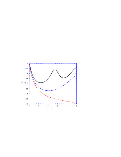
FIG. 2.: $\ln{\alpha_{0}}$ plotted vs. $t$ for three different amplitudes: $a=4$ (solid line), $a=5$ (dashed line) and $a=6$ (dot-dashed line)

The issue of the dependence of the collapse process on the shape is somewhat subtle, due to the question of what is to be held constant as the shape varies. The simplest thing to do is to hold the amplitude $a$ and the sum ${\sigma_{r}}+{\sigma_{z}}$ constant while varying ${\sigma_{r}}-{\sigma_{z}}$. Results of these collapse simulations are shown in figure 3. Here, $a=4$ and ${\sigma_{r}}+{\sigma_{z}}=2$ for all simulations. We will call initial data “spherical” if ${\sigma_{r}}={\sigma_{z}}$, “prolate” if ${\sigma_{r}}<{\sigma_{z}}$ and “oblate” if ${\sigma_{r}}>{\sigma_{z}}$. (This terminology is somewhat misleading, since it is not the wave itself but the initial $S/r$ that is spherical, prolate or oblate). Figure 3 contains a spherical collapse (solid line), a prolate collapse (dashed line) with ${\sigma_{r}}-{\sigma_{z}}=-0.4$ and an oblate collapse (dot-dashed line) with ${\sigma_{r}}-{\sigma_{z}}=0.4$. Here the shape seems to have a large influence on the collapse, with even a small amount of oblateness producing collapse, while a small amount of prolateness hastens dispersion.

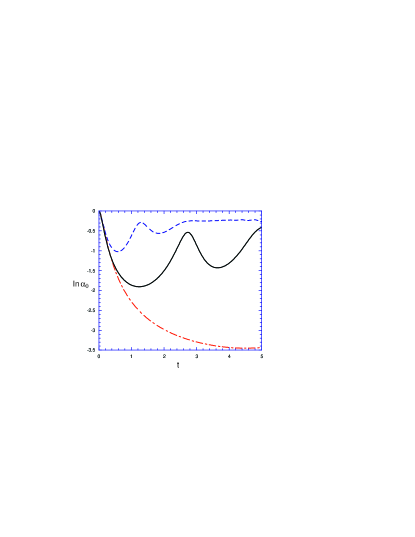
FIG. 3.: $\ln{\alpha_{0}}$ plotted vs. $t$ for $a=4$ and three different shapes: spherical (solid line), prolate (dashed line) and oblate (dot-dashed line)

However, it is not clear how to interpret this result, since for a fixed $a$ and ${\sigma_{r}}+{\sigma_{z}}$, it may be that there is a dependence of the “strength” of the gravitational wave on ${\sigma_{r}}-{\sigma_{z}}$. To see this, we examine how the ADM mass depends on the degree of prolateness or oblateness at fixed $a$ and ${\sigma_{r}}+{\sigma_{z}}$. These results are shown in figure 4. Here, we have ${\sigma_{r}}+{\sigma_{z}}=2$ and $a=4$. The ADM mass $M$ is plotted as a function of ${\sigma_{r}}/{\sigma_{z}}$. Since, at a fixed $a$, $M$ is an increasing function of ${\sigma_{r}}/{\sigma_{z}}$, this is (at least part of) the reason why at fixed $a$ oblateness causes collapse.

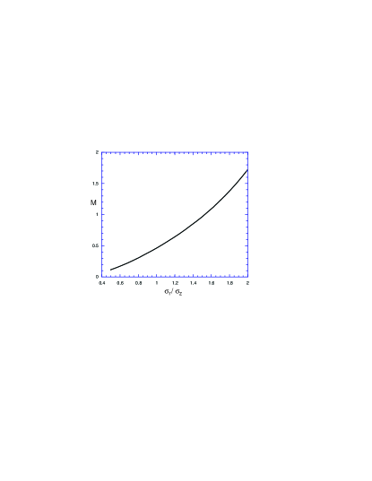
FIG. 4.: $M$ plotted vs. ${\sigma_{r}}/{\sigma_{z}}$ for $a=4$ and ${\sigma_{r}}+{\sigma_{z}}=2$

One might therefore instead look at the influence of shape at fixed ${\sigma_{r}}+{\sigma_{z}}$ and fixed $M$. The results of this comparison are shown in figure 5. Here ${\sigma_{r}}+{\sigma_{z}}=2$ and $M=0.46$ (the value of $M$ corresponding to $a=4$ and ${\sigma_{r}}={\sigma_{z}}=1$). The solid line is a spherical collapse, while the dashed line is a prolate collapse with ${\sigma_{r}}-{\sigma_{z}}=-0.4$ (corresponding to $a=6.1$) and the dot-dashed line is an oblate collapse with ${\sigma_{r}}-{\sigma_{z}}=0.4$ (corresponding to $a=2.7$). Here the shape has some influence on the details of the collapse process; but this much change in the shape does not seem to have a particular tendency either to promote or to inhibit collapse. Figure 6 shows the same sort of plot, but with more distortion in the shape. Again $M=0.46$ and ${\sigma_{r}}+{\sigma_{z}}=2$. However, here the prolate collapse (dashed line) has ${\sigma_{r}}-{\sigma_{z}}=-1$ ($a=14$) and the oblate collapse (dot-dashed line) has ${\sigma_{r}}-{\sigma_{z}}=1$ ($a=1.4$) in addition to the spherical collapse (solid line). Here it seems that at constant ADM mass there is a slight tendency of oblateness to induce dispersion.

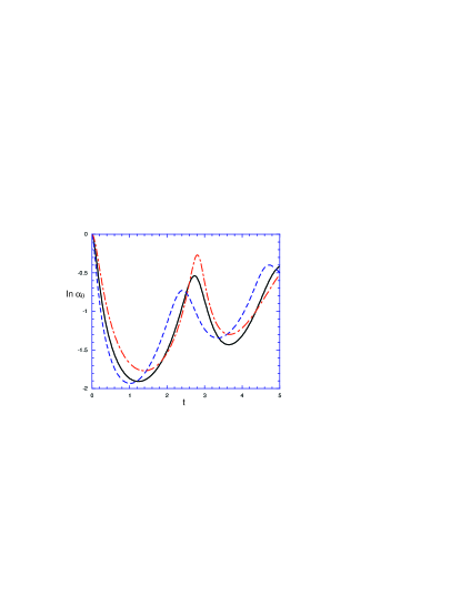
FIG. 5.: $\ln{\alpha_{0}}$ plotted vs. $t$ for $M=0.46$ and three different shapes: spherical (solid line), prolate (dashed line) and oblate (dot-dashed line)

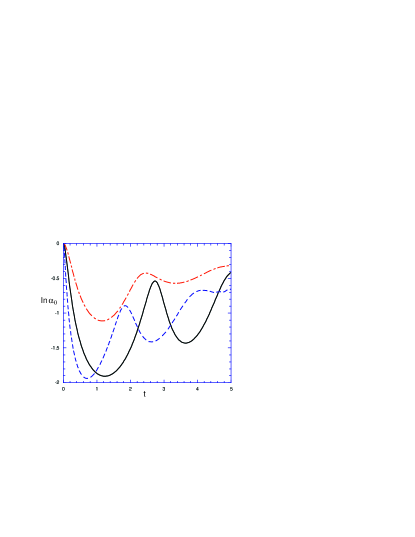
FIG. 6.: $\ln{\alpha_{0}}$ plotted vs. $t$ for $M=0.46$ and three different shapes: spherical (solid line), prolate (dashed line) and oblate (dot-dashed line). Here the amount of oblateness or prolateness is greater than that in figure 4

We now consider more strongly gravitating initial data and follow its evolution until the formation of an apparent horizon, while considering some of the properties of the collapse. This simulation has $M=2,\,{\sigma_{r}}=1$ and ${\sigma_{z}}=1$ ($a=8.5$) and is run with 82 gridpoints in the $r$ direction and 82 gridpoints in the $z$ direction. Figure 7 shows $\ln{\alpha_{0}}$ as a function of time. The lapse collapses throughout the evolution. At each time step we calculate the Riemann invariant $I={R^{abcd}}{R_{abcd}}/16$ and find the maximum of its absolute value $I_{\rm max}$ as well as the spatial position where $|I|={I_{\rm max}}$. Figure 8 shows $\ln{I_{\rm max}}$ plotted as a function of time. Here we see that after an initial increase, $\ln{I_{\rm max}}$ decreases during the rest of the evolution. At all times during the evolution the place where $|I|={I_{\rm max}}$ is the origin.

To monitor the approach to apparent horizon formation, we consider how the horizon is found. On a maximal slice in an axisymmetric spacetime, the horizon is given by a curve $z=f(r)$ where the function $f$ satisfies a differential equation that is integrated from the axis to $z=0$. Let $\theta$ denote the angle at which the curve meets the $z=0$ plane. Then the curve is a horizon only if $\theta=\pi/2$. The horizon finding subroutine integrates the differential equation for $f$ starting at each point on the axis, finds the angle $\theta$ for each curve and then finds $\theta_{\rm max}$, the maximum value over all curves of this angle. If ${\theta_{\rm max}}<\pi/2$ then there is no horizon at this time. Figure 9 shows $2{\theta_{\rm max}}/\pi$ plotted as a function of time. Note that $\theta_{\rm max}$ increases throughout the collapse process. Note also that even before the actual horizon formation, one can tell that a horizon is about to form by noticing that $\theta_{\rm max}$ is approaching $\pi/2$. The horizon forms at $t=3.9$ with area $A=165=0.82(16\pi{M^{2}})$.

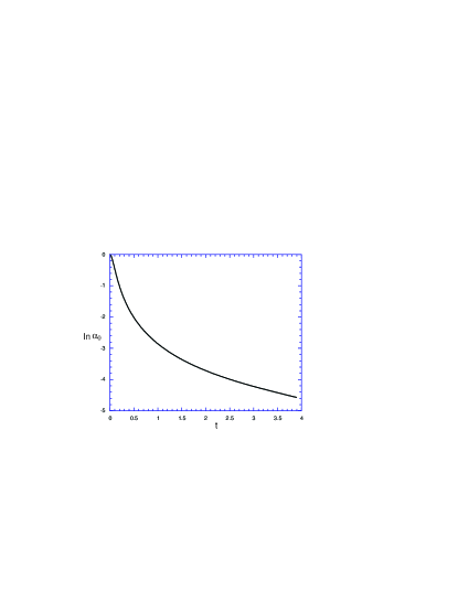
FIG. 7.: $\ln{\alpha_{0}}$ plotted vs. $t$ for $M=2$ and ${\sigma_{r}}={\sigma_{z}}=1$

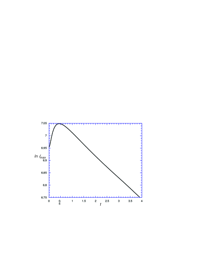
FIG. 8.: $\ln{I_{\rm max}}$ plotted vs. $t$ for $M=2$ and ${\sigma_{r}}={\sigma_{z}}=1$

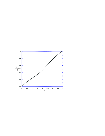
FIG. 9.: $2{\theta_{\rm max}}/\pi$ plotted vs. $t$ for $M=2$ and ${\sigma_{r}}={\sigma_{z}}=1$

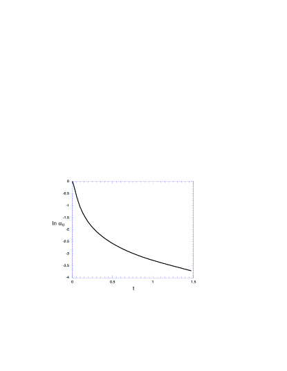
FIG. 10.: $\ln{\alpha_{0}}$ plotted vs. $t$ for $M=2,\,{\sigma_{r}}=0.128$ and ${\sigma_{z}}=1.6$

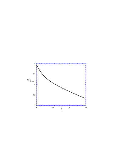
FIG. 11.: $\ln{I_{\rm max}}$ plotted vs. $t$ for $M=2,\,{\sigma_{r}}=0.128$ and ${\sigma_{z}}=1.6$

We now turn to a highly prolate collapse: the evolution of one of the initial data sets of reference[14]. Here, $M=2,\,{\sigma_{z}}=1.6$ and ${\sigma_{r}}=0.128$ ($a=325$). This simulation was run with 162 grid points in the $r$ direction and 42 grid points in the $z$ direction. Ideally, we would like to follow the collapse until either a horizon forms or a curvature scalar blows up. Unfortunately, we are not able to follow the evolution that long; so we evolve for a somewhat shorter time and attempt to discern trends in the evolution. Figure 10 shows $\ln{\alpha_{0}}$ plotted as a function of time. Here we see the usual collapse of the lapse throughout the evolution. Figure 11 shows $\ln{I_{\rm max}}$ plotted as a function of time. Here we see that the maximum of the Riemann invariant decreases as the collapse proceeds. In the initial data, the spatial location where $|I|={I_{\rm max}}$ is on the axis at $z=1.04$. As the evolution proceeds, this spatial location remains on the axis, but moves towards the origin, reaching the origin at $t=0.55$ and then remaining at the origin for the rest of the evolution. To discern a trend in the approach to apparent horizon formation, we plot (Figure 12) $2{\theta_{\rm max}}/\pi$ as a function of time for this simulation. Note that this quantity is increasing.

The trends of this evolution are that (i) $I_{\rm max}$ decreases, (ii) the spatial position where $|I|={I_{\rm max}}$ moves to the origin and (iii) $\theta_{\rm max}$ increases. If these trends continue, then this spacetime will form a black hole rather than a naked singularity. Thus (in this example at least) it seems that Brill waves behave differently from collisionless matter with even highly prolate initial configurations forming black holes. This conclusion is not firm for two reasons: (i) we have only followed the evolution for a certain amount of time, and the trends that we have observed in this part of the evolution could reverse in later parts. (ii) we have only evolved a certain, highly prolate initial configuration. It is possible that much more prolate initial configurations behave differently. Both these issues need further study.

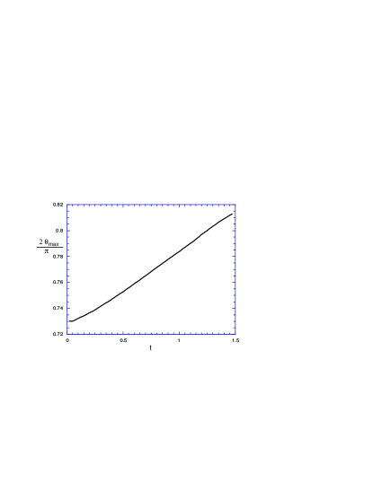
FIG. 12.: $2{\theta_{\rm max}}/\pi$ plotted vs. $t$ for $M=2,\,{\sigma_{r}}=0.128$ and ${\sigma_{z}}=1.6$

IV Conclusion

We have presented (i) a new method of curing axis instabilities, (ii) a study of the dependence of Brill wave collapse on the shape of the wave including (iii) a preliminary examination of the issue of cosmic censorship in the collapse of highly prolate Brill waves. A convincing demonstration that the axis really is stable would require evolution for long times. However, our outer boundary condition entails a loss of resolution that increases with time and this prevents us from running the code for a long time, even for weak waves. (Note: one might also expect that our sort of outer boundary condition would result in spurious reflected waves. While we cannot run our code long enough to check this, we have used our outer boundary condition to perform a numerical simulation of the linear wave equation; and there we find very little reflection).

A way to test the regular axis method independently of the question of outer boundary conditions is to treat the case of closed cosmologies. One of us has used the regular axis method to treat Gowdy spacetimes on ${S^{2}}\times{S^{1}}\times R$.[20] Here the evolution proceeds for long times and there is no axis instability. Though the Gowdy spacetimes have two Killing fields, one can easily apply the regular axis method to closed axisymmetric cosmologies.

To do a more thorough study of Brill wave collapse, we require a better way of treating the outer boundary. One way to do this is to put the boundary at a finite distance but replace the ADM system by one in which a simple outgoing wave boundary condition does not cause numerical instability. The method of Baumgarte, Shapiro, Shibata and Nakamura[21, 22] seems to have the appropriate properties. Another method would use harmonic coordinates, which makes Einstein’s equation similar to the wave equation and should be stable with an outgoing wave boundary condition. Alternatively, one could keep spatial infinity (or null infinity) on the computational grid, but replace the ADM equations with the conformal equations of Friedrich.[23, 24, 25] We are presently examining these alternatives to see which is likely to work best for Brill wave simulations.

Our preliminary results on Brill wave collapse indicate that even highly prolate Brill waves do not evolve to form naked singularities. In the evolution of highly prolate initial data, gravitational collapse will tend to increase the Riemann curvature, while the tendency of the wave to spread out will lessen curvature. We have shown that in the initial stage of the evolution of a highly prolate wave, the second effect is the more important one. That is, the highly prolate wave tends to become less prolate rather than more as it evolves. In this way, Brill waves behave differently from the collisionless matter studied in reference[12]. To put our tentative conclusions on a firmer footing, we need to study more extreme configurations and evolve them for a longer time.

- [1] Email: garfinkl@oakland.edu
- [2] Email: gcd@chandra.bgsu.edu
- [3] M. Choptuik, Phys. Rev. Lett. 70, 9 (1993)
- [4] For a review, see C. Gundlach, Adv. Theor. Phys. 2, 1 (1998) and references therein
- [5] P. Anninos et al, Phys. Rev. Lett. 71, 2851 (1993)
- [6] P. Anninos et al, Phys. Rev. D 52, 2044 (1995)
- [7] P. Anninos and S. Brandt, Phys. Rev. Lett. 81, 508 (1998)
- [8] B. Berger and V. Moncrief, Phys. Rev. D 48, 4676 (1993)
- [9] B. Berger and V. Moncrief, Phys. Rev. D 57, 7235 (1998)
- [10] M. Weaver, J. Isenberg and B. Berger, Phys. Rev. Lett. 80, 2984 (1998)
- [11] B. Berger, D. Garfinkle, J. Isenberg, V. Moncrief and M. Weaver, Mod. Phys. Lett. A 13, 1565 (1998)
- [12] S. Shapiro and S. Teukolsky, Phys. Rev. Lett. 66, 994 (1991)
- [13] V. Iyer and R. Wald, Phys. Rev. D44, 3719 (1991)
- [14] A. Abrahams, K. Heiderich, S. Shapiro and S. Teukolsky, Phys. Rev. D 46, 2452 (1992)
- [15] D. Brill, Ann. Phys. (N.Y.) 7, 466 (1959)
- [16] A. Abrahams and C. Evans, Phys. Rev. D 46, R4117 (1992)
- [17] M. Alcubierre, S. Brandt, B. Bruegmann, D. Holz, E. Seidel, R. Takahashi and J. Thornburg, gr-qc/9908012
- [18] M. Shibata, gr-qc/0007049
- [19] M. Alcubierre, G. Allen, B. Brugman, G. Lanfermann, E. Seidel, W. Suen and M. Tobias, Phys. Rev. D 61, 041501 (2000)
- [20] D. Garfinkle, Phys. Rev. D60, 104010 (1999)
- [21] T. Baumgarte and S. Shapiro, Phys. Rev. D59, 024007 (1999)
- [22] M. Shibata and T. Nakamura, Phys. Rev. D52, 5428 (1995)
- [23] H. Friedrich, Proc. Roy. Soc. 375, 169 (1981)
- [24] H. Friedrich, J. Geom. Phys. 24, 83 (1998)
- [25] P. Huebner, Class. Quant. Grav. 16, 2823 (1999)