Abstract

Gravitational waves (GW) are propagated perturbations of the space-time geometry, and they show up locally as tides, i.e., local gravity gradients which vary with time. These gradients are determined by six often called electric components of the Riemann tensor, which in a local coordinate frame are $R_{0i0j}$, ($i,j=1,2,3$). A GW detector is a device designed to generate information on those quantities on the basis of suitable measurements. Both Weber bars and laser interferometers are single mode antennas, i.e., they generate a single readout which is the result of the combined action of those six GW’s Riemann tensor amplitudes on the system sensor’s output port.

A spherical detector is not limited in that fashion: this is because its degenerate oscillation eigenmodes are uniquely matched to the structure of the above Riemann tensor components. This means that a solid spherical body is a natural multimode GW detector, i.e., it is fully capable of delivering six channel outputs, precise combinations of which completely deconvolve the six GW amplitudes.

The present article is concerned with the theoretical reasons of the remarkable properties of a spherical GW detector. The analysis proceeds from first principles and is based on essentially no ad hoc hypotheses. The mathematical beauty of the theory is outstanding, and abundant detail is given for a thorough understanding of the fundamental facts and ideas. Experimental evidence of the accuracy of the model is also provided, where possible.

Abstract

A general formalism is set up to analyse the response of an arbitrary solid elastic body to an arbitrary metric Gravitational Wave perturbation, which fully displays the details of the interaction wave-antenna. The formalism is applied to the spherical detector, whose sensitivity parameters are thereby scrutinised. A multimode transfer function is defined to study the amplitude sensitivity, and absorption cross sections are calculated for a general metric theory of GW physics. Their scaling properties are shown to be independent of the underlying theory, with interesting consequences for future detector design. The GW incidence direction deconvolution problem is also discussed, always within the context of a general metric theory of the gravitational field.

Abstract

Apart from omnidirectional, a solid elastic sphere is a natural multi-mode and multi-frequency device for the detection of Gravitational Waves (GW). Motion sensing in a spherical GW detector thus requires a multiple set of transducers attached to it at suitable locations. If these are resonant then they exert a significant back action on the larger sphere and, as a consequence, the joint dynamics of the entire system must be properly understood before reliable conclusions can be drawn from its readout. In this paper, I present and develop an analytic approach to study such dynamics which generalises currently existing ones and clarifies their actual range of validity. In addition, the new formalism shows that there actually exist resonator layouts alternative to the highly symmetric TIGA, potentially having interesting properties. One of these (I will call it PHC), which only requires five resonators per quadrupole mode sensed, and has mode channels, will be described in detail. Also, the perturbative nature of the proposed approach makes it very well adapted to systematically assess the consequences of realistic mistunings in the device parameters by robust analytic methods. In order to check the real value of the mathematical model, its predictions have been confronted with experimental data from the LSU prototype detector TIGA, and agreement between both is found to consistently reach a satisfactory precision of four decimal places.

Summary

The following pages contain the fusion of two published papers: What can we learn about gravitational wave physics with an elastic spherical antenna?, published in the Physical Review (PRD 52, 591-604 (1995)), and Multiple mode gravitational wave detection with a spherical antenna, scheduled to appear in the July-2000 issue of Monthly Notices of the Royal Astronomical Society (MNRAS 316, 173-194 (2000)). In them, I first developed an analytic model to describe the interaction of a solid elastic sphere with an incoming flux of gravitational waves of the general metric class, then extended it to also address the multimode signal deconvolution problem by means of suitable layouts of resonant motion sensors.

I think the model is quite complete as regards the major conceptual issues in a spherical GW detector, therefore think merging the two papers together makes positive sense. Let me however stress that I do not mean to understate the fundamental problem of noise, which is here left aside; rather, it is now being actively investigated in detail within the very convenient general framework set up below.

What can we learn about GW Physics … is already five years old, and certain parts of it have been the subject of further research since. More specifically, this happens with Brans-Dicke absorption cross sections, see section 4, where reference has been added to such newer work. In addition, two new tables and more mathematical detail have been added to its Appendix B. The latter should help the interested reader with certain technicalities, while the tables and attendant new formulas are meant to provide explicit numerical values of the frequency spectrum of the sphere rather than the original only graphics information. I expect this to be useful reference in numerical and/or experimental determinations of these quantities.

No changes have been included in the second paper relative to its MNRAS version. In merging the two articles together, however, I have found expedient to renumber the equations and bibliographic references into corresponding single streams. The bibliography has been updated and made into a unique list at the end of the file in alphabetical order. Finally, I have included minor notation changes in order to reconcile otherwise small mistunings between both articles.

Alberto Lobo
                                                                                               Barcelona, June 2000

What can we learn about GW Physics with an elastic spherical antenna?

PRD 52, 591-604 (1995)

José Alberto Lobo

Departament de Física Fonamental

Universitat de Barcelona, Spain

e-mail: lobo@hermes.ffn.ub.es

1 Introduction

Spherical antennae are considered by many to be the natural next step in the development of resonant GW detectors. The reasons for this new trend essentially derive from the improved sensitivity of a sphere —which can be nearly an order of magnitude better than a cylinder having the same resonance frequency, see below and [clo]—, and from its multimode capabilities, first recognised by Forward [fo71] and further elaborated in [wp77, jm93].

Although some of the most relevant aspects of detector sensitivity have already received attention in the literature, it seems to me that a sufficiently general and flexible analysis of the interaction between GW and detector has not been satisfactorily developed to date. This theoretical shortage has a number of practical negative consequences, too. Traditional analysis, to mention but an example, is almost invariably restricted to General Relativity or scalar–tensor theories of gravity; while it may be argued that this is already very general, any such argument is, as a matter of fact, understating the potentialities actually offered by a spherical GW antenna to help decide for or against any one specific theory of the gravitational field on the basis of experimental observation.

I thus propose to develop in this paper a full fledged mathematical formalism which will enable analysis of the antenna’s response to a completely general GW, i.e., making no a priori assumptions about which is the correct theory underlying GW physics (other than, indeed, that it is a metric theory), and also making no assumptions about detector shape, structure or boundary conditions. Considering things in such generality is not only “theoretically nice” —it also brings about new results and a better understanding of older ones. For example, it will be proved that the sphere is the most efficient GW elastic detector shape, and that higher mode absorption cross sections scale independently of GW physics. I will also discuss the direction of incidence deconvolution problem in the context of a general metric theory of gravity.

The paper is organised as follows: section 2 is devoted to the development of the general mathematical framework, leading to a formula in which an elastic solid’s response is related to the action of an arbitrary metric GW impinging on it. In section 3 the general equations are applied to the homogeneous spherical body, and a discussion of the deconvolution problem is presented as well. Section 4 contains the description of the sphere’s sensitivity parameters, specifically leading to the concept of multimode, or vector, transfer function, and to an analysis of the absorption cross section presented by this detector to a passing by GW. Conclusions and prospects are summarised in section 5, and two appendices are added which include mathematical derivations.

2 General mathematical framework

In the mathematical model, I shall be assuming that the antenna is a solid elastic body which responds to GW perturbations according to the equations of classical non-relativistic linear Elasticity Theory [ll70]. This is fully justified because GW-induced displacements will be very small indeed, and the speed of such displacements much smaller than that of light for any foreseeable frequencies. Although our primary interest is a spherical antenna, the considerations which follow in the remainder of this section have general validity for arbitrarily shaped, isotropic elastic solids.

Let ${\bf u}({\bf x},t)$ be the displacement vector of the infinitesimal mass element sitting at point x relative to the solid’s centre of mass in its unperturbed state, whose density distribution in that state is $\varrho$. Let $\lambda$ and $\mu$ be the material’s elastic Lamé coefficients. If a volume force density ${\bf f}({\bf x},t)$ acts on such solid, the displacement field ${\bf u}({\bf x},t)$ is the solution to the system of partial differential equations [ll70]

$$\varrho\frac{\partial^{2}{\bf u}}{\partial t^{2}}-\mu\nabla^{2}{\bf u}-(\lambda+\mu)\,\nabla(\nabla{\bf\cdot}{\bf u})={\bf f}({\bf x},t)$$ (1)

with the appropriate initial and boundary conditions. A summary of notation and general results regarding the solution to that system is briefly outlined in the ensuing subsection, as they are necessary for the subsequent developments in this paper, and also in future work —e.g. page 1 and ss. below.

2.1 Separable driving force

For reasons which will become clear later on, we shall only be interested in driving forces of the separable type

$${\bf f}({\bf x},t)={\bf f}({\bf x})\,g(t)$$ (2)

or, indeed, linear combinations thereof. The solution to (1) does not require us to specify the precise boundary conditions on ${\bf u}({\bf x},t)$ at this stage, but we need to set the initial conditions. We adopt the following:

$${\bf u}({\bf x},0)={\bf\dot{u}}({\bf x},0)=0$$ (3)

where  ${\bf\dot{}}\equiv\partial/\partial t$, implying that the antenna is at complete rest before observation begins at $t$=0. The structure of the force field (2) is such that the displacements ${\bf u}({\bf x},t)$ can be expressed by means of a Green function integral of the form

$${\bf u}({\bf x},t)=\int_{0}^{\infty}{\bf S}({\bf x};t-t^{\prime})\,g(t^{\prime})\,dt^{\prime}$$ (4)

The deductive procedure whereby ${\bf S}({\bf x};t-t^{\prime})$ is calculated can be found in many standard textbooks —see e.g. [tm87]. The result is

$${\bf S}({\bf x};t)=\left\{\begin{array}[]{ll}0&\ \ {\rm if}\ \ t\leq 0\\[10.00002pt] \sum_{N}\,\mbox{\large$\frac{f_{N}}{\omega_{N}}$}\,{\bf u}_{N}({\bf x})\sin\omega_{N}t&\ \ {\rm if}\ \ t\geq 0\end{array}\right.$$ (5)

where

$$f_{N}\equiv\frac{1}{M}\,\int_{\rm Solid}{\bf u}_{N}^{*}({\bf x})\cdot{\bf f}({\bf x})\,d^{3}x$$ (6)

and ${\bf u}_{N}({\bf x})$ are the normalised eigen–solutions to

$$\mu\nabla^{2}{\bf u}_{N}+(\lambda+\mu)\,\nabla(\nabla{\bf\cdot}{\bf u}_{N})=-\omega_{N}^{2}\varrho{\bf u}_{N}$$ (7)

with suitable boundary conditions. Here $N\/$ represents an index, or set of indices, labelling the eigenmode of frequency $\omega_{N}$. The normalisation condition is (arbitrarily) chosen so that

$$\int_{\rm Solid}{\bf u}_{N^{\prime}}^{*}({\bf x})\cdot{\bf u}_{N}({\bf x})\,\varrho({\bf x})\,d^{3}x=M\,\delta_{N^{\prime}N}$$ (8)

where $M\/$ is the total mass of the solid, and the asterisk denotes complex conjugation. Replacing now (5) into (4) we can write the solution to our problem as a series expansion:

$${\bf u}({\bf x},t)=\sum_{N}\,\frac{f_{N}}{\omega_{N}}\,{\bf u}_{N}({\bf x})\,g_{N}(t)$$ (9)

where

$$g_{N}(t)\equiv\int_{0}^{t}g(t^{\prime})\,\sin\omega_{N}(t-t^{\prime})\,dt^{\prime}$$ (10)

Equation (9) is the formal solution to our problem; it has the standard form of an orthogonal expansion and is valid for any solid driven by a separable force like (2) and any boundary conditions. It is therefore completely general, given that type of force.

Before we go on, it is perhaps interesting to quote a simple but useful example. It is the case of a solid hit by a hammer blow, i.e., receiving a sudden stroke at a point on its surface. Exam of the response of a GW antenna to such perturbation is being used for correct tuning and monitoring of the device [wjpc]. If the driving force density is represented by the simple model

$${\bf f}^{({\rm hb})}({\bf x},t)={\bf f}_{0}\,\delta^{(3)}({\bf x}-{\bf x}_{0})\,\delta(t)$$ (11)

where ${\bf x}_{0}$ is the surface point hit, and ${\bf f}_{0}$ is a constant vector, then the system’s response is immediately seen to be

$${\bf u}^{({\rm hb})}({\bf x},t)=\sum_{N}\,\frac{f_{N}^{0}}{\omega_{N}}\,{\bf u}_{N}({\bf x})\sin\omega_{N}t$$ (12)

with $f_{N}^{0}=M^{-1}\,{\bf f}_{0}\!\cdot\!{\bf u}_{N}^{*}({\bf x}_{0})$. A hammer blow thus excites all the solid’s normal modes, except those perpendicular to ${\bf f}_{0}$, with amplitudes which are inversely proportional to the mode’s frequency. This is seen to be a rather general result in the theory of sound waves in isotropic elastic solids.

2.2 The GW tidal forces

An incoming GW manifests itself as a tidal force density; in the long wavelength linear approximation [mtw] it only depends on the “electric” components of the Riemann tensor:

$$f_{i}({\bf x},t)=\varrho c^{2}\,R_{0i0j}(t)\,x_{j}$$ (13)

where $c\/$ is the speed of light, and sum over the repeated index j is understood. In (13) tidal forces are referred to the antenna’s centre of mass, and thus x is a vector originating there. Note that I have omitted any dependence of $R_{0i0j}$ on spatial coordinates, since it only needs to be evaluated at the solid’s centre. The Riemann tensor is only required to first order at this stage [we72]:

$$R_{0i0j}=\frac{1}{2}\left(h_{ij,00}-h_{0i,0j}-h_{0j,0i}+h_{00,ij}\right)$$ (14)

where $h_{\mu\nu}$ are the perturbations to flat geometry, always at the centre of mass of the detector.

The form (13) is seen to be a sum of three terms like (2) —but this three term “straightforward” splitting is not the most convenient, due to lack of invariance and symmetry. A better choice is now outlined.

An arbitrary symmetric tensor ${\cal S}_{ij}$ admits the following decomposition:

$${\cal S}_{ij}(t)={\cal S}^{(00)}(t)\,E_{ij}^{(00)}\ +\ \sum_{m=-2}^{2}\,{\cal S}^{(2m)}(t)\,E_{ij}^{(2m)}$$ (15)

where $E_{ij}^{(2m)}$ are 5 linearly independent symmetric and traceless tensors, and $E_{ij}^{00)}$ is a multiple of the unit tensor $\delta_{ij}$. ${\cal S}^{(lm)}(t)$ are uniquely defined functions, whose explicit form depends on the particular representation of the $E\/$-matrices chosen. A convenient one is the following:

$$\halign to=0.0pt{\@eqnsel\hskip\@centering$\displaystyle{#}$&\global\@eqcnt\@ne\hskip 2\arraycolsep\hfil${#}$\hfil&\global\@eqcnt\tw@\hskip 2\arraycolsep$\displaystyle{#}$\hfil&\llap{#}\cr 0.0pt plus 1000.0pt$\displaystyle{ &10.0pt\hfil${E_{ij}^{(00)} = \left(\mbox{\large$\frac{1}{4\pi}$} \right)^{\frac{1}{2}}\left(\begin{array}[]{ccc}1&0&0\\ 0&1&0\\ 0&0&1\end{array}\right) &10.0pt$\displaystyle{ {}&\hbox to0.0pt{\hss($16\mathrm{.a}$)\cr\penalty 10000\vskip 3.0pt\vskip 11.99998pt\cr 0.0pt plus 1000.0pt$\displaystyle{&10.0pt\hfil${E_{ij}^{(20)} = \left(\mbox{\large$\frac{5}{16\pi}$} \right)^{\frac{1}{2}}\left(\begin{array}[]{ccc}-1&0&0\\ 0&-1&0\\ 0&0&2\end{array}\right)\ ,\ \ E_{ij}^{(2\pm 1)} = \left(\mbox{\large$\frac{15}{32\pi}$} \right)^{\frac{1}{2}}\left(\begin{array}[]{ccc}0&0&\mp 1\\ 0&0&-i\\ \mp 1&-i&0\end{array}\right) &10.0pt$\displaystyle{ {}&\hbox to0.0pt{\hss($16\mathrm{.b}$)\cr\penalty 10000\vskip 3.0pt\vskip 11.99998pt\cr 0.0pt plus 1000.0pt$\displaystyle{&10.0pt\hfil${E_{ij}^{(2\pm 2)} = \left(\mbox{\large$\frac{15}{32\pi}$} \right)^{\frac{1}{2}}\left(\begin{array}[]{ccc}1&\pm i&0\\ \pm i&-1&0\\ 0&0&0\end{array}\right) &10.0pt$\displaystyle{ &\hbox to0.0pt{\hss($16\mathrm{.c}$)\cr}}}}}}}}}}}}}$$

The excellence of this representation stems from its ability to display the spin features of the driving terms in (13). Such features are characterised by the relationships

$$E_{ij}^{(lm)}\,n_{i}n_{j}=Y_{lm}({\bf n})\ ,\qquad l=0,2\ ;\ \ \ \ m=-l,\ldots,l$$ (17)

where n$\,\equiv\,$x/$|{\bf x}|$ is the radial unit vector, and $Y_{lm}({\bf n})$ are spherical harmonics [Ed60]. Details about the above $E\/$-matrices are given in Appendix A. In particular, the orthogonality relations (55) can be used to invert (15):

$$\halign to=0.0pt{\@eqnsel\hskip\@centering$\displaystyle{#}$&\global\@eqcnt\@ne\hskip 2\arraycolsep\hfil${#}$\hfil&\global\@eqcnt\tw@\hskip 2\arraycolsep$\displaystyle{#}$\hfil&\llap{#}\cr 0.0pt plus 1000.0pt$\displaystyle{ {\cal S}^{(00)}(t) &10.0pt\hfil${= &10.0pt$\displaystyle{\frac{4\pi}{3}\,E_{ij}^{(00)}\,{\cal S}_{ij}(t) {}&\hbox to0.0pt{\hss($18\mathrm{.a}$)\cr\penalty 100\vskip 3.0pt\vskip 10.00002pt\cr 0.0pt plus 1000.0pt$\displaystyle{{\cal S}^{(2m)}(t) &10.0pt\hfil${= &10.0pt$\displaystyle{\frac{8\pi}{15}\,E_{ij}^{*(2m)}\,{\cal S}_{ij}(t) \ ,\qquad m=-2,\ldots,2 &\hbox to0.0pt{\hss($18\mathrm{.b}$)\cr}}}}}}}}}$$

where an asterisk denotes complex conjugation. Note that ${\cal S}^{(00)}(t)=\sqrt{4\pi}{\cal S}(t)/3$, where ${\cal S}(t)\equiv\delta_{ij}\,{\cal S}_{ij}(t)$ is the tensor’s trace.

We now take advantage of (15) to express the GW tidal force (13) as a sum of split terms like (2):

$${\bf f}({\bf x},t)={\bf f}^{(00)}({\bf x})\,g^{(00)}(t)\ +\ \sum_{m=-2}^{2}\,{\bf f}^{(2m)}({\bf x})\,g^{(2m)}(t)$$ (19)

with

$$\halign to=0.0pt{\@eqnsel\hskip\@centering$\displaystyle{#}$&\global\@eqcnt\@ne\hskip 2\arraycolsep\hfil${#}$\hfil&\global\@eqcnt\tw@\hskip 2\arraycolsep$\displaystyle{#}$\hfil&\llap{#}\cr 0.0pt plus 1000.0pt$\displaystyle{ f_{i}^{(00)}({\bf x}) = \varrho\,E_{ij}^{(00)}\,x_{j}\ \ &10.0pt\hfil${, &10.0pt$\displaystyle{\ \ \ g^{(00)}(t) = \frac{4\pi}{3}\,E_{ij}^{*(00)}\,R_{0i0j}(t)\,c^{2} {}&\hbox to0.0pt{\hss($20\mathrm{.a}$)\cr\penalty 10000\vskip 3.0pt\vskip 10.00002pt\cr 0.0pt plus 1000.0pt$\displaystyle{f_{i}^{(2m)}({\bf x}) = \varrho\,E_{ij}^{(2m)}\,x_{j}\ \ &10.0pt\hfil${, &10.0pt$\displaystyle{\ \ \ g^{(2m)}(t) = \frac{8\pi}{15}\,E_{ij}^{*(2m)}\,R_{0i0j}(t)\,c^{2} \qquad(m = -2,\ldots,2) &\hbox to0.0pt{\hss($20\mathrm{.b}$)\cr}}}}}}}}}$$

Straightforward application of (9) yields the formal solution of the antenna response to a GW perturbation:

$${\bf u}({\bf x},t)=\sum_{N}\,\omega_{N}^{-1}{\bf u}_{N}({\bf x})\,\left[f_{N}^{(00)}\,g_{N}^{(00)}(t)\ +\ \sum_{m=-2}^{2}\,f_{N}^{(2m)}\,g_{N}^{(2m)}(t)\right]$$ (21)

with the notation of (6) and (10) applied mutatis mutandi to the terms in (2.2).

Equation (21) gives the response of an arbitrary elastic solid to an incoming weak GW, independently of the underlying gravity theory, be it General Relativity (GR) or indeed any other metric theory of the gravitational interaction. It is also valid for any antenna shape and any boundary conditions, thus giving the formalism, in particular, the capability of being used to study the response of a detector which is suspended by means of a mechanical device in the laboratory site —a situation of much practical importance. It is therefore very general.

Equation (21) also tells us that that only monopole and quadrupole detector modes can possibly be excited by a metric GW. The nice thing about (21) is that it fully displays the monopole-quadrupole structure of the solution to the fundamental differential equations (1).

In a non-symmetric body, all (or nearly all) the modes have monopole and quadrupole moments, and (21) precisely shows how much each of them contributes to the detector’s response. A homogeneous spherical antenna, which is very symmetric, has a set of vibrational eigenmodes which are particularly well matched to the form (21): it only possesses one series of monopole modes and one (five-fold degenerate) series of quadrupole modes —see next section and Appendix B for details. The existence of so few modes which couple to GWs means that all the absorbed incoming radiation energy will be distributed amongst those few modes only, thereby making the sphere the most efficient detector, even from the sensitivity point of view. The higher energy cross section per unit mass reported for spheres on the basis of GR [clo], for example, finds here its qualitative explanation. The generality of (21), on the other hand, means that this excellence of the spherical detector is there independently of which is the correct GW theory.

Before going further, let me mention another potentially useful application of the formalism so far. Cylindrical antennas, for instance, are usually studied in the thin rod approximation; although this is generally quite satisfactory, equation (21) offers the possibility of eventually considering corrections to such simplifying hypothesis by use of more realistic eigenfunctions, such as those given in [ric, Ras]. Recent new proposals for stumpy cylinder arrays [maf] may well benefit from the above approach, too.

3 The spherical antenna

To explore the consequences of (21) in a particular case, the mode amplitudes ${\bf u}_{N}({\bf x})$ and frequencies $\omega_{N}\/$ must be specified. From now on I will focus on a homogeneous sphere whose surface is free of tractions and/or tensions; the latter happens to be quite a good approximation, even if the sphere is suspended in the static gravitational field [ol].

The normal modes of the free sphere fall into two families: so called toroidal —where the sphere only undergoes twisting which keep its shape unchanged throughout the volume— and spheroidal [mzno], where radial as well as tangential displacements take place. I use the notation

$${\bf u}_{nlm}^{T}({\bf x})\,e^{\pm i\omega_{nl}^{T}t}\qquad,\qquad{\bf u}_{nlm}^{P}({\bf x})\,e^{\pm i\omega_{nl}^{P}t}$$ (22)

for them, respectively; note that the index $N\/$ of the previous section is a multiple index $\{nlm\}$ for each family; $l\/$ and $m\/$ are the usual multipole indices, and $n\/$ numbers from 1 to $\infty$ each of the $l\/$-pole modes. The frequencies happen to be independent of $m$, and so every one mode (22) is (2$l\/$+1)-fold degenerate. Further details about these eigenmodes are given in Appendix B.

In order to see what (21) looks like in this case, integrals of the form (6) ought to be evaluated. It is straightforward to prove that they all vanish for the toroidal modes, the spheroidal modes contributing the only non-vanishing terms; after some algebra one finds

$$f_{nlm}^{(l^{\prime}m^{\prime})}\equiv\frac{1}{M}\,\int_{\rm Sphere}{\bf u}_{nlm}^{P\,*}({\bf x})\cdot{\bf f}^{(l^{\prime}m^{\prime})}({\bf x})\,d^{3}x=a_{nl}\,\delta_{l^{\prime}l}\,\delta_{m^{\prime}m}\ ,\qquad l^{\prime}=0,2,\ m^{\prime}=-l^{\prime},\ldots,l^{\prime}$$ (23)

where

$$\halign to=0.0pt{\@eqnsel\hskip\@centering$\displaystyle{#}$&\global\@eqcnt\@ne\hskip 2\arraycolsep\hfil${#}$\hfil&\global\@eqcnt\tw@\hskip 2\arraycolsep$\displaystyle{#}$\hfil&\llap{#}\cr 0.0pt plus 1000.0pt$\displaystyle{ a_{n0} &10.0pt\hfil${= &10.0pt$\displaystyle{-\frac{1}{M}\,\int_{0}^{R} A_{n0}(r)\,\varrho\,r^{3}\,dr {}&\hbox to0.0pt{\hss($24\mathrm{.a}$)\cr\penalty 10000\vskip 3.0pt\vskip 10.00002pt\cr 0.0pt plus 1000.0pt$\displaystyle{a_{n2} &10.0pt\hfil${= &10.0pt$\displaystyle{-\frac{1}{M}\,\int_{0}^{R} \left[A_{n2}(r) + 3\,B_{n2}(r)\right]\,\varrho\,r^{3}\,dr &\hbox to0.0pt{\hss($24\mathrm{.b}$)\cr}}}}}}}}}$$

The functions $A_{nl}(r)$, $B_{nl}(r)$ are given in Appendix B, and $R\/$ is the sphere’s radius. To our reassurance, only the monopole and quadrupole sphere modes survive, as seen by the presence of the factors $\delta_{l^{\prime}l}\/$ in (23). The final series is thus a relatively simple one, even in spite of its generality:

$${\bf u}({\bf x},t)=\sum_{n=1}^{\infty}\,\frac{a_{n0}}{\omega_{n0}}\,{\bf u}_{n00}({\bf x})\,g_{n0}^{(00)}(t)\ +\ \sum_{n=1}^{\infty}\,\frac{a_{n2}}{\omega_{n2}}\,\left[\sum_{m=-2}^{2}\,{\bf u}_{n2m}({\bf x})\,g_{n2}^{(2m)}(t)\right]\ ,\qquad(t>0)$$ (25)

where, it is recalled,

$$g_{nl}^{(lm)}(t)=\int_{0}^{t}g^{(lm)}(t^{\prime})\,\sin\omega_{nl}(t-t^{\prime})\,dt^{\prime}\ ,\qquad(l=0,2;\ \ \ \ m=-l,\ldots,l)$$ (26)

Equation (25) constitutes the sphere’s response to an arbitrary tidal GW perturbation, and will be used to analyse the sensitivity of the spherical detector in the next section. Before doing so, however, a few comments on the antenna’s signal deconvolution capabilities, within the context of a completely general metric theory of GWs, are in order.

3.1 The deconvolution problem

Let us first of all take the Fourier transform of (25):

$${\bf U}({\bf x},\omega)\equiv\int_{-\infty}^{\infty}{\bf u}({\bf x},t)\,e^{-i\omega t}\,dt$$ (27)

This is seen to be

$${\bf U}({\bf x},\omega) = \frac{\pi}{i}\,\sum_{n=1}^{\infty}\,\frac{a_{n0}}{\omega_{n0}}\,{\bf u}_{n00}({\bf x})\,G^{(00)}(\omega)\left[\delta(\omega\!-\!\omega_{n0})-\delta(\omega\!+\!\omega_{n0})\right]\ +$$ (28)

$$+ \!\frac{\pi}{i}\,\sum_{n=1}^{\infty}\,\frac{a_{n2}}{\omega_{n2}}\left[\sum_{m=-2}^{2}\,{\bf u}_{n2m}({\bf x})\,G^{(2m)}(\omega)\right]\left[\delta(\omega\!-\!\omega_{n2})-\delta(\omega\!+\!\omega_{n2})\right]$$

where $G^{(lm)}(\omega)$ are the Fourier transforms of $g^{(lm)}(t)$, respectively:

$$G^{(lm)}(\omega)\equiv\int_{0}^{\infty}g^{(lm)}(t)\,e^{-i\omega t}\,dt$$ (29)

The $\delta\/$-function factors are of course idealisations corresponding to infinitely long integration times and infinitely narrow resonance line-widths —but the essentials of the ensuing discussion will not be affected by those idealisations.

If the measuring system were (ideally) sensitive to all frequencies, filters could be applied to examine the antenna’s oscillations at each monopole and quadrupole frequency: a single transducer would suffice to reveal $G^{(00)}(\omega)$ around the monopole frequencies $\omega_{n0}$, whilst five (placed at suitable positions) would be required to calculate the five degenerate amplitudes $G^{(2m)}(\omega)$ around the quadrupole frequencies $\omega_{n2}$. Once the six functions $G^{(lm)}(\omega)$ would have thus been determined, inverse Fourier transforms would give us the functions $g^{(lm)}(t)$, and thereby the six Riemann tensor components $R_{0i0j}(t)$ through inversion of the second of equations (2.2), i.e., as an expansion like (15) —only with $g\/$’s instead of ${\cal S}\/$’s. Deconvolution would then be complete.

Well, not quite… Knowledge of the Riemann tensor in the laboratory frame coordinates is not really sufficient to say the waveform has been completely deconvolved, unless we also know the source position in the sky. There clearly are two possibilities:

1. The source position is known ahead of time by some other astronomical observation methods. Let me rush to emphasise that, far from trivial or uninteresting, this is a very important case to consider, specially during the first stages of GW Astronomy, when any reported GW event will have to be thoroughly checked by all possible means.

   If the incidence direction is known, then a rotation must be applied to the just obtained quantities $R_{0i0j}(t)$, which takes the laboratory $z\/$-axis into coincidence with the incoming wave propagation vector. A classification procedure must thereafter be applied to the so transformed Riemann tensor in order to see which is the theory (or class of theories) compatible with the actual observations. Such classification procedure has been described in detail in [el73]; see also [m98] for an updated discussion.

   The spherical antenna is thus seen to have the capability of furnishing the analyst sufficient information to discern amongst different competing theories of GW physics, whenever the wave incidence direction is known prior to detection.

2. The source position is not known at detection time. This makes things more complex, since the above rotation between the laboratory and GW frames cannot be performed.

   In order to deconvolve the incidence direction in this case, a specific theory of the GWs must be assumed —a given choice being made on the basis of whatever prior information is available or, simply, dictated by the the decision to probe a particular theory. Wagoner and Paik [wp77] propose a method which is useful both for GR and BD theory, their idea being simple and elegant at the same time: since neither of these theories predicts the excitation of the $m\/$=$\pm$1 quadrupole modes of the wave, the source position is determined precisely by the rotation angles which, when applied to the laboratory axes, cause the amplitudes of those antenna modes to vanish; the rotated frame is thereby associated to the GW natural frame.

   A generalisation of this idea can conceivably be found on the basis of a detailed —and possibly rather casuistic— analysis of the canonical forms of of the Riemann tensor for a list of theories of gravity, along the following line of argument: any one particular theory will be characterised by certain (homogeneous) canonical relationships amongst the monopole and quadrupole components of the Riemann tensor, $g^{(lm)}(t)$, and so enforcement of those relations upon rotation of the laboratory frame axes should enable determination of the rotation angles or, equivalently, of the incoming radiation incidence direction. Scalar-tensor theories e.g. have $g^{(2\pm 1)}(t)=0$ in their canonical forms, hence Wagoner and Paik’s proposal for this particular case.

   Before any deconvolution procedure is triggered, however, it is very important to make sure that it will be viable. More precisely, since the transformation from the laboratory to the ultimate canonical frame is going to be linear, invariants must be preserved. This means that, even if the source position is unknown, certain theories will forthrightly be vetoed by the observed $R_{0i0j}(t)$ if their predicted invariants are incompatible with the observed ones. To give but an easy example, if $R_{0i0j}(t)$ is observed to have a non-null trace $R_{0i0i}(t)$, then a veto on GR will be readily served, and therefore no algorithm based on that theory should be applied [lms].

   I would like to make a final remark here. Assume a direction deconvolution procedure has been successfully carried through to the end on the basis of certain GW theory, so that the analyst comes up with a pair of numbers $(\theta,\varphi)$ expressing the source’s coordinates in the sky. Of course, these numbers will represent the actual source position only if the assumed theory is correct. Now, how do we know it is correct? Strictly speaking, “correctness” of a scientific theory is an asymptotic concept —in the sense that the possibility always remains open that new facts be eventually discovered which contradict the theory—, and so reliability of the estimate $(\theta,\varphi)$ of the source position can only be assessed in practice in terms of the consistency between the assumed theory and whatever experimental evidence is available to date, including, indeed, GW measurements themselves. It is thus very important to have a method to verify that the estimate $(\theta,\varphi)$ does not contradict the theory which enabled its very determination.

   Such verification is a logical absurdity if only one measurement of position is available; this happens for instance if the recorded signal is a short burst of radiation, and so two antennas are at least necessary to check consistency in that case. The test would proceed as a check that the time delay between reception of the signal at both detectors is consistent with the calculated $(\theta,\varphi)$, given their relative position and the wave propagation speed predicted by the assumed theory. If, on the other hand, the signal being tracked is a long duration signal, then a single antenna may be sufficient to perform the test by looking at the observed Doppler patterns and checking them against those expected with the given $(\theta,\varphi)$.

The above considerations have been made ignoring noise in the detector and monitor systems. A fundamental constraint introduced by noise is that it makes the antenna bandwidth limited in sensitivity. As a consequence, any deconvolution procedure is deemed to be incomplete or, rather, ambiguous [als], since information about the signal can possibly be retrieved only within a reduced bandwidth, whilst the rest will be lost. I thus come to a detailed discussion of the sensitivity of the spherical GW antenna in the next section.

4 The sensitivity parameters

I will consider successively amplitude and energy sensitivities; the first leads to the concept of transfer function, while the second to that of absorption cross section. I devote separate subsections to analyse each of them in some detail.

4.1 The transfer function

A widely used and useful concept in linear system theory is that of transfer function [he68]. It is defined as the Fourier transform of the system’s impulse response, or as the system’s impedance/admittance, and can be inferred from the frequency response function (28).

We recall from the previous section that the sphere is a multimode device —due to its monopole and five-fold degenerate quadrupole modes. It is expedient to define a multimode or vector transfer function as a useful construct which encompasses all six different modes into a single conceptual block, according to

$${\bf U}({\bf x},\omega)=\sum_{\alpha}\,{\bf Z}^{(\alpha)}({\bf x},\omega)\,G^{(\alpha)}(\omega)$$ (30)

where $G^{(\alpha)}(\omega)$ are the six driving terms $G^{(lm)}(\omega)$ given in (29). The transfer function is ${\bf Z}^{(\alpha)}({\bf x},\omega)$, and its “vector” character alluded above is reflected by the multimode index $\alpha$. Looking at (28) it is readily seen that

$$\halign to=0.0pt{\@eqnsel\hskip\@centering$\displaystyle{#}$&\global\@eqcnt\@ne\hskip 2\arraycolsep\hfil${#}$\hfil&\global\@eqcnt\tw@\hskip 2\arraycolsep$\displaystyle{#}$\hfil&\llap{#}\cr 0.0pt plus 1000.0pt$\displaystyle{ {\bf Z}^{(00)}({\bf x},\omega) &10.0pt\hfil${= &10.0pt$\displaystyle{\frac{\pi}{i}\,\sum_{n=1}^{\infty}\, \frac{a_{n0}}{\omega_{n0}}\,{\bf u}_{n00}({\bf x})\,\left[ \delta(\omega\!-\!\omega_{n0}) - \delta(\omega\!+\!\omega_{n0}) \right] {}&\hbox to0.0pt{\hss($31\mathrm{.a}$)\cr\penalty 100\vskip 3.0pt\vskip 13.00005pt\cr 0.0pt plus 1000.0pt$\displaystyle{{\bf Z}^{(2m)}({\bf x},\omega) &10.0pt\hfil${= &10.0pt$\displaystyle{\frac{\pi}{i}\,\sum_{n=1}^{\infty}\, \frac{a_{n2}}{\omega_{n2}}\,{\bf u}_{n2m}({\bf x})\,\left[ \delta(\omega\!-\!\omega_{n2}) - \delta(\omega\!+\!\omega_{n2}) \right] \qquad(m=-2,\ldots,2) &\hbox to0.0pt{\hss($31\mathrm{.b}$)\cr}}}}}}}}}$$

As we observe in these formulae, the sphere’s sensitivity to monopole excitations is governed by $a_{n0}/\omega_{n0}$, and to quadrupole ones by $a_{n2}/\omega_{n2}$. Closed expressions happen to exist for $a_{n0}$ and $a_{n2}$; using the notation of Appendix B, they are

$$\halign to=0.0pt{\@eqnsel\hskip\@centering$\displaystyle{#}$&\global\@eqcnt\@ne\hskip 2\arraycolsep\hfil${#}$\hfil&\global\@eqcnt\tw@\hskip 2\arraycolsep$\displaystyle{#}$\hfil&\llap{#}\cr 0.0pt plus 1000.0pt$\displaystyle{ \frac{a_{n0}}{R} &10.0pt\hfil${= &10.0pt$\displaystyle{\frac{3\,C(n,0)}{8\pi}\;\frac{j_{2}(q_{n0}R)}{q_{n0}R} {}&\hbox to0.0pt{\hss($32\mathrm{.a}$)\cr\penalty 100\vskip 3.0pt\vskip 10.00002pt\cr 0.0pt plus 1000.0pt$\displaystyle{\frac{a_{n2}}{R} &10.0pt\hfil${= &10.0pt$\displaystyle{-\frac{3\,C(n,2)}{8\pi}\,\left[\beta_{3}(k_{n2}R)\, \frac{j_{2}(q_{n2}R)}{q_{n2}R} - 3\,\frac{q_{n2}}{k_{n2}}\, \beta_{1}(q_{n2}R)\,\frac{j_{2}(k_{n2}R)}{k_{n2}R} \right] &\hbox to0.0pt{\hss($32\mathrm{.b}$)\cr}}}}}}}}}$$

Numerical investigation of the behaviour of these coefficients shows that they decay asymptotically as $n^{-2}$:

$$a_{nl}\stackrel{{\scriptstyle n\rightarrow\infty}}{{\longrightarrow}}{\rm const}\times n^{-2}$$ (33)

Likewise, it is found that the frequencies $\omega_{n0}\/$ and $\omega_{n2}\/$ diverge like $n\/$ for large $n$, so that ${\bf Z}^{(\alpha)}({\bf x},\omega)$ drops as $\omega^{-3}$ for large $\omega$. Figures 6 and 7 display a symbolic plot of $\omega^{3}\,{\bf Z}^{(00)}({\bf x},\omega)$ and $\omega^{3}\,{\bf Z}^{(2m)}({\bf x},\omega)$, respectively, which illustrates the situation: monopole modes soon reach the asymptotic regime, while there appear to be 3 sub-families of quadrupole modes regularly intertwined; the asymptotic regime for these sub-families is more irregularly reached. Note also the perfectly regular alternate changes of phase (by $\pi\/$ radians) in both monopole and each quadrupole family.

The sharp fall in sensitivity of a sphere for higher frequency modes ($n^{-3}$) indicates that only the lowest ones stand a chance of being observable in an actual GW antenna. I report in Table I the numerical values of the relevant parameters for the first few monopole and quadrupole modes. The reason for the last (fourth) columns will become clear later.

Table 1: First few monopole (left) and quadrupole (right) sphere parameters, for a $\sigma\/$= 0.33 material. First and second columns on either side of the central line number the modes and give the corresponding eigenvalue; rows are intertwined in order of ascending frequency, which is proportional to $kR\/$ —see (62) below. Third columns contain the $a_{n0}$ and $a_{n2}$ coefficients defined in equations (3); the fourth columns display the cross section ratios $(k_{10}a_{10}/k_{n0}a_{n0})^{2}$ and $(k_{12}a_{12}/k_{n2}a_{n2})^{2}$ for higher frequency modes, respectively, taking as reference the lowest in each family —cf. equations (4.2).

$n\ \$	$k_{n0}R$	$a_{n0}/R$	$\sigma_{10}/\sigma_{n0}\$	$\ n\ \$	$k_{n2}R$	$a_{n2}/R$	$\sigma_{12}/\sigma_{n2}$
				1	2.650	0.328	1
				2	5.088	0.106	2.61
1	5.432	0.214	1
				3	8.617	$-$1.907$\times\!10^{-2}$	27.95
				4	10.917	$-$9.101$\times\!10^{-3}$	76.42
2	12.138	$-$3.772$\times\!10^{-2}$	6.46
				5	12.280	1.387$\times\!10^{-2}$	25.99
				6	15.347	6.879$\times\!10^{-3}$	67.87
3	18.492	1.600$\times\!10^{-2}$	15.49

4.2 The absorption cross section

Let us calculate now the energy of the oscillating sphere. We first define the spectral energy density at frequency $\omega$, which is naturally given by

$$W(\omega)=\frac{1}{T}\;\int_{\rm Solid}\frac{1}{2}\,\omega^{2}\,\left|{\bf U}({\bf x},\omega)\right|^{2}\,\varrho\,d^{3}x$$ (34)

and can be easily evaluated:

$$W(\omega)=\frac{1}{2}\pi M\,\sum_{n=1}^{\infty}\,\sum_{l=0,2}\,\sum_{m=-l}^{l}\,a_{nl}^{2}\,\left|G^{(lm)}(\omega)\right|^{2}\,\left[\delta(\omega\!-\!\omega_{nl})+\delta(\omega\!+\!\omega_{nl})\right]$$ (35)

The energy at any one spectral frequency $\omega_{nl}\/$ is obtained by integration of the spectral density in a narrow interval around $\omega=\pm\omega_{nl}\/$:

$$E(\omega_{nl})=\int_{-\omega_{nl}-\varepsilon}^{-\omega_{nl}+\varepsilon}+\int_{\omega_{nl}-\varepsilon}^{\omega_{nl}+\varepsilon}\;W(\omega)\,\frac{d\omega}{2\pi}$$ (36)

In this case,

$$E(\omega_{nl})=\frac{1}{2}\,M\,a_{nl}^{2}\,\sum_{m=-l}^{l}\,\left|G^{(lm)}(\omega_{n2})\right|^{2}\ ,\qquad l=0,2$$ (37)

The sensitivity parameter associated with the vibrational energy of the modes is the detector’s absorption cross section, defined as the energy it absorbs per unit incident GW spectral flux density, or

$$\sigma_{\rm abs}(\omega)=\frac{E(\omega)}{\Phi(\omega)}$$ (38)

where $\Phi(\omega)$ is the number of joules per square metre and Hz carried by the GW at frequency $\omega\/$ as it passes by the antenna. Thus, for the frequencies of interest,

$$\halign to=0.0pt{\@eqnsel\hskip\@centering$\displaystyle{#}$&\global\@eqcnt\@ne\hskip 2\arraycolsep\hfil${#}$\hfil&\global\@eqcnt\tw@\hskip 2\arraycolsep$\displaystyle{#}$\hfil&\llap{#}\cr 0.0pt plus 1000.0pt$\displaystyle{ \sigma_{\rm abs}(\omega_{n0}) &10.0pt\hfil${= &10.0pt$\displaystyle{\frac{1}{2}Ma_{n0}^{2}\,\frac{\left|G^{(00)}(\omega_{n0})\right|^{2}}{\Phi(\omega_{n0})} {}&\hbox to0.0pt{\hss($39\mathrm{.a}$)\cr\penalty 10000\vskip 3.0pt\vskip 6.99997pt\cr 0.0pt plus 1000.0pt$\displaystyle{\sigma_{\rm abs}(\omega_{n2}) &10.0pt\hfil${= &10.0pt$\displaystyle{\frac{1}{2}Ma_{n2}^{2}\,\frac{\sum_{m=-2}^{2}\,\left|G^{(2m)}(\omega_{n2}) \right|^{2}}{\Phi(\omega_{n2})} &\hbox to0.0pt{\hss($39\mathrm{.b}$)\cr}}}}}}}}}$$

These quantities have very precise values, but such values can only be calculated on the basis of a specific underlying theory of the GW physics. In the absence of such theory, neither $\Phi(\omega)$ nor $G^{(lm)}(\omega)$ can possibly be calculated, since they are not theory independent quantities. To date, only GR calculations have been reported in the literature [clo, MZ94, wp77]. As I will now show, even though the fractions in the rhs of (4.2) are not theory independent, some very general results can still be obtained about the sphere’s cross section within the context of metric theories of the gravitational interaction. To do so, it will be necessary to go into a short digression on the general nature of weak metric GWs.

No matter which is the (metric) theory which happens to be the “correct one” to describe gravitation, it is beyond reasonable doubt that any GWs reaching the Earth ought to be very weak. The linear approximation should therefore be an extremely good one to describe the propagating field variables in the neighbourhood of the detector. In such circumstances, the field equations can be derived from a Poincaré invariant variational principle based on an action integral of the type

$$\int\,{\cal L}(\psi_{A},\psi_{A,\mu})\,d^{4}x$$ (40)

where the Lagrangian density ${\cal L}\/$ is a quadratic functional of the field variables $\psi_{A}(x)$ and their space-time derivatives $\psi_{A,\mu}(x)$; these variables include the metric perturbations $h_{\mu\nu}\/$, plus any other fields required by the specific theory under consideration —e.g. a scalar field in the theory of Brans–Dicke, etc. The requirement that ${\cal L}\/$ be quadratic ensures that the Euler–Lagrange equations of motion are linear.

The energy and momentum transported by the waves can be calculated in this formalism in terms of the components $\tau^{\mu\nu}$ of the canonical energy-momentum tensor

$$\tau^{\mu\nu}({\bf x},t)=\sum_{A}\,\frac{\partial{\cal L}}{\partial\psi_{A,\mu}}\,\psi_{A}^{,\nu}-{\cal L}\,\eta^{\mu\nu}$$ (41)

The flux energy density, or Poynting, vector is given by $S_{i}=c^{2}\,\tau^{0i}$, i.e.,

$${\bf S}({\bf x},t)=c^{3}\,\sum_{A}\,\frac{\partial{\cal L}}{\partial\dot{\psi}_{A}}\,\nabla\psi_{A}$$ (42)

where  ${\bf\dot{}}\equiv\partial/\partial t$. Any GW hitting the antenna will be seen plane, due to the enormous distance to the source. If k is the incidence direction (normal to the wave front), then the fields will depend on the variable $ct\,$$-$k$\cdot$x, so that the GW energy reaching the detector per unit time and area is

$$\phi(t)\equiv{\bf k\!\cdot\!S}({\bf x},t)=-c^{2}\,\sum_{A}\,\frac{\partial{\cal L}}{\partial\dot{\psi}_{A}}\,\dot{\psi}_{A}$$ (43)

where x is the sphere’s centre position relative to the source —which is fixed, and so its dependence can be safely dropped in the lhs of the above expression. The important thing to note in equation (43) is that it tells us that $\phi(t)$ can be written as a quadratic form in the time derivatives of the fields $\psi_{A}$. As a consequence, the spectral density $\Phi(\omega)$, defined by

$$\int_{-\infty}^{\infty}\,\phi(t)\,dt=\int_{0}^{\infty}\,\Phi(\omega)\,\frac{d\omega}{2\pi}$$ (44)

can be ascertained to factorise as

$$\Phi(\omega)=\omega^{2}\,\Phi_{0}(\omega)$$ (45)

where $\Phi_{0}(\omega)$ is again a quadratic function of the Fourier transforms $\Psi_{A}(\omega)$ of the fields $\psi_{A}$. On the other hand, the functions $G^{(lm)}(\omega)$ in (4.2) which, it is recalled, are the Fourier transforms of $g^{(lm)}(t)$ in (2.2), contain second order derivatives of the metric fields $h_{\mu\nu}$, and therefore of all the fields $\psi_{A}$ as a result of the theory’s field equations. Since we are considering plane wave solutions to those equations, all derivatives can be reduced to time derivatives —just like in (43) above. We can thus write

$$G^{(lm)}(\omega)=-\omega^{2}\,\Psi^{(lm)}(\omega)$$ (46)

with $\Psi^{(lm)}(\omega)$ suitable linear combinations of the $\Psi_{A}(\omega)$. Replacing the last two equations into (4.2) and manipulating dimensions expediently, we come to the remarkable result that

$$\halign to=0.0pt{\@eqnsel\hskip\@centering$\displaystyle{#}$&\global\@eqcnt\@ne\hskip 2\arraycolsep\hfil${#}$\hfil&\global\@eqcnt\tw@\hskip 2\arraycolsep$\displaystyle{#}$\hfil&\llap{#}\cr 0.0pt plus 1000.0pt$\displaystyle{ \sigma_{\rm abs}(\omega_{n0}) &10.0pt\hfil${= &10.0pt$\displaystyle{K_{S}(\aleph)\,\frac{GMv_{t}^{2}}{c^{3}}\,(k_{n0}a_{n0})^{2} {}&\hbox to0.0pt{\hss($47\mathrm{.a}$)\cr\penalty 10000\vskip 3.0pt\vskip 5.0pt\cr 0.0pt plus 1000.0pt$\displaystyle{\sigma_{\rm abs}(\omega_{n2}) &10.0pt\hfil${= &10.0pt$\displaystyle{K_{Q}(\aleph)\,\frac{GMv_{t}^{2}}{c^{3}}\,(k_{n2}a_{n2})^{2} &\hbox to0.0pt{\hss($47\mathrm{.b}$)\cr}}}}}}}}}$$

where $v_{t}^{2}\,$$\equiv\,$(2+2$\sigma)^{-1}$$\,v_{\rm s}^{2}$, $v_{\rm s}\/$ being the speed of sound in the detector’s material, and $\sigma\/$ its Poisson ratio; $G\/$ is the Gravitational constant. The “remarkable” about the above is that the coefficients $K_{S}(\aleph)$ and $K_{Q}(\aleph)$ are independent of frequency: they exclusively depend on the underlying gravitation theory, which I symbolically denote by $\aleph$. To see that this is the case, it is enough to consider a monochromatic incident wave: since the coefficients $K_{S}(\aleph)$ and $K_{Q}(\aleph)$ happen to be invariant with respect to field amplitude scalings, this means they will only depend on the amplitudes’ relative weights, i.e., on the field equations’ specific structure.

By way of example, it is interesting to see what the results for General Relativity (GR) and Brans–Dicke (BD) theory are. After somehow lengthy algebra it is found that

$$\aleph={\rm GR}\Rightarrow\left\{\begin{array}[]{l}K_{S}(\aleph)=0\\[6.99997pt] K_{Q}(\aleph)=\mbox{\large$\frac{16\,\pi^{2}}{15}$}\end{array}\right.$$ (48)

and

$$\aleph={\rm BD}\Rightarrow\left\{\begin{array}[]{l}K_{S}(\aleph)=\mbox{\large$\frac{8\,\pi^{2}}{9}$}\,(3+2\Omega)^{-2}\,k\,\left[1+\mbox{\large$\frac{k\Omega}{(3+2\Omega)^{2}}$}\right]^{-1}\\[13.00005pt] K_{Q}(\aleph)=\mbox{\large$\frac{16\,\pi^{2}}{15}$}\,\left[1+\frac{1}{6}\,(3+2\Omega)^{-2}\,k\right]\left[1+\mbox{\large$\frac{k\Omega}{(3+2\Omega)^{2}}$}\right]^{-1}\end{array}\right.$$ (49)

In the latter formulae, $\Omega$ is the usual Brans–Dicke parameter $\omega\/$ [bd61], renamed here to avoid confusion with frequency, and $k\/$ is a dimensionless parameter, generally of order one, depending on the source’s properties [lobonotes]. As is well known, GR is obtained in the limit $\Omega\rightarrow\infty$ of BD [we72]; the quoted results are of course in agreement with that limit.

Incidentally, an interesting consequence of the above equations is that the presence of a scalar field in the theory of Brans and Dicke causes not only the monopole sphere’s modes to be excited, but also the $m\/$=0 quadrupole ones; what we see in equations (49) is that precisely 5/6 of the total energy extracted from the scalar wave goes into the antenna’s monopole modes, whilst there is still a remaining 1/6 which is communicated to the quadrupoles, independently of the values of $\Omega$ and $k$.

This somehow non-intuitive result finds its explanation in the structure of the Riemann tensor in BD theory, in which the excess $R_{0i0j}\/$ with respect to General Relativity happens not to be proportional to the scalar part $E_{ij}^{(00)}$, but to a combination of $E_{ij}^{(00)}$ and $E_{ij}^{(20)}$. More in-depth analysis of these facts has been investigated in reference [maura].

Equations (4.2) show that, no matter which is the gravity theory assumed, the sphere’s absorption cross sections for higher modes scale as the successive coefficients $(k_{n0}a_{n0})^{2}$ and $(k_{n2}a_{n2})^{2}$ for monopole and quadrupole modes, respectively. In particular, the result quoted in [clo] that cross section for the second quadrupole mode is 2.61 times less than that for the first, assuming GR, is in fact valid, as we now see, independently of which is the (metric) theory of gravity actually governing GW physics. The fourth columns in Table 1 display these scaling properties. It is seen that the drop in cross section from the first to the second monopole mode is as high as 6.46. It should however be stressed that the frequency of such mode would be over 4 kHz for a (likely) sphere whose fundamental quadrupole frequency be 900 Hz [clo]. Note finally the asymptotic cross section drop as $n^{-2}\/$ for large $n\/$ —cf. equation (33) and the ensuing paragraph.

5 Conclusion

The main purpose of this paper has been to set up a sound mathematical formalism to address with as much generality as possible any questions related to the interaction between a resonant antenna and a weak incoming GW, with much special emphasis on the homogeneous sphere. New results have been found along this line, such as the scaling properties of cross sections for higher frequency modes, or the sensitivity of the antenna to arbitrary metric GWs; also, new ideas have been put forward regarding the direction deconvolution problem within the context of an arbitrary metric theory of GW physics. Less spectacularly, the full machinery has also been applied to produce independent checks of previously published results.

The whole investigation reported herein has been developed with no a priori assumptions about any specific (metric) theory of the GWs, and is therefore very general. “Too general solutions” are often impractical in science; here, however, the “very general” appears to be rather “cheap”, as seen in the results expressed by the equations of section 3 above. An immediate consequence is that solid elastic detectors of GWs (and, in particular, spheres) offer, as a matter of principle, the possibility of probing any given theory of GW physics with just as much effort as it would take, e.g., to probe General Relativity: the vector transfer function of section 4 supplies the requisite theoretical vehicle for the purpose.

An important question, however, has not been considered in this paper. This is the transducer problem: the sphere’s oscillations can only be revealed to the observer by means of suitable (usually electromechanical) transducers. These devices, however, are not neutral, i.e., they couple to the antenna’s motions, thereby exercising a back action on it which must be taken into consideration if one is to correctly interpret the system’s readout. Preliminary studies and proposals have already been published [jm93], but further work is clearly needed for a more thorough understanding of the problems involved.

Progress in this direction is currently being made —which I expect to report on shortly. The formalism developed in this paper provides basic support to that further work.

Appendices

A.1 Algebra of the E-matrices

Let ${\bf e}_{x},{\bf e}_{y},{\bf e}_{z}$ be three orthonormal Cartesian vectors defining the sphere’s laboratory reference frame. We define the equivalent triad

$${\bf e}^{(0)}={\bf e}_{z}\qquad,\qquad{\bf e}^{(\pm 1)}=\mbox{\large$\frac{1}{\sqrt{2}}$}\,({\bf e}_{x}\pm i{\bf e}_{y})$$ (50)

having the properties

$${\bf e}^{*(m^{\prime})}\cdot{\bf e}^{(m)}=\delta_{m^{\prime}m}\qquad,\qquad m,m^{\prime}=-1,0,1$$ (51)

We say that the vectors (50) are the natural basis for the $l\/$=1 irreducible representation of the rotation group; they behave under arbitrary rotations precisely like the spherical harmonics $Y_{1m}({\bf n})$. In particular, if a rotation of angle $\alpha\/$ around the $z\/$-axis is applied to the original frame then

$${\bf e}^{(\pm 1)}\rightarrow\exp(\pm i\alpha)\,{\bf e}^{(\pm 1)}\qquad,\qquad{\bf e}^{(0)}\rightarrow{\bf e}^{(0)}$$ (52)

Higher rank tensors have specific multipole characteristics depending on the number of tensor indices, and the above basis lends itself to reveal those characteristics, too. For example, the five dimensional linear space of traceless symmetric tensors supports the $l\/$=2 irreducible representation of the rotation group, while a tensor’s trace is an invariant. A general symmetric tensor can be expressed as an “orthogonal” sum of a traceless symmetric tensor and a multiple of the unit tensor. A convenient basis to expand any such tensor is the following:

$$\halign to=0.0pt{\@eqnsel\hskip\@centering$\displaystyle{#}$&\global\@eqcnt\@ne\hskip 2\arraycolsep\hfil${#}$\hfil&\global\@eqcnt\tw@\hskip 2\arraycolsep$\displaystyle{#}$\hfil&\llap{#}\cr 0.0pt plus 1000.0pt$\displaystyle{ &10.0pt\hfil${{\bf e}^{(1)}\otimes{\bf e}^{(1)}\qquad,\qquad{\bf e}^{(-1)}\otimes{\bf e}^{(-1)} &10.0pt$\displaystyle{ {}&\hbox to0.0pt{\hss($53\mathrm{.a}$)\cr\penalty 10000\vskip 3.0pt\vskip 5.0pt\cr 0.0pt plus 1000.0pt$\displaystyle{&10.0pt\hfil${{\bf e}^{(0)}\otimes{\bf e}^{(1)}+{\bf e}^{(1)}\otimes{\bf e}^{(0)} \ \ ,\ \ {\bf e}^{(0)}\otimes{\bf e}^{(-1)}+{\bf e}^{(-1)}\otimes{\bf e}^{(0)} &10.0pt$\displaystyle{ {}&\hbox to0.0pt{\hss($53\mathrm{.b}$)\cr\penalty 10000\vskip 3.0pt\vskip 5.0pt\cr 0.0pt plus 1000.0pt$\displaystyle{&10.0pt\hfil${{\bf e}^{(1)}\otimes{\bf e}^{(-1)}+{\bf e}^{(-1)}\otimes{\bf e}^{(1)} - 2\,{\bf e}^{(0)}\otimes{\bf e}^{(0)} &10.0pt$\displaystyle{ {}&\hbox to0.0pt{\hss($53\mathrm{.c}$)\cr\penalty 10000\vskip 3.0pt\vskip 5.0pt\cr 0.0pt plus 1000.0pt$\displaystyle{&10.0pt\hfil${{\bf e}^{(1)}\otimes{\bf e}^{(-1)}+{\bf e}^{(-1)}\otimes{\bf e}^{(1)} + {\bf e}^{(0)}\otimes{\bf e}^{(0)} &10.0pt$\displaystyle{ &\hbox to0.0pt{\hss($53\mathrm{.d}$)\cr}}}}}}}}}}}}}}}}}$$

The elements (A.1) get multiplied by e${}^{\pm 2i\alpha}\/$ in a rotation of angle $\alpha\/$ around the $z\/$-axis, respectively, the (A.1) by e${}^{\pm i\alpha}\/$, and (A.1) and (A.1) are invariant, as is readily seen. These properties define the “spin characteristics” of the corresponding tensors. Also, the five elements (A.1)–(A.1) are traceless tensors, while (A.1) is the unit tensor. Any symmetric tensor can be expressed as a linear combination of the six (A.1), and the respective coefficients carry the information about the weights of the different monopole and quadrupole components of the tensor.

Equations (2.2) in the text are the matrix representation of the above tensors in the Cartesian basis ${\bf e}_{x},{\bf e}_{y},{\bf e}_{z}$, except that they are multiplied by suitable coefficients to ensure that the conditions

$$E_{ij}^{(lm)}\,n_{i}n_{j}=Y_{lm}({\bf n})\ ,\qquad l=0,2;\ \ \ \ m=-l,\ldots,l$$ (54)

where n$\,\equiv\,$x/$|{\bf x}|$ is the radial unit vector, hold. They are arbitrary, but expedient for the calculations in this paper. The following orthogonality relations can be easily established:

$$E_{ij}^{*(2m^{\prime})}\,E_{ij}^{(2m)}=\mbox{\large$\frac{15}{8\pi}$}\,\delta_{m^{\prime}m}\ \ ,\ \ E_{ij}^{*(00)}\,E_{ij}^{(2m)}=0\ \ ,\ \ E_{ij}^{*(00)}\,E_{ij}^{(00)}=\mbox{\large$\frac{3}{4\pi}$}$$ (55)

with the indices $m$,$m^{\prime}$ running from $-2$ to 2, and with an understood sum over the repeated $i\/$ and $j$. It is also easy to prove the closure properties

$$E_{ij}^{*(00)}\,E_{kl}^{(00)}\ +\ \frac{2}{5}\,\sum_{m=-2}^{2}\,E_{ij}^{*(2m)}\,E_{kl}^{(2m)}=\mbox{\large$\frac{3}{8\pi}$}\,(\delta_{ik}\delta_{jl}+\delta_{il}\delta_{jk})$$ (56)

Equations (55) and (56) constitute the completeness equations of the $E\/$-matrix basis of Euclidean symmetric tensors.

A.2 The sphere’s spectrum and wave-functions

This Appendix is intended to give a rather complete summary of the frequency spectrum and eigenmodes of a uniform elastic sphere. Although this is a classical problem in Elasticity Theory [lo44], some of the results which follow have never been published so far. Also, its scope is to serve as reference for notation, etc., in future work —see ensuing article in page 1.

The uniform elastic sphere’s normal modes are obtained as the solutions to the eigenvalue equation

$$\mu\nabla^{2}{\bf u}+(\lambda+\mu)\,\nabla(\nabla{\bf\cdot}{\bf u})=-\omega^{2}\varrho{\bf u}$$ (57)

with the boundary conditions that its surface be free of any tensions and/or tractions; this is expressed by the equations [ll70]

$$\sigma_{ij}\,n_{j}=0\qquad{\rm at}\ \ r\!=\!R$$ (58)

where $R\/$ is the sphere’s radius, n the outward normal, and $\sigma_{ij}$ the stress tensor

$$\sigma_{ij}=\lambda\,u_{kk}\delta_{ij}+2\mu\,u_{ij}$$ (59)

with $u_{ij}\equiv{\mbox{\normalsize$\frac{1}{2}$}}(u_{i,j}+u_{j,i})$, the strain tensor, and $\lambda,\mu\/$ the Lamé coefficients [ll70].

Like any differentiable vector field, u(x) can be expressed as a sum of an irrotational vector and a divergence-free vector,

$${\bf u}({\bf x})={\bf u}_{\rm irrot.}({\bf x})+{\bf u}_{\rm div-free}({\bf x})\ ,$$ (60)

say; on substituting this into equation (57), and after a few easy manipulations, one can see that

$$(\nabla^{2}+k^{2})\,{\bf u}_{\rm div-free}({\bf x})=0\ ,\qquad(\nabla^{2}+q^{2})\,{\bf u}_{\rm irrot.}({\bf x})=0$$ (61)

where

$$k^{2}\equiv\frac{\varrho\omega^{2}}{\mu}\ ,\qquad q^{2}\equiv\frac{\varrho\omega^{2}}{\lambda+2\mu}$$ (62)

Now the irrotational component can generically be expressed as the gradient of a scalar function, i.e.,

$${\bf u}_{\rm irrot.}({\bf x})=\nabla\phi({\bf x})$$ (63)

while there are two linearly independent divergence-free components which, as can be readily verified, are

$${\bf u}_{\rm div-free}^{(1)}({\bf x})={\bf L}\psi^{(1)}({\bf x})\ ,\ \ \ \mbox{and}\ \ \ \ {\bf u}_{\rm div-free}^{(2)}({\bf x})=\nabla\!\times\!{\bf L}\psi^{(2)}({\bf x})$$ (64)

where ${\bf L}\equiv-i{\bf x}\!\times\!\nabla$ is the “angular momentum” operator, cf. [Ed60], and $\psi^{(1)}$ and $\psi^{(2)}$ are also scalar functions. If (63) and (64) are now respectively substituted in (61), it is found that $\phi({\bf x})$, $\psi^{(1)}({\bf x})$, and $\psi^{(2)}({\bf x})$ satisfy Helmholtz equations:

$$(\nabla^{2}+k^{2})\,\psi({\bf x})=0\ ,\qquad(\nabla^{2}+q^{2})\,\phi({\bf x})=0$$ (65)

where $\psi({\bf x})$ stands for either $\psi^{(1)}({\bf x})$ or $\psi^{(2)}({\bf x})$. Therefore

$$\phi({\bf x})=j_{l}(qr)\,Y_{lm}({\bf n})\qquad,\qquad\psi({\bf x})=j_{l}(kr)\,Y_{lm}({\bf n})$$ (66)

in order to ensure regularity at the centre of the sphere, $r\/$=0. Here, $j_{l}\/$ is a spherical Bessel function —see [ab72] for general conventions on these functions—, and $Y_{lm}\/$ a spherical harmonic [Ed60]. Finally thus,

$${\bf u}({\bf x})=\frac{C_{0}}{q^{2}}\,\nabla\phi({\bf x})+\frac{iC_{1}}{k}\,{\bf L}\psi({\bf x})+\frac{iC_{2}}{k^{2}}\,\nabla\!\times\!{\bf L}\psi({\bf x})$$ (67)

where $C_{0},C_{1},C_{2}$ are three constants which will be determined by the boundary conditions (58) (the denominators under them have been included for notational convenience). After lengthy algebra, those conditions can be expressed as the following system of linear equations:

$$\halign to=0.0pt{\@eqnsel\hskip\@centering$\displaystyle{#}$&\global\@eqcnt\@ne\hskip 2\arraycolsep\hfil${#}$\hfil&\global\@eqcnt\tw@\hskip 2\arraycolsep$\displaystyle{#}$\hfil&\llap{#}\cr 0.0pt plus 1000.0pt$\displaystyle{ \left[\beta_{2}(qR)-\mbox{\large$\frac{\lambda}{2\mu}$}\, q^{2}R^{2}\,\beta_{0}(qR)\right]\,C_{0} - l(l+1)\,\beta_{1}(kR)\,C_{2} &10.0pt\hfil${= &10.0pt$\displaystyle{0 {}&\hbox to0.0pt{\hss($68\mathrm{.a}$)\cr\penalty 10000\vskip 3.0pt\vskip 5.0pt\cr 0.0pt plus 1000.0pt$\displaystyle{\beta_{1}(kR)\,C_{1} &10.0pt\hfil${= &10.0pt$\displaystyle{0 {}&\hbox to0.0pt{\hss($68\mathrm{.b}$)\cr\penalty 10000\vskip 3.0pt\vskip 5.0pt\cr 0.0pt plus 1000.0pt$\displaystyle{\beta_{1}(qR)\,C_{0} - \left[\mbox{\large$\frac{1}{2}$}\,\beta_{2}(kR)+ \left\{\mbox{\large$\frac{l(l+1)}{2}$}-1\right\}\, \beta_{0}(kR)\right]\,C_{2} &10.0pt\hfil${= &10.0pt$\displaystyle{0 &\hbox to0.0pt{\hss($68\mathrm{.c}$)\cr}}}}}}}}}}}}}$$

where

$$\beta_{0}(z)\equiv\frac{j_{l}(z)}{z^{2}}\ ,\ \ \ \beta_{1}(z)\equiv\frac{d}{dz}\left[\frac{j_{l}(z)}{z}\right]\ ,\ \ \ \beta_{2}(z)\equiv\frac{d^{2}}{dz^{2}}\left[j_{l}(z)\right]$$ (69)

There are clearly two families of solutions to (A.2):

1. Toroidal modes. These are characterised by

   $$\beta_{1}(kR)=0\ ,\qquad C_{0}=C_{2}=0$$ (70)

   The frequencies of these modes are independent of $\lambda$, and thence independent of the material’s Poisson ratio. Their amplitudes are

   $${\bf u}_{nlm}^{T}({\bf x})=T_{nl}(r)\,i{\bf L}Y_{lm}({\bf n})$$ (71)

   with

   $$T_{nl}(r)=C_{1}(n,l)\,j_{l}(k_{nl}r)$$ (72)

   and $C_{1}(n,l)$ a dimensionless normalisation constant determined by the general formula (8); $k_{nl}R\/$ is the $n\/$-th root of the first equation (70) for a given $l$.

2. Spheroidal modes. These correspond to

   $$\det\left(\begin{array}[]{cc}\beta_{2}(qR)-\mbox{\large$\frac{\lambda}{2\mu}$}\,q^{2}R^{2}\,\beta_{0}(qR)&l(l+1)\,\beta_{1}(kR)\\ \beta_{1}(qR)&\mbox{\large$\frac{1}{2}$}\,\beta_{2}(kR)+\left\{\mbox{\large$\frac{l(l+1)}{2}$}-1\right\}\,\beta_{0}(kR)\end{array}\right)=0$$ (73)

   and $C_{1}\/$ = 0. The frequencies of these modes do depend on the Poisson ratio, and their amplitudes are

   $${\bf u}_{nlm}^{P}({\bf x})=A_{nl}(r)\,Y_{lm}({\bf n})\,{\bf n}-B_{nl}(r)\,i{\bf n}\!\times\!{\bf L}Y_{lm}({\bf n})$$ (74)

   where $A_{nl}(r)$ and $B_{nl}(r)$ have the somewhat complicated form

   $$\halign to=0.0pt{\@eqnsel\hskip\@centering$\displaystyle{#}$&\global\@eqcnt\@ne\hskip 2\arraycolsep\hfil${#}$\hfil&\global\@eqcnt\tw@\hskip 2\arraycolsep$\displaystyle{#}$\hfil&\llap{#}\cr 0.0pt plus 1000.0pt$\displaystyle{ A_{nl}(r) &10.0pt\hfil${= &10.0pt$\displaystyle{C(n,l)\left[\beta_{3}(k_{nl}R)\,j_{l}'(q_{nl}r) -l(l+1)\,\frac{q_{nl}}{k_{nl}}\,\beta_{1}(q_{nl}R)\, \frac{j_{l}(k_{nl}r)}{k_{nl}r}\right] {}&\hbox to0.0pt{\hss($75\mathrm{.a}$)\cr\penalty 10000\vskip 3.0pt\vskip 8.00003pt\cr 0.0pt plus 1000.0pt$\displaystyle{B_{nl}(r) &10.0pt\hfil${= &10.0pt$\displaystyle{C(n,l)\left[\beta_{3}(k_{nl}R)\, \frac{j_{l}(q_{nl}r)}{q_{nl}r}-\frac{q_{nl}}{k_{nl}}\,\beta_{1}(q_{nl}R)\, \frac{\left\{k_{nl}r\,j_{l}(k_{nl}r)\right\}'}{k_{nl}r}\right] &\hbox to0.0pt{\hss($75\mathrm{.b}$)\cr}}}}}}}}}$$

   with accents denoting derivatives with respect to implied (dimensionless) arguments,

   $$\beta_{3}(z)\equiv\mbox{\large$\frac{1}{2}$}\,\beta_{2}(z)+\left\{\mbox{\large$\frac{l(l+1)}{2}$}-1\right\}\,\beta_{0}(z)$$ (76)

   and $C(n,l)$ a new normalisation constant. It is understood that $q_{nl}\/$ and $k_{nl}\/$ are obtained after the (transcendental) equation (73) has been solved for $\omega\/$ —cf. equation (62).

In actual practice equations (70) and (73) are solved for the dimensionless quantity $kR$, which will hereafter be called the eigenvalue. In view of (62), the relationship between the latter and the measurable frequencies (in Hz) is given by

$$\nu\equiv\frac{\omega}{2\pi}=\left(\frac{\mu}{\varrho\,R^{2}}\right)^{1/2}\,\frac{kR}{2\pi}$$ (77)

It is more useful to express the frequencies in terms of the Poisson ratio, $\sigma$, and of the speed of sound $v_{\rm s}$ in the selected material. For this the following formulas are required —see e.g. [ll70]:

$$v_{\rm s}=\sqrt{\frac{\sf Y}{\varrho}}$$ (78)

where Y is the Young modulus, related to the Lamé coefficients and the Poisson ratio by

$${\sf Y}=\frac{(3\lambda+2\mu)\,\mu}{\lambda+\mu}=2\,(1+\sigma)\,\mu\ ,\qquad\sigma\equiv\frac{\lambda}{2(\lambda+\mu)}$$ (79)

Hence,

$$\nu=\frac{(kR)}{2\pi\,\sqrt{1+\sigma}}\,\frac{v_{\rm s}}{R}$$ (80)

Equation (80) provides a suitable transformation formula from abstract number eigenvalues $(kR)$ into physical frequencies $\nu$, for given material’s properties and sizes.

Tables 3 and 2 respectively display a set of values of $(kR)$ for toroidal and spheroidal modes. While GWs can only couple to quadrupole and monopole modes, it is important to have some detailed knowledge of analytical results, as the sphere’s frequency spectrum is rather involved. It often happens, both in numerical simulations and in experimental determinations, that it is very difficult to disentangle the wealth of observed frequency lines, and to correctly associate them with the corresponding eigenmode. Complications are further enhanced by partial degeneracy lifting found in practice (due to broken symmetries), which result in even more frequency lines in the spectrum. Accurate analytic results should therefore be very helpful to assist in frequency identification tasks.

Table 2: List of a few spheroidal eigenvalues, ordered in columns of ascending harmonics for each multipole value. Spheroidal eigenvalues depend on the sphere’s material Poisson ratio —although this dependence is weak. In this table, values are given for $\sigma=0.33$. Note that the table contains all eigenvalues less than or equal to 11.024 yet is not exhaustive for values larger than that one; this would require to stretch the table horizontally beyond $l\/$ = 10 —see Figure I for a qualitative inspection of trends in eigenvalue progressions.

$n$	$l=0$	$l=1$	$l=2$	$l=3$	$l=4$	$l=5$	$l=6$	$l=7$	$l=8$	$l=9$	$l=10$
1	5.4322	3.5895	2.6497	3.9489	5.0662	6.1118	7.1223	8.1129	9.0909	10.061	11.024
2	12.138	7.2306	5.0878	6.6959	8.2994	9.8529	11.340	12.757	14.111	15.410	16.665
3	18.492	8.4906	8.6168	9.9720	11.324	12.686	14.066	15.462	16.867	18.272	19.664
4	24.785	10.728	10.917	12.900	14.467	15.879	17.243	18.589	19.930	21.272	22.619
5	31.055	13.882	12.280	14.073	16.125	18.159	19.997	21.594	23.043	24.426	25.778

Table 3: List of a few toroidal eigenvalues, ordered in columns of ascending harmonics for each multipole value. Unlike spheroidal eigenvalues, toroidal eigenvalues are independent of the sphere’s material Poisson ratio. Note that the table contains all eigenvalues less than or equal to 12.866 yet is not exhaustive for values larger than that one; this would require to stretch the table horizontally beyond $l\/$ = 11 —see Figure II for a qualitative inspection of trends in eigenvalue progressions.

$n$	$l=1$	$l=2$	$l=3$	$l=4$	$l=5$	$l=6$	$l=7$	$l=8$	$l=9$	$l=10$	$l=11$
1	5.7635	2.5011	3.8647	5.0946	6.2658	7.4026	8.599	9.6210	10.711	11.792	12.866
2	9.0950	7.1360	8.4449	9.7125	10.951	12.166	13.365	14.548	15.720	16.882	18.035
3	12.323	10.515	11.882	13.211	14.511	15.788	17.045	18.287	19.515	20.731	21.937
4	15.515	13.772	15.175	16.544	17.886	19.204	20.503	21.786	23.055	24.310	25.555
5	18.689	16.983	18.412	19.809	21.181	22.530	23.860	25.174	26.473	27.760	29.035

In Figures 1 and 2 a symbolic line diagramme of the two families of frequencies of the sphere’s spectrum is presented. Spheroidal eigenvalues have been plotted for the Poisson ratio $\sigma\/$=0.33. Although only the $l\/$=0 and $l\/$=2 spheroidal series couple to GW tidal forces, the plots include other eigenvalues, as they can be useful both in bench experiments —cf. equation (12) above— and for vetoing purposes in a spherical antenna.

Figures 3, 4 and 5 contain plots of the first three monopole and quadrupole functions $T_{nl}(r)$, $A_{nl}(r)$ and $B_{nl}(r)$, always for $\sigma\/$=0.33. $T_{n0}(r)$ and $B_{n0}(r)$ have however been omitted; this is because they are multiplied by an identically zero angular coefficient in the amplitude formulae (71) and (74). Indeed, monopole vibrations are spherically symmetric, i.e., purely radial.

List of Figures

Figure I   The homogeneous sphere spheroidal eigenvalues for a few multipole families. Only the $l\/$=0 and $l\/$=2 families couple to metric GWs, so the rest are given for completeness and non-directly-GW uses. Note that there are fewer monopole than any other $l\/$-pole modes. The lowest frequency is the first quadrupole. The diagram corresponds to a sphere with Poisson ratio $\sigma\/$=0.33. Frequencies can be obtained from the plotted values through equation (80) for any specific case.

Figure II   The homogeneous sphere toroidal eigenvalues. None of these couple to GWs, but knowledge of them can be useful for vetoing purposes. These eigenvalues are independent of the material’s Poisson ratio. To obtain actual frequencies from plotted values, use (80). The lowest toroidal eigenvalue is $kR=2.5011$, with $l\/$=2, and happens to be the absolute minimum sphere’s eigenvalue. Compared to the spheroidal $kR=2.6497$, also with $l\/$=2, its frequency is 5.61% smaller. Note also that there are no monopole toroidal modes.

Figure III   First three spheroidal monopole radial functions $A_{n0}(r)$ ($n=1,2,3$), equation (ii)).

Figure IV   First three spheroidal quadrupole radial functions $A_{n2}(r)$ (continuous line) and $B_{n2}(r)$ (broken line) ($n=1,2,3$), equations (ii)).

Figure V   First three toroidal quadrupole radial functions $T_{n2}(r)$ ($n=1,2,3$), equation (72). A common feature to these radial functions (also in the two previous Figures) is that they present a nodal point at the origin ($r=0$), while the sphere’s surface ($r/R=1$) has a non-zero amplitude value, which is largest (in absolute value) for the lowest $n\/$ in each group.

Figure VI   The scalar component ${\bf Z}^{(00)}({\bf x},\omega)$ of the multimode transfer function, (4.1). The diagram actually displays $\omega^{3}\,{\bf Z}^{(00)}({\bf x},\omega)$, so asymptotic behaviours are better appreciated. It is given in units of $\mu/\varrho R\/$, and a factor $(\pi/i)\,{\bf u}_{n00}({\bf x})$, the eigenmode amplitude, has been omitted, too. $\delta\/$-function amplitudes are symbolically taken as 1. Note that the asymptotic regime, given by equation (33), is quickly reached.

Figure VII   The quadrupole component ${\bf Z}^{(2m)}({\bf x},\omega)$ of the multimode transfer function, (4.1). The same prescriptions of Figure 6 apply here; the plot is therefore independent of the value of $m\/$. Note the presence of three sub-families of peaks; asymptotic regimes are reached with variable speed for these sub-families, and less rapidly than for monopole modes, anyway.

Multiple mode gravitational wave detection with a spherical antenna

MNRAS 316, 173-194 (2000)

José Alberto Lobo

Departament de Física Fonamental

Universitat de Barcelona, Spain

e-mail: lobo@hermes.ffn.ub.es

1 Introduction

The idea of using a solid elastic sphere as a gravitational wave (GW) antenna is almost as old as that of using cylindrical bars: as far back as 1971 Forward published a paper [fo71] in which he assessed some of the potentialities offered by a spherical solid for that purpose. It was however Weber’s ongoing philosophy and practice of using bars which eventually prevailed and developed up to the present date, with the highly sophisticated and sensitive ultra-cryogenic systems currently in operation —see [amaldi] and [gr14] for reviews and bibliography. With few exceptions [ad75, wp77], spherical detectors fell into oblivion for years, but interest in them strongly re-emerged in the early 1990’s, and an important number of research articles have been published since which address a wide variety of problems in GW spherical detector science. At the same time, international collaboration has intensified, and prospects for the actual construction of large spherical GW observatories (in the range of $\sim$100 tons) are being currently considered in several countries , even in a variant hollow shape [vega].

A spherical antenna is obviously omnidirectional but, most important, it is also a natural multi-mode device, i.e., when suitably monitored, it can generate information on all the GW amplitudes and incidence direction [nadja], a capability which possesses no other individual GW detector, whether resonant or interferometric [dt]. Furthermore, a spherical antenna could also reveal the eventual existence of monopole gravitational radiation, or set thresholds on it [maura].

The theoretical explanation of these facts is to be found in the unique matching between the GW amplitude structure and that of the sphere oscillation eigenmodes [mini, lobo2]: a general metric GW generates a tidal field of forces in an elastic body which is given in terms of the “electric” components $R_{0i0j}(t)$ of the Riemann tensor at its centre of mass by the following formula, see equation (19) above [lobo]:

$${\bf f}_{\rm GW}({\bf x},t)\ \ \ =\sum_{\stackrel{{\scriptstyle\scriptstyle l=0\ {\rm and}\ 2}}{{m=-l,...,l}}}\,{\bf f}^{(lm)}({\bf x})\,g^{(lm)}(t)$$ (81)

where ${\bf f}^{(lm)}({\bf x})$ are “tidal form factors”, while $g^{(lm)}(t)$ are specific linear combinations of the Riemann tensor components $R_{0i0j}(t)$ which carry all the dynamical information on the GW’s monopole ($l\/$ = 0) and quadrupole ($l\/$ = 2) amplitudes. It is precisely these amplitudes, $g^{(lm)}(t)$, which a GW detector aims to measure.

On the other hand, a free elastic sphere has two families of oscillation eigenmodes, so called toroidal and spheroidal modes, and modes within either family group into ascending series of $l\/$-pole harmonics, each of whose frequencies is (2$l\/$+1)-fold degenerate —see [lobo] for full details. It so happens that only monopole and/or quadrupole spheroidal modes can possibly be excited by an incoming metric GW [bian], and their GW driven amplitudes are directly proportional to the wave amplitudes $g^{(lm)}(t)$ of equation (81). It is this very fact which makes of the spherical detector such a natural one for GW observations [lobo]. In addition, a spherical antenna has a significantly higher absorption cross section than a cylinder of like fundamental frequency, and also presents good sensitivity at the second quadrupole harmonic [clo].

In order to monitor the GW induced deformations of the sphere motion sensors are required. In cylindrical bars, current state of the art technology is based upon resonant transducers [as93, hamil]. A resonant transducer consists in a small (compared to the bar) mechanical device possessing a resonance frequency accurately tuned to that of the cylinder. This frequency matching causes back-and-forth resonant energy transfer between the two bodies (bar and resonator), which results in turn in mechanically amplified oscillations of the smaller resonator. The philosophy of using resonators for motion sensing is directly transplantable to a spherical detector —only a multiple set rather than a single resonator is required if its potential capabilities as a multi-mode system are to be exploited to satisfaction.

A most immediate question in a multiple motion sensor system is: where should the sensors be? The answer to this basic question naturally depends on design and purpose criteria. Merkowitz and Johnson (M&J) made a very appealing proposal consisting in a set of 6 identical resonators coupling to the radial motions of the sphere’s surface, and occupying the positions of the centres of the 6 non-parallel pentagonal faces of a truncated icosahedron [jm93, jm95]. One of the most remarkable properties of such layout is that there exist 5 linear combinations of the resonators’ readouts which are directly proportional to the 5 quadrupole GW amplitudes $g^{(2m)}(t)$ of equation (81). M&J call these combinations mode channels, and they therefore play a fundamental role in GW signal deconvolution in a real, noisy system [m98, lms]. In addition, a reduced scale prototype antenna —called TIGA, for Truncated Icosahedron Gravitational Antenna— was constructed at Louisiana State University, and its working experimentally put to test [phd]. The remarkable success of this experiment in almost every detail [jm96, jm97, jm98] stands as a vivid proof of the practical feasibility of a spherical GW detector [sfera, schipi].

Despite its success, the theoretical model proposed by M&J to describe the system dynamics is based upon a simplifying assumption that the resonators only couple to to the quadrupole vibration modes of the sphere [jm93, jm95]. While this is seen a posteriori of experimental measurements to be a very good approximation [phd, jm97], a deeper physical reason which explains why this happens is missing so far. The original motivation for the research I present in this article was to develop a more general approach, based on first principles, for the analysis of the resonator problem, very much in the spirit of the methodology and results of reference [lobo]; this, I thought, would not only provide the necessary tools for a rigorous analysis of the system dynamics, but also contribute to improve our understanding of the physics of the spherical GW detector.

Pursuing this programme, I succeeded in setting up and solving the equations of motion for the coupled system of sphere plus resonators. The most important characteristic of the solution is that it is expressible as a perturbative series expansion in ascending powers of the small parameter $\eta^{1/2}$, where $\eta\/$ is the ratio between the average resonator’s mass and the sphere’s mass. The dominant (lowest) order terms in this expansion appear to exactly reproduce Merkowitz and Johnson’s equations [jm95], whence a quantitative assessment of their degree of accuracy, as well as of the range of validity of their underlying hypotheses obtains; if further precision is required then a well defined procedure for going to next (higher) order terms is unambiguously prescribed by the system equations.

Beyond this, though, the simple and elegant algebra which emerges out of the general scheme has enabled the exploration of different resonator layouts, alternative to the unique TIGA of M&J. In particular, I found one [ls, lsc] requiring 5 rather than 6 resonators per quadrupole mode sensed and possessing the remarkable property that mode channels can be constructed from the system readouts, i.e., five linear combinations of the latter which are directly proportional to the five quadrupole GW amplitudes. I called this distribution PHC —see below for full details.

The intrinsically perturbative nature of the proposed approach makes it also particularly well adapted to assess the consequences of small defects in the system structure, such as for example symmetry breaking due to suspension attachments, small resonator mistunings and mislocations, etc. This has been successfully applied to account for the reported frequency measurements of the LSU TIGA prototype [phd], which was diametrically drilled for suspension purposes; in particular, discrepancies between measured and calculated values (generally affecting only the fourth decimal place) are precisely of the theoretically predicted order of magnitude.

The method has also been applied to analyse the stability of the spherical detector to several mistuned parameters, with the result that it is not very sensitive to small construction errors. This conforms again to experimental reports [jm98], but has the advantage that the argument depends on analytic mathematical work rather than on computer simulated procedures —see e.g. [jm98] or [ts].

The paper is structured as follows: in section 2, I present the main physical hypotheses of the model, and the general equations of motion. In section 3 a Green function approach to solve those equations is set up, and in section 4 it is used to assess the system response to both monopole and quadrupole GW signals. In section LABEL:sec:PHC I describe in detail the PHC layout, including its frequency spectrum and mode channels. Section LABEL:sec:hs contains a few brief considerations on the system response to a hammer stroke calibration signal, and finally in section LABEL:sec:symdef I assess how the different parameter mistunings affect the detector’s behaviour. The paper closes with a summary of conclusions, and three appendices where the heavier mathematical details are made precise for the interested reader.

2 General equations

With minor improvements, I shall use the notation of references [lobo] and [ls], some of which is now briefly recalled. Consider a solid sphere of mass $\cal M\/$, radius $R\/$, (uniform) density $\varrho\/$, and elastic Lamé coefficients $\lambda$ and $\mu\/$, endowed with a set of $J\/$ resonators of masses $M_{a}\/$ and resonance frequencies $\Omega_{a}\/$ ($a\/$ = 1,…,$J\/$), respectively. I shall model the latter as point masses attached to one end of a linear spring, whose other end is rigidly linked to the sphere at locations ${\bf x}_{a}\/$ —see Figure 1. The system degrees of freedom are given by the field of elastic displacements ${\bf u}({\bf x},t)$ of the sphere plus the discrete set of resonator spring deformations $z_{a}(t)$; equations of motion need to be written down for them, of course, and this is my next concern in this section.

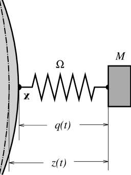
Figure 1: Schematic diagram of the coupling model between a solid sphere and a resonator. The notation is that in the text, but sub-indices have been dropped for clarity. The dashed-dotted arc line on the left indicates the position of the undeformed sphere’s surface, and the solid arc its actual position.

I shall assume that the resonators only move radially, and also that Classical Elasticity theory [ll70] is sufficiently accurate for the present purposes. In these circumstances we thus have

$$\halign to=0.0pt{\@eqnsel\hskip\@centering$\displaystyle{#}$&\global\@eqcnt\@ne\hskip 2\arraycolsep\hfil${#}$\hfil&\global\@eqcnt\tw@\hskip 2\arraycolsep$\displaystyle{#}$\hfil&\llap{#}\cr 0.0pt plus 1000.0pt$\displaystyle{ \varrho\,\frac{\partial^{2} {\bf u}}{\partial t^{2}} &10.0pt\hfil${= &10.0pt$\displaystyle{\mu\nabla^{2} {\bf u} + (\lambda+\mu)\,\nabla(\nabla{\bf\cdot}{\bf u}) + {\bf f}({\bf x},t) {}&\hbox to0.0pt{\hss($82\mathrm{.a}$)\cr\penalty 10000\vskip 3.0pt\vskip 6.99997pt\cr 0.0pt plus 1000.0pt$\displaystyle{\ddot{z}_{a}(t) &10.0pt\hfil${= &10.0pt$\displaystyle{-\Omega_{a}^{2}\, \left[z_{a}(t)-u_{a}(t)\right]+\xi_{a}^{\rm external}(t)\ , \qquad a=1,\ldots,J &\hbox to0.0pt{\hss($82\mathrm{.b}$)\cr}}}}}}}}}$$

where ${\bf n}_{a}\/$ $\equiv$ ${\bf x}_{a}/R\/$ is the outward pointing normal at the the $a\/$-th resonator’s attachment point, and

$$u_{a}(t)\equiv{\bf n}_{a}\!\cdot\!{\bf u}({\bf x}_{a},t)\ ,\qquad a=1,\ldots,J$$ (83)

is the radial deformation of the sphere’s surface at ${\bf x}_{a}\/$. A dot ( $\dot{}$ ) is an abbreviation for time derivative. The term in square brackets in (2) is thus the spring deformation —$q(t)$ in Figure 1.

${\bf f}({\bf x},t)$ in the rhs of (2) contains the density of all non-internal forces acting on the sphere, which is expediently split into a component due the resonators’ back action and an external action proper, which can be a GW signal, a calibration signal, etc. Then

$${\bf f}({\bf x},t)={\bf f}_{\rm resonators}({\bf x},t)+{\bf f}_{\rm external}({\bf x},t)$$ (84)

Finally, $\xi_{a}^{\rm external}(t)$ in the rhs of (2) is the force per unit mass (acceleration) acting on the $a\/$-th resonator due to external agents.

Given the hypothesis that the resonators are point masses, the following holds:

$${\bf f}_{\rm resonators}({\bf x},t)=\sum_{a=1}^{J}M_{a}\Omega_{a}^{2}\,\left[\,z_{a}(t)-u_{a}(t)\right]\,\delta^{(3)}({\bf x}-{\bf x}_{a})\,{\bf n}_{a}$$ (85)

where $\delta^{(3)}\/$ is the three dimensional Dirac density function.

The external forces I shall be considering in this paper will be gravitational wave signals, and also a simple calibration signal, a perpendicular hammer stroke. GW driving terms, c.f. equation (81), can be written

$${\bf f}_{\rm GW}({\bf x},t)={\bf f}^{(00)}({\bf x})\,g^{(00)}(t)\ +\ \sum_{m=-2}^{2}\,{\bf f}^{(2m)}({\bf x})\,g^{(2m)}(t)$$ (86)

for a general metric wave —see [lobo] for explicit formulas and technical details. While the spatial coefficients ${\bf f}^{(lm)}({\bf x})$ are pure form factors associated to the tidal character of a GW excitation, it is the time dependent factors $g^{(lm)}(t)$ which carry the specific information on the incoming GW. The purpose of a GW detector is to determine the latter coefficients on the basis of suitable measurements.

If a GW sweeps the observatory then the resonators themselves will also be affected, of course. They will be driven, relative to the sphere’s centre, by a tidal acceleration which, since they only move radially, is given by

$$\xi_{a}^{\rm GW}(t)=c^{2}\,R_{0i0j}(t)\,x_{a,i}n_{a,j}\ ,\qquad a=1,\ldots,J$$ (87)

where $R_{0i0j}(t)$ are the “electric” components of the GW Riemann tensor at the centre of the sphere. These can be easily manipulated to give

$$\xi_{a}^{\rm GW}(t)=R\,\sum_{\stackrel{{\scriptstyle\scriptstyle l=0\ {\rm and}\ 2}}{{m=-l,...,l}}}\,Y_{lm}({\bf n}_{a})\,g^{(lm)}(t)\ ,\qquad a=1,\ldots,J$$ (88)

where $R\/$ is the sphere’s radius.

I shall also be later considering the response of the system to a particular calibration signal, consisting in a hammer stroke with intensity ${\bf f}_{0}$, delivered perpendicularly to the sphere’s surface at point ${\bf x}_{0}$:

$${\bf f}_{\rm stroke}({\bf x},t)={\bf f}_{0}\,\delta^{(3)}({\bf x}-{\bf x}_{0})\,\delta(t)$$ (89)

which is modeled as an impulsive force in both space and time variables. Unlike GW tides, a hammer stroke will be applied on the sphere’s surface, so it has no direct effect on the resonators. In other words,

$$\xi_{a}^{\rm stroke}(t)=0\ ,\qquad a=1,\ldots,J$$ (90)

The fundamental equations thus finally read:

$$ ϱ∂2u∂t2= (91.a)& ∑_b=1^J M_bΩ_b^2 [z_b(t)-u_b(t)]δ^(3)(x-x_b) n_b + f_external(x,t) (91.bz¨_a(t) = -Ω_a^2 [z_a(t)-u_a(t)]+ ξ_a^external(t) ,   a=1,…,J (91.c)  where 𝐟external(𝐱,t) will be given by either (86) or (89), as the case may be. Likewise, ξaexternal(t) will be given by (88) or (90), respectively. The remainder of this paper will be concerned with finding solutions to the system of coupled differential equations (2), and with their meaning and consequences.  3 Green function formalism In order to solve equations (2) I shall resort to Green function formalism. The essentials of this procedure in the context of the present problem can be found in detail in reference [lobo]; more specific technicalities are given in appendix LABEL:app:a. By means of such formalism equations (2) become the following integro-differential system: ua(t) = uaexternal(t) + ∑b=1Jηb∫0tKab(t-t’) [zb(t’)-ub(t’)]dt’ (92.a)¨za(t) = ξaexternal(t) -Ωa2[za(t)-ua(t)],   a=1,…,J (92.b)whereu_a^external(t) ≡ n_a​⋅​u^external(x_a,t),andu^external(x,t)isthebare(i.e.,withoutattachedresonators)sphere′sresponsetotheexternalforcesf_external(x,t)intherhsof(2).K_ab(t)isakernelmatrixdefinedbythefollowingweightedsumofdiadicproductsofwavefunctions: Kab(t)=Ωb2∑NωN-1[nb​⋅​uN∗(xb)][na​⋅​uN(xa)]sinωNt (93) Finally,themassratiosoftheresonatorstotheentirespherearedefinedby ηb≡MbM,b=1,…,J (94) andwillbesmallparametersinarealdevice.Beforeproceedingfurther,letusbrieflypauseforaqualitativeinspectionofequations(3).Equation(3)showsthatthesphere′ssurfacedeformationsu_a(t)aremadeupoftwocontributions:oneduetotheactionofexternalagents(GWsorother),containedinu_a^external(t),andanotheroneduetocouplingtotheresonators.Thelatteriscommandedbythesmallparametersη_b,andcorrelatestoallofthesphere′sspheroidaleigenmodesthroughthekernelmatrixK_ab(t).ThishasconsequencesforGWdetectors,foreventhoughGWsmayonlycoupletoquadrupoleandmonopolespheroidalmodesofthefreesphere[lobo, bian],attachmentofresonatorscauses,aswesee,couplingbetweentheseandtheothermodesoftheantenna;conversely,thelatterback-actontheformer,too.AsIshallshortlyprove,suchundesirableeffectscanbeminimisedbysuitablytuningtheresonators′frequencies. 3.1 Laplace transform domain equations A solution to equations (3) will now be attempted. Equation (3) is an integral equation belonging in the general class of Volterra equations [tricomi], but the usual iterative solution to it by repeated substitution of ub(t) into the kernel integral is not viable here due to the dynamical contribution of zb(t), which is in turn governed by the differential equation (3). A better suited method to solve this integro-differential system is to Laplace-transform it. I denote the Laplace transform of a generic function of time f(t) with a caret ( ^ ) on its symbol, e.g., ^f(s)≡∫0∞f(t)e-stdt (95) and make the assumption that the system is at rest before an instant of time, t = 0, say, or u(x,0)=˙u(x,0)=za(0)=˙za(0)=0 (96) Equations (3) then adopt the equivalent form ^ua(s) = ^uaexternal(s)-∑b=1Jηb^Kab(s)[^zb(s)-^ub(s)] (97.a) s2^za(s) = ^ξaexternal(s)-Ωa2[^za(s)-^ua(s)],a=1,…,J (97.b) for which use has been made of the convolution theorem for Laplace transforms. A further simplification is accomplished if we consider that we shall in practice be only concerned with the measurable quantities qa(t)≡za(t)-ua(t),a=1,…,J (98) representing the resonators’ actual elastic deformations —cf. Figure 1. It is readily seen that these verify the following: ∑b=1J[δab+ηbs2s2+Ωa2^Kab(s)]^qb(s)=-s2s2+Ωa2^uaexternal(s)+^ξaexternal(s)s2+Ωa2,a=1,…,J (99) Equations (99) constitute a significant simplification of the original problem, as they are a set of just J algebraic rather than integral or differential equations. We must solve them for the unknowns ^qa(s), then perform inverse Laplace transforms to revert to qa(t). I come to this next. 4 System response to a Gravitational Wave Our concern now is the actual system response when it is acted upon by an incoming GW. It will be calculated by making a number of simplifying assumptions, more precisely: The detector is perfectly spherical. The resonators have identical masses and resonance frequencies. The resonators’ frequency is accurately matched to one of the sphere’s oscillation eigenfrequencies. It will be shown below (section LABEL:sec:symdef) that a real system can be appropriately treated as one which deviates by definite amounts from this idealised construct. Therefore detailed knowledge of the ideal system behaviour is essential for all purposes: such is the justification for the above simplifications. The wave-functions unlm(x) of an elastic sphere can be found in reference [lobo] in full detail, and I shall keep the notation of that paper for them. The Laplace transform of the kernel matrix (93) can thus be expressed as —see equation (LABEL:A3.20) in appendix LABEL:app:a: ^Kab(s)=∑nlΩb2s2+ωnl2|Anl(R)|22l+14πPl(na​⋅​nb)≡∑nlΩb2s2+ωnl2χab(nl) (100) where the last term simply defines the quantities χab(nl). Note that the sums here extend over the entire spectrum of the solid sphere. The assumption that all the resonators are identical simply means that η1=…=ηJ≡η,Ω1=…=ΩJ≡Ω (101) The third hypothesis makes reference to the fundamental idea behind using resonators, which is to have them tuned to one of the frequencies of the sphere’s spectrum. This is expressed by Ω=ωn0l0 (102) where ωn0l0 is a specific and fixed frequency of the spheroidal spectrum. In a GW detector it will only make sense to choose l0 = 0 or l0 = 2, as only monopole and quadrupole sphere modes couple to the incoming signal; in practice, n0 will refer to the first, or perhaps second harmonic [clo]. I shall however keep the generic expression (102) for the time being in order to encompass all the possibilities with a unified notation. Based on the above hypotheses, equation (99) can be rewritten in the form ∑b=1J[δab+η∑nlΩ2s2(s2+Ω2)(s2+ωnl2)χab(nl)]^qb(s)=-s2s2+Ω2^uaGW(s)+^ξaGW(s)s2+Ω2,(Ω=ωn0l0) (103) where ^ξaGW(s) is the Laplace transform of (88), i.e., ^ξaGW(s)=R∑m=-l,…,ll=0and 2Ylm(na)^g(lm)(s),a=1,…,J (104) As mentioned at the end of the previous section, the matrix in the lhs of (103) must now be inverted; this will give us an expression for ^qa(s), whose inverse Laplace transform will take us back to the time domain. A simple glance at the equation suffices however to grasp the unsurmountable difficulties of accomplishing this analytically. Thankfully, though, a perturbative approach is applicable when the masses of the resonators are small compared to the mass of the whole sphere, i.e., when the inequality η≪1 (105) holds. I shall henceforth assume that this is the case, as also is with cylindrical bar resonant transducers. It is shown in appendix LABEL:app:b that the perturbative series happens in ascending powers of η1/2, rather than η itself, and that the lowest order contribution has the form ^qa(s)=η-1/2∑l,m^Λa(lm)(s;Ω)^g(lm)(s)+O(0),a=1,…,J (106) where O(0) stands for terms of order η0 or smaller. Here, ^Λa(lm)(s;Ω) is a transfer function matrix which relates linearly the system response ^qa(s) to the GW amplitudes ^g(lm)(s), in the usual sense that qa(t) is given by the convolution product of the signal g(lm)(t) with the time domain expression, Λa(lm)(t;Ω), of ^Λa(lm)(s;Ω). The detector is thus seen to act as a linear filter on the GW signal, whose frequency response is characterised by the properties of ^Λa(lm)(s;Ω). More specifically, the filter has a number of characteristic frequencies which correspond to the imaginary parts of the poles of ^Λa(lm)(s;Ω). As also shown in appendix LABEL:app:b, these frequencies are the symmetric pairs ωa±2=Ω2(1±2l+14π|An0l0(R)|ζaη1/2)+O(η),a=1,…,J (107) where ζa2 is the a-th eigenvalue of the Legendre matrix Pl0(na​⋅​nb),a,b=1,…,J (108) associated to the multipole (l0) selected for tuning —see (102). These frequency pairs correspond to beats, typical of resonantly coupled oscillating systems —we shall find them again in section LABEL:sec:hs in a particularly illuminating example. Equation (106) neatly displays the amplification coefficient η-1/2 of the resonators’ motion amplitudes, which corresponds to the familiar resonant energy transfer in coupled systems of linear oscillators [as93]. The specific form of the transfer function matrix ^Λa(lm)(s;Ω) depends both on the selected mode to tune the resonator frequency Ω and on the resonator distribution geometry. I now come to a discussion of these. 4.1 Monopole gravitational radiation sensing General Relativity, as is well known, forbids monopole GW radiation. More general metric theories, e.g. Brans-Dicke [bd61], do however predict this kind of radiation. It appears that a spherical antenna is potentially sensitive to monopole waves, so it can serve the purpose of thresholding, or eventually detecting them. It is therefore relevant to consider the system response to scalar waves. This clearly requires that the resonator set be tuned to a monopole harmonic of the sphere, i.e., Ω=ωn0,(l0=0) (109) where n tags the chosen harmonic —most likely the first (n = 1) in a thinkable device. Since P0(z) ≡ 1 (for all z) the eigenvalues of P0(na​⋅​nb) are, clearly, ζ12=J,ζ22=…=ζJ2=0 (110) for any resonator distribution. The tuned mode frequency thus splits into a single strongly coupled pair: ω±2=Ω2(1±J4π|An0(R)|η1/2)+O(η),Ω=ωn0 (111) The Λ-matrix of equation (106) is seen to be in this case ^Λa(lm)(s;ωn0)=(-1)Jan0J12[(s2+ω+2)-1-(s2+ω-2)-1]δl0δm0 (112) whence the system response is ^qa(s)=η-1/2(-1)JJan012[(s2+ω+2)-1-(s2+ω-2)-1]^g(00)(s)+O(0),a=1,…,J (113) regardless of resonator positions. The overlap coefficient an0 is given by (3), and can be calculated by means of numerical computer programmes. By way of example, a10/R = 0.214, and a20/R = -0.038 for the first two harmonics. A few interesting facts are displayed by equation (113). First, as already stressed, it is seen that if the resonators are tuned to a monopole detector frequency then only monopole wave amplitudes couple strongly to the system, even if quadrupole radiation amplitudes are significantly high at the observation frequencies ω±. Also, the amplitudes ^qa(s) are equal for all a, as corresponds to the spherical symmetry of monopole sphere’s oscillations, and are proportional to J-1/2, a factor we should indeed expect as an indication that GW energy is evenly distributed amongst all the resonators. A single transducer suffices to experimentally determine the only monopole GW amplitude ^g(00)(s), of course, but (113) provides the system response if more than one sensor is mounted on the antenna for whatever reasons. 4.2 Quadrupole gravitational radiation sensing I now consider the more interesting case of quadrupole motion sensing. The choice is now, clearly, Ω=ωn2,(l0=2) (114) where n labels the chosen harmonic —most likely the first (n = 1) or the second (n = 2) in a practical system. The evaluation of the Λ-matrix is now considerably more involved [serrano], yet a remarkably elegant form is found for it: ^Λa(lm)(s;ωn2)=(-1)N4π5an2∑b=1J{∑ζc≠012[(s2+ωc+2)-1-(s2+ωc-2)-1]va(c)vb(c)∗ζc}Y2m(nb)δl2 (115) where va(c) is the c-th normalised eigenvector of P2(na​⋅​nb), associated to the non-null eigenvalue ζc2. Let me stress that equation (115) explicitly shows that at most 5 pairs of modes, of frequencies ωc±, couple strongly to quadrupole GW amplitudes, no matter how many resonators in excess of 5 are mounted on the sphere. The tidal overlap coefficients a2n can also be calculated using (3), and give for the first two harmonics a12R=0.328,a22R=0.106 (116) The system response is thus ^qa(s) = η-1/2(-1)J4π5an2∑b=1J{∑ζc≠012[(s2+ωc+2)-1-(s2+ωc-2)-1]va(c)vb(c)∗ζc}× (117) ×∑m=-22Y2m(nb)^g(2m)(s)+O(0),a=1…,J Equation (117) is completely general, i.e., it is valid for any resonator configuration over the sphere’s surface, and for any number of resonators. It describes precisely how all 5 GW amplitudes ^g(2m)(s) interact with all 5 strongly coupled system modes; like before, only quadrupole wave amplitudes are seen in the detector (to leading order) when Ω = ωn2, even if the incoming wave carries significant monopole energy at the frequencies ωc±. The degree of generality and algebraic simplicity of (117) is new in the literature. As we shall now see, it makes possible a systematic search for different resonator distributions and their properties. fragmentsfragments ϱfragments∂2ufragments∂t2= (91.a)& ∑_b=1^J M_bΩ_b^2 [z_b(t)-u_b(t)]δ^(3)(x-x_b) n_b + f_external(x,t) (91.b¨z_a(t) = -Ω_a^2 [z_a(t)-u_a(t)]+ ξ_a^external(t) ,   a=1,…,J (91.c)  where fexternal(x,t) will be given by either (86) or (89), as the case may be. Likewise, ξ𝑎external(t) will be given by (88) or (90), respectively. The remainder of this paper will be concerned with finding solutions to the system of coupled differential equations (2), and with their meaning and consequences.  3 Green function formalism In order to solve equations (2) I shall resort to Green function formalism. The essentials of this procedure in the context of the present problem can be found in detail in reference [lobo]; more specific technicalities are given in appendix LABEL:app:a. By means of such formalism equations (2) become the following integro-differential system: ua(t) = uaexternal(t) + ∑b=1Jηb∫0tKab(t-t’) [zb(t’)-ub(t’)]dt’ (92.a)¨za(t) = ξaexternal(t) -Ωa2[za(t)-ua(t)],   a=1,…,J (92.b)whereu_a^external(t) ≡ n_a​⋅​u^external(x_a,t),andu^external(x,t)isthebare(i.e.,withoutattachedresonators)sphere′sresponsetotheexternalforcesf_external(x,t)intherhsof(2).K_ab(t)isakernelmatrixdefinedbythefollowingweightedsumofdiadicproductsofwavefunctions: Kab(t)=Ωb2∑NωN-1[nb​⋅​uN∗(xb)][na​⋅​uN(xa)]sinωNt (93) Finally,themassratiosoftheresonatorstotheentirespherearedefinedby ηb≡MbM,b=1,…,J (94) andwillbesmallparametersinarealdevice.Beforeproceedingfurther,letusbrieflypauseforaqualitativeinspectionofequations(3).Equation(3)showsthatthesphere′ssurfacedeformationsu_a(t)aremadeupoftwocontributions:oneduetotheactionofexternalagents(GWsorother),containedinu_a^external(t),andanotheroneduetocouplingtotheresonators.Thelatteriscommandedbythesmallparametersη_b,andcorrelatestoallofthesphere′sspheroidaleigenmodesthroughthekernelmatrixK_ab(t).ThishasconsequencesforGWdetectors,foreventhoughGWsmayonlycoupletoquadrupoleandmonopolespheroidalmodesofthefreesphere[lobo, bian],attachmentofresonatorscauses,aswesee,couplingbetweentheseandtheothermodesoftheantenna;conversely,thelatterback-actontheformer,too.AsIshallshortlyprove,suchundesirableeffectscanbeminimisedbysuitablytuningtheresonators′frequencies. 3.1 Laplace transform domain equations A solution to equations (3) will now be attempted. Equation (3) is an integral equation belonging in the general class of Volterra equations [tricomi], but the usual iterative solution to it by repeated substitution of ub(t) into the kernel integral is not viable here due to the dynamical contribution of zb(t), which is in turn governed by the differential equation (3). A better suited method to solve this integro-differential system is to Laplace-transform it. I denote the Laplace transform of a generic function of time f(t) with a caret ( ^ ) on its symbol, e.g., ^f(s)≡∫0∞f(t)e-stdt (95) and make the assumption that the system is at rest before an instant of time, t = 0, say, or u(x,0)=˙u(x,0)=za(0)=˙za(0)=0 (96) Equations (3) then adopt the equivalent form ^ua(s) = ^uaexternal(s)-∑b=1Jηb^Kab(s)[^zb(s)-^ub(s)] (97.a) s2^za(s) = ^ξaexternal(s)-Ωa2[^za(s)-^ua(s)],a=1,…,J (97.b) for which use has been made of the convolution theorem for Laplace transforms. A further simplification is accomplished if we consider that we shall in practice be only concerned with the measurable quantities qa(t)≡za(t)-ua(t),a=1,…,J (98) representing the resonators’ actual elastic deformations —cf. Figure 1. It is readily seen that these verify the following: ∑b=1J[δab+ηbs2s2+Ωa2^Kab(s)]^qb(s)=-s2s2+Ωa2^uaexternal(s)+^ξaexternal(s)s2+Ωa2,a=1,…,J (99) Equations (99) constitute a significant simplification of the original problem, as they are a set of just J algebraic rather than integral or differential equations. We must solve them for the unknowns ^qa(s), then perform inverse Laplace transforms to revert to qa(t). I come to this next. 4 System response to a Gravitational Wave Our concern now is the actual system response when it is acted upon by an incoming GW. It will be calculated by making a number of simplifying assumptions, more precisely: The detector is perfectly spherical. The resonators have identical masses and resonance frequencies. The resonators’ frequency is accurately matched to one of the sphere’s oscillation eigenfrequencies. It will be shown below (section LABEL:sec:symdef) that a real system can be appropriately treated as one which deviates by definite amounts from this idealised construct. Therefore detailed knowledge of the ideal system behaviour is essential for all purposes: such is the justification for the above simplifications. The wave-functions unlm(x) of an elastic sphere can be found in reference [lobo] in full detail, and I shall keep the notation of that paper for them. The Laplace transform of the kernel matrix (93) can thus be expressed as —see equation (LABEL:A3.20) in appendix LABEL:app:a: ^Kab(s)=∑nlΩb2s2+ωnl2|Anl(R)|22l+14πPl(na​⋅​nb)≡∑nlΩb2s2+ωnl2χab(nl) (100) where the last term simply defines the quantities χab(nl). Note that the sums here extend over the entire spectrum of the solid sphere. The assumption that all the resonators are identical simply means that η1=…=ηJ≡η,Ω1=…=ΩJ≡Ω (101) The third hypothesis makes reference to the fundamental idea behind using resonators, which is to have them tuned to one of the frequencies of the sphere’s spectrum. This is expressed by Ω=ωn0l0 (102) where ωn0l0 is a specific and fixed frequency of the spheroidal spectrum. In a GW detector it will only make sense to choose l0 = 0 or l0 = 2, as only monopole and quadrupole sphere modes couple to the incoming signal; in practice, n0 will refer to the first, or perhaps second harmonic [clo]. I shall however keep the generic expression (102) for the time being in order to encompass all the possibilities with a unified notation. Based on the above hypotheses, equation (99) can be rewritten in the form ∑b=1J[δab+η∑nlΩ2s2(s2+Ω2)(s2+ωnl2)χab(nl)]^qb(s)=-s2s2+Ω2^uaGW(s)+^ξaGW(s)s2+Ω2,(Ω=ωn0l0) (103) where ^ξaGW(s) is the Laplace transform of (88), i.e., ^ξaGW(s)=R∑m=-l,…,ll=0and 2Ylm(na)^g(lm)(s),a=1,…,J (104) As mentioned at the end of the previous section, the matrix in the lhs of (103) must now be inverted; this will give us an expression for ^qa(s), whose inverse Laplace transform will take us back to the time domain. A simple glance at the equation suffices however to grasp the unsurmountable difficulties of accomplishing this analytically. Thankfully, though, a perturbative approach is applicable when the masses of the resonators are small compared to the mass of the whole sphere, i.e., when the inequality η≪1 (105) holds. I shall henceforth assume that this is the case, as also is with cylindrical bar resonant transducers. It is shown in appendix LABEL:app:b that the perturbative series happens in ascending powers of η1/2, rather than η itself, and that the lowest order contribution has the form ^qa(s)=η-1/2∑l,m^Λa(lm)(s;Ω)^g(lm)(s)+O(0),a=1,…,J (106) where O(0) stands for terms of order η0 or smaller. Here, ^Λa(lm)(s;Ω) is a transfer function matrix which relates linearly the system response ^qa(s) to the GW amplitudes ^g(lm)(s), in the usual sense that qa(t) is given by the convolution product of the signal g(lm)(t) with the time domain expression, Λa(lm)(t;Ω), of ^Λa(lm)(s;Ω). The detector is thus seen to act as a linear filter on the GW signal, whose frequency response is characterised by the properties of ^Λa(lm)(s;Ω). More specifically, the filter has a number of characteristic frequencies which correspond to the imaginary parts of the poles of ^Λa(lm)(s;Ω). As also shown in appendix LABEL:app:b, these frequencies are the symmetric pairs ωa±2=Ω2(1±2l+14π|An0l0(R)|ζaη1/2)+O(η),a=1,…,J (107) where ζa2 is the a-th eigenvalue of the Legendre matrix Pl0(na​⋅​nb),a,b=1,…,J (108) associated to the multipole (l0) selected for tuning —see (102). These frequency pairs correspond to beats, typical of resonantly coupled oscillating systems —we shall find them again in section LABEL:sec:hs in a particularly illuminating example. Equation (106) neatly displays the amplification coefficient η-1/2 of the resonators’ motion amplitudes, which corresponds to the familiar resonant energy transfer in coupled systems of linear oscillators [as93]. The specific form of the transfer function matrix ^Λa(lm)(s;Ω) depends both on the selected mode to tune the resonator frequency Ω and on the resonator distribution geometry. I now come to a discussion of these. 4.1 Monopole gravitational radiation sensing General Relativity, as is well known, forbids monopole GW radiation. More general metric theories, e.g. Brans-Dicke [bd61], do however predict this kind of radiation. It appears that a spherical antenna is potentially sensitive to monopole waves, so it can serve the purpose of thresholding, or eventually detecting them. It is therefore relevant to consider the system response to scalar waves. This clearly requires that the resonator set be tuned to a monopole harmonic of the sphere, i.e., Ω=ωn0,(l0=0) (109) where n tags the chosen harmonic —most likely the first (n = 1) in a thinkable device. Since P0(z) ≡ 1 (for all z) the eigenvalues of P0(na​⋅​nb) are, clearly, ζ12=J,ζ22=…=ζJ2=0 (110) for any resonator distribution. The tuned mode frequency thus splits into a single strongly coupled pair: ω±2=Ω2(1±J4π|An0(R)|η1/2)+O(η),Ω=ωn0 (111) The Λ-matrix of equation (106) is seen to be in this case ^Λa(lm)(s;ωn0)=(-1)Jan0J12[(s2+ω+2)-1-(s2+ω-2)-1]δl0δm0 (112) whence the system response is ^qa(s)=η-1/2(-1)JJan012[(s2+ω+2)-1-(s2+ω-2)-1]^g(00)(s)+O(0),a=1,…,J (113) regardless of resonator positions. The overlap coefficient an0 is given by (3), and can be calculated by means of numerical computer programmes. By way of example, a10/R = 0.214, and a20/R = -0.038 for the first two harmonics. A few interesting facts are displayed by equation (113). First, as already stressed, it is seen that if the resonators are tuned to a monopole detector frequency then only monopole wave amplitudes couple strongly to the system, even if quadrupole radiation amplitudes are significantly high at the observation frequencies ω±. Also, the amplitudes ^qa(s) are equal for all a, as corresponds to the spherical symmetry of monopole sphere’s oscillations, and are proportional to J-1/2, a factor we should indeed expect as an indication that GW energy is evenly distributed amongst all the resonators. A single transducer suffices to experimentally determine the only monopole GW amplitude ^g(00)(s), of course, but (113) provides the system response if more than one sensor is mounted on the antenna for whatever reasons. 4.2 Quadrupole gravitational radiation sensing I now consider the more interesting case of quadrupole motion sensing. The choice is now, clearly, Ω=ωn2,(l0=2) (114) where n labels the chosen harmonic —most likely the first (n = 1) or the second (n = 2) in a practical system. The evaluation of the Λ-matrix is now considerably more involved [serrano], yet a remarkably elegant form is found for it: ^Λa(lm)(s;ωn2)=(-1)N4π5an2∑b=1J{∑ζc≠012[(s2+ωc+2)-1-(s2+ωc-2)-1]va(c)vb(c)∗ζc}Y2m(nb)δl2 (115) where va(c) is the c-th normalised eigenvector of P2(na​⋅​nb), associated to the non-null eigenvalue ζc2. Let me stress that equation (115) explicitly shows that at most 5 pairs of modes, of frequencies ωc±, couple strongly to quadrupole GW amplitudes, no matter how many resonators in excess of 5 are mounted on the sphere. The tidal overlap coefficients a2n can also be calculated using (3), and give for the first two harmonics a12R=0.328,a22R=0.106 (116) The system response is thus ^qa(s) = η-1/2(-1)J4π5an2∑b=1J{∑ζc≠012[(s2+ωc+2)-1-(s2+ωc-2)-1]va(c)vb(c)∗ζc}× (117) ×∑m=-22Y2m(nb)^g(2m)(s)+O(0),a=1…,J Equation (117) is completely general, i.e., it is valid for any resonator configuration over the sphere’s surface, and for any number of resonators. It describes precisely how all 5 GW amplitudes ^g(2m)(s) interact with all 5 strongly coupled system modes; like before, only quadrupole wave amplitudes are seen in the detector (to leading order) when Ω = ωn2, even if the incoming wave carries significant monopole energy at the frequencies ωc±. The degree of generality and algebraic simplicity of (117) is new in the literature. As we shall now see, it makes possible a systematic search for different resonator distributions and their properties. $$