Suspensions Thermal Noise in the LIGO Gravitational Wave Detector

Abstract

We present a calculation of the maximum sensitivity achievable by the LIGO Gravitational wave detector in construction, due to limiting thermal noise of its suspensions. We present a method to calculate thermal noise that allows the prediction of the suspension thermal noise in all its 6 degrees of freedom, from the energy dissipation due to the elasticity of the suspension wires. We show how this approach encompasses and explains previous ways to approximate the thermal noise limit in gravitational waver detectors. We show how this approach can be extended to more complicated suspensions to be used in future LIGO detectors.

I Introduction

Thermal noise is a fundamental limit to the sensitivity of gravitational wave detectors, such as the ones being built in the use by the LIGO project[1]. Thermal noise is associated with sources of energy dissipation [2], following the Fluctuation-Dissipation Theorem. Thermal noise comes in at least two important kinds: one due to the brownian motion of the mirrors, associated with the losses in the mirrors’ material; and another due to the suspension of the mirrors, due to the losses in the wires’ material. The limits following from these assumptions (losses due to elastic properties of materials) are a lower limit to the noise in the detector, since there may always be other sources of energy dissipation in imperfect clamps, mirror attachments, etc. But the correct calculation of the thermal noise limit is essential to the design of detectors and diagnostics of the already-built detectors. We will deal in this article with thermal noise of suspensions (not of internal modes of the mirrors themselves), and assume only losses due to the elasticity of the suspension wires.

The calculation of thermal noise can be done in several ways [3],[4],[5],[6],[7]. All of these follow the Fluctuation-Dissipation Theorem (FDT), but a complication arises because in suspensions there are two sources of energy (gravitational and elastic), but only one of them is “lossy” (elastic energy). Moreover, the losses in the suspension wires are associated with their bending, and seems to be localized at the top and bottom of the wires. The ways to include these features into the thermal noise calculations are different enough that they have led to some confusion among the gravitational wave community. Also, attention has been paid mostly to the horizontal motion of the suspension, although all modes (angular, transverse, and vertical) appear to some degree into the detector’s noise. We present a method to calculate thermal noise that allows the prediction of the suspension thermal noise in all its 6 degrees of freedom, from the energy dissipation due to the elasticity of the suspension wires. We also show how the contributions of thermal noise in different directions can be sensed by the interferometer through the laser beam position and direction. The results will follow from the consideration of the coupled equations of the suspension and the continuous wire, first presented in [3] for just the horizontal degree of freedom. We show how this approach encompasses and explains previous ways to approximate the thermal noise limit in gravitational wave detectors. We show how this approach can be extended to more complicated suspensions to be used in future LIGO detectors. To our knowledge, this is the first time the thermal noise of angular degrees of freedom is presented, and that all suspension degrees of freedom are calculated in an unified approach.

Since the full treatment of the problem is somewhat involved, we present first the problem without considering the elasticity of the wire, but adding a second, lossy, energy source to the gravitational energy in the treatment of the mechanical pendulum, and introduce the concepts of “dilution factors”, and “effective” quality factors. We also start with one and two-degrees of freedom suspensions instead of 6-dof. With these tools, most of the issues can be clearly presented and then we follow to the full treatment of the LIGO suspensions, presenting the implications for LIGO.

II Simple pendulum cases: dilution factors, coupled modes, effective quality factors.

The full treatment of this case, considering the elastic coupling of the wire to the suspension, was presented in [3]. Here, we will present the simpler “mechanical” treatment of this case, which will introduce the concepts of “dilution factors”, and measured vs. effective quality factors.

A A simple oscillator with a dissipative energy source

We first recapitulate the calculation of thermal noise in the simplest case, a suspended point mass. The potential energy is $PE=(1/2)Kx^{2}$ and $F_{K}=-dV/dx=-Kx$. The kinetic energy is $KE=(1/2)M\dot{x}^{2}$. The admittance to an external force $F_{ext}$ is given by

$$Y\equiv i\omega\frac{x}{F_{ext}}=i\omega\frac{1}{K-M\omega^{2}}$$

The admittance has a pole at the system eigenfrequency $w_{0}^{2}=K/M$. If $K$ is real, the resonance has an infinite amplitude and zero width. If the spring constant has an imaginary part representing an energy loss, $K\rightarrow K(1+i\phi)$, then the amplitude $|Y(\omega_{0})|$ is finite, and the peak has a width determined by the complex part of the eigenfrequency $\omega_{0}^{2}=(K/M)(1+i\phi)$. The width of the peak is characterized with a quality factor $Q=1/\phi$, and it is usually measured from the free decay time $\tau$ of the natural oscillation at the frequency $\omega_{0}$: $Q=\omega_{0}\tau/2$.

The thermal noise is proportional to the real part of the admittance, and thus to $\phi$:

$$\Re[Y]=\frac{wK\phi}{(K-M\omega^{2})^{2}+K^{2}\phi^{2}}$$

We are usually interested in frequencies well above $\omega_{0}$, since the pendulum frequency $w_{0}/2\pi$ in gravitational wave detectors is usually below 1 Hz, and the detectors have their maximum sensitivity at  100 Hz. At those frequencies, the thermal noise is

$$x^{2}(\omega)=\frac{4k_{B}T_{0}}{\omega^{2}}\Re[Y]\sim\frac{4k_{B}T_{0}\omega_{0}^{2}\phi}{M\omega^{5}}$$ (1)

This how we see that the measured decay of the pendulum mode can be used to predict the suspension thermal noise at gravitational wave frequencies. Some beautiful examples of these difficult measurements and their use for gravitational wave detectors are presented in [8], for example.

B A pendulum with two energy sources: the dilution factor.

Next, we consider a suspended point mass, but we now assume there two sources of energy, gravitational and elastic, each with its own spring constant. The potential energy is then $V=V_{g}+V_{e}=(1/2)(K_{g}+K_{e})x^{2}$, and

$$\Re[Y]=\frac{\omega(K_{g}\phi_{g}+K_{e}\phi_{e})}{((K_{g}+K_{e})-M\omega^{2})^{2}+(K_{g}+K_{e})^{2}\phi^{2}}$$

If we assume that $K_{g}\gg K_{e}$, then

$$\Re[Y]\sim\frac{\omega(K_{g}\phi_{g}+K_{e}\phi_{e})}{(K_{g}-M\omega^{2})^{2}+K_{g}^{2}\phi^{2}}$$

and at high frequencies

$$x^{2}(\omega)=\frac{4k_{B}T_{0}}{\omega^{2}}\Re[Y]\sim\frac{4k_{B}T_{0}(K_{g}\phi_{g}+K_{e}\phi_{e})}{M^{2}\omega^{5}}$$

If $\phi_{g}=0$ (“gravity is lossless”), or at least $K_{g}\phi_{g}\ll K_{e}\phi_{e}$, then

$$\frac{4k_{B}T_{0}\omega_{0}^{2}(K_{g}/K_{e})\phi_{e}}{M\omega^{5}}$$

where $\omega_{0}^{2}\sim K_{g}/M$. We see that is the same expression as if we had just one energy source with a complex spring constant $K=K_{g}(1+i(K_{e}/K_{g})\phi_{e})$. This is why we call the factor $K_{e}/K_{g}$ the “dilution factor”: the elastic energy is the one contributing the loss factor to the otherwise loss-free $K_{g}$, but “diluted” by the small factor $K_{e}/K_{g}$. The dilution factor is also equal to the ratio of elastic energy to gravitational energy $K_{e}/K_{g}=V_{e}/V_{g}$. The concept of a dilution factor is very useful because it is usually easier to measure the loss factor $\phi_{e}$ associated with the elastic spring constant than the quality factor of the pendulum mode. This is because $K_{e}$ is usually a function of the complex Young modulus $E$, and the imaginary part of the Young modulus is easily measurable for most fiber materials, and can even be found in tables of material properties. (Of course, there are subtleties to this argument, in particular with thermoelastic or surface losses [9], but we are assuming the minimum material loss).

C A point mass suspended from an anelastic wire: calculating the dilution factor

This case is a particular case of the one treated in [3], and here we just mention it to present the approach taken to the full problem, and present some new relevant aspects.

We want to include the elasticity of the wire in the equations of motion, so we treat the suspension wire as an elastic beam, and then we have pendulum degree of freedom $x$, plus the wire’s infinite degrees of freedom $w(s)$ of transverse motion. We define a coordinate $s$, that starts at the top of the wire $s=0$, and ends at the attachment point to the mirror, $s=L$. Correspondingly, we will have an eigenfrequency, associated with the pendulum mode, and an infinite series of “violin” modes. The potential energy is $PE=(1/2)\int_{0}^{L}\rho(w^{\prime}(s))^{2}ds$, and the kinetic energy is $KE=(1/2)\int_{0}^{L}\rho(\dot{w}(s))^{2}ds+(1/2)M\dot{x}^{2}$. The solutions to the wire equation of motion, with boundary conditions $w(0)=0$ and $w(L)=x$ are $w(s)=x\sin(ks)/\sin(kL)$, and the equation of motion for the mass $M$ subject to an external force $F$ is $F=-M\omega^{2}x+Tw^{\prime}(L)=-M\omega^{2}x+(T/L)x(kL/\tan(kL))$. The admittance

$$Y=i\omega\frac{x}{F}=i\omega\frac{T}{L}\frac{\tan kL/kL}{1-\omega^{2}(ML/T)(\tan kL/kL)}$$

has a pole at the pendulum frequency $w_{p}^{2}\sim T/ML$, where $kL\ll 1$, and an infinite number of poles at the violin mode frequencies, at frequencies $w_{n}\sim(T/\rho L^{2})^{1/2}(1+(\rho L/M)n^{2}\pi^{2})$, where $kL=n\pi+\sqrt{(\rho L/M)}/(n\pi)$.

The spring “constant” associated with the wire and gravity’s restoring force $K=(T/L)(kL/\tan(kL))$ is in fact a function of frequency, although it is the usual constant $T/L$ for frequencies below the violin modes, where $kL\ll 1$. At frequencies above the first violin mode, the spring function is not even positive definite, or finite. The function $K$ is real at all frequencies because we haven’t added any source of energy loss yet. We introduce energy loss in the system by adding the wire elastic energy to the system, and then assuming a complex Young modulus. The potential energy is now $PE=(T/2)(\int_{0}^{L}w^{\prime 2}(s)ds)+(EI/2)\int_{0}^{L}w^{\prime\prime 2}(s)ds$. The equation of motion for the wire is

$$T\frac{d^{2}w(s)}{ds^{2}}-EI\frac{d^{4}w(s)}{ds^{4}}+\rho\omega^{2}w(s)=0,$$

a fourth order equation with boundary conditions $w(0)=0$, $w^{\prime}(0)=0$, and $w(L)=x$. The wire slope at the bottom, $w^{\prime}(L)$, is a free parameter (since we are assuming a point mass), and the variation of the Lagrangian with respect to $w^{\prime}(L)$ provides the fourth boundary condition for the wire: $w^{\prime\prime}(L)=0$. We can find an exact solution for the wire shape as a function of $x$, trigonometric functions of $ks$, and hyperbolic functions of $k_{e}s$, where $k,k_{e}$ are solutions to $T\kappa^{2}-EI\kappa^{4}+\rho\omega^{2}=0$ which approximate at low frequencies the perfect string wavenumber, $k^{2}\sim\rho\omega^{2}/T$ and a constant “elastic” wavenumber , $k_{e}^{2}\sim T/EI$ [3]. The distance $\Delta=\sqrt{EI/T}$ is the characteristic elastic distance over which the wire bends, especially at top and bottom clamps. In LIGO test mass suspensions, $\Delta\sim$2mm, a small fraction of $L=0.45$m. The approximations $k^{2}\sim\rho\omega^{2}/T$ and $k_{e}^{2}\sim T/EI$ are valid for frequencies that satisfy $\omega^{2}\ll T^{2}/4EI\rho$, about 12 kHz for LIGO, so we will use them in the remainder of this article. It is also equivalent to $k\Delta\ll 1$.

We also use an approximate solution for the wire shape, good to order $e^{-L/\Delta}$($\sim 10^{-99}$ (!) for LIGO):

$$w(s) = A\left(\sin(ks)-k\Delta\cos(ks)\right)$$ (3)

$$+k\Delta\left(Ae^{-s/\Delta}+Be^{-(L-s)/\Delta}\right)$$

The coefficients $A,B$ are functions of $x$ and $k$, and thus, functions of frequency:

$$A = \frac{x}{\sin(kL)-k\Delta\cos(kL)}$$

$$B = xk\Delta.$$

In the limit $\Delta\rightarrow 0$, we recover the perfect wire solution, $w(s)=x\sin(ks)/sin(kL)$. The ratio $B/A$ measures how much more (or less) the wire bends at the bottom than at the top. The elastic energy is well approximated by the contribution of the exponential terms in the wire shape, at top and bottom: $PE_{e}=(1/2)\int EI(w^{\prime\prime}(s))^{2}ds=(1/2)T\Delta^{2}\int(w^{\prime\prime}(s))^{2}ds\sim(1/2)Tk^{2}L(A^{2}+B^{2})$. At low frequencies where $kL\ll 1$, the ratio $B/A\sim\Delta/L\ll 1$, indicating that the wire bends much more at the top than at the bottom (recall this is a point mass).

The equation of motion for the mass when there is an external force $F$ is

$$F = -M\omega^{2}x+Tw^{\prime}(L)-EIw^{\prime\prime\prime}(L)$$ (4)

$$\sim -M\omega^{2}x+Tw^{\prime}(L)$$ (5)

$$\sim -M\omega^{2}x+\left(\frac{kT}{\tan kL}\frac{1+2k\Delta\tan kL}{1-(k\Delta)/(\tan kL)}\right)x$$ (6)

The ratio of the elastic force to the gravitational force, $EIw^{\prime\prime\prime}(L)/Tw^{\prime}(L)$, is of order $k\Delta\ll 1$, and thus it was dropped. If we now consider $\Delta$ complex, then the spring function

$$K=\frac{kT}{\tan kL}\frac{1+2k\Delta\tan kL}{1-(k\Delta)/(\tan kL)}$$

is also complex, and the admittance will have a non-zero real part. At frequencies below the violin modes where $kL\ll 1$, we have $K\sim(T/L)(1+\Delta/L)$, an expression that suggests a split between a real gravitational spring constant $K_{g}=T/L$ and a complex elastic spring constant $K_{e}=T\Delta/L^{2}$. However, this distinction can only be done in the approximation $\Delta/L\ll 1$, and low frequencies $kL\ll 1$. In general, however, we cannot strictly derive separate gravitational and elastic spring constants from their respective potential energy expressions: notice that the total, complex spring constant $\sim T/(L-\Delta)$ was derived from the variation of the gravitational potential energy term, which becomes complex because we use a wire shape involving the complex distance $\Delta$, satisfying the boundary conditions.

Where the approximations $\Delta/L\ll 1,\,\,kL\ll 1$ are valid, we can consider the case of two separate spring constants and thus a “dilution factor” for the pendulum loss, $K_{e}/K_{g}=\Delta/L\sim 1/232$, where the numerical value corresponds to LIGO parameters in Appendix 1. However, if we numerically calculate the exact pendulum mode quality factor, we get $1/Q_{p}=461/\phi$: this would be the measured Q from a decay time of the pendulum mode, if there are no extra losses. Did we make a “factor of 2” mistake? In fact, this factor of 2 has haunted some people in the community (including myself)[10], but there is a simple explanation. Since the elastic complex spring constant is proportional to $\Delta$, and $\Delta$ is proportional to the square root of the Young modulus, then when we make $E$ complex $E\rightarrow E(1+i\phi)$, we get $K_{e}\sim T\Delta/L^{2}\rightarrow(T\Delta/L^{2})(1+i\phi/2)$. That is, we get an extra dilution factor of two between the wire loss $\phi$ and the pendulum loss: $\phi_{p}=(K_{g}/K_{e})\Im K_{e}/\Re K_{el}=(K_{g}/K_{el})\phi/2=(\Delta/2L)\phi\sim\phi/464$, very close to the actual value. This teaches us that if the spring constant of the dissipative force is not just proportional to $E$, we will get correction factors $\partial{\log K_{e}}/\partial{\log E}$.

The thermal noise below the violin modes is well approximated by the thermal noise of a simple oscillator, as in Eqn.1, with natural eigenfrequency $w_{0}^{2}=g/L$ and loss $\phi_{0}=\Delta\phi/(2L)$. We then call $\phi_{0}=\Delta\phi/(2L)$ the “effective” loss, in this case equal to the pendulum loss (but we will see this is not always the case).

We saw that the complex spring constant $T/(\Delta-L)$was split into gravitational $T/L$ and elastic $T\Delta/L^{2}$ components. However both were derived from the gravitational force $F_{g}=-Tw^{\prime}(L)$, since the elastic force, $F_{el}=EIw^{\prime\prime\prime}(L)$, was negligible. It is because the wire shape $w(s)$ is different due to elasticity, that the function $Tw^{\prime}(L)$ is different from the pure gravitational expression $Tx/L$. The way we split gravitational and elastic contributions to the spring constant and then got a dilution factor, is only valid at low frequencies. So the argument we posed in the previous section about a dilution factor applied to the calculation in the thermal noise in the gravitational wave band is in priciple not applicable here, especially when taking into account that the total force was contributed by the variation of just the gravitational potential energy, with the elasticity in the wire shape. However, using the wire shape without low frequency approximations, we can numerically evaluate the integrals that make up the potential and elastic energies (using a real $\Delta$), and compare the ratio $V_{el}/V_{g}=\int T(w^{\prime})^{2}ds/\int EI(w^{\prime\prime})^{2}ds$ with the “low frequency” dilution factor $\Delta/L$. We show the calculation of elastic and gravitational potential energies, and their ratio, in Fig.1. At low frequencies, the ratio is constant, and equal to $\Delta/2L$: this is the dilution factor between the wire loss $\phi$ and the pendulum loss $\phi_{p}$, also the one to use for a simple-oscillator approximation of the thermal noise. It is not the ratio of the “gravitational” and “elastic” spring constants at low frequencies, but as we explained, we had no reason to expect that, since $V_{e}/V_{g}\neq K_{e}/K_{g}$. At higher frequencies, the ratio $V_{el}/V_{g}$ is not constant, and it gives correctly the dilution factors for the quality factors of the violin modes. Notice that the loss at the violin modes increases with mode number, as noted in [3]: $\phi_{n}=(\Delta/L)(1+n^{2}\pi^{2}\Delta/L)=(\Delta/L)(1+\rho L\Delta\omega_{n}^{2}/T)$, and this anharmonic behavior is well followed by the energy ratio.

In summary, the concept of dilution factor is strictly true only when the total restoring force can be split into two forces, one lossless and one dissipative, both represented with spring constants. In the general case, if we can only split the potential energy into two terms, one lossless and another dissipative, then the ratio of the energies calculated as a function of driving frequency is the exact dilution “factor”. Moreover, this ratio can be calculated as a function of frequency, and then we get the different dilution factors for all the modes in the system. This is an important lesson that also we will use more extensively in suspensions with more coupled degrees of freedom.

D A suspended extended mass: coupled degrees of freedom and observed thermal noise

We now consider an extended mass instead of a point mass, with a single generic dissipative energy source. The pendulum motion is described with the horizontal displacement of its center of mass $x$, and the pitch angle of the mass, $\theta$, as in the side view of a LIGO test mass, in Fig.7. The kinetic energy is $KE=(1/2)(M\dot{x}^{2}+J\dot{\theta}^{2})$. Instead of a spring constant, we have a 2x2 spring matrix. The potential energy is

$$PE = \frac{T}{2}(L\alpha^{2}+h\theta^{2})$$ (7)

$$= \frac{1}{2}(K_{xx}x^{2}+2K_{x\theta}x\theta+K_{\theta\theta}\theta^{2})$$ (8)

where $\alpha=(x+h\theta)/L$ and $\theta$ are the normal coordinates. The point $x+h\theta$ is the point where the wire is attached to the mirror, and the angle $\alpha$ is the angle the wire makes with the vertical. If we only consider gravitational forces, $K_{xx}=T/L,\>K_{x\theta}=Th/L$ and $K_{\theta\theta}=Th(L+h)/L$. However, we will assume that the elements of the spring matrix can be complex, and each has its own different imaginary part. The eigenfrequencies are the solutions to the equation $(K_{xx}-M\omega^{2})(K_{\theta\theta}-J\omega^{2})-K_{x\theta}^{2}=0$, or

$$2MJ\omega^{2}_{\pm}= (MK_{\theta\theta}+JK_{xx})$$ (10)

$$\pm\left((MK_{\theta\theta}-JK_{xx})^{2}+4MJK_{x\theta}^{2}\right)^{1/2}$$

In order to calculate $x^{2}(\omega)$ (the Brownian motion of the center of mass), we need to calculate the admittance $x/F$ to a horizontal force applied at the center of mass. In order to calculate $\theta^{2}(\omega)$, we need the admittance $\theta/N$ to a torque applied around the pitch axis. If the spring constants are complex, then the admittances are complex and we can calculate their real parts, and the thermal noise determined by them:

$$x^{2}(\omega)=\frac{4k_{B}T_{0}}{\omega^{2}}\Re\left[i\omega\frac{1-J\omega^{2}/K_{\theta\theta}}{K_{xx}(1-\omega^{2}/\omega_{+}^{2})(1-\omega^{2}/\omega_{-}^{2})}\right]$$

$$\theta^{2}(\omega)=\frac{4k_{B}T_{0}}{\omega^{2}}\Re\left[i\omega\frac{1-M\omega^{2}/K_{xx}}{K_{\theta\theta}(1-\omega^{2}/\omega_{+}^{2})(1-\omega^{2}/\omega_{-}^{2})}\right]$$

where the eigenfrequencies are now complex: $\omega_{\pm}^{2}\rightarrow\omega_{\pm}^{2}(1+i\phi_{\pm})$. The quality factors measurable from the free decay of each of the eigenfrequencies are $Q_{\pm}=\omega_{\pm}\tau_{\pm}/2$.

At frequencies larger than any of the eigenfrequencies, we obtain

$$x^{2}(\omega) \sim \frac{4k_{B}T_{0}}{K_{xx}\omega^{5}}((\omega_{+}^{2}\phi_{+}+\omega_{-}^{2}\phi_{-})-\phi_{\theta\theta}(K_{\theta\theta}/J))$$ (11)

$$\theta^{2}(\omega) \sim \frac{4k_{B}T_{0}}{K_{\theta\theta}\omega^{5}}((\omega_{+}^{2}\phi_{+}+\omega_{-}^{2}\phi_{-})-\phi_{xx}(K_{xx}/M))$$ (12)

The system may have the two eigenfrequencies close in value if $h(L+h)\sim J/M$ (see Fig.2), but for $h\ll J/ML$, we have $\omega_{-}^{2}\sim K_{\theta\theta}/J=Th/J$ and $\omega_{+}^{2}\sim K_{xx}/ML^{2}=T/ML$; and for $h(L+h)\gg J/M$, $\omega_{+}^{2}\sim K_{\theta\theta}/J=Th/J$ and $\omega_{-}^{2}\sim K_{xx}/ML^{2}=T/ML$. In both limits, two terms cancel in the sum of loss factors in the formulas above ($\omega_{-}^{2}\phi_{-}\sim\phi_{\theta\theta}K_{\theta\theta}/J$ for small $h$, for example) and we see that

$$x^{2}(\omega)\approx\frac{4k_{B}T_{0}\omega_{p}^{2}\phi_{xx}}{Mw^{5}}\,\,\,{\rm and}\,\,\,\theta^{2}(\omega)\approx\frac{4k_{B}T_{0}\omega_{\theta}^{2}\phi_{\theta\theta}}{J\omega^{5}}$$

Thus, even though it is a coupled system, thermal noise in $x$ is always associated mostly to $K_{xx}(1+i\phi_{xx})$ and the pendulum eigenfrequency $\omega_{p}^{2}=K_{xx}/M\sim T/ML$; and thermal noise in $\theta$ is always associated with $K_{\theta\theta}(1+i\phi_{\theta\theta})$ and the pitch eigenfrequency $\omega_{\theta}^{2}=K_{\theta\theta}/J\sim Th/J$. For both degrees of freedom $x$ and $\theta$, we obtain the thermal noise of single-dof systems. Unfortunately, neither limit (small or large $h$ with respect to $J/ML$) applies to the suspension parameters in LIGO test masses, and, more importantly, even though the approximation for the eigenfrequencies is relatively good for most values of $h$, the approximation we used for the losses is not (Fig.2). The measurable quality factors give us $\phi_{\pm}$, but we need $\phi_{xx}$ and $\phi_{\theta\theta}$ to use in the thermal noise of the pendulum, and these cannot be precisely calculated from $\phi_{\pm}$ unless we know $\phi_{x\theta}$, or a way to relate it to the other loss factors. We will do this in the next section, using the elasticity of the wire.

Notice that the forces and torques we have used to calculate the admittances $Y_{x}$ and $Y_{\theta}$, will each produce both displacement and rotation of the pendulum. This means that the thermal noise in displacement and angle are not uncorrelated. This can be exploited to find a point other than the center of mass where the laser beam in the interferometer would be sensing less displacement thermal noise than at the center of the mirror, as was done following a somewhat different logic in [5]. If we were to calculate the thermal noise at a point a distance $d$ above the center of mass, we then need to calculate the admittance of the velocity of that point ($i\omega(x+d\theta)=i\omega\chi$) to a horizontal force applied at that point. The equations of motion are

$$F= (K_{xx}-M\omega^{2})x+K_{x\theta}\theta$$

$$Fd= K_{x\theta}x+(K_{\theta\theta}-J_{y}\omega^{2})\theta$$

and then the thermal noise is

$$\chi^{2}(\omega) = \frac{4k_{B}T_{0}}{\omega^{2}}\Re\left[i\omega\frac{(x+d\theta)}{F}\right]$$ (13)

$$= \frac{4k_{B}T_{0}}{\omega^{2}}\Re\left[Y_{xx}+d^{2}Y_{\theta\theta}+2dY_{x\theta}\right]$$ (14)

$$= x^{2}(\omega)+d^{2}\theta^{2}(\omega)+2d\frac{4k_{B}T_{0}}{\omega^{2}}\Re(Y_{x\theta})$$ (15)

where $Y_{xx}$ is the admittance of $x$ to a pure force $F$, $Y_{\theta\theta}$ is the admittance of $\theta$ to a pure torque $N$, and $Y_{x\theta}$ is the admittance of a displacement $x$ to a pure torque $N$, equal to the admittance of $\theta$ to a pure force $F$. There is an optimal distance $d$ below the center of mass for which the thermal noise $\chi^{2}(\omega)$ is a minimum: this distance is $d=-\Re(Y_{x\theta})/\Re(Y_{\theta\theta})$. The resulting thermal noise is

$$\chi^{2}_{\rm min}(\omega)=x^{2}(\omega)-\frac{4k_{B}T_{0}}{\omega^{2}}\frac{(\Re Y_{x\theta})^{2}}{\Re Y_{\theta\theta}}$$

which is less than the thermal noise $x^{2}(\omega)$ observed at the center of mass. However, the expression obtained for the distance $d$ is frequency-dependent: that means we have to choose a frequency at which to optimize the sampling point.

Summarizing, we have shown that whenever there are coupled motions, the thermal noise sensed at a point whose position depends on both coordinates is not the sum in quadrature of the two thermal noise ($x^{2}$ and $d^{2}\theta^{2}(\omega)$ in our case), but a combination that depends on the “cross-admittance”. Moreover, the thermal noise of each degree of freedom cannot in general be calculated just from the measured quality factors if the modes are coupled to each other strongly enough.

E A 2-DOF pendulum suspended from a continuum wire

We add to the previous 2-DOF pendulum a continuum wire, to be able to add the losses due to the wire’s elasticity, and calculate modal and effective quality factors, as well as the point on the mirror at which we can sense the minimum thermal noise.

If we add elasticity to the problem, as in [3], the potential energy is $PE=(T/2)(\int_{0}^{L}w^{\prime 2}(s)ds+h\theta^{2})+(EI/2)\int_{0}^{L}w^{\prime\prime 2}(s)ds$. The boundary conditions for the wire equation are $w(0)=0,\,\,w(L)=x+h\theta$, and $w^{\prime}(0)=0,\,\,w^{\prime}(L)=-\theta$. The equations of motion for the pendulum are

$$-M\omega^{2}x+Tw^{\prime}(L)-EIw^{\prime\prime\prime}(L)= F$$ (16)

$$-J\omega^{2}\theta+EI(w^{\prime\prime}(L)+hw^{\prime\prime\prime}(L))= N$$ (17)

In order to complete the equations of motion of the pendulum, we need the shape of the wire at the bottom end. For this, we use the shape given by the expression in Eqn.3, but this time the top and bottom weights are given by

$$A=\frac{x+(h+\Delta)\theta}{D}$$

$$B=\frac{1}{kD}( kx(\cos(kL)+k\Delta\sin(kL))$$

$$+\theta(\sin(kL)+k(h-\Delta)\cos(kL))$$

with $D=\sin(kL)-2k\Delta\cos(kL)$ and $\Delta=\sqrt{EI/T}$ as we used earlier. With the shape known, we can write the equations for $x,\theta$ with a spring matrix:

$$(K_{xx}-M\omega^{2})x+K_{x\theta}\theta= F$$

$$K_{\theta x}x+(K_{\theta\theta}-J_{y}\omega^{2})\theta= N$$

where the spring functions are

$$K_{xx} = Tk(\cos(kL)+k\Delta\sin(kL))/D$$ (18)

$$K_{\theta\theta} = T(h+\Delta)(\sin(kL)+k(h-\Delta)\cos(kL))/D$$ (19)

$$K_{x\theta} = K_{\theta x}=Tk(h+\Delta)(\cos(kL)+k\Delta\sin(kL))/D$$ (20)

At this point, even though the expressions are complicated, we can calculate the complex admittances $Y_{xx}=i\omega x/F,\>Y_{\theta\theta}=i\omega\theta/N$ using a complex $E$ and $\Delta$. The analytical expressions for the admittances are quite involved, but we can always calculate numerically the thermal noise associated with any set of parameters. We can also calculate the widths of the peaks in the admittance, which would correspond to measurable quality factors for the pendulum, pitch, and violin modes. The plots presented in Figs. 2 and 3 were calculated using these solutions.

Fig.2 shows that the frequency and quality factor of the pendulum and pitch modes vary significantly with the pitch distance $h$. At frequencies close to the pendulum eigenfrequencies, the thermal noise spectral densities show peaks at both frequencies. However, at higher frequencies, the thermal noise $x^{2}(\omega)$ can always be approximated by the thermal noise of a simple oscilaltor as in Eqn.1, with an “effective” quality factor that fits the amplitude at high frequencies to the position of the single peak. We can similarly define an effective quality factor for the thermal noise in $\theta^{2}(\omega)$. We show in Fig.3 the actual and approximated thermal noise, with their corresponding effective quality factors found to fit best at 50 Hz. The effective quality factor at 50 Hz can be calculated as a function of pitch distance, and we show this calculation in Fig. 2. The effective pitch quality factor is well approximated, for any pitch distance, by the measurable pitch quality factor, while the pendulum effective quality factor is close to the measurable quality factor of the pendulum mode only at very small, or very large pitch distances. For the LIGO pitch distance of 8mm, the measurable pendulum quality factor is 10 times lower than the effective quality factor, and would then give a pessimistic estimate of thermal noise amplitude.

Low frequency approximation. At low frequencies, where $kL\ll 1$, we have expressions that can help us understand how the elasticity loss factor contributes to the effective quality factors, as well as to the pendulum and pitch modes. We trade this gain in simplicity for the loss of expressions valid at or above violin mode resonances.

The low frequency limit of the spring constants in Eqns. 20 is

$$K_{xx} = T/(L-2\Delta)$$

$$K_{\theta\theta} = T(h+\Delta)(L+h-\Delta)/(L-2\Delta)$$

$$K_{\theta x} = K_{x\theta}=T(h+\Delta)/(L-2\Delta).$$

If we assume $\Delta$ has an imaginary part related to the material $\phi$: $\Delta\rightarrow\Delta(1+i\phi/2)$, then we get complex spring constants. If we use these complex spring constants in Eq.10 we can calculate the loss factors of the pendulum and pitch mode, $\phi_{p}$ and $\phi_{\theta}$; and if we use them in Eqns. 12 we can get the effective quality factors. Using $h/L\ll 1$ and $\Delta/L\ll 1$, we get $Q_{{x}{\rm eff}}=1/\phi_{xx}\sim\Delta\phi/L$ and $Q_{\theta{\rm eff}}=1/\phi_{\theta\theta}\sim\Delta\phi/2(h+\Delta)$. This represents a “dilution factor” in displacement of $\Delta/L$ and in pitch of $\Delta/2(h+\Delta)$. These approximations fit very well the values shown in Fig. 2.

At low frequencies, the equations of motion for $x,\theta$ can be derived from a potential energy

$$PE_{kL\ll 1}=\frac{T}{2}\left(\frac{(x+(h+\Delta)\theta)^{2}}{L-2\Delta}+(h+\Delta)\theta^{2}\right).$$

Using a complex $\Delta$, this gives us the complex spring constants that we can use to get mode and effective quality factors. We would like to break up this potential energy into a gravitational part and an elastic part, corresponding to a real gravitational spring constant (independent of $\Delta$) and a lossy elastic spring constant. We know that if we take the limit $\Delta\rightarrow 0$ in $PE_{kL\ll 1}$, we obtain the regular potential energy $PE_{g}$ in Eq.8 for a 2 DOF pendulum without elasticity. Thus, we are tempted to say that the elastic energy is the remainder, proportional to $\Delta$, and thus having a complex spring constant when we consider a complex $\Delta$. According to this argument, we get $K_{gxx}=T/L$ and $K_{exx}=2T\Delta/L^{2}$. This would then give us a dilution factor for the displacement loss $K_{e}/K_{g}\sim 2\Delta/L$. This is the factor by which the imaginary part of $K_{el}$ is diluted; however, as explained before, we pick up another factor of two due to $K_{e}$ being proportional to $\sqrt{E}$. Thus, the dilution factor between the effective quality factor and the wire quality factor is $\Delta/L$.

Energy Ratios and the Dilution Factor.We have seen that there is another way of identifying the “gravitational” and “elastic” terms in the potential energy, using the actual potential energy expressions from which the equations of motion were derived: $PE_{g}=(T/2)(\int_{0}^{L}w^{\prime 2}(s)ds+h\theta^{2})$ and $PE_{el}=(EI/2)\int_{0}^{L}w^{\prime\prime 2}(s)ds$. For any given applied force, or torque, we can solve the equations of motion for $x,\theta$ and $w(s)$. (We don’t need to invoke a low frequency approximation to do this calculation.) Then, if we calculate the ratio of elastic to gravitational potential energy for a unit applied force, we get a function which is frequency dependent, and is equal to the dilution factors for the pitch mode at the pitch frequency, for the pendulum mode at the pendulum frequency, and for the effective quality factor at high frequencies, $\Delta/L$. We show the energy values and ratios for different values of the pitch distance in Fig. 4.

Potential Energy Densities.There is another interesting calculation we can do with the solution obtained for the wire shape, and that is to find out where in the wire the elastic potential energy is concentrated. In other words, we want to find a relationship between the variation of the dilution factor with frequency, and the curvature of the wire, mostly at the top and bottom clamps. Since both the gravitational energy and the elastic energy involve integrals over the wire length, we can define energy densities along the wire, and calculate a cumulative integral from top to bottom. The gravitational potential energy has also a term $Th\theta^{2}/2$: we define a ratio $R=Th\theta^{2}/(\int_{0}^{L}w^{\prime 2}ds)$, indicating the relative contribution of this “pitch” term. From Fig.5, we observe that the gravitational potential energy density is distributed quite homogenously along the wire, even at the first violin mode. However, the pitch term, which can be considered a “bottom” contribution, contributes most of the gravitational energy when the system is excited at the pitch eigenfrequency, but also in several other cases at the pendulum frequency and at low frequencies. The elastic energy density is concentrated at top and bottom portions of length  $2\Delta$. At low frequencies, the top contributes the most; at the pendulum eigenfrequency, the relative contributions depend strongly on $h$, but the bottom contributes at least half the energy; at the pitch eigenfrequency, the bottom contributes more than 99% of the energy; at higher frequencies, including the violin modes, top and bottom contribute equally.

Motion of points away from center of mass. We discussed previously how it was possible to find a point whose thermal noise displacement was smaller than the thermal noise displacement of the center of mass. Now that we have expressions for the complex spring functions, we can find the optimal point and discuss the differences. The cross admittance in Eq.15 is

$$Y_{x\theta} = i\omega\frac{x}{N}=i\omega\frac{\theta}{F}$$

$$= -\frac{K_{x\theta}}{(K_{xx}-M\omega^{2})(K_{\theta\theta}-J\omega^{2})}$$

$$\sim -\frac{K_{x\theta}}{MJ\omega^{4}}$$

and then the optimal point (otimized at frequencies in the gravitational wave band, above pendulum modes) is $d_{0}=-\Re(Y_{x\theta})/\Re(Y_{\theta\theta})\sim J/ML$. Notice that even though the optimal distance was deduced from the thermal noise expressions, which all involve loss factors, the optimal distance only depends on mechanical parameters. As first explained in [5], the interpretation of this distance is that when the pendulum is pushed at that point by a horizontal force, the wire doesn’t bend at the bottom clamp, producing less losses. The fact that we can recover the result from the FDT is another manifestation of the deep relationship between thermal fluctuations and energy dissipation. We show in Fig6 the dependence of the thermal noise at 50 Hz on the point probed by the laser beam on the mirror, and the ratio of the thermal noise for $d=0$ and $d=d_{0}$ at all frequencies. As expected, since the integrated rms has to be the the same for any distance at which we sense the motion, the fact that the spectral density is smaller at 50 Hz if $d=d_{0}$ means that the noise will be increased at some other frequencies: this happens mainly at frequencies below the pendulum modes.

There are many lessons to be learned from this exercise, but perhaps the most important one is that the explicit solutions to the equations of motion have many different important results:

• using the solutions to calculate the elastic and gravitational potential energies allows us to calculate a “dilution function” of frequency, equal to the dilution factor at each of the resonant modes of the system, as well as to the most important effective dilution factor at frequencies in the gravitational wave band;

• we can calculate energy densities along the wire to identify the portions of the wire most responsible for the energy loss and thus the thermal noise;

• we can use low frequency approximations to find out expressions for dilution factors that can be found using other methods, explaining in this way subtleties like factors of two;

• we can calculate the admittance of an arbitrary point in the mirror surface to the driving force, and thus find out improvements or degradation of observed noise due to beam misalignments.

III The LIGO suspensions: thermal noise of all degrees of freedom

We will now calculate the solutions to the equations of motion for the six degrees of freedom of a LIGO suspended test mass, and then use the solutions to calculate the thermal nosie of all degrees of freedom, as well as the observed tehrmal noise in the gravitational wave detector.

The mirrors at LIGO are suspended by a single wire looping around the cylindrical mass, attached at the top at a distance smaller than the mirror diameter, to provide a low yaw eigenfrequency. This is equivalent to having a mass suspended by two wires, attached slightly above the horizontal plane where the center of mass is. The mirror’s 6 degrees of freedom are the longitudinal and transverse horizontal $x$ and $y$, and the vertical $z$, displacements of the center of mass; the pitch $\theta$ and yaw $\phi$ rotations around the $y$ and $z$ axis, respectively, and the roll $\psi$ around the longitudinal $x$ axis. We show the coordinate system used and the relevant dimensions in Fig.7. The parameters used in the calculation presented are those for LIGO test mass suspensions (Large Optics Suspensions). The mass of the cylindrical mirror is 10.3 Kg, the diameter is 25cm, and the thickness 10cm. The cylindrical wires are made of steel with density $\rho=7.8\times 10^{3}{\rm kg/m^{3}}$ and 0.62mm diameter. We assumed a complex Young modulus $E=2.1\times 10^{1}1(1+10^{-3}i){\rm kg/m^{2}}$. The vertical distance between the center of mass and the top clamps is $l=45$cm, the wires are attached to the mass a distance $h=8.2$mm above the center of mass. The distance between the top attachment points is $2a=33.3$mm. (In the previous examples where one wire was used, we assumed the same wire material and the same test mirror, but we used a $0.88$mm radius, so the stress in the wires remained constant.)

Each wire element has displacement in a 2-dimensional plane transverse to the wire, ${\vec{w_{i}}}_{\perp}(s)$ and a longitudinal displacement along the wire, ${w_{i}}_{\parallel}(s)$. The kinetic energy is given by

$$KE=\frac{1}{2}( \sum_{i=1,2}\int_{0}^{L}\rho|\dot{\vec{w}_{i}}(s)|^{2}ds$$

$$+M(\dot{x}^{2}+\dot{y}^{2}+\dot{z}^{2})+J_{x}\dot{\psi}^{2}+J_{y}\dot{\theta}^{2}+J_{z}\dot{\phi}^{2})$$

The potential energy is given by the sum of the axial strain energy and the bending (transverse) strain energy in each wire:

$${PE}_{i}= \frac{1}{2}\int_{0}^{L}ds\left(T{{w_{i}}^{\prime}_{\perp}}^{2}+EA({{w_{i}^{\prime}}_{\parallel}})^{2}\right)$$

$$+\frac{1}{2}\int_{0}^{L}dsEI\left({w_{i}^{\prime\prime}}_{\perp}\right)^{2}$$

plus the energy involved in rotating the mass:

$$PE_{M}=T(h\cos\alpha(\theta^{2}+\psi^{2})-b\sin\alpha(\phi^{2}+\psi^{2})).$$

The wires will be attached at the top ($s=0$) at the coordinates $\vec{w}_{i}=(0,\pm a,l)$, where $l$ is the vertical distance of the top support from the equilibrium position of the center of mass. The wires’ transverse slopes at the top will be zero. At the bottom the wires are clamped to the mass a distance $h$ above the center of mass, and a distance $2b$ on the y-direction between the wires on each side of the mass. The angle $\alpha=\arctan((b-a)/(l-h))$ is the angle at which the wires are slanted from top to bottom when looking at the mass along the optical axis. If $b=a$, the wires hang vertically. The length of the wires is $L^{2}=(b-a)^{2}+(l-h)^{2}$. The tension in each wire is $T=Mg\cos\alpha/2$. The position of the bottom attachments when the mirror is moving with a motion described by $(x,y,z,\theta,\phi,\psi)$ are $w_{i}(L)=(x+h\theta\pm b\phi,\,y-h\psi,z\pm b\psi)$, and the slopes at the bottom are ${w^{\prime}_{i}}(L)=(-\theta,\psi,0)$.

If we express the wire transverse and longitudinal displacements in the $x,y,z$ coordinate system, we have ${w_{i}}_{\parallel}=-w_{z}\cos\alpha\pm w_{y}\sin\alpha$, and ${w_{i}}_{\perp}=\sqrt{{w_{i}}_{x}^{2}+({w_{i}}_{y}\cos\alpha\pm{w_{i}}_{z}\sin\alpha)^{2}}$ and the equations of motion become non-linear. In order to keep the problem simple, without losing any degree of freedom, we will then consider two different cases: (i) the wire only has displacements in the $x$ direction, and the mirror moves in $x,\theta,\phi$ degrees of freedom; and (ii) the wire only has displacements in the $y,z$ directions, and the mirror moves in $y,z,\psi$ degrees of freedom. We analyze these cases separately.

A Longitudinal, Pitch and Yaw Thermal Noise

The boundary conditions for the wires at the top are zero displacements and slopes, and at the bottom attachment to the mass, ${w_{\perp}}_{i}(L)=x+h\theta\pm\phi,{w^{\prime}_{\perp}}_{i}(L)=-\theta$.

We combine the wires’ transverse displacements into $w_{\pm}(s)=(w_{1}(s)\pm w_{2}(s))/2$, then the boundary conditions at the bottom are $w_{+}(L)=x-h\theta,w^{\prime}_{+}(L)=\theta,w_{-}(L)=b\phi,w^{\prime}_{-}(L)=0$. The solutions to the wire equations of motion and the boundary conditions are (up to order $e^{-L/\Delta}$) will then be $w_{\pm}(s)$ as in Eqn.3, with

$$A_{-} = \phi b/D$$

$$B_{-} = -\phi b(\cos(kL)+k\Delta\sin(kL))/D$$

$$A_{+} = (x+(h+\Delta)\theta)/D$$

$$B_{+} = -\Delta(kx(\cos(kL)+k\Delta\sin(kL))$$

$$+\theta(\sin(kL)+k(h-\Delta)\cos(kL)))/D$$

where $D=\sin(kL)-2k\Delta\cos(kL)$. The equations for the mass transverse dof subject to a force $F_{x}$ and torques $N_{y},N_{z}$, are

$$Fx = -M\omega^{2}x-2EIw_{+}^{\prime\prime\prime}(L)+2T\theta$$ (21)

$$N_{y} = -J_{y}\omega^{2}\theta+2EI\left(w_{+}^{\prime\prime}(L)+hw_{+}^{\prime\prime\prime}(L)\right)$$ (23)

$$+2Th\theta(1-\cos\alpha)$$

$$N_{z} = -J_{z}\omega^{2}\phi-2EIbw_{-}^{\prime\prime\prime}(L)-2Tb\phi\sin\alpha$$ (24)

We see that the combination $w_{+}(s)$ is associated with the $x,\theta$ degrees of freedom just as for the single wire case, while the combination $w_{-}(s)$ is associated with the yaw degree of freedom $\phi$. This is easily understood when imagining the wires moving back and forth “in phase” ($w_{-}=0$), producing displacement and pitch but nt yaw; while if they move back and forth in opposition ($w_{+}=0$), then the only effect is into mirror’s yaw. Thus, we can solve the equations for $w_{-}(s)$ and $\phi$ separately from the equations for $\omega_{+}(s),\,x$ and $\theta$: we will do so in the next parapgraphs.

Yaw angular thermal noise. The admittance of yaw $\phi$ to a torque $N_{z}$ is

$$Y_{\phi}=i\omega\frac{1}{K_{\phi}-2Tb\sin\alpha-J_{z}\omega^{2}}$$

with $K_{\phi}=(2Tb^{2}/L)(kL)(\cos(kL)+k\Delta\sin(kL))/(sin(kL)-2k\Delta\cos(kL))$. As usual, when $\Delta=\sqrt{EI/T}$ is complex, the admittance is complex and using the fluctuation-dissipation theorem we obtain $\phi^{2}(f)=(4k_{B}T_{0})\Re(Y_{\phi})/\omega^{2}$.

The effect of the tilted wires with $\alpha=(b-a)/L>0$ is to lower the restoring force, and thus the resonance frequency: in LIGO suspensions, the frequency is 0.48 Hz instead of 1.32 Hz if $b=a$. However, since $\sin\alpha\neq 0$ decreases the gravitational restoring force but not the elastic force, the dilution factor $\sim K_{e}/K_{g}$ increases, and so does the thermal noise. At frequencies where $kL\ll 1$, $K_{\phi}\sim(2Tb^{2}/L)(1+2\Delta/L)$. The thermal noise at frequencies below the violin modes, where $kL\ll 1$, is well approximated by the thermal noise of a single oscillator with resonance frequency $w_{\phi}^{2}=2Tab/JL$ and quality factor $Q_{\phi}=(L/\Delta)(a/b)(1/\phi_{w})$, where $E\rightarrow E(1+i\phi_{w})$. Thus, the “dilution factor” is $(\Delta/L)(b/a)$ (=1/72 for LIGO parameters, where $b/a=7.5$). As in the case of a simple pendulum, this dilution factor is half of the ratio of the elastic spring constant $K_{e}=(2Tb^{2}/L)(2\Delta/L)$ to the gravitational spring constant $K_{g}=2Tab/L$, because the elastic spring constant has an “extra” dilution factor of 2: if $E\rightarrow E(1+i\phi_{w})$, then $\Delta\rightarrow\Delta(1+i\phi_{w}/2)$ and $K_{e}\rightarrow K_{e}(1+i\phi_{w}/2)$. However, the ratio of elastic potential energy $\int_{0}^{L}EI(w^{\prime\prime}_{\perp})^{2}ds$ to gravitational potential energy $V_{g}=\int_{0}^{L}T(w^{\prime}_{\perp})^{2}ds-Tb\sin\alpha\,\phi^{2}$ is equal to the “right” dilution factor $(b/a)(\Delta/L)\sim 1/44$ at low frequencies, as shown in Fig. 8. The energy ratio also gives us the right dilution factor at the violin frequencies ($2\Delta/L$).

The yaw angular thermal noise may be seen in the detectors’ gravitational wave signal if the beam hits a mirror at distance $d$ to either side of the center of mass, or if it hits the mirror in a direction an angle $\gamma$ away from longitudinal. Considering both cases, the sensed thermal noise will be given by $\chi^{2}(\omega)=(d\cos\gamma+H\sin\gamma/2)^{2}\phi^{2}(\omega)$, where $H$ is the thickness of the mirror:

$$\chi^{2}(\omega) = (d\cos\gamma+(H/2)\sin\gamma)^{2}\phi^{2}(\omega)$$

$$\sim \frac{4k_{B}T}{\omega^{5}}(d\cos\gamma+(H/2)\sin\gamma)^{2}\frac{2Tb^{2}}{J_{x}L}\frac{\Delta}{L}\phi$$

where the approximation is valid between the pendulum mode and the first violin mode,  1Hz-50Hz. At 160 Hz, where the maximum sensitivity of $\sqrt{h^{2}(f)}=2.5\times 10^{-23}/\sqrt{\rm Hz}$ is expected, the yaw thermal noise is $\sqrt{\phi^{2}}(160{\rm Hz})=2.9\times 10^{-19}{\rm rad/\sqrt{Hz}}$. If the yaw thermal nose is to be kept an order of magnitude below the dominant noise source, then it is required that $d\leq$1cm and $\gamma\leq 10^{o}$.

Notice that the mirror will always be aligned normal to the laser beam to make the optical cavities resonant; however, what matters is the beam direction with respect to the coordinate system defined by the local vertical and the plane defined by the mirror in equilibrium. Presumably there will be forces applied to align the mirror, but in principle they have no effect on the response of the mirror to an oscullatory driving force such as the one we imagine in the beam’s direction, to calculate the admittance. Thus the requirement on $\gamma\leq 10^{o}$ is on the position of the mirror when there are no bias forces acting, with respect to the ultimate direction of the beam. The beam’s direction must be within  1$\mu$rad of the normal to the aligned mirror to keep the beam aligned on mirrors 4km apart, but that doesn’t mean that the mirror has not been biased by less than $10^{o}$ to get it to the final position.

Pitch and displacement thermal noise. We now solve the equations for $w_{+}(s),\theta$ and $x$. The equations for these degrees of freedom in Eqns. 24 are exactly the same as for the pendulum suspended on a single wire (Eqn. 17), except for the addition of a softening term to the torque equation, due to the tilted wires; and factors of two due to the two wires (with about half the tension) instead of a single wire. The extra term in the torque equation is a negligible contribution to the real part of $K_{\theta\theta}$, at the level of 1% for LIGO parameters. Therefore, the conclusions we obtained, with respect to the optimization of the beam location on the mirror, and the difference between effective and measurable quality factors, are equally valid here. The spring constants we obtained in Eqns. 20 involve now a factor $2T=Mg\cos\alpha$, instead of $T=Mg$ for a single wire. The elastic distance is however determined by the tension in each wire, $\Delta=\sqrt{EI/T}=\sqrt{2EI/Mg\cos\alpha}$. To keep the stress in the wires constant, the cross section area of a single supporting wire is twice the area of two each of two supporting wires. Thus, the effective quality factor determining the thermal noise for the displacement thermal noise $x^{2}(f)$ has a smaller dilution factor of $\Delta/L=1/326$, instead of 1/231 for a single wire. This is the well-know effect of reducing thermal noise by increasing the number the wires. The dilution factor for pitch is $1/14$, considerably higher than the dilution factor for yaw, $1/44$.

The displacement thermal noise at 160 Hz is $\sqrt{x^{2}(160{\rm Hz})}=1.1\times 10^{-20}{\rm m}/\sqrt{\rm Hz}$, limiting the detector sensitivity to $h=5.6\times 10^{-24}/\sqrt{\rm Hz}$. This is expected to be lower than the thermal noise due to the internal modes of the mirror mass, not considered here [11]. The pendulum thermal noise could be reduced by a factor $\sqrt{2}$, or about 40%, if the beam spot was positioned at the optimal position on the mirror. Since pendulum thermal noise is not the dominant source noise, but the detectors’ shot noise would increase due to diffraction losses, it is not advisable for LIGO to proceed this way. However, these considerations should be taken into account for future detectors, where thermal noise may be a severe limitation at low frequencies.

The pitch angular noise at 160 Hz, is $\sqrt{\theta^{2}(f)}=8.9\times 10^{-19}{\rm rad}\sqrt{\rm Hz}$. Its contribution to the sensed motion has to take into account the coupling with displacement, and we will do this in detail inthe last section.

B Vertical, transverse displacement and roll

We are now concerned with the mirror motion in its $y,z$ and $\psi$ degrees of freedom. The potential energy is $PE_{i}=(1/2)\int_{0}^{L}\left(T({w^{\prime}_{i}}_{\perp})^{2}+EI({w^{\prime\prime}_{i}}_{\perp})^{2}+EA({w^{\prime}_{i}}_{\parallel})^{2}\right)ds$ for each wire, plus $T(h\cos\alpha-b\sin\alpha)\psi^{2}$. Notice that due to the tilting of the wires, the “transverse” $w_{\perp}$ and “axial” $w_{\parallel}$ directions are not $y$ and $z$, but rotations of these directions by the wire tilt angle $\alpha$. We define ${w_{i}}_{\perp}$ for each wire pointing “out” (and thus in opposite directions if $\alpha=0$), and ${w_{i}}_{\parallel}$ pointing down along the wire, from top to bottom.

The boundary conditions at top are ${w_{i}}_{\perp}(0)=0,{w^{\prime}_{i}}_{\perp}(0)=0,{w_{i}}_{\parallel}(0)=0$, and at the bottom, ${w_{i}}_{\perp}(L)=\pm(y\cos\alpha-d\psi)+z\sin\alpha$, ${w^{\prime}_{i}}_{\perp}(L)=\pm\psi$, and ${w_{i}}_{\parallel}(L)=\pm(y\sin\alpha-c\psi)-z\cos\alpha$, where we defined two new distances $c=h\sin\alpha+b\cos\alpha$ and $d=h\cos\alpha-b\sin\alpha$. If we define as earlier, sums and differences of the two wires shape functions, $w_{\pm}(s)=(w_{1}(s)\pm w_{2}(s))/2$, then the equations of motion for the mirror degrees of freedom, when subject to external forces $F_{y},F_{z}$ and a torque $N_{x}$, are

$$F_{y} = -M\omega^{2}y+2(T{w^{\prime}_{-}}_{\perp}(L)-EI{w^{\prime\prime\prime}_{-}}_{\perp}(L))\cos\alpha$$

$$+2EA{w^{\prime}_{-}}_{\parallel}\sin\alpha$$

$$F_{z} = -M\omega^{2}z+2(T{w^{\prime}_{+}}_{\perp}(L)-EI{w^{\prime\prime\prime}_{+}}_{\perp}(L))\sin\alpha$$

$$-2EA{w^{\prime}_{+}}_{\parallel}\cos\alpha$$

$$N_{x} = -J_{x}\omega^{2}\psi-2EI(d{w^{\prime\prime\prime}_{-}}_{\perp}(L)+{w^{\prime\prime}_{-}}_{\perp}(L))$$

$$+2EAc{w^{\prime}_{-}}_{\parallel}(L)$$

The solution for the wires’ transverse motion ${w_{\pm}}_{\perp}(s)$ satisfying the boundary conditions up to order $e^{-L/\Delta}$ and $k\Delta$ are of the same form as in Eqn. 3, with top and bottom weights equal to

$$A_{-} = (y\cos\alpha-(d+\Delta)\psi)/D$$ (25)

$$B_{-} = -((y\cos\alpha-d\psi)(cos(kL)+k\Delta\sin(kL))$$ (27)

$$-\psi(\sin(kL)-k\Delta\cos(kL))/k)/D$$

$$A_{+} = z\sin\alpha/D$$ (28)

$$B_{+} = -z\sin\alpha(cos(kL)+k\Delta\sin(kL))/D$$ (29)

The axial wire motion is

$${w_{\pm}}_{\parallel}={w_{\pm}}_{\parallel}(L)\frac{\sin(k_{z}s)}{\sin(k_{z}L)}$$ (30)

where ${w_{-}}_{\parallel}(L)=y\sin\alpha-c\psi$ and ${w_{+}}_{\parallel}(L)=-z\cos\alpha$. The wavenumber functions are $k^{2}=\rho\omega^{2}/T$, $k_{z}^{2}=\rho\omega^{2}/EA$.

Even though the tilting of the wires produces more complicated formulas than in the pendulum-pitch-yaw case, the equations for the vertical motion decouple from the equations from the transverse pendulum displacement and roll, similar to yaw decoupling from pendulum and pitch. As before, if the wires move in phase (transverse or axially or both), they produce only vertical motion; but if they move in opposition, they produce side to side motion plus rotation around the optical axis. We analyze the two decoupled systems separately.

Vertical thermal noise. Once we have solved the wire shape (from Eqns3,29, and 30), we can write the equation of motion of the wire vertical displacement as

$$F_{z}=-M\omega^{2}z +2\left(\frac{EA}{L}\frac{k_{z}L}{\tan(k_{z}L)}\cos^{2}\alpha\right.$$

$$\left.+Tk\frac{\cos(kL)+k\Delta\sin(kL)}{\sin(kL)-2k\Delta\cos(kL)}\sin^{2}\alpha\right)\,z$$

or

$$F_{z}=-M\omega^{2}z+(K_{T}\sin^{2}\alpha+K_{E}\cos^{2}\alpha)z$$

where we defined $K_{T}$ as the spring constant that was used in the pendulum-pitch case, and $K_{E}\sim 2EA/L$ the spring constant of the wire. For LIGO parameters, and for usual wires, $K_{T}/K_{E}\ll 1$.

If the wires are not tilted and $\alpha=0$, we recover the simple case of vertical modes of a mirror hanging on a single wire. The restoring force is elastic and proportional to $E$, so there is no dilution factor. The term added because of the wire tilting is a gravitational restoring force, much smaller than the elastic restoring force. Since it is also mostly real when considering a complex Young modulus $E$, it will not change significatively the loss terms, and thus the thermal noise. The wire tilting does add, however, the violin modes to the vertical motion, and it slightly decreases (by a factor $\cos\alpha=0.97$) the frequency of the lowest vertical mode.

The vertical thermal noise at 160 Hz is $\sqrt{z^{2}(f)}=3.1\times 10^{-18}{\rm m/\sqrt{Hz}}$, 260 times the pendulum thermal noise. This is due to the lower quality factor, and the higher mode frequency. However, vertical noise is sensed in the gravitational wave interferometer through the angle of the laser beam and the normal to the mirror surface, which is not less than the Earth’s curvature over 4km, (0.6 mrad). At the minimum coupling (0.3 mrad for each mirror in the 4km cavity), the contribution due to vertical thermal noise is 10% of the pendulum thermal noise. In advanced detectors, vertical modes are going to be at lower frequencies due to soft vertical supports, like in the suspensions used in the GEO600 interferometer, but the ratio of quality factors is just the mechanical dilution factor, so the contribution of vertical thermal noise to sensed motion will be of order $3\times 10^{-4}\times\sqrt{L/\Delta}\times{f_{z}/f_{x}}\sim 3\times 10^{-4}\times(EL^{2}/Mg)^{1/4}$, not necessarily a small number!

Side pendulum and roll. The side motion and roll of the pendulum are not expected to appear in the interferometer signal, but it is usually the case that at least the high quality-factor resonances do appear through imperfect optic alignment. The equations for the system $y,\psi$ can be written as

$$(K_{yy}-M\omega^{2})y-K_{y\psi}\psi = F_{y}$$

$$(K_{\psi\psi}-J_{x}\omega^{2})\psi-K_{\psi y}y = N_{x}$$

with

$$K_{yy} = K_{T}\cos^{2}\alpha+K_{E}\sin^{2}\alpha$$ (31)

$$K_{\psi\psi} = K_{E}c^{2}+K_{T}d(d+\Delta)$$ (33)

$$+2T(d+\Delta)\frac{\sin(kL)-k\Delta\cos(kL)}{\sin(kL)-2k\Delta\cos(kL)}$$

$$K_{y\psi}=K_{\psi y} = K_{T}(d+\Delta)\cos\alpha+K_{E}c\sin\alpha$$ (34)

Within the (very good) approximation $K_{T}/K_{E}\ll 1$, we can prove that the eigenfrequencies are $w_{y}^{2}=K_{T}/M,f_{y}=0.75$ Hz and $\omega_{\psi}^{2}=K_{E}b^{2}/J,f_{\psi}=19$ Hz. The corresponding loss factors are $\phi_{y}\sim\Delta\phi/2L$ and $\phi_{\psi}\sim\phi$.

If the wires are perfectly straight, the thermal noise of the side-to-side pendulum motion below the violin modes $y_{0}^{2}(f)$ is well approximated by that of a simple oscillator with eigenfrequency $\omega_{y}$ and a dilution factor $\Delta/2L$. The thermal noise of the roll angular motion $\psi^{2}(f)$ does not depend much on the wire tilt, and is well approximated (below violin modes) by the thermal noise of a simple oscillator with eigenfrequency $w_{r}^{2}=2EA/J_{x}L$ and quality factor equal to the free wire’s quality factor (there is no dilution factor).

For any small wire tilt, however, the spring constant $K_{yy}$ in Eqn.34 has a large contribution of $K_{E}$, and thus the fluctuations increase as $y^{2}(f)\sim y_{0}^{2}(f)\cos^{2}\alpha+(J_{x}/Mb)^{2}\psi^{2}(f)\sin^{2}\alpha$, as seen in Fig. 9. Since the roll eigenfrequency is higher than the side pendulum eigenfrequency, and its quality factor is lower, this is a significant increase in the thermal noise spectral density $\psi^{2}(f)$, about a factor of 100 for LIGO parameters. However, the gravitationalw ave detectors are mostly immune to the roll degree of freedom, as we will see later.

Also, the tilting of the wires introduces violin modes harmonics of $f_{n}^{(2)}=\sqrt{(}EA/\rho)/(2L)\sim n\times$6kHz apart from the usual harmonics $f_{n}^{(1)}=\sqrt{(}T/\rho)/(2L)\sim n\times 300$Hz.

The violin modes that are most visible in the roll thermal noise are the harmonics of $\sqrt{(}EA/\rho)/(2L)$ (and are strictly the only ones present if the wires are not tilted).

C Violin Modes

We have explored the relationship between quality factors of pendulum modes and the “effective” quality factor needed to predict the thermal noise of any given degree of freedom (seen only in sensitive interferometers). For the most important longitudinal motion, we’ve seen that the effective quality factor is approximately equal to $Q_{w}L/\Delta$, where $Q_{w}=1/\phi_{w}$ is the quality factor of the free wire, related to the imaginary part of the Young modulus. Under ideal conditions where the pendulum mode is far away from the pitch mode in frequency, its quality factor is close to the effective quality factor, but as we have seen, the errors may be as large as 50%.

The violin modes, approximately equal to $f_{n}=n\sqrt{T/\rho}/2L$, appear in the horizontal motion of the pendulum in both directions, along the optical axis and transverse to it. The violin modes show some anharmonicity, as pointed in [3],with the frequencies slightly higher than $n\sqrt{T/\rho}/2L$, and the quality factors degrading with mode number. The complex eigenfrequencies are the solutions to the equation

$$kL=n\pi+\arctan(2k\Delta/(1-(k\Delta)^{2}))$$

with $k^{2}=\rho\omega^{2}/T$. This means that if we measure the quality factors of violin modes, and they follow the predicted anharmonic behavior in both directions, we can assume the losses are only limited by wire losses. We can then predict the thermal noise in the gravitational wave band with more confidence, having also consistency checks with the quality factors measured at the pendulum modes. The thermal amplitude of the peaks at the violin modes follows a simple $1/f^{5/2}$ law, corrected by the change in longitudinal Qs. We show all these features in Fig.12.

D Total Pendulum Thermal Noise in LIGO I

The right way to calculate the total thermal noise observed in the interferometer signal is to calculate the pendulum response to an applied oscillating force in the direction of the laser beam. The pendulum responds to a force in all its six degrees of freedom, but the motion we are sensitive to is the motion projected on the laser beam’s direction.

If the laser beam is horizontal, and its direction passes through the mirror center of mass, it will be sensitive to only longitudinal displacement and pitch motion. If the beam is not horizontal, and for example is tilted up or down by an angle $\gamma$, (but still going through the center of mass), we imagine an applied force $F$ applied in the beam’s direction, with a horizontal component $F\cos\gamma$ and a vertical component $F\sin\gamma$. The motion we are interested in is $x\cos\gamma+z\sin\gamma$, since it is the direction sensed by the laser beam. The admittance we need to calculate is then $Y=i\omega(x\cos\gamma+z\sin\gamma)/F=i\omega((x/F_{x})\cos\gamma+(z/F_{z})\sin\gamma)=i\omega(Y_{x}\cos^{2}\gamma+Y_{z}\sin^{2}\gamma)$, where $Y_{x}$ is the response of the horizontal displacement to a horizontal force and $Y_{z}$ is the vertical response to a vertical force. A force applied in the beam’s direction, with magnitude $F_{0}$, will have components in all 3 axes, and torques around all 3 axes too: $\vec{F}=F_{0}(\alpha_{x},\alpha_{y},\alpha_{z})$ and $\vec{N}=F_{0}(D_{\psi},D_{\theta},D_{\psi})$. The motion we are interested is, in general, $\chi=\alpha_{x}x+\alpha_{y}y+\alpha_{z}z+D_{\theta}\theta+D_{\phi}\phi+D_{\psi}\psi$. If the motion in all 6-DOF was uncoupled, then each dof responds to just one component of the force or the torque, and the admittance we need would be just the sum of the admittances, each weighted by the square of a factor $\alpha_{i}$ or a distance $D_{i}$. However, only $z$ and $\phi$ are decoupled dof from the rest, and $x,\theta$ and $y,\psi$ form two coupled systems, for which we need to solve the response to a forces and torques together.

We define an admittance $Y_{x\theta}=i\omega(x/N_{y})$ as the admittance of displacement $x$ to an applied torque $N_{x}$, and $Y_{\theta_{x}}=i\omega(\theta/F_{x})$ as the admittance of pitch to an applied horizontal force , and similar quantities $Y_{y\psi},Y_{\psi,y}$. Then, the total thermal noise sensed by the laser beam is

$$\chi^{2}(f) =\frac{4k_{B}T_{0}}{\omega^{2}}\Re \left(\alpha_{x}^{2}Y_{xx}+\alpha_{x}D_{\theta}(Y_{x\theta}+Y_{\theta x})+D_{\theta}^{2}Y_{\theta\theta}\right.$$

$$+\alpha_{y}^{2}Y_{yy}+\alpha_{y}D_{\psi}(Y_{y\psi}+Y_{\psi y})+D_{\psi}^{2}Y_{\psi\psi}$$

$$\left.+\alpha_{z}^{2}Y_{zz}+D_{\phi}^{2}Y_{\phi\phi}\right)$$

or

$$\chi^{2}(f) = \alpha_{x}^{2}x^{2}(f)+D_{\theta}^{2}\theta^{2}(f)+\alpha_{x}D_{\theta}\frac{4k_{B}T_{0}}{\omega^{2}}\Re(Y_{x\theta}+Y_{\theta x})$$

$$+\alpha_{y}^{2}y^{2}(f)+D_{\psi}^{2}\psi^{2}(f)$$

$$+\alpha_{y}D_{\psi}\frac{4k_{B}T_{0}}{\omega^{2}}\Re(Y_{y\psi}+Y_{\psi y})$$

$$+\alpha_{z}^{2}z^{2}(f)+D_{\phi}^{2}\phi^{2}(f)$$

so it is a weighted sum in quadrature of the thermal noise of different degrees of freedom, plus some cross-terms. These terms may be negative, so it is possible to choose an optimal set of parameters to minimize the sensed motion, as shown in [5]. The weighting factors and distances are

$$\alpha_{x} = \cos(\gamma_{y})\cos(\gamma_{z})$$

$$\alpha_{y} = \sin(\gamma_{y})\cos(\gamma_{z})$$

$$\alpha_{z} = \sin(\gamma_{z})$$

$$D_{\theta} = R\sin(\gamma_{z})+dz\cos(\gamma_{y})\cos(\gamma_{z})$$

$$D_{\phi} = \cos(\gamma_{z})(d_{y}\cos(\gamma_{y})-R\sin(\gamma_{y}))$$

$$D_{\psi} = d_{y}\sin(\gamma_{z})+d_{z}\sin(\gamma_{y})\cos(\gamma_{z})$$

Typical distances $d_{y},d_{z}$ are few mm at most, and typical angles $\gamma_{y}$are in the order of microradians, since an angle of such magnitude produces displacements of the order of millimeters at the beam at the other end of the arm, 4km away. However, the angle $\gamma_{z}$ cannot be less than half the arm length divided by the curvature of Earth, or $\gamma_{z}\geq 3\times 10^{-4}$. We show in Fig13 the thermal noise sensed by a beam with $d_{y}=d_{z}=5$mm , $\gamma_{z}=3\times 10^{-4}$ and $\gamma_{y}=1\mu$rad.

IV Results and conclusions

We have shown several general results, and then calculated predicted thermal motions for LIGO suspensions. First, we showed that if there is a single oscillator with two sources of potential energy, one with a spring constant $K_{g}$ and a dominant real part, and the other with a complex spring constant $K_{e}$, with a dominant loss factor, then the dilution factor $K_{e}/K_{g}$ gives us the ratio between the oscillator’s quality factor (determining its thermal noise spectral density) and the loss factor of $K_{e}$. However, the elastic loss $\phi_{e}=\Im{K_{e}}/\Re{K_{e}}$ might itself have a small dilution factor with respect to the loss factor of the Young modulus, for example if $K_{e}\sim\sqrt{E}$, then there is a dilution factor of 1/2.

We also show that when two or more degrees of freedom are coupled, the measurable quality factors at resonance may not be as useful to predict the “effective” quality factor used in the thermal noise spectral density, unless the eigenfrequencies are far from each other.

We showed that by using approximations of order $e^{-L/\Delta}$, we can easily obtain wire shapes and equations of motion for the 6 degrees of freedom of the mirror, as a function of applied oscillating forces and torques. We think that this method will be most useful when applied to multiple pendulum systems such as those used in GEO600 and planned for advanced LIGO detectors [1, 12]. However, even in the simple pendulum case this approach allows us to calculate the gravitational and elastic potential energy as a linear energy density along the wire, and the total energy. We showed that, for an applied horizontal force, the gravitational potential energy ($(1/2)\int Tw^{\prime 2}ds$) is homogeneously distributed along the wires, while the elastic potential energy ($(1/2)\int EI(w^{\prime\prime})^{2}ds$) is concentrated at the top and bottom, but in different proportions depending on the frequency of the applied force (Fig. 5. We also calculate the ratio of total elastic potential energy to gravitational energy using the solutions for the wire shape, and show that this function of frequency corresponds to the dilution factor for the eigenmode loss factors as well as for the effective quality factor that allows us to calculate the thermal noise at gravitational wave frequencies (see Figs.1,4,8).

Applying our calculation of wire shapes and equations of motion that include elasticity to LIGO suspensions, we show in Figs 10 and 11 the resulting spectral densities of displacement and angular degrees of freedom of the mirror. More importantly, we show in Fig13 the resulting contribution of pendulum thermal noise to the LIGO sensitivity curve, assuming small misalignments in the sensing laser beam (5mm away from center of mass, 1$\mu$rad away from horizontal). As expected, the displacement degree of freedom is the one that dominates the contribution, but pitch noise contributes significantly (29% at 100 Hz) if the beam is 5mm above center. But this is not added in quadrature to the horizontal noise, which makes 81%: the coupled displacement-pitch thermal motion makes up 99% of the total thermal noise. A misplacement below the center of mass will reduce the observed thermal noise, as first noted in [5]. The contribution of yaw thermal noise (11% at 100Hz) is smaller than that of pitch, but very comparable. The contribution of vertical noise due to the 4km length of the interferometer is 8% at 100 Hz. The side and roll motions are coupled, but the roll contribution dominates (due to the large angle $\gamma_{z}$ and the assumed $d_{z}=5$mm) and is 0.7%, much smaller than the contributions of pitch, yaw and vertical degrees of freedom. When added in quadrature, the total thermal noise is 23% higher than the contribution of just the horizontal thermal noise. However, if the vertical misplacement of the beam is 5mm below the center of mass, instead of above, the total contribution of thermal noise is 89% of the horizontal thermal noise of the center mass.

V Acknowledgments

Much of this work was motivated by many discussions held with Jim Hough, Sheila Rowan and Peter Saulson, and I am very glad to thank their insights. I want to especially thank P. Saulson for carefully reading the original manuscript and making important suggestions. I also want to thank P. Fritschel and Mike Zucker, who first asked about thermal noise of angular modes in pendulums. This work was supported by NSF grants 9870032 and 9973783, and by The Pennsylvania State University.

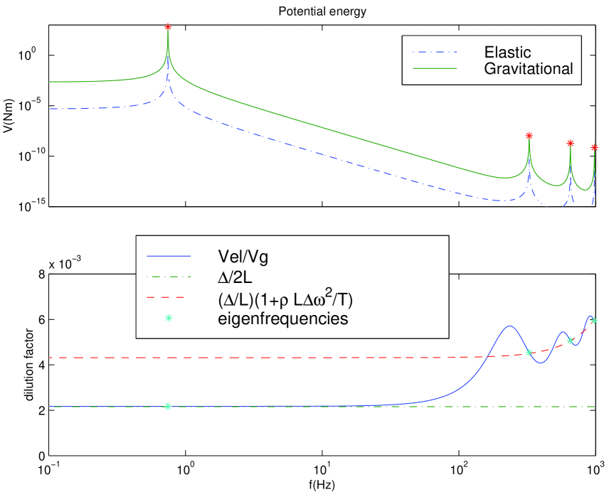
FIG. 1.: Top figure: Gravitational and potential energies for a suspended point mass as a function of frequency $f$, when excited by a sinusoidal force wiht frequency $f$. Bottom figure: ratio of energies, considered as a “dilution factor”. The stars indicate the factor $\phi/Q_{i}$, where $\phi$ is the wire loss factor and $Q_{i}$ is the eigenmode quality factor.

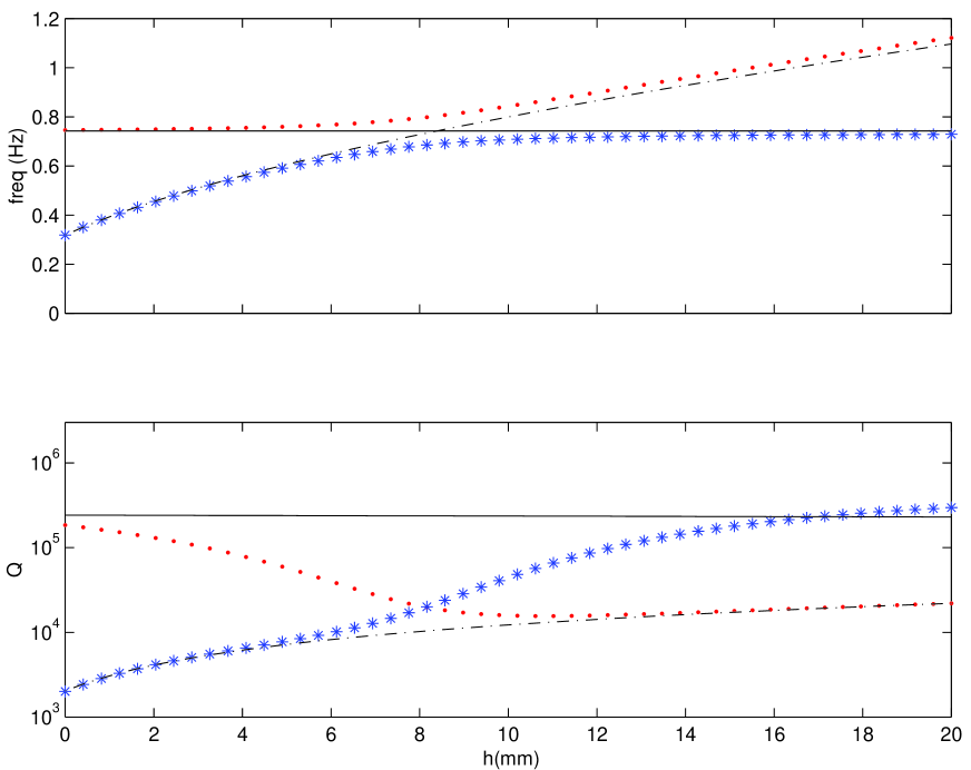
FIG. 2.: Eigenfrequencies and associated loss factors for a pendulum suspended on one wire. Quality factors and corresponding eigenfrequencies are represented with the same symbol (points or stars). The lines in the top figure are given by expressions for the pendulum frequency $f_{p}=\sqrt{g/l}/(2\pi)$ (solid) and pitch frequency $f_{\theta}=\sqrt{Th/J}/(2\pi)$ (dashed). The lines in the bottom figure correspond to the effective quality factors for displacement (solid) and for pitch (dashed). Approximate expressions for the effective quality factors are $Q_{p}\sim L/\Delta\phi$ and $Q_{\theta}\sim 2(h+\Delta)/\Delta\phi$, respectively.

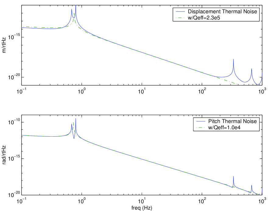
FIG. 3.: Displacement (top) and pitch (bottom) thermal noise of a single-wire pendulum, calculated without approximations (solid line), and approximated with a single mode with an effective Q (dotted line). The pitch distance used was 8.3 mm

FIG. 4.: At the top, we plot the elastic and gravitational potential energies for a pitch distance h=8.2mm. In the bottom figure, we plot the ratio of elastic and gravitational energy for three different values of the pitch distance. The stars represent the dilution factor of the pendulum mode, at the pendulum frequency; the circles are the dilution factors of the pitch mode, at the pitch eigenfrequency; and the solid horizontal line is the dilution factor of the effective quality factor at 50 Hz.

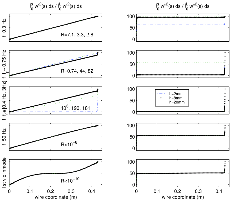
FIG. 5.: The figure shows cumulative potential energies along the wire (top is $s=0$, bottom is $s=0.45$m), when the pendulum is excited by a force a the center of mass of frequency $f$. The energies are shown for three different pitch distances in each graph: h=2mm (dashed), h=8mm (thick points) and h=20mm (dotted). The energies are also plotted for five different frequencies: $f=0.3$ Hz, below all eigenmodes; $f=f_{p}$ orpendulum frequency, approximately 0.75 Hz; $f=f_{\theta}=\sqrt{Th/J}/(2\pi)=(0.46,0.69,1.12)$Hz for $h=(2,8,20)$mm respectively; f=50Hz, in the gravitational wave band; and $f=319$Hz, the first violin mode frequency.

FIG. 6.: In the top figure, we plot the thermal noise amplitude spectral density (ASD) at 50 Hz, as a function of the distance $d$ at which the laser beam is positioned. In the middle figure, we plot the thermal noise ASD times $f^{2/5}$ obtained for $d=0$ and for the optimal distance for $f=50$Hz. In the bottom figure, we plot the ratio of the two curves in the middle figure.

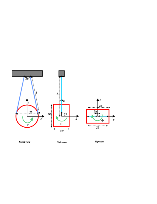
FIG. 7.: LIGO pendulum suspension, with a single wire loop, attached slightly above the center of mass and angled towards the center.

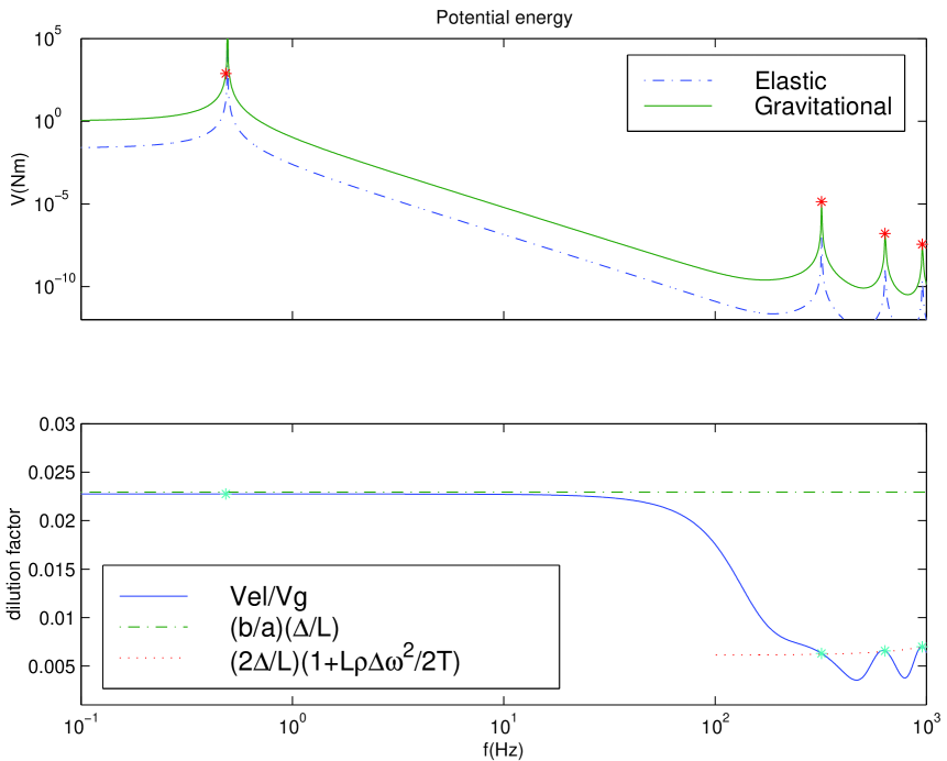
FIG. 8.: Potential energies and dilution factor for LIGO yaw degree of freedom

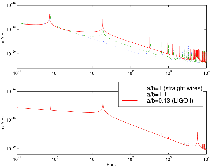
FIG. 9.: Thermal noise of pendulum side and roll motion, for different values of the distance between the wires at the top. The wires are tilted with respect to the vertical direction at an angle $\sin\alpha=(b-a)/L$, where $L$ is the length of the wires.

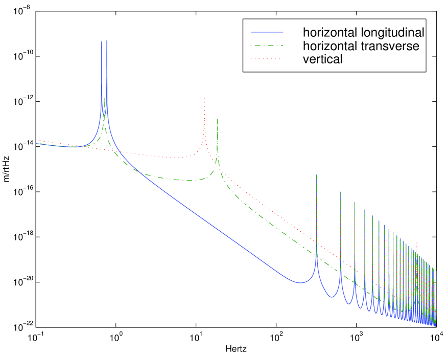
FIG. 10.: Thermal noise of the three mirror’s displacement degrees of freedom.

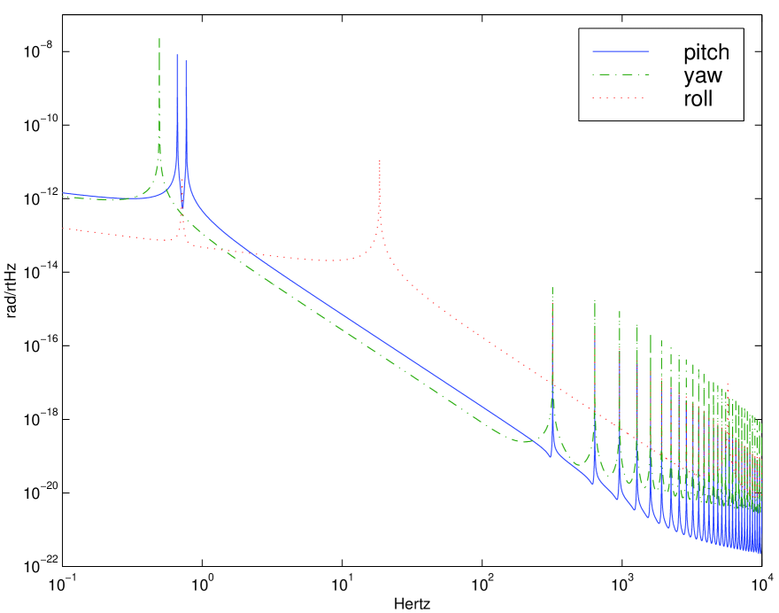
FIG. 11.: Thermal noise of the three mirror’s angular degrees of freedom.

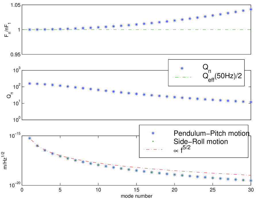
FIG. 12.: In the top figure, we show the frequencies of the resonant violin modes, scaled by $f_{n}=n\sqrt{T/rho}/2L$, for longitudinal and transverse modes. In the middle figure, we show the corresponding quality factors. The solid line is $Q_{e}ff/2\sim L/2\Delta$. In the bottom figure, we show the amplitude of longitudinal and transverse thermal noise at the violin modes. The solid line shows a $1/f^{5/2}$ fall off from the first peak.

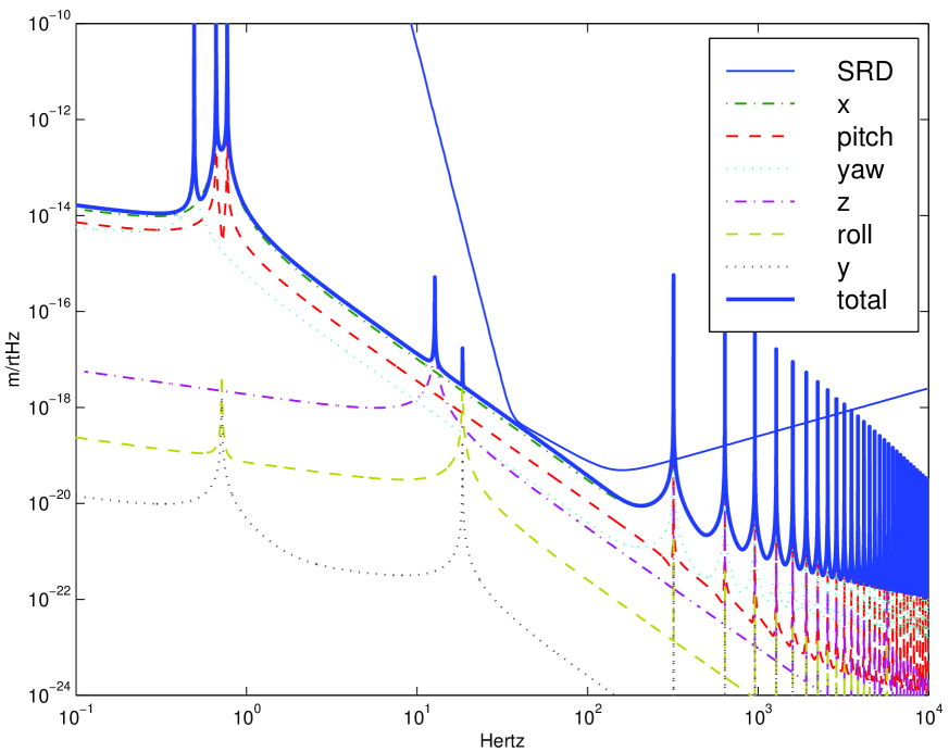
FIG. 13.: Thermal noise sensed by a laser beam 5mm away from center, and 1$\mu$rad away from horizontal. The “SRD” curve is the expected sensitivity of LIGO I. The individual degrees of freedom are plotted in their order of contribution at 100 Hz.

REFERENCES

- [1] Recent reviews of the status of interferometric gravitational waves detectors around the world can be found in the Proceedings of the Third Edoardo Amaldi Conference on Gravitational Waves, in press: M. Coles, The Status of LIGO; F. Marion, The status of the VIRGO Experiment; H. Lück, P. Aufmuth, O.S. Brozek et al.,The status of GEO600; M. Ando, K. Tsubono, TAMA Project: Design and current status; and D. McClelland, M.B. Gray et al, Status of Australian Consortium for Interferometric Gravitational Astronomy. Electronic files can be found at http://131.215.125.172/info/paperindex/
- [2] P.R. Saulson, Phys. Rev. D 40, 2437 (1990).
- [3] G.I. González and P.R. Saulson, J. Acoust. Soc. Am. 96,207 (1994).
- [4] J. Logan, J.Hough and N. Robertson, Phys. Lett. A 183,145 (1993).
- [5] V.B. Braginsky, Y. Levin, S. Vyatchanin, Measur.Sci.Tech. 10,598 (1999).
- [6] A. Gillespie and F. Raab, Phys. Lett. A 190, 213 (1994).
- [7] Matthew Hussman, Ph.D. Thesis, Uiversity of Glasgow, 2000.
- [8] S. Rowan et al., Physics Letters A, 233,303 (1997).
- [9] A. Gretarsson et al., preprint gr-qc/9912057.
- [10] Jim Hough, Peter Saulson, Mitrofanov (personal communication); Damping Dilution Factor for a pendulum in an interferometric gravitational wave detector, G. Cagnoli et al., preprint.
- [11] A. Gillespie and F. Raab, Phys. Rev. D 52, 577 (1995).
- [12] Abramovici et. al, Science 256,325 (1992). See also information on http://www.ligo.caltech.edu