On Imprisoned Curves and b-length
in General Relativity

Abstract

This paper is concerned with two themes: imprisoned curves and the b-length functional. In an earlier paper by the author, it was claimed that an endless incomplete curve partially imprisoned in a compact set admits an endless null geodesic cluster curve. Unfortunately, the proof was flawed. We give an outline of the problem and remedy the situation by providing a proof by different methods. Next, we obtain some results concerning the structure of b-length neighbourhoods, which gives a clue to how the geometry of a spacetime $(M,g)$ is encoded in the pseudo-orthonormal frame bundle equipped with the b-metric. We also show that a previous result by the author, proving total degeneracy of a b-boundary fibre in some cases, does not apply to imprisoned curves. Finally, we correct some results in the literature linking the b-lengths of general curves in the frame bundle with the b-length of the corresponding horizontal curves.

1 Introduction

In general relativity, the concept of b-length (or generalised affine parameter length) is essential, in that a spacetime is said to be singular if it contains a curve that cannot be extended to a curve with infinite b-length. This paper has two main themes: properties of the b-length functional and of imprisoned incomplete curves.

We start by giving some preliminary definitions in section 2. After that, we give some comments on the variational theory of the b-length functional. In [14], the author stated a theorem linking b-length extremals to geodesics of $(M,g)$. However, as pointed out by V. Perlick [11], the proof in [14] is flawed. It turns out that b-length extremals will not be geodesics, except in very special cases. We give an outline of the argument in section 3.

In section 4, we study cluster curves of sequences of curves with b-length tending to 0. We establish a technical result that will be used in section 5, which also allows us to settle the issue of Theorem 3 in [14]: incomplete and endless curves which are partially imprisoned in a compact set admit null geodesic cluster curves. This is in agreement with the corresponding result for totally imprisoned curves [13].

We then turn to the study of b-distance neighbourhoods in section 5, the main idea being to find information about how the geometry of $(M,g)$ is encoded in the pseudo-orthonormal frame bundle $OM$ with b-metric $G$. Since the b-length of a null geodesic segment can be made arbitrarily small by a suitable boost of the initial frame, the b-neighbourhoods of a given point contain the light cone of that point. If we restrict attention to compact sets without imprisoned null geodesics, the points on the light cone are the only ones having this property. If we allow the set to ‘touch’ the b-boundary, by allowing it to be open or to contain imprisoned curves, the situation is not so clear. We provide some illustrations by means of examples in the Minkowski, Misner and Robertson-Walker spacetimes in section 6.

In [15] it was shown that the fibre over a b-boundary point $p$ is completely degenerate, given that the frame components of the curvature and its first derivative along a horizontal curve ending at $p$ diverge sufficiently fast. Since an incomplete endless imprisoned curve ends at a b-boundary point, one might ask if the methods of [15] is applicable to that situation. In section 7 we show that this is not the case.

Finally, we give a result on the b-length of general curves in the pseudo-orthonormal frame bundle $OM$ in relation to the b-length of horizontal curves in Appendix A. In the literature, it is sometimes stated that the b-length of a horizontal curve is less than or equal to the b-length of general curve, if the two curves start at the same point in $OM$ and the projections to $M$ coincide [3, 2]. We show that this is not really the case, but that a similar estimate can be established, which is sufficient for the applications in [3] and [2].

2 Preliminaries

The basic object in general relativity is spacetime, which is a pair $(M,g)$ where $M$ is a smooth 4-dimensional connected orientable and Hausdorff manifold and $g$ is a smooth Lorentzian metric on $M$.

We need to define some concepts relating to curves $\gamma:I\to M$. Here $I$ is an interval in $\mathbb{R}$, possibly infinite. Suppose that $\gamma$ is a future directed curve and that $\mathcal{U}\subset M$. A point $p\in\mathcal{U}$ is a future endpoint of $\gamma$ if for any neighbourhood $\mathcal{V}$ of $p$ in $\mathcal{U}$ there is a parameter value $t_{0}\in I$ such that $\gamma(t)\in\mathcal{V}$ for every $t\in I$ with $t\geq t_{0}$. A curve without future endpoint in $\mathcal{U}$ is said to be future endless in $\mathcal{U}$. We also say that a geodesic $\gamma$ is future inextendible in $\mathcal{U}$ if $\gamma$ cannot be extended to the future as a geodesic in $\mathcal{U}$. In an open set, a geodesic is inextendible if and only if it is endless, while if the set isn’t open an inextendible geodesic may have endpoints on the boundary. Of course, there are obvious analogues of these definitions with ‘future’ replaced by ‘past’. We will usually leave out the temporal adjective, the direction being defined by the context.

To reduce index clutter we will, somewhat sloppily, denote a subsequence by saying that, e.g., $\{x_{j}\}$ is a subsequence of $\{x_{i}\}$. We then mean that $j$ takes values in an index set that is a subset of the index set of $i$.

We will deal extensively with sequences of curves $\{\lambda_{i}\}$. We say that $\{\lambda_{i}\}$ converges to a point if there is a point $p\in M$ such that for any neighbourhood $\mathcal{U}$ of $p$, there is an $N\in\mathbb{N}$ such that $\lambda_{i}$ is contained in $\mathcal{U}$ for all $i>N$. There is some confusion in the literature concerning the terminology used for the various concepts of convergence of a sequence of curves. Here we choose to reserve the term ‘limit’ for the stronger type of convergence which is termed ‘convergence’ in [18], and replace ‘limit’ with ‘cluster’, which the author feels is more appropriate (see also [5]). We say that $p$ is a limit point of a sequence of curves $\{\lambda_{i}\}$ if for every neighbourhood $\mathcal{U}$ of $p$, there is an $N\in\mathbb{N}$ such that $\lambda_{i}$ intersects $\mathcal{U}$ for each $i>N$. Similarly, we say that $p$ is a cluster point of $\{\lambda_{i}\}$ if every neighbourhood $\mathcal{U}$ of $p$ intersects infinitely many $\lambda_{i}$. Alternatively, a cluster point of $\{\lambda_{i}\}$ is a limit point of some subsequence of $\{\lambda_{i}\}$. A curve $\gamma$ is said to be a limit curve of $\{\lambda_{i}\}$ if all points on $\gamma$ are limit points of $\{\lambda_{i}\}$. Finally, $\gamma$ is a cluster curve of $\{\lambda_{i}\}$ if $\gamma$ is a limit curve of some subsequence of $\{\lambda_{i}\}$. Note that being a ‘cluster curve’ is a stronger restriction than being a ‘curve of cluster points’.

Next we define what is meant by imprisoned curves. A curve is said to be (past or future) totally imprisoned in a compact set $\mathcal{K}$ if it is completely contained in $\mathcal{K}$ (to the past or the future), and partially imprisoned if it intersects $\mathcal{K}$ an infinite number of times. In [5], these concepts are defined only for causal curves, but they can be applied to general curves as well. The case of interest is of course when the imprisoned curve is endless and incomplete.

To define what is meant by a curve being incomplete, we need to define what we mean by the length of a curve. Given a curve $\gamma:I\to M$ and a pseudo-orthonormal frame $E_{0}$ at some point of $\gamma$, we define the b-length or generalised affine parameter length as

$$l(\gamma,E_{0}):=\int_{I}\lvert\mathbf{V}\rvert\,\mathrm{d}t,$$ (1)

where $\lvert\mathbf{V}\rvert$ is the Euclidian norm of the component vector $\mathbf{V}$ of the tangent vector of $\gamma$ in the frame $E$ resulting from parallel propagation of $E_{0}$ along $\gamma$ [12, 5].

Because the b-length of a curve is dependent on a parallel frame along the curve, it is convenient to introduce the bundle of pseudo-orthonormal frames $OM$. $OM$ is principal fibre bundle over $M$ with the Lorentz group $\mathcal{L}$ as its structure group, and we write the right action of an element $\mathbf{L}\in\mathcal{L}$ as $R_{\mathbf{L}}\colon E\mapsto E\mathbf{L}$ for any $E\in OM$. Since $OM$ is a principal fibre bundle, there is a canonical 1-form $\boldsymbol{\theta}$ on $OM$, taking values in $\mathbb{R}^{4}$. Also, the metric on $M$ induces a connection form $\boldsymbol{\omega}$ on $OM$ which takes values in the Lie algebra $\mathfrak{l}$ of $\mathcal{L}$. Using these two forms we may define a Riemannian metric on $OM$, the Schmidt metric or b-metric, by

$$G(X,Y):=\langle\boldsymbol{\theta}(X),\boldsymbol{\theta}(Y)\rangle_{\mathbb{R}^{4}}+\langle\boldsymbol{\omega}(X),\boldsymbol{\omega}(Y)\rangle_{\mathfrak{l}},$$ (2)

where $\langle\cdot,\cdot\rangle_{\mathbb{R}^{4}}$ and $\langle\cdot,\cdot\rangle_{\mathfrak{l}}$ are Euclidian inner products with respect to fixed bases in $\mathbb{R}^{4}$ and $\mathfrak{l}$, respectively. There is still some arbitrariness in the choice of these fixed bases, but it can be shown that a change of bases transforms the b-metric to a uniformly equivalent metric [12, 3].

We now define the b-length of a general curve $\bar{\gamma}:I\to OM$ as the metric length of $\bar{\gamma}$ with respect to $G$. In other words, the b-length of  $\bar{\gamma}$ is

$$l(\bar{\gamma}):=\int_{I}\Bigl{(}\lvert\boldsymbol{\theta}(\dot{\bar{\gamma}})\rvert^{2}+\lVert{\boldsymbol{\omega}(\dot{\bar{\gamma}})}\rVert^{2}\Bigr{)}^{1/2}\,\mathrm{d}t,$$ (3)

where $\lvert\cdot\rvert$ and $\lVert{\cdot}\rVert$ are Euclidian norms in $\mathbb{R}^{4}$ and $\mathfrak{l}$, respectively, and $\dot{\bar{\gamma}}$ denotes the tangent of $\bar{\gamma}$. For horizontal curves, (3) is in agreement with the previous definition (1), in the following sense: if $\bar{\gamma}$ is the horizontal lift of a curve $\gamma$ with parallel frame $E$, then $l(\bar{\gamma})=l(\gamma,E)$. We also write $d(E,F)$ for the b-metric distance between two points $P,Q\in OM$ and $B_{r}(P)$ for the open ball in $OM$ with centre at $P$ and b-metric radius $r$.

The metric $G$ turns $(OM,G)$ into a Riemannian manifold, in particular, $OM$ is a metric space with respect to the topological metric $d$. One may therefore construct the Cauchy completion $\hskip 1.79993pt\overline{OM}$ of $OM$, and we write $\partial OM=\hskip 1.79993pt\overline{OM}\setminus OM$. By extending the right action of $\mathcal{L}$, it is possible to project $\hskip 1.79993pt\overline{OM}$ to an extension $\mathrm{cl}_{b}M$ of $M$. The b-boundary of $M$ is then defined as $\partial_{b}M=\mathrm{cl}_{b}M\setminus M$. We refer to [12], [3] or [5] for the details.

Finally, we denote the topological boundary of a set $\mathcal{U}$ by $\partial\mathcal{U}$ and the topological closure by $\overline{\mathcal{U}}$. If $\mathcal{U}$ a subset of $OM$, $\overline{\mathcal{U}}$ means the usual closure of $\mathcal{U}$ in $OM$ and not in the Cauchy completion $\hskip 1.79993pt\overline{OM}$, unless stated otherwise.

3 Imprisoned curves and variations of b-length

In [14], the author studied local variations of the b-length functional (1), the primary purpose being to apply the result to imprisoned curves. The result was that in sufficiently small globally hyperbolic sets, causal curves of minimal b-length are geodesics. However, this statement is false, and there is an error in the main argument of [14], as pointed out by V. Perlick [11]. We give an outline of the argument here, this section being completely due to V. Perlick. The author of this paper accepts the responsibility for any errors, of course.

For the moment, we disregard the presence of a Lorentz metric $g$ and view $M$ as a smooth manifold with smooth connection $\nabla$ and without torsion. Let $p,q\in M$ and fix a frame $E_{p}$ at $p$. We consider a variational principle where the trial paths are smooth curves of the form $\lambda\colon[0,a]\to M$ from $p$ to $q$, and the functional to be extremised is the b-length $l(\lambda,E_{p})$, given by (1).

Proposition 3.1.

Let $\lambda\colon[0,a]\to M$ be a curve from $p$ to $q$ in $M$. Without loss of generality we may assume that $\lambda$ is parameterised by b-length $t$. Let $\mathbf{V}^{i}$ and $\mathbf{R}^{i}\!_{jkl}$ be the components of the tangent of $\lambda$ and the Riemann tensor, respectively, in the frame $E$ obtained by parallel propagation of $E_{p}$ along $\lambda$. Then $\lambda$ is an extremal of the b-length functional only if

$$\dot{\mathbf{V}}^{i}=\delta^{im}\mathbf{Q}^{k}\!_{j}\,\mathbf{R}^{j}\!_{klm}\mathbf{V}^{l},$$ (4)

where the dot denotes a derivative with respect to $t$ and $\mathbf{Q}^{i}\!_{k}(t)$ is the solution of the initial value problem

$$\dot{\mathbf{Q}}^{i}\!_{k}=\mathbf{V}^{i}\mathbf{V}^{j}\delta_{jk},\qquad\mathbf{Q}^{i}\!_{k}(a)=0.$$ (5)

Proof.

With a slight abuse of notation, we consider $\lambda$ to be a 1-parameter family of curves with variational parameter $u$, such that $u=0$ corresponds to the original curve. The variational vector field $X:=\frac{\partial}{\partial u}$ is assumed to be smooth with boundary conditions $X(0,u):=0$ and $X(a,u):=0$. Parallel propagation of $E_{p}$ along $\lambda$ for each fixed $u$ gives a frame field $E(t,u)$, and a coframe field $\theta(t,u)$ dual to $E(t,u)$. We also denote a $t$-derivative by a dot and write $V$ for the tangent of $\lambda$. The b-length functional (1) can then be written as

$$l(\lambda,E_{p})=\int_{0}^{a}\lvert\theta(V)\rvert\,\mathrm{d}t.$$ (6)

Note that if $\bar{\lambda}$ is the horizontal lift of $\lambda$ for each fixed $u$, then the lift of $\theta$ coincides with the canonical 1-form $\boldsymbol{\theta}$, so (6) agrees with the definition (3) of b-length for horizontal curves in $OM$.

Differentiating (6) and evaluating at $u=0$, we get

$$\begin{split}\frac{\mathrm{d}}{\mathrm{d}u}l(\lambda,E_{p})&=\int_{0}^{a}\lvert\theta(V)\rvert^{-1}\delta_{ij}\theta^{i}(V)\frac{\partial}{\partial u}\bigl{(}\theta^{j}(V)\bigr{)}\,\mathrm{d}t\\ &=\int_{0}^{a}\mathbf{V}^{i}\bigl{(}(\nabla_{X}\theta^{j})(V)+\theta^{j}(\nabla_{X}V)\bigr{)}\,\mathrm{d}t\end{split}$$ (7)

where we have used that $\lvert\theta(V)\rvert=1$ since $\lambda$ is parameterised by b-length at $u=0$, and the indices $i,j,k,\dots$ denote components in the frame $E$. Using that $V=\mathbf{V}^{i}E_{i}$ and $[V,X]=0$,

$$\begin{split}\frac{\mathrm{d}}{\mathrm{d}u}l(\lambda,E_{p})&=\int_{0}^{a}\delta_{ij}\mathbf{V}^{i}\bigl{(}\mathbf{V}^{k}(\nabla_{X}\theta^{j})(E_{k})+\theta^{j}(\nabla_{V}X)\bigr{)}\,\mathrm{d}t\\ &=\int_{0}^{a}\delta_{ij}\mathbf{V}^{i}\bigl{(}-\mathbf{V}^{k}\theta^{j}(\nabla_{X}E_{k})+\frac{\mathrm{d}}{\mathrm{d}t}(\mathbf{X}^{j})\bigr{)}\,\mathrm{d}t,\end{split}$$ (8)

since $\nabla_{X}\bigl{(}\theta^{j}(E_{k})\bigr{)}=0$ and $\nabla_{V}\theta^{j}=0$. Rewrite $\theta^{j}(\nabla_{X}E_{k})$ as an integral from 0 to $t$ and perform a partial integration on the second term. Then

$$\frac{\mathrm{d}}{\mathrm{d}u}l(\lambda,E_{p})=-\int_{0}^{a}\delta_{ij}\mathbf{V}^{i}\mathbf{V}^{k}\int_{0}^{t}\mathbf{R}^{j}\!_{klm}\mathbf{V}^{l}\mathbf{X}^{m}\,\mathrm{d}\hat{t}\,\mathrm{d}t-\int_{0}^{a}\delta_{ij}\dot{\mathbf{V}}^{i}\mathbf{X}^{j}\,\mathrm{d}t.$$ (9)

To proceed further we define $\mathbf{Q}^{i}\!_{k}(t)$ as the solution of the initial value problem (5). We can then partially integrate the first term in (9), which results in

$$\frac{\mathrm{d}}{\mathrm{d}u}l(\lambda,E_{p})=\int_{0}^{a}\bigl{(}\mathbf{Q}^{i}\!_{j}\mathbf{R}^{j}\!_{ilm}\mathbf{V}^{l}-\dot{\mathbf{V}}^{i}\delta_{im}\bigr{)}\mathbf{X}^{m}\,\mathrm{d}t.$$ (10)

By the basic principle of variational calculus, we arrive at condition (4). ∎

Based on Proposition 3.1, we can make some remarks on b-length extremals:

1. Given a value for $\mathbf{V}(a)$, (4) and (5) determine unique solutions for $\mathbf{V}$ and $\mathbf{Q}$ on some interval $[a-\epsilon,a]$. So any point $q$ has a neighbourhood $\mathcal{U}$ such that a b-length extremal from $p$ to $q$ exists for all $p\in\mathcal{U}$.

2. The two equations (4) and (5) may be viewed as an integro-differential equation for $\mathbf{V}$. Thus the situation is qualitatively different from that of geodesics in $M$, which are solutions to a single system of 4 ordinary differential equations. Alternatively, reformulating the problem in $OM$ as to find horizontal curves with extremal b-length, (4) and (5) may be viewed as a single system of 10 ordinary differential equations. There is a clear analogy to the system of 10 geodesic equations in $OM$. Hence it is probably more natural and convenient to study b-length extremals in the frame bundle context.

3. Since $\mathbf{Q}(a)=0$, (4) requires $\dot{\mathbf{V}}(a)=0$. So the acceleration $\nabla_{V}V$ has a zero at the end point $t=a$. It follows that the restriction of a b-length extremal to a subinterval is not a b-length extremal in general, since that requires that the acceleration $\nabla_{V}V$ vanishes at the endpoint of the subinterval. This is not surprising, as varying a curve on a subinterval $[0,b]\subset[0,a]$ affects the frame $E$ not only on $[0,b]$ but also on $[b,a]$.

4. The choice of the initial frame $E_{p}$ is crucial, as is evident from (4).

If $\lambda$ is a geodesic, the $\mathbf{V}^{i}$ are constant so (5) can be integrated, which results in

$$\mathbf{Q}^{i}\!_{k}(t)=\mathbf{V}^{i}\mathbf{V}^{j}\delta_{jk}(t-a).$$ (11)

Inserting this into condition (4) in Proposition 3.1 we obtain the following corollary.

Corollary 3.2.

Let $\lambda$ and $E$ be as in Proposition 3.1. Then $\lambda$ is a geodesic only if

$$\delta_{ij}\mathbf{V}^{i}\mathbf{R}^{j}\!_{klm}\mathbf{V}^{k}\mathbf{V}^{l}=0.$$ (12)

Note that (12) is algebraic, so if it is violated at one point then it is also violated on any interval containing that point.

We now turn to the case where $\nabla$ is the Levi-Cività connection of a Lorentzian metric $g$, and the frame $E_{p}$ is chosen to be pseudo-orthonormal with respect to $g$. Then the parallel frame $E$ is also pseudo-orthonormal along any of the trial paths, so for all vector fields $X$ and $Y$,

$$\mathbf{X}^{i}\mathbf{Y}^{j}\delta_{ij}=g(X,Y)+2\,g(E_{0},X)\,g(E_{0},Y),$$ (13)

where $E_{0}$ is the timelike vector of the frame $E$. By Corollary 3.2, a b-length extremal is a geodesic only if

$$\mathbf{V}^{i}\mathbf{R}_{iklm}\mathbf{V}^{k}\mathbf{V}^{l}+2\,\mathbf{V}^{0}\mathbf{R}_{0klm}\mathbf{V}^{k}\mathbf{V}^{l}=0.$$ (14)

By the symmetries of the curvature tensor $R$, the first term vanishes, and if $\lambda$ is causal, $\mathbf{V}^{0}\neq 0$. Thus a causal b-length extremal is a geodesic only if

$$\mathbf{R}_{0klm}\mathbf{V}^{k}\mathbf{V}^{l}=0.$$ (15)

It is apparent that (15) may be satisfied for some choice of $E_{p}$ and violated for some other choice. We wish to investigate if it is possible to choose $E_{p}$ such that all sufficiently short causal b-length extremals starting at $p$ are geodesics. Since the causal vectors span the whole tangent space, (15) shows that this is possible if and only if

$$0=\mathbf{R}_{0klm}-\mathbf{R}_{0lkm}=-\mathbf{R}_{ml0k}+\mathbf{R}_{mk0l}=\mathbf{R}_{m0kl},$$ (16)

because of the curvature identities. Clearly, (16) holds only if $\mathbf{R}_{0l}=0$, i.e., the Ricci tensor $\mathbf{R}_{ij}$ must be degenerate. This is of course an exceptional case not satisfied by a generic spacetime.

Finally, the results in this section is obviously in conflict with Lemma 3 of [14], which states that a non-geodesic causal curve in spacetime cannot be a b-length extremal. This claim is incorrect. As outlined in the proof, any non-geodesic smooth curve $\lambda$ may be restricted to a subinterval where the acceleration is bounded away from zero, and the restriction of $\lambda$ cannot be a b-length extremal. However, as we have noted in remark 3 above, this does not imply that the whole curve cannot be a b-length extremal. What is shown in Lemma 3 of [14] is in fact that the acceleration cannot be bounded away from zero on a b-length extremal. The reason is, as we have seen, that the acceleration must have a zero at the end point.

It follows that Theorem 2 of [14] is incorrect as well. If $M$ admits a covariantly constant timelike vector field $E_{0}$ with $g(E_{0},E_{0})=-1$, Lemma 3 and Theorem 2 may be reestablished, but that is a non-generic situation.

The remaining result of [14], Theorem 3, may be reestablished by other means, which we will do in section 4.

4 Cluster curves

This section is devoted to the study of cluster curves, the main goal being to reestablish Theorem 3 of [14], which states that a partially imprisoned incomplete endless curve has an endless null geodesic cluster curve (see Theorem 4.2 below). First we need a technical result, which will also be used in section 5.

Lemma 4.1.

Let $\mathcal{U}\subset M$ and suppose that $p\in\mathcal{U}$ is a cluster point of a family of incomplete endless curves $\{\lambda_{i}\}$ in $\mathcal{U}$, with horizontal lifts $\{\bar{\lambda}_{i}\}$ satisfying $l(\bar{\lambda}_{i})\to 0$ as $i\to\infty$. If $\{\lambda_{i}\}$ has no subsequence that converges to a point in the topological closure $\overline{\mathcal{U}}$, then there is an inextendible null geodesic cluster curve of $\{\lambda_{i}\}$ through $p$ in $\overline{\mathcal{U}}$.

Proof.

We may assume that $\bar{\lambda}_{i}\colon[0,1)\to OM$. Suppose that $\{\bar{\lambda}_{i}\}$ has a cluster point $y\in OM$. Then there is a sequence $\{t_{j}\}$ of real numbers such that$y_{j}:=\bar{\lambda}_{j}(t_{j})\to y$. Let $\mathcal{V}$ be an arbitrarily small neighbourhood of $\pi(y)$ in $M$. Then there is a small ball $B_{r}(y)$ around $y$ in $OM$ such that $\pi(B_{r}(y))\subset\mathcal{V}$. But $l(\bar{\lambda}_{i})\to 0$, so there is an $N\in\mathbb{N}$ such that $\bar{\lambda}_{j}$ is contained in $B_{r}(y)$ for all $j\geq N$. Then $\lambda_{j}$ is contained in $\mathcal{V}$ for all $j\geq N$, so $\{\lambda_{j}\}$ converges to $\pi(y)$ which contradicts the assumption on $\{\lambda_{i}\}$.

Since $p$ is a cluster point of $\{\lambda_{i}\}$, there is a sequence $\{t_{j}\}$ such that$p_{j}:=\lambda_{j}(t_{j})\to p$. Put $\bar{p}_{\!j}:=\bar{\lambda}_{j}(t_{j})$. By the argument in the previous paragraph, $\{\bar{p}_{\!j}\}$ has no cluster point in $OM$. Let $\mathcal{V}$ be a convex normal neighbourhood of $p$ in $M$, let $\sigma\colon\mathcal{V}\to OM$ be a cross-section of $OM$ over $\mathcal{V}$, and let $\tilde{\lambda}_{j}(t):=\sigma\circ\lambda_{j}(t)$ whenever $\lambda_{j}(t)\in\mathcal{V}$. The action of $\mathcal{L}$ on $OM$ is free and transitive, so there are unique matrices $\mathbf{L}_{j}(t)\in\mathcal{L}$ such that in $\pi^{-1}(\mathcal{V})$,

$$\bar{\lambda}_{j}(t)=\tilde{\lambda}_{j}(t)\mathbf{L}_{j}(t).$$ (17)

$\mathbf{L}_{j}(t)$ may be decomposed as $\mathbf{L}_{j}(t)=\bar{\boldsymbol{\Omega}}_{j}(t)\boldsymbol{\Lambda}_{j}(t)\boldsymbol{\Omega}_{j}(t)$, where $\boldsymbol{\Omega}_{j}(t)$ and $\bar{\boldsymbol{\Omega}}_{j}(t)$ are spatial rotations and

$$\boldsymbol{\Lambda}_{j}(t):=\begin{bmatrix}\cosh\xi_{j}(t)&\sinh\xi_{j}(t)&0&0\\ \sinh\xi_{j}(t)&\cosh\xi_{j}(t)&0&0\\ 0&0&1&0\\ 0&0&0&1\end{bmatrix}$$ (18)

is a Lorentz boost by a hyperbolic angle $\xi_{j}(t)\in\mathbb{R}$. Let $\bar{\xi}_{j}:=\xi_{j}(t_{j})$. If $\lvert\bar{\xi}_{j}\rvert$ had an upper bound $\xi_{0}<\infty$, then $\{\bar{p}_{\!j}\}$ would be contained in a compact subset of $OM$, which is impossible since $\{\bar{p}_{\!j}\}$ has no cluster point. We therefore assume that $\sup\{\bar{\xi}_{j}\}=\infty$, the case when $\inf\{\bar{\xi}_{j}\}=-\infty$ being similar.

Now $O(3)$ is compact, so there is a subsequence $\{\bar{p}_{\!k}\}$ of $\{\bar{p}_{\!j}\}$ such that$\xi_{k}\to\infty$, $\boldsymbol{\Omega}_{k}(t_{k})\to\boldsymbol{\Omega}_{0}$ and $\bar{\boldsymbol{\Omega}}_{k}(t_{k})\to\bar{\boldsymbol{\Omega}}_{0}$ as $k\to\infty$. Let

$$\lambda_{k}^{\prime}(t):=\bar{\lambda}_{k}(t)\boldsymbol{\Omega}_{k}(t_{k})^{-1}=\tilde{\lambda}_{k}(t)\bar{\boldsymbol{\Omega}}_{k}(t)\boldsymbol{\Lambda}_{k}(t)\boldsymbol{\Omega}_{k}(t)\boldsymbol{\Omega}_{k}(t_{k})^{-1}$$ (19)

and

$$\hat{\lambda}_{k}(t):=\bar{\lambda}_{k}(t)\boldsymbol{\Omega}_{k}(t_{k})^{-1}\boldsymbol{\Lambda}_{k}(t_{k})^{-1}=\tilde{\lambda}_{k}(t)\bar{\boldsymbol{\Omega}}_{k}(t)\boldsymbol{\Lambda}_{k}(t)\boldsymbol{\Omega}_{k}(t)\boldsymbol{\Omega}_{k}(t_{k})^{-1}\boldsymbol{\Lambda}_{k}(t_{k})^{-1}.$$ (20)

Then

$$\hat{\lambda}_{k}(t_{k})=\tilde{\lambda}_{k}(t_{k})\bar{\boldsymbol{\Omega}}_{k}(t_{k})\to\hat{p}:=\sigma(p)\bar{\boldsymbol{\Omega}}_{0}$$ (21)

as $k\to\infty$. Since $\boldsymbol{\Omega}_{k}(t_{k})$ is a constant rotational matrix, leaving the Euclidian norm invariant, it does not affect the length of $\lambda_{k}^{\prime}$. From $l(\bar{\lambda}_{k})\to 0$ it follows that $l(\lambda_{k}^{\prime})\to 0$ and so

$$\int_{t_{k}}^{1}\lvert\mathbf{X}_{k}^{I}\rvert\,\mathrm{d}t\to 0,\qquad I=u,v,2,3,$$ (22)

where $\mathbf{X}_{k}^{I}:=G(E_{I},\dot{\lambda}_{k}^{\prime})$, $E_{u}:=\tfrac{1}{\sqrt{2}}(E_{0}+E_{1})$, $E_{v}:=\tfrac{1}{\sqrt{2}}(E_{0}-E_{1})$ and $E_{0}$, $E_{1}$, $E_{2}$ and $E_{3}$ are the standard horizontal vector fields on $OM$ [7]. Similarly, let $\mathbf{Y}_{k}^{I}=G(E_{I},\dot{\hat{\lambda}}_{k})$. Then $\mathbf{Y}_{k}^{u}=e^{\xi_{k}}\mathbf{X}^{u}$, $\mathbf{Y}_{k}^{v}=e^{-\xi_{k}}\mathbf{X}^{v}$, $\mathbf{Y}_{k}^{2}=\mathbf{X}^{2}$ and $\mathbf{Y}_{k}^{3}=\mathbf{X}^{3}$, so

$$\int_{t_{k}}^{1}\lvert\mathbf{Y}_{k}^{I}\rvert\,\mathrm{d}t\to 0,\qquad I=v,2,3.$$ (23)

Let $\bar{\mu}$ be the integral curve of $E_{u}$ through $\hat{p}$. Then $\mu:=\pi\circ\bar{\mu}$ is a null geodesic in $\mathcal{V}$. We may assume that $\bar{\mu}$ is extended as far as possible as the horizontal lift of an unbroken null geodesic in $\mathcal{V}$. We show that $\bar{\mu}$ is a limit curve of $\{\hat{\lambda}_{k}\}$. Let $q$ be a point on $\bar{\mu}$, let $\mathcal{W}$ be a neighbourhood of $q$ in $\pi^{-1}(\mathcal{V})$, and let $\mathcal{T}$ be the tubular subset of $\pi^{-1}(\mathcal{V})$ generated by all integral curves of $E_{u}$ intersecting $\mathcal{W}$. Since $p\in\mathcal{T}$, (23) gives that there is an $N\in\mathbb{N}$ such that if $k>N$ then $\hat{\lambda}_{k}\cap\pi^{-1}(\mathcal{V})$ is contained in $\mathcal{T}$, i.e., $\hat{\lambda}_{k}$ does not leave $\mathcal{T}$ except possibly at the ends $\partial\bigl{(}\pi^{-1}(\mathcal{V})\bigr{)}\cap\mathcal{T}$. Now $\mathcal{V}$ does not contain any imprisoned incomplete curves since it is a convex normal neighbourhood, so $\hat{\lambda}_{k}$, having no endpoint in $\mathcal{T}\subset\mathcal{V}$, must leave $\mathcal{T}$. Thus $\hat{\lambda}_{k}$ intersects $\mathcal{W}$ for each $k>N$, which means that $q$ is a limit point of $\{\hat{\lambda}_{k}\}$.

Obviously, $\mu$ is contained in $\overline{\mathcal{U}}$ since it is a limit curve of $\{\lambda_{k}\}$. It remains to show that $\mu$ can be extended to an inextendible null geodesic cluster curve of $\{\bar{\lambda}_{i}\}$ in the whole of  $\overline{\mathcal{U}}$. Extend $\mu$ as far as possible as an unbroken null geodesic in $\overline{\mathcal{U}}$, and let $q$ be a point on $\mu$. Then the segment of $\mu$ from $p$ to $q$ is closed and finite, so it can be covered by a finite sequence of convex normal neighbourhoods $\{\mathcal{V}_{n}\}$ with $\mathcal{V}_{1}=\mathcal{V}$. By the above argument, $\mu\cap\pi^{-1}(\mathcal{V}_{1})$ is a limit curve of some subsequence $\{\bar{\lambda}_{k}\}$ of $\{\bar{\lambda}_{i}\}$. Assume that $\mu\cap\pi^{-1}(\mathcal{V}_{n})$ is a limit curve of a subsequence $\{\bar{\lambda}_{k_{n}}\}$ for some $n$. Then any point $p_{n}$ on $\mu\cap\pi^{-1}(\mathcal{V}_{n})\cap\pi^{-1}(\mathcal{V}_{n+1})$ is a cluster point. Repeating the argument with $p_{n}$ in place of $p$ and $\mathcal{V}_{n+1}$ in place of  $\mathcal{V}$ shows that $\mu\cap\pi^{-1}(\mathcal{V}_{n+1})$ is a limit curve of some subsequence $\{\bar{\lambda}_{k_{n+1}}\}$ as well. By induction, the whole curve $\mu$ is a cluster curve of $\{\bar{\lambda}_{i}\}$. ∎

The proof of Lemma 4.1 uses a similar technique as the proof of the theorem in [13], except that we have weakened the assumption of total imprisonment to a family of curves with lengths going to 0, not converging to a point. This allows us to use Lemma 4.1 in other contexts. See also Proposition 8.3.2 in [5], but note that there are some minor errors in that version.

It is now a simple matter to apply Lemma 4.1 to imprisoned curves, which allows us to settle the issue from [14] with the following theorem.

Theorem 4.2.

An incomplete endless curve partially imprisoned in a compact set admits an endless null geodesic cluster curve.

Proof.

If $\lambda$ is an incomplete endless curve partially imprisoned in a compact set $\mathcal{K}$, then the intersection of $\lambda$ with the interior of $\mathcal{K}$ is a family of incomplete endless curves $\{\lambda_{i}\}$ with horizontal lifts whose lengths go to 0. The problem is the endpoints of $\{\lambda_{i}\}$ on $\partial\mathcal{K}$, and also the possibility that $\{\lambda_{i}\}$ contains subsequences converging to a point on $\partial\mathcal{K}$ (see section 2). But this can be dealt with by enlarging $\mathcal{K}$ around any such points. Thus Lemma 4.1 gives us an inextendible null geodesic cluster curve $\gamma$ of $\{\lambda_{i}\}$ in $\mathcal{K}$. Let $\mu$ be the endless extension of $\gamma$ as a null geodesic in $M$ and let $q$ be a point on $\mu$. Then the segment of $\mu$ from $\mathcal{K}$ to $q$ is finite and so it can be included in a larger compact set $\mathcal{K}^{\prime}$. Applying Lemma 4.1 to $\mathcal{K}^{\prime}$ we find that the part of $\mu$ in $\mathcal{K}^{\prime}$ is a cluster curve of $\{\lambda_{i}\}$ as well, and since $q$ was arbitrary, the whole of $\mu$ is a cluster curve in $\mathcal{K}$. ∎

5 b-neighbourhoods and light cones

In this section we will study how the light cone structure of $(M,g)$ is encoded in $(OM,G)$. We also define a family of sets $\mathcal{N}_{p,\epsilon}(\mathcal{U})$ that effectively describe neighbourhoods within a finite b-distance from a fixed point. We start with a definition.

Definition 5.1.

Given $\mathcal{U}\subset M$ and $p,q\in\mathcal{U}$, let

$$\tilde{d}_{\mathcal{U}}(p,q):=\inf\{l(\mu);\;\mu\colon[0,1]\to\pi^{-1}(\mathcal{U}),\pi\circ\mu(0)=p,\pi\circ\mu(1)=q\}.$$ (24)

$\tilde{d}_{\mathcal{U}}$ is not a metric on $\mathcal{U}$, since it is quite possible that $\tilde{d}_{\mathcal{U}}(p,q)=0$ with $p\neq q$. Neither is it a semimetric in general, since the triangle inequality can be violated. The case of interest is sets where $\tilde{d}$ is small, in the following sense:

Definition 5.2.

Given $\mathcal{U}\subset M$, $p\in\mathcal{U}$ and $\epsilon>0$, let

$$\mathcal{N}_{p,\epsilon}(\mathcal{U}):=\{q\in\mathcal{U};\;\tilde{d}_{\mathcal{U}}(p,q)<\epsilon\}$$ (25)

and

$$\mathcal{N}_{p}(\mathcal{U}):=\{q\in\mathcal{U};\;\tilde{d}_{\mathcal{U}}(p,q)=0\}.$$ (26)

It is clear from the definition of $\tilde{d}$ that

$$\mathcal{N}_{p}(\mathcal{U})=\bigcap_{\epsilon>0}\,\mathcal{N}_{p,\epsilon}(\mathcal{U}).$$ (27)

Also, if $\epsilon_{1}<\epsilon_{2}$, $\mathcal{N}_{p,\epsilon_{1}}(\mathcal{U})\subset\mathcal{N}_{p,\epsilon_{2}}(\mathcal{U})$. When $\mathcal{U}=M$, we will write $\mathcal{N}_{p}$ instead of $\mathcal{N}_{p}(M)$.

If $q\in\mathcal{N}_{p}(\mathcal{U})$ there is a family of curves $\{\bar{\lambda}_{i}\}$ from $\pi^{-1}(p)$ to $\pi^{-1}(q)$ in $OM$ such that $l(\bar{\lambda}_{i})\to 0$ as $i\to\infty$. We will refer to such a family of curves as defining for $q\in\mathcal{N}_{p}(\mathcal{U})$. Because of Proposition A.1 in Appendix A, we can assume that the $\bar{\lambda}_{i}$ are horizontal. In fact, we could have used horizontal curves from the outset with similar results: if we replace $\tilde{d}$ with

$$\bar{d}_{\mathcal{U}}(p,q):=\inf\{l(\mu);\;\mu\colon[0,1]\to\pi^{-1}(\mathcal{U}),\pi\circ\mu(0)=p,\pi\circ\mu(1)=q,\operatorname{ver}\dot{\mu}=0\}$$ (28)

and $\mathcal{N}_{p,\epsilon}(\mathcal{U})$ with

$$\bar{\mathcal{N}}_{p,\epsilon}(\mathcal{U}):=\{q\in\mathcal{U};\;\bar{d}_{\mathcal{U}}(p,q)<\epsilon\},$$ (29)

then Proposition A.1 implies that

$$\mathcal{N}_{p,\epsilon}(\mathcal{U})\subset\bar{\mathcal{N}}_{p,(e^{\epsilon}-1)}(\mathcal{U}).$$ (30)

The sets $\bar{\mathcal{N}}_{p,\epsilon}(\mathcal{U})$ are usually somewhat easier to work with since one can then restrict attention to horizontal curves.

Proposition 5.3.

The lightcone $N_{p}(\mathcal{U})$, consisting of all points connected to $p$ by null geodesics in $\mathcal{U}$, is contained in $\mathcal{N}_{p}(\mathcal{U})$.

Proof.

Let $\gamma\colon[0,1]\to\mathcal{U}$ be a null geodesic from $p$ to $q$ with affine parameter $t$. Pick a pseudo-orthonormal frame $E$ at $p$ such that $\dot{\gamma}=(a/\sqrt{2})(E_{0}+E_{1})$ at $p$, and parallel propagate $E$ along $\gamma$. The length of $\gamma$ in the frame $E$ is

$$l(\gamma,E)=\int_{0}^{1}a\,\mathrm{d}t=a.$$ (31)

Now let $\mathbf{L}\in\mathcal{L}$ be a boost in the $E_{0}+E_{1}$ direction by hyperbolic angle $\xi$, i.e.,

$$\mathbf{L}:=\begin{bmatrix}\cosh\xi&\sinh\xi&0&0\\ \sinh\xi&\cosh\xi&0&0\\ 0&0&1&0\\ 0&0&0&1\end{bmatrix}$$ (32)

in the frame $E$. Then the length of $\gamma$ in the frame $E\mathbf{L}$ is $ae^{-\xi}$, which tends to 0 as $\xi\to\infty$. ∎

Proposition 5.3 gives a characterisation of some of the points in $\mathcal{N}_{p}(\mathcal{U})$. Using Lemma 4.1, we can also say the following about $\mathcal{N}_{p}(\mathcal{U})$.

Theorem 5.4.

$\mathcal{N}_{p}(\mathcal{U})$ is generated by inextendible null geodesics in $\mathcal{U}$.

Proof.

Let $q$ be a point in $\mathcal{N}_{p}(\mathcal{U})\setminus\{p\}$ and let $\{\bar{\lambda}_{i}\}$ be a defining family of curves for $q$. Since we may remove any loops at $p$, the projections $\lambda_{i}$ to $M$ are incomplete and endless curves in $\mathcal{U}\setminus\{p\}$. Also, $p\neq q$ so no subsequence of ${\lambda_{i}}$ converges to a point. Thus Lemma 4.1 with $q$ in place of $p$ implies that there is an inextendible null geodesic cluster curve $\gamma$ of some subsequence $\{\lambda_{k}\}$ through $q$ in $\overline{\mathcal{U}}$. Let $\gamma^{\prime}$ be the inextendible segment of $\gamma$ through $q$ in $\mathcal{U}$. We show that $\gamma^{\prime}$ is contained in $\mathcal{N}_{p}(\mathcal{U})$. Suppose that $r$ is a point on $\gamma^{\prime}$ and let $\tilde{\gamma}$ be the segment of $\gamma^{\prime}$ from $q$ to $r$. We may assume that $\tilde{\gamma}$ is parameterised by an affine parameter $t$ ranging from $0$ to $a$. As in the proof of Lemma 4.1, there is a pseudo-orthonormal frame $E$ at $q$ in which the tangent of $\tilde{\gamma}$ is $E_{u}:=\tfrac{1}{\sqrt{2}}(E_{0}+E_{1})$, and $\bar{\lambda}_{k}$ intersects $\pi^{-1}(q)$ at the frame $F:=E\boldsymbol{\Lambda}_{k}\boldsymbol{\Omega}_{k}$. Let $\bar{\gamma}_{k}$ be the horizontal lift of $\tilde{\gamma}$ to $F$. Then the component vector $\mathbf{V}$ of $\dot{\bar{\gamma}}_{k}$ with respect to the standard horizontal vector fields on $OM$ is

$$\mathbf{V}=\tfrac{1}{\sqrt{2}}\,\boldsymbol{\Omega}_{k}^{-1}\boldsymbol{\Lambda}_{k}^{-1}\!\begin{bmatrix}1\\ 1\\ 0\\ 0\end{bmatrix}.$$ (33)

Since $\boldsymbol{\Omega}_{k}$ is a rotation leaving $E_{u}$ fixed and $\boldsymbol{\Lambda}_{k}$ is a boost in the $E_{u}$ direction with hyperbolic angle $\xi_{k}$, the Euclidian norm of  $\mathbf{V}$ is

$$\lvert\mathbf{V}\rvert=e^{-\xi_{k}},$$ (34)

so the b-length of $\bar{\gamma}_{k}$ is $ae^{-\xi_{k}}$. It follows that the concatenation of $\bar{\lambda}_{k}$ and $\bar{\gamma}_{k}$ is a curve from $\pi^{-1}(p)$ to $\pi^{-1}(r)$ with length $l(\bar{\lambda}_{k})+ae^{-\xi_{k}}$, which tends to 0 as $k\to\infty$. ∎

The following theorem gives some idea of in which situations $\mathcal{N}_{p}(\mathcal{U})$ can be expected to contain more than the light cone $N_{p}(\mathcal{U})$.

Theorem 5.5.

If  $\mathcal{U}$ is a compact subset of $M$ without totally imprisoned null geodesics, then $\mathcal{N}_{p}(\mathcal{U})=N_{p}(\mathcal{U})$ for any $p\in\mathcal{U}$.

Proof.

Let $q\in\mathcal{N}_{p}(\mathcal{U})\setminus\{p\}$ and let $\{\bar{\lambda}_{i}\}$ be a defining family of curves for $q$. Since $p\neq q$, no subsequence of $\{\pi\circ\bar{\lambda}_{i}\}$ converges to a point. By Lemma 4.1, there is a null geodesic limit curve $\gamma$ of a subsequence $\{\pi\circ\bar{\lambda}_{k}\}$ of $\{\pi\circ\bar{\lambda}_{i}\}$ through $q$ in $\mathcal{U}$ which is inextendible in $\mathcal{U}\setminus\{q\}$. We assume that $\gamma$ never reaches $p$ and show that this leads to a contradiction.

Since there are no totally imprisoned null geodesics in $\mathcal{U}$, $\gamma$ must have an endpoint $r$ on $\partial\mathcal{U}$. Then $r$ is a limit point of $\{\bar{\lambda}_{k}\}$. Let $\mathcal{V}$ be a convex normal neighbourhood of $r$, sufficiently small for $p$ and $q$ not to be in $\mathcal{V}$. Each curve $\bar{\lambda}_{k}$ must enter and leave $\mathcal{V}$ for large enough $k$. By Lemma 4.1 there is an endless null geodesic cluster curve of $\{\bar{\lambda}_{k}\}$ through $r$ in $\mathcal{V}$. But every $\bar{\lambda}_{k}$ is contained in $\mathcal{U}$, so the cluster curve cannot leave $\mathcal{U}$. We have thus obtained an extension of $\gamma$ in $\mathcal{U}$, which contradicts that $\gamma$ is inextendible. ∎

Theorem 5.5 is not entirely satisfactory, since the situation we are most interested in is when the closure $\overline{\mathcal{U}}$ in $\mathrm{cl}_{b}M$ contains points on the b-boundary $\partial_{b}M$. That is not possible if $\mathcal{U}$ is open and contains no imprisoned null geodesics. To get some feeling of what to expect, we give some examples in the following section.

6 Examples

6.1 Minkowski spacetime

In Minkowski spacetime $\mathbb{M}$, the situation is of course very simple. Let $\mathbb{M}=\mathbb{R}^{4}$ with coordinates $(t,x,y,z)$ and line element

$$\mathrm{d}s^{2}=-\mathrm{d}t^{2}+\mathrm{d}x^{2}+\mathrm{d}y^{2}+\mathrm{d}z^{2}.$$ (35)

Then the frame $E\mathbf{L}$ with $E=(-\frac{\partial}{\partial t},\frac{\partial}{\partial x},\frac{\partial}{\partial y},\frac{\partial}{\partial z})$ and constant $\mathbf{L}\in\mathcal{L}$ is parallel along any curve. By symmetry we only need to consider a timelike 2-plane, $(t,x)$ say, with $\mathbf{L}$ a boost in that plane. Suppose that a curve $\lambda$ is given by $\lambda(s)=(t(s),x(s))$, with frame $E\mathbf{L}$. Introduce null coordinates $u:=\tfrac{1}{\sqrt{2}}(t+x)$ and $v:=\tfrac{1}{\sqrt{2}}(t-x)$, and assume that $\lambda$ is parameterised by b-length $s$. Then there is a number $\xi$, the hyperbolic angle corresponding to $\mathbf{L}$, such that

$$E\mathbf{L}=(e^{\xi}\,\frac{\partial}{\partial u},e^{-\xi}\,\frac{\partial}{\partial v}),$$ (36)

and the b-length functional is

$$s=l(\lambda)=\int\bigl{(}e^{-2\xi}\dot{u}^{2}+e^{2\xi}\dot{v}^{2}\bigr{)}^{1/2}\,\mathrm{d}s.$$ (37)

Since the integrand is functionally independent of $u$ and $v$, $\dot{u}$ and $\dot{v}$ must be constant on a curve with extremal b-length. So for an extremal curve,

$$s^{2}=e^{-2\xi}u^{2}+e^{2\xi}v^{2}.$$ (38)

It follows that the set of points reachable on horizontal curves of length less than $\epsilon$ from the point $p$ with $(u,v)=(0,0)$ and frame given by $\xi$ is an ellipse of the form

$$\mathcal{E}_{p,\epsilon}^{\,\xi}:=\{(u,v);\;e^{-2\xi}u^{2}+e^{2\xi}v^{2}<\epsilon^{2}\}$$ (39)

(see Figure 1). The structure in full Minkowski spacetime can then be found by applying spacelike rotations, giving ellipsoids in place of ellipses. Note that

$$\bar{\mathcal{N}}_{p,\epsilon}=\bigcap_{\xi}\,\mathcal{E}_{p,\epsilon}^{\,\xi},$$ (40)

so we have a complete characterisation of $\bar{\mathcal{N}}_{p,\epsilon}$ (and hence a characterisation of $\mathcal{N}_{p,\epsilon}$ for small $\epsilon$). In particular, $\mathcal{N}_{p}=N_{p}$ for Minkowski spacetime.

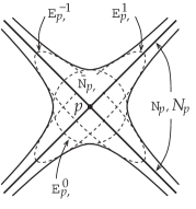
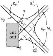
Figure 1: The structure of $\bar{\mathcal{N}}_{p,\epsilon}$ in Minkowski spacetime $\mathbb{M}$. Three of the ellipsoidal sets $\mathcal{E}_{p,\epsilon}^{\,\xi}$ are displayed, for $\xi=-1$,$0$ and $1$. To the right a subset of $\mathbb{M}$ is cut out, showing how the extension of a null geodesic which was originally passing through a boundary point of the cut out set is recovered in $\mathcal{N}_{p}$.

To illustrate the importance of $\mathcal{U}$ being compact in Theorem 5.5, we consider a modification of Minkowski spacetime by cutting out points. If a point $q$ on one of the null geodesics from a point $p$ is cut out, the light cone $N_{p}$ will not contain the part of the null geodesic after the missing point. But it will be contained in $\mathcal{N}_{p}$, provided that not too many points are missing around $q$ (see Figure 1).

6.2 Misner spacetime

Since the conditions of Theorem 5.5 exclude the case when $\mathcal{U}$ contains imprisoned null geodesics, it is interesting to study an example when this is the case. We choose the Misner spacetime [8, 5, 4], as it is a simple example with imprisoned curves.

Misner spacetime may be obtained from Minkowski spacetime $\mathbb{M}$ by identification under the isometry group generated by a fixed Lorentz boost $L_{0}$. For simplicity, we restrict attention to two dimensions. Let $L_{0}$ be given by

$$L_{0}\colon(t,x)\mapsto(t\cosh\xi_{0}+x\sinh\xi_{0},t\sinh\xi_{0}+x\cosh\xi_{0}),$$ (41)

and identify points on $\mathbb{M}_{+}:=\{(t,x);\;t+x>0\}$ under the discrete isometry group $\mathcal{G}$ generated by $L_{0}$. We then obtain a spacetime with topology $\mathbb{R}\times\mathbb{S}$. If we introduce new coordinates (c.f. [5])

$$\tau:=\tfrac{1}{4}(t^{2}-x^{2})\qquad\text{and}\qquad\psi:=\ln(t+x)^{2}-\ln 4,$$ (42)

with $\tau\in\mathbb{R}$ and $\psi\in[0,2\pi]$, the Minkowski metric transforms to

$$\mathrm{d}s^{2}=2\,\mathrm{d}\tau\,\mathrm{d}\psi+\tau\,\mathrm{d}\psi^{2}.$$ (43)

The null geodesics of $M$ can be divided into three families (see Figure 2):

1. Null geodesics obtained from the null geodesics with constant $t+x$ in $\mathbb{M}_{+}$. Being given by constant $\psi$, they are complete and pass through $\tau=0$.

2. Null geodesics obtained from the null geodesics with constant $t-x$ in $\mathbb{M}_{+}$. They are incomplete and endless, spiralling around the spacetime indefinitely as $\tau\to 0$. Hence they are totally imprisoned in any neighbourhood of $\tau=0$.

3. The closed null geodesic at $\tau=0$, which is incomplete and endless.

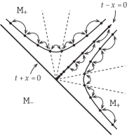
Identify under $\mathcal{G}$

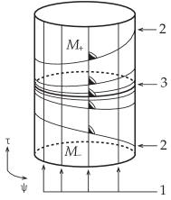
Figure 2: Two-dimensional Misner spacetime. Points in $\mathbb{M}_{+}$ are identified under the discrete isometry group $\mathcal{G}$. The arrows in the left figure show the identification of points on orbits of $\mathcal{G}$. The figure on the right shows the three families of null geodesics: family 1 obtained from null geodesics in $\mathbb{M}_{+}$ with constant $t+x$, family 2 obtained from null geodesics with constant nonvanishing $t-x$, and family 3 consisting of the single null geodesic corresponding to $t-x=0$.

The structure of $\mathcal{N}_{p}$ for Misner spacetime may be deduced from our knowledge of the Minkowski case. Let $M_{+}$ be the part of $M$ where $\tau>0$, and suppose that $p\in M_{+}$. Also, let $L$ be a Lorentz boost with hyperbolic angle $\xi$. We may identify $M_{+}$ with the wedge

$$\mathcal{W}:=\{(t,x)\in\mathbb{M};\;\lvert x/t\rvert<\tanh(\xi_{0}/2),\,t>0\}$$ (44)

(see Figure 3). Let $\tilde{p}$ be the point in $\mathcal{W}$ corresponding to $p$, let $\gamma$ be a null geodesic through $p$, and let $\tilde{\gamma}$ be the corresponding null geodesic segments in $\mathcal{W}$ as in Figure 3. Clearly, the ellipsoidal neighbourhood $\mathcal{E}_{p,\epsilon}^{\,\xi}$ of $p$ in $\mathbb{M}$ corresponds to a neighbourhood of $\tilde{\gamma}$. It follows that $\mathcal{N}_{p}(M_{+})=N_{p}(M_{+})$. By a similar argument, the same holds for the part of $M$ with $\tau<0$.

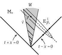
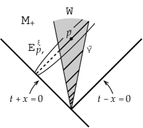
Figure 3: A neighbourhood $\mathcal{E}_{p,\epsilon}^{\,\xi}$ in two-dimensional Misner spacetime. In the left figure, a part of a null geodesic of family 1 is shown. For sufficiently large negative $\xi$, no points on the intersection of $\mathcal{E}_{p,\epsilon}^{\,\xi}$ with $t-x=0$ are identified under $\mathcal{G}$. On the right, it is shown how the past part of a null geodesic of family 2 is contained in $\mathcal{E}_{p,\epsilon}^{\,\xi}$ for large enough $\xi$.

We now include the set $\tau=0$. We have two cases. Suppose that $\gamma$ belongs to family 2, i.e., the extension of $\tilde{\gamma}$ passes through the line $t-x=0$ in $\mathbb{M}$. As $\xi\to-\infty$, the intersection of $\mathcal{E}_{p,\epsilon}^{\,\xi}$ with $t-x=0$ tends to the intersection point of $\tilde{\gamma}$ with $t-x=0$, which of course corresponds to the intersection of $\gamma$ with $\tau=0$.

On the other hand, suppose that $\gamma$ belongs to family 1, i.e., the extension of the part of $\tilde{\gamma}$ through $p$ hits the line $t+x=0$ in $\mathbb{M}$. Let $\gamma^{\prime}$ be a null geodesic parallel to $\gamma$, with image $\tilde{\gamma}^{\prime}$ in $\mathcal{W}$, such that $\tilde{\gamma}$ and $\tilde{\gamma}^{\prime}$ are different null geodesics in $M$. For large enough $\xi_{0}$, $\mathcal{E}_{p,\epsilon}^{\,\xi}$ does not intersect the extensions of the two segments of $\tilde{\gamma}^{\prime}$ closest to $p$. Since the isometry group is properly discontinuous, the same holds for the image of $\mathcal{E}_{p,\epsilon}^{\,\xi}$ and $\gamma^{\prime}$ in $M$. Hence no horizontal curve of sufficiently short b-length will reach $\tau=0$ in this direction, so the only points of $\mathcal{N}_{p}$ obtained in this way is the null geodesic $\gamma$ itself.

It remains to consider points $p$ lying on the closed null geodesic at $\tau=0$. Suppose that there is a point $q\in\mathcal{N}_{p}$ which does not lie on $\tau=0$. Then $p\in\mathcal{N}_{q}$, and we showed above that $\mathcal{N}_{q}=N_{q}$ if $\tau\neq 0$ at $q$. So there is a null geodesic from $q$ to $p$. We conclude that $\mathcal{N}_{p}=N_{p}$ for Misner spacetime.

6.3 Robertson-Walker spacetimes

Of course, Misner spacetime might be uninteresting from a cosmological point of view, partly because it is flat, and partly because some cosmologists argue that there are no signs of topological pathologies in the real universe. It is therefore important to obtain some results for more realistic cosmological models. Some of the simplest are the Robertson-Walker models, with topology $M=I\times\Sigma$ where $I$ is a real interval, and line element

$$\mathrm{d}s^{2}=-\mathrm{d}t^{2}+a(t)^{2}\mathrm{d}\sigma^{2},$$ (45)

such that $(\Sigma,\mathrm{d}\sigma^{2})$ is a homogeneous space (see, e.g., [5, 9]). The scale function $a(t)$ is determined from the chosen matter model via Einstein’s field equations. For a Friedman big bang model, $a(t)\to 0$ as $t\to 0$, corresponding to a curvature singularity at $t=0$.

It can be shown that the b-boundary $\partial_{b}M$ is a single point [2, 15, 1, 6]. Hence all null geodesics end at the same boundary point, and since the b-length of a null geodesic can be made arbitrarily small by an appropriate boost of the frame, the boundary point is not Hausdorff separated from any interior point of $M$. Moreover, the boundary fibre in $OM$ is completely degenerate so the boundary of $OM$ is a single point as well. This means that, along a curve ending at the singularity, choosing a different frame makes no difference at the boundary. It would therefore seem like $\mathcal{N}_{p}$ should be the whole spacetime $M$. But this is not necessarily the case, since the boundary point in $OM$ is singular with respect to the geometry in $OM$ as well, the curvature scalar tending to $-\infty$ at the boundary [16].

We will try to obtain an estimate of the neighbourhoods $\mathcal{E}_{p,\epsilon}^{\,\xi}$ for a particular Robertson-Walker model, valid for sufficiently small $\epsilon$. However, we should mention from the outset that the estimates break down when $\mathcal{E}_{p,\epsilon}^{\,\xi}$ intersects the singularity. This is unfortunate because the structure near the singularity is exactly what might cause identifications, giving a nontrivial $\mathcal{N}_{p}$. The problem is the usual one when working with b-length: the length functional is not additive, in the sense that the length on a segment of the curve depends on the frame, which in turn is determined by parallel propagation along the whole curve. Also, the situation is not as simple as in Minkowski or Misner space, since the b-extremal curves are likely to develop ‘conjugate points’.

We will restrict attention to a two-dimensional model for simplicity. This is in fact not a restriction since $(\Sigma,\mathrm{d}\sigma^{2})$ is homogeneous. Let the metric be given by

$$\mathrm{d}s^{2}=-\mathrm{d}\bar{t}^{2}+a(\bar{t})^{2}\,\mathrm{d}x^{2}.$$ (46)

We will fix the scale factor $a(\bar{t})$ later. If we replace the coordinate $\bar{t}$ with a conformal coordinate $t:=\int a^{-1}\mathrm{d}t$ and redefine the scale factor as a function $a(t)$ of $t$, the metric takes the form

$$\mathrm{d}s^{2}=a(t)^{2}(-\mathrm{d}t^{2}+\mathrm{d}x^{2}).$$ (47)

Any pseudo-orthonormal frame over $M$ may be expressed as $E\mathbf{L}(\xi)$, where $E$ is the global frame field given by $(a^{-1}\frac{\partial}{\partial t},a^{-1}\frac{\partial}{\partial x})$ and $\mathbf{L}(\xi)$ is a boost in the $t+x$ direction, i.e.,

$$E\mathbf{L}(\xi)=(\cosh\xi\,E_{0}+\sinh\xi\,E_{1},\sinh\xi\,E_{0}+\cosh\xi\,E_{1}).$$ (48)

Let $\gamma$ be a horizontal curve given by $(t(s),x(s),\xi(s))$. The equation for parallel propagation of $\xi$ along $\gamma$ is

$$\dot{\xi}+a^{\prime}a^{-1}\dot{x}=0,$$ (49)

where $a^{\prime}$ denotes the derivative of $a$ with respect to $t$. Expressing the tangent of $\gamma$ in the parallel frame $E\mathbf{L}(\xi)$ and inserting into the b-length formula (6) gives

$$l(\gamma)=\int a\bigl{(}\dot{t}^{2}\cosh 2\xi-2\,\dot{t}\dot{x}\sinh 2\xi+\dot{x}^{2}\cosh 2\xi\bigr{)}^{1/2}\,\mathrm{d}s.$$ (50)

If we parameterise $\gamma$ by b-length $s$, we get

$$\dot{t}^{2}\cosh 2\xi-2\,\dot{t}\dot{x}\sinh 2\xi+\dot{x}^{2}\cosh 2\xi=a^{-2}.$$ (51)

Now we assume that $\gamma$ is an extremal curve with respect to b-length. Since the integrand of (50) is functionally independent of $x$, the functional derivative with respect to $\dot{x}$ gives a first integral

$$\dot{x}\cosh 2\xi-\dot{t}\sinh 2\xi=\tfrac{1}{2}a^{-2}A,$$ (52)

where $A$ is a constant determined by the initial values at $s=0$. It is convenient to introduce an angular parameterisation of the initial values. First, we define null coordinates on $M$ by

$$u:=t+x\qquad\text{and}\qquad v:=t-x.$$ (53)

Then we may parameterise the initial conditions as

$$\dot{u}_{0}:=\sqrt{2}\,a_{0}^{-1}e^{\xi_{0}}\cos\theta\qquad\text{and}\qquad\dot{v}_{0}:=\sqrt{2}\,a_{0}^{-1}e^{-\xi_{0}}\sin\theta,$$ (54)

where $\theta\in[0,2\pi)$ is a constant and $a_{0}:=a(t_{0})$. With this parameterisation $A$ is

$$A=\sqrt{2}\,a_{0}(e^{-\xi_{0}}\cos\theta-e^{\xi_{0}}\sin\theta).$$ (55)

The three equations (49), (51) and (52) are sufficient for determining $\gamma$, given initial values for $t$, $x$, $\xi$ and $\theta$. It is possible to solve (52) for $\dot{x}$, and inserting the solution into (51) we may solve for $\dot{t}^{2}$. Put

$$W:=a^{2}\cosh 2\xi.$$ (56)

Then (49), (51) and (52) are equivalent to the system

$$\dot{t}^{2} =\tfrac{1}{4}\,a^{-4}\,(4W-A^{2})$$ (57)

$$\dot{x} =\frac{A}{2W}+\dot{t}\tanh 2\xi$$ (58)

$$\dot{\xi} =-a^{\prime}a^{-1}\dot{x}.$$ (59)

For simplicity, we now restrict ourselves to the case when the scale factor is $a(\bar{t})=\bar{t}^{1/2}$ (corresponding to a radiation-dominated universe), which will give us an idea about what to expect in general. In the conformal coordinate $t$, $a(t)=t/2$ and $a^{\prime}(t)=1/2$. We are now ready to state the result.

Proposition 6.1.

Let $(M,g)$ be a two-dimensional Robertson-Walker spacetime with scale factor $a(\bar{t})=\bar{t}^{1/2}$. Let $\gamma$ be a curve of extremal b-length, parameterised by b-length $s$ and starting at $(t_{0},x_{0},\xi_{0})$. Also, let $u=t+x$ and $v=t-x$. Suppose that $t<2t_{0}$ on $\gamma$. If $\xi_{0}>2$ then

$$\lvert v-v_{0}\rvert<16\,a_{0}^{-1}e^{-\xi}s$$

along $\gamma$. On the other hand, if $\xi_{0}<-2$ then

$$\lvert u-u_{0}\rvert<16\,a_{0}^{-1}e^{\xi}s.$$

Proof.

We start by estimating $W$, given by (56). Let $s_{1}$ be the largest number such that $W$ satisfies

$$\frac{1}{2}<\frac{W}{W_{0}}<2$$ (60)

on $[0,s_{1})$. Here $W_{0}$ is the value of $W$ at $s=0$. We show that either $t=0$ or $t=2t_{0}$ at $s=s_{1}$.

If we insert $a(t)=t/2$ in (57), we get

$$\lvert t^{2}\dot{t}\rvert=2\sqrt{4W-A^{2}}\leq 2\sqrt{4W}$$ (61)

on $[0,s_{1})$. Using (60) and integrating then gives

$$\lvert t^{3}-t_{0}^{3}\rvert<6\sqrt{8W_{0}}\,s.$$ (62)

Next, from (57–59) we have

$$\frac{\mathrm{d}}{\mathrm{d}s}\sqrt{W^{2}-a^{4}}=-a^{\prime}a^{-1}\!A=-t^{-1}\!A.$$ (63)

Using (62) and integrating gives

$$\Bigl{\lvert}\sqrt{W^{2}-a^{4}}-\sqrt{\smash[b]{W_{0}^{2}-a_{0}^{4}}}\Bigr{\rvert}<\frac{\lvert A\rvert}{4\sqrt{8W_{0}}}\Bigl{(}t_{0}^{2}-\bigl{(}t_{0}^{3}-6\sqrt{8W_{0}}\,s\bigr{)}^{2/3}\Bigr{)}<\frac{\lvert A\rvert}{4\sqrt{8W_{0}}}\,t_{0}^{2}.$$ (64)

Combining (56) and (55), we find that

$$4W_{0}-A^{2}\geq 0,$$ (65)

so the right hand side of (64) is less than $t_{0}^{2}/5$. Solving (64) for $W^{2}$ and dividing by $W_{0}^{2}$ we get

$$\frac{W^{2}}{W_{0}^{2}}<\frac{a^{4}}{W_{0}^{2}}+\biggl{(}\frac{\sqrt{\smash[b]{W_{0}^{2}-a_{0}^{4}}}}{W_{0}}+\frac{t_{0}^{2}}{5W_{0}}\biggr{)}^{2}.$$ (66)

Since $t<2t_{0}$ and $\lvert\xi_{0}\rvert>2$,

$$\frac{W}{W_{0}}<1.1<2.$$ (67)

Going back to (64) and estimating from below results in

$$\frac{W^{2}}{W_{0}^{2}}>\frac{a^{4}}{W_{0}^{2}}+\biggl{(}\frac{\sqrt{\smash[b]{W_{0}^{2}-a_{0}^{4}}}}{W_{0}}-\frac{t_{0}^{2}}{5W_{0}}\biggr{)}^{2}.$$ (68)

The first term is positive, and expanding the square and applying the conditions on $t$ and $\xi_{0}$ gives

$$\frac{W}{W_{0}}>0.98>\frac{1}{2}.$$ (69)

From (67) and (69) it follows that (60) cannot be violated even at $s=s_{1}$. So unless $t(s_{1})=0$, the only remaining possibility is that $t(s_{1})=2t_{0}$.

The next step is to estimate $\xi$ in terms of $\xi_{0}$. Using the definition (56) of $W$ and the lower bound of (60) gives

$$e^{2\lvert\xi\rvert}>\cosh 2\xi>\frac{t_{0}^{2}}{2t^{2}}\cosh 2\xi_{0}>\frac{1}{16}\,e^{2\lvert\xi_{0}\rvert},$$ (70)

hence

$$\lvert\xi\rvert>\lvert\xi_{0}\rvert-\ln 4.$$ (71)

We can now provide bounds for $\dot{u}=\dot{t}+\dot{x}$ and $\dot{v}=\dot{t}-\dot{x}$. Suppose that $\xi_{0}>2$. From (57) and (58),

$$\lvert\dot{v}\rvert=\biggl{\lvert}(1+\tanh 2\xi)\,\dot{t}+\frac{A}{2W}\biggr{\rvert}<W^{-1/2}(e^{2\xi}+\sqrt{2}),$$ (72)

where the inequality follows from (65) and (60). But

$$W^{-1/2}(e^{2\xi}+\sqrt{2})<2\sqrt{2}\,a_{0}^{-1}e^{-\xi}\frac{\cosh\xi}{\sqrt{\cosh 2\xi}}<2\sqrt{2}\,a_{0}^{-1}e^{-\xi},$$ (73)

so using (71) and integrating gives the desired bound on $\lvert v-v_{0}\rvert$. The argument for the case when $\xi_{0}<-2$ is similar. ∎

The problem when trying to use Proposition 6.1 to estimate the extent of $\mathcal{E}_{p,\epsilon}^{\,\xi}$ is that while we have valid estimates for curves ‘near’ $p$, it is likely that curves that approach $t=0$ will no longer have minimal b-length. In a sense, there will be ‘conjugate points’ with respect to the b-length. Is it possible to find arbitrarily short curves between two distinct null geodesics? It seems unlikely since boosting the frame in order to get close to the singularity will probably make it impossible to move a finite distance in the $x$-direction without spending too much b-length. We therefore make the following conjecture.

Conjecture 6.2.

In a Robertson-Walker spacetime, with a ‘physically reasonable’ equation of state, $\mathcal{N}_{p}=N_{p}$.

7 Imprisonment and fibre degeneracy

Let $\gamma:(0,1]\to OM$ be a horizontal curve with $\gamma(t)\to E\in\partial OM$ as $t\to 0$. In [15] it was shown that if there are sequences $t_{i}\to 0$ and $\rho_{i}\to 0$ of real numbers such that the following conditions hold, the boundary fibre containing $E$ is totally degenerate:

1. the closure of each ball $\mathcal{U}_{i}:=B_{\rho_{i}}(\gamma(t_{i}))$ in $\hskip 1.79993pt\overline{OM}$ is compact and contained in $OM$.

2. $\mathbf{R}$, the frame components of Riemann tensor viewed as a map from the space of bivectors to the Lie algebra, is invertible on each $\mathcal{U}_{i}$.

3. $\lVert{\mathbf{R}(\gamma(t_{i}))^{-1}}\rVert^{3}\sup_{\mathcal{U}_{i}}\lVert{\mathbf{R}}\rVert^{2}$, $\lVert{\mathbf{R}(\gamma(t_{i}))^{-1}}\rVert^{2}\sup_{\mathcal{U}_{i}}\lVert{\mathbf{\nabla_{R}}}\rVert$ and $\lVert{\mathbf{R}(\gamma(t_{i}))^{-1}}\rVert/\!\rho_{i}$ all tend to $0$ as $t_{i}\to 0$. Here $\lVert{\cdot}\rVert$ is the mapping norm with respect to the frame in $OM$ and a fixed basis in the Lie algebra, respectively.

An explanation of condition 2 is given in Appendix B. We will now investigate if condition 3 is applicable to boundary points arising from imprisoned curves.

Suppose that an incomplete endless curve $\gamma$ is (partially or totally) imprisoned in a compact set $\mathcal{K}$. If the spacetime is sufficiently general, in particular, if it is of Petrov type I, some component of the Riemann tensor diverges in a parallel frame along $\gamma$ (see [5], Proposition 8.5.2). For condition 3 to hold, it is necessary that $\lVert{\mathbf{R}^{-1}}\rVert\to 0$, which is true if and only if $\lVert{\mathbf{R}(\mathbf{B})}\rVert\to\infty$ for all bivectors $\mathbf{B}$ with $\lVert{\mathbf{B}}\rVert=1$ [15]. So several components of $\mathbf{R}$ have to diverge in a specific manner.

Let $p\in\mathcal{K}$ be a cluster point of $\gamma$, let $\mathcal{U}$ be a convex normal neighbourhood around $p$ and let $\sigma$ be a section over $\overline{\mathcal{U}}$. Then $\lVert{\mathbf{R}}\rVert$ is bounded on $\sigma(\mathcal{U})$ since $\sigma(\mathcal{U})$ is contained in a compact set. It is clear from the proof of Lemma 4.1 that a diverging $\mathbf{R}$ can only be caused by a diverging Lorentz transformation along $\gamma$.

Since $\lVert{\mathbf{R}^{-1}}\rVert$ is unaffected by spatial rotations, we only need to study the effect of a boost. Fix a frame $E$ at a point $q\in\mathcal{U}$ and put $E_{u}:=(1/\sqrt{2})(E_{0}+E_{1})$ and $E_{v}:=(1/\sqrt{2})(E_{0}-E_{1})$. Let $\mathbf{L}$ be a boost by an hyperbolic angle $\xi$ in the $E_{u}$ direction, as given by equation (32), and let $\mathbf{B}=E_{u}\wedge E_{2}$. Then if $\mathbf{R}$ is the Riemann tensor expressed in the boosted frame $E\mathbf{L}$ and $R^{i}\!_{jkl}$ are the components of the Riemann tensor in the fixed frame $E$,

$$\lVert{\mathbf{R}(\mathbf{B})}\rVert^{2}=(R^{u}\!_{2u2})^{2}+(R^{u}\!_{3u2})^{2}+o(e^{-2\xi}),$$ (74)

where $o(e^{-2\xi})$ denotes terms less than a constant times $e^{-2\xi}$ for $\xi$ sufficiently large. So there is a bivector $\mathbf{B}$ such that $\mathbf{R}(\mathbf{B})$ is bounded away from 0, which implies that $\lVert{\mathbf{R}^{-1}}\rVert\not\to 0$. We conclude that condition 3 does not hold for points in $\partial OM$ arising from imprisoned curves. Note that even though the techniques in [15] do not apply, the boundary fibre might still be partially or totally degenerate.

8 Discussion

It seems likely that the compactness and non-imprisonedness conditions in Theorem 5.5 may be removed, at least in some cases. A first step would be to extend Proposition 6.1 to cover more general Robertson-Walker spacetimes, and perhaps to other cosmological models. That would give a better handle on b-boundary issues in more realistic cosmologies. Also, in Schwarzschild spacetime it is still unknown if the b-boundary is a set of dimension 0 or 1. Hopefully, the techniques used in section 6.3 can be generalised to cover a two-dimensional version of the Schwarzschild spacetime as well, since in two dimensions the inner part (i.e., inside the event horizon) can be written in the Robertson-Walker form (46) for a particular choice of scale factor $a(\bar{t})$.

It would also be interesting to obtain a fibre degeneracy theorem, similar to the one in [15], that is applicable to the imprisoned curve setting. It seems probable that only partial degeneracy can be expected in this case. However, very different techniques will be needed than those used in [15].

Appendix A Horizontal curves

When working in the pseudo-orthonormal frame bundle $OM$ it is often convenient to restrict attention to horizontal curves. A statement of the following form can be found in the literature (cf. [3], p. 442 and [2], pp. 36–38).

Claim.

Let $\tilde{\lambda}\colon[0,a)\to OM$ be a finite curve and let $\bar{\lambda}$ be the horizontal lift of $\pi\circ\tilde{\lambda}$ with $\bar{\lambda}(0)=\tilde{\lambda}(0)$. Then

$$l(\bar{\lambda})\leq l(\tilde{\lambda}).$$ (75)

However, this statement is generally false, as we will now see. Given $\tilde{\lambda}$ and $\bar{\lambda}$ as above, there is a curve $\mathbf{L}$ in $\mathcal{L}$ such that $\tilde{\lambda}(t)=\bar{\lambda}(t)\mathbf{L}(t)$ for all $t\in[0,a)$, with $\mathbf{L}(0)=\delta$, the identity in $\mathcal{L}$. Then

$$\dot{\tilde{\lambda}}(t)=R_{\mathbf{L}(t)*}(\dot{\bar{\lambda}}(t))+\frac{\mathrm{d}}{\mathrm{d}s}\Bigr{|}_{s=t}\bigl{(}R_{\mathbf{L}(s)}(\bar{\lambda}(t))\bigr{)}=R_{\mathbf{L}(t)*}(\dot{\bar{\lambda}}(t))+\varphi(\mathbf{L}^{-1}\dot{\mathbf{L}}),$$ (76)

where $\varphi$ is the canonical isomorphism from the Lie algebra $\mathfrak{l}$ to the vertical subspace $V(OM)$ of  $T(OM)$ at $\tilde{\lambda}(t)$ [7]. Now

$$\boldsymbol{\theta}(\dot{\tilde{\lambda}})=\boldsymbol{\theta}(R_{\mathbf{L}*}\dot{\bar{\lambda}})=\mathbf{L}^{-1}\boldsymbol{\theta}(\dot{\bar{\lambda}})$$ (77)

because of the transformation properties of the canonical 1-form $\boldsymbol{\theta}$ under the right action of $\mathcal{L}$ [7]. Also

$$\boldsymbol{\omega}(\dot{\tilde{\lambda}})=\varphi^{-1}(\operatorname{ver}\dot{\tilde{\lambda}})=\mathbf{L}^{-1}\dot{\mathbf{L}},$$ (78)

where $\operatorname{ver}\dot{\tilde{\lambda}}$ is the vertical component of $\dot{\tilde{\lambda}}$ [7]. We conclude that

$$l(\tilde{\lambda})=\int_{0}^{a}\Bigl{(}\lVert{\mathbf{L}^{-1}\boldsymbol{\theta}(\dot{\bar{\lambda}})}\rVert^{2}+\lVert{\mathbf{L}^{-1}\dot{\mathbf{L}}}\rVert^{2}\Bigr{)}^{1/2}\,\mathrm{d}t.$$ (79)

It seems that the mistakes in [2] and [3] stem from neglecting the $\mathbf{L}^{-1}$ factor, which originates from the b-norm being evaluated at different points in the fibre over $\pi\circ\tilde{\lambda}(t)$.

As an example, consider a null geodesic $\gamma$ with horizontal lift $\bar{\gamma}$, affinely parameterised by $t\in[0,a)$. Let $\tilde{\gamma}$ be the curve given by $\tilde{\gamma}(t)=\bar{\gamma}(t)\mathbf{L}(t)$ where $\mathbf{L}(t)$ is a Lorentz boost in the direction of $\dot{\gamma}$ by an hyperbolic angle $\xi(t)$ with $\xi(0)=0$. Then

$$l(\tilde{\gamma})=\int_{0}^{a}\Bigl{(}2\dot{\xi}(t)^{2}+e^{-2\xi(t)}\Bigr{)}^{1/2}\,\mathrm{d}t,$$ (80)

which certainly can be made smaller than $l(\bar{\gamma})=a$ by an appropriate choice of $\xi(t)$.

However, note that in the frame bundle of a Riemannian manifold,

$$\lVert{\mathbf{L}^{-1}\boldsymbol{\theta}(\dot{\bar{\lambda}})}\rVert=\lvert\boldsymbol{\theta}(\dot{\bar{\lambda}})\rvert$$ (81)

since in that case $\mathbf{L}\in O(4)$, the orthogonal transformation group. It follows that (79) reduces to

$$l(\tilde{\lambda})=\int_{0}^{a}\Bigl{(}\lvert\boldsymbol{\theta}(\dot{\bar{\lambda}})\rvert^{2}+\lVert{\mathbf{L}^{-1}\dot{\mathbf{L}}}\rVert^{2}\Bigr{)}^{1/2}\,\mathrm{d}t\leq\int_{0}^{a}\lvert\boldsymbol{\theta}(\dot{\bar{\lambda}})\rvert\,\mathrm{d}t=l(\bar{\lambda}).$$ (82)

This result was used by Schmidt [12] in proving that the b-completion is equivalent to the Cauchy completion in the Riemannian case.

In the Lorentzian case, it is still possible to find a connection between the lengths of horizontal curves and more general curves, being almost as strong as the relation (75) for short curves.

Proposition A.1.

Let $\tilde{\lambda}:[0,a)\to OM$ be a curve with finite b-length, and let $\bar{\lambda}$ be the horizontal lift of $\pi\circ\tilde{\lambda}$ with $\bar{\lambda}(0)=\tilde{\lambda}(0)$. Then

$$l(\bar{\lambda})\leq e^{l(\tilde{\lambda})}-1.$$ (83)

Proof.

We may assume that $\tilde{\lambda}$ is parameterised by b-length and that $\tilde{\lambda}(t)=\bar{\lambda}(t)\mathbf{L}(t)$ for some curve $\mathbf{L}$ in $\mathcal{L}$, with $\mathbf{L}(0)=\delta$. Then by (79),

$$\lvert\dot{\tilde{\lambda}}\rvert^{2}=\lvert\boldsymbol{\theta}(\dot{\tilde{\lambda}})\rvert^{2}+\lVert{\mathbf{L}^{-1}\dot{\mathbf{L}}}\rVert^{2}=1,$$ (84)

so $\lvert\boldsymbol{\theta}(\dot{\tilde{\lambda}})\rvert\leq 1$. Since $\mathbf{L}(t)$ is a curve in $\mathcal{L}$, there is a curve $\mu$ in the Lie algebra $\mathfrak{l}$ such that $\mathbf{L}(t)=\exp\mu(t)$, where $\exp$ is the exponential map $\mathfrak{l}\to\mathcal{L}$ and $\mu(0)=0$. Then by (84), $\lvert\dot{\mu}\rvert=\lVert{\mathbf{L}^{-1}\dot{\mathbf{L}}}\rVert\leq 1$. It follows that

$$\frac{\mathrm{d}}{\mathrm{d}t}\lvert\mu\rvert\leq\lvert\dot{\mu}\rvert\leq 1,$$ (85)

which on integration gives $\lvert\mu\rvert\leq t$. Thus

$$\lVert{\mathbf{L}}\rVert\leq\lvert\exp\mu\rvert\leq e^{\lvert\mu\rvert}\leq e^{t},$$ (86)

so using (77) gives

$$l(\bar{\lambda})=\int_{0}^{a}\lvert\mathbf{L}\boldsymbol{\theta}(\dot{\tilde{\lambda}})\rvert\,\mathrm{d}t\leq\int_{0}^{a}e^{t}\,\mathrm{d}t=e^{a}-1.$$ (87)

∎

Proposition A.1 then reestablishes the result in section 3.13 of [3], p. 441, and the crucial steps in the proof of Proposition 3.2.1 of [2], p. 38.

Appendix B Invertibility of the Riemann tensor

This section serves to clarify the invertibility condition on the Riemann tensor in a given frame, viewed as a linear map from the space of bivectors to the Lie algebra of the Lorentz group. Clearly, if $\mathbf{R}$ is invertible in one frame at a point $p\in M$, it is invertible in any other frame at $p$. We restrict attention to the vacuum case when $\mathbf{R}=\mathbf{C}$, the Weyl tensor, for simplicity. We will investigate the relation between invertibility of $\mathbf{C}$ and Petrov types, so we use a spinor formalism (see, e.g., [10] and [17]). This requires a change of signature of the metric, which has no influence on the invertibility. Also, we may study $\mathbf{C}_{abcd}=\eta_{ae}\mathbf{C}^{e}\!_{bcd}$ instead of $\mathbf{C}^{a}\!_{bcd}$. In spinor form, we have

$$\mathbf{C}_{abcd}=\mathbf{C}_{ABCDA^{\prime}B^{\prime}C^{\prime}D^{\prime}}=\Psi_{\!ABCD}\,\epsilon_{\!A^{\prime}B^{\prime}}\,\epsilon_{C^{\prime}D^{\prime}}+\bar{\Psi}_{\!A^{\prime}B^{\prime}C^{\prime}D^{\prime}}\,\epsilon_{\!AB}\,\epsilon_{CD},$$ (88)

where $\Psi_{\!ABCD}$ is the symmetric Weyl spinor. Any bivector $\mathbf{B}^{cd}$ may be decomposed as

$$\mathbf{B}^{cd}=\mathbf{B}^{CDC^{\prime}D^{\prime}}=\phi^{CD}\epsilon^{C^{\prime}D^{\prime}}+\bar{\phi}^{\,C^{\prime}D^{\prime}}\epsilon^{CD}$$ (89)

where $\phi^{CD}$ is a symmetric spinor. Let $\mathcal{S}^{2}$ be the space of symmetric contravariant valence 2 spinors, and let $\mathcal{S}^{2*}$ be the dual space of $\mathcal{S}^{2}$. It is easily found that $\mathbf{C}_{abcd}\mathbf{B}^{cd}=0$ for some bivector $\mathbf{B}^{cd}$ if and only if $\Psi_{\!ABCD}\,\phi^{CD}=0$ for some $\phi^{CD}\in\mathcal{S}^{2}$. So $\mathbf{C}$ is invertible if and only if $\Psi\colon\mathcal{S}^{2}\to\mathcal{S}^{2*}$ is invertible.

Given a spin basis $o^{A},\iota^{A}$, we define a basis for $\mathcal{S}^{2}$ by

$$E_{1}^{AB}=o^{A}o^{B},\qquad E_{2}^{AB}=o^{(A}\iota^{B)}\qquad\text{and}\qquad E_{3}^{AB}=\iota^{A}\iota^{B}.$$ (90)

Then the corresponding dual basis for $\mathcal{S}^{2*}$ is

$$E^{1}_{AB}=\iota_{\!A}\iota_{B},\qquad E^{2}_{AB}=-o_{(A}\iota_{B)}\qquad\text{and}\qquad E^{3}_{AB}=o_{\!A}o_{B}.$$ (91)

In this basis, $\Psi:\mathcal{S}^{2}\to\mathcal{S}^{2}$ may be written as

$$\Psi=\begin{bmatrix}\Psi_{0}&\Psi_{1}&\Psi_{2}\\ \Psi_{1}&\Psi_{2}&\Psi_{3}\\ \Psi_{2}&\Psi_{3}&\Psi_{4}\end{bmatrix}.$$ (92)

Thus the determinant $\det{\Psi}$ is one of the two independent curvature scalars that can be constructed from the Weyl tensor. Since the invertibility of $\Psi$ is independent of the choice of spin basis, we can choose $o^{A}$ as one of the principal null directions of $\Psi_{\!ABCD}$. Then $\Psi_{0}=0$, and the determinant of $\Psi$ becomes

$$\det{\Psi}=-\Psi_{2}^{3}+2\,\Psi_{1}\Psi_{2}\Psi_{3}-\Psi_{1}^{2}\Psi_{4}.$$ (93)

Now if the Weyl tensor is of type III, N or O, three principal spinors of $\Psi$ coincide. If we choose this repeated spinor as $o^{A}$, $\Psi_{1}=\Psi_{2}=0$, so $\Psi$ is singular. On the other hand, if only two principal spinors coincide, i.e., the Weyl tensor is of type II or D, $\Psi_{1}=0$ and $\Psi_{2}\neq 0$ so $\Psi$ is invertible.

It remains to study the most general case with no repeated principal spinors (Petrov type I). We may choose $o^{A}$ and $\iota^{A}$ as two of the four principal spinors. Then $\Psi_{0}=\Psi_{4}=0$, and we may write $\Psi_{\!ABCD}=o_{(A}\iota_{B}\alpha_{C}\beta_{D)}$ for two linearly independent spinors $\alpha_{\!A}$ and $\beta_{\!A}$. Let

$$\alpha_{\!A}=\alpha_{0}o_{\!A}+\alpha_{1}\iota_{\!A}\qquad\text{and}\qquad\beta_{\!A}=\beta_{0}o_{\!A}+\beta_{1}\iota_{\!A}.$$ (94)

Then

$$\Psi_{1}=-\tfrac{1}{4}\alpha_{1}\beta_{1},\quad\Psi_{2}=\tfrac{1}{6}(\alpha_{0}\beta_{1}+\alpha_{1}\beta_{0})\quad\text{and}\quad\Psi_{3}=-\tfrac{1}{4}\alpha_{0}\beta_{0}.$$ (95)

Now (93) is

$$\det{\Psi}=-\Psi_{2}(\Psi_{2}^{2}-2\,\Psi_{1}\Psi_{3}),$$ (96)

and the second factor is

$$-\tfrac{1}{288}(\alpha_{0}\beta_{1}+\alpha_{1}\beta_{0})^{2}+\tfrac{1}{32}(\alpha_{0}\beta_{1}-\alpha_{1}\beta_{0})^{2}.$$ (97)

So if $\Psi$ is singular, we must have

$$\alpha_{0}\beta_{1}=2\alpha_{1}\beta_{0}$$ (98)

up to an interchange of $\alpha$ and $\beta$. The algebraic condition (98) corresponds to two real equations, so it can be expected to hold on a subset of codimension two in $M$ for generic spacetimes. In particular, the solution set has empty interior.

References

- [1] B. Bosshard, On the b-boundary of the closed Friedman-model, Comm. Math. Phys. 46 (1976), 263–268.
- [2] C. J. S. Clarke, The analysis of space-time singularities, Cambridge University Press, Cambridge, 1993.
- [3] C. T. J. Dodson, Space-time edge geometry, Int. J. Theor. Phys. 17 (1978), no. 6, 389–504.
- [4] G. F. R. Ellis and B. G. Schmidt, Singular space-times, Gen. Rel. Grav. 8 (1977), no. 11, 915–953.
- [5] S. W. Hawking and G. F. R. Ellis, The large scale structure of space-time, Cambridge Univ. Press, Cambridge, 1973.
- [6] R. Johnson, The bundle boundary in some special cases, J. Math. Phys. 18 (1977), 898–902.
- [7] S. Kobayashi and K. Nomizu, Foundations of differential geometry, vol. I, John Wiley & Sons, New York, 1963.
- [8] C. W. Misner, Taub-NUT space as a counterexample to almost anything, Relativity Theory and Astrophysics: I. Relativity and Cosmology (J. Ehlers, ed.), Lectures in Applied Mathematics, vol. 8, Amer. Math. Soc., Providence, RI, 1967, pp. 160–169.
- [9] C. W. Misner, K. S. Thorne, and J. A. Wheeler, Gravitation, W. H. Freeman and Company, New York, 1973.
- [10] R. Penrose and W. Rindler, Spinors and space-time 1: Two-spinor calculus and relativistic fields, Cambridge University Press, Cambridge, 1984.
- [11] V. Perlick, Notes on variations of the b-length functional, personal communication.
- [12] B. G. Schmidt, A new definition of singular points in general relativity, Gen. Rel. Grav. 1 (1971), no. 3, 269–280.
- [13] , The local b-completeness of space-times, Comm. Math. Phys. 29 (1973), 49–54.
- [14] F. Ståhl, A local variational theory for the Schmidt metric, J. Math. Phys. 38 (1997), 3347–3357, gr-qc/9612005.
- [15] , Degeneracy of the b-boundary in general relativity, Comm. Math. Phys. 208 (1999), 331–353, gr-qc/9906021.
- [16] , The geometry of the frame bundle over spacetime, submitted to J. Math. Phys., 2000, gr-qc/0006049.
- [17] J. Stewart, Advanced general relativity, Cambridge University Press, Cambridge, 1990.
- [18] R. M. Wald, General relativity, University of Chicago Press, Chicago, 1984.