The Bianchi IX attractor

Abstract.

We consider the asymptotic behaviour of spatially homogeneous spacetimes of Bianchi type IX close to the singularity (we also consider some of the other Bianchi types, e. g. Bianchi VIII in the stiff fluid case). The matter content is assumed to be an orthogonal perfect fluid with linear equation of state and zero cosmological constant. In terms of the variables of Wainwright and Hsu, we have the following results. In the stiff fluid case, the solution converges to a point for all the Bianchi class A types. For the other matter models we consider, the Bianchi IX solutions generically converge to an attractor consisting of the closure of the vacuum type II orbits. Furthermore, we observe that for all the Bianchi class A spacetimes, except those of vacuum Taub type, a curvature invariant is unbounded in the incomplete directions of inextendible causal geodesics.

1. Introduction

The last few decades, the Bianchi IX spacetimes have received considerable attention, see for instance [5], [11], [18] and references therein. Agreement has been reached, at least concerning some aspects of the asymptotic behaviour as one approaches a singularity, but the basis for the consensus has mainly consisted of numerical studies and heuristic arguments. The objective of this article is to provide mathematical proofs for some aspects of the ’accepted’ picture. The main result of this paper was for example conjectured in [18] p. 146-147, partly on the basis of a numerical analysis.

Why Bianchi IX? One reason is the fact that this class contains the Taub-NUT spacetimes. These spacetimes are vacuum maximal globally hyperbolic spacetimes that are causally geodesically incomplete both to the future and to the past, see [6] and [14]. However, as one approaches a singularity, in the sense of causal geodesic incompleteness, the curvature remains bounded. In fact, one can extend the spacetime beyond the singularities in inequivalent ways, see [6]. It is natural to conjecture that the behaviour exhibited by the Taub-NUT spacetimes is non-generic, and it is interesting to try to prove that the behaviour is non-generic in the Bianchi IX class. In fact we prove that all Bianchi IX initial data considered in this paper other than Taub-NUT yield inextendible globally hyperbolic developments such that the curvature becomes unbounded as one approaches a singularity. This result is in fact more of an observation, since the corresponding result is known in the vacuum case, see [16], and curvature blow up is easy to prove in the non-vacuum cases we consider.

Another reason for studying the Bianchi IX spacetimes is the BKL conjecture, see [3]. According to this conjecture, the ’local’ approach to the singularity of a general solution should exhibit oscillatory behaviour. The prototypes for this behaviour among the spatially homogeneous spacetimes are the Bianchi VIII and IX classes. Furthermore the matter is conjectured to become unimportant as one approaches a singularity, with some exceptions, for example the stiff fluid case. We refer to [4] for arguments supporting the BKL conjecture and to [1] for an overview of conjectures and results under symmetry assumptions of varying degree. In this paper we prove, under certain restrictions on the allowed matter models, that generic Bianchi IX solutions exhibit oscillatory behaviour and that the matter becomes unimportant as one approaches a singularity. What is meant by the latter statement will be made precise below. If the matter model is a stiff fluid the matter will be important, and in that case we prove that the behaviour is quiescent. This should be compared with [2] concerning the structure of singularities of analytic solutions to Einstein’s equations coupled to a scalar field or stiff fluid. In that paper, Andersson and Rendall prove that given a certain kind of solution to the so called velocity dominated system, there is a unique solution of Einstein’s equations coupled to a stiff fluid approaching the velocity dominated solution asymptotically. One can then ask the question whether it is natural to assume that a solution has the asymptotics they prescribe. In Section 20, we show that all Bianchi VIII and IX stiff fluid solutions exhibit such asymptotic behaviour.

The results presented in this paper can be divided into two parts. The first part consists of statements about developments of orthogonal perfect fluid data of class A. We clarify below what we mean by this. The results concern curvature blow up and inextendibility of developments. The second part consists of results expressed in terms of the variables of Wainwright and Hsu. These variables describe the spacetime close to the singularity, and we prove that Bianchi IX solutions generically converge to a set on which the flow of the equation coincides with the Kasner map.

We consider spatially homogeneous Lorentz manifolds $(\bar{M},\bar{g})$ with a perfect fluid source. The stress energy tensor is thus given by

(1.1) $$T_{ab}=\mu u_{a}u_{b}+p(\bar{g}_{ab}+u_{a}u_{b}),$$

where $u$ is a unit timelike vectorfield, the 4-velocity of the fluid. We assume that $p$ and $\mu$ satisfy a linear equation of state

(1.2) $$p=(\gamma-1)\mu,$$

where we in this paper restrict our attention to $2/3<\gamma\leq 2$. We will also assume that $u$ is perpendicular to the hypersurfaces of homogeneity. Einstein’s equations can be written

(1.3) $$\bar{R}_{ab}-\frac{1}{2}\bar{R}\bar{g}_{ab}=T_{ab},$$

where $\bar{R}_{ab}$ and $\bar{R}$ are the Ricci and scalar curvature of $(\bar{M},\bar{g})$. In order to formulate an initial value problem in this setting, consider a spacelike submanifold $(M,g)$ of $(\bar{M},\bar{g})$, orthogonal to $u$. Let $e_{\alpha}$, $\alpha=0,..,3$ be a local frame with $e_{0}=u$ and $e_{i}$, $i=1,2,3$ tangent to $M$ and let $k_{ij}$ be the second fundamental form of $(M,g)$. Then $g$ and $k$ must satisfy the equations

$$R_{g}-k_{ij}k^{ij}+(\mathrm{tr}_{g}k)^{2}=2\bar{R}_{00}+\bar{R}$$

and

$$\nabla_{i}\mathrm{tr}_{g}k-\nabla^{j}k_{ij}=\bar{R}_{0i},$$

where $\nabla$ is the Levi-Civita connection of $g$, and $R_{g}$ is the corresponding scalar curvature, indices are raised and lowered by $g$. If we specify a Riemannian metric $g$, and a symmetric covariant 2-tensor $k$, as initial data on a 3-manifold, they should thus in our situation satisfy

(1.4) $$R_{g}-k_{ij}k^{ij}+(\mathrm{tr}_{g}k)^{2}=2\mu$$

and

(1.5) $$\nabla_{i}\mathrm{tr}_{g}k-\nabla^{j}k_{ij}=0,$$

because of (1.3), (1.1) and the fact that $u$ is perpendicular to $M$. In other words, we should also specify the initial value of $\mu$ as part of the data.

We consider only a restricted class of manifolds $M$ and initial data. The 3-manifold $M$ is assumed to be a special type of Lie group, and $g,\ k$ and $\mu$ are assumed to be left invariant. In order to be more precise concerning the type of Lie groups $M=G$ we consider, let $e_{i}$, $i=1,2,3$ be a basis of the Lie algebra with structure constants determined by $[e_{i},e_{j}]=\gamma_{ij}^{k}e_{k}$. If $\gamma_{ik}^{k}=0$, then the Lie algebra and Lie group are said to be of class A, and

(1.6) $$\gamma_{ij}^{k}=\epsilon_{ijm}n^{km}$$

where the symmetric matrix $n^{ij}$ is given by

(1.7) $$n^{ij}=\frac{1}{2}\gamma^{(i}_{kl}\epsilon^{j)kl}.$$

Definition 1.1.

Orthogonal perfect fluid data of class A for Einstein’s equations consist of the following. A Lie group $G$ of class A, a left invariant Riemannian metric $g$ on $G$, a left invariant symmetric covariant 2-tensor $k$ on $G$, and a constant $\mu_{0}\geq 0$ satisfying (1.4) and (1.5) with $\mu$ replaced by $\mu_{0}$.

We can choose a left invariant orthonormal basis $\{e_{i}\}$ with respect to $g$, so that the corresponding matrix $n^{ij}$ defined in (1.7) is diagonal with diagonal elements $n_{1}$, $n_{2}$ and $n_{3}$. By an appropriate choice of orthonormal basis, $n_{1},n_{2},n_{3}$ can be assumed to belong to one and only one of the types given in Table 1. We assign a Bianchi type to the initial data accordingly. This division constitutes a classification of the class A Lie algebras. We refer to Lemma 21.1 for a proof of these statements.

Let $k_{ij}=k(e_{i},e_{j})$. Then the matrices $n^{ij}$ and $k_{ij}$ commute according to (1.5), so that we may assume $k_{ij}$ to be diagonal with diagonal elements $k_{1}$, $k_{2}$ and $k_{3}$, cf. (21.13).

Definition 1.2.

Orthogonal perfect fluid data of class A satisfying $k_{2}=k_{3}$ and $n_{2}=n_{3}$ or one of the permuted conditions are said to be of Taub type. Data with $\mu_{0}=0$ are called vacuum data.

Observe that the Taub condition is independent of the choice of orthonormal basis diagonalizing $n$ and $k$, cf. (21.13). Considering the equations of Ellis and MacCallum (21.4)-(21.8), one can see that if $n_{2}=n_{3}$ and $k_{2}=k_{3}$ at one point in time, then the equalities always hold, cf. the construction of the spacetime carried out in the appendix. According to [8], vacuum solutions satisfying these conditions are the Taub-NUT solutions. This justifies the following definition.

Definition 1.3.

Taub-NUT initial data are type IX Taub vacuum initial data.

Table 1. Bianchi class A.

Type	$n_{1}$	$n_{2}$	$n_{3}$
I	0	0	0
II	+	0	0
V$\mathrm{I}_{0}$	0	+	$-$
VI$\mathrm{I}_{0}$	0	+	+
VIII	$-$	+	+
IX	+	+	+

Definition 1.4.

By an orthogonal perfect fluid development of orthogonal perfect fluid data of class A, we will mean the following. A connected 4-dimensional Lorentz manifold $(\bar{M},\bar{g})$ and a 2-tensor $T$, as in (1.1), on $(\bar{M},\bar{g})$, such that there is an embedding $i:G\rightarrow\bar{M}$ with $i^{*}(\bar{g})=g$, $i^{*}(\bar{k})=k$ and $i^{*}(\mu)=\mu_{0}$, where $\bar{k}$ is the second fundamental form of $i(G)$ in $(\bar{M},\bar{g})$.

In the appendix, we construct globally hyperbolic orthogonal perfect fluid developments, given initial data, and we refer to them as class A developments, cf. Definition 21.1. We also assign a type to such a development according to the type of the initial data. Let us make a division of the initial data according to their global behaviour.

Theorem 1.1.

Consider a class A development with $1\leq\gamma\leq 2$.

1. If the initial data are not of type IX, but satisfy $\mathrm{tr}_{g}k=0$, then $\mu_{0}=0$ and the development is causally geodesically complete. Only types I and VI$I_{0}$ permit this possibility.

2. If the initial data are of type I, II, V$I_{0}$, VI$I_{0}$ or VIII, and satisfy $\mathrm{tr}_{g}k<0$, then the development is future causally geodesically complete and past causally geodesically incomplete. Such initial data we will refer to as expanding.

3. Bianchi IX initial data yield developments that are past and future causally geodesically incomplete. Such data are called recollapsing.

A proof is to be found in the appendix, but observe that this theorem is not new. As far as class A developments are concerned, we will restrict our attention to equations of state with $1\leq\gamma\leq 2$. The reason is that there is cause to doubt the well posedness of the initial value problem for $2/3<\gamma<1$, cf. [9] p. 85 and p. 88. Furthermore, in the Bianchi IX case we use results from [14] concerning recollapse, see Lemma 21.6. In order to be allowed to do that, we need the above mentioned condition on $\gamma$. What is meant by inextendibility is explained in the following.

Definition 1.5.

Consider a connected Lorentz manifold $(M,g)$. If there is a connected $C^{2}$ Lorentz manifold $(\hat{M},\hat{g})$ of the same dimension, and a map $i:M\rightarrow\hat{M}$, with $i(M)\neq\hat{M}$, which is an isometry onto its image, then $(M,g)$ is said to be $C^{2}$-extendible and $(\hat{M},\hat{g})$ is called a $C^{2}$-extension of $(M,g)$. A Lorentz manifold which is not $C^{2}$-extendible is said to be $C^{2}$-inextendible.

Remark. There is an analogous definition of smooth extensions. Unless otherwise mentioned, manifolds are assumed to be smooth, and maps between manifolds are assumed to be as regular as possible.

We will use the Kretschmann scalar,

(1.8) $$\kappa=\bar{R}_{\alpha\beta\gamma\delta}\bar{R}^{\alpha\beta\gamma\delta},$$

as our main measure of whether curvature blows up or not, but in the non-vacuum case it is natural to consider the Ricci tensor contracted with itself $\bar{R}_{\alpha\beta}\bar{R}^{\alpha\beta}$. The next theorem states the main conclusion concerning developments.

Theorem 1.2.

For class A developments with $1\leq\gamma\leq 2$, we have the following division.

1. Consider expanding initial data of type I, II or VI$I_{0}$ with $1\leq\gamma<2$ which are not of Taub vacuum type. Then the Kretschmann scalar is unbounded along all inextendible causal geodesics in the incomplete direction.

2. Consider non-Taub-NUT recollapsing initial data with $1\leq\gamma<2$. Then the Kretschmann scalar is unbounded along all inextendible causal geodesics in both incomplete directions.

3. Expanding and recollapsing data with $\gamma=2$ and $\mu_{0}>0$. Then the Kretschmann scalar is unbounded along all inextendible causal geodesics in all incomplete directions.

4. Expanding and recollapsing data with $\mu_{0}>0$. Then $\bar{R}_{\alpha\beta}\bar{R}^{\alpha\beta}$ is unbounded along all inextendible causal geodesics in all incomplete directions.

In all cases mentioned above the class A development is $C^{2}$-inextendible.

Remark. Observe that the Bianchi VIII vacuum case was handled in [16], and the Bianchi V$\mathrm{I}_{0}$ vacuum case in [15]. The above theorem thus isolates the vacuum Taub type solutions as the only ones among the Bianchi class A spacetimes that do not exhibit curvature blow up, given our particular matter model.

We now turn to the results that are expressed in terms of the variables of Wainwright and Hsu. The equations and some of their properties are to be found in Section 2. The appendix contains a derivation. It is natural to divide the matter models into two categories; the non-stiff fluid case and the stiff fluid case ($\gamma=2$).

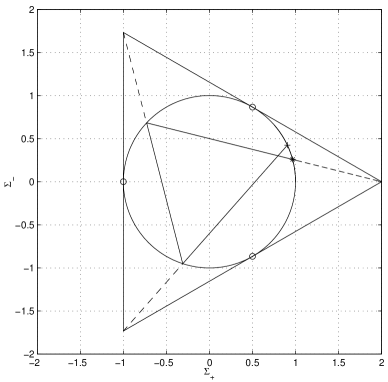
Figure 1. The Kasner map.

Let us begin with the non-stiff fluid case, including the vacuum case. We confine our attention to Bianchi IX solutions. The existence interval stretches back to $-\infty$ which corresponds to the singularity. There are some fixed points to which certain solutions converge, and data which lead to such solutions together with data of Taub type will be considered to be non-generic. The Kasner map, which is supposed to be an approximation of the Bianchi IX dynamics as one approaches a singularity, is illustrated in Figure 1. The circle in the $\Sigma_{+}\Sigma_{-}$-plane appearing in the figure is called the Kasner circle, and we have depicted two bounces of the Kasner map. The starting point is marked by a star, and the end point by a plus sign. Given a point $x$ on the Kasner circle, the Kasner map yields a new point $y$ on the Kasner circle by taking the corner of the triangle closest to $x$, drawing a straight line from the corner through $x$, and then letting $y$ be the second point of intersection between the line and the Kasner circle. One solid line corresponds to the closure of a vacuum type II orbit of the equations of Wainwright and Hsu. Actually, it is the projection of the closure of such an orbit to the $\Sigma_{+}\Sigma_{-}$-plane. A vacuum type II solution has one $N_{i}$ non-zero and the other zero, and the three different $N_{i}$ correspond to the three corners of the triangle; the rightmost corner corresponds to $N_{1}\neq 0$ and the corner on the top left corresponds to $N_{3}\neq 0$. The constraint (2.3) for the vacuum type II solutions is given by

$$\Sigma_{+}^{2}+\Sigma_{-}^{2}+\frac{3}{4}N_{i}^{2}=1.$$

The closure of this set is given a name in the following definition.

Definition 1.6.

The set

$$\mathcal{A}=\{(\Omega,\Sigma_{+},\Sigma_{-},N_{1},N_{2},N_{3}):\Omega+|N_{1}N_{2}|+|N_{2}N_{3}|+|N_{3}N_{1}|=0\}\cap M,$$

where $M$ is defined by (2.3), is called the Bianchi attractor.

The main result of this paper is that for generic Bianchi IX data, the solution converges to the attractor. That is

(1.9) $$\lim_{\tau\rightarrow-\infty}(\Omega+N_{1}N_{2}+N_{2}N_{3}+N_{3}N_{1})=0.$$

This conclusion supports the statement that the Kasner map approximates the dynamics, and also the statement that the matter content loses significance close to the singularity. Let us introduce some terminology.

Definition 1.7.

Let $f\in C^{\infty}(\mathbb{R}^{n},\mathbb{R}^{n})$, and consider a solution $x$ to the equation

$$\frac{dx}{dt}=f\circ x,\ x(0)=x_{0},$$

with maximal existence interval $(t_{-},t_{+})$. We call a point $x_{*}$ an $\alpha$-limit point of the solution $x$, if there is a sequence $t_{k}\rightarrow t_{-}$ with $x(t_{k})\rightarrow x_{*}$. The $\alpha$-limit set of $x$ is the set of its $\alpha$-limit points. The $\omega$-limit set is defined similarly by replacing $t_{-}$ with $t_{+}$.

Remark. If $t_{-}>-\infty$ then the $\alpha$-limit set is empty, cf. [16].

Thus, the $\alpha$-limit set of a generic solution is contained in the attractor. The desired statement is that the $\alpha$-limit set coincides with the attractor, but the best result we have achieved in this direction is that there must at least be three $\alpha$-limit points on the Kasner circle. This worst case situation corresponds to the solution converging to a periodic orbit of the Kasner map with period three. Observe that we have not proven anything concerning Bianchi VIII solutions.

Let us sketch the proof. It is natural to divide it into two parts. The first part consists of proving the existence of an $\alpha$-limit point on the Kasner circle. We achieve this in the following steps. First we analyze the $\alpha$-limit sets of the Bianchi types I, II and VI$\mathrm{I}_{0}$. An analysis of types I of II can also be found in Ellis and Wainwright [18]. Then we prove the existence of an $\alpha$-limit point for a generic Bianchi IX solution. To go from the existence of an $\alpha$-limit point to an $\alpha$-limit point on the Kasner circle, we use the analysis of the lower Bianchi types. In the second part, we prove (1.9). Let $d$ be the function appearing in that equation. We assume that $d$ does not converge to zero in order to reach a contradiction. The existence of an $\alpha$-limit point on the Kasner circle proves that there is a sequence $\tau_{k}\rightarrow-\infty$ such that $d(\tau_{k})\rightarrow 0$. If $d$ does not converge to zero there is a $\delta>0$, and a sequence $s_{k}\rightarrow-\infty$ such that $d(s_{k})\geq\delta$. We can assume $s_{k}\leq\tau_{k}$ and conclude that $d$ on the whole has to grow (going backwards) in the interval $[s_{k},\tau_{k}]$. What can be said about this growth? In Section 14, we prove that we can control the density parameter $\Omega$ in this process, assuming $\delta$ is small enough, which is not a restriction. As a consequence $\Omega$ can be assumed to be arbitrarily small during the growth. Some further arguments, given in Section 15, show that we can assume the growth to occur in the product $N_{2}N_{3}$, using the symmetries of the equations. Furthermore, one can assume the $\Sigma_{+}\Sigma_{-}$-variables to be arbitrarily close to $(\Sigma_{+},\Sigma_{-})=(-1,0)$, and that some expressions dominate others. For instance $1+\Sigma_{+}$ can be assumed to be arbitrarily much smaller than $N_{2}N_{3}$. This control introduces a natural concept of order of magnitude. The behaviour of the product $N_{2}N_{3}$ will be oscillatory; it will look roughly like a sine wave. The point is to prove that the product decays during a period of its oscillation; that would lead to a contradiction. The variation during a period can be expressed in terms of an integral, and we use the order of magnitude concept to prove an estimate showing that this integral has the right sign.

Now consider the stiff fluid case with positive density parameter. In this case we will consider Bianchi VIII and IX solutions. The analysis is similar for the other cases and a description of the results is to be found in Section 19. Again the singularity corresponds to $-\infty$. The density parameter $\Omega$ converges to a non-zero value, all the $N_{i}$ converge to zero, and in the $\Sigma_{+}\Sigma_{-}$-plane the solution converges to a point inside the triangle shown in Figure 2.

Figure 2. The triangle mentioned in the text.

In Section 2, we formulate the equations of Wainwright and Hsu and briefly describe their origin and some of their properties. Section 3 contains some elementary properties of solutions. We give the existence intervals of solutions to the equations, and prove that the $\Omega\Sigma_{+}\Sigma_{-}$-variables are contained in a compact set to the past for Bianchi IX solutions. As in the vacuum case, we also prove that $(\Sigma_{+},\Sigma_{-})$ can converge to $(-1,0)$ only if the solution is of Taub type, although this is no longer a characterization. In Section 4, we mention some critical points and make more precise the statement that solutions converging to these points are non-generic. Included in this section are also two technical lemmas relevant to the analysis. The monotonicity principle is explained in Section 5. It is fundamental to the analysis of the $\alpha$-limit sets of the solutions. We present two applications; the fact that all $\alpha$-limit points of Bianchi IX solutions are of type I, II or VI$\mathrm{I}_{0}$ and an analysis of the vacuum type II orbits. The last application is not complicated, but illustrates the arguments involved as well as demonstrating how the map depicted in Figure 1 can be viewed as a sequence of type II orbits. Section 6 deals with situations such that one has control over the shear variables and the density parameter. Specifically, it gives a geometric interpretation of some of the equations in $\Omega\Sigma_{+}\Sigma_{-}$-space. As an application, we prove that if a Bianchi IX solution has an $\alpha$-limit point on the Kasner circle then all the points obtained by applying the Kasner map to this point belong to the $\alpha$-limit set of the solution. The stiff fluid case is handled in Section 7. In this case the $\alpha$-limit set consists of a point regardless of type. Sections 8-10 deal with the lower order Bianchi types needed in order to analyze Bianchi IX. An analysis of types I of II can also be found in Ellis and Wainwright [18]. Section 11 gives the possibilities for a Taub type Bianchi IX solution. The technical Section 12 is needed in order to prove the existence of an $\alpha$-limit point for Bianchi IX solutions, and also to prove that the set of vacuum type II points is an attractor. It is used for approximating the solution in situations where the behaviour is oscillatory. Section 13 proves the existence of an $\alpha$-limit point for a Bianchi IX solution and the existence of an $\alpha$-limit point on the Kasner circle for generic Bianchi IX solutions. In Section 14, we prove that if one has control over the sum $|N_{1}N_{2}|+|N_{2}N_{3}|+|N_{3}N_{1}|$ in some time interval $[\tau_{1},\tau_{2}]$, and control over $\Omega$ in $\tau_{2}$ then one has control over $\Omega$ in the entire interval. This rather technical observation is essential in the proof that generic solutions converge to the attractor. The heart of this paper is Section 15 which contains a proof of (1.9). It also contains arguments that will be used in Section 16 to analyze the regularity of the set of non-generic points. In Section 17, we observe that the convergence to the attractor is uniform, and in Section 18 we prove the existence of at least three non-special $\alpha$-limit points on the Kasner circle. We formulate the main conclusions and prove Theorem 1.2 in Section 19. In Section 20, we relate our results concerning stiff fluid solutions to those of [2]. The appendices contain results relating solutions to the equations of Wainwright and Hsu with properties of the class A developments and some curvature computations.

2. Equations of Wainwright and Hsu

The essence of this paper is an analysis of the asymptotic behaviour of solutions to the equations of Wainwright and Hsu (2.1)-(2.3). One important property of these equations is that they describe all the Bianchi class A types at the same time. Another important property is that it seems that the variables remain in a compact set as one approaches a singularity. In the Bianchi IX case, this follows from the analysis presented in this paper. Let us give a rough description of the origin of the variables. In the situations we consider, there is a foliation of the Lorentz manifold by homogeneous spacelike hypersurfaces diffeomorphic to a Lie group $G$ of class A. One can define an orthonormal basis $e_{\alpha}$, $\alpha=0,...,3$, such that $e_{i}$, $i=1,2,3$, span the tangent space of the spacelike hypersurfaces of homogeneity, and $e_{0}=\partial_{t}$ for a suitable globally defined time coordinate $t$. It is possible to associate a matrix $n_{ij}$ with the spacelike vectors $e_{i}$, as in (1.7), and assume it to be diagonal with diagonal components $n_{i}$. One changes the time coordinate by $dt/d\tau=3/\theta$, where $\theta$ is minus the trace of the second fundamental form of the spacelike hypersurface corresponding to $t$. The $N_{i}(\tau)$ below are the $n_{i}(\tau)$ divided by $\theta(\tau)$, the $\Sigma_{+}$ and $\Sigma_{-}$ correspond to the traceless part of the second fundamental form of the spacelike hypersurface corresponding to $\tau$, similarly normalized, and finally $\Omega=3\mu/\theta^{2}$. We will refer to $\Sigma_{+}$ and $\Sigma_{-}$ as the shear variables, and to $\Omega$ as the density parameter. The question then arises to what extent this makes sense, since $\theta$ could become zero. An answer is given in the appendix. For all the Bianchi types except IX, this procedure is essentially harmless, and the variables of Wainwright and Hsu capture the entire Lorentz manifold. In the Bianchi IX case, there is however a point at which $\theta=0$, at least if $1\leq\gamma\leq 2$, see the appendix, and the variables are only valid for half a development in that case. As far as the analysis of the asymptotics are concerned, this is however not important. A derivation of the equations is given in the appendix. They are

$$N_{1}^{\prime} = (q-4\Sigma_{+})N_{1}$$

$$N_{2}^{\prime} = (q+2\Sigma_{+}+2\sqrt{3}\Sigma_{-})N_{2}$$

(2.1) $$N_{3}^{\prime} = (q+2\Sigma_{+}-2\sqrt{3}\Sigma_{-})N_{3}$$

$$\Sigma_{+}^{\prime} = -(2-q)\Sigma_{+}-3S_{+}$$

$$\Sigma_{-}^{\prime} = -(2-q)\Sigma_{-}-3S_{-}$$

$$\Omega^{\prime} = [2q-(3\gamma-2)]\Omega.$$

The prime denotes derivative with respect to a time coordinate $\tau$, and

$$q = \frac{1}{2}(3\gamma-2)\Omega+2(\Sigma_{+}^{2}+\Sigma_{-}^{2})$$

(2.2) $$S_{+} = \frac{1}{2}[(N_{2}-N_{3})^{2}-N_{1}(2N_{1}-N_{2}-N_{3})]$$

$$S_{-} = \frac{\sqrt{3}}{2}(N_{3}-N_{2})(N_{1}-N_{2}-N_{3}).$$

The constraint is

(2.3) $$\Omega+\Sigma_{+}^{2}+\Sigma_{-}^{2}+\frac{3}{4}[N_{1}^{2}+N_{2}^{2}+N_{3}^{2}-2(N_{1}N_{2}+N_{2}N_{3}+N_{3}N_{1})]=1.$$

We demand that $2/3<\gamma\leq 2$ and $\Omega\geq 0$. The equations (2.1)-(2.3) have certain symmetries, described in Wainwright and Hsu [17]. By permuting $N_{1},N_{2},N_{3}$ arbitrarily, we get new solutions, if we at the same time carry out appropriate combinations of rotations by integer multiples of $2\pi/3$, and reflections in the $(\Sigma_{+},\Sigma_{-})$-plane. Explicitly, the transformations

$$(\tilde{N}_{1},\tilde{N}_{2},\tilde{N}_{3})=(N_{3},N_{1},N_{2}),\ (\tilde{\Sigma}_{+},\tilde{\Sigma}_{-})=(-\frac{1}{2}\Sigma_{+}+\frac{1}{2}\sqrt{3}\Sigma_{-},-\frac{1}{2}\sqrt{3}\Sigma_{+}-\frac{1}{2}\Sigma_{-})$$

and

$$(\tilde{N}_{1},\tilde{N}_{2},\tilde{N}_{3})=(N_{1},N_{3},N_{2}),\ (\tilde{\Sigma}_{+},\tilde{\Sigma}_{-})=(\Sigma_{+},-\Sigma_{-})$$

yield new solutions. Below, we refer to rotations by integer multiples of $2\pi/3$ as rotations. Changing the sign of all the $N_{i}$ at the same time does not change the equations. Classify points $(\Omega,\Sigma_{+},\Sigma_{-},N_{1},N_{2},N_{3})$ according to the values of $N_{1},N_{2},N_{3}$ in the same way as in Table 1. Since the sets $N_{i}>0$, $N_{i}<0$ and $N_{i}=0$ are invariant under the flow of the equations, we may classify solutions to (2.1)-(2.3) accordingly.

Definition 2.1.

The Kasner circle is defined by the conditions $N_{i}=\Omega=0$ and the constraint (2.3). There are three points on this circle called special: $(\Sigma_{+},\Sigma_{-})=(-1,0)$ and $(1/2,\pm\sqrt{3}/2)$.

The following reformulation of $\Sigma_{+}^{\prime}$ is written down for future reference,

(2.4) $$\Sigma_{+}^{\prime}=-(2-2\Omega-2\Sigma_{+}^{2}-2\Sigma_{-}^{2})(\Sigma_{+}+1)-\frac{3}{2}(2-\gamma)\Omega\Sigma_{+}+\frac{9}{2}N_{1}(N_{1}-N_{2}-N_{3}).$$

3. Elementary properties of solutions

Here we collect some miscellaneous observations that will be of importance. Most of them are similar to results obtained in [16]. The $\alpha$-limit set defined in Definition 1.7 plays an important role in this paper, and here we mention some of its properties.

Lemma 3.1.

Let $f$ and $x$ be as in Definition 1.7. The $\alpha$-limit set of $x$ is closed and invariant under the flow of $f$. If there is a $T$ such that $x(t)$ is contained in a compact set for $t\leq T$, then the $\alpha$-limit set of $x$ is connected.

Proof. See e. g. [12]. $\Box$

Definition 3.1.

A solution to (2.1)-(2.3) satisfying $N_{2}=N_{3}$ and $\Sigma_{-}=0$, or one of the conditions found by applying the symmetries, is said to be of Taub type.

Remark. The set defined by $N_{2}=N_{3}$ and $\Sigma_{-}=0$ is invariant under the flow of (2.1).

Lemma 3.2.

The existence intervals for all solutions to (2.1)-(2.3) except Bianchi IX are $(-\infty,\infty)$. For Bianchi IX solutions we have past global existence.

Proof. As in the vacuum case, see [16]. $\Box$

By observations made in the appendix, $-\infty$ corresponds to the singularity.

Lemma 3.3.

Let $2/3<\gamma\leq 2$. Consider a solution of type IX. The image $(\Sigma_{+},\Sigma_{-},\Omega)((-\infty,0])$ is contained in a compact set whose size depends on the initial data. Further, if at a point in time $N_{3}\geq N_{2}\geq N_{1}$ and $N_{3}\geq 2$, then $N_{2}\geq N_{3}/10$.

Proof. As in the vacuum case, see [16]. $\Box$

That $(\Sigma_{+},\Sigma_{-},\Omega)$ is contained in a compact set for all the other types follows from the constraint. The second part of this lemma will be important in the proof of the existence of an $\alpha$-limit point. One consequence is that one $N_{i}$ may not become unbounded alone.

The final observation is relevant in proving curvature blow up. One can define a normalized version (22.3) of the Kretschmann scalar (1.8), and it can be expressed as a polynomial in the variables of Wainwright and Hsu. One way of proving that a specific solution exhibits curvature blow up is to prove that it has an $\alpha$-limit point at which the normalized Kretschmann scalar is non-zero. We refer to the appendix for the details. It turns out that this polynomial is zero when $N_{2}=N_{3}$, $N_{1}=0$, $\Sigma_{-}=0$, $\Sigma_{+}=-1$ and $\Omega=0$. The same is true of the points obtained by applying the symmetries. It is then natural to ask the question: for which solutions does $(\Sigma_{+},\Sigma_{-})$ converge to $(-1,0)$?

Proposition 3.1.

A solution to (2.1)-(2.3) with $2/3<\gamma<2$ satisfies

$$\lim_{\tau\rightarrow-\infty}(\Sigma_{+}(\tau),\Sigma_{-}(\tau))=(-1,0),$$

only if it is contained in the invariant set $\Sigma_{-}=0$ and $N_{2}=N_{3}$.

Remark. The proposition does not apply to the stiff fluid case. The analogous statements for the points $(\Sigma_{+},\Sigma_{-})=(1/2,\pm\sqrt{3}/2)$ are true by an application of the symmetries. We may not replace the implication with an equivalence, cf. Proposition 9.1.

Proof. The argument is essentially the same as in the vacuum case, see [16]. We only need to observe that $\Omega$ will decay exponentially when $(\Sigma_{+},\Sigma_{-})$ is close to $(-1,0)$. $\Box$

4. Critical points

Definition 4.1.

The critical point $F$ is defined by $\Omega=1$ and all other variables zero. In the case $2/3<\gamma<2$, we define the critical point $P_{1}^{+}(II)$ to be the type II point with $\Sigma_{-}=0$, $N_{1}>0$, $\Sigma_{+}=(3\gamma-2)/8$ and $\Omega=1-(3\gamma-2)/16$. The critical points $P_{i}^{+}(II)$, $i=2,3$ are found by applying the symmetries.

It will turn out that there are solutions which converge to these points as $\tau\rightarrow-\infty$. The main objective of this section is to prove that the set of such solutions is small. Observe that only non-vacuum solutions can converge these critical points.

Definition 4.2.

Let $\mathcal{I}_{\mathrm{VII}_{0}}$ denote initial data to (2.1)-(2.3) of type VI$\mathrm{I}_{0}$ with $\Omega>0$, and correspondingly for the other types. Let $\mathcal{P}_{\mathrm{VII}_{0}}$ be the elements of $\mathcal{I}_{\mathrm{VII}_{0}}$ such that the corresponding solutions converge to one of $P_{i}^{+}(II)$ as $\tau\rightarrow-\infty$ and similarly for Bianchi II and IX. Finally, let $\mathcal{F}_{\mathrm{VII}_{0}}$ be the elements of $\mathcal{I}_{\mathrm{VII}_{0}}$ such that the corresponding solutions converge to $F$ as $\tau\rightarrow-\infty$, and similarly for the other types.

Remark. The sets $\mathcal{F}_{\mathrm{II}}$ and so on depend on $\gamma$, but we omit this reference.

Observe that $\mathcal{I}_{\mathrm{I}}$, $\mathcal{I}_{\mathrm{II}}$, $\mathcal{I}_{\mathrm{VII}_{0}}$ and $\mathcal{I}_{\mathrm{IX}}$ are submanifolds of $\mathbb{R}^{6}$ of dimensions 2, 3, 4 and 5 respectively. They are diffeomorphic with open sets in a suitable $\mathbb{R}^{n}$; project $\Omega$ to zero. We will prove that $\mathcal{P}_{\mathrm{II}}$ consists of points and that $\mathcal{F}_{\mathrm{I}}$ is the point $F$. Let $2/3<\gamma<2$ be fixed. In Theorem 16.1, we will be able to prove that the sets $\mathcal{F}_{\mathrm{II}},\mathcal{F}_{\mathrm{VII}_{0}}$, $\mathcal{F}_{\mathrm{IX}}$, $\mathcal{P}_{\mathrm{VII}_{0}}$ and $\mathcal{P}_{\mathrm{IX}}$ are $C^{1}$ submanifolds of $\mathbb{R}^{6}$ of dimensions $1$, $2$, $3$, $1$ and $2$ respectively. This justifies the following definition.

Definition 4.3.

Let $2/3<\gamma<2$. A solution to (2.1)-(2.3) is said to be generic if it is not of Taub type, and if it does not belong to $\mathcal{F}_{\mathrm{I}},\mathcal{F}_{\mathrm{II}},\mathcal{F}_{\mathrm{VII}_{0}}$, $\mathcal{F}_{\mathrm{IX}}$, $\mathcal{P}_{\mathrm{II}}$, $\mathcal{P}_{\mathrm{VII}_{0}}$ or $\mathcal{P}_{\mathrm{IX}}$.

We will need the following two lemmas in the sequel.

Lemma 4.1.

Consider a solution $x$ to (2.1)-(2.3) such that $x$ has $P^{+}_{1}(II)$ as an $\alpha$-limit point but does not converge to it. Then $x$ has an $\alpha$-limit point of type II, which is not $P^{+}_{1}(II)$.

Remark. There is no solution satisfying the conditions of this lemma, but we will need it to establish that fact.

Proof. Consider the solution to belong to $\mathbb{R}^{6}$, and let the point $x_{0}$ represent $P^{+}_{1}(II)$. There is an $\epsilon>0$ such that for each $T$, there is a $\tau\leq T$ such that $x(\tau)$ does not belong to the open ball $B_{\epsilon}(x_{0})$. In $x_{0}$ one can compute that

$$q+2\Sigma_{+}\pm 2\sqrt{3}\Sigma_{-}>0.$$

Let $\epsilon$ be so small that these expressions are positive in $B_{\epsilon}(x_{0})$. Let $\tau_{k}\rightarrow-\infty$ be a sequence such that $x(\tau_{k})\rightarrow x_{0}$, and let $s_{k}\leq\tau_{k}$ be a sequence such that $x(s_{k})\in\partial B_{\epsilon}(x_{0})$ and $x((s_{k},\tau_{k}])\subseteq B_{\epsilon}(x_{0})$. Since $x(s_{k})$ is contained in a compact set, there is a convergent subsequence yielding an $\alpha$-limit point which is not $P^{+}_{1}(II)$. Since $N_{2}$ and $N_{3}$ converge to zero in $\tau_{k}$ and decay in absolute value from $\tau_{k}$ to $s_{k}$, the $\alpha$-limit point has to be of type II ($N_{1}$ has to be non-zero for the new $\alpha$-limit point if $\epsilon$ is small enough). $\Box$

Lemma 4.2.

Consider a solution $x$ to (2.1)-(2.3) such that $x$ has $F$ as an $\alpha$-limit point, but which does not converge to $F$. Then $x$ has an $\alpha$-limit point of type I which is not $F$.

Remark. The same remark as that made in connection with Lemma 4.1 holds concerning this lemma.

Proof. The idea is the same as the previous lemma. We need only observe that $q-4\Sigma_{+},\ q+2\Sigma_{+}+2\sqrt{3}\Sigma_{-}$ and $q+2\Sigma_{+}-2\sqrt{3}\Sigma_{-}$ are positive in $F$. $\Box$

5. The monotonicity principle

The following lemma will be a basic tool in the analysis of the asymptotics, we will refer to it as the monotonicity principle.

Lemma 5.1.

Consider

(5.1) $$\frac{dx}{dt}=f\circ x$$

where $f\in C^{\infty}(\mathbb{R}^{n},\mathbb{R}^{n})$. Let $U$ be an open subset of $\mathbb{R}^{n}$, and $M$ a closed subset invariant under the flow of the vectorfield $f$. Let $G:U\rightarrow\mathbb{R}$ be a continuous function such that $G(x(t))$ is strictly monotone for any solution $x(t)$ of (5.1), as long as $x(t)\in U\cap M$. Then no solution of (5.1) whose image is contained in $U\cap M$ has an $\alpha$- or $\omega$-limit point in $U$.

Remark. Observe that one can use $M=\mathbb{R}^{n}$. We will mainly choose $M$ to be the closed invariant subset of $\mathbb{R}^{6}$ defined by (2.3). If one $N_{i}$ is zero and two are non-zero, we consider the number of variables to be four etc.

Proof. Suppose $p\in U$ is an $\alpha$-limit point of a solution $x$ contained in $U\cap M$. Then $G\circ x$ is strictly monotone. There is a sequence $t_{n}\rightarrow t_{-}$ such that $x(t_{n})\rightarrow p$ by our supposition. Thus $G(x(t_{n}))\rightarrow G(p)$, but $G\circ x$ is monotone so that $G(x(t))\rightarrow G(p)$. Thus $G(q)=G(p)$ for all $\alpha$-limit points $q$ of $x$. Since $M$ is closed $p\in M$. The solution $\bar{x}$ of (5.1), with initial value $p$, is contained in $M$ by the invariance property of $M$, and it consists of $\alpha$-limit points of $x$ so that $G(\bar{x}(t))=G(p)$ which is constant. Furthermore, on an open set containing zero it takes values in $U$ contradicting the assumptions of the lemma. $\Box$

Let us give an example of an application.

Lemma 5.2.

Consider a solution to (2.1)-(2.3) of type VIII or IX. If it has an $\alpha$-limit point, then

$$\lim_{\tau\rightarrow-\infty}(N_{1}N_{2}N_{3})(\tau)=0.$$

Proof. Let $U$ of Lemma 5.1 be defined by the union of the sets $N_{i}\neq 0$, $i=1,2,3$, $M$ by the constraint (2.3), and $G$ by the function $N_{1}N_{2}N_{3}$. Compute

(5.2) $$(N_{1}N_{2}N_{3})^{\prime}=3qN_{1}N_{2}N_{3}.$$

Consider a solution $x$ of (2.1)-(2.3). We need to prove that $G\circ x$ is strictly monotone as long as $x(\tau)\in U\cap M$. By (5.2) the only problem that could occur is $q=0$. However, $q=0$ implies $|\Sigma_{+}^{\prime}|+|\Sigma_{-}^{\prime}|>0$ by (2.1)-(2.3) so that $G\circ x$ has the desired property. If the sequence $\tau_{k}\rightarrow-\infty$ yields the $\alpha$-limit point we assume exists, then we conclude that

$$(N_{1}N_{2}N_{3})(\tau_{k})\rightarrow 0.$$

Since $N_{1}N_{2}N_{3}$ is monotone, we conclude that it converges to zero. $\Box$

One important consequence of this observation is the fact that all $\alpha$-limit points of Bianchi VIII and IX solutions are of one of the lower Bianchi types. Since the $\alpha$-limit set is invariant under the flow, it is thus of interest to know something about the $\alpha$-limit sets of the lower Bianchi types, if one wants to prove the existence of an $\alpha$-limit point on the Kasner circle.

Let us now analyze the vacuum type II orbits and define the Kasner map.

Proposition 5.1.

A Bianchi II vacuum solution of (2.1)-(2.3) with $N_{1}>0$ and $N_{2}=N_{3}=0$ satisfies

(5.3) $$\lim_{\tau\rightarrow\pm\infty}N_{1}=0.$$

The $\omega$-limit set is a point in $\mathcal{K}_{1}$ and the $\alpha$-limit set is a point on the Kasner circle, in the complement of the closure of $\mathcal{K}_{1}$.

Remark. What is meant by $\mathcal{K}_{1}$ is explained in Definition 6.1.

Proof. Using the constraint (2.3) we deduce that

$$\Sigma_{+}^{\prime}=\frac{3}{2}N_{1}^{2}(2-\Sigma_{+}).$$

We wish to apply the monotonicity principle. There are three variables. Let $U$ be defined by $N_{1}>0$, $M$ be defined by (2.3), and $G(\Sigma_{+},\Sigma_{-},N_{1})=\Sigma_{+}$. We conclude that (5.3) is true as follows. Let $\tau_{n}\rightarrow\infty$. A subsequence yields an $\omega$-limit point by (2.3). The monotonicity principle yields $N_{1}(\tau_{n_{k}})\rightarrow 0$ for the subsequence. The argument for the $\alpha$-limit set is similar, and equation (5.3) follows. Combining this with the constraint, we deduce

$$\lim_{\tau\rightarrow\pm\infty}q=2.$$

Using the monotonicity of $\Sigma_{+}$, we conclude that $(\Sigma_{+},\Sigma_{-})$ has to converge. As for the $\alpha$-limit set, convergence to $\mathcal{K}_{1}$ is not allowed since $N_{1}^{\prime}<0$ close to $\mathcal{K}_{1}$. Convergence to one of the special points in the closure of $\mathcal{K}_{1}$ is also forbidden, since Proposition 3.1 would imply $N_{1}=0$ for the solution in that case. Assume now that $(\Sigma_{+},\Sigma_{-})\rightarrow(\sigma_{+},\sigma_{-})$ as $\tau\rightarrow\infty$. Compute

(5.4) $$\left(\frac{\Sigma_{-}}{2-\Sigma_{+}}\right)^{\prime}=0.$$

We get

(5.5) $$\frac{\Sigma_{-}}{2-\Sigma_{+}}=\frac{\sigma_{-}}{2-\sigma_{+}}$$

for arbitrary $(\Sigma_{+},\Sigma_{-})$ belonging to the solution. Since $N_{1}^{\prime}=(q-4\Sigma_{+})N_{1}$ and $N_{1}\rightarrow 0$, we have to have $\sigma_{+}\geq 1/2$. If $\sigma_{+}=1/2$, then $\sigma_{-}=\pm\sqrt{3}/2$. The two corresponding lines in the $\Sigma_{+}\Sigma_{-}$-plane, obtained by substituting $(\sigma_{+},\sigma_{-})$ into (5.5), do not intersect any points interior to the Kasner circle. Therefore $\sigma_{+}=1/2$ is not an allowed limit point, and the proposition follows. $\Box$

Observe that by (5.4), the projection of the solution to the $\Sigma_{+}\Sigma_{-}$-plane is a straight line. The orbits when $N_{2}>0$ and when $N_{3}>0$ are obtained by applying the symmetries. Figure 1 shows a sequence of vacuum type II orbits projected to the $\Sigma_{+}\Sigma_{-}$-plane. The first line, starting at the star, has $N_{1}>0$, the second $N_{3}>0$ and the third $N_{2}>0$.

Definition 5.1.

If $x_{0}$ is a non-special point on the Kasner circle, then the Kasner map applied to $x_{0}$ is defined to be the point $x_{1}$ on the Kasner circle, with the property that there is a vacuum type II orbit with $x_{0}$ as an $\omega$-limit point and $x_{1}$ as an $\alpha$-limit point.

6. Dependence on the shear variables

In several arguments, we will have control over the shear variables and the density parameter in some time interval, and it is of interest to know how the remaining variables behave in such situations. Consider for instance the expression multiplying $N_{1}$ in the formula for $N_{1}^{\prime}$, see (2.1). It is given by $q-4\Sigma_{+}$ and equals zero when

(6.1) $$\frac{1}{4}(3\gamma-2)\Omega+(1-\Sigma_{+})^{2}+\Sigma_{-}^{2}=1.$$

The set of points in $\Omega\Sigma_{+}\Sigma_{-}$-space satisfying this equation is a paraboloid, and the intersection with $\Omega=0$ is the dashed circle shown in Figure 3. If $(\Omega,\Sigma_{+},\Sigma_{-})$ belongs to the interior of the paraboloid (6.1) with $\Omega\geq 0$, then $|N_{1}|^{\prime}$ will be negative, so that $|N_{1}|$ increases as we go backward. Outside of the paraboloid, $|N_{1}|$ decreases. The situation is similar for $N_{2}$ and $N_{3}$. Observe that the circle obtained by letting $\Omega=0$ in (6.1) intersects the Kasner circle in two special points. The same is true of the rotated circles corresponding to $N_{2}$ and $N_{3}$. It will be convenient to introduce notation for the points on the Kasner circle at which $|N_{i}|^{\prime}$ is negative.

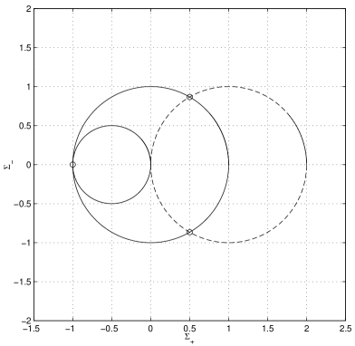
Figure 3. The circles mentioned in the text.

Definition 6.1.

We let $\mathcal{K}_{1},\ \mathcal{K}_{2}$ and $\mathcal{K}_{3}$ be the subsets of the Kasner circle where $q-4\Sigma_{+}<0,\ q+2\Sigma_{+}+2\sqrt{3}\Sigma_{-}<0$ and $q+2\Sigma_{+}-2\sqrt{3}\Sigma_{-}<0$ respectively.

Remark. On the Kasner circle, $\Omega=0$ so that $q=2(\Sigma_{+}^{2}+\Sigma_{-}^{2})=2$ under the conditions of this definition.

It also of interest to know when the derivatives of $N_{2}N_{3}$ and similar products are zero. Since $(N_{2}N_{3})^{\prime}=(2q+4\Sigma_{+})N_{2}N_{3}$, we consider the set on which $q+2\Sigma_{+}$ equals zero. This set is a paraboloid and is given by

$$\frac{1}{4}(3\gamma-2)\Omega+(\Sigma_{+}+\frac{1}{2})^{2}+\Sigma_{-}^{2}=\frac{1}{4}.$$

The intersection with the plane $\Omega=0$ is the circle with radius $1/2$ shown in Figure 3. Again, inside the paraboloid $|N_{2}N_{3}|$ increases as we go backward, and outside it decreases. There are corresponding paraboloids for the products $N_{1}N_{2}$ and $N_{1}N_{3}$. Observe that in the non-vacuum case, it is harmless to introduce $\omega=\Omega^{1/2}$ and then the paraboloids become half spheres.

Proposition 6.1.

Consider a Bianchi IX solution to (2.1)-(2.3) with $2/3<\gamma<2$. If the solution has a non-special $\alpha$-limit point $x$ on the Kasner circle, then the closure of the vacuum type II orbit with $x$ as an $\omega$-limit point belongs to the $\alpha$-limit set.

Remark. The same conclusion holds for a Bianchi type VI$\mathrm{I}_{0}$ solution with $N_{1}=0$, if it has an $\alpha$-limit point in $\mathcal{K}_{2}$ or $\mathcal{K}_{3}$.

Proof. Assume the limit point lies in $\mathcal{K}_{1}$ with $(\Sigma_{+},\Sigma_{-})=(\sigma_{+},\sigma_{-})$. There is a sequence $\tau_{k}\rightarrow-\infty$, such that the solution evaluated at $\tau_{k}$ converges to the point on the Kasner circle. There is a ball $B_{\eta}(\sigma_{+},\sigma_{-})$ in the $\Sigma_{+}\Sigma_{-}$-plane, centered at this point, such that $|N_{2}|,\ |N_{3}|,\ |N_{1}N_{2}|,\ |N_{1}N_{3}|$ and $\Omega$ all decay exponentially, at least as $e^{\xi\tau}$ for some fixed $\xi>0$, and $N_{1}$ increases exponentially, at least as $e^{-\xi\tau}$, in the closure of this ball. There is a $K$ such that $(\Sigma_{+}(\tau_{k}),\Sigma_{-}(\tau_{k}))\in B_{\eta}(\sigma_{+},\sigma_{-})$ for all $k\geq K$. For each time we enter the ball, we must leave it, since if we stay in it to the past, $N_{1}$ will grow to infinity whereas $N_{2}$ and $N_{3}$ will decay to zero, in violation of the constraint. Thus for each $\tau_{k}$, $k\geq K$, there is a $t_{k}\leq\tau_{k}$ corresponding to the first time we leave the ball, starting at $\tau_{k}$ and going backward. We may compute

$$(\frac{\Sigma_{-}}{2-\Sigma_{+}})^{\prime}=h$$

where

$$|h(\tau)|\leq\epsilon_{k}e^{\xi(\tau-\tau_{k})}$$

in $[t_{k},\tau_{k}]$ and $\epsilon_{k}\rightarrow 0$. Thus

$$\frac{\Sigma_{-}(\tau_{k})}{2-\Sigma_{+}(\tau_{k})}-\frac{\Sigma_{-}(t_{k})}{2-\Sigma_{+}(t_{k})}=\int_{t_{k}}^{\tau_{k}}hd\tau.$$

But

$$|\int_{t_{k}}^{\tau_{k}}hd\tau|\leq\frac{\epsilon_{k}}{\xi},$$

and in consequence

$$\frac{\Sigma_{-}(\tau_{k})}{2-\Sigma_{+}(\tau_{k})}-\frac{\Sigma_{-}(t_{k})}{2-\Sigma_{+}(t_{k})}\rightarrow 0.$$

We thus get a type II vacuum limit point with $N_{1}>0$, to which we may apply the flow, and deduce the conclusion of the lemma. The statement made in the remark follows in the same way. Observe that the only important thing was that the limit point was in $\mathcal{K}_{1}$ and $N_{1}$ was non-zero for the solution. $\Box$

7. The stiff fluid case

In this section we will assume $\Omega>0$ and $\gamma=2$ for all solutions we consider. We begin by explaining the origin of the triangle shown in Figure 2. Then we analyze the type II orbits. They yield an analogue of the Kasner map, connecting two points inside the Kasner circle, and we state an analogue of Proposition 6.1 for this map. We then prove that $\Omega$ is bounded away from zero to the past. Only in the case of Bianchi IX is an argument required, but this result is the central part of the analysis of the stiff fluid case. A peculiarity of the equations then yields the conclusion that $|N_{1}N_{2}|+|N_{2}N_{3}|+|N_{3}N_{1}|$ converges to zero exponentially. This proves that any solution is contained in a compact set to the past, and that all $\alpha$-limit points are of type I or II. Another consequence is that $\Omega$ has to converge to a non-zero value; this requires a proof in the Bianchi IX case. Next one concludes that all $N_{i}$ converge to zero, since if that were not the case, there would be an $\alpha$-limit point of type II to which one could apply the flow, obtaining $\alpha$-limit points with different $\Omega$:s. Then if a Bianchi IX solution had an $\alpha$-limit point outside the triangle, one could apply the ’Kasner’ map to such a point, obtaining an $\alpha$-limit point with some $N_{i}>0$. Finally, some technical arguments finish the analysis.

In the case of a stiff fluid, that is $\gamma=2$, it is convenient to introduce

$$\omega=\Omega^{1/2}.$$

We then have, since $3\gamma-2=4$,

(7.1) $$\omega^{\prime}=-(2-q)\omega.$$

The expression $\Omega+\Sigma_{+}^{2}+\Sigma_{-}^{2}$ turns into $\omega^{2}+\Sigma_{+}^{2}+\Sigma_{-}^{2}$, and the $\omega,\Sigma_{+},\Sigma_{-}$-coordinates of the type I points obey

(7.2) $$\omega^{2}+\Sigma_{+}^{2}+\Sigma_{-}^{2}=1,\ \omega\geq 0.$$

In the stiff fluid case, all the type I points are fixed points, and they play a role similar to that of the Kasner circle in the vacuum case.

Let us make some observations. If $N_{1}\neq 0$, then $N_{1}^{\prime}=0$ is equivalent to $q-4\Sigma_{+}=0$. Dividing by $2$ and completing squares, we see that this condition is equivalent to

(7.3) $$\omega^{2}+(1-\Sigma_{+})^{2}+\Sigma_{-}^{2}=1,\ \omega\geq 0.$$

By applying the symmetries, the conditions $N_{i}^{\prime}=0,\ N_{i}\neq 0$ are consequently all fulfilled precisely on half spheres of radii $1$. Since $|N_{1}|^{\prime}<0$ corresponds to an increase in $|N_{1}|$ as we go backward, $|N_{1}|$ increases exponentially as we are inside the half sphere (7.3) and decreases exponentially as we are outside it. If one takes the intersection of (7.2) and (7.3), one gets the subset $\Sigma_{+}=1/2$ of (7.2). The corresponding intersections for $N_{2}$ and $N_{3}$ yield two more lines in the $\Sigma_{+}\Sigma_{-}$-plane. Together they yield the triangle in Figure 2. Consequently, if $(\omega,\Sigma_{+},\Sigma_{-})$ is close to (7.2) and $(\Sigma_{+},\Sigma_{-})$ is in the interior of the triangle, then all the $N_{i}$ decay exponentially as $\tau\rightarrow-\infty$.

Let $\mathcal{M}_{1}$ be the subset $\omega\Sigma_{+}\Sigma_{-}$-space obeying (7.2) with $\omega>0$ and $\Sigma_{+}>1/2$ and $\mathcal{M}_{2}$, $\mathcal{M}_{3}$ be the corresponding sets for $N_{2}$ and $N_{3}$. We also let $\mathcal{L}_{1}$ be the subset of the intersection between (7.2) and (7.3) with $\omega>0$ and correspondingly $N_{2}$ and $N_{3}$ yield $\mathcal{L}_{2}$ and $\mathcal{L}_{3}$.

Lemma 7.1.

Consider a solution to (2.1)-(2.3) with $\gamma=2$ such that $N_{1}>0$, $\omega>0$ and $N_{2}=N_{3}=0$. Then

(7.4) $$\lim_{\tau\rightarrow\pm\infty}N_{1}(\tau)=0$$

and $(\omega,\Sigma_{+},\Sigma_{-})$ converges to a point, satisfying (7.2) and $\omega>0$, in the complement of $\mathcal{L}_{1}\cup\mathcal{M}_{1}$, as $\tau\rightarrow-\infty$. In $\omega\Sigma_{+}\Sigma_{-}$-space, the orbit of the solution is a straight line connecting two points satisfying (7.2). If $\omega>0$, it is strictly increasing along the solution, going backwards in time.

Proof. Since $q<2$ for the entire solution, we can apply the monotonicity principle with $U$ defined by $q<2$, $G$ defined by $\Sigma_{+}$ and $M$ by the constraint (2.3). If $q$ does not converge to 2 as $\tau\rightarrow-\infty$, we get an $\alpha$-limit point with $q<2$. We have a contradiction. This argument also yields the conclusion that $N_{1}\rightarrow 0$ as $\tau\rightarrow\infty$. Equation (7.4) follows. Observe that

(7.5) $$\Sigma_{+}^{\prime}=\frac{3}{2}N_{1}^{2}(2-\Sigma_{+}),\ \Sigma_{-}^{\prime}=-\frac{3}{2}N_{1}^{2}\Sigma_{-}$$

and

(7.6) $$\omega^{\prime}=-\frac{3}{2}N_{1}^{2}\omega.$$

Consequently, $\Sigma_{+}$, $\Sigma_{-}$ and $\omega$ are all monotone so that they converge, both as $\tau\rightarrow\infty$ and as $\tau\rightarrow-\infty$. It also follows from (7.5) and (7.6) that the quotients $(2-\Sigma_{+})/\omega$ and $\Sigma_{-}/\omega$ are constant. Thus the orbit in $\omega\Sigma_{+}\Sigma_{-}$-space describes a straight line connecting two points satisfying (7.2). As $\tau\rightarrow-\infty$, the solution cannot converge to a point in $\mathcal{L}_{1}\cup\mathcal{M}_{1}$ for the following reason. Assume it does. Since $\Sigma_{+}$ decreases as $\tau$ decreases, see (7.5), we must have $\Sigma_{+}\geq 1/2$ for the entire solution, since $\Sigma_{+}$ by assumption converges to a value $\geq 1/2$. But then $N_{1}^{\prime}<0$ for the entire solution by (2.1) and (2.3). Thus $N_{1}$ increases as we go backward, contradicting the fact that $N_{1}\rightarrow 0$. $\Box$

The next thing we wish to prove is that if a solution has an $\alpha$-limit point $x$ in the set $\mathcal{M}_{1}$, and $N_{1}\neq 0$ for the solution, then we can apply the ’Kasner’ map to that point. What we mean by that is that an entire type II orbit with $x$ as an $\omega$-limit point belongs to the $\alpha$-limit set of the original solution. From this one can draw quite strong conclusions. Observe for instance that by (7.1), $\omega$ is monotone for a Bianchi VIII solution to (2.1)-(2.3). Thus $\omega$ converges as $\tau\rightarrow-\infty$ since it is bounded. If the Bianchi VIII solution has an $\alpha$-limit point of type I outside the triangle, we can apply the Kasner map to it to obtain $\alpha$-limit points with different $\omega$. But that is impossible.

Lemma 7.2.

Consider a solution to (2.1)-(2.3) with $\gamma=2$ such that $N_{1}\neq 0$. Then if the solution has an $\alpha$-limit point $x\in\mathcal{M}_{1}$, the orbit of a type II solution with $x$ as an $\omega$-limit point belongs to the $\alpha$-limit set of the solution.

Proof. The proof is analogous to the proof of Proposition 6.1. $\Box$

Consider a solution such that $\omega>0$. We want to exclude the possibility that $\omega\rightarrow 0$ as $\tau\rightarrow-\infty$. Considering (7.1), we see that the only possibility for $\omega$ to decrease is if $q>2$. In that context, the following lemma is relevant.

Lemma 7.3.

Consider a Bianchi IX solution to (2.1)-(2.3) with $\gamma=2$. There is an $\alpha_{0}$ such that if $\alpha\leq\alpha_{0}$ and

$$(N_{1}N_{2}N_{3})(\tau)\leq\alpha,$$

then

$$q(\tau)-2\leq 4\alpha^{1/3}.$$

Proof. By a permutation of the variables, we can assume $N_{1}\leq N_{2}\leq N_{3}$ in $\tau$. Observe that

$$q-2\leq 3N_{1}(N_{2}+N_{3})$$

by the constraint (2.3). If $N_{3}\leq\alpha^{1/2}$ in $\tau$, we get $q-2\leq 6\alpha\leq 4\alpha^{1/3}$ if $\alpha_{0}$ is small enough. If $N_{3}\geq\alpha^{1/2}$ in $\tau$, we get

$$N_{1}N_{2}\leq\alpha^{1/2}.$$

Assume, in order to reach a contradiction, $(N_{1}N_{3})(\tau)\geq\alpha^{1/3}$. Then $N_{2}(\tau)\leq\alpha^{2/3}$, so that $N_{1}(\tau)\leq\alpha^{2/3}$ and $N_{3}(\tau)\geq\alpha^{-1/3}$. By Lemma 3.3 we get a contradiction if $\alpha_{0}$ is small enough. Thus

$$q-2\leq 3(N_{1}N_{2}+N_{1}N_{3})(\tau)\leq 3(\alpha^{1/3}+\alpha^{1/2})\leq 4\alpha^{1/3}$$

if $\alpha_{0}$ is small enough. $\Box$

For all solutions except those of Bianchi IX type, $\omega$ is monotone increasing as $\tau$ decreases. Thus, $\omega$ is greater than zero on the $\alpha$-limit set of any non-vacuum solution which is not of type IX. It turns out that the same is true for a Bianchi IX solution.

Lemma 7.4.

Consider a Bianchi IX solution to (2.1)-(2.3) with $\gamma=2$ such that $\omega>0$. Then there is an $\epsilon>0$ such that $\omega(\tau)\geq\epsilon$ for all $\tau\leq 0$.

Proof. Assume all the $N_{i}$ are positive. The function

$$\phi=\frac{(N_{1}N_{2}N_{3})^{1/3}}{\omega}$$

satisfies $\phi^{\prime}=2\phi$. Thus, for $\tau\leq 0$,

$$(N_{1}N_{2}N_{3})^{1/3}(\tau)=\omega(\tau)\phi(0)e^{2\tau}\leq Ce^{2\tau},$$

because of Lemma 3.3. For $\tau\leq T\leq 0$, we can thus apply Lemma 7.3, so that for $\tau\leq T$,

$$\int_{\tau}^{0}(q(s)-2)ds=\int_{\tau}^{T}(q(s)-2)ds+\int_{T}^{0}(q(s)-2)ds\leq 4C\int_{\tau}^{T}e^{2s}ds+$$

$$+\int_{T}^{0}(q(s)-2)ds\leq 2Ce^{2T}+\int_{T}^{0}(q(s)-2)ds\leq C^{\prime}<\infty.$$

Consequently,

$$\omega(\tau)=\omega(0)\exp(-\int_{\tau}^{0}(q(s)-2)ds)\geq\omega(0)e^{-C^{\prime}},$$

and the lemma follows. $\Box$

The next lemma will be used to prove that $\omega$ converges for a Bianchi IX solution.

Lemma 7.5.

Consider a solution to (2.1)-(2.3) with $\gamma=2$ and $\omega>0$. Then there is an $\alpha>0$ and a $T$ such that

$$|N_{1}N_{2}|+|N_{2}N_{3}|+|N_{3}N_{1}|\leq e^{\alpha\tau}$$

for all $\tau\leq T$.

Proof. Consider $g=|N_{2}N_{3}|/\omega$. Then

$$g^{\prime}=(2\omega^{2}+2(1+\Sigma_{+})^{2}+2\Sigma_{-}^{2})g.$$

Since $\omega(\tau)\geq\epsilon$ for all $\tau\leq 0$, we conclude that

$$g(\tau)\leq g(0)\exp(2\epsilon^{2}\tau)$$

so that

$$|(N_{2}N_{3})(\tau)|\leq g(0)\omega(\tau)\exp(2\epsilon^{2}\tau).$$

There are similar estimates for the other products. By Lemma 3.3, we know that $\omega$ is bounded in $(-\infty,0]$ so that by choosing $\alpha=\epsilon^{2}$ and $T$ negative enough the lemma follows. $\Box$

Corollary 7.1.

Consider a solution to (2.1)-(2.3) with $\gamma=2$ and $\omega>0$. Then $(\omega,\Sigma_{+},\Sigma_{-},N_{1},N_{2},N_{3})(-\infty,0]$ is contained in a compact set and all the $\alpha$-limit points are of type I or II.

Lemma 7.6.

Consider a solution to (2.1)-(2.3) with $\gamma=2$ and $\omega>0$. Then

$$\lim_{\tau\rightarrow-\infty}\omega(\tau)=\omega_{0}>0.$$

Proof. Since this follows from the monotonicity of $\omega$ in all cases except Bianchi IX, see (7.1), we assume that the solution is of type IX. Let $\tau_{k}\rightarrow-\infty$ be a sequence such that $\omega(\tau_{k})\rightarrow\omega_{1}>0$. This is possible since $\omega$ is constrained to belong to a compact set for $\tau\leq 0$ by Lemma 3.3, and since $\omega$ is bounded away from zero to the past by Lemma 7.4. Assume $\omega$ does not converge to $\omega_{1}$. Then there is a sequence $s_{k}\rightarrow-\infty$ such that $\omega(s_{k})\rightarrow\omega_{2}$ where we can assume $\omega_{2}>\omega_{1}$. We can also assume $\tau_{k}\leq s_{k}$. Then

$$\omega(s_{k})=\exp(\int_{\tau_{k}}^{s_{k}}(q-2)ds)\omega(\tau_{k}).$$

Since

$$q-2\leq 3(N_{1}N_{2}+N_{2}N_{3}+N_{3}N_{1})\leq 3e^{\alpha\tau}$$

for $\tau\leq T$ by Lemma 7.5 and the constraint (2.3), we have, assuming $s_{k}\leq T$,

$$\int_{\tau_{k}}^{s_{k}}(q-2)ds\leq 3\int_{\tau_{k}}^{s_{k}}e^{\alpha\tau}d\tau\leq\frac{3}{\alpha}e^{\alpha s_{k}}.$$

Thus

$$\omega(s_{k})\leq\exp(\frac{3}{\alpha}e^{\alpha s_{k}})\omega(\tau_{k})\rightarrow\omega_{1},$$

so that $\omega_{2}\leq\omega_{1}$ contradicting our assumption. $\Box$

Corollary 7.2.

Consider a solution to (2.1)-(2.3) with $\gamma=2$ and $\omega>0$. Then

$$\lim_{\tau\rightarrow-\infty}N_{i}(\tau)=0$$

for $i=1,2,3$.

Proof. Assume $N_{1}$ does not converge to zero. Then there is a type II $\alpha$-limit point with $N_{1}$ and $\omega$ non-zero by Corollary 7.1 and Lemma 7.6. If we apply the flow, we get $\alpha$-limit points with different $\omega$ in contradiction to Lemma 7.6. $\Box$

Lemma 7.7.

Consider a solution to (2.1)-(2.3) with $\gamma=2$ and $\omega>0$. If it has an $\alpha$-limit point of type I inside the triangle, the solution converges to that point.

Proof. Let $x$ be the limit point. Let $B$ be a ball of radius $\epsilon$ in $\omega\Sigma_{+}\Sigma_{-}$-space, with center given by the $\omega,\Sigma_{+},\Sigma_{-}$-coordinates of $x$. Let $\tau_{k}\rightarrow-\infty$ be a sequence that yields $x$. Assume the solution leaves $B$ to the past of every $\tau_{k}$. Then there is a sequence $s_{k}\rightarrow-\infty$, such that the $\omega,\Sigma_{+},\Sigma_{-}$-coordinates of the solution evaluated in $s_{k}$ converges to a point on the boundary of $B$, $s_{k}\leq\tau_{k}$, and the $\omega,\Sigma_{+},\Sigma_{-}$-coordinates of the solution are contained in $B$ during $[s_{k},\tau_{k}]$, $k$ large enough.

Since all expressions in the $N_{i}$ decay exponentially as $e^{\alpha\tau}$, for some $\alpha>0$, as long as the $\omega,\Sigma_{+},\Sigma_{-}$-coordinates are in $B$ ($\epsilon$ small enough), we have

$$|\Sigma_{+}^{\prime}|+|\Sigma_{-}^{\prime}|+|\omega^{\prime}|\leq\alpha_{k}e^{\alpha(\tau-\tau_{k})}$$

for $\tau\in[s_{k},\tau_{k}]$ where $\alpha_{k}\rightarrow 0$. We get

$$|\Sigma_{+}(\tau_{k})-\Sigma_{+}(s_{k})|\leq\frac{\alpha_{k}}{\alpha}\rightarrow 0,$$

and similarly for $\Sigma_{-}$ and $\omega$. The assumption that we always leave $B$ consequently yields a contradiction. We must thus converge to the given $\alpha$-limit point. $\Box$

Proposition 7.1.

Consider a solution to (2.1)-(2.3) with $\gamma=2$ and $\omega>0$. If $N_{i}$ is non-zero for the solution, it converges to a type I point in the complement of $\mathcal{M}_{i}$ with $\omega>0$.

Proof. If there is an $\alpha$-limit point on $\mathcal{M}_{i}$, we can use Lemma 7.2 to obtain a contradiction to Lemma 7.6. If there is an $\alpha$-limit point in $\mathcal{M}_{k}$ and $N_{k}$ is zero for the solution, the solution converges to that point by an argument similar to the one given in the previous lemma. What remains is the possibility that all the $\alpha$-limit points are on the $\mathcal{L}_{k}$. Since $\omega$ converges, the possible points projected to the $\Sigma_{+}\Sigma_{-}$-plane are the intersection between a triangle and a circle. Since the $\alpha$-limit set is connected, we conclude that the solution must converge to a point on one of the $\mathcal{L}_{k}$. $\Box$

Proposition 7.2.

Consider a solution to (2.1)-(2.3) with $\gamma=2$ and $\omega>0$. If $N_{i}$ is non-zero for the solution, the solution cannot converge to a point in $\mathcal{L}_{i}$.

Proof. Assume $i=1$. Then $\mathcal{L}_{i}$ is the subset of (7.2) consisting of points with $\Sigma_{+}=1/2$ and $\omega>0$. Since $N_{2},\ N_{3},\ N_{2}N_{3},\ N_{2}N_{1}$ and $N_{3}N_{1}$ converge to zero faster than $N_{1}^{2}$, $\Sigma_{+}^{\prime}$ will in the end be positive, cf. (7.5), so that there is a $T$ such that $\Sigma_{+}(\tau)\geq 1/2$ for $\tau\leq T$. Since $N_{1}$ will dominate in the end, we can also assume $q(\tau)<2$ for $\tau\leq T$. By (2.1) we conclude that $|N_{1}|$ increases backward as $\tau\leq T$ contradicting Corollary 7.2. $\Box$

Adding up the last two propositions, we conclude that the $\Sigma_{+}\Sigma_{-}$-variables of Bianchi VIII and IX solutions converge to a point interior to the triangle of Figure 2, and $\Omega$ to the value then determined by the constraint (2.3). In the Bianchi VI$\mathrm{I}_{0}$ case, a side of the triangle disappears, increasing the set of points to which $\Sigma_{+},\Sigma_{-}$ may converge. We sum up the conclusions in Section 19.

8. Type I solutions

Consider type I solutions ($N_{i}=0$). The point $F$ and the points on the Kasner circle are fixed points. Consider a solution with $0<\Omega(\tau_{0})<1$. Using the constraint, we may express the time derivative of $\Omega$ in terms of $\Omega$. Solving the resulting equation yields

$$\lim_{\tau\rightarrow-\infty}\Omega(\tau)=0,\ \lim_{\tau\rightarrow\infty}\Omega(\tau)=1.$$

By (2.1) $(\Sigma_{+},\Sigma_{-})$ moves radially.

Proposition 8.1.

For a type I solution, with $2/3<\gamma<2$, which is not F, we have

$$\lim_{\tau\rightarrow-\infty}(\Sigma_{+},\Sigma_{-},\Omega)(\tau)=(\sigma_{+}/|\sigma|,\sigma_{-}/|\sigma|,0),$$

where $(\sigma_{+},\sigma_{-})$ is the initial value of $(\Sigma_{+},\Sigma_{-})$, and $|\sigma|$ is the Euclidean norm of the initial value.

9. Type II solutions

Proposition 9.1.

Consider a type II solution with $N_{1}>0$ and $2/3<\gamma<2$. If the initial value for $\Sigma_{-}$ is non-zero, the $\alpha$-limit set is a point in $\mathcal{K}_{2}\cup\mathcal{K}_{3}$. If the initial value for $\Sigma_{-}$ is zero, either the solution is the special point $P_{1}^{+}(II)$, it is contained in $\mathcal{F}_{\mathrm{II}}$, or

(9.1) $$\lim_{\tau\rightarrow-\infty}(\Omega,\Sigma_{+},N_{1})(\tau)=(0,-1,0).$$

Proof. Let the initial data be given by $(\sigma_{+},\sigma_{-},\Omega_{0})$. The vacuum case was handled in Proposition 5.1, so we will assume $\Omega_{0}>0$.

Consider first the case $\sigma_{-}\neq 0$. Compute

$$q-2=-\frac{3}{2}(2-\gamma)\Omega-\frac{3}{2}N_{1}^{2}.$$

Thus, $\Sigma_{-}$ decreases if it is negative, and increases if it is positive, as we go backward in time, by (2.1). Thus, both $N_{1}$ and $\Omega$ must converge to $0$ as $\tau\rightarrow-\infty$, since the variables are constrained to belong to a compact set, and because of the monotonicity principle. Since $\Sigma_{-}$ is monotonous and the $\alpha$-limit set is connected, see Lemma 3.1, $(\Sigma_{+},\Sigma_{-})$ must converge to a point, say $(s_{+},s_{-})$ on the Kasner circle. We must have $s_{-}\neq 0$, and

$$2s_{+}^{2}+2s_{-}^{2}-4s_{+}\geq 0,$$

since $N_{1}$ converges to $0$. There are two special points in this set, but we may not converge to them, since that would imply $N_{1}=0$ for the entire solution by Proposition 3.1. The first part of the proposition follows.

Consider the case $\sigma_{-}=0$. There is a fixed point $P_{1}^{+}(II)$. Eliminating $\Omega$ from (2.1)-(2.3), we are left with the two variables $N_{1}$ and $\Sigma_{+}$. The linearization has negative eigenvalues at $P_{1}^{+}(II)$, so that no solution which does not equal $P_{1}^{+}(II)$ can have it as an $\alpha$-limit point, cf. [10] pp. 228-234. There is also a set of solutions converging to the fixed point $F$. Consider now the complement of the above. The function

$$Z_{7}=\frac{N_{1}^{2m}\Omega^{1-m}}{(1-v\Sigma_{+})^{2}},$$

where $v=(3\gamma-2)/8$ and $m=3v(2-\gamma)/8(1-v^{2})$, found by Uggla satisfies

$$Z_{7}^{\prime}=\frac{3(2-\gamma)}{1-v\Sigma_{+}}\frac{1}{1-v^{2}}(\Sigma_{+}-v)^{2}Z_{7}.$$

Apply the monotonicity principle. Let $G=Z_{7}$ and $U$ be defined as the subset of $\Omega\Sigma_{+}N_{1}$-space consisting of points different from $P_{1}^{+}(II)$, which have $\Omega>0$, $N_{1}>0$ and $|\Sigma_{+}|<1$. Let $M$ be defined by the constraint. If $\Sigma_{+}=v$ then $Z_{7}^{\prime}=0$, but if we are not at $P_{1}^{+}(II)$, $\Sigma_{+}=v$ implies $\Sigma_{+}^{\prime}\neq 0$. Thus, $G\circ x$ is strictly monotone as long as $x$ is contained in $U\cap M$. Since the solution cannot have $P_{1}^{+}(II)$ as an $\alpha$-limit point, we must thus have $N_{1}=0$ or $\Omega=0$ in the $\alpha$-limit set. Observe that

(9.2) $$\Sigma_{+}^{\prime}=\frac{3}{2}N_{1}^{2}(2-\Sigma_{+})-\frac{3}{2}(2-\gamma)\Omega\Sigma_{+}.$$

Thus, if the solution attains a point $\Sigma_{+}\leq 0$, then (9.1) holds. We will now prove that this is the only possibility.

a. Assume we have an $\alpha$-limit point with $N_{1}>0$ and $\Omega=0$. Then we may apply the flow to that limit point to get $\Sigma_{+}=-1$ as a limit point, but then the solution must attain $\Sigma_{+}\leq 0$.

b. If $\Omega>0$ but $N_{1}=0$, then we may assume $\Sigma_{+}\neq 0$ since we are not on $\mathcal{F}_{\mathrm{II}}$, cf. Lemma 4.2. Apply the flow to arrive at $\Sigma_{+}=-1$ or $\Sigma_{+}=1$. The former alternative has been dealt with, and the latter case allows us to construct an $\alpha$-limit point with $N_{1}>0$ and $\Omega=0$, since $N_{1}$ increases exponentially, and $\Omega$ decreases exponentially, in a neighbourhood of the point on the Kasner circle with $\Sigma_{+}=1$, cf. Proposition 6.1.

c. The situation $\Omega=N_{1}=0$ can be handled as above. $\Box$

We make one more observation that will be relevant in analyzing the regularity of $\mathcal{F}_{\mathrm{II}}$.

Lemma 9.1.

The closure of $\mathcal{F}_{\mathrm{II}}$ does not intersect $\mathcal{A}$.

Proof. Assume there is a sequence $x_{k}\in\mathcal{F}_{\mathrm{II}}$ such that the distance from $x_{k}$ to $\mathcal{A}$ goes to zero. We can assume that all the $x_{k}$ have $N_{1}>0$ by choosing a suitable subsequence and then applying the symmetries. We can also assume that $x_{k}\rightarrow x\in\mathcal{A}$. Since $\Sigma_{-}=0$ for all the $x_{k}$ by Proposition 9.1, the same holds for $x$. Observe that no element of $\mathcal{F}_{\mathrm{II}}$ can have $\Sigma_{+}\leq 0$, because of (9.2). If $N_{1}$ corresponding to $x$ is zero, we then conclude that $x$ is defined by $\Sigma_{+}=1$ and all the other variables zero. Applying the flow to the past to the points $x_{k}$ will then yield a sequence $y_{k}\in\mathcal{F}_{\mathrm{II}}$ such that $y_{k}$ converges to a type II vacuum point with $N_{1}>0$ and $\Sigma_{-}=0$, cf. the proof of Proposition 6.1. Thus, we can assume that the limit point $x\in\mathcal{A}$ has $N_{1}>0$. Applying the flow to $x$ yields the point $\Sigma_{+}=-1$ on the Kasner circle by Proposition 5.1. By the continuity of the flow, we can apply the flow to $x_{k}$ to obtain elements in $\mathcal{F}_{\mathrm{II}}$ with $\Sigma_{+}<0$ which is impossible. $\Box$

10. Type VI$\mathrm{I}_{0}$ solutions

When speaking of Bianchi VI$\mathrm{I}_{0}$ solutions, we will always assume $N_{1}=0$ and $N_{2},N_{3}>0$. Consider first the case $N_{2}=N_{3}$ and $\Sigma_{-}=0$

Proposition 10.1.

Consider a type VI$I_{0}$ solution with $N_{1}=0$ and $2/3<\gamma<2$. If $N_{2}=N_{3}$ and $\Sigma_{-}=0$, one of the following possibilities occurs

1. The solution converges to $\Sigma_{+}=1$ on the Kasner circle.

2. The solution converges to $F$.

3. $\lim_{\tau\rightarrow-\infty}\Sigma_{+}=-1,\ \lim_{\tau\rightarrow-\infty}N_{2}=n_{2}>0,\ \lim_{\tau\rightarrow-\infty}\Omega=0$.

Proof. Since

$$\Sigma_{+}^{\prime}=-\frac{3}{2}(2-\gamma)\Omega\Sigma_{+}$$

if $N_{2}=N_{3}$, the conclusions of the lemma follow, except for the statement that $N_{2}$ converges to a non-zero value if $\Sigma_{+}$ converges to $-1$. However, $\Omega$ will decay to zero exponentially close to the Kasner circle, and by the constraint, $1+\Sigma_{+}$ will behave as $\Omega$ close to $\Sigma_{+}=-1$. Thus, $q+2\Sigma_{+}$ will be integrable. $\Box$

Before we state a proposition concerning the behaviour of generic Bianchi VI$\mathrm{I}_{0}$ solutions, let us give an intuitive picture. Figure 4 shows a simulation with $\gamma=1$, where the plus sign represents the starting point, and the star the end point, going backward. $\Omega$ will decay to zero quite rapidly, and the same holds for the product $N_{2}N_{3}$. In that sense, the solution will asymptotically behave like a sequence of type II vacuum orbits. If both $N_{2}$ and $N_{3}$ are small, and we are close to the section $\mathcal{K}_{2}$ on the Kasner circle, then $N_{2}$ will increase exponentially, and $N_{3}$ will decay exponentially, yielding in the end roughly a type II orbit with $N_{2}>0$. If this orbit ends in at a point in $\mathcal{K}_{3}$, then the game begins anew, and we get roughly a type II orbit with $N_{3}>0$. Observe however that if we get close to $\mathcal{K}_{1}$, there is nothing to make us bounce away, since $N_{1}$ is zero. The simulation illustrates this behaviour. Consider the figure of the solution projected to the $\Sigma_{+}\Sigma_{-}$-plane. The three points that appear to be on the Kasner circle are close to $\mathcal{K}_{2}$, $\mathcal{K}_{3}$ and $\mathcal{K}_{1}$ respectively. Observe how this correlates with the graphs of $N_{2}$, $N_{3}$ and $q$.

Figure 4. Illustration of a Bianchi VI$\mathrm{I}_{0}$ solution.

Proposition 10.2.

Generic Bianchi VI$I_{0}$ solutions with $N_{1}=0$ and $2/3<\gamma<2$ converge to a point in $\mathcal{K}_{1}$.

We divide the proof into lemmas. First we prove that the past dynamics are contained in a compact set.

Lemma 10.1.

For a generic Bianchi VI$I_{0}$ solution with $N_{1}=0$ and $2/3<\gamma<2$, $(N_{2},N_{3})(-\infty,0]$ is contained in a compact set.

Proof. For a generic solution,

$$Z_{-1}=\frac{\frac{4}{3}\Sigma_{-}^{2}+(N_{2}-N_{3})^{2}}{N_{2}N_{3}}$$

is never zero. Compute

(10.1) $$Z_{-1}^{\prime}=-\frac{16}{3}\frac{\Sigma_{-}^{2}(1+\Sigma_{+})}{\frac{4}{3}\Sigma_{-}^{2}+(N_{2}-N_{3})^{2}}Z_{-1}.$$

The proof that the past dynamics are contained in a compact set is as in Rendall [15]. Let $\tau\leq 0$. Then

$$Z_{-1}(\tau)\geq Z_{-1}(0),$$

so that

$$(N_{2}N_{3})(\tau)\leq\frac{4}{3Z_{-1}(0)}.$$

Combining this fact with the constraint, we see that all the variables are contained in a compact set during $(-\infty,0]$. $\Box$

We now prove that $N_{2}N_{3}\rightarrow 0$. The reason being the desire to reduce the problem by proving that all the limit points are of type I or II, and then use our knowledge about what happens when we apply the flow to such points.

Lemma 10.2.

Generic Bianchi VI$I_{0}$ solutions with $N_{1}=0$ and $2/3<\gamma<2$ satisfy

$$\lim_{\tau\rightarrow-\infty}(N_{2}N_{3})(\tau)=0.$$

Proof. Assume the contrary. Then we can use Lemma 10.1 to construct an $\alpha$-limit point $(\omega,\sigma_{+},\sigma_{-},0,n_{2},n_{3})$ where $n_{2}n_{3}>0$. We apply the monotonicity principle in order to arrive at a contradiction. With notation as in Lemma 5.1, let $U$ be defined by $N_{2}>0,\ N_{3}>0$ and $\Sigma_{-}^{2}+(N_{2}-N_{3})^{2}>0$. Let $G$ be defined by $Z_{-1}$, and $M$ by the constraint (2.3). We have to show that $G$ evaluated on a solution is strictly monotone as long as the solution is contained in $U\cap M$. Consider (10.1). By the constraint (2.3), $\Sigma_{-}^{2}+(N_{2}-N_{3})^{2}>0$ implies $\Sigma_{+}>-1$. Furthermore, $Z_{-1}>0$ on $U$. If $Z_{-1}^{\prime}=0$ in $U\cap M$, we thus have $\Sigma_{-}=0$, but then $\Sigma_{-}^{\prime}\neq 0$ since $\Sigma_{-}^{2}+(N_{2}-N_{3})^{2}>0$ and $N_{2}+N_{3}>0$. The $\alpha$-limit point we have constructed cannot belong to $U$. On the other hand, $n_{2},n_{3}>0$ and since $Z_{-1}$ increases as we go backward, $\sigma_{-}^{2}+(n_{2}-n_{3})^{2}$ cannot be zero. We have a contradiction. $\Box$

Proof of Proposition 10.2. Compute

(10.2) $$\Sigma_{+}^{\prime}=-(2-2\Omega-2\Sigma_{+}^{2}-2\Sigma_{-}^{2})(1+\Sigma_{+})-\frac{3}{2}(2-\gamma)\Omega\Sigma_{+}$$

by (2.4). Assume we are not on $\mathcal{P}_{\mathrm{VII}_{0}}$ or $\mathcal{F}_{\mathrm{VII}_{0}}$. Let us first prove that there is an $\alpha$-limit point on the Kasner circle. Assume $F$ is an $\alpha$-limit point. Then we may construct a type I limit point which is not $F$, and thus a limit point on the Kasner circle, cf. Lemma 4.2 and Proposition 8.1. By Lemma 10.2, we may then assume that there is a limit point of type I or II, which is not $P_{2}^{+}(II)$ or $P_{3}^{+}(II)$, and does not lie in $\mathcal{F}_{\mathrm{I}}$ or $\mathcal{F}_{\mathrm{II}}$, cf. Lemma 4.1. Thus, we get a limit point on the Kasner circle by Proposition 8.1 and Proposition 9.1.

Next, we prove that there has to be an $\alpha$-limit point which lies in the closure of $\mathcal{K}_{1}$. If the $\alpha$-limit point we have constructed is in $\mathcal{K}_{2}$ or $\mathcal{K}_{3}$, we can apply the Kasner map according to the remark following Proposition 6.1. After a finite number of Kasner iterates we will end up in the desired set. If the $\alpha$-limit point we obtained has $\Sigma_{+}=-1$, we may construct a limit point with $1+\Sigma_{+}=\epsilon>0$ by Proposition 3.1. We can also assume that $\Omega=0$ for this point, since $\Omega$ decays exponentially going backward when $\Sigma_{+}$ is close to $-1$. By Lemma 10.2, this limit point will be a type I or II vacuum point, and by applying the flow we get a non special limit point on the Kasner circle. As above, we then get an $\alpha$-limit point in the desired set. Let the $\Sigma_{+}\Sigma_{-}$-variables of one $\alpha$-limit point in the closure of $\mathcal{K}_{1}$ be $(\sigma_{+},\sigma_{-})$.

By (10.2), we conclude that once $\Sigma_{+}$ has become greater than $0$, it becomes monotone so that it has to converge. Moreover, we see by the same equation that $\Omega$ then has to converge to zero, and $\Sigma_{+}^{2}+\Sigma_{-}^{2}$ has to converge to $1$. Since the $\alpha$-limit set is connected, by Lemma 3.1 and Lemma 10.1, we conclude that $(\Sigma_{+},\Sigma_{-})$ has to converge to $(\sigma_{+},\sigma_{-})$. By Proposition 3.1, $(\sigma_{+},\sigma_{-})$ cannot equal $(1/2,\pm\sqrt{3}/2)$, since otherwise $N_{2}$ or $N_{3}$ would be zero for the entire solution. Consequently, $\sigma_{+}>1/2$, and we conclude that $N_{2}$ and $N_{3}$ have to converge to zero. The proposition follows. $\Box$

11. Taub type IX solutions

Consider the Taub type solutions: $\Sigma_{-}=0$ and $N_{2}=N_{3}$. We prove that except for the cases when the solution belongs to $\mathcal{F}_{\mathrm{IX}}$ or $\mathcal{P}_{\mathrm{IX}}$, $(\Sigma_{+},\Sigma_{-})$ converges to $(-1,0)$.

Lemma 11.1.

Consider a type IX solution with $\Sigma_{-}=0$, $N_{2}=N_{3}$ and $2/3<\gamma<2$. Then $\Sigma_{+}(\tau_{0})\leq 0$ and $\Omega(\tau_{0})<1$ imply

$$\lim_{\tau\rightarrow-\infty}(\Omega,\Sigma_{+},\Sigma_{-},N_{1},N_{2},N_{3})(\tau)=(0,-1,0,0,n_{2},n_{2}),$$

where $0<n_{2}<\infty$.

Proof. We prove that the flow will take us to the boundary of the parabola $\Omega+\Sigma_{+}^{2}=1$ with $\Sigma_{+}<0$, and that we will then slide down the side on the outside to reach $\Sigma_{+}=-1$, see Figure 5. The plus sign in the figure represents the starting point, and the star the end point.

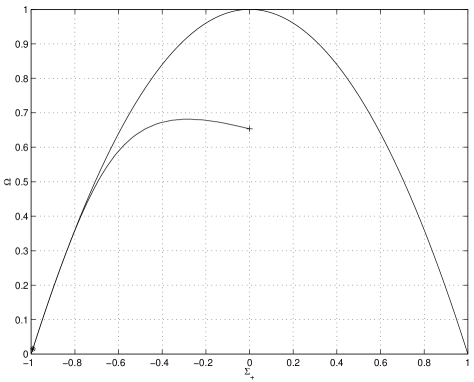
Figure 5. Part of a Taub type IX solution projected to the $\Sigma_{+}\Omega$-plane.

1. Let us first assume $\Sigma_{+}(\tau_{0})\leq 0$, $\Omega(\tau_{0})<1$ and $\Omega(\tau_{0})+\Sigma_{+}^{2}(\tau_{0})\geq 1$. Consider

$$\mathcal{C}=\{\tau\leq\tau_{0}:t\in[\tau,\tau_{0}]\Rightarrow\Sigma_{+}(t)\leq 0,\ \Omega(t)\leq\Omega(\tau_{0}),\ \Omega(t)+\Sigma_{+}^{2}(t)\geq 1\}.$$

We prove that $\mathcal{C}$ is not bounded from below. Assume the contrary. Let $t$ be the infimum of $\mathcal{C}$, which exists since $\mathcal{C}$ is non-empty and bounded from below. Since $t\in\mathcal{C}$, $\Sigma_{+}(t)<0$. Let $t^{\prime}<t$ be such that $\Sigma_{+}<0$ in $[t^{\prime},t]$. Observe that

(11.1) $$\Omega^{\prime}=[(3\gamma-2)(\Omega+\Sigma_{+}^{2}-1)+3(2-\gamma)\Sigma_{+}^{2}]\Omega.$$

By the constraint,

(11.2) $$\Omega+\Sigma_{+}^{2}-1=\frac{3}{4}N_{1}^{2}(4\frac{N_{2}}{N_{1}}-1).$$

Since $\Sigma_{+}<0$ in $[t^{\prime},t]$, $N_{2}/N_{1}$ increases as we go backward in that interval, because of

$$(\frac{N_{2}}{N_{1}})^{\prime}=6\Sigma_{+}\frac{N_{2}}{N_{1}}.$$

Consequently $\Omega+\Sigma_{+}^{2}\geq 1$ in $[t^{\prime},t]$, by (11.2), so that $\Omega$ decreases in the interval by (11.1). Thus $t^{\prime}\in\mathcal{C}$, contradicting the fact that $t$ is the infimum of $\mathcal{C}$.

Let $\tau\leq\tau_{0}$. Then $\Sigma_{+}(\tau)\leq-\sqrt{1-\Omega(\tau_{0})}$. By (11.1), we then conclude $\Omega\rightarrow 0$. By (2.1), we also conclude that $N_{1}N_{2}\rightarrow 0$ and $N_{1}\rightarrow 0$. By (11.2), we have $\Sigma_{+}\rightarrow-1$. Using the constraint (11.2) and (2.2), we conclude that $q+2\Sigma_{+}$ is integrable, so that $N_{2}=N_{3}$ will converge to a finite non-zero value.

2. Assume now $\Sigma_{+}(\tau_{0})\leq 0$, $\Omega(\tau_{0})<1$ and $\Omega(\tau_{0})+\Sigma_{+}^{2}(\tau_{0})<1$. Observe that

(11.3) $$\Sigma_{+}^{\prime}=(1-\Omega-\Sigma_{+}^{2})(4-2\Sigma_{+})-\frac{3}{2}(2-\gamma)\Omega\Sigma_{+}+9N_{1}N_{2}.$$

As long as $\Omega+\Sigma_{+}^{2}<1$, $\Sigma_{+}$ decreases as we go backward in time by (11.3). Then $N_{2}/N_{1}$ will increase exponentially until $\Omega+\Sigma_{+}^{2}=1$, by the constraint, and $\Sigma_{+}<0$. $\Box$

Lemma 11.2.

Consider a type IX solution with $\Sigma_{-}=0$, $N_{2}=N_{3}$ and $2/3<\gamma<2$. It is contained in a compact set for $\tau\leq 0$ and $N_{1}N_{2}\rightarrow 0$.

Proof. Note that $N_{1}$ must be bounded for $\tau\leq 0$, as follows from Lemma 3.3, the fact that $N_{2}=N_{3}$, and the fact that $N_{1}N_{2}N_{3}$ decreases backward in time. To prove the first statement, assume the contrary. Then there is a sequence $\tau_{k}\rightarrow-\infty$ such that $N_{2}(\tau_{k})\rightarrow\infty$. We can assume $N_{2}^{\prime}(\tau_{k})\leq 0$, and thus

(11.4) $$\frac{1}{2}(3\gamma-2)\Omega+2\Sigma_{+}^{2}+2\Sigma_{+}\leq 0$$

in $\tau_{k}$. Since $N_{1}N_{2}^{2}$ is decreasing as we go backward, $N_{1}$ and $N_{1}N_{2}$ evaluated at $\tau_{k}$ must go to zero. Thus $\Omega+\Sigma_{+}^{2}-1$ will become arbitrarily small in $\tau_{k}$ by (11.2). If $\Omega(\tau_{k})\geq 1$ for all $k$, we get

$$\Sigma_{+}(\tau_{k})\leq-\frac{1}{4}(3\gamma-2)$$

by (11.4), so that

$$\Sigma_{+}^{2}(\tau_{k})+\Omega(\tau_{k})\geq 1+\frac{1}{16}(3\gamma-2)^{2},$$

which is a contradiction. In other words, there is a $k$ such that $\Sigma_{+}(\tau_{k})\leq 0$, by (11.4), and $\Omega(\tau_{k})<1$. We can then use Lemma 11.1 to arrive at a contradiction to the assumption that the solution is not contained in a compact set.

To prove the second part of the lemma, observe that $N_{1}N_{2}^{2}$ converges to zero, as follows from the existence of an $\alpha$- limit point and Lemma 5.2. Thus

$$N_{1}N_{2}=N_{1}^{1/2}[N_{1}N_{2}^{2}]^{1/2}\leq C[N_{1}N_{2}^{2}]^{1/2}\rightarrow 0.$$

$\Box$

Proposition 11.1.

For a type IX solution with $\Sigma_{-}=0$, $N_{2}=N_{3}$ and $2/3<\gamma<2$, either the solution is contained in $\mathcal{F}_{\mathrm{IX}}$ or $\mathcal{P}_{\mathrm{IX}}$, or

$$\lim_{\tau\rightarrow-\infty}(\Omega,\Sigma_{+},\Sigma_{-},N_{1},N_{2},N_{3})(\tau)=(0,-1,0,0,n_{2},n_{2})$$

where $0<n_{2}<\infty$.

Remark. Compare with Proposition 3.1. Observe also that when $\Sigma_{+}$ for the solution converges to $-1$, we approach $\Sigma_{+}=-1,\ \Omega=0$ from outside the parabola $\Omega+\Sigma_{+}^{2}=1$, as follows from the proof of Lemma 11.1.

Proof. Consider a solution which is not contained in $\mathcal{F}_{\mathrm{IX}}$ or $\mathcal{P}_{\mathrm{IX}}$. By Lemma 11.2, there is an $\alpha$-limit point with $N_{1}N_{2}=0$. We can assume it is not $P_{1}^{+}(II)$. We have the following possibilities.

1. It is contained in $\mathcal{F}_{\mathrm{I}}\cup\mathcal{F}_{\mathrm{II}}\cup\mathcal{F}_{\mathrm{VII}_{0}}$. Then $F$ is an $\alpha$-limit point. Since the solution is not contained in $\mathcal{F}_{\mathrm{IX}}$, we get a type I limit point which is not $F$, by Lemma 4.2, and thus either $\Sigma_{+}=-1$ or $\Sigma_{+}=1$ as limit points, by Proposition 8.1. The first alternative implies convergence to $\Sigma_{+}=-1$, by Lemma 11.1. If we have a type I $\alpha$-limit point with $\Sigma_{+}=1$, we can apply the Kasner map by Proposition 6.1 in order to obtain a type I limit point with $\Sigma_{+}=-1$.

2. The limit point is of type I. This possibility can be dealt with as above.

3. It is of type II. We can assume that it is not $P_{1}^{+}(II)$, by Lemma 4.1, and that it is not contained in $\mathcal{F}_{\mathrm{II}}$. Thus we get $\Sigma_{+}=-1$ on the Kasner circle as an $\alpha$-limit point, by Proposition 9.1, and thus as above convergence to $\Sigma_{+}=-1$.

4. The limit point is of type VI$I_{0}$. We can assume $\Sigma_{+}\neq 0$. If $\Sigma_{+}<0$, we can apply Lemma 11.1 again, and if $\Sigma_{+}>0$, we get $\Sigma_{+}=1$ on the Kasner circle as an $\alpha$-limit point, by Proposition 10.1, a case which can be dealt with as above. $\Box$

12. Oscillatory behaviour

It will be necessary to consider Bianchi IX solutions to (2.1)-(2.3) under circumstances such that the behaviour is oscillatory. This section provides the technical tools needed.

Let $g$ be a function,

(12.1) $$A=\left(\begin{array}[]{rr}0&g\\ -g&0\end{array}\right),$$

and $\tilde{\mathbf{x}}=(\tilde{x},\tilde{y})^{t}$ satisfy

$$\tilde{\mathbf{x}}^{\prime}=A\tilde{\mathbf{x}}+\epsilon,$$

where $\epsilon$ is some vector valued function.

Lemma 12.1.

Let $\phi_{0}$ be such that $(\sin(\phi_{0}),\cos(\phi_{0}))$ and $(\tilde{x}(\tau_{0}),\tilde{y}(\tau_{0}))$ are parallel. Define

(12.2) $$\xi(\tau)=\int_{\tau_{0}}^{\tau}g(s)ds+\phi_{0}$$

and

(12.3) $$\mathbf{x}(\tau)=\left(\begin{array}[]{c}x(\tau)\\ y(\tau)\end{array}\right)=\left(\begin{array}[]{c}\sin\xi(\tau)\\ \cos\xi(\tau)\end{array}\right).$$

Then

(12.4) $$\|\tilde{\mathbf{x}}(\tau)-\mathbf{x}(\tau)\|\leq|1-(\tilde{x}^{2}(\tau_{0})+\tilde{y}^{2}(\tau_{0}))^{1/2}|+|\int_{\tau_{0}}^{\tau}\|\epsilon(s)\|ds|.$$

Proof. Let

$$\Phi=\left(\begin{array}[]{rr}y&-x\\ x&y\end{array}\right).$$

We have $[A,\Phi]=0$, $\Phi^{\prime}=-A\Phi$ and $\mathbf{x}^{\prime}=A\mathbf{x}$. We get

$$(\Phi(\tilde{\mathbf{x}}-\mathbf{x}))^{\prime}=-A\Phi(\tilde{\mathbf{x}}-\mathbf{x})+\Phi(A(\tilde{\mathbf{x}}-\mathbf{x})+\epsilon)=\Phi\epsilon.$$

Thus

$$(\tilde{\mathbf{x}}-\mathbf{x})(\tau)=\Phi^{-1}(\tau)\Phi(\tau_{0})(\tilde{\mathbf{x}}-\mathbf{x})(\tau_{0})+\Phi^{-1}(\tau)\int_{\tau_{0}}^{\tau}\Phi(s)\epsilon(s)ds.$$

But $\Phi$ takes values in $SO(2)$ and the lemma follows. $\Box$

In order to prove the existence of an $\alpha$-limit point for Bianchi IX solutions, and that, generically, there is a limit point on the Kasner circle, we need the following lemma.

Lemma 12.2.

Consider a Bianchi IX solution with $2/3<\gamma<2$. Assume there is a sequence $\tau_{k}\rightarrow-\infty$ such that $q(\tau_{k})\rightarrow 0$, and $N_{2}(\tau_{k}),\ N_{3}(\tau_{k})\rightarrow\infty$, then for each $T$, there is a $\tau\leq T$ such that $\Sigma_{+}(\tau)\geq 0$.

Proof. Observe that by (2.4), $q=0$ and $N_{2}+N_{3}\geq N_{1}$ implies $\Sigma_{+}^{\prime}\leq-2$. However, the only term appearing in the constraint which does not go to zero in $\tau_{k}$ is $(N_{2}-N_{3})^{2}$, since the product $N_{1}N_{2}N_{3}$ decreases as we go backward. Thus $|\Sigma_{-}^{\prime}(\tau_{k})|\rightarrow\infty$, and the behaviour is oscillatory. It is clear that $\Sigma_{+}^{\prime}$ could become positive during the oscillations, but only when $|\Sigma_{-}|$ is big, so that we on the whole should move in the positive direction.

Assume there is a $T$ such that $\Sigma_{+}(\tau)<0$ for all $\tau\leq T$.

We begin by examining the behaviour of different expressions in the sets

$$\mathcal{D}_{k}=\cup_{n=k}^{\infty}[\tau_{n}-1,\tau_{n}]$$

and

$$\mathcal{D}=\cup_{n=1}^{\infty}[\tau_{n}-1,\tau_{n}].$$

Observe that by the fact that $(\Omega,\Sigma_{+},\Sigma_{-})$ are constrained to belong to a compact set during $(-\infty,0]$, according to Lemma 3.3, $N_{2}$ and $N_{3}$ go to infinity uniformly in $\mathcal{D}$ (by which we will mean the following):

$$\forall M\ \exists K:k\geq K\Rightarrow N_{i}(\tau)\geq M\ \forall\tau\in\mathcal{D}_{k},\ i=2,3.$$

Thus $N_{1}$ and $N_{1}(N_{2}+N_{3})$ go to zero uniformly in $\mathcal{D}$. By (2.1), $\Omega$ also converges to zero uniformly in $\mathcal{D}$. Due to the constraint, we get a bound on $\Sigma_{-}^{2}+\frac{3}{4}(N_{2}-N_{3})^{2}$ in $\mathcal{D}$. Consider (2.4). The last two terms go to zero uniformly. If the first term is not negative, $1-\Omega-\Sigma_{+}^{2}-\Sigma_{-}^{2}\leq 0$. By the constraint, it will then be bounded by an expression that converges to zero uniformly in $\mathcal{D}$. Thus, for every $\delta>0$ there is a $K$ such that $k\geq K$ implies $\Sigma_{+}^{\prime}\leq\delta$ in $\mathcal{D}_{k}$. Combining this with the fact that $q(\tau_{k})\rightarrow 0$, and the assumption that $\Sigma_{+}(\tau)<0$ for $\tau\leq T$, we conclude that $\Sigma_{+}$ converges uniformly to zero in $\mathcal{D}$.

Next, we use Lemma 12.1 in order to approximate the oscillatory behaviour. Define the functions

$$\tilde{x} = \frac{\Sigma_{-}}{(1-\Sigma_{+}^{2})^{1/2}}$$

$$\tilde{y} = \frac{\sqrt{3}}{2}\frac{N_{2}-N_{3}}{(1-\Sigma_{+}^{2})^{1/2}}.$$

We can apply Lemma 12.1 with

$$g=-3(N_{2}+N_{3})-2(1+\Sigma_{+})\tilde{x}\tilde{y}=g_{1}+g_{2}$$

and $\epsilon_{x}$, $\epsilon_{y}$ given by (15.5) and (15.6), cf. Lemma 15.1. By the above, we conclude that $\tilde{x}$ and $\tilde{y}$ are uniformly bounded on $\mathcal{D}_{k}$, if $k$ is great enough, and that $\|\epsilon\|$ converges to zero uniformly on $\mathcal{D}$. Let $\mathbf{x}_{k}$ be the expression given by Lemma 12.1, with $\tau_{0}$ replaced by $\tau_{k}$ and $\phi_{0}$ by a suitable $\phi_{k}$. Let $\delta>0$. By the above and $q(\tau_{k})\rightarrow 0$, we get

(12.5) $$\|(\tilde{\mathbf{x}}-\mathbf{x}_{k})(\tau)\|\leq\delta,$$

if $\tau\in[\tau_{k}-1,\tau_{k}]$, and $k$ is great enough. In $[\tau_{k}-1,\tau_{k}]$, we thus have

(12.6) $$\Sigma_{+}^{\prime}=-2+2x_{k}^{2}(1-\Sigma_{+}^{2})+\rho_{k},$$

where the error $\rho_{k}$ can be assumed to be arbitrarily small by choosing $k$ great enough, cf. (2.4).

Let

$$\xi_{k}(\tau)=\int_{\tau_{k}}^{\tau}g(s)ds+\phi_{k}$$

be as in (12.2). Since $N_{2}+N_{3}$ goes to infinity uniformly, $[\tau_{k}-1,\tau_{k}]$ can be assumed to contain an arbitrary number of periods of $\xi_{k}$, if $k$ is great enough. Thus, we can assume the existence of $\tau_{1,k},\tau_{2,k}\in[\tau_{k}-1,\tau_{k}]$, such that $\tau_{2,k}-\tau_{1,k}\geq 1/2$ and $\xi_{k}(\tau_{1,k})-\xi_{k}(\tau_{2,k})$ is an integer multiple of $\pi$. Let $[\tau_{1},\tau_{2}]\subseteq[\tau_{1,k},\tau_{2,k}]$ satisfy $\xi_{k}(\tau_{1})-\xi_{k}(\tau_{2})=\pi$. We can assume $\tau_{2}-\tau_{1}$ to be arbitrarily small by choosing $k$ great enough. Considering (2.1), and using the fact that $q$ is bounded, we conclude that $N_{2}+N_{3}$ cannot change by more than a factor arbitrarily close to one during $[\tau_{1},\tau_{2}]$. Since the expression involving $N_{2}+N_{3}$ dominates $g$, we conclude that

$$-\frac{3}{4}g(\tau_{\mathrm{max}})\leq-g(\tau_{\mathrm{min}}),$$

where $\tau_{\mathrm{max}}$ and $\tau_{\mathrm{min}}$ correspond to the maximum and the minimum of $-g$ in $[\tau_{1},\tau_{2}]$. Estimate

$$\int_{\tau_{1}}^{\tau_{2}}2x_{k}^{2}(1-\Sigma_{+}^{2})ds=\int_{\xi_{k}(\tau_{1})}^{\xi_{k}(\tau_{2})}\frac{2x_{k}^{2}(1-\Sigma_{+}^{2})}{g}d\eta=-\int_{\xi_{k}(\tau_{1})-\pi}^{\xi_{k}(\tau_{1})}\frac{2x_{k}^{2}(1-\Sigma_{+}^{2})}{g}d\eta\leq$$

$$\leq-\frac{1}{g(\tau_{\mathrm{min}})}\int_{\xi_{k}(\tau_{1})-\pi}^{\xi_{k}(\tau_{1})}2\sin^{2}(\eta)d\eta=-\frac{\pi}{g(\tau_{\mathrm{min}})}.$$

We get

$$\tau_{2}-\tau_{1}=\int_{\xi_{k}(\tau_{1})}^{\xi_{k}(\tau_{2})}\frac{1}{g}d\eta\geq-\frac{\pi}{g(\tau_{\mathrm{max}})}\geq\frac{3}{4}\int_{\tau_{1}}^{\tau_{2}}2x_{k}^{2}(1-\Sigma_{+}^{2})ds.$$

Consequently, (12.6) yields

$$\Sigma_{+}(\tau_{2})-\Sigma_{+}(\tau_{1})=-2(\tau_{2}-\tau_{1})+\int_{\tau_{1}}^{\tau_{2}}2x_{k}^{2}(1-\Sigma_{+}^{2})ds+\int_{\tau_{1}}^{\tau_{2}}\rho_{k}d\tau\leq$$

$$\leq-\frac{2}{3}(\tau_{2}-\tau_{1})+\int_{\tau_{1}}^{\tau_{2}}\rho_{k}d\tau.$$

Since $\xi_{k}(\tau_{1,k})-\xi_{k}(\tau_{2,k})$ corresponds to an integer multiple of $\pi$, we conclude that

$$\Sigma_{+}(\tau_{2,k})-\Sigma_{+}(\tau_{1,k})\leq-\frac{2}{3}(\tau_{2,k}-\tau_{1,k})+\int_{\tau_{1,k}}^{\tau_{2,k}}\rho_{k}d\tau\leq-\frac{1}{3}+\int_{\tau_{1,k}}^{\tau_{2,k}}\rho_{k}d\tau.$$

However, the expressions on the far left can be assumed to be arbitrarily small, and the integral of $\rho_{k}$ can be assumed to be arbitrarily small. We have a contradiction. $\Box$

13. Bianchi IX solutions

We first prove that there is an $\alpha$-limit point. If we assume that there is no $\alpha$-limit point, we get the conclusion that the Euclidean norm $\|N\|$ of the vector $(N_{1},N_{2},N_{3})$ has to converge to infinity, since $(\Omega,\Sigma_{+},\Sigma_{-})$ is constrained to belong to a compact set to the past by Lemma 3.3. In fact, Lemma 3.3 yields more; it implies that two $N_{i}$ have to be large at any given time. Since the product $N_{1}N_{2}N_{3}$ decays as we go backward, the third $N_{i}$ has to be small. Sooner or later, the two $N_{i}$ which are large and the one which is small have to be fixed, since a ’changing of roles’ would require two $N_{i}$ to be small, and thereby also the third by Lemma 3.3, contradicting the fact that $\|N\|\rightarrow\infty$. Therefore, one can assume that two $N_{i}$ converge to infinity, and that the third converges to zero. More precisely we have.

Lemma 13.1.

Consider a Bianchi IX solution. If $\|N\|\rightarrow\infty$, we can, by applying the symmetries to the equations, assume that $N_{2},\ N_{3}\rightarrow\infty$ and $N_{1},\ N_{1}(N_{2}+N_{3})\rightarrow 0$.

Proof. As in the vacuum case, see [16]. $\Box$

Lemma 13.2.

A Bianchi IX solution with $2/3<\gamma<2$ has an $\alpha$-limit point.

Proof. If the solution is of Taub type, we already know that it is true so assume not. We assume $N_{2},\ N_{3}\rightarrow\infty$, since if this does not occur, there is an $\alpha$-limit point by Lemma 3.3 and Lemma 13.1. By (2.4) we have $\Sigma_{+}^{\prime}<0$ if $\Sigma_{+}=0$ using the constraint (assuming $N_{2}+N_{3}>3N_{1}$). Thus, there is a $T$ such that if $\Sigma_{+}$ attains zero in $\tau\leq T$, it will be non-negative to the past, and thus $N_{2}N_{3}$ will be bounded to the past since $\Sigma_{+}$ has to be negative for the product to grow. If there is a sequence $\tau_{k}\rightarrow-\infty$ such that $q(\tau_{k})\rightarrow 0$, we can apply Lemma 12.2 to arrive at a contradiction. Thus there is an $S$ such that

(13.1) $$q(\tau)\geq\epsilon>0$$

for all $\tau\leq S$.

Consider

(13.2) $$Z_{-1}=\frac{\frac{4}{3}\Sigma_{-}^{2}+(N_{2}-N_{3})^{2}}{N_{2}N_{3}}.$$

The reason we consider this function is that the derivative is in a sense almost negative, so that it almost increases as we go backward. On the other hand, it converges to zero as $\tau\rightarrow-\infty$ by our assumptions. The lemma follows from the resulting contradiction. We have

(13.3) $$Z_{-1}^{\prime}=\frac{h}{N_{2}N_{3}}=\frac{-\frac{16}{3}\Sigma_{-}^{2}(1+\Sigma_{+})+4\sqrt{3}\Sigma_{-}(N_{2}-N_{3})N_{1}}{N_{2}N_{3}}.$$

Letting

$$f=\frac{4}{3}\Sigma_{-}^{2}+(N_{2}-N_{3})^{2},$$

we have, using the constraint,

$$h\leq 4\Sigma_{-}^{2}N_{1}(N_{2}+N_{3})+2\sqrt{3}N_{1}f\leq N_{1}N_{2}N_{3}f$$

for, say, $\tau\leq T^{\prime}\leq S$. Thus

(13.4) $$Z_{-1}^{\prime}\leq N_{1}N_{2}N_{3}Z_{-1}$$

for all $\tau\leq T^{\prime}$. Since $q\geq\epsilon>0$ for all $\tau\leq T^{\prime}\leq S$ by (13.1), we get

$$(N_{1}N_{2}N_{3})(\tau)\leq(N_{1}N_{2}N_{3})(T^{\prime})\exp[3\epsilon(\tau-T^{\prime})]$$

for $\tau\leq T^{\prime}$. Inserting this inequality in (13.4) we can integrate to obtain

$$Z_{-1}(\tau)\geq Z_{-1}(T^{\prime})\exp(-\frac{1}{3\epsilon}(N_{1}N_{2}N_{3})(T^{\prime}))>0$$

for $\tau\leq T^{\prime}$. But $Z_{-1}(\tau)\rightarrow 0$ as $\tau\rightarrow-\infty$ by our assumption, and we have a contradiction. $\Box$

Corollary 13.1.

Consider a Bianchi IX solution with $2/3<\gamma<2$. For all $\epsilon>0$, there is a $T$ such that

$$\Omega+\Sigma_{+}^{2}+\Sigma_{-}^{2}\leq 1+\epsilon$$

for all $\tau\leq T$. Furthermore

$$\lim_{\tau\rightarrow-\infty}(N_{1}N_{2}N_{3})(\tau)=0.$$

Proof. As in the vacuum case, see [16]. The second part follows from Lemma 5.2 and Lemma 13.2. $\Box$

Proposition 13.1.

A generic Bianchi IX solution with $2/3<\gamma<2$ has an $\alpha$-limit point on the Kasner circle.

Proof. Observe that by Lemma 13.2 and Corollary 13.1, there is an $\alpha$-limit point of type I, II or VI$\mathrm{I}_{0}$.

1. First we prove that we can assume the $\alpha$-limit point to be a type VI$I_{0}$ point with $N_{1}=0,\ 0<N_{2}=N_{3},\ \Omega=0,\ \Sigma_{-}=0$ and $\Sigma_{+}=-1$.

a. If there is an $\alpha$-limit point in $\mathcal{F}_{\mathrm{I}}$, $\mathcal{F}_{\mathrm{II}}$ or $\mathcal{F}_{\mathrm{VII}_{0}}$, $F$ is a limit point, but then there is an $\alpha$-limit point on the Kasner circle, by Lemma 4.2 and Proposition 8.1.

b. Assume there is an $\alpha$-limit point in $\mathcal{P}_{\mathrm{VII}_{0}}$, or that one of $P_{i}^{+}(II)$ is an $\alpha$-limit point. Then there is a limit point of type II which is not $P_{i}^{+}(II)$, by Lemma 4.1, and we can assume it does not belong to $\mathcal{F}_{\mathrm{II}}$. We thus get an $\alpha$-limit point on the Kasner circle by Proposition 9.1.

c. Consider the complement of the above. We have an $\alpha$-limit point of type I, II or VI$\mathrm{I}_{0}$ which is generic or possibly of Taub type. If the limit point is of type I or II, we get an $\alpha$-limit point on the Kasner circle by Proposition 8.1 and Proposition 9.1. If the limit point is a non-Taub type VI$\mathrm{I}_{0}$ point, we get an $\alpha$-limit point on the Kasner circle by Proposition 10.2. Assume it is of Taub type with $\Sigma_{-}=0$, $N_{2}=N_{3}$. By Proposition 10.1, we can assume that we have an $\alpha$-limit point of the type mentioned.

2. We construct an $\alpha$-limit point on the Kasner circle given an $\alpha$-limit point as in 1. Since the solution is not of Taub type, we must leave a neighbourhood of the point $(\Sigma_{+},\Sigma_{-})=(-1,0)$. If $N_{2}$ and $N_{3}$ evaluated at the times we leave do not go to infinity, we are done. The reason is that we can choose the neighbourhood to be so small that $\Omega$ and $N_{1}$ decrease exponentially in it, see (2.1). If $N_{2}(t_{k})$ or $N_{3}(t_{k})$ is bounded, we get a vacuum Bianchi VI$\mathrm{I}_{0}$ $\alpha$-limit point which is not of Taub-type by choosing a suitable subsequence (if we get a type I or II point we are done, see the above arguments). By Proposition 10.2, we then get an $\alpha$-limit point on the Kasner circle. Thus, we can assume the existence of a sequence $t_{k}\rightarrow-\infty$ such that $N_{2}(t_{k})$ and $N_{3}(t_{k})$ go to infinity.

There are two problems we have to confront. First of all $N_{2}$ and $N_{3}$ have to decay from their values in $t_{k}$ in order for us to get an $\alpha$-limit point. Secondly, and more importantly, we need to see to it that we do not get an $\alpha$-limit point of the same type we started with. Let us divide the situation into two cases.

a. Assume that for each $t_{k}$ there is an $s_{k}\leq t_{k}$ such that $\Sigma_{+}(s_{k})=0$. Observe that when $\Sigma_{+}=0$, we have

$$\Sigma_{+}^{\prime}\leq\frac{1}{2}N_{1}(9N_{1}-3N_{2}-3N_{3})$$

by the constraint (2.3), and (2.4). Thus, we can assume that we have $3N_{1}\geq N_{2}+N_{3}$ in $s_{k}$, since there is an $\alpha$-limit point with $\Sigma_{+}=-1$. Thus there must be an $r_{k}\leq t_{k}$ such that, at $r_{k}$, either $N_{1}=N_{2}<N_{3}$, $N_{1}=N_{3}<N_{2}$ or $N_{1}<N_{2}$, $N_{1}<N_{3}$ and $3N_{1}\geq N_{2}+N_{3}$. One of these possibilities must occur an infinite number of times. The first two possibilities yield a type I or II limit point, and the last a type I limit point because, of the fact that $N_{1}N_{2}N_{3}\rightarrow 0$ and Lemma 3.3. As above, we get an $\alpha$-limit point on the Kasner circle.

b. Assume there is a $T$ such that $\Sigma_{+}(\tau)<0$ for all $\tau\leq T$. Then $N_{1}\rightarrow 0$, since $N_{1}(t_{k})\rightarrow 0$, and $\Sigma_{+}<0$ implies that $N_{1}$ is monotone. Assume there is a sequence $\tau_{k}\rightarrow-\infty$ such that $N_{2}$ or $N_{3}$ evaluated at it goes to zero. Then we get an $\alpha$ limit point of type I or II, a situation we may deal with as above. Thus we may assume $N_{i}\geq\epsilon>0$, $i=2,3$ to the past of $T$. Similarly to the proof of the existence of an $\alpha$-limit point, we have

$$Z_{-1}^{\prime}\leq c_{\epsilon}N_{1}N_{2}N_{3}Z_{-1}.$$

If there is an $S$ and a $\xi>0$ such that $q(\tau)\geq\xi>0$ for all $\tau\leq S$, we get a contradiction as in the proof of Lemma 13.2, since $(N_{2}N_{3})(t_{k})\rightarrow\infty$. Thus there exists a sequence $\tau_{k}\rightarrow-\infty$ such that $q(\tau_{k})\rightarrow 0$. If $N_{2}(\tau_{k})$ or $N_{3}(\tau_{k})$ contains a bounded subsequence, we may refer to possibilities already handled. By Lemma 12.2, we get $\Sigma_{+}\geq 0$, a contradiction. $\Box$

14. Control over the density parameter

The idea behind the main argument is to use the existence of an $\alpha$-limit point on the Kasner circle to obtain a contradiction to the assumption that the solution does not converge to the closure of the set of vacuum type II points. The function

$$d=\Omega+N_{1}N_{2}+N_{2}N_{3}+N_{3}N_{1}$$

is a measure of the distance from the attractor. We can consider $d$ to be a function of $\tau$, if we evaluate it at a generic Bianchi IX solution. If $\tau_{k}\rightarrow-\infty$ yields the $\alpha$-limit point on the Kasner circle, then $d(\tau_{k})\rightarrow 0$. If $d$ does not converge to zero, then it must grow from an arbitrarily small value up to some fixed number, say $\delta>0$, as we go backward. In the contradiction argument, it is convenient to know that the growth occurs only in the sum of products of the $N_{i}$, and that during the growth one can assume $\Omega$ to be arbitrarily small. The following proposition achieves this goal, assuming $\delta$ is small enough, which is not a restriction. The proof is to be found at the end of this section.

Proposition 14.1.

Consider a Bianchi IX solution with $2/3<\gamma<2$. There exists an $\epsilon>0$ such that if

(14.1) $$N_{1}N_{2}+N_{2}N_{3}+N_{1}N_{3}\leq\epsilon$$

in $[\tau_{1},\tau_{2}]$, then

$$\Omega\leq c_{\gamma}\Omega(\tau_{2})$$

in $[\tau_{1},\tau_{2}]$ if $\Omega(\tau_{2})\leq\epsilon$. Here $c_{\gamma}>0$ only depends on $\gamma$.

The idea of the proof is the following. If the sum of product of the $N_{i}$ and $\Omega$ are small, the solution should behave in the following way. If all the $N_{i}$ are small, then we are close to the Kasner circle and $\Omega$ decays exponentially. One of the $N_{i}$ may become large alone, and then $\Omega$ increases, but it can only be large for a short period of time. After that it must decay until some other $N_{i}$ becomes large. But this process of the $N_{i}$ changing roles takes a long time, and most of it occurs close to the Kasner circle, where $\Omega$ decays exponentially. Thus, $\Omega$ may increase by a certain factor, but after that it must decay by a larger factor until it can increase again, hence the result. Figure 6 illustrates the behaviour.

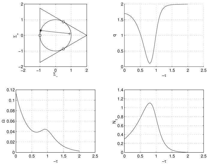
Figure 6. Part of a type IX solution.

We divide the proof into lemmas, and begin by making the statement that $\Omega$ decays exponentially close to the Kasner circle more precise.

Lemma 14.1.

Consider a Bianchi IX solution with $2/3<\gamma<2$. If

$$\Sigma_{+}^{2}+\Sigma_{-}^{2}\geq\frac{1}{8}(3\gamma+2)$$

in an interval $[s_{1},s_{2}]$, then

$$\Omega(s)\leq\Omega(s_{2})e^{-\alpha_{\gamma}(s_{2}-s)}$$

for $s\in[s_{1},s_{2}]$, where

$$\alpha_{\gamma}=\frac{3}{2}(2-\gamma).$$

Proof. Observe that

(14.2) $$\Omega^{\prime}\geq 4[\Sigma_{+}^{2}+\Sigma_{-}^{2}-\frac{1}{4}(3\gamma-2)]\Omega,$$

so that under the conditions of the lemma

$$\Omega^{\prime}\geq\alpha_{\gamma}\Omega.$$

The conclusion follows. $\Box$

Next, we prove that if the $N_{i}$ all stay sufficiently small under a condition as in (14.1) and $\Omega$ starts out small, then $\Omega$ will remain small.

Lemma 14.2.

Consider a Bianchi IX solution with $2/3<\gamma<2$. There is an $\epsilon>0$ such that if

(14.3) $$\frac{3}{4}N_{i}^{2}\leq\frac{1}{8}(6-3\gamma)$$

(14.4) $$N_{1}N_{2}+N_{2}N_{3}+N_{1}N_{3}\leq\epsilon$$

in an interval $[s_{1},s_{2}]$, and $\Omega(s_{2})\leq\epsilon$, then $\Omega(s)\leq\Omega(s_{2})$ for all $s\in[s_{1},s_{2}]$.

Proof. Let

$$\mathcal{E}=\{\tau\in[s_{1},s_{2}]:t\in[\tau,s_{2}]\Rightarrow\Omega(t)\leq\Omega(s_{2})\}.$$

Let $\tau\in\mathcal{E}$, $\tau>s_{1}$. There must be two $N_{i}$, say $N_{2}$ and $N_{3}$, such that $N_{2}\leq\epsilon^{1/2}$ and $N_{3}\leq\epsilon^{1/2}$ in $\tau$, by (14.4). By the constraint (2.3) and (14.4), we have in $\tau$,

$$\Sigma_{+}^{2}+\Sigma_{-}^{2}\geq 1-\frac{3}{4}N_{1}^{2}-\Omega-h_{1}\geq\frac{1}{8}(3\gamma+2)-4\epsilon,$$

so that assuming $\epsilon$ small enough depending only on $\gamma$, we have $\Omega^{\prime}(\tau)>0$, cf. (14.2). Thus there exists an $s<\tau$ such that $s\in\mathcal{E}$. In other words, $\mathcal{E}$ is an open, closed, and non-empty subset of $[s_{1},s_{2}]$, so that $\mathcal{E}=[s_{1},s_{2}]$. $\Box$

The next lemma describes the phase during which $\Omega$ may increase.

Lemma 14.3.

Consider a Bianchi IX solution with $2/3<\gamma<2$. There is an $\epsilon>0$ such that if

(14.5) $$\frac{3}{4}N_{1}^{2}\geq\frac{1}{8}(6-3\gamma)$$

(14.6) $$N_{1}N_{2}+N_{2}N_{3}+N_{1}N_{3}\leq\epsilon$$

in $[s_{1},s_{2}]$, and $\Omega(s_{2})\leq\epsilon$, then $s_{2}-s_{1}\leq c_{1,\gamma}$ and $\Omega(s)\leq c_{2,\gamma}\Omega(s_{2})$ for all $s\in[s_{1},s_{2}]$, where $c_{1,\gamma}$ and $c_{2,\gamma}$ are positive constants depending on $\gamma$.

Proof. Assume $\epsilon$ is small enough that

$$\frac{3}{4}\epsilon^{1/2}\leq\frac{1}{8}(6-3\gamma),$$

so that $N_{1}\geq\epsilon^{1/4}$ in $[s_{1},s_{2}]$. Assuming $\epsilon<1$ we get $N_{i}\leq\epsilon^{1/2}$ in $[s_{1},s_{2}]$, $i=2,3$. Use the constraint (2.3) to write

(14.7) $$1-\Omega-\Sigma_{+}^{2}-\Sigma_{-}^{2}=\frac{3}{4}N_{1}^{2}+h_{1}$$

where $|h_{1}|\leq 3\epsilon$ by (14.6). Thus,

$$1-\Omega-\Sigma_{+}^{2}-\Sigma_{-}^{2}\geq\frac{3}{4}\epsilon^{1/2}-3\epsilon,$$

so that we may assume

(14.8) $$\Omega+\Sigma_{+}^{2}+\Sigma_{-}^{2}<1$$

in $[s_{1},s_{2}]$.

We now compare the behaviour with a type II vacuum solution. By (2.4) and (14.7), we have

(14.9) $$\Sigma_{+}^{\prime}=-2(\frac{3}{4}N_{1}^{2}+h_{1})(\Sigma_{+}+1)-\frac{3}{2}(2-\gamma)\Omega\Sigma_{+}+\frac{9}{2}N_{1}^{2}-$$

$$-\frac{9}{2}N_{1}(N_{2}+N_{3})=\frac{3}{2}N_{1}^{2}(2-\Sigma_{+})+h_{2}\Omega+h_{3},$$

where $|h_{3}|\leq 17\epsilon$ and $|h_{2}|\leq 2$ in $[s_{1},s_{2}]$. Let $a_{\gamma}=(6-3\gamma)/4$. Then,

$$\Sigma_{+}(s_{2})-\Sigma_{+}(s_{1})\geq a_{\gamma}(s_{2}-s_{1})+\int_{s_{1}}^{s_{2}}(h_{2}\Omega+h_{3})dt.$$

However,

$$\Omega(s)\leq\Omega(s_{2})e^{-4(s-s_{2})}\leq\epsilon e^{-4(s-s_{2})}$$

for all $s\in[s_{1},s_{2}]$, see (2.1). Thus,

$$|\int_{s_{1}}^{s_{2}}h_{2}\Omega ds|\leq\frac{1}{2}\Omega(s_{2})e^{4(s_{2}-s_{1})}.$$

We get

$$\Sigma_{+}(s_{2})-\Sigma_{+}(s_{1})\geq a_{\gamma}(s_{2}-s_{1})-\frac{1}{2}\epsilon e^{4(s_{2}-s_{1})}-17\epsilon(s_{2}-s_{1}).$$

This inequality contradicts the statement that $s_{2}-s_{1}$ may be taken equal to $4/a_{\gamma}$, by choosing $\epsilon$ small enough. We conclude that $s_{2}-s_{1}\leq 4/a_{\gamma}=c_{1,\gamma}$, and that we may choose $c_{2,\gamma}=\exp(16/a_{\gamma})$. $\Box$

The following lemma deals with the decay in $\Omega$ that has to follow an increase. The idea is that if $N_{1}$ is on the boundary between big and small, and its derivative is non-negative at a point, then it will decrease as we go backward, and the solution will not move far from the Kasner circle until one of the other $N_{i}$ has become large. That takes a long time and $\Omega$ will decay.

Lemma 14.4.

Consider a Bianchi IX solution such that $2/3<\gamma<2$. There is an $\epsilon>0$ such that if

(14.10) $$N_{1}N_{2}+N_{2}N_{3}+N_{3}N_{1}\leq\epsilon$$

in $[s_{1},s_{2}]$,

$$\frac{3}{4}N_{1}^{2}(s_{2})=\frac{1}{8}(6-3\gamma),\ N_{1}^{\prime}(s_{2})\geq 0$$

and $\Omega(s_{2})\leq c_{2,\gamma}\epsilon$, where $c_{2,\gamma}$ is the constant appearing in Lemma 14.3, then $\Omega$ decays as we go backward starting at $s_{2}$, until $s=s_{1}$, or we reach a point $s$ at which

$$\Omega(s)\leq\frac{\Omega(s_{2})}{2c_{2,\gamma}}.$$

Proof. We begin by assuming that $\epsilon>0$ is a fixed number. As the proof progresses, we will restrict it to be smaller than a certain constant depending on $\gamma$. We could spell it out here, but prefer to add restrictions successively. Let $N_{1}\geq\epsilon^{1/4}$ in $[t_{1},s_{2}]$ and $N_{1}(t_{1})=\epsilon^{1/4}$ or $t_{1}=s_{1}$, in case $N_{1}$ does not attain $\epsilon^{1/4}$ in $[s_{1},s_{2}]$. As in the proof of Lemma 14.3, we conclude that $N_{i}\leq\epsilon^{1/2}$, $i=2,3$ in $[t_{1},s_{2}]$, and that we may assume

(14.11) $$\Omega+\Sigma_{+}^{2}+\Sigma_{-}^{2}<1.$$

The variables $(\Omega,\Sigma_{+},\Sigma_{-})$ have to belong to the interior of a paraboloid for $N_{1}^{\prime}$ to be negative. Since $N_{1}^{\prime}(s_{2})\geq 0$ we are on the boundary or outside the paraboloid. The boundary is given by $g=0$, where

$$g=\frac{1}{2}(3\gamma-2)\Omega+2\Sigma_{+}^{2}+2\Sigma_{-}^{2}-4\Sigma_{+}.$$

An outward pointing normal is given by $\nabla g$, where the derivatives are taken in the order: $\Omega$, $\Sigma_{+}$ and $\Sigma_{-}$. Let

$$\mathcal{E}=\{\tau\in[t_{1},s_{2}]:t\in[\tau,s_{2}]\Rightarrow N_{1}^{\prime}(t)\geq 0,\ \Omega(t)\leq c_{2,\gamma}\epsilon\}.$$

Let $\tau\in\mathcal{E}$. By (14.11) we get $q(\tau)<2$ and, as we are also outside the interior of the paraboloid, $\Sigma_{+}(\tau)\leq 1/2$. For $\epsilon$, and thereby $\Omega$, small enough depending only on $\gamma$, we have

$$\Sigma_{+}^{\prime}(\tau)\geq\epsilon^{1/2},$$

cf. (14.9). Using the above observations, we estimate in $\tau$,

$$\nabla g\cdot(\Omega^{\prime},\Sigma_{+}^{\prime},\Sigma_{-}^{\prime})\leq C_{\gamma}\epsilon-\epsilon^{1/2},$$

where $C_{\gamma}$ only depends on $\gamma$. For $\epsilon$ small enough, the scalar product is negative. Thus, if $(\Omega(\tau),\Sigma_{+}(\tau),\Sigma_{-}(\tau))$ is on the surface of the paraboloid, the solution moves away from it as we go backward, so that $N_{1}^{\prime}\geq 0$ in $[s,\tau]$ for some $s<\tau$. If we are already outside the paraboloid, the existence of such an $s$ is guaranteed by less complicated arguments. As in the proof of Lemma 14.2, we get $\Omega^{\prime}>0$ for $\epsilon$ small enough depending only on $\gamma$, so that $\mathcal{E}$ is open, closed and non-empty. Thus $N_{1}$ decreases from $s_{2}$ to $t_{1}$ going backward. Now,

$$\Sigma_{+}^{2}+\Sigma_{-}^{2}\geq 1-\frac{3}{4}N_{1}^{2}-\Omega-h_{1}\geq\frac{1}{8}(3\gamma+2)-c_{2,\gamma}\epsilon-3\epsilon$$

in $[t_{1},s_{2}]$, so that

(14.12) $$\Omega(t_{1})\leq\Omega(s_{2})e^{-(2-\gamma)(s_{2}-t_{1})},$$

by an argument similar to Lemma 14.1, if $\epsilon$ is small enough. We can assume $\epsilon$ is small enough that the time required for $N_{1}$ to decrease to $\epsilon^{1/4}$ is great enough that if $t_{1}\neq s_{1}$, then the conclusion of the lemma follows by (14.12). $\Box$

Proof of Proposition 14.1. Assume $\epsilon$ is small enough that all the conditions of Lemma 14.2-14.4 are fulfilled. We divide the interval $[\tau_{1},\tau_{2}]$ into suitable subintervals, such that we may apply the above lemmas to them. If

(14.13) $$\frac{3}{4}N_{i}^{2}\leq\frac{1}{8}(6-3\gamma)$$

in $\tau_{2}$ for $i=1,2,3$, then we let $t_{2}\in[\tau_{1},\tau_{2}]$ be the smallest member of the interval such that (14.13) holds in all of $[t_{2},\tau_{2}]$. Otherwise, we chose $t_{2}=\tau_{2}$. Either $t_{2}=\tau_{1}$ or $3N_{1}^{2}(t_{2})/4\geq(6-3\gamma)/8$, by a suitable permutation of the variables. If $t_{2}\neq\tau_{1}$, let $t_{1}$ be the smallest member of $[\tau_{1},t_{2}]$ such that $3N_{1}^{2}/4\geq(6-3\gamma)/8$ in $[t_{1},t_{2}]$.

Because of Lemma 14.2, $\Omega$ decays in $[t_{2},\tau_{2}]$. If $t_{2}=\tau_{1}$, we are done; let $c_{\gamma}=1$. Otherwise, we apply Lemma 14.3 to the interval $[t_{1},t_{2}]$ to conclude that $\Omega(\tau)\leq c_{2,\gamma}\Omega(\tau_{2})$ in $[t_{1},\tau_{2}]$. If $t_{1}=\tau_{1}$, we can choose $c_{\gamma}=c_{2,\gamma}$. Otherwise, we apply Lemma 14.4 to $[\tau_{1},t_{1}]$. Either $\Omega$ decays until we have reached $\tau_{1}$, or there is a point $s_{1}\in[\tau_{1},t_{1}]$ such that $\Omega(s_{1})\leq\Omega(\tau_{2})/2$. By the proof of Lemma 14.4, we can assume that $\tau_{2}-s_{1}\geq 1$; some time has to elapse for the decay to take place.

Given an interval $[\tau_{1},\tau_{2}]$ as in the statement of the proposition, there are thus two possibilities. Either $\Omega(\tau)\leq c_{2,\gamma}\Omega(\tau_{2})$ for all $\tau\in[\tau_{1},\tau_{2}]$ or we can construct an $s_{1}\in[\tau_{1},\tau_{2}]$ such that $\tau_{2}-s_{1}\geq 1$, $\Omega(s_{1})\leq\Omega(\tau_{2})/2$, and $\Omega(\tau)\leq c_{2,\gamma}\Omega(\tau_{2})$ for all $\tau\in[s_{1},\tau_{2}]$. If the second possibility is the one that occurs, we can apply the same argument to $[\tau_{1},s_{1}]$, and by repeated application, the proposition follows. $\Box$

Corollary 14.1.

Consider a Bianchi IX solution with $2/3<\gamma<2$. If

$$\lim_{\tau\rightarrow-\infty}(N_{1}N_{2}+N_{2}N_{3}+N_{1}N_{3})=0$$

and there is a sequence $\tau_{k}\rightarrow-\infty$ such that $\Omega(\tau_{k})\rightarrow 0$, then

$$\lim_{\tau\rightarrow-\infty}\Omega(\tau)=0.$$

15. Generic attractor for Bianchi IX solutions

In this section, we prove that for a generic Bianchi IX solution, the closure of the set of type II vacuum points is an attractor, assuming $2/3<\gamma<2$. What we need to prove is that

$$\lim_{\tau\rightarrow-\infty}(\Omega+N_{1}N_{2}+N_{2}N_{3}+N_{1}N_{3})=0,$$

since then we may for each $\epsilon>0$ choose a $T$ such that at least two of the $N_{i}$ and $\Omega$ must be less than $\epsilon$ for $\tau\leq T$. The starting point is the existence of a limit point on the Kasner circle for a generic solution, given by Proposition 13.1. Since there is such a limit point, there is a sequence $\tau_{k}\rightarrow-\infty$ such that $N_{i}(\tau_{k})$ and $\Omega(\tau_{k})$ go to zero. If

(15.1) $$h=N_{1}N_{2}+N_{2}N_{3}+N_{1}N_{3}$$

does not converge to zero, it must thus grow from an arbitrarily small value up to some $\epsilon$. By choosing $\epsilon$ so that Proposition 14.1 is applicable, we have control over $\Omega$. A few arguments yield the conclusion that we may assume that it is the product $N_{2}N_{3}$ that grows, and that the growth occurs close to the special point $(\Sigma_{+},\Sigma_{-})=(-1,0)$. Close to this point, $\Omega$, $N_{1}$ and $N_{1}(N_{2}+N_{3})$ decay exponentially, so as far as intuition goes, we may equate them with zero. We thus have a Bianchi VI$\mathrm{I}_{0}$ vacuum solution close to the special point $(-1,0)$. The behaviour of $N_{2}N_{3}$ will be oscillatory, and we may reduce the problem to one in which the product behaves essentially as a sine wave. However, by doing some technical estimates, one may see that one goes down going from top to top during the oscillation, and that that contradicts the assumed growth. Figure 7 illustrates the behaviour. It is a simulation of part of a Bianchi VI$\mathrm{I}_{0}$ vacuum solution.

Figure 7. Part of a Bianchi VI$\mathrm{I}_{0}$ vacuum solution.

We begin by rewriting the solutions in a form that makes the oscillatory behaviour apparent. Consider a non Taub-NUT Bianchi IX solution in an interval such that $-1<\Sigma_{+}<1$. Define the functions

(15.2) $$\tilde{x} = \frac{\Sigma_{-}}{(1-\Sigma_{+}^{2})^{1/2}}$$

(15.3) $$\tilde{y} = \frac{\sqrt{3}}{2}\frac{N_{2}-N_{3}}{(1-\Sigma_{+}^{2})^{1/2}}.$$

The reason why these expressions are natural to consider is that, for reasons mentioned above, $N_{1}$, $\Omega$ and so forth may be considered to be zero. In the situation we will need to consider $N_{2}-N_{3}$ and $\Sigma_{-}$ will have much greater derivatives than $\Sigma_{+}$, so that it is natural to consider $\tilde{x}$ and $\tilde{y}$ as sine and cosine, since the constraint essentially says $\tilde{x}^{2}+\tilde{y}^{2}=1$. Let

(15.4) $$g=-3(N_{2}+N_{3})-2(1+\Sigma_{+})\tilde{x}\tilde{y}=g_{1}+g_{2}.$$

In our applications, $g_{1}$ will essentially be constant, and $g_{2}$ will essentially be zero.

Lemma 15.1.

The vector $\tilde{\mathbf{x}}=(\tilde{x},\tilde{y})^{t}$ satisfies

$$\tilde{\mathbf{x}}^{\prime}=A\tilde{\mathbf{x}}+\epsilon,$$

where $A$ is defined as in (12.1), with $g$ as in (15.4) and $\epsilon=(\epsilon_{x},\epsilon_{y})^{t}$, where the components are given by (15.5) and (15.6).

The error terms are

(15.5) $$\epsilon_{x}=3N_{1}\tilde{y}+(\frac{9}{2}N_{1}(N_{1}-N_{2}-N_{3})-\frac{3}{2}(2-\gamma)\Omega\Sigma_{+})\frac{\Sigma_{+}\tilde{x}}{1-\Sigma_{+}^{2}}-$$

$$-(\frac{3}{2}N_{1}^{2}-3N_{1}(N_{2}+N_{3}))\frac{\Sigma_{+}\tilde{x}}{1-\Sigma_{+}}-\frac{3}{2}(2-\gamma)\Omega\tilde{x}-2(\frac{3}{4}N_{1}^{2}-\frac{3}{2}N_{1}(N_{2}+N_{3}))\tilde{x}$$

and

(15.6) $$\epsilon_{y}=[\frac{1}{2}(3\gamma-2)\Omega(1+\Sigma_{+})+\frac{3}{2}(2-\gamma)\Omega+\frac{9}{2}N_{1}(N_{1}-N_{2}-N_{3})]\frac{\tilde{y}\Sigma_{+}}{1-\Sigma_{+}^{2}}$$

$$+\frac{1}{2}(3\gamma-2)\Omega\tilde{y}.$$

It is clear that if we have a vacuum type VI$\mathrm{I}_{0}$ solution, $\epsilon_{x}=\epsilon_{y}=0$, so that we may write $\tilde{\mathbf{x}}=(\sin(\xi(\tau)),\cos(\xi(\tau)))$, where $\xi$ is as in (12.2). In our situation, there is an error term, but by the exponential decay mentioned above, it only makes the technical details somewhat longer.

We begin by proving that we can assume that the growth occurs in the product $N_{2}N_{3}$, and that $\Omega$ can be assumed to be negligible during the growth. We also put bounds on $\Sigma_{+}$. They constitute a starting point for further restrictions. The values of certain constants have been chosen for future convenience.

The lemma below is formulated to handle more general situations than the one above. One reason being the desire to prove uniform convergence to the attractor. We will use the terminology that if $x$ constitutes initial data for (2.1)-(2.3), then $\Sigma_{+}(\tau,x)$ and so on will denote the solution of the equations with initial value $x$ evaluated at $\tau$, assuming that $\tau$ belongs to the existence interval. We will use $\Phi(\tau,x)$ to summarize all the variables. The goal of this section is to prove that the conditions of the lemma below are never met.

Lemma 15.2.

Let $2/3<\gamma<2$. Consider a sequence $x_{l}$ of Bianchi IX initial data with all $N_{i}>0$ and two sequences $s_{l}\leq\tau_{l}$ of real numbers, belonging to the existence interval corresponding to $x_{l}$, such that

(15.7) $$\lim_{l\rightarrow\infty}d(\tau_{l},x_{l})=0,$$

where $d=\Omega+N_{1}N_{2}+N_{2}N_{3}+N_{1}N_{3}$, and

(15.8) $$h(s_{l},x_{l})\geq\delta$$

for some $\delta>0$ independent of $l$. Then there is an $\epsilon>0$ and a $k_{0}$, such that for each $k\geq k_{0}$ there is an $l_{k}$, a symmetry operation on $\Phi(\cdot,x_{l_{k}})$, and an interval $[u_{k},v_{k}]$ belonging to the existence interval of $\Phi(\cdot,x_{l_{k}})$, such that the transformed variables satisfy

$$(N_{2}N_{3})(u_{k},x_{l_{k}})=\epsilon,\ (N_{2}N_{3})(v_{k},x_{l_{k}})\leq\epsilon e^{-20k},\ \epsilon e^{-20k-1}\leq(N_{2}N_{3})(\tau,x_{l_{k}})\leq\epsilon$$

(15.9) $$N_{1}(\tau,x_{l_{k}})\leq\epsilon\exp(-30k)\ and\ 2\geq N_{2}(\tau,x_{l_{k}}),\ N_{3}(\tau,x_{l_{k}})\geq\epsilon\exp(-25k)$$

for $\tau\in[u_{k},v_{k}]$. Furthermore

(15.10) $$\Omega(\cdot,x_{l_{k}})\leq e^{-13k}\ \mathrm{and}\ -1<\Sigma_{+}(\cdot,x_{l_{k}})\leq 0$$

in $[u_{k},v_{k}]$.

Remark. Observe that for the main application of this lemma, the sequence $x_{l}$ will be independent of $l$.

Proof. By (15.7) and (15.8), there is an $\epsilon>0$ such that for every $k$ there is a suitable $l_{k}$ and $u_{k}\leq v_{k}$ with $[u_{k},v_{k}]\subseteq[s_{l_{k}},\tau_{l_{k}}]$ such that

(15.11) $$e^{-20k-1}\epsilon\leq h(\tau,x_{l_{k}})\leq 2\epsilon$$

$h(u_{k},x_{l_{k}})=2\epsilon$, $h(v_{k},x_{l_{k}})=\exp(-20k-1)\epsilon$ where $\tau\in[u_{k},v_{k}]$. We can also assume that

(15.12) $$h(\tau,x_{l_{k}})\leq 2\epsilon$$

for all $\tau\in[u_{k},\tau_{l_{k}}]$. Furthermore, we can assume

(15.13) $$(N_{1}N_{2}N_{3})(\cdot,x_{l_{k}})\leq\epsilon^{2}\exp(-50k-1)/4$$

in $[u_{k},\tau_{l_{k}}]$. The reason is that $d(\tau_{l},x_{l})$ converges to zero, so that $(N_{1}N_{2}N_{3})(\tau_{l},x_{l})$ also converges to zero. Consequently, we can assume $(N_{1}N_{2}N_{3})(\tau_{l_{k}},x_{l_{k}})$ to be as small as we wish, and thus we get (15.13) by the monotonicity of the product. Since we may assume $\Omega(\tau_{l_{k}},x_{l_{k}})$ to be arbitrarily small by (15.7), we may apply Proposition 14.1 in $[u_{k},\tau_{l_{k}}]$ by (15.12), choosing $\epsilon$ small enough. Thus we may assume $\Omega\leq\exp(-13k)$ in $[u_{k},v_{k}]$. From now on, we consider the solution $\Phi(\cdot,x_{l_{k}})$ in the interval $[u_{k},\tau_{l_{k}}]$ and only use the observations above. To avoid cumbersome notation, we will omit reference to the evaluation at $x_{l_{k}}$. By (15.11) and (15.13), we have in $[u_{k},v_{k}]$

$$\epsilon e^{-20k-1}\leq h=N_{1}N_{2}N_{3}(\frac{1}{N_{1}}+\frac{1}{N_{2}}+\frac{1}{N_{3}})\leq\frac{1}{4}\epsilon^{2}e^{-50k-1}(\frac{1}{N_{1}}+\frac{1}{N_{2}}+\frac{1}{N_{3}}),$$

so that

$$\frac{1}{N_{1}}+\frac{1}{N_{2}}+\frac{1}{N_{3}}\geq\frac{4}{\epsilon}e^{30k}.$$

At a given $\tau\in[u_{k},v_{k}]$, one $N_{i}$, say $N_{1}$, must be smaller than $\epsilon\exp(-30k)$. If the second smallest is smaller than $\epsilon\exp(-25k)$, the largest cannot be bigger than $2$, by Lemma 3.3, but that will contradict $h\geq\epsilon\exp(-20k-1)$ if $k$ is great enough. Thus, if $N_{1}$ is the smallest $N_{i}$ for one $\tau$, it is always the smallest. We may thus assume

$$N_{1}\leq\epsilon\exp(-30k)\ \mathrm{and}\ N_{2},\ N_{3}\geq\epsilon\exp(-25k)$$

in $[u_{k},v_{k}]$. If $\epsilon$ is small enough, we can assume $N_{2},N_{3}\leq 2$ by Lemma 3.3. Thus,

$$e^{-20k-1}\epsilon-4\epsilon e^{-30k}\leq N_{2}N_{3}\leq 2\epsilon+4\epsilon e^{-30k}.$$

We may shift $u_{k}$ by adding a positive number to it so that

(15.14) $$(N_{2}N_{3})(u_{k})=\epsilon\ \mathrm{and}\ (N_{2}N_{3})(\tau)\leq\epsilon$$

for $\tau\in[u_{k},v_{k}]$. We may also shift $v_{k}$ in the negative direction to achieve

$$(N_{2}N_{3})(v_{k})\leq\epsilon e^{-20k},\ (N_{2}N_{3})^{\prime}(v_{k})<0\ \mathrm{and}\ (N_{2}N_{3})(\tau)\geq\epsilon e^{-20k-1}$$

for $\tau\in[u_{k},v_{k}]$. The condition on the derivative is there to get control on $\Sigma_{+}$.

We now establish rough control of $\Sigma_{+}$. Since $(N_{2}N_{3})^{\prime}(v_{k})<0$, $-1<\Sigma_{+}(v_{k})<0$. Due to (15.9), (2.4) and the constraint, $\Sigma_{+}^{\prime}<0$ if $\Sigma_{+}=0$ or $\Sigma_{+}=-1$. In other words, $\Sigma_{+}(w_{k})=0$ implies $\Sigma_{+}\geq 0$ in $[u_{k},w_{k}]$. But if $u_{k}<w_{k}$ then $\Sigma_{+}(u_{k})>0$ so that $(N_{2}N_{3})(u_{k})<(N_{2}N_{3})(w_{k})$, contradicting the construction as stated in (15.14). We thus have $\Sigma_{+}\leq 0$ in $[u_{k},v_{k}]$. We also have $-1<\Sigma_{+}$ in that interval. $\Box$

Below, we will omit reference to the evaluation at $x_{l_{k}}$ to avoid cumbersome notation, but it should be remembered that we in general have a different solution for each $k$. Let

$$r(\tau)=\int_{\tau}^{v_{k}}(q/2+\Sigma_{+})ds.$$

Here we mean $q(s,x_{l_{k}})$ when we write $q$, and similarly for $\Sigma_{+}$. Observe that $r$ depends on $k$, but that we omit reference to this dependence. All the information concerning the growth of $N_{2}N_{3}$ is contained in $r$, see (2.1), and this integral will be our main object of study rather than the product $N_{2}N_{3}$. Let $[u_{k},v_{k}]$ be an interval as in Lemma 15.2. Since

$$(N_{2}N_{3})(v_{k})=e^{4r(u_{k})}(N_{2}N_{3})(u_{k}),$$

we have $r(u_{k})\leq-5k$. Let $u_{k}\leq\nu_{k}\leq\sigma_{k}\leq\tau_{k}\leq r_{k}\leq v_{k}$. Starting at $u_{k}$, let $\nu_{k}$ be the last point $r=-4k$, so that $r\geq-4k$ in $[\nu_{k},v_{k}]$. Furthermore, let $r\geq-k$ in $[r_{k},v_{k}]$ and finally, assume $r\leq-2k$ in $[\nu_{k},\tau_{k}]$. We also assume that $r$ evaluated at $r_{k}$, $\tau_{k}$, $\sigma_{k}$ and $\nu_{k}$ is $-k$, $-2k$, $-3k$ and $-4k$ respectively. See Table 2. Why? The interval we will work with in the end is $[\sigma_{k},\tau_{k}]$, but the other intervals are used to get control of the variables there. First of all, we want to get control of $\Sigma_{+}$, and the interval $[u_{k},\nu_{k}]$ together with the additional demand on $\nu_{k}$ serves that purpose. The intervals at the other end, together with the associated demands, are there to yield us a quantitative statement of the intuitive idea that $\Omega$ and $N_{1}$ are negligible relative to the other expressions of interest. Finally, we need to get quantitative bounds relating the different variables; as was mentioned earlier, the main idea is to prove that $N_{2}N_{3}$ oscillates, but that it decreases during a period. In order to prove the decrease, we need to have control over the relative sizes of different expressions, and $[\nu_{k},\sigma_{k}]$ is used to achieve the desired estimates.

From this point until the statement of Theorem 15.1, we will assume that the conditions of Lemma 15.2 are fulfilled. We will use the consequences of this assumption, as stated above, freely.

Table 2. Subdivision of the interval of growth.

Interval	Bound on $r$
$[\nu_{k},\sigma_{k}]$	$-4k\leq r\leq-2k$
$[\sigma_{k},\tau_{k}]$	$-4k\leq r\leq-2k$
$[\tau_{k},r_{k}]$	$-4k\leq r$
$[r_{k},v_{k}]$	$-k\leq r$

We improve the control of $\Sigma_{+}$. Let us first give an intuitive argument. Observe that under the present circumstances, the solution is approximated by a Bianchi VI$\mathrm{I}_{0}$ vacuum solution. For such a solution, the function $Z_{-1}$, defined in (13.2), is monotone increasing going backwards. According to the Bianchi VI$\mathrm{I}_{0}$ vacuum constraint, $Z_{-1}$ is proportional to $(1-\Sigma_{+}^{2})/N_{2}N_{3}$. However, we know that $N_{2}N_{3}$ has to increase by a factor of $e^{20k}$ going from $v_{k}$ to $u_{k}$, and consequently $1-\Sigma_{+}^{2}$ has to increase by an even larger factor. The only way this can occur, is if a large part of the growth in $N_{2}N_{3}$ occurs when $\Sigma_{+}$ is very close to $-1$. Taking this into account, we see that the relevant variation in $1-\Sigma_{+}^{2}=(1-\Sigma_{+})(1+\Sigma_{+})$ occurs in the factor $1+\Sigma_{+}$. Below, we will use the function $(1+\Sigma_{+})/N_{2}N_{3}$ instead of $Z_{-1}$. Let us begin by considering the vacuum case, in order to see the idea behind the argument, without the technical difficulties associated with the non-vacuum case. We have

(15.15) $$\left(\frac{1+\Sigma_{+}}{N_{2}N_{3}}\right)^{\prime}<0$$

in our situation, cf. Lemma 15.3 and (15.10). For $\tau\in[\nu_{k},v_{k}]$ we get

$$0<1+\Sigma_{+}(\tau)\leq(1+\Sigma_{+}(u_{k}))\frac{(N_{2}N_{3})(\tau)}{(N_{2}N_{3})(u_{k})}\leq e^{-4k}$$

by our construction.

Let us make some observations before we turn to the non-vacuum case. First we analyze the derivative of $(1+\Sigma_{+})/N_{2}N_{3}$ in general. The estimates (15.16) and (15.17) will in fact be important throughout this section.

Lemma 15.3.

Let $u_{k}$ and $v_{k}$ be as above. Then

(15.16) $$\left(\frac{1+\Sigma_{+}}{N_{2}N_{3}}\right)^{\prime}\leq\frac{-2[(1+\Sigma_{+})^{2}+\Sigma_{-}^{2}](1+\Sigma_{+})+\frac{3}{2}(2-\gamma)\Omega}{N_{2}N_{3}}$$

and

(15.17) $$\Sigma_{+}^{\prime}\leq\frac{3}{2}(2-\gamma)\Omega$$

in the interval $[u_{k},v_{k}]$ for $k$ large enough.

Remark. Observe that $1+\Sigma_{+}>0$ in $[u_{k},v_{k}]$ by (15.10), so that the first term appearing in the numerator of the right hand side of (15.16) has the right sign.

Proof. Using (2.4), we have

$$\left(\frac{1+\Sigma_{+}}{N_{2}N_{3}}\right)^{\prime}=[-(2-2\Omega-2\Sigma_{+}^{2}-2\Sigma_{-}^{2})(\Sigma_{+}+1)-\frac{3}{2}(2-\gamma)\Omega\Sigma_{+}+$$

$$+\frac{9}{2}N_{1}(N_{1}-N_{2}-N_{3})-(2q+4\Sigma_{+})(1+\Sigma_{+})](N_{2}N_{3})^{-1}.$$

Consider the numerator of the right hand side. The term involving the $N_{i}$ has the right sign by (15.9), and the terms not involving $\Omega$ add up to the first term of the numerator of the right hand side of (15.16). Let us consider the terms involving $\Omega$. They are

$$2\Omega(1+\Sigma_{+})-\frac{3}{2}(2-\gamma)\Omega(1+\Sigma_{+})+\frac{3}{2}(2-\gamma)\Omega-(3\gamma-2)\Omega(1+\Sigma_{+})=$$

$$=-\frac{1}{2}(3\gamma-2)\Omega(1+\Sigma_{+})+\frac{3}{2}(2-\gamma)\Omega\leq\frac{3}{2}(2-\gamma)\Omega$$

proving (15.16). To prove (15.17), we observe that by the constraint and the fact that $0<1+\Sigma_{+}\leq 1$ in the interval of interest, we have

$$-(2-2\Omega-2\Sigma_{+}^{2}-2\Sigma_{-}^{2})(\Sigma_{+}+1)\leq 3N_{1}(N_{2}+N_{3})(1+\Sigma_{+})\leq 3N_{1}(N_{2}+N_{3}).$$

Inserting this inequality into (2.4), we get

$$\Sigma_{+}^{\prime}\leq-\frac{3}{2}(2-\gamma)\Omega(1+\Sigma_{+})+\frac{3}{2}(2-\gamma)\Omega+\frac{1}{2}N_{1}(9N_{1}-3N_{2}-3N_{3})\leq\frac{3}{2}(2-\gamma)\Omega$$

by (15.9) and (15.10) if $k$ is large enough, proving (15.17). $\Box$

In the vacuum case, $\Sigma_{+}$ is monotone in our situation, see (15.17), but in the general case we have the following weaker result.

Lemma 15.4.

Consider an interval $[s,t]\subseteq[u_{k},v_{k}]$ such that

$$\Sigma_{+}^{2}\geq\frac{1}{8}(3\gamma+2).$$

Then

(15.18) $$(1+\Sigma_{+}(t))-\Omega(t)\leq 1+\Sigma_{+}(s)$$

if $k$ is large enough.

Proof. In $[s,t]$ we have

$$\Omega^{\prime}\geq\alpha_{\gamma}\Omega,$$

where $\alpha_{\gamma}=3(2-\gamma)/2$, see the proof of Lemma 14.1. Thus,

$$\Omega(u)\leq\Omega(t)\exp[\alpha_{\gamma}(u-t)]$$

for all $u\in[s,t]$. Integrating (15.17) we get (15.18). $\Box$

In connection with (15.16), the following lemma is of interest.

Lemma 15.5.

If $k$ is large enough and

$$(1+\Sigma_{+}(\tau))^{3}\geq e^{3k}\Omega(\tau)$$

for some $\tau\in[u_{k},v_{k}]$, then

$$(1+\Sigma_{+})^{3}\geq\frac{3}{4}(2-\gamma)\Omega$$

in $[u_{k},\tau]$.

Proof. If the solution is of vacuum type the lemma follows, so assume $\Omega>0$. Let us first prove that $(1+\Sigma_{+}(u))^{3}\geq e^{k}\Omega(\tau)$ for $u\in[u_{k},\tau]$. Assume there is an $s\in[u_{k},\tau]$ such that the reverse inequality holds. Then there is a $t$ with $\tau\geq t\geq s$, such that $(1+\Sigma_{+})^{3}\leq e^{3k}\Omega(\tau)$ in $[s,t]$, with equality at $t$. Because of (15.10), Lemma 15.4 is applicable for $k$ large enough. Thus

(15.19) $$e^{k}\Omega^{1/3}(\tau)-\Omega(t)\leq 1+\Sigma_{+}(s)\leq e^{k/3}\Omega^{1/3}(\tau).$$

However, by the proof of Lemma 15.2, Proposition 14.1 is applicable in any subinterval of $[u_{k},v_{k}]$, so that $\Omega(t)\leq c_{\gamma}\Omega(\tau)$. Substituting this into (15.19), we get

$$e^{k}\Omega^{1/3}(\tau)-c_{\gamma}\Omega(\tau)\leq e^{k/3}\Omega^{1/3}(\tau),$$

which is impossible for $k$ large enough.

Thus we have, for $u\in[u_{k},\tau]$ and $k$ large enough,

$$(1+\Sigma_{+}(u))^{3}\geq e^{k}\Omega(\tau)\geq e^{k}\frac{1}{\frac{3}{4}(2-\gamma)c_{\gamma}}\frac{3}{4}(2-\gamma)\Omega(u)\geq\frac{3}{4}(2-\gamma)\Omega(u)$$

where $c_{\gamma}$ is the constant appearing in the statement of Proposition 14.1. The lemma follows. $\Box$

We now prove that we have control over $1+\Sigma_{+}$ in $[\nu_{k},v_{k}]$.

Lemma 15.6.

Let $\nu_{k}$ and $v_{k}$ be as above. Then for $k$ large enough,

(15.20) $$0<1+\Sigma_{+}<e^{-k}$$

in $[\nu_{k},v_{k}]$.

Proof. Assume $1+\Sigma_{+}(\tau)\geq e^{-k}$ for some $\tau\in[\nu_{k},v_{k}]$. Because of (15.10), we then conclude that Lemma 15.5 is applicable, so that

$$\left(\frac{1+\Sigma_{+}}{N_{2}N_{3}}\right)^{\prime}\leq 0$$

in $[u_{k},\tau]$ by (15.16). Thus

$$\frac{1+\Sigma_{+}(u_{k})}{(N_{2}N_{3})(u_{k})}\geq\frac{1+\Sigma_{+}(\tau)}{(N_{2}N_{3})(\tau)}\geq\frac{e^{-k}}{(N_{2}N_{3})(\tau)},$$

but by our construction

$$(N_{2}N_{3})(\tau)=e^{4r(u_{k})-4r(\tau)}(N_{2}N_{3})(u_{k})\leq e^{-20k+16k}(N_{2}N_{3})(u_{k}),$$

so that

$$e^{3k}\leq 1+\Sigma_{+}(u_{k})\leq 1.$$

The lemma follows. $\Box$

Corollary 15.1.

Let $\nu_{k}$ and $v_{k}$ be as above. For $k$ large enough,

$$\Omega+\Sigma_{-}^{2}+(1+\Sigma_{+})^{2}\leq 4e^{-k}$$

in $[\nu_{k},v_{k}]$.

Proof. By (15.9), we have

$$N_{1}(N_{2}+N_{3})\leq 4\epsilon e^{-30k}$$

in $[u_{k},v_{k}]$. This observation, the constraint, and Lemma 15.6 yield

$$\Omega+\Sigma_{-}^{2}\leq 1-\Sigma_{+}^{2}+\frac{3}{2}N_{1}(N_{2}+N_{3})\leq 3e^{-k}$$

in $[\nu_{k},v_{k}]$, for $k$ large enough. The corollary follows using Lemma 15.6. $\Box$

The next thing to prove is that $N_{1}$ and $\Omega$ are small compared with $1+\Sigma_{+}$. The fact that $r(r_{k})=-k$ will imply that the integral of $1+\Sigma_{+}$ is large, but if $1+\Sigma_{+}$ is comparable with $N_{1}$ or $\Omega$, it cannot be large since $N_{1}$ and $\Omega$ decay exponentially.

The reason $(1+\Sigma_{+})^{9}$ appears in the estimate (15.21) below is that the final argument will consist of an estimate of an integral up to ’order of magnitude’. Expressions of the form $(1+\Sigma_{+})^{n}$ and $(1+\Sigma_{+})^{m}/(N_{2}+N_{3})^{l}$ will will define what is ’big’ and ’small’, and here we see to it that terms involving $\Omega$ and $N_{1}$ are negligible in this order of magnitude calculus. Finally, the factor $\exp(-3k)$ is there in order for us to be able to ignore possible factors multiplying expressions involving $N_{1}$ and $\Omega$. We only turn up the number $k$ and change $\exp(-3k)$ to $\exp(-2k)$ to eliminate constants we do not want to think about; consider (15.5) and (15.6).

Lemma 15.7.

Let $\nu_{k}$ and $\tau_{k}$ be as above. Then for $k$ large enough,

(15.21) $$\Omega+N_{1}+N_{1}(N_{2}+N_{3})\leq e^{-3k}e^{3b_{\gamma}(\tau-v_{k})}(1+\Sigma_{+})^{9}$$

in $[\nu_{k},\tau_{k}]$ where $b_{\gamma}>0$. Furthermore,

(15.22) $$\left(\frac{1+\Sigma_{+}}{N_{2}N_{3}}\right)^{\prime}\leq-2\Sigma_{-}^{2}\frac{(1+\Sigma_{+})}{N_{2}N_{3}}$$

in $[u_{k},\tau_{k}]$.

Proof. Note that

$$-\int_{r_{k}}^{v_{k}}(1+\Sigma_{+})d\tau\leq\int_{r_{k}}^{v_{k}}(\Sigma_{+}^{2}+\Sigma_{+})d\tau\leq\int_{r_{k}}^{v_{k}}(q/2+\Sigma_{+})d\tau=-k,$$

so that

(15.23) $$k\leq\int_{r_{k}}^{v_{k}}(1+\Sigma_{+})d\tau.$$

Let

$$\rho_{1}=\Omega+N_{1}+N_{1}(N_{2}+N_{3}).$$

By the construction in Lemma 15.2, we may assume

$$\rho_{1}(v_{k})\leq e^{-12k}.$$

Because of Corollary 15.1, we have

$$\rho_{1}(\tau)\leq e^{-12k}e^{4b_{\gamma}(\tau-v_{k})}$$

for all $\tau\in[\nu_{k},v_{k}]$, where $b_{\gamma}>0$ is some constant depending only on $\gamma$. Let

$$\rho_{2}(\tau)=e^{-9k}e^{b_{\gamma}(\tau-v_{k})}\geq e^{3k}e^{-3b_{\gamma}(\tau-v_{k})}\rho_{1}(\tau).$$

The assumption that $(1+\Sigma_{+})^{9}\leq\rho_{2}$ in $[r_{k},v_{k}]$ contradicts (15.23). Thus there must be a $t_{0}\in[r_{k},v_{k}]$ such that $(1+\Sigma_{+}(t_{0}))^{9}\geq\rho_{2}(t_{0})$. In the vacuum case, $1+\Sigma_{+}$ increases as we go backward, and $\rho_{2}$ obviously decreases, and thus we are in that case able to conclude $(1+\Sigma_{+})^{9}\geq\rho_{2}$ in $[\nu_{k},r_{k}]$. In the general case, we observe that $(1+\Sigma_{+}(t_{0}))^{3}\geq e^{3k}\Omega(t_{0})$ by the above constructions. We get

$$\left(\frac{1+\Sigma_{+}}{N_{2}N_{3}}\right)^{\prime}\leq-2\Sigma_{-}^{2}\frac{(1+\Sigma_{+})}{N_{2}N_{3}}$$

in $[u_{k},t_{0}]$, by combining Lemma 15.5 and (15.16). Inequality (15.22) follows. Thus, if $\tau\in[\nu_{k},\tau_{k}]$, we have

$$1+\Sigma_{+}(\tau)\geq\frac{(N_{2}N_{3})(\tau)}{(N_{2}N_{3})(t_{0})}(1+\Sigma_{+}(t_{0}))\geq e^{4k}(1+\Sigma_{+}(t_{0})).$$

Consequently, we will have $(1+\Sigma_{+}(\tau))^{9}\geq\rho_{2}(\tau)$, since $1+\Sigma_{+}$ has increased from its value at $t_{0}$ and $\rho_{2}$ has decreased. The lemma follows. $\Box$

Next we establish a relation between $1+\Sigma_{+}$ and the product $N_{2}N_{3}$. We prove that $(1+\Sigma_{+})/(N_{2}N_{3})$ can be chosen arbitrarily small in the interval $[\sigma_{k},\tau_{k}]$, by estimating it in $\nu_{k}$, and then comparing the integral of $1+\Sigma_{+}$ from $\nu_{k}$ to $\sigma_{k}$ with the integral of $\Sigma_{-}^{2}$ over the same interval. The following lemma is the starting point.

Lemma 15.8.

Let $\sigma_{k},\ \tau_{k}$ be as above. Then for $k$ large enough,

(15.24) $$\frac{1+\Sigma_{+}(\tau)}{(N_{2}N_{3})(\tau)}\leq\frac{1}{\epsilon}\exp(-2\int_{\nu_{k}}^{\sigma_{k}}\Sigma_{-}^{2}ds)$$

if $\tau\in[\sigma_{k},\tau_{k}]$. Furthermore,

$$\frac{1+\Sigma_{+}(\tau)}{(N_{2}N_{3})(\tau)}\leq\frac{1}{\epsilon}$$

in $[u_{k},\tau_{k}]$.

Proof. The statement follows from (15.22), and the fact that

$$\frac{(1+\Sigma_{+})(u_{k})}{(N_{2}N_{3})(u_{k})}\leq\frac{1}{\epsilon}.$$

$\Box$

Considering the constraint, it is clear that $\Sigma_{-}^{2}$ should be comparable with $1+\Sigma_{+}$ when $N_{2}-N_{3}$ and $\Sigma_{-}$ oscillate, and thus the integral should be comparable with $k$, cf. (15.23). However, we have to work out the technical details.

We carry out the comparison between the integrals in three steps. First, we estimate the error committed in viewing $\tilde{x}$ and $\tilde{y}$ in (15.2) and (15.3) as sine and cosine. Then we may, up to a small error, express the integral of $\Sigma_{-}^{2}$ as the integral of $\sin^{2}(\eta/2)$, multiplied by some function $f(\eta)$ by changing variables. In order to make the comparison, we need to estimate the variation of $f$ during a period: the second step. The only expressions involved are $1+\Sigma_{+}$ and $N_{2}+N_{3}$. The third step consists of making the comparison, using the information obtained in the earlier steps.

Let $\tilde{x}$, $\tilde{y}$, $g$, $g_{1}$ and $g_{2}$ be defined as in (15.2)-(15.4), and $\xi$, $x$ and $y$ be defined as in the statement of Lemma 12.1, with $\tau_{0}$ replaced by $\tau_{k}$ and $\phi_{0}$ by $\phi_{k}$. Observe that $x$, $y$ and $\xi$ in fact depend on $k$. We need to compare $x$ with $\tilde{x}$.

Lemma 15.9.

Let $\nu_{k}$ and $\tau_{k}$ be as above. Then for $k$ large enough,

(15.25) $$|\Sigma_{-}^{2}-(1-\Sigma_{+}^{2})x^{2}|\leq 12e^{-2k}(1+\Sigma_{+})^{9}.$$

in $[\nu_{k},\tau_{k}]$. Furthermore,

(15.26) $$|1-(\tilde{x}^{2}+\tilde{y}^{2})|\leq e^{-k}$$

and

(15.27) $$\|\tilde{\mathbf{x}}-\mathbf{x}\|\leq 3e^{-2k}(1+\Sigma_{+})^{8}$$

in that interval.

Proof. We have

$$|1-(\tilde{x}^{2}(\tau_{k})+\tilde{y}^{2}(\tau_{k}))^{1/2}|\leq|1-\left(1+\frac{\frac{3}{2}N_{1}(N_{2}+N_{3})-\frac{3}{4}N_{1}^{2}-\Omega}{1-\Sigma_{+}^{2}}\right)^{1/2}|\leq$$

(15.28) $$\leq e^{-2k}(1+\Sigma_{+}(\tau_{k}))^{8}$$

by (15.21). Equation (15.26) follows similarly. By (15.5), (15.6), (15.21) and (15.26), we have

$$\|\epsilon(s)\|\leq 2b_{\gamma}e^{-2k}(1+\Sigma_{+}(s))^{8}e^{3b_{\gamma}(s-v_{k})}$$

for $k$ large enough. Let us estimate how much $1+\Sigma_{+}$ may decrease as we go backward in time. By (15.17) and (15.21), we have

$$(1+\Sigma_{+})^{\prime}\leq\frac{3}{2}(2-\gamma)e^{-3k}e^{3b_{\gamma}(\tau-v_{k})}(1+\Sigma_{+})^{9},$$

so that if $[s,t]\subseteq[\nu_{k},\tau_{k}]$,

(15.29) $$1+\Sigma_{+}(t)\leq\exp(\exp(-2k))(1+\Sigma_{+}(s)),$$

for $k$ large enough. Thus, for $\tau\leq\tau_{k}$, we get

(15.30) $$\int_{\tau}^{\tau_{k}}\|\epsilon(s)\|ds\leq e^{-2k}(1+\Sigma_{+}(\tau))^{8}.$$

By (12.4), (15.30), (15.29) and (15.28), we thus have

$$\|\tilde{\mathbf{x}}-\mathbf{x}\|\leq\frac{5}{2}e^{-2k}(1+\Sigma_{+})^{8}$$

in $[\nu_{k},\tau_{k}]$, and (15.27) follows. Since $|x|\leq 1$ and $|\tilde{x}|\leq 1.1$, cf. (15.26), we have

$$|\tilde{x}^{2}-x^{2}|\leq 6e^{-2k}(1+\Sigma_{+})^{8},$$

so that

$$|\Sigma_{-}^{2}-(1-\Sigma_{+}^{2})x^{2}|\leq 12e^{-2k}(1+\Sigma_{+})^{9}$$

in the interval $[\nu_{k},\tau_{k}]$. $\Box$

Let us introduce

(15.31) $$\eta(\tau)=2\xi(\tau)=2\int_{\tau_{k}}^{\tau}g(s)ds+2\phi_{k},$$

where $g=-3(N_{2}+N_{3})-2(1+\Sigma_{+})\tilde{x}\tilde{y}=g_{1}+g_{2}$. The reason we study $\eta$ instead of $\xi$ is that the trigonometric expression we will be interested in is $\sin^{2}(\xi)$, which has a period of length $\pi$, cf. Lemma 15.9. In the proof of Lemma 15.10, it is shown that, in the interval $[\nu_{k},\tau_{k}]$, the first term appearing in $g$ is much greater than the second. We can thus consider functions of $\tau$ in the interval $[\nu_{k},\tau_{k}]$ to be functions of $\eta$. We will mainly be interested in considering an interval $[\eta_{0},\eta_{0}+2\pi]$ at a time, so that we will only need to estimate the variation of the relevant expressions during one such period.

Lemma 15.10.

Let $\eta_{1,k}=\eta(\sigma_{k})$ and $\eta_{2,k}=\eta(\nu_{k})$. If $[\eta_{1},\eta_{1}+2\pi]\subseteq[\eta_{1,k},\eta_{2,k}]$ and $\eta_{a},\eta_{b}\in[\eta_{1},\eta_{1}+2\pi]$, then for $k$ large enough

(15.32) $$e^{-6\pi/\epsilon}\leq\frac{(N_{2}+N_{3})(\eta_{a})}{(N_{2}+N_{3}),(\eta_{b})}\leq e^{6\pi/\epsilon},$$

(15.33) $$\frac{1}{2}\leq\frac{1+\Sigma_{+}(\eta_{a})}{1+\Sigma_{+}(\eta_{b})}\leq 2$$

and

(15.34) $$|g_{1}|/2\leq|g|\leq 2|g_{1}|.$$

Proof. Because of Lemma 15.8,

(15.35) $$\frac{1+\Sigma_{+}}{N_{2}+N_{3}}\leq\frac{1+\Sigma_{+}}{2(N_{2}N_{3})^{1/2}}=(N_{2}N_{3})^{1/2}\frac{1+\Sigma_{+}}{2N_{2}N_{3}}\leq$$

$$\leq\frac{1}{2\epsilon}\left(\frac{N_{2}N_{3}}{(N_{2}N_{3})(u_{k})}\right)^{1/2}(N_{2}N_{3})^{1/2}(u_{k})\leq\frac{1}{2\epsilon^{1/2}}e^{-2k}$$

in the interval $[\nu_{k},\tau_{k}]$. By (15.26) we may assume $\tilde{x}^{2}+\tilde{y}^{2}\leq 2$ in $[\nu_{k},\tau_{k}]$. Combining this fact with (15.35) yields (15.34) in $[\nu_{k},\tau_{k}]$. Thus, $d\eta/d\tau<0$ in that interval. We have

$$|\frac{d(N_{2}+N_{3})}{d\eta}|=|\frac{1}{2g}((q+2\Sigma_{+})(N_{2}+N_{3})+2\sqrt{3}\Sigma_{-}(N_{2}-N_{3}))|\leq$$

$$\leq\frac{1}{2}(3\gamma-2)\Omega+|\Sigma_{+}^{2}+(1-\Sigma_{+}^{2})\tilde{x}^{2}+\Sigma_{+}|+2\frac{|\tilde{x}\tilde{y}|}{|g|}(1-\Sigma_{+}^{2})\leq 6(1+\Sigma_{+})+8\frac{1+\Sigma_{+}}{N_{2}+N_{3}},$$

so that

$$|\frac{1}{N_{2}+N_{3}}\frac{d(N_{2}+N_{3})}{d\eta}|\leq 6\frac{1+\Sigma_{+}}{N_{2}+N_{3}}+8\frac{1+\Sigma_{+}}{(N_{2}+N_{3})^{2}}\leq 6\frac{1+\Sigma_{+}}{N_{2}+N_{3}}+2\frac{1+\Sigma_{+}}{N_{2}N_{3}}\leq\frac{3}{\epsilon}$$

in $[\nu_{k},\sigma_{k}]$ for $k$ large, by Lemma 15.8 and (15.35). If $N_{2}+N_{3}$ has a maximum in $\eta_{\mathrm{max}}\in[\eta_{1},\eta_{1}+2\pi]$ and a minimum in $\eta_{\mathrm{min}}$, we get

$$\frac{(N_{2}+N_{3})(\eta_{\mathrm{max}})}{(N_{2}+N_{3})(\eta_{\mathrm{min}})}\leq e^{6\pi/\epsilon},$$

and (15.32) follows. We also need to know how much $1+\Sigma_{+}$ varies over one period. By (2.4)

$$(1+\Sigma_{+})^{\prime}=(2\Sigma_{+}^{2}+2\Sigma_{-}^{2}-2)(1+\Sigma_{+})+f_{1},$$

where $f_{1}$ is an expression that can be estimated as in (15.21), so that we in $[\nu_{k},\tau_{k}]$ have

$$|\frac{(1+\Sigma_{+})^{\prime}}{1+\Sigma_{+}}|\leq 2(1-\Sigma_{+}^{2})(1+\tilde{x}^{2})+(1+\Sigma_{+})\leq 13(1+\Sigma_{+}),$$

for $k$ large enough. Thus,

(15.36) $$|\frac{1}{1+\Sigma_{+}}\frac{d(1+\Sigma_{+})}{d\eta}|\leq\frac{10(1+\Sigma_{+})}{N_{2}+N_{3}},$$

so that (15.33) holds if $k$ is big enough and $|\eta_{a}-\eta_{b}|\leq 2\pi$ by (15.35). $\Box$

Lemma 15.11.

Let $\sigma_{k}$ and $\tau_{k}$ be as above. Then if $k$ is large enough,

$$\frac{1+\Sigma_{+}}{N_{2}N_{3}}\leq\frac{1}{\epsilon}e^{-c_{\epsilon}k}$$

in $[\sigma_{k},\tau_{k}]$ where $c_{\epsilon}>0$.

Proof. Observe that similarly to the proof of Lemma 15.7, we have

$$k\leq\int_{\nu_{k}}^{\sigma_{k}}(1+\Sigma_{+})d\tau=\int_{\eta_{1,k}}^{\eta_{2,k}}\frac{(1+\Sigma_{+})}{-2g}d\eta.$$

The contribution from one period in $\eta$ is negligible, by (15.35) and (15.34). Compare this integral with

$$\int_{\eta_{1,k}}^{\eta_{2,k}}\frac{\Sigma_{-}^{2}}{-g}d\eta=\int_{\eta_{1,k}}^{\eta_{2,k}}\frac{(1-\Sigma_{+}^{2})x^{2}}{-g}d\eta+\int_{\eta_{1,k}}^{\eta_{2,k}}\frac{\Sigma_{-}^{2}-(1-\Sigma_{+}^{2})x^{2}}{-g}d\eta=I_{1,k}+I_{2,k}.$$

Now,

$$|I_{2,k}|\leq e^{-k}\int_{\eta_{1,k}}^{\eta_{2,k}}\frac{1+\Sigma_{+}}{-g}d\eta$$

by (15.25). Consider an interval $[\eta_{1},\eta_{1}+2\pi]$. Estimate, letting $\eta_{a}$ and $\eta_{b}$ be the minimum and maximum of $\Sigma_{+}$ respectively, and $\eta_{\mathrm{min}}$, $\eta_{\mathrm{max}}$ the min and max for $g_{1}$ in this interval,

$$\int_{\eta_{1}}^{\eta_{1}+2\pi}\frac{(1-\Sigma_{+}^{2})x^{2}}{-g}d\eta\geq\int_{\eta_{1}}^{\eta_{1}+2\pi}\frac{(1+\Sigma_{+})x^{2}}{-g}d\eta=\int_{\eta_{1}}^{\eta_{1}+2\pi}\frac{(1+\Sigma_{+})\sin^{2}(\eta/2)}{-g}d\eta\geq$$

$$\geq\pi\frac{1+\Sigma_{+}(\eta_{a})}{2|g_{1}(\eta_{\mathrm{max}})|}\geq\frac{\pi}{2}e^{-6\pi/\epsilon}\frac{1+\Sigma_{+}(\eta_{a})}{|g_{1}(\eta_{\mathrm{min}})|}\geq\frac{\pi}{4}e^{-6\pi/\epsilon}\frac{1+\Sigma_{+}(\eta_{b})}{|g_{1}(\eta_{\mathrm{min}})|}=$$

$$=\frac{1}{8}e^{-6\pi/\epsilon}\int_{\eta_{1}}^{\eta_{1}+2\pi}\frac{1+\Sigma_{+}(\eta_{b})}{|g_{1}(\eta_{\mathrm{min}})|}d\eta\geq\frac{1}{16}e^{-6\pi/\epsilon}\int_{\eta_{1}}^{\eta_{1}+2\pi}\frac{1+\Sigma_{+}(\eta)}{-g(\eta)}d\eta,$$

where we have used (15.32), (15.33) and (15.34). Assuming, without loss of generality, that $\eta_{2,k}-\eta_{1,k}$ is an integer multiple of $2\pi$, we get

$$\int_{\nu_{k}}^{\sigma_{k}}2\Sigma_{-}^{2}d\tau=\int_{\eta_{1,k}}^{\eta_{2,k}}\frac{\Sigma_{-}^{2}}{-g}d\eta=I_{1,k}+I_{2,k}\geq\left(\frac{1}{16}e^{-6\pi/\epsilon}-e^{-k}\right)\int_{\eta_{1,k}}^{\eta_{2,k}}\frac{1+\Sigma_{+}(\eta)}{-g(\eta)}d\eta\geq$$

$$\geq\frac{1}{20}e^{-6\pi/\epsilon}\int_{\eta_{1,k}}^{\eta_{2,k}}\frac{1+\Sigma_{+}(\eta)}{-g(\eta)}d\eta=\frac{1}{10}e^{-6\pi/\epsilon}\int_{\nu_{k}}^{\sigma_{k}}(1+\Sigma_{+})d\tau\geq\frac{k}{10}e^{-6\pi/\epsilon}=c_{\epsilon}k$$

for $k$ large enough and the lemma follows from (15.24). $\Box$

The following corollary summarizes the estimates that make the order of magnitude calculus well defined.

Corollary 15.2.

Let $\sigma_{k}$ and $\tau_{k}$ be as above. Then

(15.37) $$\frac{1+\Sigma_{+}}{(N_{2}+N_{3})^{2}}\leq\frac{1}{\epsilon}e^{-c_{\epsilon}k},$$

(15.38) $$\frac{1+\Sigma_{+}}{N_{2}+N_{3}}\leq e^{-2k}$$

and

(15.39) $$1-e^{-2k}\leq\frac{g}{g_{1}}\leq 1+e^{-2k}$$

in $[\sigma_{k},\tau_{k}]$ for $k$ large enough.

Proof. Observe that by Lemma 15.11,

$$\frac{1+\Sigma_{+}}{(N_{2}+N_{3})^{2}}\leq\frac{1+\Sigma_{+}}{N_{2}N_{3}}\leq\frac{1}{\epsilon}e^{-c_{\epsilon}k}$$

and

$$\frac{1+\Sigma_{+}}{N_{2}+N_{3}}\leq\frac{1+\Sigma_{+}}{2(N_{2}N_{3})^{1/2}}\leq\epsilon^{1/2}e^{-2k}\frac{1}{2\epsilon}e^{-c_{\epsilon}k}\leq,e^{-2k}$$

for $k$ large enough, cf. (15.35). We have

$$\frac{g}{g_{1}}=1+\frac{2(1+\Sigma_{+})\tilde{x}\tilde{y}}{3(N_{2}+N_{3})}.$$

By (15.26) and the above estimates, we get (15.39) for $k$ large enough. $\Box$

The interval we will work with from now on is $[\sigma_{k},\tau_{k}]$. Let $\eta$ be defined as in (15.31), but define $\eta_{1,k}=\eta(\tau_{k})$ and $\eta_{2,k}=\eta(\sigma_{k})$. We need to improve the estimates of the variation of $1+\Sigma_{+}$ and $N_{2}+N_{3}$ during a period contained in $[\eta_{1,k},\eta_{2,k}]$.

Lemma 15.12.

Consider an interval $\mathcal{I}=[\eta_{1},\eta_{1}+2\pi]\subseteq[\eta_{1,k},\eta_{2,k}]$, where $\eta_{1,k}=\eta(\tau_{k})$ and $\eta_{2,k}=\eta(\sigma_{k})$. Let $\eta_{a}$ and $\eta_{b}$ correspond to the max and min of $1+\Sigma_{+}$ in $\mathcal{I}$, and let $\eta_{\mathrm{max}}$ and $\eta_{\mathrm{min}}$ correspond to the max and min of $N_{2}+N_{3}$ in the same interval. Then,

(15.40) $$|\Sigma_{+}(\eta_{b})-\Sigma_{+}(\eta_{a})|\leq\frac{40\pi(1+\Sigma_{+}(\eta_{b}))^{2}}{(N_{2}+N_{3})(\eta_{\mathrm{max}})}$$

and

(15.41) $$\frac{(N_{2}+N_{3})(\eta_{\mathrm{max}})}{(N_{2}+N_{3})(\eta_{\mathrm{min}})}\leq\exp(\frac{20\pi}{\epsilon}\exp(-c_{\epsilon}k)).$$

Proof. The derivation of (15.36) is still valid, so that

$$|\frac{1}{1+\Sigma_{+}}\frac{d(1+\Sigma_{+})}{d\eta}|\leq\frac{10(1+\Sigma_{+})}{N_{2}+N_{3}}.$$

By (15.38) we conclude that $(1+\Sigma_{+}(\eta_{a}))/(1+\Sigma_{+}(\eta_{b}))$ can be chosen to be arbitrarily close to one by choosing $k$ large enough. Now,

$$\frac{1}{N_{2}+N_{3}}\frac{d(N_{2}+N_{3})}{d\eta}=\frac{1}{N_{2}+N_{3}}\frac{1}{2g}\frac{d(N_{2}+N_{3})}{d\tau}=$$

$$=\frac{1}{N_{2}+N_{3}}\frac{1}{2g}((q+2\Sigma_{+})(N_{2}+N_{3})+2\sqrt{3}\Sigma_{-}(N_{2}-N_{3}))=\frac{q+2\Sigma_{+}}{2g}+\frac{4(1-\Sigma_{+}^{2})\tilde{x}\tilde{y}}{2(N_{2}+N_{3})g},$$

and consequently

$$|\frac{1}{N_{2}+N_{3}}\frac{d(N_{2}+N_{3})}{d\eta}|\leq\frac{10}{\epsilon}e^{-c_{\epsilon}k}.$$

Equation (15.41) follows, and the relative variation of $N_{2}+N_{3}$ during one period can be chosen arbitrarily small. Finally,

$$|\Sigma_{+}(\eta_{b})-\Sigma_{+}(\eta_{a})|=(1+\Sigma_{+}(\eta_{b}))|\frac{1+\Sigma_{+}(\eta_{a})}{1+\Sigma_{+}(\eta_{b})}-1|\leq$$

$$\leq\frac{30\pi(1+\Sigma_{+}(\eta_{b}))^{2}}{(N_{2}+N_{3})(\eta_{\mathrm{min}})}$$

by (15.36) and the above observations. We may also change $\eta_{\mathrm{min}}$ to $\eta_{\mathrm{max}}$ at the cost of increasing the constant. $\Box$

As has been stated earlier, the goal of this section is to prove that the conditions of Lemma 15.2 are never met. We do this by deducing a contradiction from the consequences of that lemma. On the one hand, we have a rough picture of how the solution behaves in $[\sigma_{k},\tau_{k}]$ by Lemma 15.9, Lemma 15.12 and Corollary 15.2. On the other hand, we know that, since $r(\sigma_{k})-r(\tau_{k})=-k$,

(15.42) $$-k=\int_{\sigma_{k}}^{\tau_{k}}(\frac{1}{4}(3\gamma-2)\Omega+\Sigma_{+}^{2}+\Sigma_{-}^{2}+\Sigma_{+})d\tau=\alpha_{k}+\int_{\eta_{1,k}}^{\eta_{2,k}}\frac{\Sigma_{+}^{2}+\Sigma_{-}^{2}+\Sigma_{+}}{-2g}d\eta.$$

We will use our knowledge of the behaviour of the solution in $[\sigma_{k},\tau_{k}]$ to prove that (15.42) is false. Observe that $\eta_{1,k}<\eta_{2,k}$, and that the contribution from one period is negligible, cf. Corollary 15.2. Also, $\alpha_{k}\rightarrow 0$ as $k\rightarrow\infty$ so that we may ignore it. We will prove that for $k$ great enough, the integral of $(\Sigma_{+}^{2}+\Sigma_{-}^{2}+\Sigma_{+})/(-2g)$ over a suitably chosen period is positive. From here on, we consider an interval $[\eta_{1},\eta_{1}+2\pi]$ which, excepting intervals of length less than a period at each end of $[\eta_{1,k},\eta_{2,k}]$, we can assume to be of the form $[-\pi/2,3\pi/2]$. There is however one thing that should be kept in mind; when translating the $\eta$-variable by $2m\pi$ the $\xi$-variable is translated by $m\pi$. In other words, there is a sign involved, and in order to keep track of it we write out the details. By the above observations we have.

Lemma 15.13.

For each $k$ there are integers $m_{1,k}$ and $m_{2,k}$ such that

(15.43) $$-k=\beta_{k}+\int_{-\pi/2+2m_{1,k}\pi}^{3\pi/2+2m_{2,k}\pi}\frac{\Sigma_{+}^{2}+\Sigma_{-}^{2}+\Sigma_{+}}{-2g}d\eta,$$

where $\beta_{k}\rightarrow 0$ as $k\rightarrow\infty$, and

$$\eta_{1,k}\leq-\pi/2+2m_{1,k}\pi\leq\eta_{1,k}+2\pi,\ \eta_{2,k}-2\pi\leq 3\pi/2+2m_{2,k}\pi\leq\eta_{2,k}.$$

Consider now an interval

$$[-\pi/2+2m\pi,3\pi/2+2m\pi]\subseteq[-\pi/2+2m_{1,k},3\pi/2+2m_{2,k}\pi],$$

where $m$ is an integer, and make the substitution

$$\tilde{\eta}=\eta-2m\pi,\ \tilde{\xi}=\xi-m\pi$$

in that interval. Compute

$$\Sigma_{+}^{2}+(1-\Sigma_{+}^{2})x^{2}+\Sigma_{+}=(1+\Sigma_{+})(\Sigma_{+}+(1-\Sigma_{+})\frac{1}{2}(1-\cos\eta))=$$

$$=(1+\Sigma_{+})(\frac{1}{2}(1+\Sigma_{+})-\frac{1}{2}(1-\Sigma_{+})\cos\tilde{\eta})=\frac{1}{2}(1+\Sigma_{+})((1+\Sigma_{+})-(1-\Sigma_{+})\cos\tilde{\eta}).$$

This expression is the relevant part of the numerator of the integrand in the right hand side of (15.43). There is a drift term yielding a positive contribution to the integral, but the oscillatory term is arbitrarily much greater by Lemma 15.6. The interval $[-\pi/2,3\pi/2]$ was not chosen at random. By considering the above expression, one concludes that the oscillatory term is negative in $[-\pi/2,\pi/2]$ and positive in $[\pi/2,3\pi/2]$. As far as obtaining a contradiction goes, the first interval is thus bad and the second good. In order to estimate the integral over a period, the natural thing to do is then to make a substitution in the interval $[\pi/2,3\pi/2]$, so that it becomes an integral over the interval $[-\pi/2,\pi/2]$. It is then important to know how the different expressions vary with $\eta$. We will prove a lemma saying that $\Sigma_{+}$ roughly increases with $\eta$, and it will turn out to be useful that $\Sigma_{+}$ is greater in the good part than in the bad. Let

(15.44) $$J=\int_{-\pi/2+2m\pi}^{3\pi/2+2m\pi}\frac{\Sigma_{+}^{2}+\Sigma_{-}^{2}+\Sigma_{+}}{-2g}d\eta=\frac{1}{2}\int_{-\pi/2}^{3\pi/2}\frac{(1+\Sigma_{+}(\tilde{\eta}+2m\pi))^{2}}{-2g(\tilde{\eta}+2m\pi)}d\tilde{\eta}-$$

$$-\frac{1}{2}\int_{-\pi/2}^{3\pi/2}\frac{(1-\Sigma_{+}^{2}(\tilde{\eta}+2m\pi))\cos\tilde{\eta}}{-2g(\tilde{\eta}+2m\pi)}d\tilde{\eta}+$$

$$+\int_{-\pi/2}^{3\pi/2}\frac{\Sigma_{-}^{2}(\tilde{\eta}+2m\pi)-(1-\Sigma_{+}(\tilde{\eta}+2m\pi))^{2}x^{2}(\tilde{\eta}+2m\pi)}{-2g(\tilde{\eta}+2m\pi)}d\tilde{\eta}=J_{1}+J_{2}+J_{3}.$$

If we can prove that $J$ is positive regardless of $m$ we are done, since $J$ positive contradicts (15.43). The integral $J_{1}$ is positive, and because the relative variation of the integrand can be chosen arbitrarily small by choosing $k$ large enough, $J_{1}$ is of the order of magnitude

(15.45) $$\frac{(1+\Sigma_{+})^{2}}{N_{2}+N_{3}}.$$

If negative terms in $J_{2}$ and $J_{3}$ of the orders of magnitude

(15.46) $$\frac{(1+\Sigma_{+})^{3}}{(N_{2}+N_{3})^{2}}$$

or

(15.47) $$\frac{(1+\Sigma_{+})^{3}}{(N_{2}+N_{3})^{3}}$$

occur, we may ignore them by (15.38) and (15.37). By (15.25), $J_{3}$ may be ignored. Observe that the largest integrand is the one appearing in $J_{2}$. However, it oscillates. Considering (15.44), one can see that writing out arguments such as $\tilde{\eta}+2m\pi$ does not make things all that much clearer. For that reason, we introduce the following convention.

Convention 15.1.

By $\Sigma_{+}(\tilde{\eta})$ and $\Sigma_{+}(-\tilde{\eta}+\pi)$, we will mean $\Sigma_{+}(\tilde{\eta}+2m\pi)$ and $\Sigma_{+}(-\tilde{\eta}+\pi+2m\pi)$ respectively, and similarly for all expressions in the variables of Wainwright and Hsu. However, trigonometric expressions should be read as stated. Thus $\cos(\tilde{\eta}/2)$ means just that and not $\cos(\tilde{\eta}/2+m\pi)$.

Definition 15.1.

Consider an integral expression

$$I=\int_{-\pi/2}^{3\pi/2}f(\tilde{\eta})d\tilde{\eta}.$$

Then we say that $I$ is less than or equal to zero up to order of magnitude, if

$$I\leq\int_{-\pi/2}^{3\pi/2}g(\tilde{\eta})d\tilde{\eta},$$

where $g$ satisfies a bound

$$g\leq C_{1}\frac{(1+\Sigma_{+})^{3}}{(N_{2}+N_{3})^{2}}+C_{2}\frac{(1+\Sigma_{+})^{3}}{(N_{2}+N_{3})^{3}},$$

for $k$ large enough, where $C_{1}$ and $C_{2}$ are positive constants independent of $k$. We write $I\lesssim 0$. The definition of $I\gtrsim 0$ is similar. We also define the concept similarly if the interval of integration is different.

We will use the same terminology more generally in inequalities between functions, if those inequalities, when inserted into the proper integrals, yield inequalities in the sense of the definition above. We will write $\approx$ if the error is of negligible order of magnitude.

Lemma 15.14.

If $J_{2}$ as defined above satisfies $J_{2}\gtrsim 0$, then $J$ is non-negative for $k$ large enough.

Proof. Under the assumptions of the lemma, we have

$$J\geq\frac{1}{2}\int_{-\pi/2}^{3\pi/2}\frac{(1+\Sigma_{+})^{2}}{-2g}d\tilde{\eta}-\int_{-\pi/2}^{3\pi/2}(C_{1}\frac{(1+\Sigma_{+})^{3}}{(N_{2}+N_{3})^{2}}+C_{2}\frac{(1+\Sigma_{+})^{3}}{(N_{2}+N_{3})^{3}})d\tilde{\eta}+$$

$$+\int_{-\pi/2}^{3\pi/2}\frac{\Sigma_{-}^{2}-(1-\Sigma_{+}^{2})x^{2}}{-2g}d\tilde{\eta}.$$

By Corollary 15.2, Lemma 15.12 and (15.25), we conclude that for $k$ large enough, $J$ is positive. $\Box$

The following lemma says that $\Sigma_{+}$ almost increases with $\tilde{\eta}$.

Lemma 15.15.

Let $-\pi/2\leq\tilde{\eta}_{a}\leq\tilde{\eta}_{b}\leq 3\pi/2$. Then

$$\Sigma_{+}(\tilde{\eta}_{b})-\Sigma_{+}(\tilde{\eta}_{a})\geq-(1+\Sigma_{+}(\tilde{\eta}_{\mathrm{min}}))^{8},$$

where $\tilde{\eta}_{\mathrm{min}}$ corresponds to the minimum of $1+\Sigma_{+}$ in $[-\pi/2,3\pi/2]$.

Proof. We have

$$\Sigma_{+}^{\prime}\leq\frac{3}{2}(2-\gamma)\Omega,$$

so that

$$\frac{d\Sigma_{+}}{d\tilde{\eta}}\geq\frac{3}{2}(2-\gamma)\frac{\Omega}{2g}.$$

Using (15.21), (15.38) and Lemma 15.12, we conclude that

$$\frac{d\Sigma_{+}}{d\tilde{\eta}}\geq-\frac{1}{2\pi}(1+\Sigma_{+}(\tilde{\eta}_{\mathrm{min}}))^{8}.$$

The lemma follows. $\Box$

Lemma 15.16.

If

$$I=\int_{-\pi/2}^{3\pi/2}\frac{1+\Sigma_{+}}{-g}\cos\tilde{\eta}d\tilde{\eta}$$

satisfies $I\lesssim 0$, then $J_{2}\gtrsim 0$.

Proof. Consider

$$-J_{2}=\int_{-\pi/2}^{3\pi/2}\frac{(1-\Sigma_{+}^{2})\cos\tilde{\eta}}{-4g}d\tilde{\eta}=\int_{-\pi/2}^{3\pi/2}\frac{(\Sigma_{+}(3\pi/2)-\Sigma_{+})(1+\Sigma_{+})}{-4g}\cos\tilde{\eta}d\tilde{\eta}+$$

$$+(1-\Sigma_{+}(3\pi/2))\int_{-\pi/2}^{3\pi/2}\frac{1+\Sigma_{+}}{-4g}\cos\tilde{\eta}d\tilde{\eta}.$$

The first integral is negligible by (15.40). The lemma follows. $\Box$

Lemma 15.17.

If

$$I_{1}=\int_{-\pi/2}^{\pi/2}\frac{(1+\Sigma_{+}(\tilde{\eta}))(g_{1}(\tilde{\eta})-g_{1}(-\tilde{\eta}+\pi))}{g(\tilde{\eta})g(-\tilde{\eta}+\pi)}\cos\tilde{\eta}d\tilde{\eta}$$

satisfies $I_{1}\lesssim 0$, then $J_{2}\gtrsim 0$.

Proof. We have

$$I=\int_{-\pi/2}^{3\pi/2}\frac{1+\Sigma_{+}}{-g}\cos\tilde{\eta}d\tilde{\eta}=\int_{-\pi/2}^{\pi/2}\frac{1+\Sigma_{+}}{-g}\cos\tilde{\eta}d\tilde{\eta}+\int_{\pi/2}^{3\pi/2}\frac{1+\Sigma_{+}}{-g}\cos\tilde{\eta}d\tilde{\eta}.$$

Make the substitution $\chi=-\tilde{\eta}+\pi$ in the second integral;

$$\int_{\pi/2}^{-\pi/2}\frac{1+\Sigma_{+}(-\chi+\pi)}{-g(-\chi+\pi)}\cos(-\chi+\pi)(-d\chi)=-\int_{-\pi/2}^{\pi/2}\frac{1+\Sigma_{+}(-\chi+\pi)}{-g(-\chi+\pi)}\cos(\chi)d\chi.$$

Thus,

$$I=\int_{-\pi/2}^{\pi/2}\left(\frac{1+\Sigma_{+}(\tilde{\eta})}{-g(\tilde{\eta})}-\frac{1+\Sigma_{+}(-\tilde{\eta}+\pi)}{-g(-\tilde{\eta}+\pi)}\right)\cos\tilde{\eta}d\tilde{\eta}=$$

$$=\int_{-\pi/2}^{\pi/2}\frac{(1+\Sigma_{+}(-\tilde{\eta}+\pi))g(\tilde{\eta})-(1+\Sigma_{+}(\tilde{\eta}))g(-\tilde{\eta}+\pi)}{g(\tilde{\eta})g(-\tilde{\eta}+\pi)}\cos\tilde{\eta}d\tilde{\eta}.$$

But

$$(1+\Sigma_{+}(-\tilde{\eta}+\pi))g(\tilde{\eta})\lesssim(1+\Sigma_{+}(\tilde{\eta}))g(\tilde{\eta}),$$

by Lemma 15.15, so that

(15.48) $$I\lesssim\int_{-\pi/2}^{\pi/2}\frac{(1+\Sigma_{+}(\tilde{\eta}))(g(\tilde{\eta})-g(-\tilde{\eta}+\pi))}{g(\tilde{\eta})g(-\tilde{\eta}+\pi)}\cos\tilde{\eta}d\tilde{\eta}.$$

Now,

$$g(\tilde{\eta})-g(-\tilde{\eta}+\pi)=g_{1}(\tilde{\eta})-g_{1}(-\tilde{\eta}+\pi)+g_{2}(\tilde{\eta})-g_{2}(-\tilde{\eta}+\pi),$$

but since $2xy=\sin\tilde{\eta}$ and the error committed in replacing $\tilde{x}$ with $x$ and $\tilde{y}$ with $y$ is negligible by (15.27), we have

$$g_{2}(\tilde{\eta})-g_{2}(-\tilde{\eta}+\pi)\approx-(1+\Sigma_{+}(\tilde{\eta}))\sin\tilde{\eta}+(1+\Sigma_{+}(-\tilde{\eta}+\pi))\sin(-\tilde{\eta}+\pi)=$$

$$=(\Sigma_{+}(-\tilde{\eta}+\pi))-\Sigma_{+}(\tilde{\eta}))\sin\tilde{\eta}.$$

The corresponding contribution to the integral may consequently be neglected; the error in the integral will be of type (15.47) by (15.40). Consequently, if

$$I_{1}=\int_{-\pi/2}^{\pi/2}\frac{(1+\Sigma_{+}(\tilde{\eta}))(g_{1}(\tilde{\eta})-g_{1}(-\tilde{\eta}+\pi))}{g(\tilde{\eta})g(-\tilde{\eta}+\pi)}\cos\tilde{\eta}d\tilde{\eta}$$

satisfies $I_{1}\lesssim 0$, then $I\lesssim 0$ by (15.48), so that the lemma follows by Lemma 15.16. $\Box$

Let

$$h_{1}(\tilde{\eta})=g_{1}(\tilde{\eta})-g_{1}(-\tilde{\eta}+\pi).$$

We estimate $h_{1}$ by estimating the derivative. We have $h_{1}(\pi/2)=0$.

Lemma 15.18.

Let $h_{1}$ be as above. In the interval $[-\pi/2,\pi/2]$, we have

(15.49) $$\frac{dh_{1}}{d\tilde{\eta}}\gtrsim 3\left(\frac{1-\Sigma_{+}^{2}(\tilde{\eta})}{-g(\tilde{\eta})}+\frac{1-\Sigma_{+}^{2}(-\tilde{\eta}+\pi)}{-g(-\tilde{\eta}+\pi)}\right)\sin\tilde{\eta}.$$

Proof. Compute

$$\frac{dh_{1}}{d\tilde{\eta}}(\tilde{\eta})=\frac{dg_{1}}{d\tilde{\eta}}(\tilde{\eta})+\frac{dg_{1}}{d\tilde{\eta}}(-\tilde{\eta}+\pi).$$

But

$$\frac{dg_{1}}{d\tilde{\eta}}=-\frac{3}{2g}((q+2\Sigma_{+})(N_{2}+N_{3})+2\sqrt{3}\Sigma_{-}(N_{2}-N_{3}))=$$

$$=\frac{1}{2}(q+2\Sigma_{+})\frac{g-g_{2}}{g}-3\sqrt{3}\frac{\Sigma_{-}(N_{2}-N_{3})}{g}.$$

Observe that $x$ and $y$ are trigonometric expressions, and that

$$2x(\tilde{\eta}+2m\pi)y(\tilde{\eta}+2m\pi)=2\sin(\tilde{\eta}/2+m\pi)\cos(\tilde{\eta}/2+m\pi)=\sin\tilde{\eta}.$$

We have

$$\sqrt{3}\Sigma_{-}(N_{2}-N_{3})\approx 2(1-\Sigma_{+}^{2})xy=(1-\Sigma_{+}^{2})\sin\tilde{\eta},$$

so that

$$\frac{dg_{1}}{d\tilde{\eta}}\approx(\frac{1}{4}(3\gamma-2)\Omega+\Sigma_{+}^{2}+\Sigma_{-}^{2}+\Sigma_{+})-\frac{g_{2}}{g}(\frac{1}{4}(3\gamma-2)\Omega+\Sigma_{+}^{2}+\Sigma_{-}^{2}+\Sigma_{+})-$$

$$-\frac{3(1-\Sigma_{+}^{2})\sin\tilde{\eta}}{g}.$$

The middle term and all terms involving $\Omega$ may be ignored. Estimate

$$\Sigma_{+}^{2}(\tilde{\eta})+\Sigma_{-}^{2}(\tilde{\eta})+\Sigma_{+}(\tilde{\eta})+\Sigma_{+}^{2}(-\tilde{\eta}+\pi)+\Sigma_{-}^{2}(-\tilde{\eta}+\pi)+\Sigma_{+}(-\tilde{\eta}+\pi)\approx$$

$$\approx\Sigma_{+}^{2}(\tilde{\eta})+(1-\Sigma_{+}^{2}(\tilde{\eta}))(\sin^{2}(\tilde{\eta}/2+m\pi)-1/2)+\frac{1}{2}(1-\Sigma_{+}^{2}(\tilde{\eta}))+\Sigma_{+}(\tilde{\eta})+$$

$$+\Sigma_{+}^{2}(-\tilde{\eta}+\pi)+(1-\Sigma_{+}^{2}(-\tilde{\eta}+\pi))(\cos^{2}(\tilde{\eta}/2+m\pi)-1/2)+\frac{1}{2}(1-\Sigma_{+}^{2}(-\tilde{\eta}+\pi))+$$

$$+\Sigma_{+}(-\tilde{\eta}+\pi)=\frac{1}{2}(1+\Sigma_{+}(\tilde{\eta}))^{2}+\frac{1}{2}(1+\Sigma_{+}(-\tilde{\eta}+\pi))^{2}+$$

$$+(1-\Sigma_{+}^{2}(\tilde{\eta}))(\sin^{2}(\tilde{\eta}/2)-1/2)+(1-\Sigma_{+}^{2}(-\tilde{\eta}+\pi))(\cos^{2}(\tilde{\eta}/2)-1/2).$$

The first equality is a consequence of (15.25). Due to the fact that $\tilde{\eta}\in[-\pi/2,\pi/2]$, we have $\cos^{2}(\tilde{\eta}/2)-1/2\geq 0$. Since $-\tilde{\eta}+\pi\geq\tilde{\eta}$ and $\Sigma_{+}$ increases with $\tilde{\eta}$ up to order of magnitude according to Lemma 15.15, we have

$$1-\Sigma_{+}^{2}(-\tilde{\eta}+\pi)\gtrsim 1-\Sigma_{+}^{2}(\tilde{\eta}).$$

Consequently,

$$\frac{1}{2}(1+\Sigma_{+}(\tilde{\eta}))^{2}+\frac{1}{2}(1+\Sigma_{+}(-\tilde{\eta}+\pi))^{2}+(1-\Sigma_{+}^{2}(\tilde{\eta}))(\sin^{2}(\tilde{\eta}/2)-1/2)+$$

$$+(1-\Sigma_{+}^{2}(-\tilde{\eta}+\pi))(\cos^{2}(\tilde{\eta}/2)-1/2)\gtrsim\frac{1}{2}(1+\Sigma_{+}(\tilde{\eta}))^{2}+\frac{1}{2}(1+\Sigma_{+}(-\tilde{\eta}+\pi))^{2}+$$

$$+(1-\Sigma_{+}^{2}(\tilde{\eta}))(\sin^{2}(\tilde{\eta}/2)-1/2)+(1-\Sigma_{+}^{2}(\tilde{\eta}))(\cos^{2}(\tilde{\eta}/2)-1/2)\geq 0.$$

In other words, we have (15.49). Here the importance of the fact that $\Sigma_{+}$ is greater in the good part than in the bad becomes apparent. $\Box$

Lemma 15.19.

Let $I_{1}$ be defined as above. Then $I_{1}\lesssim 0$.

Proof. Let $\tilde{\eta}_{\mathrm{max}}$ and $\tilde{\eta}_{\mathrm{min}}$ correspond to the max and min of $-g$ in the interval $[-\pi/2,3\pi/2]$, and let $\tilde{\eta}_{a}$ and $\tilde{\eta}_{b}$ correspond to the max and min of $\Sigma_{+}$, in the same interval. Observe that for $\tilde{\eta}\in[-\pi/2,3\pi/2]$, we have

$$1-\Sigma_{+}^{2}(\tilde{\eta}_{a})\geq 1-\Sigma_{+}^{2}(\tilde{\eta})\geq 1-\Sigma_{+}^{2}(\tilde{\eta}_{b}).$$

In order not to obtain too complicated expressions, let us introduce the following terminology:

$$a_{1}=6\frac{1-\Sigma_{+}^{2}(\tilde{\eta}_{b})}{-g(\tilde{\eta}_{\mathrm{max}})}\leq 6\frac{1-\Sigma_{+}^{2}(\tilde{\eta})}{-g(\tilde{\eta})}\leq 6\frac{1-\Sigma_{+}^{2}(\tilde{\eta}_{a})}{-g(\tilde{\eta}_{\mathrm{min}})}=a_{2}\ \mathrm{and}$$

$$b_{1}=\frac{1+\Sigma_{+}(\tilde{\eta}_{b})}{g^{2}(\tilde{\eta}_{\mathrm{max}})}\leq\frac{1+\Sigma_{+}(\tilde{\eta})}{g(\tilde{\eta})g(-\tilde{\eta}+\pi)}\leq\frac{1+\Sigma_{+}(\tilde{\eta}_{a})}{g^{2}(\tilde{\eta}_{\mathrm{min}})}=b_{2},$$

where $\tilde{\eta}\in[-\pi/2,3\pi/2]$. Observe that

(15.50) $$\lim_{k\rightarrow\infty}\frac{a_{1}}{a_{2}}=\lim_{k\rightarrow\infty}\frac{b_{1}}{b_{2}}=1,$$

by Corollary 15.2 and Lemma 15.12. Consider the interval $[0,\pi/2]$. By (15.49), we have

(15.51) $$\frac{dh_{1}}{d\tilde{\eta}}\gtrsim a_{1}\sin\tilde{\eta},$$

so that

$$h_{1}(\tilde{\eta})=h_{1}(\pi/2)-\int_{\tilde{\eta}}^{\pi/2}\frac{dh_{1}}{d\tilde{\eta}}d\tilde{\eta}\lesssim-a_{1}\cos\tilde{\eta}$$

in the interval $[0,\pi/2]$. Now consider the interval $[-\pi/2,0]$. We have

$$\frac{dh_{1}}{d\tilde{\eta}}\gtrsim a_{2}\sin\tilde{\eta}.$$

Consequently,

$$h_{1}(\tilde{\eta})=h_{1}(0)-\int_{\tilde{\eta}}^{0}\frac{dh_{1}}{d\tilde{\eta}}d\tilde{\eta}\lesssim-a_{1}+a_{2}(1-\cos\tilde{\eta})$$

in the interval $[-\pi/2,0]$. Estimate

$$\int_{0}^{\pi/2}\frac{(1+\Sigma_{+}(\tilde{\eta}))(g_{1}(\tilde{\eta})-g_{1}(-\tilde{\eta}+\pi))}{g(\tilde{\eta})g(-\tilde{\eta}+\pi)}\cos\tilde{\eta}d\tilde{\eta}=$$

$$=\int_{0}^{\pi/2}\frac{(1+\Sigma_{+}(\tilde{\eta}))h_{1}(\tilde{\eta})}{g(\tilde{\eta})g(-\tilde{\eta}+\pi)}\cos\tilde{\eta}d\tilde{\eta}\lesssim\int_{0}^{\pi/2}\frac{(1+\Sigma_{+}(\tilde{\eta}))}{g(\tilde{\eta})g(-\tilde{\eta}+\pi)}(-a_{1}\cos^{2}\tilde{\eta})d\tilde{\eta}\leq$$

$$\leq-a_{1}b_{1}\int_{0}^{\pi/2}\cos^{2}\tilde{\eta}d\tilde{\eta}=-\frac{\pi a_{1}b_{1}}{4}.$$

We also estimate

$$\int_{-\pi/2}^{0}\frac{(1+\Sigma_{+}(\tilde{\eta}))(g_{1}(\tilde{\eta})-g_{1}(-\tilde{\eta}+\pi))}{g(\tilde{\eta})g(-\tilde{\eta}+\pi)}\cos\tilde{\eta}d\tilde{\eta}=$$

$$=\int_{-\pi/2}^{0}\frac{(1+\Sigma_{+}(\tilde{\eta}))h_{1}(\tilde{\eta})}{g(\tilde{\eta})g(-\tilde{\eta}+\pi)}\cos\tilde{\eta}d\tilde{\eta}\lesssim-a_{1}\int_{-\pi/2}^{0}\frac{(1+\Sigma_{+}(\tilde{\eta}))}{g(\tilde{\eta})g(-\tilde{\eta}+\pi)}\cos\tilde{\eta}d\tilde{\eta}+$$

$$+a_{2}\int_{-\pi/2}^{0}\frac{(1+\Sigma_{+}(\tilde{\eta}))}{g(\tilde{\eta})g(-\tilde{\eta}+\pi)}(1-\cos\tilde{\eta})\cos\tilde{\eta}d\tilde{\eta}\leq-a_{1}b_{1}\int_{-\pi/2}^{0}\cos\tilde{\eta}d\tilde{\eta}+$$

$$+a_{2}b_{2}\int_{-\pi/2}^{0}(1-\cos\tilde{\eta})\cos\tilde{\eta}d\tilde{\eta}\leq-a_{1}b_{1}+(1-\frac{\pi}{4})a_{2}b_{2}.$$

Adding up, we conclude that

$$I_{1}\lesssim-(1+\pi/4)a_{1}b_{1}+(1-\pi/4)a_{2}b_{2}=[-(1+\pi/4)\frac{a_{1}b_{1}}{a_{2}b_{2}}+(1-\pi/4)]a_{2}b_{2},$$

which is negative for $k$ large enough by (15.50). Thus $I_{1}\lesssim 0$. $\Box$

Theorem 15.1.

The conditions of Lemma 15.2 are never met.

Proof. If the conditions are met, then Lemma 15.13 follows, and also that it is false, by Lemmas 15.19, 15.17, 15.14 and (15.44). $\Box$

Corollary 15.3.

Let $2/3<\gamma<2$. For every $\epsilon>0$ there is a $\delta>0$ such that if $x$ constitutes Bianchi IX initial data for (2.1)-(2.3) and

$$\inf_{y\in\mathcal{A}}\|x-y\|\leq\delta$$

then

$$\inf_{y\in\mathcal{A}}\|\Phi(\tau,x)-y\|\leq\epsilon$$

for all $\tau\leq 0$, where $\Phi$ is the flow of (2.1)-(2.3).

Proof. Assuming the contrary, there is an $\epsilon>0$ and a sequence $x_{l}\rightarrow\mathcal{A}$ such that

$$\inf_{y\in\mathcal{A}}\|\Phi(s_{l},x_{l})-y\|\geq\epsilon$$

for some $s_{l}\leq 0$. Let $\tau_{l}=0$. Since $d(\tau_{l},x_{l})\rightarrow 0$ and we can assume $\epsilon$ is small enough that Proposition 14.1 is applicable, there must be an $\eta>0$ such that $h(s_{l},x_{l})>\eta$ for $l$ large enough, contradicting Theorem 15.1. $\Box$

Corollary 15.4.

Consider a generic Bianchi IX solution with $2/3<\gamma<2$. Then

$$\lim_{\tau\rightarrow-\infty}(\Omega+N_{1}N_{2}+N_{2}N_{3}+N_{1}N_{3})=0.$$

Proof. If $h$ does not converge to zero, then the conditions of Lemma 15.2 are met, since there for a generic solution is an $\alpha$-limit point on the Kasner circle by Proposition 13.1. Corollary 14.1 then yields the desired conclusion. $\Box$

Let $\mathcal{A}$ be the set of vacuum type I and II points as in Definition 1.6. By Corollary 15.4, a generic type IX solution with $2/3<\gamma<2$ converges to $\mathcal{A}$.

Corollary 15.5.

Let $2/3<\gamma<2$. The closure of $\mathcal{F}_{\mathrm{IX}}$ and the closure of $\mathcal{P}_{\mathrm{IX}}$ do not intersect $\mathcal{A}$. Furthermore, the set of generic Bianchi IX points is open in the set of Bianchi IX points.

Remark. The closure of the Taub type IX points does intersect $\mathcal{A}$.

Proof. Assume there is a sequence $x_{l}\in\mathcal{F}_{\mathrm{IX}}$ such that $x_{l}\rightarrow x\in\mathcal{A}$. Let $\tau_{l}=0$. Observe that then $d(x_{l},\tau_{l})\rightarrow 0$. By Theorem 15.1, there is for each $\epsilon>0$ and for each $L$ an $l\geq L$ such that $h(\tau,x_{l})\leq\epsilon$ for $\tau\leq\tau_{l}=0$. By choosing $L$ large enough, we can assume $\Omega(\tau_{l},x_{l})$ to be arbitrarily small and by choosing $\epsilon$ small enough, we can assume that Proposition 14.1 is applicable. Consequently, we can assume $\Omega(\tau,x_{l})$ to be as small as we wish for $\tau\in(-\infty,\tau_{l}]$, contradicting the fact that $\Omega(\tau,x_{l})\rightarrow 1$ as $\tau\rightarrow-\infty$. The argument for $\mathcal{P}_{\mathrm{IX}}$ is similar, since the $\Omega$-coordinate of $P_{i}^{+}(II)$ is positive.

Consider now a generic point $x$ in the set of Bianchi IX points. There is a neighbourhood of $x$ that does not intersect the Taub points. Let us prove the similar statement for $\mathcal{F}_{\mathrm{IX}}$ and $\mathcal{P}_{\mathrm{IX}}$. Assume there is a sequence $x_{l}\in\mathcal{F}_{\mathrm{IX}}$ such that $x_{l}\rightarrow x$. For each $\epsilon>0$ there is a $T\leq 0$ such that $d(T,\Phi(T,x))\leq\epsilon/2$, by Corollary 15.4. By continuity of the flow and the function $d$, we conclude that for $l$ large enough we have $d(T,\Phi(T,x_{l}))\leq\epsilon$. Since $\Phi(T,x_{l})\in\mathcal{F}_{\mathrm{IX}}$, we get a contradiction to the first part of the lemma. Thus, there is an open neighbourhood of $x$ that does not intersect $\mathcal{F}_{\mathrm{IX}}$. The argument for $\mathcal{P}_{\mathrm{IX}}$ is similar. $\Box$

Corollary 15.6.

Let $2/3<\gamma<2$. The closure of $\mathcal{F}_{\mathrm{VII}_{0}}$ and the closure of $\mathcal{P}_{\mathrm{VII}_{0}}$ do not intersect $\mathcal{A}$. Furthermore, the generic Bianchi $\mathrm{VII}_{0}$ points are open in the set of Bianchi $\mathrm{VII}_{0}$ points.

Proof. The argument proving the first part is as in the Bianchi IX case, once one has checked that analogues of Proposition 14.1 and Theorem 15.1 hold in the Bianchi VI$\mathrm{I}_{0}$ case. The second part then follows as in the Bianchi IX case, using Proposition 10.2. $\Box$

16. Regularity of the set of non-generic points

Observe that the constraint (2.3) together with the additional assumption $\Omega\geq 0$ defines a 5-dimensional submanifold of $\mathbb{R}^{6}$ which has a 4-dimensional boundary given by the vacuum points. We have the following.

Theorem 16.1.

Let $2/3<\gamma<2$. The sets $\mathcal{F}_{\mathrm{II}},\mathcal{F}_{\mathrm{VII}_{0}}$, $\mathcal{F}_{\mathrm{IX}}$, $\mathcal{P}_{\mathrm{VII}_{0}}$ and $\mathcal{P}_{\mathrm{IX}}$ are $C^{1}$ submanifolds of $\mathbb{R}^{6}$ of dimensions $1$, $2$, $3$, $1$ and $2$ respectively.

We prove this theorem at the end of this section. The idea is as follows. The only obstruction to e. g. $\mathcal{F}_{\mathrm{II}}$ being a $C^{1}$ submanifold, is if there is an open set $O$ containing $F$ and a sequence $x_{k}\in\mathcal{F}_{\mathrm{II}}$ such that $x_{k}\rightarrow F$, but each $x_{k}$ has to leave $O$ before it can converge to $F$. If there is such a sequence, we produce a sequence $y_{k}\in\mathcal{F}_{\mathrm{II}}$ such that the distance from $y_{k}$ to $\mathcal{A}$ converges to zero, contradicting Lemma 9.1. The argument is similar in the other cases.

We will need some results from [10]. The theorem stated below is a special case of Theorem 6.2, p. 243.

Theorem 16.2.

In the differential equation

(16.1) $$\xi^{\prime}=E\xi+G(\xi)$$

let $G$ be of class $C^{1}$ and $G(0)=0,\ \partial_{\xi}G(0)=0$. Let $E$ have $e>0$ eigenvalues with positive real parts, $d>0$ eigenvalues with negative real parts and no eigenvalues with zero real part. Let $\xi_{t}=\xi(t,\xi_{0})$ be the solution of (16.1) satisfying $\xi(0,\xi_{0})=\xi_{0}$ and $T^{t}$ the corresponding map $T^{t}(\xi_{0})=\xi(t,\xi_{0})$. Then there exists a map $R$ of a neighbourhood of $\xi=0$ in $\xi$-space onto a neighbourhood of the origin in Euclidean $(u,v)$-space, where $\mathrm{dim}(u)=d$ and $\mathrm{dim}(v)=e$, such that $R$ is $C^{1}$ with non-vanishing Jacobian and $RT^{t}R^{-1}$ has the form

(16.2) $$\left(\begin{array}[]{c}u_{t}\\ v_{t}\end{array}\right)=\left(\begin{array}[]{c}e^{tP}u_{0}+U(t,u_{0},v_{0})\\ e^{tQ}v_{0}+V(t,u_{0},v_{0})\end{array}\right).$$

$U,\ V$ and their partial derivatives with respect to $u_{0},\ v_{0}$ vanish at $(u_{0},v_{0})=0$. Furthermore $V=0$ if $v_{0}=0$ and $U=0$ if $u_{0}=0$. Finally $\|e^{P}\|<1$ and $\|e^{-Q}\|<1$.

Let us begin by considering the local behaviour close to the fixed points.

Lemma 16.1.

Consider the critical point $F$. There is an open neighbourhood $O$ of $F$ in $\mathbb{R}^{6}$, and a 1-dimensional $C^{1}$ submanifold $M_{\mathrm{II}}\subseteq\mathcal{F}_{\mathrm{II}}$ of $O\cap\mathcal{I}_{\mathrm{II}}$, such that for each $x\in O\cap\mathcal{I}_{\mathrm{II}}$, either $x\in M_{\mathrm{II}}$, or $x$ will leave $O$ as the flow of (2.1)-(2.3) is applied to $x$ in the negative time direction. Similarly, we get a 2-dimensional $C^{1}$ submanifold $M_{\mathrm{VII}_{0}}$ of $O\cap\mathcal{I}_{\mathrm{VII}_{0}}$, and a 3-dimensional $C^{1}$ submanifold $M_{\mathrm{IX}}$ of $O\cap\mathcal{I}_{\mathrm{IX}}$ with the same properties. Consider the critical point $P_{1}^{+}(II)$. We then have a similar situation. Give the neighbourhood corresponding to $O$ the name $P$, and use the letter $N$ instead of the letter $M$ to denote the relevant submanifolds. Then $N_{\mathrm{VII}_{0}}$ has dimension 1 and $N_{\mathrm{IX}}$ has dimension 2.

Proof. Observe that when $\Omega>0$, we can consider (2.1)-(2.3) to be an unconstrained system of equations in five variables. Using the constraint (2.3) to express $\Omega$ in terms of the other variables, we can ignore $\Omega$ and consider the first five equations of (2.1) as a set of equations on an open submanifold of $\mathbb{R}^{5}$, defined by the condition $\Omega>0$ (considering $\Omega$ as a function of the other variables). In the Bianchi VI$\mathrm{I}_{0}$ case, we can consider the system to be unconstrained in four variables.

Let us first deal with the Bianchi VI$\mathrm{I}_{0}$ case. Consider the fixed point $P_{1}^{+}(II)$. Considering the Bianchi $\mathrm{VII_{0}}$ points with $N_{1},\ N_{2}>0$ and $N_{3}=0$, the linearization has one eigenvalue with positive real part and three with negative real part, cf. [17]. By a suitable translation of the variables, reversal of time, and a suitable definition of $G$ and $E$ in (16.1), we can consider a solution to (2.1)-(2.3) converging to $P_{1}^{+}(II)$ as $\tau\rightarrow-\infty$ as a solution $\xi$ to (16.1) converging to $0$ as $t\rightarrow\infty$. $E$ has one eigenvalue with negative real part and three with positive real part, so that Theorem 16.2 yields a $C^{1}$ map $R$ of a neighbourhood of $0$ with non-vanishing Jacobian to a neighbourhood of the origin in $\mathbb{R}^{4}$, such that the flow takes the form (16.2) where $u\in\mathbb{R}$ and $v\in\mathbb{R}^{3}$.

Observe that since $\xi=0$ is a fixed point, there is a neighbourhood of that point such that the flow is defined for $|t|\leq 1$. There is also an open bounded ball $B$ centered at the origin in $(u_{0},v_{0})$-space such that $U$ and $V$ are defined in a neighbourhood $N$ of $[-1,1]\times B$. Let $a=\|e^{P}\|$ and $1/c=\|e^{-Q}\|$. For any $\epsilon>0$, we can choose $B$ and then $N$ small enough that the norms of $U,\ V$ and their partial derivatives with respect to $u$ and $v$ are smaller than $\epsilon$ in $N$. Assume $B$ and $N$ are such for some $\epsilon$ satisfying

(16.3) $$\epsilon<\mathrm{min}\{\frac{c-1}{2},\frac{1-a}{2}\}.$$

Consider a solution $\xi$ to (16.1) such that $R\circ\xi(t)\in B$ for all $t\geq T$. Let $(u_{t},v_{t})=R(\xi(t))$ for $t\geq T$. We wish to prove that $v_{t}=0$, and assume therefore that $v_{t_{0}}\neq 0$ for some $t_{0}\geq T$. We have

$$\|v_{t_{0}+n}\|\geq\|e^{Q}v_{t_{0}+n-1}+V(1,v_{t_{0}+n-1},u_{t_{0}+n-1})\|\geq$$

$$\geq c\|v_{t_{0}+n-1}\|-\epsilon\|v_{t_{0}+n-1}\|\geq\frac{1+c}{2}\|v_{t_{0}+n-1}\|,$$

where we have used (16.3), the fact that $V$ is zero when $v_{0}=0$, and the fact that $(u_{t},v_{t})$ remain in $B$ for $t\geq T$. Thus,

$$\|v_{t_{0}+n}\|\geq\left(\frac{1+c}{2}\right)^{n}\|v_{t_{0}}\|,$$

which is irreconcilable with the fact that $v_{t}$ remains bounded.

If $(u_{t_{0}},v_{t_{0}})\in B$ and $v_{t_{0}}=0$, (16.2) yields $v_{t_{0}+1}=0$ and

$$\|u_{t_{0}+1}\|\leq(a+\frac{1-a}{2})\|u_{t_{0}}\|=\frac{1+a}{2}\|u_{t_{0}}\|.$$

Consequently, all points $(u,v)\in B$ with $v=0$ converge to $(0,0)$ as one applies the flow.

We are now in a position to go backwards in order to obtain the conclusions of the lemma. The set $R^{-1}(B)$ will, after suitable operations, including non-unique extensions, turn into the set $P$ and $R^{-1}(\{v=0\}\cap B)$ turns into $N_{\mathrm{VII}_{0}}$. One can carry out a similar construction in the Bianchi IX case. Observe that one might then get a different $P$, but by taking the intersection we can assume them to be the same. The dimension of $N_{\mathrm{IX}}$ follows from a computation of the eigenvalues.

The argument concerning the fixed point $F$ is similar. $\Box$

Proof of Theorem 16.1. Let $O$, $M_{\mathrm{II}}$ and so on be as in the statement of Lemma 16.1. Observe that if there is a neighbourhood $\tilde{O}\subseteq O$ of $F$ such that $\mathcal{F}_{\mathrm{II}}\cap\tilde{O}=M_{\mathrm{II}}\cap\tilde{O}$, then $\mathcal{F}_{\mathrm{II}}$ is a $C^{1}$ submanifold. The reason is that given any $x\in\mathcal{F}_{\mathrm{II}}$, there is a $T$ such that $\Phi(\tau,x)\in\tilde{O}$ for all $\tau\leq T$. By Lemma 16.1, we conclude that $\Phi(T,x)\in M_{\mathrm{II}}$. Then there is a neighbourhood $O^{\prime}\subseteq\tilde{O}$ of $\Phi(T,x)$ such that $O^{\prime}\cap\mathcal{F}_{\mathrm{II}}=O^{\prime}\cap M_{\mathrm{II}}$. We thus get, for $O^{\prime}$ suitably chosen, a $C^{1}$ map $\psi:O^{\prime}\rightarrow\mathbb{R}^{6}$ with $C^{1}$ inverse, sending $\mathcal{F}_{\mathrm{II}}\cap O^{\prime}$ to a one dimensional hyperplane. If $O^{\prime}$ is small enough, we can apply $\Phi(-T,\cdot)$ to it obtaining a neighbourhood of $x$. By the invariance of $\mathcal{F}_{\mathrm{II}}$, we have

$$\Phi(-T,O^{\prime})\cap\mathcal{F}_{\mathrm{II}}=\Phi(-T,O^{\prime}\cap\mathcal{F}_{\mathrm{II}}).$$

In other words, $\Phi(T,\psi(\cdot))$ defines coordinates on $\Phi(-T,O^{\prime})$ straightening out $\mathcal{F}_{\mathrm{II}}$. The arguments for the other cases are similar.

Let us now assume, in order to reach a contradiction, that there is a sequence $x_{k}\in\mathcal{F}_{\mathrm{II}}\cap O$ such that $x_{k}\rightarrow F$ but $x_{k}\notin M_{\mathrm{II}}$ for all $k$. If we let $O^{\prime}\subseteq O$ be a small enough ball containing $F$, we can assume that $|N_{i}|^{\prime}\geq 0$ for $i=1,2,3$ in $O^{\prime}$, cf. the proof of Lemma 4.2. For $k$ large enough, $x_{k}\in O^{\prime}$ and applying the flow to them we obtain points $y_{k}\in\mathcal{F}_{\mathrm{II}}\cap\partial O^{\prime}$. By choosing a suitable subsequence, we can assume that $y_{k}$ converges to a type I point $y$ which is not $F$. Given $\epsilon>0$, there is a $T$ such that $\Phi(-T,y)$ is at distance less than $\epsilon/2$ from $\mathcal{A}$. For $k$ large enough, $\Phi(-T,y_{k})\in\mathcal{F}_{\mathrm{II}}$ will then be at distance less than $\epsilon$ from $\mathcal{A}$. We get a contradiction to Lemma 9.1. The arguments for $\mathcal{F}_{\mathrm{VII}_{0}}$ and $\mathcal{F}_{\mathrm{IX}}$ are similar, due to Corollaries 15.6 and 15.5.

For $\mathcal{P}_{\mathrm{VII}_{0}}$ and $\mathcal{P}_{\mathrm{IX}}$, we need to modify the argument. Assume there is a sequence $x_{k}\in\mathcal{P}_{\mathrm{VII}_{0}}\cap P$ such that $x_{k}\rightarrow P_{1}^{+}(II)$, but $x_{k}\notin N_{\mathrm{VII}_{0}}$ for all $k$. By choosing $P^{\prime}\subseteq P$ as a small enough ball, we can assume that $|N_{i}|^{\prime}\geq 0$ in $P^{\prime}$ for $i=2,3$, cf. the proof of Lemma 4.1. For $k$ large enough, $x_{k}\in P^{\prime}$, and applying the flow to them we obtain points $y_{k}\in\mathcal{P}_{\mathrm{VII}_{0}}\cap\partial P^{\prime}$. By choosing a suitable subsequence, we can assume that $y_{k}$ converges to a type II point $y$ which is not $P_{1}^{+}(II)$. If $y\notin\mathcal{F}_{\mathrm{II}}$, we can apply the same kind of reasoning as before, using Proposition 9.1 to get a contradiction to the consequences of Corollary 15.6. If $y\in\mathcal{F}_{\mathrm{II}}$ we get, by applying the flow to the points $y_{k}$, a sequence $z_{k}\in\mathcal{P}_{\mathrm{VII}_{0}}$ converging to $F$. Applying the flow again, as before, we get a contradiction. The Bianchi IX case is similar using Corollary 15.5. $\Box$

17. Uniform convergence to the attractor

If $x$ constitutes initial data to (2.1)-(2.3) at $\tau=0$, then we denote the corresponding solution $\Sigma_{+}(\tau,x)$ and so on.

Proposition 17.1.

Let $2/3<\gamma\leq 2$ and let $K$ be a compact set of Bianchi IX initial data. Then $N_{1}N_{2}N_{3}$ converges uniformly to zero on $K$. That is, for all $\epsilon>0$ there is a $T$ such that

$$(N_{1}N_{2}N_{3})(\tau,x)\leq\epsilon$$

for all $\tau\leq T$ and all $x\in K$.

Proof. Assume that $N_{1}N_{2}N_{3}$ does not converge to zero uniformly. Then there is an $\epsilon>0$, a sequence $\tau_{k}\rightarrow-\infty$ and $x_{k}\in K$ such that

$$(N_{1}N_{2}N_{3})(\tau_{k},x_{k})\geq\epsilon.$$

We may assume, by choosing a convergent subsequence, that $x_{k}\rightarrow x_{*}$ as $k\rightarrow\infty$. Because of the monotonicity of $(N_{1}N_{2}N_{3})(\cdot,x_{k})$, we conclude that

$$(N_{1}N_{2}N_{3})(\tau,x_{k})\geq\epsilon.$$

for $\tau\in[\tau_{k},0]$. Thus

$$(N_{1}N_{2}N_{3})(\tau,x_{*})=\lim_{k\rightarrow\infty}(N_{1}N_{2}N_{3})(\tau,x_{k})\geq\epsilon$$

for all $\tau\leq 0$. We have a contradiction. $\Box$

Corollary 17.1.

Let $2/3<\gamma\leq 2$ and let $K$ be a compact set of Bianchi IX initial data. Then for every $\epsilon>0$, there is a $T$ such that

$$\Omega+\Sigma_{+}^{2}+\Sigma_{-}^{2}\leq 1+\epsilon$$

for all $x\in K$ and $\tau\leq T$.

Proof. As before. $\Box$

Consider

$$d=\Omega+N_{1}N_{2}+N_{2}N_{3}+N_{3}N_{1}.$$

Proposition 17.2.

Let $K$ be a compact set of generic Bianchi IX initial data with $2/3<\gamma<2$. Then $d$ converges uniformly to zero on $K$.

Proof. Assume that $d$ does not converge to zero uniformly. Then there is an $\eta>0$, a sequence $\tau_{k}\rightarrow-\infty$ and a sequence $x_{k}\in K$ such that

(17.1) $$d(\tau_{k},x_{k})\geq\eta.$$

We now prove that there is no sequence $s_{k_{n}}$ such that $\tau_{k_{n}}\leq s_{k_{n}}\leq 0$ and

$$d(s_{k_{n}},x_{k_{n}})\rightarrow 0.$$

Assume there is. By Theorem 15.1, there is no $\delta>0$ such that maximum of $h(\cdot,x_{k_{n}})$ in $[\tau_{k_{n}},s_{k_{n}}]$ exceeds $\delta$ for all $n$. For $\delta$ small enough, we can apply Proposition 14.1 to the interval $[\tau_{k_{n}},s_{k_{n}}]$ to conclude that for some $n$, $\Omega$ cannot grow in very much in that interval either. We obtain a contradiction to (17.1) for $\delta$ small enough and $n$ big enough.

Thus there is an $\epsilon>0$ such that

$$d(\tau,x_{k})\geq\epsilon$$

for all $\tau\in[\tau_{k},0]$ and all $k$. Assume $x_{k}\rightarrow x_{*}$. Then

$$d(\tau,x_{*})=\lim_{k\rightarrow\infty}d(\tau,x_{k})\geq\epsilon>0$$

for all $\tau\leq 0$. But $x_{*}$ constitutes generic initial data. $\Box$

18. Existence of non-special $\alpha$-limit points on the Kasner circle

We know that there is an $\alpha$-limit point on the Kasner circle, but in order to prove curvature blow up we wish to prove the existence of a non-special $\alpha$-limit point on the Kasner circle.

Lemma 18.1.

Consider a generic Bianchi IX solution with $2/3<\gamma<2$. If it has a special point on the Kasner circle as an $\alpha$-limit point then it has an infinite number of $\alpha$-limit points on the Kasner circle.

Proof. By applying the symmetries, we can assume that there is an $\alpha$-limit point on the Kasner circle with $(\Sigma_{+},\Sigma_{-})=(-1,0)$. Since the solution is not of Taub type, $(\Sigma_{+},\Sigma_{-})$ cannot converge to $(-1,0)$ by Proposition 3.1. Thus there is an $1>\epsilon>0$ such that for each $T$ there is a $\tau\leq T$ such that $1+\Sigma_{+}(\tau)\geq\epsilon$. Let $\tau_{k}\rightarrow-\infty$ be such that $\Sigma_{+}(\tau_{k})\rightarrow-1$.

Let $\eta>0$ satisfy $\eta<\epsilon$. We wish to prove that there is a non-special $\alpha$-limit point on the Kasner circle with $1+\Sigma_{+}\leq\eta$. There is a sequence $t_{k}\leq\tau_{k}$ such that $1+\Sigma_{+}(t_{k})=\eta$ and $\Sigma_{+}^{\prime}(t_{k})\leq 0$ assuming $k$ is large enough. The condition on the derivative is possible to impose due to the fact that $1+\Sigma_{+}$ eventually has to become greater than $\epsilon$. Choosing a suitable subsequence of $\{t_{k}\}$, we get an $\alpha$-limit point which has to be a vacuum type I or II point by Corollary 15.4. If it is of type I, we get an $\alpha$-limit point on the Kasner circle with $1+\Sigma_{+}=\eta$ and we are done. The $\alpha$-limit point cannot have $N_{1}>0$, because of the condition on the derivative, cf. the proof of Proposition 5.1. If it is of type II with $N_{2}$ or $N_{3}$ greater than zero, we can apply the flow to get a type II solution, call it $x$, of $\alpha$-limit points to the original solution. Since a type II solution with $N_{2}$ or $N_{3}$ greater than zero satisfies $\Sigma_{+}^{\prime}<0$, the $\omega$-limit point $y$ of $x$ must have $1+\Sigma_{+}<\eta$. By Proposition 5.1 $y\in\mathcal{K}_{2}\cup\mathcal{K}_{3}$, so that it is non-special.

Let $0<\eta_{1}<\epsilon$. As above, we can then construct a non-special $\alpha$-limit point $x_{1}$ on the Kasner circle with $\Sigma_{+}$ coordinate $\Sigma_{+,1}$ such that $1+\Sigma_{+,1}\leq\eta_{1}$. Assume we have constructed non-special $\alpha$-limit points $x_{i}$ on the Kasner circle, $i=1,...,m$ with $\Sigma_{+}$ coordinates $\Sigma_{+,i}$ satisfying $\Sigma_{+,i}<\Sigma_{+,i-1}$. Let $0<\eta_{m+1}<1+\Sigma_{+,m}$. Then by the above we can construct a non-special $\alpha$-limit point $x_{m+1}$ on the Kasner circle with $\Sigma_{+}$ coordinate $\Sigma_{+,m+1}$, satisfying $\Sigma_{+,m+1}<\Sigma_{+,m}$. Thus the solution has an infinite number of $\alpha$-limit points on the Kasner circle. $\Box$

Corollary 18.1.

A generic Bianchi IX solution with $2/3<\gamma<2$ has at least three non-special $\alpha$-limit points on the Kasner circle. Furthermore, no $N_{i}$ converges to zero.

Proof. Assume first that the solution has a special $\alpha$-limit point on the Kasner circle. By Lemma 18.1, the first part of the lemma follows. By the proof of Lemma 18.1, there is a non-special $\alpha$-limit point on the Kasner circle with $\Sigma_{+}$ coordinate arbitrarily close to $-1$, say that it belongs to $\mathcal{K}_{2}$. Repeated application of Proposition 6.1 then gives $\alpha$-limit points first in $\mathcal{K}_{3}$, and after enough iterates, either an $\alpha$-limit point in $\mathcal{K}_{1}$, or a special $\alpha$-limit point on the Kasner circle with $\Sigma_{+}=1/2$. If the latter case occurs, a similar argument to the proof of Lemma 18.1 yields an $\alpha$-limit point on $\mathcal{K}_{1}$. By Proposition 6.1, we conclude that there are $\alpha$-limit points with $N_{1}>0$, with $N_{2}>0$ and with $N_{3}>0$.

Assume that there is no special $\alpha$-limit point on the Kasner circle. Repeated application of the Kasner map yields $\alpha$-limit points in $\mathcal{K}_{i}$, $i=1,2,3$, and the conclusions of the lemma follow as in the previous situation. $\Box$

19. Conclusions

Let us first state the conclusions concerning the asymptotics of solutions to the equations of Wainwright and Hsu. We begin with the stiff fluid case.

Theorem 19.1.

Consider a solution to (2.1)-(2.3) with $\gamma=2$ and $\Omega>0$. Then the solution converges to a type I point with $\Sigma_{+}^{2}+\Sigma_{-}^{2}<1$. For the Bianchi types other than I, we have the following additional restrictions.

1. If the solution is of type II with $N_{1}>0$, then $\Sigma_{+}<1/2$.

2. For a type V$I_{0}$ or VI$I_{0}$ with $N_{2}$ and $N_{3}$ non-zero, then $\Sigma_{+}\pm\sqrt{3}\Sigma_{-}>-1$.

3. If the solution is of type VIII or IX, then $\Sigma_{+}\pm\sqrt{3}\Sigma_{-}>-1$ and $\Sigma_{+}<1/2$.

Remark. Figure 8 illustrates the restriction on the shear variables. The types depicted are I, II, V$\mathrm{I}_{0}$ and VI$\mathrm{I}_{0}$, and VIII and IX, counting from top left to bottom right.

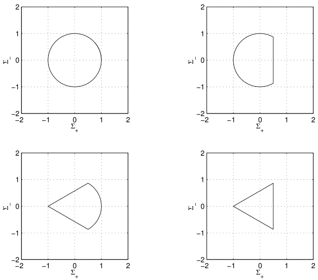
Figure 8. The points to which the shear variables may converge for a stiff fluid.

Proof. The theorem follows from Propositions 7.1 and 7.2. $\Box$

Consider now the case $2/3<\gamma<2$. Let $\mathcal{A}$ be the closure of the type II vacuum points.

Theorem 19.2.

Consider a generic Bianchi IX solution $x$ with $2/3<\gamma<2$. Then it converges to the closure of the set of vacuum type II points, that is

$$\lim_{\tau\rightarrow-\infty}\inf_{y\in\mathcal{A}}\|x(\tau)-y\|=0$$

where $\|\cdot\|$ is the Euclidean norm on $\mathbb{R}^{6}$. Furthermore, there are at least three non-special $\alpha$-limit points on the Kasner circle.

Remark. One can start out arbitrarily close to this set without converging to it, cf. Proposition 11.1.

Proof. The first part follows from Corollary 15.4 and the second part follows from Corollary 18.1. $\Box$

Proof of Theorems 1.1 and 1.2. Let $(M,g)$ be the Lorentz manifold obtained in Lemma 21.2 with topology $I\times G$. It is globally hyperbolic by Lemma 21.4.

If the initial data satisfy $\mathrm{tr}_{g}k=0$ for a development not of type IX, then it is causally geodesically complete and satisfies $\mu=0$ for the entire development, by Lemma 21.5 and Lemma 21.8. The first part of Theorem 1.1 follows.

Consider initial data of type I, II, V$\mathrm{I}_{0}$, VI$\mathrm{I}_{0}$ or VIII such that $\mathrm{tr}_{g}k\neq 0$. By Lemma 21.5 and Lemma 21.8, we may then time orient the development so that it is future causally geodesically complete and past causally geodesically incomplete, and the second part of Theorem 1.1 follows. The third part follows from Lemma 21.8.

Consider an inextendible future directed causal geodesic in the above development. Since each hypersurface $\{v\}\times G$ is a Cauchy hypersurface by Lemma 21.4, the causal curve exhausts the interval $I$.

1. If the solution is not of type IX, then the solution to (21.4)-(21.9), which is used in constructing the class A development, corresponds to a solution to (2.1)-(2.3), because of Lemma 21.5. Furthermore, $t\rightarrow t_{-}$ corresponds to $\tau\rightarrow-\infty$, because of Lemma 22.4.

a. In all the stiff fluid cases, the solution to (2.1)-(2.3) converges to a non-vacuum type I point by Theorem 19.1, so that Lemma 22.1 and Lemma 22.3 yield the desired conclusions in that case.

b. Type I, II and VI$\mathrm{I}_{0}$ with $1\leq\gamma<2$. That the Kretschmann scalar is unbounded in the cases stated in Theorem 1.2 follows from Proposition 8.1, Proposition 9.1, Proposition 10.2, Lemma 22.1 and and Lemma 22.2.

c. Non-vacuum solutions which are not of type IX. Then $\bar{R}_{\alpha\beta}\bar{R}^{\alpha\beta}$ is unbounded using Lemma 22.3.

2. If the solution is of type IX, then half of a solution to (21.4)-(21.9) corresponds to a Bianchi IX solution to (2.1)-(2.3), because of Lemma 21.6. By Lemma 22.5, $t\rightarrow t_{\pm}$ corresponds to $\tau\rightarrow-\infty$.

a. In the stiff fluid case, we get the desired statement as before.

b. If $1\leq\gamma<2$, we get the desired conclusions, concerning blow up of the Kretschmann scalar, from Corollary 18.1, Proposition 11.1, Lemma 22.1 and Lemma 22.2.

c. Non-vacuum solutions. Then $\bar{R}_{\alpha\beta}\bar{R}^{\alpha\beta}$ is unbounded using Lemma 22.3.

Let us now prove that the development is inextendible in the relevant cases. Assume there is a connected Lorentz manifold $(\hat{M},\hat{g})$ of the same dimension, and a map $i:M\rightarrow\hat{M}$ which is an isometry onto its image, with $i(M)\neq\hat{M}$. Then there is a $p\in\hat{M}-i(M)$ and a timelike geodesic $\gamma:[a,b]\rightarrow\hat{M}$ such that $\gamma([a,b))\subseteq i(M)$ and $\gamma(b)=p$. Since $\gamma|_{[a,b)}$ can be considered to be a future or past inextendible timelike geodesic in $M$, either it has infinite length or a curvature invariant blows up along it, by the above arguments. Both possibilities lead to a contradiction. Theorem 1.2 follows. $\Box$

20. Asymptotically velocity term dominated behaviour near the singularity

In this section, we consider the asymptotic behaviour of Bianchi VIII and IX stiff fluid solutions from another point of view. We wish to compare our results with [2], a paper which deals with analytic solutions of Einstein’s equations coupled to a scalar field or a stiff fluid. In [2], Andersson and Rendall prove that given a certain kind of solution to the so called velocity dominated system, there is a unique solution of Einstein’s equations coupled to a stiff fluid approaching the velocity dominated solution asymptotically. We will be more specific concerning the details below. The question which arises is to what extent it is natural to assume that a solution has the asymptotic behaviour they prescribe. We show here that all Bianchi VIII and IX stiff fluid solutions exhibit such asymptotic behaviour.

In order to speak about velocity term dominance, we need to have a foliation. In our case, there is a natural foliation given by the spatial hypersurfaces of homogeneity. Relative to this foliation, we can express the metric as in (21.14) according to Lemma 21.2. In what follows, we will use the frame $e_{i}^{\prime}$ appearing in Lemma 21.2, and Latin indices will refer to this frame. Let $g$ be the Riemannian metric, and $k$ the second fundamental form of the spatial hypersurfaces of homogeneity, so that

(20.1) $$g_{ij}=\bar{g}(e_{i}^{\prime},e_{j}^{\prime})=a_{i}^{-2}\delta_{ij},$$

where $\bar{g}$ is as in (21.14). The constraint equations in our situation are

(20.2) $$R-k_{ij}k^{ij}+(\mathrm{tr}k)^{2} = 2\mu$$

(20.3) $$\nabla^{i}k_{ij}-\nabla_{j}(\mathrm{tr}k) = 0,$$

which are the same as (21.8) and (21.5) respectively. The evolution equations are

(20.4) $$\partial_{t}g_{ij} = -2k_{ij}$$

(20.5) $$\partial_{t}k^{i}_{\ j} = R^{i}_{\ j}+(\mathrm{tr}k)k^{i}_{\ j}.$$

The evolution equation for the matter is

(20.6) $$\partial_{t}\mu=2(\mathrm{tr}k)\mu.$$

We wish to compare solutions to these equations with solutions to the so called velocity dominated system. This system also consists of constraints and evolution equations, and we will denote the velocity dominated solution with a left superscript zero. The constraints are

(20.7) $$-{}^{0}k_{ij}{}^{0}k^{ij}+(\mathrm{tr}{}^{0}k)^{2} = 2{}^{0}\mu$$

(20.8) $${}^{0}\nabla^{i}({}^{0}k_{ij})-{}^{0}\nabla_{j}(\mathrm{tr}{}^{0}k) = 0.$$

The evolution equations are

(20.9) $$\partial_{t}{}^{0}g_{ij} = -2{}^{0}k_{ij}$$

(20.10) $$\partial_{t}{}^{0}k^{i}_{\ j} = (\mathrm{tr}{}^{0}k){}^{0}k^{i}_{\ j},$$

and the matter equation is

(20.11) $$\partial_{t}{}^{0}\mu=2(\mathrm{tr}{}^{0}k){}^{0}\mu.$$

We raise and lower indices of the velocity dominated system with the velocity dominated metric. In [2], Andersson and Rendall prove that given an analytic solution to (20.7)-(20.11) on $S\times(0,\infty)$ such that $t\mathrm{tr}{}^{0}k=-1$, and such that the eigenvalues of $-t{}^{0}k^{i}_{\ j}$ are positive, there is a unique analytic solution to (20.2)-(20.6) asymptotic, in a suitable sense, to the solution of the velocity dominated system. In fact, they prove this statement in a more general setting than the one given above. We have specialized to our situation. Observe the condition on the eigenvalues of $-t{}^{0}k^{i}_{\ j}$. Our goal is to prove that this is a natural condition in the Bianchi VIII and IX cases.

Theorem 20.1.

Consider a Bianchi VIII or IX stiff fluid development as in Lemma 21.2 with $\mu_{0}>0$. Choose time coordinate so that $t_{-}=0$. Then there is a solution to (20.7)-(20.11) such that $t\mathrm{tr}{}^{0}k=-1$, the eigenvalues of $-t{}^{0}k^{i}_{\ j}$ are positive, and the following estimates hold

1. ${}^{0}g^{il}g_{lj}=\delta^{i}_{\ j}+o(t^{\alpha^{i}_{\ j}})$

2. $k^{i}_{\ j}={}^{0}k^{i}_{\ j}+o(t^{-1+\alpha^{i}_{\ j}})$

3. $\mu={}^{0}\mu+o(t^{-2+\beta_{1}})$,

where $\alpha^{i}_{\ j}$ and $\beta_{1}$ are positive real numbers.

Remark. In [2] two more estimates occur. They are not included here as they are replaced by equalities in our situation. Observe that the difficulties encountered in [2] concerning the non-diagonal terms of $k^{i}_{\ j}$ disappear in the present situation.

Proof. Below we will use the results of Lemma 21.2 and its proof implicitly. When we speak of $\theta_{ij}$, $\sigma_{ij}$, $\theta$, $n_{ij}$ and $\mu$, we will refer to the solution of (21.4)-(21.9) and the indices of these objects should not be understood in terms of evaluation on a frame. Since $\theta_{ij}$ and so on are all diagonal, we will sometimes write $\theta_{i}$ etc instead, denoting diagonal component $i$. There are two relevant frames: $e_{i}^{\prime}$ and $e_{i}=a_{i}e_{i}^{\prime}$. The latter frame yields $n_{ij}$ through (1.7). When we speak of $k^{i}_{\ j}$, $R_{ij}$ and so on, we will always refer to the frame $e_{i}^{\prime}$. We have

$$k^{i}_{\ j}=-\theta_{i}\delta^{i}_{\ j}$$

(no summation on $i$). The metric is given by (20.1) above. Let us choose

(20.12) $${}^{0}k^{i}_{\ j}=-{}^{0}\theta_{i}\delta^{i}_{\ j},$$

let ${}^{0}\theta={}^{0}\theta_{1}+{}^{0}\theta_{2}+{}^{0}\theta_{3}$ and

$${}^{0}g_{ij}={}^{0}a_{i}^{-2}\delta_{ij}$$

(no summation on $i$). Because of (20.12), equation (20.8) will be satisfied since it is a statement concerning the commutation of ${}^{0}k^{i}_{\ j}$ and $n_{ij}$. The existence interval for the solution to Einstein’s equations is $(0,t_{+})$ by our conventions, and since we wish to have $t\mathrm{tr}{}^{0}k=-1$ we need to define ${}^{0}\theta(t)=1/t$. Observe that ${}^{0}\theta_{i}/{}^{0}\theta$ is constant in time, and that $\theta_{i}/\theta$ converges to a positive value as $t\rightarrow 0$; this is a consequence of Theorem 19.1 and the definition (21.11) of the variables $\Sigma_{+}$ and $\Sigma_{-}$. Choose ${}^{0}\theta_{i}$ so that ${}^{0}\theta_{i}/{}^{0}\theta$ coincides with the limit of $\theta_{i}/\theta$. Similarly ${}^{0}\mu/{}^{0}\theta^{2}$ is constant, $\mu/\theta^{2}$ converges to a positive value, and we choose ${}^{0}\mu/{}^{0}\theta^{2}$ to be the limit. Since $R/\theta^{2}$ is a polynomial in the $N_{i}$ and the $N_{i}$ converge to zero by Theorem 19.1, equation (20.7) will be fulfilled. By our choices, (20.10) and (20.11) will also be fulfilled. We will specify the initial value of ${}^{0}a_{i}$ later on, and then define ${}^{0}a_{i}$ by demanding that (20.9) holds.

It will be of interest to estimate terms of the form $R^{i}_{\ j}/\theta^{2}$. These terms are quadratic polynomials in the $N_{i}$. By abuse of notation, we will write $N_{i}(\tau)$ when we wish to evaluate $N_{i}$ in the Wainwright-Hsu time (21.10) and $N_{i}(t)$ when we wish to evaluate in the time used in this theorem. By Theorem 19.1, there is an $\epsilon>0$ and a $\tau_{0}$ such that

$$|N_{i}(\tau)|\leq\exp(\epsilon\tau)$$

for all $\tau\leq\tau_{0}$. We wish to rewrite this estimate in terms of $t$. Let us begin with (21.12). Since we can assume that $q\leq 3$ for $\tau\leq\tau_{0}$ we get

$$\theta(\tau)\leq\exp[-4(\tau-\tau_{0})]\theta(\tau_{0}),$$

so that for $\tau_{1},\tau\leq\tau_{0}$ we get, using (21.10),

$$t(\tau)-t(\tau_{1})=\int_{\tau_{1}}^{\tau}\frac{3}{\theta}ds\geq\frac{3}{4\theta(\tau_{0})}(\exp[4(\tau-\tau_{0})]-\exp[4(\tau_{1}-\tau_{0})]).$$

Letting $\tau_{1}$ go to $-\infty$ and observing that $t(-\infty)=0$, cf. Lemma 22.4 and Lemma 22.5, we get for some constant $c$

$$e^{4\tau}\leq ct(\tau),$$

so that

$$N_{i}(t)\leq\exp(\epsilon\tau(t))\leq Ct^{\eta}$$

for some positive number $\eta$. Consequently expressions such as $R^{i}_{\ j}/\theta^{2}$ and $R/\theta^{2}$ satisfy similar bounds.

Let us now prove the estimates formulated in the statement of the theorem. Observe that for $t$ small enough, we have

$$-\theta=\mathrm{tr}k(t)=-(\int_{0}^{t}[\frac{R}{\theta^{2}}+1]ds)^{-1},$$

since the singularity is at $t=0$ and $\mathrm{tr}k$ must become unbounded at the singularity, cf. Lemma 22.4, 22.5 and (21.12). Thus we get

(20.13) $$\theta-{}^{0}\theta=-\int_{0}^{t}\frac{R}{\theta^{2}}ds\{t\int_{0}^{t}[\frac{R}{\theta^{2}}+1]ds\}^{-1}=o(t^{-1+\eta_{1}})$$

for some $\eta_{1}>0$. In order to make the estimates concerning $k^{i}_{\ j}$, we need only consider $\theta_{i}$ and ${}^{0}\theta_{i}$. We have

$$\partial_{t}(\frac{\theta_{i}}{\theta}-\frac{{}^{0}\theta_{i}}{{}^{0}\theta})=\partial_{t}\frac{\theta_{i}}{\theta}=\frac{\theta_{i}R-R^{i}_{\ i}\theta}{\theta^{2}}$$

with no summation on the $i$ in $R^{i}_{\ i}$. This computation, together with the estimates above and the fact that $\theta_{i}/\theta-{}^{0}\theta_{i}/{}^{0}\theta$ converges to zero, yields the estimate

(20.14) $$\frac{\theta_{i}}{\theta}-\frac{{}^{0}\theta_{i}}{{}^{0}\theta}=o(t^{\eta_{2}}),$$

for some $\eta_{2}>0$. However,

(20.15) $$\frac{\theta_{i}}{\theta}-\frac{{}^{0}\theta_{i}}{{}^{0}\theta}=\frac{\theta_{i}-{}^{0}\theta_{i}}{\theta}+\frac{{}^{0}\theta_{i}}{{}^{0}\theta}\frac{{}^{0}\theta-\theta}{\theta}.$$

Combining (20.13), (20.14) and (20.15), we get estimate $2$ of the theorem. Similarly, we have

$$\partial_{t}(\frac{\mu}{\theta^{2}}-\frac{{}^{0}\mu}{{}^{0}\theta^{2}})=\partial_{t}\frac{\mu}{\theta^{2}}=\frac{2\mu R}{\theta^{3}}.$$

Integrating, using the fact that $\mu/\theta^{2}$ converges to ${}^{0}\mu/{}^{0}\theta^{2}$, we get

(20.16) $$\frac{\mu}{\theta^{2}}-\frac{{}^{0}\mu}{{}^{0}\theta^{2}}=o(t^{\eta_{3}})$$

where $\eta_{3}>0$. Using

$$\frac{\mu}{\theta^{2}}-\frac{{}^{0}\mu}{{}^{0}\theta^{2}}=\frac{\mu-{}^{0}\mu}{\theta^{2}}+\frac{{}^{0}\mu}{{}^{0}\theta^{2}}\frac{{}^{0}\theta^{2}-\theta^{2}}{\theta^{2}},$$

(20.13) and (20.16), we get estimate $3$ of the theorem. Finally, we need to specify the initial value of ${}^{0}a_{i}$ and prove estimate $1$. Since

$$\partial_{t}a_{i}=-\theta_{i}a_{i},$$

(no summation on $i$) and similarly for ${}^{0}a_{i}$, we get

$$\partial_{t}\frac{a_{i}}{{}^{0}a_{i}}=\frac{a_{i}}{{}^{0}a_{i}}({}^{0}\theta_{i}-\theta_{i}).$$

By our estimates on ${}^{0}\theta_{i}-\theta_{i}$, we see that this implies that $a_{i}/{}^{0}a_{i}$ converges as $t\rightarrow 0$. Choose the value of ${}^{0}a_{i}$ at one point in time so that this limit is $1$. We thus get, using estimate $2$ of the theorem,

$$\frac{a_{i}}{{}^{0}a_{i}}-1=o(t^{\alpha^{i}_{\ j}}).$$

Estimate $1$ of the theorem now follows from this estimate and the fact that

$${}^{0}g^{il}g_{lj}=\left(\frac{{}^{0}a_{i}}{a_{i}}\right)^{2}\delta^{i}_{\ j}.$$

The theorem follows. $\Box$

21. Appendix

The goal of this appendix is to relate the asymptotic behaviour of solutions to the ODE (2.1)-(2.3) to the behaviour of the spacetime in the incomplete directions of inextendible causal curves. We proceed as follows.

1. First, we formulate Einstein’s equations as an ODE, assuming that the spacetime has a given structure (21.1). The first formulation is due to Ellis and MacCallum. We also relate this formulation to the one by Wainwight and Hsu.

2. Given initial data as in Definition 1.1, we then show how to construct a Lorentz manifold as in (21.1), satisfying Einstein’s equations and with initial data as specified, using the equations of Ellis and MacCallum. We also prove some properties of this development such as Global hyperbolicity and answer some questions concerning causal geodesic completeness.

3. Finally, we relate the asymptotic behaviour of solutions to (2.1)-(2.3) to the question of curvature blow up in the development obtained by the above procedure.

We consider a special class of spatially homogeneous four dimensional spacetimes of the form

(21.1) $$(\bar{M},\bar{g})=(I\times G,-dt^{2}+\chi_{ij}(t)\xi^{i}\otimes\xi^{j}),$$

where $I$ is an open interval, $G$ is a Lie group of class A, $\chi_{ij}$ is a smooth positive definite matrix and the $\xi^{i}$ are the duals of a left invariant basis on $G$. The stress energy tensor is assumed to be given by

(21.2) $$T=\mu dt^{2}+p(\bar{g}+dt^{2}),$$

where $p=(\gamma-1)\mu$. Below, Latin indices will be raised and lowered by $\delta_{ij}$.

Consider a four dimensional $(\bar{M},\bar{g})$ as in (21.1) with $G$ of class A. In order to define the different variables, we specify a suitable orthonormal basis. Let $e_{0}=\partial_{t}$ and $e_{i}=a_{i}^{\ j}Z_{j}$, i=1,2,3, be an orthonormal basis, where $a$ is a $C^{\infty}$ matrix valued function of $t$ and the $Z_{i}$ are the duals of $\xi^{i}$.

By the following argument, we can assume that $<\bar{\nabla}_{e_{0}}e_{i},e_{j}>=0$. Let the matrix valued function $A$ satisfy $e_{0}(A)+AB=0$, $A(0)=\mathrm{Id}$ where $B_{ij}=<\bar{\nabla}_{e_{0}}e_{i},e_{j}>$ and $\mathrm{Id}$ is the $3\times 3$ identity matrix. Then $A$ is smooth and $SO(3)$ valued and if $e_{i}^{\prime}=A_{i}^{\ j}e_{j}$, then $<\bar{\nabla}_{e_{0}}e_{i}^{\prime},e_{j}^{\prime}>=0$.

Let

(21.3) $$\theta(X,Y)=<\bar{\nabla}_{X}e_{0},Y>,$$

$\theta_{\alpha\beta}=\theta(e_{\alpha},e_{\beta})$ and $[e_{\beta},e_{\gamma}]=\gamma_{\beta\gamma}^{\alpha}e_{\alpha}$ where Greek indices run from $0$ to $3$. The objects $\theta_{\alpha\beta}$ and $\gamma_{\beta\gamma}^{\alpha}$ will be viewed as smooth functions from $I$ to some suitable $\mathbb{R}^{k}$, and our variables will be defined in terms of them.

Observe that $[Z_{i},e_{0}]=0$. The $e_{i}$ span the tangent space of $G$, and $<[e_{0},e_{i}],e_{0}>=0$. We get $\theta_{00}=\theta_{0i}=0$ and $\theta_{\alpha\beta}$ symmetric. We also have $\gamma_{ij}^{0}=\gamma_{0i}^{0}=0$ and $\gamma_{0j}^{i}=-\theta_{ij}$. We let $n$ be defined as in (1.7) and

$$\sigma_{ij}=\theta_{ij}-\frac{1}{3}\theta\delta_{ij},$$

where we by abuse of notation have written $\mathrm{tr}(\theta)$ as $\theta$.

We express Einstein’s equations in terms of $n$, $\sigma$ and $\theta$. The Jacobi identities for $e_{\alpha}$ yield

(21.4) $$e_{0}(n_{ij})-2n_{k(i}\sigma_{j)}^{\ k}+\frac{1}{3}\theta n_{ij}=0.$$

The $0i$-components of the Einstein equations are equivalent to

(21.5) $$\sigma_{i}^{\ k}n_{kj}-n_{i}^{\ k}\sigma_{kj}=0.$$

Letting $b_{ij}=2n_{i}^{\ k}n_{kj}-\mathrm{tr}(n)n_{ij}$ and $s_{ij}=b_{ij}-\frac{1}{3}\mathrm{tr}(b)\delta_{ij}$, the trace free part of the $ij$ equations are

(21.6) $$e_{0}(\sigma_{ij})+\theta\sigma_{ij}+s_{ij}=0.$$

The $00$-component yields the Raychaudhuri equation

(21.7) $$e_{0}(\theta)+\theta_{ij}\theta^{ij}+\frac{1}{2}(3\gamma-2)\mu=0,$$

and using this together with the trace of the $ij$-equations yields a constraint

(21.8) $$\sigma_{ij}\sigma^{ij}+(n_{ij}n^{ij}-\frac{1}{2}\mathrm{tr}(n)^{2})+2\mu=\frac{2}{3}\theta^{2}.$$

Equations (21.4)-(21.8) are special cases of equations given in Ellis and MacCallum [8]. At a point $t_{0}$, we may diagonalize $n$ and $\sigma$ simultaneously since they commute (21.5). Rotating $e_{\alpha}$ by the corresponding element of $SO(3)$ yields upon going through the definitions that the new $n$ and $\sigma$ are diagonal at $t_{0}$. Collect the off-diagonal terms of $n$ and $\sigma$ in one vector $v$. By (21.4) and (21.6), there is a time dependent matrix $C$ such that $\dot{v}=Cv$ so that $v(t)=0$ for all $t$, since $v(t_{0})=0$. Since the rotation was time independent, $<\nabla_{e_{0}}e_{i},e_{j}>=0$ holds in the new basis.

The fact that $T$ is divergence free yields

(21.9) $$e_{0}(\mu)+\gamma\theta\mu=0.$$

Introduce, as in Wainwright and Hsu [17],

$$\Sigma_{ij}=\sigma_{ij}/\theta$$

$$N_{ij}=n_{ij}/\theta$$

$$\Omega=3\mu/\theta^{2}$$

and define a new time coordinate $\tau$, independent of time orientation, satisfying

(21.10) $$\frac{dt}{d\tau}=\frac{3}{\theta}.$$

For Bianchi IX developments, we only consider the part of spacetime where $\theta$ is strictly positive or strictly negative. Let

(21.11) $$\Sigma_{+}=\frac{3}{2}(\Sigma_{22}+\Sigma_{33})\ \mathrm{and}\ \Sigma_{-}=\frac{\sqrt{3}}{2}(\Sigma_{22}-\Sigma_{33}).$$

If we let $N_{i}$ be the diagonal elements of $N_{ij}$, equations (21.4) and (21.6) turn into (2.1) with definitions as in (2.2), except for the expression for $\Omega^{\prime}$. It can however be derived from (21.9). The constraint (21.8) turns into (2.3). The Raychaudhuri equation (21.7) takes the form

(21.12) $$\theta^{\prime}=-(1+q)\theta.$$

Before using the equations of Ellis and MacCallum to construct a development, it is convenient to know that one can make some simplifying assumptions concerning the choice of basis. The next lemma fulfills this objective, and also proves the classification of the class A Lie algebras mentioned in the introduction.

Lemma 21.1.

Table 1 constitutes a classification of the class A Lie algebras. Consider an arbitrary basis $\{e_{i}\}$ of the Lie algebra. Then by applying an orthogonal matrix to it, we can construct a basis $\{e_{i}^{\prime}\}$ such that the corresponding $n^{\prime}$ defined by (1.7) is diagonal, with diagonal elements of one of the types given in Table 1.

Proof. Let $e_{i}$ be a basis for the Lie algebra and $n$ be defined as in (1.7). If we change the basis according to $e_{i}^{\prime}=(A^{-1})_{i}^{\ j}e_{j}$, then $n$ transforms to

(21.13) $$n^{\prime}=(\det A)^{-1}A^{t}nA$$

Since $n$ is symmetric, we assume from here on that the basis is such that it is diagonal. The matrix $A=\mathrm{diag}(1\ 1\ -1)$ changes the sign of $n$. A suitable orthogonal matrix performs even permutations of the diagonal. The number of non-zero elements on the diagonal is invariant under transformations (21.13) taking one diagonal matrix to another. If $A=(a_{ij})$ and the diagonal matrix $n^{\prime}$ is constructed as in (21.13), we have $n^{\prime}_{kk}=(\det A)^{-1}\sum_{i=1}^{3}a_{ik}^{2}n_{ii}$, so that if all the diagonal elements of $n$ have the same sign, the same is true for $n^{\prime}$. The statements of the lemma follow. $\Box$

We now prove that if we begin with initial data as in Definition 1.1, we get a development as in Definition 1.4 of the form (21.1), with certain properties.

Lemma 21.2.

Fix $2/3<\gamma\leq 2$. Let $G,\ g,\ k$ and $\mu_{0}$ be initial data as in Definition 1.1. Then there is an orthonormal basis $e_{i}^{\prime}$ $i=1,2,3$ of the Lie algebra such that $n_{ij}^{\prime}$ defined by (1.7) and $k_{ij}=k(e_{i}^{\prime},e_{j}^{\prime})$ are diagonal and $n_{ij}^{\prime}$ is of one of the forms given in Table 1. Let

$$\theta(0)=-\mathrm{tr}_{g}k,\ \sigma_{ij}(0)=-k(e_{i}^{\prime},e_{j}^{\prime})+\frac{1}{3}\theta(0)\delta_{ij},\ n_{ij}(0)=n_{ij}^{\prime}\ and\ \mu(0)=\mu_{0}.$$

Solve (21.4), (21.6), (21.7) and (21.9) with these conditions as initial data to obtain $n,\ \sigma,\ \theta$ and $\mu$, and let $I$ be the corresponding existence interval. Then there are smooth functions $a_{i}:I\rightarrow(0,\infty)$ $i=1,2,3$, with $a_{i}(0)=1$, such that

(21.14) $$\bar{g}=-dt^{2}+\sum_{i=1}^{3}a_{i}^{-2}(t)\xi^{i}\otimes\xi^{i},$$

where $\xi^{i}$ is the dual of $e_{i}^{\prime}$, satisfies Einstein’s equations (1.3) on $\bar{M}=I\times G$, with $T$ as in (1.1) with $u=e_{0}$, $\mu$ as above and $p=(\gamma-1)\mu$. Furthermore,

$$<\bar{\nabla}_{e_{i}}e_{0},e_{j}>=\sigma_{ij}+\frac{1}{3}\theta\delta_{ij},$$

where $\bar{\nabla}$ is the Levi-Civita connection of $\bar{g}$ and $e_{i}=a_{i}e_{i}^{\prime}$, if we consider the left hand side to be a function of $t$. Consequently, the induced metric and second fundamental form on $\{0\}\times G$ are $g$ and $k$, and we have a development satisfying the conditions of Definition 1.4.

Proof. Let $e_{i}^{\prime}$, $i=1,2,3$ be a left invariant orthonormal basis. We can assume the corresponding $n^{\prime}$ to be of one of the forms given in Table 1 by Lemma 21.1. The content of (1.5) is that $k_{ij}=k(e_{i}^{\prime},e_{j}^{\prime})$ and $n^{\prime}$ are to commute. We may thus also assume $k_{ij}$ to be diagonal without changing the earlier conditions of the construction. If we let $n(0)=n^{\prime}$, $\theta(0)=-\mathrm{tr}_{g}k$, $\sigma_{ij}(0)=-k_{ij}+\theta\delta_{ij}/3$ and $\mu(0)=\mu_{0}$, then (1.4) is the same as (21.8). Let $n$, $\sigma$, $\theta$ and $\mu$ satisfy (21.4), (21.6), (21.7) and (21.9) with initial values as specified above. Since (21.8) is satisfied at $0$, it is satisfied for all times. For reasons given in connection with (21.8), $n$ and $\sigma$ will remain diagonal so that (21.5) will always hold. Let $n_{i}$ and $\sigma_{i}$ denote the diagonal elements of $n$ and $\sigma$ respectively.

How are we to define the $a_{i}$ in the statement of the lemma? The $\tilde{n}$ obtained from $e_{i}$ by (1.7) should coincide with $n$. This leads us to the following definitions. Let $f_{i}(0)=1$ and $\dot{f_{i}}/f_{i}=2\sigma_{i}-\theta/3$. Let $a_{i}=(\Pi_{j\neq i}f_{j})^{1/2}$ and define $e_{i}=a_{i}e_{i}^{\prime}$. Then $\tilde{n}$ associated to $e_{i}$ equals $n$. We complete the basis by letting $e_{0}=\partial_{t}$. Define a metric $<\cdot,\cdot>$ on $\bar{M}$ by demanding $e_{\alpha}$ to be orthonormal with $e_{0}$ timelike and $e_{i}$ spacelike, and let $\bar{\nabla}$ be the associated Levi-Civita connection. Compute $<\bar{\nabla}_{e_{0}}e_{i},e_{j}>=0$. If $\tilde{\theta}(X,Y)=<\bar{\nabla}_{X}e_{0},Y>$ and $\tilde{\theta}_{\mu\nu}=\tilde{\theta}(e_{\mu},e_{\nu})$, then $\tilde{\theta}_{00}=\tilde{\theta}_{i0}=\tilde{\theta}_{0i}=0$. Furthermore,

$$\frac{1}{a_{j}}e_{0}(a_{j})\delta_{ij}=-\tilde{\theta}_{ij}$$

(no summation over $j$) so that $\tilde{\theta}_{ij}$ is diagonal and $\mathrm{tr}\tilde{\theta}=\theta$. Finally,

$$-\tilde{\sigma}_{ii}=-\tilde{\theta}_{ii}+\frac{1}{3}\theta=-\sigma_{i}.$$

The lemma follows by considering the derivation of the equations of Ellis and MacCallum. $\Box$

Definition 21.1.

A development as in Lemma 21.2 will be called a class A development. We will also assign a type to such a development according to the type of the initial data.

The next thing to prove is that each $\bar{M}_{v}=\{v\}\times G$ is a Cauchy surface, but first we need a lemma.

Lemma 21.3.

Let $\rho$ be a left invariant Riemannian metric on a Lie group $G$. Then $\rho$ is geodesically complete.

Proof. Assume $\gamma:(t_{-},t_{+})\rightarrow G$ is a geodesic satisfying $\rho(\gamma^{\prime},\gamma^{\prime})=1$, with $t_{+}<\infty$. There is a $\delta>0$ such that every geodesic $\lambda$ satisfying $\lambda(0)=e$, the identity element of $G$, and $\lambda^{\prime}(0)=v$ with $\rho(v,v)\leq 1$ is defined on $(-\delta,\delta)$. If $L_{h}:G\rightarrow G$ is defined by $L_{h}(h_{1})=hh_{1}$, then $L_{h}$ is by definition an isometry. Let $t_{0}\in(t_{-},t_{+})$ satisfy $t_{+}-t_{0}\leq\delta/2$. Let $v\in T_{e}G$ be the vector corresponding to $\gamma^{\prime}(t_{0})$ under the isometry $L_{\gamma(t_{0})}$. Let $\lambda$ be a geodesic with $\lambda(0)=e$ and $\lambda^{\prime}(0)=v$. Then $L_{\gamma(t_{0})}\circ\lambda$ is a geodesic extending $\gamma$. $\Box$

Let us be precise concerning the concept Cauchy surface.

Definition 21.2.

Consider a time oriented Lorentz manifold $(M,g)$. Let $I$ be an interval in $\mathbb{R}$ and $\gamma:I\rightarrow M$ be a continuous map which is smooth except for a finite number of points. We say that $\gamma$ is a future directed causal, timelike or null curve if at each $t\in I$ where $\gamma$ is differentiable, $\gamma^{\prime}(t)$ is a future oriented causal, timelike or null vector respectively. We define past directed curves similarly. A causal curve is a curve which is either a future directed causal curve or a past directed causal curve and similarly for timelike and null curves. If there is a curve $\lambda:I_{1}\rightarrow M$ such that $\gamma(I)$ is properly contained in $\lambda(I_{1})$, then $\gamma$ is said to be extendible, otherwise it is called inextendible. A subset $S\subset M$ is called a Cauchy surface if it is intersected exactly once by every inextendible causal curve. A Lorentz manifold as above which admits a Cauchy surface is said to be Globally hyperbolic.

Lemma 21.4.

For a class A development, each $\bar{M}_{v}=\{v\}\times G$ is a Cauchy surface.

Proof. The metric is given by (21.14). A causal curve cannot intersect $\bar{M}_{v}$ twice since the $t$-component of such a curve must be strictly monotone. Assume that $\gamma:(s_{-},s_{+})\rightarrow M$ is an inextendible causal curve that never intersects $\bar{M}_{v}$. Let $\tilde{t}:\bar{M}\rightarrow I$ be defined by $\tilde{t}[(s,h)]=s$. Let $s_{0}\in(s_{-},s_{+})$ and assume that $\tilde{t}(\gamma(s_{0}))=t_{1}<v$ and that $<\gamma^{\prime},\partial_{t}><0$ where it is defined. Thus $\tilde{t}(\gamma(s))$ increases with $s$ and $\tilde{t}(\gamma([s_{0},s_{+})))\subseteq[t_{1},v]$. Since we have uniform bounds on $a_{i}$ from below and above on $[t_{1},v]$ and the curve is causal, we get

(21.15) $$(\sum_{i=1}^{3}\xi^{i}(\gamma^{\prime})^{2})^{1/2}\leq-C<\gamma^{\prime},e_{0}>$$

on that interval, with $C>0$. Since

(21.16) $$\int_{s_{0}}^{s_{+}}-<\gamma^{\prime},e_{0}>ds=\int_{s_{0}}^{s_{+}}\frac{d\tilde{t}\circ\gamma}{ds}ds\leq v-t_{1},$$

the curve $\gamma|_{[s_{0},s_{+})}$, projected to $G$, will have finite length in the metric $\rho$ on $G$ defined by making $e_{i}^{\prime}$ an orthonormal basis. Since $\rho$ is a left invariant metric on a Lie group, it is complete by Lemma 21.3, and sets closed and bounded in the corresponding topological metric must be compact. Adding the above observations, we conclude that $\gamma([s_{0},s_{+}))$ is contained in a compact set, and thus there is a sequence $s_{k}\in[s_{0},s_{+})$ with $s_{k}\rightarrow s_{+}$ such that $\gamma(s_{k})$ converges. Since $\tilde{t}(\gamma(s))$ is monotone and bounded it converges. Using (21.15) and an analogue of (21.16), we conclude that $\gamma$ has to converge as $s\rightarrow s_{+}$. Consequently, $\gamma$ is extendible contradicting our assumption. By this and similar arguments covering the other cases, we conclude that $\bar{M}_{v}$ is a Cauchy surface for each $v\in(t_{-},t_{+})$. $\Box$

Before we turn to the questions concerning causal geodesic completeness, let us consider the evolution of $\theta$ for solutions to the equations of Ellis and MacCallum. This is relevant also for the definition of the variables of Wainwright and Hsu, since there one divides by $\theta$. We first consider developments as in Lemma 21.2 which are not of type IX.

Lemma 21.5.

Consider class A developments which are not of type IX. Let the existence interval be $I=(t_{-},t_{+})$. Then there are two possibilities.

1. $\theta\neq 0$ for the entire development. We then time orient the manifold so that $\theta>0$. With this time orientation, $t_{+}=\infty$.

2. $\theta=0$, $\sigma_{ij}=0$ and $\mu=0$ for the entire development. Furthermore, $n_{ij}$ is constant and diagonal and two of the diagonal components are equal and the third is zero. The only Bianchi types which admit this possibility are thus type I and type VI$I_{0}$. Furthermore $I=(-\infty,\infty)$.

Proof. Since $n_{ij}$ is diagonal, see the proof of Lemma 21.2, we can formulate the constraint (21.8) as

$$\sigma_{ij}\sigma^{ij}+\frac{1}{2}[n_{1}^{2}+(n_{2}-n_{3})^{2}-2n_{1}(n_{2}+n_{3})]+2\mu=\frac{2}{3}\theta^{2},$$

where the $n_{i}$ are the diagonal components of $n_{ij}$. Considering Table 1, we see that, excepting type IX, the expression in the $n_{i}$ is always non-negative. Thus we deduce the inequality

(21.17) $$\sigma_{ij}\sigma^{ij}+2\mu\leq\frac{2}{3}\theta^{2}.$$

Combining it with (21.7), we get $|e_{0}(\theta)|\leq\theta^{2}$, using the fact that $2/3<\gamma\leq 2$. Consequently, if $\theta$ is zero once, it is always zero. Time orient the developments with $\theta\neq 0$ so that $\theta>0$.

Consider the possibility $\theta=0$. Equation (21.7) then implies $\sigma_{ij}=0$ and $\mu=0$, since $\gamma>2/3$. Equations (21.8) and (21.6) then imply $b_{ij}=0$, and (21.4) implies $n_{ij}$ constant. All the statements except the the fact that $t_{+}=\infty$ in the $\theta>0$ case follow from the above.

Observe that $\theta$ decreases in magnitude with time, so that it is bounded to the future. By the (21.17), the same is true of $\sigma_{ij}$ and $\mu$. Using (21.4), we get control of $n_{ij}$ and conclude that the solution may not blow up in finite time. We must thus have $t_{+}=\infty$. $\Box$

By a theorem of Lin and Wald [14], Bianchi IX developments recollapse.

Lemma 21.6.

Consider a Bianchi IX class A development with $1\leq\gamma\leq 2$ and $I=(t_{-},t_{+})$. Then there is a $t_{0}\in I$ such that $\theta>0$ in $(t_{-},t_{0})$ and $\theta<0$ in $(t_{0},t_{+})$.

Proof. Let us begin by proving that $\theta$ can be zero at most once. If $\theta(t_{i})=0$, $i=1,2$ and $t_{1}<t_{2}$, then $\theta=0$ in $(t_{1},t_{2})$ since it is monotone by (21.7). Thus (21.7) implies $\sigma_{ij}=0=\mu$ in $(t_{1},t_{2})$ as well. Combining this fact with (21.8) and (21.6), we get $b_{ij}=0$, which is impossible for a Bianchi IX solution. Assume $\theta$ is never zero. By a suitable choice of time orientation, we can assume that $\theta>0$ on $I$. Let us prove that $t_{+}=\infty$. Since $\theta$ is decreasing on $I_{1}=[0,t_{+})$ and non-negative on $I$ it is bounded on $I_{1}$. By (21.4), $n_{1}n_{2}n_{3}$ decreases so that it is bounded on $I_{1}$. By an argument similar to the proof of Lemma 3.3, one can combine this bound with (21.8) to conclude that $\sigma_{ij}$ and $\mu$ are bounded on $I_{1}$. By (21.4), we conclude that $n_{ij}$ cannot grow faster than exponentially. Consequently, the future existence interval must be infinite, that is $t_{+}=\infty$, since $I$ was the maximal existence interval and solutions cannot blow up in finite time. In order to use the arguments of Lin and Wald, we define

$$\beta_{i}(t)=\int_{0}^{t}\sigma_{i}(s)ds+\beta_{i}^{0},\ \alpha(t)=\int_{0}^{t}\frac{1}{3}\theta(s)ds+\alpha_{0},$$

where $2\beta_{i}^{0}-\alpha_{0}=\ln(n_{i}(0))$ and $\sum_{i=1}^{3}\beta_{i}^{0}=0$. Then

$$n_{i}=\exp(2\beta_{i}-\alpha).$$

Let $\rho=\mu/8\pi$ and $P_{i}=p/8\pi=(\gamma-1)\mu/8\pi$, $i=1,2,3$. Equations (21.8) and (21.7) then imply equations (1.4) and (1.5) of [14], and equations (1.6) and (1.7) of [14] follow from (21.6). We have thus constructed a solution to (1.4)-(1.7) of [14] on an interval $[0,\infty)$ with $d\alpha/dt>0$. Lin and Wald prove in their paper [14] that this assumption leads to a contradiction, if one assumes that $|P_{i}|\leq\rho$ and $P_{1}+P_{2}+P_{3}\geq 0$. However, these conditions are fulfilled in our situation, assuming $1\leq\gamma\leq 2$. In other words, there is a zero and since $\theta$ is decreasing it must be positive before the zero and negative after it. The lemma follows. $\Box$

The lemma concerning causal geodesic completeness will build on the following estimate.

Lemma 21.7.

Consider a class A development. Let $\gamma:(s_{-},s_{+})\rightarrow\bar{M}$ be a future directed inextendible causal geodesic, and

(21.18) $$f_{\nu}(s)=<\gamma^{\prime}(s),e_{\nu}|_{\gamma(s)}>.$$

If $\theta=0$ for the entire development, then $f_{0}$ is constant. Otherwise,

(21.19) $$\frac{d}{ds}(f_{0}\theta)\geq\frac{2-\sqrt{2}}{3}\theta^{2}f_{0}^{2}.$$

Remark. We consider functions of $t$ as functions of $s$ by evaluating them at $\tilde{t}(\gamma(s))$, where $\tilde{t}$ is the function defined in Lemma 21.4.

Proof. Compute, using the proof of Lemma 21.2,

$$\frac{df_{0}}{ds}=<\gamma^{\prime}(s),\nabla_{\gamma^{\prime}(s)}e_{0}>=\sum_{k=1}^{3}\theta_{k}f_{k}^{2},$$

where $\theta_{k}$ are the diagonal elements of $\theta_{ij}$. If $\theta=0$ for the entire development, then $\theta_{k}=0$ for the entire development by Lemma 21.5 and Lemma 21.6, so that $f_{0}$ is constant. Compute, using Raychaudhuri’s equation (21.7),

$$\frac{d}{ds}(f_{0}\theta)=\frac{1}{3}\theta^{2}\sum_{k=1}^{3}f_{k}^{2}+\sum_{k=1}^{3}\theta\sigma_{k}f_{k}^{2}+f_{0}^{2}\sum_{k=1}^{3}\sigma_{k}^{2}+\frac{1}{3}\theta^{2}f_{0}^{2}+\frac{1}{2}(3\gamma-2)\mu f_{0}^{2}$$

where $\sigma_{k}$ are the diagonal elements of $\sigma_{ij}$. Estimate

$$|\sum_{k=1}^{3}\sigma_{k}f_{k}^{2}|\leq\left(\frac{2}{3}\right)^{1/2}\left(\sum_{k=1}^{3}\sigma_{k}^{2}\right)^{1/2}\sum_{k=1}^{3}f_{k}^{2},$$

using the tracelessness of $\sigma_{ij}$. By making a division into the three cases $\sum_{k=1}^{3}\sigma_{k}^{2}\leq\theta^{2}/3$, $\theta^{2}/3\leq\sum_{k=1}^{3}\sigma_{k}^{2}\leq 2\theta^{2}/3$ and $2\theta^{2}/3\leq\sum_{k=1}^{3}\sigma_{k}^{2}$, and using the causality of $\gamma$ we deduce (21.19). $\Box$

Lemma 21.8.

Consider a class A development with existence interval $I=(t_{-},t_{+})$. There are three possibilities.

1. $\theta=0$ for the entire development, in which case the development is causally geodesically complete.

2. The development is not of type IX and $\theta>0$. Then all inextendible causal geodesics are future complete and past incomplete. Furthermore, $t_{-}>-\infty$ and $t_{+}=\infty$.

3. If the development is of type IX with $1\leq\gamma\leq 2$, then all inextendible causal geodesics are past and future incomplete. We also have $t_{-}>-\infty$ and $t_{+}<\infty$.

Proof. Let $\gamma:(s_{-},s_{+})\rightarrow\bar{M}$ be a future directed inextendible causal geodesic and $f_{\nu}$ be defined as in (21.18). Let furthermore $I=(t_{-},t_{+})$ be the existence interval mentioned in Lemma 21.2. Since every $\bar{M}_{v}$, $v\in I$ is a Cauchy surface by Lemma 21.4, $\tilde{t}(\gamma(s))$ must cover the interval $I$ as $s$ runs through $(s_{-},s_{+})$. Furthermore, $\tilde{t}(\gamma(s))$ is monotone increasing so that

(21.20) $$\tilde{t}(\gamma(s))\rightarrow t_{\pm}\ \mathrm{as}\ s\rightarrow s_{\pm}.$$

Let $s_{0}\in(s_{-},s_{+})$ and compute

(21.21) $$\int_{s_{0}}^{s}-f_{0}(u)du=\tilde{t}(\gamma(s))-\tilde{t}(\gamma(s_{0})).$$

Consider the case $\theta=0$ for the entire development. By Lemma 21.7, $f_{0}$ is then constant, and $I=(-\infty,\infty)$ by Lemma 21.5. Equations (21.21) and (21.20) then prove that we must have $(s_{-},s_{+})=(-\infty,\infty)$. Thus, all inextendible causal geodesics must be complete.

Assume that the development is not of type IX and that $\theta>0$. Since $f_{0}\theta$ is negative on $[s_{0},s_{+})$, its absolute value is bounded on that interval by (21.19). If $s_{+}$ were finite, $\theta$ would be bounded from below by a positive constant on $[s_{0},s_{+})$, since

$$|\frac{d\theta}{ds}|\leq-f_{0}\theta^{2}\leq C\theta$$

on that interval for some $C>0$, cf. (21.17) and the observations following that equation. Since $f_{0}\theta$ is bounded, we then deduce that $f_{0}$ is bounded on $[s_{0},s_{+})$. But then (21.20) and (21.21) cannot both hold, since $t_{+}=\infty$ by Lemma 21.5. Thus, $s_{+}=\infty$ and all inextendible causal geodesics must future complete. Since $f_{0}\theta$ is negative on $(s_{-},s_{+})$, (21.19) proves that this expression must blow up in finite $s$-time going backward, so that $s_{-}>-\infty$. Since the curve $\gamma(s)=(s,e)$ is an inextendible timelike geodesic, we conclude that $t_{-}>-\infty$.

Consider the Bianchi IX case. By Lemma 21.4 and 21.6, we conclude the existence of an $s_{0}\in(s_{-},s_{+})$ such that $f_{0}\theta$ is negative on $(s_{-},s_{0})$ and positive on $(s_{0},s_{+})$. By (21.19), $f_{0}\theta$ must blow up a finite $s$-time before $s_{0}$, and a finite $s$-time after $s_{0}$. Every inextendible causal geodesic is thus future and past incomplete. We conclude $t_{-}>-\infty$ and $t_{+}<\infty$. $\Box$

22. Appendix

In this appendix, we consider the curvature expressions. According to [19], p. 40, the Weyl tensor $\bar{C}_{\alpha\beta\gamma\delta}$ is defined by

$$\bar{R}_{\alpha\beta\gamma\delta}=\bar{C}_{\alpha\beta\gamma\delta}+(\bar{g}_{\alpha[\gamma}\bar{R}_{\delta]\beta}-\bar{g}_{\beta[\gamma}\bar{R}_{\delta]\alpha})-\frac{1}{3}\bar{R}\bar{g}_{\alpha[\gamma}\bar{g}_{\delta]\beta},$$

where the bar in $\bar{g}_{\alpha\beta}$ and so on indicates that we are dealing with spacetime objects as opposed to objects on a spatial hypersurface. Using this relation and the fact that our spacetime satisfies (1.3), where $T$ is given by (1.1) and (1.2), one can derive the following expression for the Kretschmann scalar

(22.1) $$\kappa=\bar{R}_{\alpha\beta\gamma\delta}\bar{R}^{\alpha\beta\gamma\delta}=\bar{C}_{\alpha\beta\gamma\delta}\bar{C}^{\alpha\beta\gamma\delta}+2\bar{R}_{\alpha\beta}\bar{R}^{\alpha\beta}-\frac{1}{3}\bar{R}^{2}=$$

$$=\bar{C}_{\alpha\beta\gamma\delta}\bar{C}^{\alpha\beta\gamma\delta}+\frac{1}{3}[4+(3\gamma-2)^{2}]\mu^{2}.$$

However, according to [18], p. 19, we have

(22.2) $$\bar{C}_{\alpha\beta\gamma\delta}\bar{C}^{\alpha\beta\gamma\delta}=8(E_{\alpha\beta}E^{\alpha\beta}-H_{\alpha\beta}H^{\alpha\beta}),$$

where, relative to the frame $e_{\alpha}$ appearing in Lemma 21.2, all components of $E$ and $H$ involving $e_{0}$ are zero, and the $ij$ components are given by

$$E_{ij} = \frac{1}{3}\theta\sigma_{ij}-(\sigma_{i}^{\ k}\sigma_{kj}-\frac{1}{3}\sigma_{kl}\sigma^{kl}\delta_{ij})+s_{ij}$$

$$H_{ij} = -3\sigma^{k}_{\ (i}n_{j)k}+n_{kl}\sigma^{kl}\delta_{ij}+\frac{1}{2}n^{k}_{\ k}\sigma_{ij},$$

where $s_{ij}$ is the same expression that appears in (21.6), see p. 40 of [18]. Observe that in our situation, $E$ and $H$ are diagonal, since we are interested in the developments obtained in Lemma 21.2. It is natural to normalize $\tilde{E}_{ij}=E_{ij}/\theta^{2}$ and similarly for $H$. We will denote the diagonal components of $\tilde{E}_{ij}$ by $\tilde{E}_{i}$. We want to have expressions in $\Sigma_{+}$, $\Sigma_{-}$ and so on, and therefore we compute

$$\tilde{H}_{1} = N_{1}\Sigma_{+}+\frac{1}{\sqrt{3}}(N_{2}-N_{3})\Sigma_{-}$$

$$\tilde{H}_{2} = -\frac{1}{2}N_{2}(\Sigma_{+}+\sqrt{3}\Sigma_{-})+\frac{1}{2}(N_{3}-N_{1})(\Sigma_{+}-\frac{1}{\sqrt{3}}\Sigma_{-})$$

$$\tilde{E}_{2}-\tilde{E}_{3} = \frac{2}{3\sqrt{3}}\Sigma_{-}(1-2\Sigma_{+})+(N_{2}-N_{3})(N_{2}+N_{3}-N_{1})$$

$$\tilde{E}_{2}+\tilde{E}_{3} = \frac{2}{9}\Sigma_{+}(1+\Sigma_{+})-\frac{2}{9}\Sigma_{-}^{2}-\frac{2}{3}N_{1}^{2}+\frac{1}{3}(N_{2}-N_{3})^{2}+\frac{1}{3}N_{1}(N_{2}+N_{3}).$$

Observe that all other components of $\tilde{E}_{i}$ and $\tilde{H}_{i}$ can be computed from this, as $E_{ij}$ and $H_{ij}$ are both traceless.

It is convenient to define the normalized Kretschmann scalar

(22.3) $$\tilde{\kappa}=R_{\alpha\beta\gamma\delta}R^{\alpha\beta\gamma\delta}/\theta^{4}.$$

The latter object can be expressed as a polynomial in the variables of Wainwright and Hsu. By the above observations and the fact that $\Omega=3\mu/\theta^{2}$, we have

$$\tilde{\kappa}=8[\frac{3}{2}(\tilde{E}_{2}+\tilde{E}_{3})^{2}+\frac{1}{2}(\tilde{E}_{2}-\tilde{E}_{3})^{2}-2\tilde{H}_{1}^{2}-2\tilde{H}_{2}^{2}-2\tilde{H}_{1}\tilde{H}_{2}]+\frac{1}{27}[4+(3\gamma-2)^{2}]\Omega^{2}.$$

We will associate a $\kappa$ and a $\bar{R}_{\alpha\beta}\bar{R}^{\alpha\beta}$ to a solution to (2.1)-(2.3) in the following way. Since $\kappa/\theta^{4}$ can be expressed in terms of the variables of Wainwright and Hsu, it is natural to define $\kappa$ by this expression multiplied by $\theta^{4}$, where $\theta$ obeys (21.12). There is of course an ambiguity as to the initial value of $\theta$, but we are only interested in the asymptotics, and any non-zero value will yield the same conclusion. We associate $\bar{R}_{\alpha\beta}\bar{R}^{\alpha\beta}$ to a solution similarly.

Lemma 22.1.

The normalized Kretschmann scalar (22.3) is non-zero at the fixed points $F,\ P_{i}^{+}(II)$, at the non-special points on the Kasner circle, and at the type I stiff fluid points with $\Omega>0$. Consequently

(22.4) $$\limsup_{\tau\rightarrow-\infty}|\kappa(\tau)|=\infty$$

for all solutions to (2.1)-(2.3) which have one such point as an $\alpha$-limit point.

Proof. The statement concerning the normalized Kretschmann scalar is a computation. Equation (22.4) is a consequence of this computation, the fact that $\kappa=\tilde{\kappa}\theta^{4}$ and the fact that $\theta\rightarrow\infty$ as $\tau\rightarrow-\infty$, cf. (21.12). $\Box$

For some non-vacuum Taub type solutions with $2/3<\gamma<2$, the following lemma is needed.

Lemma 22.2.

Consider a solution to (2.1)-(2.3) with $\Omega>0$ and $2/3<\gamma<2$ such that

(22.5) $$\lim_{\tau\rightarrow-\infty}(\Sigma_{+},\Sigma_{-})=(-1,0).$$

Then

$$\lim_{\tau\rightarrow-\infty}\kappa(\tau)=\infty.$$

Proof. By Proposition 3.1, the solution must satisfy $\Sigma_{-}=0$ and $N_{2}=N_{3}$. Observe that because of (22.5), we have $\Omega\rightarrow 0$, since $\Omega$ decays exponentially for $\Sigma_{+}^{2}$ large, cf. the proof of Lemma 14.1. Consequently, $q\rightarrow 2$. One can then prove that for any $\epsilon>0$, there is a $T$ such that

(22.6) $$\exp[(a_{\gamma}+\epsilon)\tau]\leq\Omega(\tau)\leq\exp[(a_{\gamma}-\epsilon)\tau]$$

(22.7) $$\exp[(6+\epsilon)\tau]\leq N_{1}(\tau)\leq\exp[(6-\epsilon)\tau]$$

(22.8) $$\exp[(6+\epsilon)\tau]\leq[N_{1}(N_{2}+N_{3})](\tau)\leq\exp[(6-\epsilon)\tau]$$

(22.9) $$\exp[(-6+\epsilon)\tau]\leq\theta^{2}(\tau)\leq\exp[(-6-\epsilon)\tau]$$

for all $\tau\leq T$, where $a_{\gamma}=3(2-\gamma)$. However, the constraint can be written

$$(1-\Sigma_{+})(1+\Sigma_{+})=\Omega+\frac{3}{4}N_{1}^{2}-\frac{3}{2}N_{1}(N_{2}+N_{3}).$$

By (22.6)-(22.8), $\Omega$ will dominate the right hand side, since it is non-zero. Since $1-\Sigma_{+}$ converges to $2$, $1+\Sigma_{+}$ will consequently have to be positive and of the order of magnitude $\Omega$. In particular, for every $\epsilon>0$ there is a $T$ such that

(22.10) $$\exp[(a_{\gamma}+\epsilon)\tau]\leq(1+\Sigma_{+})(\tau)\leq\exp[(a_{\gamma}-\epsilon)\tau]$$

Observe that since $a_{\gamma}<4$, $\Omega\theta^{2}$ and $(1+\Sigma_{+})\theta^{2}$ both diverge to infinity as $\tau\rightarrow-\infty$, by (22.6), (22.9) and (22.10). Other expressions of interest are $N_{1}\theta^{2}$ and $N_{1}(N_{2}+N_{3})\theta^{2}$. The estimates (22.6)-(22.9) do not yield any conclusions concerning whether they are bounded or not. However, using (21.12), we have

$$N_{1}(\tau)\theta^{2}(\tau)=N_{1}(0)\theta^{2}(0)\exp[\int_{\tau}^{0}(2+q+4\Sigma_{+})ds]=$$

$$=N_{1}(0)\theta^{2}(0)\exp[\int_{\tau}^{0}(2(1+\Sigma_{+})+\frac{1}{2}(3\gamma-2)\Omega+2\Sigma_{+}(1+\Sigma_{+}))ds],$$

which is bounded since all the terms appearing in the integral are integrable by (22.6) and (22.10). A similar argument yields the same conclusion concerning $N_{1}(N_{2}+N_{3})\theta^{2}$.

Since the solution is of Taub type, we have $\tilde{H}_{1}=N_{1}\Sigma_{+}$ and $\tilde{H}_{2}=\tilde{H}_{3}=-\tilde{H}_{1}/2$. We also have $\tilde{E}_{2}=\tilde{E}_{3}$ and

$$2\tilde{E}_{2}=\frac{2}{9}\Sigma_{+}(1+\Sigma_{+})-\frac{2}{3}N_{1}^{2}+\frac{1}{3}N_{1}(N_{2}+N_{3}).$$

Consequently the $E$ field blows up and the $H$ field remains bounded, and the lemma follows. $\Box$

Finally, we observe that $\bar{R}_{\alpha\beta}\bar{R}^{\alpha\beta}$ becomes unbounded in the matter case.

Lemma 22.3.

Consider a solution to (2.1)-(2.3) with $\Omega>0$. Then

$$\lim_{\tau\rightarrow-\infty}\bar{R}_{\alpha\beta}\bar{R}^{\alpha\beta}=\infty.$$

Remark. How to associate $\bar{R}_{\alpha\beta}\bar{R}^{\alpha\beta}$ to a solution of (2.1)-(2.3) is clarified in the remarks preceding the statement of Lemma 22.1.

Proof. We have

$$\bar{R}_{\alpha\beta}\bar{R}^{\alpha\beta}=\mu^{2}+3p^{2}=[1+3(\gamma-1)^{2}]\mu^{2}=\frac{1}{9}[1+3(\gamma-1)^{2}]\Omega^{2}\theta^{4}.$$

But by (2.1) and (21.12), we have

$$\Omega^{2}(\tau)\theta^{4}(\tau)=\Omega^{2}(0)\theta^{4}(0)\exp(\int_{\tau}^{0}(-4q+2(3\gamma-2)+4+4q)ds)=$$

$$=\Omega^{2}(0)\theta^{4}(0)\exp(-3\gamma\tau),$$

and the lemma follows. $\Box$

Lemma 22.4.

Consider a class A development, not of type IX, with $I=(t_{-},t_{+})$ and $\theta>0$. Then the corresponding solution to the equations of Wainwright and Hsu has existence interval $\mathbb{R}$, and $t\rightarrow t_{\pm}$ corresponds to $\tau\rightarrow\pm\infty$.

Proof. The function $\theta$ has to converge to infinity as $t\rightarrow t_{-}$ for the following reason. Assume it does not. As $\theta$ is monotone decreasing, we can assume it to be bounded on $(t_{-},0]$. By the constraint (21.8), $\sigma_{ij}$ and $\mu$ are then bounded on $(t_{-},0]$, so that the same will be true of $n_{ij}$ by (21.4) and the fact that $t_{-}>-\infty$. But then one can extend the solution beyond $t_{-}$, contradicting the fact that $I$ is the maximal existence interval. By (21.7), $\theta\rightarrow 0$ as $t\rightarrow\infty=t_{+}$. Equation (21.10) defines a diffeomorphism $\tilde{\tau}:(t_{-},t_{+})\rightarrow(\tau_{-},\tau_{+})$, and we get a solution to the equations of Wainwright and Hsu on $(\tau_{-},\tau_{+})$. By (21.12), we conclude that the statement of the lemma holds. $\Box$

Lemma 22.5.

Consider a Bianchi IX class A development with $I=(t_{-},t_{+})$ and $1\leq\gamma\leq 2$. According to Lemma 21.6, there is a $t_{0}\in I$ such that $\theta>0$ in $I_{-}=(t_{-},t_{0})$ and $\theta<0$ in $I_{+}=(t_{0},t_{+})$. The solution to the equations of Wainwright and Hsu corresponding to the interval $I_{-}$ has existence interval $(-\infty,\tau_{-})$, and $t\rightarrow t_{-}$ corresponds to $\tau\rightarrow-\infty$. Similarly, $I_{+}$ corresponds to $(-\infty,\tau_{+})$ with $t\rightarrow t_{+}$ corresponding to $\tau\rightarrow-\infty$.

Proof. Let us relate the different time coordinates on $I_{-}$. According to equation (21.10), $\tau$ has to satisfy $dt/d\tau=3/\theta$. Define $\tilde{\tau}(t)=\int_{t_{1}}^{t}\theta(s)/3ds$, where $t_{1}\in I_{-}$. Then $\tilde{\tau}:I_{-}\rightarrow\tilde{\tau}(I_{-})$ is a diffeomorphism and strictly monotone on $I_{-}$. Since $\theta$ is positive in $I_{-}$, $\tilde{\tau}$ increases with $t$.

Since $\theta$ is continuous beyond $t_{0}$, it is clear that $\tilde{\tau}(t)\rightarrow\tau_{-}\in\mathbb{R}$ as $t\rightarrow t_{0}$. To prove that $t\rightarrow t_{-}$ corresponds to $\tau\rightarrow-\infty$, we make the following observation. One of the expressions $\theta$ and $d\theta/dt$ is unbounded on $(t_{-},t_{1}]$, since if both were bounded the same would be true of $\sigma_{ij}$, $\mu$ and $n_{ij}$ by (21.7) and (21.4) respectively. Then we would be able to extend the solution beyond $t_{-}$, contradicting the fact that $I$ is the maximal existence interval (observe that $t_{-}>-\infty$ by Lemma 21.8). If $\tilde{\tau}$ were bounded from below on $I_{-}$, then $\theta$ and $\theta^{\prime}$ would be bounded on $\tilde{\tau}((t_{-},t_{1}])$ by Lemma 3.2, and thus $\theta$ and $d\theta/dt$ would be bounded on $(t_{-},t_{1}]$. Thus $t\rightarrow t_{-}$ corresponds to $\tau\rightarrow-\infty$. Similar arguments yield the same conclusion concerning $I_{+}$. $\Box$

References

- [1] Andersson L 1999 The global existence problem in general relativity, gr-qc/9911032
- [2] Andersson L, Rendall A 2000 Quiescent cosmological singularities, gr-qc/0001047
- [3] Belinskii V A, Khalatnikov I M and Lifshitz E M 1982 A general solution of the Einstein equations with a time singularity, Adv. Phys. 31 639-667
- [4] Berger B K et al 1998 The singularity in generic gravitational collapse is spacelike, local and oscillatory, Mod. Phys. Lett. A13 1565-1574 gr-qc/9805063
- [5] Bogoyavlensky O 1985 Qualitative theory of dynamical systems in astrophysics and gas dynamics, Springer-Verlag
- [6] Chruściel P T and Isenberg J 1993 Non-isometric vacuum extensions of vacuum maximal globally hyperbolic spacetimes, Phys. Rev. D48 1616-1628
- [7] Eardly, D., Liang, E. and Sachs, R. 1972 Velocity-dominated singularities in irrotational dust cosmologies J. Math. Phys. 13 99-106
- [8] Ellis G and MacCallum M 1969 A class of homogeneous cosmological models Commun. Math. Phys. 12 108-141
- [9] Friedrich H and Rendall A 2000 The Cauchy problem for the Einstein equations, gr-qc/0002074
- [10] Hartman P 1964 Ordinary Differential equations, John Wiley and sons
- [11] Hobill D, Burd A and Coley A editors 1994 Deterministic chaos in general relativity, Plenum Press
- [12] Irwin M C 1980 Smooth dynamical systems, Academic Press
- [13] Isenberg, J. and Moncrief V. 1990 Asymptotic behaviour of the gravitational field and the nature of singularities in Gowdy spacetimes Ann. Phys. 199 84-122
- [14] Lin X-F and Wald R 1989 Proof of the closed-universe-recollapse conjecture for diagonal Bianchi type-IX cosmologies Phys. Rev. D 40 3280–86
- [15] Rendall A 1997 Global dynamics of the mixmaster model Class. Quantum Grav. 14 2341-2356
- [16] Ringström Curvature blow up in Bianchi VIII and IX vacuum spacetimes Class. Quantum Grav. 17 713-731 gr-qc/9911115
- [17] Wainwright J and Hsu L 1989 A dynamical systems approach to Bianchi cosmologies: orthogonal models of class A. Class. Quantum Grav. 6 1409-1431
- [18] Wainwright J and Ellis G F R editors 1997 Dynamical Systems in Cosmology, Cambridge University Press
- [19] Wald R 1984 General Relativity, University of Chicago Press