An Approximate Model of the Spacetime Foam

Abstract

An approximate model of the spacetime foam is offered in which a quantum handle (wormhole) is a 5D wormhole-like solution. Neglecting the linear sizes of the wormhole throat we can introduce a spinor field for an approximate and effective description of the foam. The definition of the spinor field can be made by a dynamic and non-dynamic ways. In the first case some field equations are used and the second case leads to superspace. It is shown that : the spacetime with the foam is similar to a dielectric with dipoles and supergravity theories with a non-minimal interaction between spinor and electromagnetic fields can be considered as an effective model for the spacetime foam.

I Introduction

The notion of a spacetime foam was introduced by Wheeler [1] for the description of the possible complex structure of the spacetime on the Planck scale ($L_{Pl}\approx 10^{-33}cm$). The exact mathematical description of this phenomenon is very difficult and even though there is a doubt: does the Feynman path integral in the gravity contain a topology change of the spacetime ? This question spring up as (according to the Morse theory) the singular points must arise by topology changes. In such points the time arrow is undefined that leads in difficulties at definition of the Lorentzian metric, curvature tensor and so on.

Here we propose an effective model of the spacetime foam in which a spinor field is introduced for an approximate description of the foam. For such model it is necessary the nonminimal interaction between spinor and electromagnetic fields (Pauli term). We will show that such interaction exists in the 5D Kaluza-Klein theory with a spinor field in such a way that the corresponding Maxwell equation is very similar to the electrodynamic in the continuous media.

In Ref.[2] is presented a model of the wormhole in which a throat is a cloud of quantum wormholes (QWH) (see Fig.(1)).

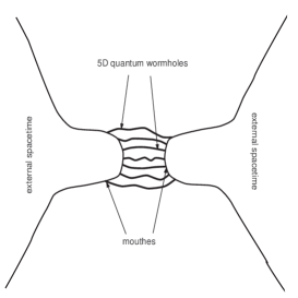
FIG. 1.: The wormhole with a quantum throat. The cloud of QWHs can be considered as the quantum throat.

To describe these QWHs we introduce a spinor field. In fact the spinor field is used for some approximate and effective description of QWHs as we are not able to do it by a direct way. Here we would like to offer the following model of the spacetime foam:

1. Each QWH is a solution of the 5D vacuum Einstein equations with $G_{5t},G_{5\varphi}\neq 0$ components of the metric that leads to the appearance of electric and magnetic fields. In some approximation we can neglect of all linear sizes of QWH and obtain that Smolin [3] calls as a “minimalist” wormhole. For the 4D observer each mouth look as $(\pm)$ electric charge since this mouth entraps the force lines of the electric field (see Fig.(3)).

2. For the external observer each QWH is like to dipole and the spacetime with the foam seems as a dielectric by filled dipoles (see Fig.(2)).

3. The spacetime foam is described by a spinor field $\psi$ and the physical meaning of $\psi$ depends on an interaction term between spinor and electromagnetic fields that we shall discuss below.

4. An interaction between electromagnetic and spinor fields is nonminimal that allows us to interpret the Maxwell equations like to the electrodynamic in a continuous media.

   

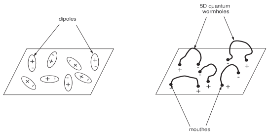
   FIG. 2.: For the 4D observer each mouth looks as a moving electric charge. This allows us in some approximation imagine the spacetime foam as a continuous media with a polarization.

II Model of the individual quantum wormhole

The model of the individual QWH is presented on the Fig.(3). In fact this is some realization of the Wheeler idea about a wormhole entrapping electric force lines. In Ref.[1] he wrote: “Along with the fluctuations in the metric there occur fluctuations in the electromagnetic field. In consequence the typical multiply connected space $\ldots$ has a net flux of electric lines of force passing through the ”wormhole”. These lines are trapped by the topology of the space. These lines give the appearance of a positive charge at one end of the wormhole and a negative charge at the other”.

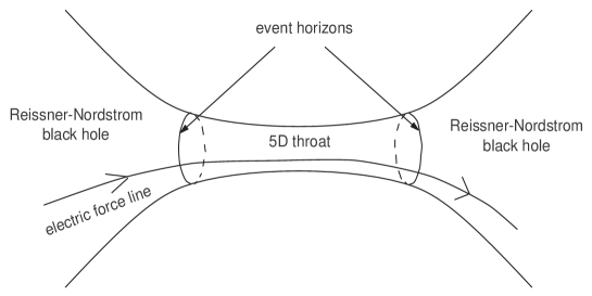
FIG. 3.: The model of the individual quantum wormhole. The whole spacetime is 5 dimensional but: in the Reissner-Nordström black hole $G_{55}=const$ and it is not varying (this is the 5D gravity in the initial Kaluza-Klein interpretation); in the 5D throat $G_{55}$ is the dynamical variable and we have 15 equations which are equivalent to 4D Einstein + Maxwell + scalar equations.

The composite wormhole on the Fig.(3) consists from two Reissner-Nordström black holes and the 5D throat inserted between them [4]. The 5D metric for this throat is

$$ds^{2}_{(5)}=-R_{0}^{2}e^{2\psi(r)}\Delta(r)\left(d\chi+\omega(r)dt+Q\cos\theta d\varphi\right)^{2}+\frac{1}{\Delta(r)}dt^{2}-dr^{2}-a(r)\left(d\theta^{2}+\sin\theta^{2}d\varphi^{2}\right),$$ (1)

where $\chi$ is the 5^th extra coordinate; $R_{0}>0$ and $Q$ are some constants. And we assume that in some approximation such QWH of spacetime foam can be presented by this manner.

The 5D Einstein equations are

$$\frac{\Delta^{\prime\prime}}{\Delta}-\frac{{\Delta^{\prime}}^{2}}{\Delta^{2}}+\frac{\Delta^{\prime}\psi^{\prime}}{\Delta}+\frac{a^{\prime}\Delta^{\prime}}{a\Delta}+R_{0}^{2}{\omega^{\prime}}^{2}\Delta^{2}e^{2\psi} = 0,$$ (2)

$$\omega^{\prime\prime}+\omega^{\prime}\left(2\frac{\Delta^{\prime}}{\Delta}+3\psi^{\prime}+\frac{a^{\prime}}{a}\right) = 0,$$ (3)

$$\frac{a^{\prime\prime}}{a}+\frac{a^{\prime}\psi^{\prime}}{a}-\frac{2}{a}+\frac{Q^{2}\Delta e^{2\psi}}{a^{2}} = 0,$$ (4)

$$\psi^{\prime\prime}+{\psi^{\prime}}^{2}+\frac{a^{\prime}\psi^{\prime}}{a}-\frac{Q^{2}\Delta e^{2\psi}}{2a^{2}} = 0,$$ (5)

$$\frac{{\Delta^{\prime}}^{2}}{\Delta^{2}}+2\frac{\Delta^{\prime}\psi^{\prime}}{\Delta}-4\frac{a^{\prime}\psi^{\prime}}{a}+\frac{4}{a}-\frac{{a^{\prime}}^{2}}{a^{2}}-R_{0}^{2}{\omega^{\prime}}^{2}\Delta^{2}e^{2\psi}-\frac{Q^{2}\Delta e^{2\psi}}{a^{2}} = 0.$$ (6)

In Ref. [5] it is shown that there is three type of solutions : the first type (wormhole-like solution) is presented on Fig.(3) with $E>H$ ($E$ and $H$ are Kaluza-Klein electric and magnetic fields), the second one is an infinite flux tube with $E=H$ and the third one is a singular solution (finite flux tube) with $E<H$. The definitions for $E$ and $H$ fields will be given later.

The longitudinal size $l_{0}$ of the WH-like solution depends on the relation between $E$ and $H$ : if $H/E\rightarrow 1$ then $l_{0}\rightarrow\infty$. Let us define an approximate solution close to points $r^{2}=r^{2}_{0}$ (where $ds^{2}(\pm r_{0})=0$). This solution we search in the form

$$\Delta \approx \Delta_{1}\left(r_{0}^{2}-r^{2}\right),$$ (7)

$$\omega \approx \frac{\omega_{1}}{r_{0}^{2}-r^{2}},$$ (8)

$$\psi \approx \frac{\psi_{3}}{6}\left(r_{0}^{2}-r^{2}\right)^{3}.$$ (9)

The solution is

$$\Delta_{1} = \pm\frac{q}{2a_{0}r_{0}},$$ (10)

$$\omega_{1} = \frac{2a_{0}r_{0}}{q},$$ (11)

$$\psi_{3} = \pm\frac{qQ^{2}}{2a_{0}^{3}r_{0}^{3}}$$ (12)

here $a_{0}=a(r=\pm r_{0})$, $q$ is some constant. It is easy to show that at the hypersurfaces $r=\pm r_{0}$ : $ds^{2}=0$. On these hypersurfaces the change of the metric signature takes place : $(+,-,-,-,-)$ by $|r|<r_{0}$ and $(-,-,-,-,+)$ by $|r|>r_{0}$. Following to Bronnikov [6] we call these two hypersurfaces as $T-$horizons.

For the definition of a Kaluza-Klein electric field we consider Eq.(3)

$$\left[\left(\omega^{\prime}\Delta^{2}e^{3\psi}\right)4\pi a\right]^{\prime}=0$$ (13)

here $4\pi a$ is the area of $S^{2}$ sphere. Comparing with the Gauss law we see that Kaluza-Klein electric field can be defined as follows

$$E_{KK}=\omega^{\prime}\Delta^{2}e^{3\psi}=\frac{q}{a}$$ (14)

here $q$ is an electric charge which is proportional to a flux of electric field. In this case the force lines of the electric field are uninterrupted and can be continued through the surfaces of matching the 5D WH-like solution and the Reissner-Nordström solution like to Fig.3. For the definition of a Kaluza-Klein magnetic field we write the following 5D Einstein equation

$$R_{\chi\varphi}=\frac{e^{\psi}\sqrt{\Delta}}{a^{2}\sin\theta}\frac{\partial}{\partial\theta}\biggl{(}Q\biggl{)}=0$$ (15)

and compare it with the ordinary 4D Maxwell equation

$$\frac{1}{\sqrt{-g}}\frac{\partial}{\partial x^{\mu}}\biggl{(}\sqrt{-g}F^{\varphi\mu}\biggl{)}=\frac{1}{\sin\theta}\frac{\partial}{\partial\theta}\biggl{(}\sin\theta F^{\theta\varphi}\biggl{)}=\frac{1}{\sin\theta}\frac{\partial}{\partial\theta}\biggl{(}\frac{H_{r}}{a}\biggl{)}=0$$ (16)

here $F^{\theta\varphi}=\frac{\epsilon^{\theta\varphi i}}{\sqrt{\gamma}}H_{i}$, $\varepsilon^{ijk}$ is the antisymmetrical tensor, $\gamma$ is the determinant of the 3D metric. The result is

$$H_{r}=\frac{Q\sqrt{\Delta}e^{\psi}}{a}.$$ (17)

Immediately we see that $H_{r}\rightarrow 0$ by $r\rightarrow\pm r_{0}$. The Einstein equations tell us that close to hypersurface $r=\pm r_{0}$ the Kaluza-Klein magnetic field can not have any influence on the gravity as the following term in Eq’s (4), (5) and (6) tends to zero

$$H_{r}^{2}=\frac{Q^{2}\Delta e^{2\psi}}{a^{2}}\rightarrow 0\quad\text{by}\quad r\rightarrow\pm r_{0}.$$ (18)

It means that the WH-like solutions near to these hypersurfaces are identical to the solution without the magnetic field. The external 4D observer sees that the force lines of magnetic field do not cross the event horizon for such composite WH. Another words each of QWH is like to moving electric charge but not a magnetic charge.

On these $T-$horizons we should match:

• the flux of the 4D electric field (defined by the Maxwell equations) with the flux of the 5D electric field defined by $R_{5t}=0$ Kaluza-Klein equation.

• the area of the Reissner-Nordström event horizon with the area of the $T-$hprizon.

It is necessary to note that both solutions (Reissner-Nordström black hole and 5D throat) have only two integration constants and on the event horizon takes place an algebraic relation between these 4D and 5D integration constants. Another explanation of the fact that we use only two joining condition is the following (see Ref.[7] for the more detailed explanations): in some sense on the event horizon holds a “holography principle”. This means that in the presence of the event horizon the 4D and 5D Einstein equations lead to a reduction of the amount of initial data. For example the Einstein - Maxwell equations for the Reissner-Nordström metric

$$ds^{2} = \Delta dt^{2}-\frac{dr^{2}}{\Delta}-r^{2}\left(d\theta^{2}+\sin^{2}d\varphi^{2}\right),$$ (19)

$$A_{\mu} = \left(\omega,0,0,0)\right)$$ (20)

(where $A_{\mu}$ is the electromagnetic potential, $\kappa$ is the gravitational constant) can be written as

$$-\frac{\Delta^{\prime}}{r}+\frac{1-\Delta}{r^{2}} = \frac{\kappa}{2}{\omega^{\prime}}^{2},$$ (21)

$$\omega^{\prime} = \frac{q}{r^{2}}.$$ (22)

For the Reissner - Nordström black hole the event horizon is defined by the condition $\Delta(r_{g})=0$, where $r_{g}$ is the radius of the event horizon. Hence in this case we see that on the event horizon

$$\Delta^{\prime}_{g}=\frac{1}{r_{g}}-\frac{\kappa}{2}r_{g}{\omega^{\prime}_{g}}^{2},$$ (23)

here (g) means that the corresponding value is taken on the event horizon. Thus, Eq. (21), which is the Einstein equation, is the first-order differential equation in the whole spacetime $(r\geq r_{g})$. The condition (23) tells us that the derivative of the metric on the event horizon is expressed through the metric value on the event horizon. This is the same what we said above: the reduction of the amount of initial data takes place by such a way that we have only two integration constants (mass $m$ and charge $e$ for the Reissner-Nordström solution and $q$ and $r_{0}$ for the 5D throat).

III Spacetime Foam and Spinor Fields

On the next approximation step we want to neglect with a cross section and longitudinal length of the 5D throat. In the result each QWH looks as an identification of two points, see Fig.4

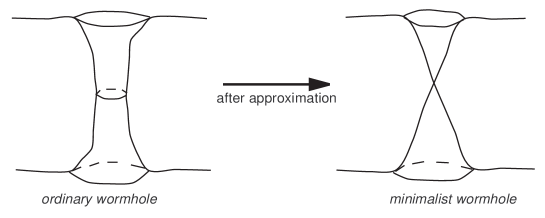
FIG. 4.: The minimalist wormhole.

Following to Smolin [3] we introduce an operator $\hat{A}^{ab}(x^{\mu},y^{\mu})$ describing a quantum state in which the space with two points $x$ and $y$ fluctuates between two possibilities : points $(x,y)$ either are pasted together or not. In fact this operator describes an undeterminacy connected with the creation/annihilation of a wormhole. Smolin calls such wormhole as a minimalist wormhole. The minimalist wormhole can be received from the above-mentioned composite wormhole if we neglect the linear sizes of 5D throat, i.e. shrink their to a point (see, Fig.4). We demand that this operator $\hat{A}^{ab}(x,y)$ should have the following property

$$\hat{A}^{ab}(x,y)=\theta^{a}(x)\theta^{b}(y)$$ (24)

$a,b$ are some indices which will be determine later. Of coarse for the definition of $\theta^{a}(x)$ we should have some additional equation for this quantity. Smolin’s definition is

$$\hat{A}^{ab}(x,y) = \epsilon^{ab}\hat{A}(x,y)=\theta^{a}(x)\theta^{b}(y),$$ (25)

$$\left(\hat{A}(x,y)\right)^{2} = 0$$ (26)

here $a,b$ are the spinor indices and $\theta^{a}(x)$ is a spinor, $\epsilon^{12}=-\epsilon^{21}=1,\epsilon^{11}=\epsilon^{22}=0$. We would like to say that it can be various definitions : a dynamical definition with field equations is given in section IV and the definition for which $\theta^{a}(x)=\theta^{a}=const$ will be given in section V.

IV An effective model of the spacetime foam

In this case the quantity $\theta^{a}(x)$ is a spinor field $\psi^{\alpha}(x)=\theta^{\alpha}(x)$ ($a=\alpha$ is the spinor index) and we determine $\psi(x)$ dynamically by means of some field equations for $\psi(x)$.

It is well known that gauge fields naturally appears in multidimensional gravities [8], [9], [10] as some components of the multi-bein. But for the spinor field it is not the case. The spinor field in 4D and 5D spacetimes can have different interaction with gauge fields. For the 4D case the interaction term in Lagrangian is minimal $(i\bar{\psi}A_{\mu}\gamma^{\mu}\psi$, $\mu$ is the 4D index) but for the second case it can be $(i\bar{\psi}F_{AB}\gamma^{A}\gamma^{B}\psi)$ or $(iF_{AB}\bar{\psi}^{A}\psi^{B})$ (here $\psi^{A}$ is the Rarita-Schwinger spinor, $A,B$ are the 5D indices) or something like this.

We will consider the 5D Kaluza-Klein theory + torsion + spinor field with the 5D metric

$$ds^{2}=-\left(d\chi+A_{\mu}dx^{\mu}\right)^{2}+g_{\mu\nu}dx^{\mu}dx^{\nu}$$ (27)

In this case (according to the initial interpretation of the Kaluza-Klein gravity with $G_{55}=const$) we have the electromagnetic potential $A_{\mu}$ and the 4D metric $g_{\mu\nu}$. The Lagrangian for this theory is

$${\cal L} = \sqrt{-G}\left\{-\frac{1}{2k}\left(R^{(5)}-S_{ABC}S^{ABC}\right)+\right.$$ (29)

$$\left.\frac{\hbar c}{2}\left\{i\bar{\psi}\left[\gamma^{C}\left(\partial_{C}-\frac{1}{4}\omega_{\bar{A}\bar{B}C}\gamma^{[\bar{A}}\gamma^{\bar{B}]}-\frac{1}{4}S_{\bar{A}\bar{B}C}\gamma^{[\bar{A}}\gamma^{\bar{B}]}\right)-\frac{mc}{i\hbar}\right]\psi+h.c.\right\}\right\}$$

where $G$ is the determinant of the 5D metric, $R^{(5)}$ is the 5D scalar curvature, $S_{ABC}$ is the antisymmetrical torsion tensor, $A,B,C$ are the 5D world indexes, $\bar{A},\bar{B},\bar{C}$ are the 5-bein indexes, $\gamma^{B}=h^{B}_{\bar{A}}\gamma^{\bar{A}}$, $h^{B}_{\bar{A}}$ is the 5-bein, $\gamma^{\bar{A}}$ are the 5D $\gamma$ matrixes with usual definitions $\gamma^{\bar{A}}\gamma^{\bar{B}}+\gamma^{\bar{B}}\gamma^{\bar{A}}=2\eta^{\bar{A}\bar{B}}$, $\eta^{\bar{A}\bar{B}}=(+,-,-,-,-)$ is the signature of the 5D metric; $[]$ means the antisymmetrization, $\hbar$, $c$ and $m$ are the usual constants. The most important for us is the choice of a spinor $\psi$ which will approximately describe the spacetime foam as it was mentioned in the section III : i.e. $\psi^{\alpha}(x)=\theta^{\alpha}(x)$. It is very important to note that in the context of this section we have some dynamical equations for the $\theta^{\alpha}(x)=\psi^{\alpha}(x)$ (it is convenient to use the usual designation $\psi$ for the fermion field). We should note that all physical fields in Lagrangian (29) must be quantum operators but on the first approximation step we change their by classical fields. After dimensional reduction we have

$${\cal L} = \sqrt{-g}\left\{-\frac{1}{2k}\left(R+\frac{1}{4}F_{\alpha\beta}F^{\alpha\beta}\right)+\right.$$ (31)

$$\left.\frac{\hbar c}{2}\left[i\bar{\psi}\left(\gamma^{\mu}\tilde{\nabla}_{\mu}-\frac{1}{8}F_{\bar{\alpha}\bar{\beta}}\gamma^{\bar{5}}\gamma^{[\bar{\alpha}}\gamma^{\bar{\beta}]}-\frac{1}{4}l^{2}_{Pl}\left(\gamma^{[\bar{A}}\gamma^{\bar{B}}\gamma^{\bar{C}]}\right)\left(i\bar{\psi}\gamma_{[\bar{A}}\gamma_{\bar{B}}\gamma_{\bar{C}]}\psi\right)-\frac{mc}{i\hbar}\right)\psi+h.c.\right]\right\}$$

$$S^{\bar{A}\bar{B}\bar{C}} = 2l^{2}_{Pl}\left(i\bar{\psi}\gamma^{[\bar{A}}\gamma^{\bar{B}}\gamma^{\bar{C}]}\psi\right)$$ (32)

where $g$ is the determinant of the 4D metric, $R$ is the 4D scalar curvature, $F_{\alpha\beta}=\partial_{\alpha}A_{\beta}-\partial_{\beta}A_{\alpha}$ is the Maxwell tensor, $A_{\mu}=h^{\bar{5}}_{\mu}$ is the electromagnetic potential, $\alpha,\beta,\mu$ are the 4D world indexes, $\bar{\alpha},\bar{\beta},\bar{\mu}$ are the 4D vier-bein indexes, $h^{\bar{\mu}}_{\nu}$ is the vier-bein, $\gamma^{\bar{\mu}}$ are the 4D $\gamma$ matrixes with usual definitions $\gamma^{\bar{\mu}}\gamma^{\bar{\nu}}+\gamma^{\bar{\nu}}\gamma^{\bar{\mu}}=2\eta^{\bar{\mu}\bar{\nu}}$, $\eta^{\bar{\mu}\bar{\nu}}=(+,-,-,-)$ is the signature of the 4D metric. Varying with respect to $g_{\mu\nu}$, $\bar{\psi}$ and $A_{\mu}$ leads to the following equations

$$R_{\mu\nu}-\frac{1}{2}g_{\mu\nu}R=\frac{1}{2}\left(-F_{\mu\alpha}F_{\nu}^{\alpha}+\frac{1}{4}g_{\mu\nu}F_{\alpha\beta}F^{\alpha\beta}\right) + 4l^{2}_{Pl}\left[\left(i\bar{\psi}\gamma_{\mu}\tilde{\nabla}_{\nu}\psi+i\bar{\psi}\gamma_{\nu}\tilde{\nabla}_{\mu}\psi\right)+h.c.\right]-$$ (33)

$$2l^{2}_{Pl}\left[F_{\mu\alpha}\left(i\bar{\psi}\gamma^{\bar{5}}\gamma_{[\nu}\gamma^{\alpha]}\psi\right)+F_{\nu\alpha}\left(i\bar{\psi}\gamma^{\bar{5}}\gamma_{[\mu}\gamma^{\alpha]}\psi\right)\right] - 2g_{\mu\nu}l^{4}_{Pl}\left(i\bar{\psi}\gamma^{[\bar{A}}\gamma^{\bar{B}}\gamma^{\bar{C}]}\psi\right)\left(i\bar{\psi}\gamma_{[\bar{A}}\gamma_{\bar{B}}\gamma_{\bar{C}]}\psi\right),$$ (34)

$$D_{\nu}H^{\mu\nu}=0,\,H^{\mu\nu}=F^{\mu\nu}+\tilde{F}^{\mu\nu};\,\tilde{F}^{\mu\nu} = 4l^{2}_{Pl}\left(i\bar{\psi}\gamma^{\bar{5}}\gamma^{[\mu}\gamma^{\nu]}\psi\right)=4l^{2}_{Pl}E^{\mu\nu\alpha\beta}\left(i\bar{\psi}\gamma_{[\alpha}\gamma_{\beta]}\psi\right),$$ (35)

$$i\gamma^{\mu}\tilde{\nabla}_{\mu}\psi-\frac{1}{8}F_{\bar{\alpha}\bar{\beta}}\left(i\gamma^{\bar{5}}\gamma^{[\bar{\alpha}}\gamma^{\bar{\beta}]}\psi\right) - \frac{1}{2}l^{2}_{Pl}\left(i\gamma^{[\bar{A}}\gamma^{\bar{B}}\gamma^{\bar{C}]}\psi\right)\left(i\bar{\psi}\gamma_{[\bar{A}}\gamma_{\bar{B}}\gamma_{\bar{C}]}\psi\right)=0,$$ (36)

$$\tilde{\nabla}_{\mu} = \partial_{\mu}-\frac{1}{4}\omega_{\bar{a}\bar{b}\mu}\gamma^{[\bar{a}}\gamma^{\bar{b}]}$$ (37)

where $\tilde{\nabla}_{\mu}$ is the 4D covariant derivative of the spinor field without torsion, $\omega_{\bar{a}\bar{b}\mu}$ is the 4D Ricci coefficients without torsion, $E^{\mu\nu\alpha\beta}$ is the 4D absolutely antisymmetric tensor. The most interesting for us is the Maxwell equation (35) which permits us to discuss the physical meaning of the spinor field. We would like to show that this equation in the given form is similar to the electrodynamic in the continuous media. Let we remind that for the electrodynamic in the continuous media two tensors $\bar{F}^{\mu\nu}$ and $\bar{H}^{\mu\nu}$ are introduced [11] for which we have the following equations system (in the Minkowski spacetime)

$$\bar{F}_{\alpha\beta,\gamma}+\bar{F}_{\gamma\alpha,\beta}+\bar{F}_{\beta\gamma,\alpha} = 0,$$ (38)

$$\bar{H}^{\alpha\beta}_{,\beta} = 0$$ (39)

and the following relations between these tensors

$$\bar{H}_{\alpha\beta}u^{\beta} = \varepsilon\bar{F}_{\alpha\beta}u^{\beta},$$ (40)

$$\bar{F}_{\alpha\beta}u_{\gamma}+\bar{F}_{\gamma\alpha}u_{\beta}+\bar{F}_{\beta\gamma}u_{\alpha} = \mu\left(\bar{H}_{\alpha\beta}u_{\gamma}+\bar{H}_{\gamma\alpha}u_{\beta}+\bar{H}_{\beta\gamma}u_{\alpha}\right)$$ (41)

where $\varepsilon$ and $\mu$ are the dielectric and magnetic permeability respectively, $u^{\alpha}$ is the 4-vector of the matter. For the rest media and in the 3D designation we have

$$\varepsilon\bar{E}_{i} = \bar{E}_{i}+4\pi\bar{P}_{i}=\bar{D}_{i},\quad\mbox{where}\quad\bar{E}_{i}=\bar{F}_{0i},\quad\bar{D}_{0i}=\bar{H}_{0i},$$ (42)

$$\mu\bar{H}_{i} = \bar{H}_{i}+4\pi\bar{M}_{i}=\bar{B}_{i},\quad\mbox{where}\quad\bar{B}_{i}=\epsilon_{ijk}\bar{F}^{jk},\quad\bar{H}_{i}=\epsilon_{ijk}\bar{H}^{jk},$$ (43)

where $P_{i}$ is the dielectric polarization and $M_{i}$ is the magnetization vectors, $\epsilon_{ijk}$ is the 3D absolutely antisymmetric tensor. Let us rewrite the definition in Eq.(35) in the following form

$$E_{i}+\tilde{E}_{i} = D_{i}\quad\mbox{where }\quad E_{i}=F_{0i},\quad\tilde{E}_{i}=\tilde{F}_{0i},\quad D_{i}=H_{0i}$$ (44)

$$B_{i}+\tilde{B}_{i} = H_{i}\quad\mbox{where}\quad B_{i}=\epsilon_{ijk}F^{jk},\quad\tilde{B}_{i}=\epsilon_{ijk}\tilde{F}^{jk},\quad H_{i}=\epsilon_{ijk}H^{jk}.$$ (45)

Comparing these definitions with (42), (43) immediately we see that the following notations can be introduced

$$\tilde{E}_{i}=4l^{2}_{Pl}\epsilon_{ijk}\left(i\bar{\psi}\gamma^{[j}\gamma^{k]}\psi\right)$$ (46)

is the polarization vector of the spacetime foam and

$$\tilde{B}_{i}=-4l^{2}_{Pl}\epsilon_{ijk}\left(i\bar{\psi}\gamma^{\bar{5}}\gamma^{[j}\gamma^{k]}\psi\right)$$ (47)

is the magnetization vector of the spacetime foam.

The physical reason for this is : each QWH is like to a moving dipole (see Fig.(2)) which produces microscopical electric and magnetic fields.

V Supergravity as a possible model of the spacetime foam

Now we would like to consider the another possible interpretation of $\theta^{a}(x)$. In this case (in contrast to section IV) we determine the quantity $\theta^{a}(x)$ by a non-dynamic way : introducing some algebraic equation (48) for $\theta$. Let the operator $\hat{A}^{ab}(x,y)$ introduced in the section III satisfies to the following equation

$$\hat{A}^{ab}(x,y)\hat{A}_{ab}(x,y)=0.$$ (48)

The solution of Eq.(48) we search in the form

$$\hat{A}^{ab}(x,y)=\theta^{a}(x)\theta^{b}(y).$$ (49)

After substitution in Eq.(48) we have

$$\theta^{a}(x)\theta^{b}(y)\theta_{a}(x)\theta_{b}(y)=0.$$ (50)

Like to section III we have two simplest solution. The first solution is

$$a = \alpha,\;b=\beta,\;(\alpha,\beta=1,2),$$ (51)

$$\hat{A}^{\alpha\beta}(x,y) = \theta^{\alpha}(x)\theta^{\beta}(y).$$ (52)

$\theta^{\alpha}$ is an undotted spinor of $(\frac{1}{2},0)$ representation of Sl(2,C) group.

$$\theta^{\alpha}(x) = \theta^{\alpha}(y)=\theta^{\alpha}=const,$$ (53)

$$\theta^{\alpha}\theta^{\beta} = -\theta^{\beta}\theta^{\alpha};\qquad\alpha\neq\beta,$$ (54)

$$\left(\theta^{\alpha}\right)^{2} = 0.$$ (55)

The second solution is similar : $\alpha\rightarrow\dot{\alpha}$ and $\beta\rightarrow\dot{\beta}$

$$a = \dot{\alpha},\;b=\dot{\beta},\;(\dot{\alpha},\dot{\beta}=1,2),$$ (56)

$$\hat{A}^{\dot{\alpha}\dot{\beta}}(x,y) = \bar{\theta}^{\dot{\alpha}}(x)\bar{\theta}^{\dot{\beta}}(y),$$ (57)

$$\bar{\theta}^{\dot{\alpha}}(x) = \bar{\theta}^{\dot{\alpha}}(y)=\bar{\theta}^{\dot{\alpha}}=const,$$ (58)

$$\bar{\theta}^{\dot{\alpha}}\bar{\theta}^{\dot{\beta}} = -\bar{\theta}^{\dot{\beta}}\bar{\theta}^{\dot{\alpha}};\qquad\dot{\alpha}\neq\dot{\beta},$$ (59)

$$\left(\bar{\theta}^{\dot{\alpha}}\right)^{2} = 0.$$ (60)

In this case $\bar{\theta}^{\dot{\alpha}}$ is a dotted spinor of $(0,\frac{1}{2})$ representation. Such two-valuedness compels us to introduce both possibilities : $\theta=\{\theta^{\alpha},\bar{\theta}^{\dot{\alpha}}\}$.

Like to Smolin [3] we would like to introduce an infinitesimal operator $\delta\hat{B}(x^{\mu}\rightarrow z^{\mu}=x^{\mu}+\delta x^{\mu})$ of a displacement of the wormhole mouth

$$\delta\hat{B}(x^{\mu} \rightarrow z^{\mu})\hat{A}^{\gamma\delta}(y^{\mu},x^{\mu})=\hat{A}^{\gamma\delta}(y^{\mu},z^{\mu}),$$ (61)

$$\hat{A}^{\gamma\delta}(y^{\mu},x^{\mu}) = \theta^{\gamma}\theta^{\delta},$$ (62)

$$\hat{A}^{\gamma\delta}(y^{\mu},z^{\mu}) = {\theta^{\prime}}^{\gamma}{\theta^{\prime}}^{\delta}=\left(\theta^{\gamma}+\varepsilon^{\gamma}\right)\left(\theta^{\delta}+\varepsilon^{\delta}\right)\approx\theta^{\gamma}\theta^{\delta}+\varepsilon^{\gamma}\theta^{\delta}-\varepsilon^{\delta}\theta^{\gamma}$$ (63)

here $\varepsilon^{\alpha}$ is an infinitesimal Grassmannian number. Therefore we have the following equation for the definition of $\delta\hat{B}(x^{\mu}\rightarrow z^{\mu})$ operator

$$\delta\hat{B}\left(x^{\mu}\rightarrow z^{\mu}\right)\theta^{\gamma}\theta^{\delta}=\theta^{\gamma}\theta^{\delta}+\varepsilon^{\gamma}\theta^{\delta}-\varepsilon^{\delta}\theta^{\gamma}.$$ (64)

This equation has the following solution [13]

$$\delta\hat{B}\left(x^{\mu}\rightarrow z^{\mu}\right)=1+\varepsilon^{\alpha}\frac{\partial}{\partial\theta^{\alpha}}-i\varepsilon^{\alpha}\sigma^{\mu}_{\alpha\dot{\beta}}\bar{\theta}^{\dot{\beta}}\partial_{\mu}-\bar{\varepsilon}^{\dot{\alpha}}\frac{\partial}{\partial\bar{\theta}^{\dot{\alpha}}}+i\theta^{\alpha}\sigma^{\mu}_{\alpha\dot{\beta}}\bar{\varepsilon}^{\dot{\beta}}\partial_{\mu}.$$ (65)

This allows us to say that $\theta=\{\theta^{\alpha},\theta^{\dot{\alpha}}\}$ are the Grassmanian numbers which we should use as some additional coordinates for the description of the spacetime foam. In this approach the superspace gravity with the anticommuting coordinates $\theta$ describes in some approximation the spacetime foam.

VI Conclusions

Thus, here we have proposed the approximate model for the description of the spacetime foam. This model is based on the assumption that the whole spacetime is 5 dimensional but $G_{55}$ is the dynamical variable only in the QWHs. In this case 5D gravity has the solution which we have used as a model of the individual quantum wormhole. In the approximation when the 5D throat of each QWH is contracted to a point the spacetime foam can be approximately described by a spinor field or Grassmanian anticommuting coordinates on the superspace.

Such model leads to the very interesting experimental consequences. We see that the spacetime foam has 5D structure and it connected with the electric field. This observation allows us to presuppose that the very strong electric field can open a door into 5 dimension! The question is: as is great should be this field ? The electric field $E_{i}$ in the CGSE units and $e_{i}$ in the “geometrized” units can be connected by formula

$$e_{i} = \frac{G^{1/2}}{c^{2}}E_{i}=\left(2.874\times 10^{-25}\;cm^{-1}/gauss\right)E_{i},$$ (66)

$$\left[e_{i}\right] = cm^{-1},\quad\left[E_{i}\right]=V/cm$$ (67)

As we see the value of $e_{i}$ is defined by some characteristic length $l_{0}$. It is possible that $l_{0}$ is a length of the $5^{th}$ dimension. If $l_{0}=l_{Pl}$ then $E_{i}\approx 10^{57}V/cm$ and this field strength is in the Planck region, and is will beyond experimental capabilities to create. But if $l_{0}$ has a different value it can lead to much more realistic scenario for the experimental capability to open door into $5^{th}$ dimension.

Another conclusion of this work is that : the supergravity theories can be considered as approximative and effective models of the spacetime foam.

VII Acknowledgment

I am grateful for financial support from the Georg Forster Research Fellowship of the Alexander von Humboldt Foundation and H.-J. Schmidt for an invitation to Potsdam University.

REFERENCES

• [1] J. Wheeler, Ann. of Phys., 2, 604(1957).
• [2] V. Dzhunushaliev, “Wormhole with Quantum throat”, gr-qc/0005008, to be published in Grav. Cosmol.
• [3] L. Smolin, “Fermions and topology”, gr-qc/9404010.
• [4] V. Dzhunushaliev, Mod. Phys. Lett. A 13, 2179 (1998).
• [5] V. Dzhunushaliev and D. Singleton, Phys. Rev. D 59, 064018 (1999).
• [6] Bronnikov K., Int.J.Mod.Phys. D4, 491(1995), Grav. Cosmol., 1, 67(1995).
• [7] V. D. Dzhunushaliev, Int. J. Mod. Phys., 9, 551(2000), gr-qc/9907086.
• [8] A. Salam and J. Strathdee, Ann. Phys. 141, 316 (1982).
• [9] R. Percacci, J. Math. Phys. 24, 807 (1983).
• [10] R. Coquereaux and A. Jadczyk, Commun. Math. Phys. 90, 79 (1983).
• [11] L.D. Landau and E.M. Lifshitz, “Electrodynamics of Continuous Media , (Pergamon Press, Oxford - London - New Jork - Paris, 1960).
• [12] S. Ferrara and P. V. Nieuwenhuizen, Phys. Rev. Lett. 37, 1669 (1976).
• [13] V. Dzhunushaliev, “A Geometrical Interpretation of Grassmannian Coordinates”, hep-th/0104129.