Black Hole Critical Phenomena Without Black Holes

Abstract

Studying the threshold of black hole formation via numerical evolution has led to the discovery of fascinating nonlinear phenomena. Power-law mass scaling, aspects of universality, and self-similarity have now been found for a large variety of models. However, questions remain. Here I briefly review critical phenomena, discuss some recent results, and describe a model which demonstrates similar phenomena without gravity.

1. Introduction

The discovery of black hole critical behavior represents an important example of the power of numerical computation in physics. The phenomena discovered were completely unpredicted and unexpected prior to the numerical work of Choptuik  [?].

In this Proceedings, I briefly review critical phenomena before describing some research of my colleagues and me. The field and its understanding have grown quickly, and this review is necessarily limited in its scope. The choice of topics is thus biased towards what I have done and follows closely my talk. I therefore try to retain some of the informality of a talk omitting detailed discussion of important topics such as casting the equations of general relativity as an evolution problem and the numerical solution of those equations. Also, a couple excellent reviews are available  [?,?], and so I attempt here to give only enough detail to equip and interest the reader in the research following. The title of this work is explained in Section 3. 3.3. I conclude by mentioning some important and general open questions and directions within the field of critical behavior.

2. Black Hole Critical Phenomena

2.1 The Space of Solutions

When a sufficiently energetic configuration of matter finds itself in a small enough region a black hole forms from the inevitable gravitational attraction. Lacking sufficient energy, such a configuration fails to produce a black hole, instead finding some other end state such as a star or dispersing altogether. Were we engineers with advanced technology, we might attempt to find that critical amount of energy necessary to form a black hole.

However, despite some fears to the contrary, such technology does not exist, so instead we investigate this critical regime numerically. The first step is to pick a matter source to consider. By this time, quite a variety of sources have been considered, but here I will start with the relatively simple case of a single scalar field $\psi$ which happens to be the first case to have been considered  [?].

Given some initial condition, the goal is to be able to determine whether or not the configuration forms a black hole. To do so, we need evolution equations for the scalar field which come from varying an appropriate action $S$ which couples the scalar field to gravity

$$S=\int d^{4}x\sqrt{-g}\Bigl{[}R-\psi_{,\mu}\psi^{,\mu}\Bigr{]}$$ (1)

where $\sqrt{-g}d^{4}x$ is the appropriate volume element, $R$ is the curvature scalar, and $\psi_{,\mu}$ denotes the partial derivatives of $\psi$. The construction of a numerical method with which to evolve the gravitationally coupled scalar field is certainly non-trivial, but is described in detail elsewhere.

Being able to determine whether a certain configuration of scalar field forms a black hole, the next goal is to examine the configuration space of the model. In other words, we would like to picture the space of all possible initial configurations of scalar field and which configurations form black holes and which disperse (the only two options in this model). The problem in picturing such a space is that it is infinite dimensional (imagine the space formed by specifying the scalar field at every point in real space).

To circumvent this difficulty, we can instead parametrize the scalar field $\psi(r,0)$ at the initial time by assuming a Gaussian form, so that

$$\psi(r,0)=Ae^{\left(r-R_{0}\right)^{2}/\delta^{2}}$$ (2)

in terms of real constants $A,R_{0},\delta$. The time derivative $\dot{\psi}(r,0)$ at the initial time must also be specified, but we can choose to have it vanish. The configuration space now has only the three dimensions corresponding to the possible values of the three constants. However, we go a step further by fixing two of the constants, say $R_{0}$ and $\delta$. We now have a family of initial data with one free parameter $A$. We could consider other one parameter families, and so we generically call the single free parameter $p$ (so here $p=A$).

Have we lost something in this simplification of using one parameter families? It turns out that we have not, which we will see later by considering a variety of such families.

To complete our map of the configuration space, we need now only determine for which values of $p$ the configuration evolves into a black hole. As intuition might suggest, for large values of $p$ black holes do form and for small values the scalar field disperses. We are now in a position to picture the configuration space which I sketch in Fig. 1.

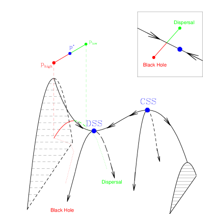
Figure  1.: Schematic of Configuration Space. Evolutions which start from initial configurations on the near side of the ridge form black holes. Those configurations lying on the far side simply disperse. The critical regime lies on the ridge which separates these two end states. The inset shows a bird’s eye view looking down on the saddle point.

Fig. 1 shows schematically a section of some generic two-dimensional (i.e. two parameter) configuration space. The third dimension (say $z$) represents loosely an effective potential which describes the fate of the configurations ($x$,$y$). Hence, initial configurations on the near side of the ridge ultimately evolve to form black holes while those configurations on the far side disperse. In general, a one parameter family is represented in this schematic as a line parameterized by $p$ which crosses the ridge somewhere, an example of which is shown.

This configuration space then reveals two end states (black hole and dispersal) which in the jargon of nonlinear dynamics are called attractors because trajectories nearby are attracted to them. These two attractors occur in their respective basins of attraction defining the regions in configuration space which are attracted to each end state. The critical region of this configuration space is then the boundary between these two end states (i.e. the ridge in the sketch of Fig. 1). One aspect of this schematic to keep in mind is that evolutions do not stay in this simplified space of initial configurations; the schematic is meant only to help picture general features of initial data, namely to what end state they evolve.

Stepping back from the abstractness for a moment, consider the actual process of studying the critical regime. A family of initial data is chosen and then an initial value of the parameter $p$. This initial data is then evolved and its final state determined. Say a black hole forms. Then this value of the parameter becomes the high value $p_{\rm high}$ and a smaller value of $p$ is chosen. Say the evolution for this $p$ corresponds to dispersal. Then this value becomes the low value $p_{\rm low}$. The interval between these two values $[p_{\rm low},p_{\rm high}]$ brackets the critical regime. To narrow the bracket, one uses a bisection search in which one evolves the average of the current bracket $p=\left(p_{\rm low}+p_{\rm high}\right)/2$ and updates the bracket according to the evolution. The iteration of such a search eventually finds a bracket in which the high and low values approach the computer’s ability to differentiate them. At this point $p_{\rm low}\approx p_{\rm high}$ and in between them somewhere is the exactly critical value of $p$ called $p^{*}$.

The above search essentially explores the region of configuration space near the ridge. What happens in this regime is the subject of black hole critical phenomena.

2.2 Phenomena Occurring in the Critical Regime

As the search is continued, a certain solution, the critical solution, corresponding to $p\rightarrow p^{*}$ is approached. Evolutions for $p$ near $p^{*}$ resemble the critical solution for some time, but eventually tear away from it and head for either black hole formation or dispersal. Imagine trying to balance a coin on its edge. The better balanced the coin becomes, the longer the coin “remains near” to the critical solution, that being the static state critically balanced between falling left and falling right.

In many of the cases studied, the critical solution demonstrates a type of self-similarity. Consider a general field configuration, say $\phi(r,t)$. However, let us change coordinates using $u\equiv\ln r-\ln|t|$ and $v\equiv\ln r+\ln|t|$ where the collapse time is chosen to occur at $t=0$. Solutions $\phi(u,v)$ which can be written as functions of $u$ alone

$$\phi(u,v)=\phi\left(u\right)$$ (3)

are self-similar. Such self-similar solutions are invariant under changes of scale accompanied by an appropriate change in time.

Remarkably, in the free scalar field case, the critical solution exhibits a discrete form of such a self-similarity, called discretely self-similar (DSS), in contrast to the above case called continuously self-similar (CSS). A solution which exhibits discrete self-similarity is no longer independent of $v$ but instead periodic in $v$

$$\phi\left(\ln r,\ln|t|\right)=\phi\left(\ln r\pm n\Delta,\ln|t|\pm n\Delta\right),$$ (4)

with periodicity given by the dimensionless number $\Delta$. The DSS found by Choptuik for the real scalar field has $\Delta=3.44$. The nature of this discrete self-similarity is still a bit of a mystery, but, loosely speaking the CSS can be considered some generalization of a fixed point to the infinite dimensional case while the DSS would correspond to a generalized limit cycle.

I speak here of the critical solution for the scalar field, but it is not a priori clear that there should be only one solution. In fact, one might guess that the family one picks will determine the critical solution one observes. That this is not the case demonstrates the universality of the critical solution. That is, independent of what family one picks, the critical search will always approach this same self-similar critical solution.

This universality is now understood in terms of perturbation theory  [?]. Consider linear perturbations to the exactly critical solution existing inside the full infinite-dimensional phase space of the model. The critical solution will have a number of modes, stable or unstable. The stable modes decay, and hence drive the perturbed solution back to the critical solution. However, the unstable modes are perhaps more interesting, driving the solution away from criticality.

The key point here is that the critical solution can have only one unstable mode. It is the action of this unstable mode near the critical point which drives slightly sub-critical solutions to dispersal and super-critical solutions to black hole formation. Hence, the one parameter tunes the excitation of this single unstable mode while the stable modes drive the solution towards the critical solution. Such a solution is an intermediate attractor because it is only one unstable mode away from being an attractor. Because of these dynamics, tuning similar families of initial data are driven (modulo the unstable mode) towards the same critical solution.

This picture of the perturbative modes also explains another feature of critical behavior, namely power law mass scaling of the black holes formed. As stated above, tuning of $p$ drives the excitation of the unstable mode to zero, and hence for slightly supercritical evolutions, the scale of the excitation is set by $p-p^{*}$. It can then be shown that the mass of the black holes formed by such evolutions follows a power law as

$$M\propto\left(p-p^{*}\right)^{\gamma}$$ (5)

for some constant $\gamma$ determined by the model. In the case of the free scalar field, the mass scaling exponent about the DSS is $\gamma=0.37$. The perturbative picture has successfully shown that $\gamma$ is given by the inverse of the eigenvalue of the single exponentially growing mode of the critical solution.

We consider how these solutions appear at times near to collapse. Whether CSS or DSS, the dynamics appear at smaller and smaller spatial scales which correspond to regions of arbitrarily high curvature visibly at infinity. The exactly critical solution has a naked singularity. Critical behavior thus becomes a way to find naked singularities.

The discussion above applies directly to regions of phase space in which a self-similar solution plays the role of the critical solution. In these cases, black holes form with arbitrarily small mass (for $p$ arbitrarily close to $p^{*}$), and in analogy to phase transitions with order parameter $M$, these case are called Type II. Other models not discussed here possess stationary solutions which act as critical solutions in which case the black hole formation has a finite lower limit for their mass. Such models exhibit Type I collapse.

3. Two, Three, and Four Fields

We have considered so far the simple case of just one scalar field. By now a large number of different matter models have been considered with a variety of interesting twists and turns in the picture presented above. Here I describe a few models I have studied which happen to categorize themselves by the number of scalar fields they employ. For background, I make note of a few useful resources which discuss such multiple scalar field models. Ryder discusses the real and complex scalar fields as a precursor to quantum field theory  [?]. Rajaraman discusses monopoles and charge conservation from a mathematical perspective  [?] while Vilenkin and Shellard present the standard discussion of these models in the context of topological defects  [?].

3.1 Two Fields: Generalized Complex Scalar Field

Consider a complex scalar field $F(r,t)\equiv\psi(r,t)+i\phi(r,t)$ in terms of real scalar fields $\psi$ and $\phi$ with the action

$$S=\int d^{4}x\sqrt{-g}\left(R-\frac{2|\nabla F|^{2}}{\left(1-\kappa|F|^{2}\right)^{2}}\right),$$ (6)

where $\kappa$ is a dimensionless parameter of the model. For $\kappa=0$, the model reduces to a free complex scalar field while for general $\kappa$ the model is the nonlinear sigma model with target manifold corresponding to surfaces of constant curvature $-\kappa$. For negative values of $\kappa$ the target space is $S^{2}$ corresponding to the group $SO(2)$  [?].

For $\kappa=0$ the model corresponds to the free complex scalar field for which the $\Delta=3.44$ DSS is the known attracting critical solution. However, Hirschmann and Eardley study this model and find that if $\kappa$ is increased above $\kappa\approx 0.075$ a bifurcation occurs such that a CSS becomes the attracting critical solution  [?]. This bifurcation occurs in a region of parameter space equivalent to that of a free scalar field coupled to Brans-Dicke gravity, and the bifurcation has been confirmed in that model  [?].

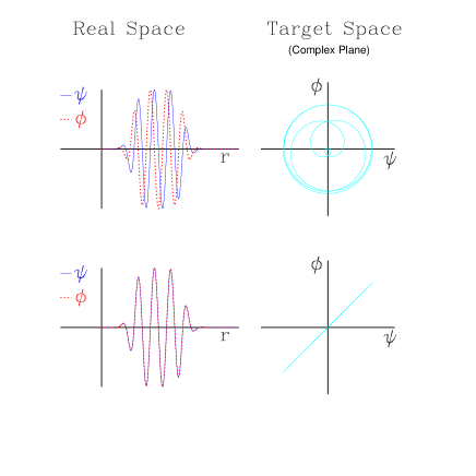
Figure  2.: Aspects of the spiral initial data. On top is the spiral data Eq. (8) for $\Delta\varphi=0$ and on bottom is that for $\Delta\varphi=-\pi/2$. On the left are shown the real and imaginary parts of the complex field $F(r,0)$ as functions of space. On the right is shown $F(r,0)$ in the complex plane.

What a surprise then to find that the above results fail to hold with a certain family of initial data that I call spiral data. I consider initial data for $F(r,t)$ such that the real and imaginary parts are

$$\psi(r,0) = p~{}f(r)\cos(\omega r+\Delta\varphi)$$ (7)

$$\phi(r,0) = p~{}f(r)\sin(\omega r),$$ (8)

where $p$ and $\Delta\varphi$ are real constants and the function $f(r)$ serves as an envelope smoothly approaching zero for large and small $r$. For simplicity of some of these arguments, I assume that the initial time derivatives of the fields vanish.

Choosing Eq. (8) with $\Delta\varphi=0$ and tuning $p$ finds the CSS critical solution for $\kappa=0$ despite the fact that the CSS has multiple unstable modes (and hence is not an intermediate attractor) for $\kappa\mathrel{\mathchoice{\lower 3.0pt\vbox{\halign{$\m@th\displaystyle\hfill#\hfil$\cr<\crcr\sim\crcr}}}{\lower 3.0pt\vbox{\halign{$\m@th\textstyle\hfill#\hfil$\cr<\crcr\sim\crcr}}}{\lower 3.0pt\vbox{\halign{$\m@th\scriptstyle\hfill#\hfil$\cr<\crcr\sim\crcr}}}{\lower 3.0pt\vbox{\halign{$\m@th\scriptscriptstyle\hfill#\hfil$\cr<\crcr\sim\crcr}}}}0.075$. Similarly, fixing $\Delta\varphi=-\pi/2$ and tuning $p$ finds the DSS critical solution for $\kappa\mathrel{\mathchoice{\lower 3.0pt\vbox{\halign{$\m@th\displaystyle\hfill#\hfil$\cr>\crcr\sim\crcr}}}{\lower 3.0pt\vbox{\halign{$\m@th\textstyle\hfill#\hfil$\cr>\crcr\sim\crcr}}}{\lower 3.0pt\vbox{\halign{$\m@th\scriptstyle\hfill#\hfil$\cr>\crcr\sim\crcr}}}{\lower 3.0pt\vbox{\halign{$\m@th\scriptscriptstyle\hfill#\hfil$\cr>\crcr\sim\crcr}}}}0.075$ despite it not being an intermediate attractor.

To understand this behavior which would appear to go against the grain of the understanding presented above, we first consider certain aspects of this initial data as shown in Fig. 2. For $\Delta\varphi=-\pi/2$, we have $\psi(r,0)=\phi(r,0)$ which corresponds to having no charge in the initial data. That this data has no charge can be seen in two ways. First, the model has a global $U(1)$ symmetry under which the model is invariant to global rotations of $F(r,t)$ in the complex plane. Thus, we can rotate $F(r,0)$ until it becomes all real. In this case, the model is equivalent to a single scalar field which has no charge (two fields are necessary for there to be charge). Secondly, one can assess the charge of this initial data simply by looking at the area spanned in the complex plane. As shown in Fig. 2, for $\Delta\varphi=-\pi/2$ no area is spanned.

Contrast this case with the case of $\Delta\varphi=0$. In this case, the field can be expressed as $F(r,0)=f(r)\exp\left(i\omega r\right)$. In regions where the envelope function $f(r)=1$, the field configuration maximizes the area spanned in the complex plane, and hence maximizes the charge density for a given energy density  [?].

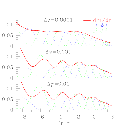
Figure  3.: The critical solution found by tuning $p$ in initial data of the form Eq. (8) for $\kappa=0$ with different values of $\Delta\varphi$. For $\Delta\varphi\rightarrow 0$, the CSS critical solution is observed where, for generic initial data, the DSS would be observed. As $\Delta\varphi$ is increased, however, the critical solution approaches the DSS.

Fig. 3 demonstrates the case of perturbing $\Delta\varphi$ away from zero. While for $\kappa=0$ with $\Delta\varphi=0$ one finds the CSS solution where one would otherwise expect to find the DSS, as $\Delta\varphi$ is perturbed, tuning $p$ quickly moves to the DSS. This indicates that the case of $\Delta\varphi=0$ is indeed quite special.

These observations suggest that changes to $\Delta\varphi$ represent tuning a second parameter. While tuning $p$ effectively tunes the mass of any black hole formed, tuning $\Delta\varphi$ tunes the charge. Hence, while the CSS has other unstable modes (a pair with complex conjugate eigenvalues) for $\kappa=0$, the spiral initial data with $\Delta\varphi=0$ represents data already tuned for maximal charge. This tuning disallows critical solutions with no charge such as the DSS.

3.2 Three Fields: Global Monopoles

Consider a triplet scalar field $\Phi^{a}$ ($a=1,2,3$) coupled to gravity with the Lagrangian

$$L=-\frac{1}{2}\Phi^{a}{}^{;\mu}\Phi^{a}{}_{;\mu}-\frac{1}{4}\lambda\left[\Big{(}\Phi^{a}\Big{)}^{2}-\eta^{2}\right]^{2}$$ (9)

where $\lambda$ is a constant representing the coupling of the potential and $\eta$ is the scale of symmetry breaking. Also assume the hedgehog ansatz for the triplet field

$$\Phi^{a}(r,\theta,\varphi,t)=f(r,t){\hat{r}}^{a},$$ (10)

with which we need only specify and evolve the field $f(r,t)$.

One interesting aspect to this model is the presence of static solutions $f_{s}(r)$, namely global monopoles. Such solutions are found with a usual shooting method by which one adjusts the value $a\equiv f_{a}^{\prime}(0)$, integrates outward to large radius, and shoots for an asymptotic boundary condition such that $f_{s}(r\rightarrow\infty)\rightarrow\eta$. Such solutions represent global monopoles of unit charge and are parametrized by $a(\eta)$.

It turns out that above a critical value $\eta=\eta_{\rm max}$ no such solutions can be found  [?]. A diagram of these solutions in terms of $\eta^{2}$ is shown in Fig. 4. As $\eta$ is increased towards the critical $\eta_{\rm max}$, the value of $a$ for which the static monopole solution is found decreases toward zero. This approach to zero represents the point at which the static monopole becomes identical to de Sitter space in which $f_{s}(r)=0$ and the symmetry-breaking potential reduces to a cosmological constant  [?].

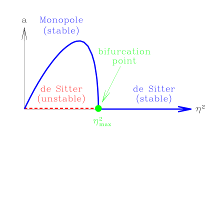
Figure  4.: Schematic of static global monopole solutions in terms of scale of symmetry breaking $\eta$ and $a$, where $a\equiv f_{s}^{\prime}(0)$. The static monopole solutions bifurcate with de Sitter space at $\eta_{\rm max}$ and stability is exchanged.

Within this model, one can consider evolving generic families of initial data specifying the scalar function $f(r,t)$. Consider first Gaussian families such as

$$f(r,0)=Ae^{\left(r-R_{0}\right)^{2}/\delta^{2}}$$ (11)

in which no monopole charge is present. With such a family, a DSS solution is observed as the critical solution, though this is not the same DSS as observed by Choptuik. Instead, I find a DSS with $\Delta=0.46$ and $\gamma=0.119$  [?].

However, a more interesting family is a Gaussian pulse as a (nonlinear) perturbation to the static monopole solution

$$f(r,0)=f_{s}(r)+Ae^{\left(r-R_{0}\right)^{2}/\delta^{2}}.$$ (12)

Observations of these families show the pulse traveling without disturbing the monopole solution. That is, the monopole persists as the pulse evolves demonstrating its stability. This stability was then explicitly confirmed via a linear analysis  [?]. Because the static monopole solutions are stable, no Type I critical behavior is expected nor observed. Instead, with the background provided by the global monopole, the usual Type II critical behavior is observed as shown in Fig. 5. The figure shows a DSS critical solution with $\Delta=0.46$ on a global monopole background. Hence, the potential is asymptotically irrelevant, as discussed in  [?].

Figure  5.: Near critical solution obtained with initial data of type Eq. (12). Shown is the function $f(r,t)$, the mass density $m^{\prime}(r,t)$, and the value of $2m(r,t)/r$ as functions of $\ln r$. In the top frame, one can see the approach of $f(r,t)$ to its background large-$r$ value $\eta=0.15$.

Maison has extended this work and found families of excited, static monopoles with multiple zeros of the Higgs field $f(r)$  [?]. These solutions appear as separate arcs (within the one shown) on the solution space schematic of Fig. 4 These solutions have an increasing number of unstable modes such that the first excited family has one unstable mode. Hence, this first excited family might occur in the context of Type I critical collapse, though such solutions have small cosmological horizons making meaningful evolutions difficult  [?].

3.3 Four Fields: Nonlinear Sigma Model

We have now looked at two scalar fields (the complex scalar field) and three fields (the global monopole), and now turn to four fields. Here again we consider a component scalar field $\Phi^{a}$ with the hedgehog ansatz, however now $a$ runs over $1,2,3,4$. With the hedgehog ansatz, the quartic field is

$$\Phi^{a}=\left(\begin{array}[]{l}\sin\chi(r,t)\sin\theta\sin\varphi\\ \sin\chi(r,t)\sin\theta\cos\varphi\\ \sin\chi(r,t)\cos\theta\\ \cos\chi(r,t)\end{array}\right)$$ (13)

in terms of another real scalar field $\chi(r,t)$. This field satisfies the same Lagrangian as the monopole case, Eq. (9), with the modifications that $a=1,2,3,4$ and gravity is not coupled to the field. We also work in the nonlinear sigma model approximation in which $\lambda$ is treated as a Lagrangian multiplier, and hence the field pays an infinite price in energy to leave the vacuum manifold. Because of this infinite price, the field is restricted to the vacuum manifold ($S^{3}$). That the ansatz Eq. (13) is everywhere and for all time on the vacuum manifold can be seen by observing that $|\Phi^{a}|=1$ (we have the freedom to set $\eta=1$ retaining full generality).

The equation of motion for $\chi(r,t)$ is then

$$\ddot{\chi}-\frac{1}{r^{2}}\left(r^{2}\chi^{\prime}\right)^{\prime}=-\frac{\sin\left(2\chi\right)}{r^{2}},$$ (14)

where a dot represents the partial derivative with respect to $t$ and a prime denotes the partial derivative with respect to $r$.

This model is not coupled to gravity and so no black holes can be formed. However, mathematicians have shown for this model that some sets of regular initial data develop singularities within some finite time  [?] while other sets of initial data are regular for all time  [?,?]. Thus the model has two end states, dispersal and singularity formation, and presumably there is some critical regime separating the two.

To investigate this region, we once again choose a one parameter family such as a Gaussian

$$\chi(r,0)=Ae^{\left(r-R_{0}\right)^{2}/\delta^{2}},$$ (15)

and consider evolutions for different $p=A$. Indeed, for small $p$ we observe the initial Gaussian pulse evolving towards large radius with no evidence of singularity formation. In other words, for small $p$, the initial data simply disperses. For large $p$ we observe unbounded growth of $\chi^{\prime}$ and $\dot{\chi}$ at the origin signaling singularity formation.

Bracketing the critical regime $p^{*}$ for the family in Eq (15), we approach a continuously self-similar solution for $\chi(r,t)$. Further for a few families of initial data with compact support, the same self-similar solution is approached indicating that the critical solution is universal within some region of parameter space  [?,?].

Figure  6.: Self-similar solutions for $\chi(r,t)$ in the nonlinear sigma model. The label $n$ labels the number of times $\chi$ crosses the line $\pi/2$ on the interval $(0,1)$ where $z\equiv-r/t$. The $n=1$ solution is the critical solution for initial data families of compact support.

It turns out that the model permits a family of self-similar solutions as found by  [?,?]. The first nine of these solutions are shown in Fig. 6. These solutions are parameterized by the number of times $\chi$ crosses $\pi/2$ between $z=0$ and $z=1$ where $z\equiv-r/t$. However, the $n=0$ solution has no unstable modes, and the other solutions become increasingly unstable, appearing to have $n$ unstable spherically symmetric modes. The $n=1$ solution, having just one unstable mode, appears to be the intermediate attractor.

Sprinkled in the discussion above have been qualifications about initial data of compact support. What if we remove such a restriction? We could then consider the collapse of so-called textures which are necessarily non-compact requiring $\chi$ to asymptote to integer multiples of $\pi$  [?]. Collapse of such global initial data is discussed in  [?], but it is not clear what behavior is contained in the critical regime.

That such a non-gravitational model shares some of the same phenomena as the black hole case suggests that many other models might contain interesting critical behavior.

4. Questions For the Future

4.1 The Future: Less symmetry

The work described above all assumes spherical symmetry. In fact, the only numerical evolutions geared towards examining critical behavior conducted in a less restrictive symmetry than spherical symmetry has been that of Abrahams and Evans  [?]. They modeled the collapse of axisymmetric gravitational waves. Moving from spherical symmetry to axisymmetry requires a large increase in numerical difficulty and sophistication which makes their work quite remarkable.

There has also been important work away from spherical symmetry using perturbation theory. The DSS critical solution for the real scalar field has been shown to have only decaying non-spherical modes, and hence is expected to be found in general collapse for initial data near spherical symmetry  [?]. Perturbation theory has also found a scaling relationship for small angular momentum of black holes formed near criticality  [?].

Much work remains though in higher dimensions. Building on the work of Abrahams and Evans, evolutions of scalar fields and other matter sources in axisymmetry might find new, non-spherically symmetric critical solutions. The scaling of angular momentum for large values can be investigated as can the stability of the known critical solutions to non-spherically symmetric modes. Because of such promise, Matt Choptuik, Eric Hirschmann and I are currently constructing an axisymmetric evolution code.

4.2 Questions

In addition to numerical work in higher dimensions, many other questions remain. That a discretely self-similar solution occurs at criticality adds to the interest of critical phenomena, but it is not clear why such a symmetry is found there. Garfinkle’s work is one of the few to start down this path, examining Einstein’s equations in terms of both a scale invariant part and an overall scale  [?]. Hopefully, more work in this direction might reveal from where the actual value of $\Delta$ is derived and what dependence it has on the matter source.

In this same vein, one wonders at the similarity between the CSS of Hirschmann and Eardley and the DSS. This particular CSS solution is self-similar, but retains a periodic nature similar to the DSS by way of a rotation in the complex plane. In other words, quantities invariant to global $U(1)$ rotations in the complex plane such as the energy density are perfectly self-similar, while phase-dependent fields such as the components of the complex field $F(r,t)$ are discretely self-similar. The energy density associated with the real or the imaginary components oscillates with changes in scale (this effect is apparent in Fig. 3). In the DSS however, these oscillating energy densities are in phase, and hence the solution as a whole is DSS, not CSS. Such a similarity would seem to indicate something rather deep in the equations.

Finally, how generic is critical behavior? Similar behavior is seen as described above in a model with no gravity, the nonlinear sigma model. Presumably there are any number of models with various attracting end states between which lies a critical surface yet to be discovered. What other symmetries might these critical solutions have? Might there be critical phenomena studied experimentally instead of numerically just as topological defects can be studied in liquid crystals?

5. Acknowledgments

I would like to thank my collaborators M.W. Choptuik, E.W. Hirschmann, J. Isenberg, and D. Maison. I would also like to acknowledge the support of NSF PHY-9900644.

REFERENCES

- [1] M.W. Choptuik, “Universality and Scaling in Gravitational Collapse of a Massless Scalar Field,” Phys. Rev. Lett. 70, 9-12 (1993).
- [2] M.W. Choptuik, “The (Unstable) threshold of black hole formation,” gr-qc/9803075.
- [3] C. Gundlach, “Critical phenomena in gravitational collapse - Living Reviews,” gr-qc/0001046.
- [4] T. Koike, T. Hara and S. Adachi, “Critical behavior in gravitational collapse of radiation fluid: A Renormalization group (linear perturbation) analysis,” Phys. Rev. Lett. 74, 5170 (1995) [gr-qc/9503007].
- [5] L.H. Ryder. Quantum Field Theory, (Cambridge: Cambridge University Press) 1996.
- [6] R. Rjaraman. Solitons and Instantons, (New York: North-Holland) 1982.
- [7] A. Vilenkin and E.P.S. Shellard. Cosmic Strings and Other Topological Defects, (Cambridge: Cambridge University Press) 1994.
- [8] S. L. Liebling, “Multiply unstable black hole critical solutions,” Phys. Rev. D58, 084015 (1998) [gr-qc/9805043].
- [9] E. W. Hirschmann and D. M. Eardley, “Criticality and Bifurcation in the Gravitational Collapse of a Self-Coupled Scalar Field,” Phys. Rev. D56, 4696 (1997) [gr-qc/9511052].
- [10] S. L. Liebling and M. W. Choptuik, “Black hole criticality in the Brans-Dicke model,” Phys. Rev. Lett. 77, 1424 (1996) [gr-qc/9606057].
- [11] S. L. Liebling, “Static gravitational global monopoles,” Phys. Rev. D61, 024030 (2000) [gr-qc/9906014].
- [12] D. Maison and S. L. Liebling, “Some remarks on gravitational global monopoles,” Phys. Rev. Lett. 83, 5218 (1999) [gr-qc/9908038].
- [13] S. L. Liebling, “Critical phenomena inside global monopoles,” Phys. Rev. D60, 061502 (1999) [gr-qc/9904077].
- [14] C. Gundlach, “Critical phenomena in gravitational collapse,” Adv. Theor. Math. Phys. 2, 1 (1997) [gr-qc/9712084].
- [15] D. Maison, “Gravitational global monopoles with horizons,” gr-qc/9912100.
- [16] This possibility was suggested by D. Maison, 1999.
- [17] J. Shatah, “Weak Solutions and the Development of singularities in SU(2) Sigma Models,” Comm. Pure Appl. Math. 41, 459-469 (1988).
- [18] T. Sideris, “Global Existence of Harmonic Maps in Minkowski Space,” Comm. Pure Appl. Math. 42, 1-13 (1989).
- [19] Y. Choquet-Bruhat, “Global Existence for Hyperbolic Harmonic Maps,” Inst. H. Poincare Phys. Theor. 46, 97-111 (1987).
- [20] S. L. Liebling, E. W. Hirschmann and J. Isenberg, “Critical phenomena in nonlinear sigma models,” math-ph/9911020.
- [21] P. Bizoń, T. Chmaj, and Z. Tabor, “Dispersion and collapse of wave maps,” math-ph/9912009.
- [22] S. Aminneborg and L. Bergstrom, “On selfsimilar global textures in an expanding universe,” Phys. Lett. B362, 39 (1995) [astro-ph/9511064].
- [23] P. Bizoń, “Equivariant self-similar wave maps from Minkowski spacetime into 3-sphere,” math-ph/9910026.
- [24] A. M. Abrahams and C. R. Evans, “Critical behavior and scaling in vacuum axisymmetric gravitational collapse,” Phys. Rev. Lett. 70 (1993) 2980.
- [25] J. M. Martin-Garcia and C. Gundlach, Phys. Rev. D59, 064031 (1999) [gr-qc/9809059].
- [26] D. Garfinkle, C. Gundlach and J. M. Martin-Garcia, “Angular momentum near the black hole threshold in scalar field collapse,” Phys. Rev. D59, 104012 (1999) [gr-qc/9811004].
- [27] D. Garfinkle, “Choptuik scaling and the scale invariance of Einstein’s equation,” Phys. Rev. D56, 3169 (1997) [gr-qc/9612015].