Optical geometry for gravitational collapse and Hawking radiation

Abstract

The notion of optical geometry, introduced more than twenty years ago as a formal tool in quantum field theory on a static background, has recently found several applications to the study of physical processes around compact objects. In this paper we define optical geometry for spherically symmetric gravitational collapse, with the purpose of extending the current formalism to physically interesting spacetimes which are not conformally static. The treatment is fully general but, as an example, we also discuss the special case of the Oppenheimer-Snyder model. The analysis of the late time behaviour shows a close correspondence between the structure of optical spacetime for gravitational collapse and that of flat spacetime with an accelerating boundary. Thus, optical geometry provides a natural physical interpretation for derivations of the Hawking effect based on the “moving mirror analogy.” Finally, we briefly discuss the issue of back-reaction in black hole evaporation and the information paradox from the perspective of optical geometry.
PACS number(s): 04.62.+v, 04.70.Dy, 04.70.Bw, 04.90.+e

]

I Introduction

A conformally static spacetime $({\cal M},g_{ab})$ admits a privileged congruence of timelike curves, corresponding to the flow lines of conformal Killing time $t$. Consequently, one can define a family of privileged observers with four-velocity $n^{a}=\eta^{a}/(-\eta_{b}\eta^{b})^{1/2}$, where $\eta^{a}$ is the conformal Killing vector field. The set of these observers can be thought of as a generalization of the Newtonian concept of a rest frame. Their acceleration can be expressed as the projection of a gradient,

$$n^{b}\nabla\!_{b}n_{a}={h_{a}}^{b}\nabla\!_{b}\Phi$$ (1)

(see Appendix A for a proof), where ${h_{a}}^{b}={\delta_{a}}^{b}+n_{a}n^{b}$ and

$$\Phi={1\over 2}\,\ln\left(-\eta_{a}\eta^{a}\right)\;;$$ (2)

thus, $\Phi$ is a suitable general-relativistic counterpart of the gravitational potential [5]. One can define the ultrastatic [6] metric $\tilde{g}_{ab}=(-\eta_{c}\eta^{c})^{-1}g_{ab}={\rm e}^{-2\Phi}g_{ab}$, which can be written as $\tilde{g}_{ab}=-\nabla\!_{a}t\nabla\!_{b}t+\tilde{h}_{ab}$, where $\tilde{h}_{ab}={\rm e}^{-2\Phi}h_{ab}$. The hypersurfaces $t=\mbox{const}$ of ${\cal M}$ are all diffeomorphic to some three-dimensional manifold $\cal S$. If the spacetime is static, it follows from Fermat’s principle that light rays coincide with the geodesics on $\cal S$ according to $\tilde{h}_{ab}$ [7]. For this reason, $\tilde{g}_{ab}$ is called the optical metric [7], and $({\cal S},\tilde{h}_{ab})$ the optical space. We shall also refer to the family of preferred observers $n^{a}$ as the optical frame.

There is a simple operational definition of the optical metric. Suppose that all the observers $n^{a}$ agree to construct a set of synchronized devices that measure the Killing time $t$. (Of course, these “clocks” will not agree with those based on local physical processes — e.g., on atomic transitions — but this is totally irrelevant for the following argument.) Then, they use light signals according to a radar procedure, and define the distance between two points $P,Q\in{\cal S}$ as $t_{\scriptscriptstyle PQP}/2$, where $t_{\scriptscriptstyle PQP}=t_{\scriptscriptstyle QPQ}$ is the lapse of Killing time corresponding to the round trip of the signal between the observers based at $P$ and $Q$. In this way, they attribute the metric $\tilde{h}_{ab}$ to $\cal S$.

The notion of optical geometry has recently received considerable attention as a powerful tool in general relativity [8, 9]. It is thus important to investigate to which extent it can be generalized to spacetimes that are not conformally static. One proposal in this direction [10] appears mainly formal, and is probably not sufficient in order to determine $n^{a}$ and $\tilde{g}_{ab}$ in a unique way for an arbitrary spacetime [11]. It is perhaps more helpful to focus on specific situations, that may provide one with additional, physically motivated, hints. In the present article we study the case of a spacetime that describes the gravitational collapse of a spherically symmetric configuration of matter. This problem is interesting for two reasons. First, it represents one of the simplest cases in which the property of conformal staticity does not hold. This is particularly evident if we consider a situation in which the collapsing matter is concentrated on an infinitely thin shell. In this case, the spacetime is composed of two regions, corresponding to the interior and the exterior of the shell, joined through a timelike hypersurface which represents the history of the shell. Both these regions are static when considered separately, their metrics being the Minkowski and the Schwarzschild ones, respectively. However, the fields $n^{a}$ associated with these two metrics do not match in a satisfactory way across the surface of the shell (see Fig. 1). In particular, the horizon is a singular locus for the Schwarzschild frame, but is perfectly regular for the Minkowski observers. This very different behaviour prevents one from considering a single frame that reduces to the Schwarzschild and the Minkowski one, respectively, outside and inside the shell. The failure can be seen as a consequence of the fact that the spacetime is not conformally static in any region containing the shell. Indeed, independently of its specific properties, the shell represents a non-stationary boundary between two static regions. A second motivation for studying this class of spacetimes is that they lead to the Hawking effect [13]. Given the success of optical geometry in discussing complicated physical phenomena, one expects that it might give new insight about the process of black hole evaporation. Indeed, this appears to be the case, as we shall see.

FIG. 1.: Kruskal diagram for the collapse of a spherically symmetric shell of matter; only the region outside the horizon is shown. The natural “rest frame” inside the shell does not match satisfactorily with the Schwarzschild frame, because the behaviours of the two frames near the horizon are very different.

The structure of the paper is the following. In the next section we present a general construction of the optical geometry for an arbitrary matter configuration undergoing spherical collapse. Section III is devoted to the analysis of some features that become universal (i.e., model-independent) at late times. In Sec. IV we consider a very simple particular case, the Oppenheimer-Snyder dust model. In Sec. V we argue that the optical geometry picture of collapse is the natural framework for derivations of the Hawking effect based on the “moving mirror analogy,” and that it gives useful insight about the issue of black hole evaporation and the information paradox. Section VI contains a summary of the results, together with some final comments and outlines for future investigations.

II General construction

The metric of any spherically symmetric spacetime can be written as

$$g=-\alpha(t,r){\rm d}t^{2}+\beta(t,r){\rm d}r^{2}+r^{2}\left({\rm d}\theta^{2}+\sin^{2}\theta\,{\rm d}\varphi^{2}\right)\;,$$ (3)

with $\alpha$ and $\beta$ positive functions (see, e.g., Ref. [14], pp. 616–617). In the following we consider situations where matter is confined to a region $r\leq R(t)$, with $R(t)$ a known function (the “radius of the star”). For $r>R(t)$, we assume that the spacetime is empty. However, the treatment can be easily extended to include more general types of collapse — e.g., of electrically charged configurations [15]. According to Birkhoff’s theorem, the metric in the external region is the Schwarzschild one, thus we have $\alpha(t,r)=\beta(t,r)^{-1}=C(r):=1-2M/r$ for $r>R(t)$.

In this case, the “rest frame” $n^{a}$ outside the star is just made of the Schwarzschild static observers, $n^{\mu}=C(r)^{-1/2}\delta_{t}^{\mu}$, and the optical geometry is $\tilde{g}_{ab}=C(r)^{-1}g_{ab}$. Introducing the Regge-Wheeler “tortoise” coordinate $x$, such that ${\rm d}x:=C(r)^{-1}{\rm d}r$, we have

$$\tilde{g}=-{\rm d}t^{2}+{\rm d}x^{2}+\tilde{r}(x)^{2}\left({\rm d}\theta^{2}+\sin^{2}\theta\,{\rm d}\varphi^{2}\right)\;,$$ (4)

where $\tilde{r}:=C(r)^{-1/2}r$. The Regge-Wheeler coordinate has therefore a very simple geometrical meaning in the optical space: It expresses directly the value of radial distances on $({\cal S},\tilde{h}_{ab})$. Notice that, as far as purely radial motions are concerned, the optical metric (4) gives the same line element as Minkowski spacetime. In particular, no event horizon is present, because the conformal transformation from $g_{ab}$ to $\tilde{g}_{ab}$ “sends” the Schwarzschild horizon $r=2M$ to infinity. In fact, for a spacetime with metric $\tilde{g}_{ab}$ the points with $r=2M$ belong to the null infinity, and the conformal rescaling that carries $g_{ab}$ into $\tilde{g}_{ab}$ can be compared to the “decompactification” of a Penrose-Carter diagram, as it is evident from Figs. 2–4.

FIG. 2.: Penrose-Carter diagram of the $r>2M$ region of Schwarzschild spacetime. Lines of constant $t$ and of constant $r$ are drawn, as well as the worldlines of two observers, one escaping to $r\to+\infty$ (worldline a), the other entering in the black hole (worldline b).

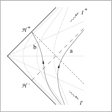
FIG. 3.: Kruskal diagram of the $r>2M$ region of Schwarzschild spacetime. This figure can be regarded as a “partial decompactification” of Fig. 2, wherein ${\cal I}^{\pm}$ are “sent to infinity” and lines $r=\mbox{const}$ are “straightened up” for large values of $r$.

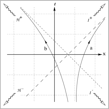
FIG. 4.: The $r>2M$ region of Schwarzschild spacetime in $(t,x)$ coordinates. This is how a $\theta=\mbox{const}$, $\varphi=\mbox{const}$ section of Schwarzschild spacetime appears when the optical metric $\tilde{g}_{ab}$ is used. The worldlines $r=\mbox{const}$ of the privileged observers have been completely straightened, and the horizons ${\cal H}^{\pm}$ have been “sent to infinity.” Notice that the observers a and b appear accelerated in this diagram.

To define “natural” observers inside the star is not so easy. In general, the metric in the internal region is not conformally static, and one cannot thus apply the construction based on the timelike conformal Killing vector field, outlined at the beginning of Sec. I. However, even when such a field exists it does not necessarily produce a satisfactory family of internal observers. This point can be clarified by considering again the example of a collapsing shell of matter. Inside the shell the spacetime is flat, by Birkhoff’s theorem; therefore, it would seem obvious to choose inertial observers at fixed distances with respect to the centre of the shell, in order to define a “rest frame.” But such observers are not the natural continuation inside the shell of the Schwarzschild static ones, defined outside. This can be seen by noticing that the horizon ${\cal H}^{+}$ is infinitely ahead in the future for the Schwarzschild observers, but not for those at rest with respect to the centre of the shell. Similarly, the Schwarzschild observers “crowd” near ${\cal H}^{+}$, unlike the internal ones (see Fig. 1). Thus, using the Schwarzschild and the inertial frames would lead to ill-behaved optical metric $\tilde{h}_{ab}$ and potential $\Phi$.

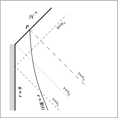
FIG. 5.: Light rays in a Kruskal diagram for spherically symmetric collapse. The outgoing ray $u=u_{0}$ is generated by the incoming one, $v=v_{0}$, after it has crossed the centre of the star. It appears reflected because the diagram is in polar coordinates.

Before constructing explicitly an extension of the Schwarzschild frame that does not suffer from these problems, let us present a graphical discussion of some of its properties. Basically, we are looking for a continuation of the coordinates $t$ and $x$ inside matter, such that ${\rm d}t/{\rm d}x=\pm 1$ for light signals and fundamental observers are located at $x=\mbox{const}$. In a $(t,x)$ diagram, the surface of the star is represented by a line like b in Fig. 4, so that we have still only to establish how the centre $r=0$ looks like. To this end, it is convenient to consider the Kruskal diagram in Fig. 5, which shows three incoming radial light rays (or spherical wavefronts). The ray at $v=v_{0}$ simply passes through the centre of the star and is then converted into an outgoing signal, $u=u_{0}$. The ray $v=v_{\scriptscriptstyle H}$ reaches $r=0$ just on the horizon and then turns into a null generator of ${\cal H}^{+}$. For $v>v_{\scriptscriptstyle H}$, all incoming signals enter the black hole region; in particular, the ray $v=v_{\scriptscriptstyle P}$ does so exactly when the surface of the star crosses the horizon (event $P$ in Fig. 5). Since light signals are still represented by straight lines at $\pm 45^{\circ}$ in the $(t,x)$ diagram, and $v_{0}$, $v_{\scriptscriptstyle H}$, $v_{\scriptscriptstyle P}$ all have finite values, it follows that the centre $r=0$ must correspond to a line that becomes asymptotically parallel to the one representing the surface of the star, as shown in Fig. 6. Since fundamental observers are represented by vertical lines $x=\mbox{const}$ in the $(t,x)$ plane, it is easy to see that their qualitative behaviour in a Kruskal diagram is the one shown in Fig. 7. Their worldlines now accumulate along the whole ${\cal H}^{+}$ and match regularly across the surface of the star. These conditions guarantee that when the metric $\tilde{g}_{ab}$ is used, ${\cal H}^{+}$ becomes a regular portion of the future asymptotic null infinity.

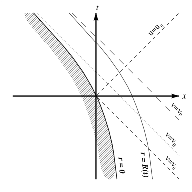
FIG. 6.: Collapse in $(t,x)$ coordinates. Both the surface and the centre of the star appear accelerated, and their worldlines are asymptotically parallel to each other. The radius of the star in the optical geometry approaches the value $v_{\scriptscriptstyle P}-v_{\scriptscriptstyle H}$ as $t\to+\infty$. Only the part of the $(t,x)$ plane above the curve $r=0$ is physically meaningful.

FIG. 7.: Regular extension of the Schwarzschild frame.

Let us now proceed to construct $n^{a}$ analytically. It is convenient to introduce new coordinates $(\tau,\xi)$ in the internal region $r<R(t)$, such that

$$-\alpha(t,r){\rm d}t^{2}+\beta(t,r){\rm d}r^{2}=\gamma(\tau,\xi)\left(-{\rm d}\tau^{2}+{\rm d}\xi^{2}\right)\;,$$ (5)

with $\gamma$ a positive function. (Such coordinates always exist, because all two-dimensional spacetimes are conformally flat.) Of course, $t$ and $r$ become now functions $t(\tau,\xi)$ and $r(\tau,\xi)$ of the new coordinates. Thus, the internal metric reads

$$g=\gamma(\tau,\xi)\left(-{\rm d}\tau^{2}+{\rm d}\xi^{2}\right)+r(\tau,\xi)^{2}\left({\rm d}\theta^{2}+\sin^{2}\theta\,{\rm d}\varphi^{2}\right)\;.$$ (6)

Since both $t$ and $\tau$ are timelike coordinates, the history of a point with $\theta=\mbox{const}$, $\varphi=\mbox{const}$ on the surface of the star consists of a sequence of events ordered in $\tau$. Therefore, in terms of the internal coordinates, the equation of the surface can be written as $\xi=\Xi(\tau)$, obtained by solving the equation $r(\tau,\xi)=R(t(\tau,\xi))$ with respect to $\xi$.

The spacetime metric must be continuous across the surface of the star. Thus, the external metric (3) and the internal one, given by (6), must agree in the evaluation of the spacetime interval between two events that occur on the star’s surface. Let us consider two such events, labeled, in the internal coordinates, by $(t,R(t),\theta,\varphi)$ and $(t+\delta t,R(t+\delta t),\theta,\varphi)\approx(t+\delta t,R(t)+R^{\prime}(t)\delta t,\theta,\varphi)$, where a prime denotes the derivative of a function with respect to its argument. Similarly, in external coordinates we have, for the same events, $(\tau,\Xi(\tau),\theta,\varphi)$ and $(\tau+\delta\tau,\Xi(\tau+\delta\tau),\theta,\varphi)\approx(\tau+\delta\tau,\Xi(\tau)+\Xi^{\prime}(\tau)\delta\tau,\theta,\varphi)$. Replacing in Eqs. (3) and (6), and equating the outcomes by continuity, we obtain a differential relation between $t$ and $\tau$ at the surface of the star,

$$\gamma(\tau,\Xi(\tau)) \left[1-\Xi^{\prime}(\tau)^{2}\right]{\rm d}\tau^{2}$$ (8)

$$=\left[C(R(t))-R^{\prime}(t)^{2}/C(R(t))\right]{\rm d}t^{2}\;.$$

Integrating Eq. (8) gives a relationship $\tau=f(t)$ between the values of $t$ and $\tau$ at the surface.

The form (6) of the internal metric is convenient because it allows one to readily define null coordinates $(U,V)$,

$$U=\tau-\xi+U_{0}\;,$$ (9)

$$V=\tau+\xi+V_{0}\;,$$ (10)

where $U_{0}$ and $V_{0}$ are arbitrary constants. The coordinates $U$ and $V$ have the usual physical meaning: The locus $U=\mbox{const}$ in spacetime is the history of an outgoing spherical wavefront of light, while $V=\mbox{const}$ represents an incoming one. If we introduce null coordinates $(u,v)$ in the outside region as

$$u=t-x\;,$$ (11)

$$v=t+x\;,$$ (12)

we have that an outgoing spherical wavefront is described, inside the star, by the equation $U=\mbox{const}$ and, outside the star, by $u=\mbox{const}$. Therefore, one can establish a one-to-one correspondence $U(u)$ between the values of $U$ and $u$, defining $U(u)$ as the internal $U$-label of the wavefront which, outside, is labeled by $u$. Similarly, one can define a function $V(v)$. The explicit form of $U(u)$ can be obtained by solving with respect to $t$ the equation

$$t-x(R(t))=u$$ (13)

and then substituting the result into

$$U=f(t)-\Xi(f(t))+U_{0}\;.$$ (14)

Analogously, $V(v)$ is obtained by replacing the solution of

$$t+x(R(t))=v$$ (15)

into

$$V=f(t)+\Xi(f(t))+V_{0}\;.$$ (16)

The functions $U(u)$ and $V(v)$ can be used to extend the coordinates $(u,v)$, hence $(t,x)$, also inside the star. It is sufficient to invert them, getting $u$ and $v$ as functions of $U$ and $V$, respectively, and then define $t$ and $x$ as

$$t:={1\over 2}\,\left(v(V)+u(U)\right)\;,$$ (17)

$$x:={1\over 2}\,\left(v(V)-u(U)\right)\;.$$ (18)

In terms of $t$ and $x$, the internal metric (6) takes the form

$$g=\gamma U^{\prime}V^{\prime}\left(-{\rm d}t^{2}+{\rm d}x^{2}\right)+r^{2}\left({\rm d}\theta^{2}+\sin^{2}\theta\,{\rm d}\varphi^{2}\right)\;,$$ (19)

where $U^{\prime}:={\rm d}U/{\rm d}u$, $V^{\prime}:={\rm d}V/{\rm d}v$, and all the functions are implicitly supposed to be expressed in terms of $t$ and $x$. Now we choose

$$\Phi={1\over 2}\,\ln\left(\gamma U^{\prime}V^{\prime}\right)\;,$$ (20)

so that the internal optical metric reads

$$\tilde{g}=-{\rm d}t^{2}+{\rm d}x^{2}+{r^{2}\over\gamma U^{\prime}V^{\prime}}\,\left({\rm d}\theta^{2}+\sin^{2}\theta\,{\rm d}\varphi^{2}\right)\;.$$ (21)

In $(t,r)$ coordinates, the optical frame $n^{a}$ has components $n^{\mu}=\left(\gamma U^{\prime}V^{\prime}\right)^{-1/2}\delta^{\mu}_{t}$, i.e., in $(\tau,\xi)$ coordinates,

$$n^{\mu}={1\over 2(\gamma U^{\prime}V^{\prime})^{1/2}}\left[\left(V^{\prime}+U^{\prime}\right)\delta^{\mu}_{\tau}+\left(V^{\prime}-U^{\prime}\right)\delta^{\mu}_{\xi}\right]\;.$$ (22)

This vector field is a satisfactory extension inside the star of the static Schwarzschild frame, and it is not difficult to check that, although the metric (19) is not conformally static, Eq. (1) is still satisfied. Thus, we can continue to interpret $\Phi$ as the gravitational potential.

The factor $U^{\prime}V^{\prime}$ can be computed as follows. Let us consider two outgoing light rays, corresponding to the values $U$ and $U+\delta U$, $u$ and $u+\delta u$ of the coordinates, with $\delta U$ and $\delta u$ very small. Equations (13) and (14) give us the coordinate times $t$ and $t+\delta t$ at which these rays cross the surface of the star, expressed as functions of $u$, $u+\delta u$, $U$, and $U+\delta U$. This allows us to find the coefficients that link $\delta u$ and $\delta U$ to $\delta t$; eliminating $\delta t$ and taking the limit, we get

$${{\rm d}U\over{\rm d}u}={1-\Xi^{\prime}(f(t(u)))\over 1-R^{\prime}(t(u))/C(R(t(u)))}\,f^{\prime}(t(u))\;,$$ (23)

where the function $t(u)$ is implicitly defined by Eq. (13). Similarly, one obtains from Eqs. (15) and (16), considering two incoming light rays,

$${{\rm d}V\over{\rm d}v}={1+\Xi^{\prime}(f(t(v)))\over 1+R^{\prime}(t(v))/C(R(t(v)))}\,f^{\prime}(t(v))\;,$$ (24)

where now $t(v)$ is given by Eq. (15). Using Eq. (8) we get at the end:

$$U^{\prime}(u)V^{\prime}(v) =\left[{1-\Xi^{\prime}(f(t(u)))\over 1+\Xi^{\prime}(f(t(u)))}\,{1+\Xi^{\prime}(f(t(v)))\over 1-\Xi^{\prime}(f(t(v)))}\right.$$ (29)

$$\times{1+R^{\prime}(t(u))/C(R(t(u)))\over 1-R^{\prime}(t(u))/C(R(t(u)))}$$

$$\times{1-R^{\prime}(t(v))/C(R(t(v)))\over 1+R^{\prime}(t(v))/C(R(t(v)))}$$

$$\times{C(R(t(u)))\over\gamma(f(t(u)),\Xi(f(t(u))))}$$

$$\left.\times{C(R(t(v)))\over\gamma(f(t(v)),\Xi(f(t(v))))}\right]^{1/2}\;.$$

III Asymptotic behaviour

Equations (20)–(29) give a complete characterization of the optical geometry inside a collapsing spherically symmetric star. Of course, since they require an explicit knowledge of the functions $R(t)$, $\Xi(\tau)$, $f(t)$, and $\gamma(\tau,\xi)$, one can use them only within a specific model of collapse — and even in that case their integration will usually require numerical methods. It is therefore remarkable that, at late times (i.e., for $t,u\to+\infty$), one could establish analytically some features that are universal, in the sense that they do not depend on the details of the model.

In the limit $u\to+\infty$, it is easy to circumvent the nasty expression on the right hand side of Eq. (23) by noticing that, although the relationship between the functions $U$ and $u$ is singular on ${\cal H}^{+}$, $U$ is regularly connected to the Kruskal retarded null coordinate [4]

$${\cal U}=-\exp(-u/4M)$$ (30)

for all values of $\cal U$; this follows from the fact that both $(U,V)$ and the Kruskal coordinates are regular at the surface of the star. Then, two outgoing light rays, labeled by $U$ and $U+\delta U$ inside the star, are labeled by $\cal U$ and ${\cal U}+\delta{\cal U}$ outside, with $\delta U=a({\cal U})\delta{\cal U}$, where $a$ is a regular positive function that depends on the details of collapse (i.e., $R$, $R^{\prime}$, $\Xi$, and $\Xi^{\prime}$) at the moment when the light rays cross the surface of the star. For rays near the horizon, i.e., in the limit $u\to+\infty$, one has ${\cal U}\approx 0$ and thus $\delta U\approx a(0)\delta{\cal U}$, which gives the desired asymptotic relation [16]

$${{\rm d}U\over{\rm d}u}\sim{a(0)\over 4M}\exp(-u/4M)\;.$$ (31)

(Hereafter, we use the notation $f_{1}\sim f_{2}$ to express the fact that two functions have the same asymptotic expression in some limit, i.e., $\lim f_{1}/f_{2}=1$.) The constant positive factor $a(0)$ is all that remains of the details of collapse in the limit $u\to+\infty$.

The situation is rather different as far as ${\rm d}V/{\rm d}v$ is concerned. Of course, considering two incoming light rays labeled by $V$ and $V+\delta V$ inside the star, and by $\cal V$ and ${\cal V}+\delta{\cal V}$ outside, where

$${\cal V}=\exp(v/4M)$$ (32)

is the Kruskal advanced null coordinate, one can still claim that $\delta V=b({\cal V})\delta{\cal V}$, where $b$ is a regular positive function depending on the dynamics of the star’s surface when it is crossed by the light rays. However, since the interior of the star at ${\cal H}^{+}$ corresponds to an entire range of values for $V$ and $v$ (the interval $[v_{\scriptscriptstyle H},v_{\scriptscriptstyle P}]$ in Fig. 5), the function ${\rm d}V/{\rm d}v$, although regular everywhere, has not a universal dependence on $v$.

The asymptotic form (31) of $U^{\prime}(u)$ and the regular dependence of $V^{\prime}$ on $v$ are nevertheless sufficient in order to establish the main properties of optical geometry during the late stages of collapse. Since $\gamma$, $U^{\prime}$, and $V^{\prime}$ are regular positive functions, the product $\gamma U^{\prime}V^{\prime}$ can simply be written as

$$\gamma U^{\prime}V^{\prime}\sim F(v)\exp(-u/4M)\;,$$ (33)

where $F(v)$ is a non-vanishing positive function which depends on the details of collapse. Of course, outside the star, $U\equiv{\cal U}$, $V\equiv{\cal V}$, and $\gamma=(32M^{3}/r)\exp(-r/2M)$, so $\gamma U^{\prime}V^{\prime}=1-2M/r$ and $F(v)\sim\exp(-1+v/4M)$.

From Eq. (22) it is evident that, since $U^{\prime}\to 0$ when $u\to+\infty$, the optical frame behaves like the one in Fig. 7, because the components $n^{\tau}$ and $n^{\xi}$ tend to become equal near ${\cal H}^{+}$. The optical metric (21) and the potential $\Phi$ have the following asymptotic forms:

$$\tilde{g}\sim-{\rm d}t^{2}+{\rm d}x^{2}+{4M^{2}\,{\rm e}^{(t-x)/4M}\over F(t+x)}\left({\rm d}\theta^{2}+\sin^{2}\theta\,{\rm d}\varphi^{2}\right)\;;$$ (34)

$$\Phi\sim{x-t\over 8M}+{1\over 2}\,\ln F(t+x)\;.$$ (35)

Using Eq. (1), one can easily compute the acceleration of the fundamental observers. The only nonvanishing component is

$$n^{a}\nabla\!_{a}n_{x}={\partial\Phi\over\partial x}={1\over 8M}+{F^{\prime}(t+x)\over 2F(t+x)}\;,$$ (36)

which gives, up to the sign, the value of the “gravitational field” at late times. It is interesting to notice that, outside the star, $n^{a}\nabla\!_{a}n_{x}=1/4M$, which coincides with the surface gravity of the black hole (see Appendix B for a general proof). On the other hand, inside the star, the term $F^{\prime}/2F$ gives a correction to the surface gravity that varies from place to place on the horizon and depends on the model of collapse.

Let us now consider a timelike hypersurface with equation $\xi=F(\tau)$, such that near ${\cal H}^{+}$ one can write $\xi\sim\nu\tau+\mbox{const}$, where $\nu$ is a constant (from the expression (6) of the metric, it follows that $-1<\nu<1$). This is the case, for example, of the centre of the star, $\xi\equiv 0$, or of the star’s surface, for which we have $\nu={\rm d}\Xi/{\rm d}\tau$ evaluated at the horizon. Equations (9) and (10) give then $(1+\nu){\rm d}U\approx(1-\nu){\rm d}V$. Near ${\cal H}^{+}$, the coordinate $v$ is approximately constant on the submanifold identified by $\xi=F(\tau)$ (for example, in the cases of the centre and of the surface of the star, it is equal to $v_{\scriptscriptstyle H}$ and $v_{\scriptscriptstyle P}$, in the notations of Fig. 5), and this relation can be rewritten as

$${\rm d}v\sim A\exp(-u/4M){\rm d}u\;,$$ (37)

where $A$ is a cumulative positive constant and we have used Eq. (31). Integrating and using Eq. (12), we get

$$t+x\sim\bar{v}-K\exp(-u/4M)\;,$$ (38)

where $K:=4MA>0$ and the integration constant $\bar{v}$ is the advanced time at which the surface $\xi=F(\tau)$ crosses ${\cal H}^{+}$. Equation (38) can be rewritten using Eq. (11) as

$$x\sim-t+\bar{v}-K\exp(-t/2M)$$ (39)

(see also Ref. [14], p. 869, and Ref. [17]). This equation expresses the asymptotic behaviour, in $(t,x)$ coordinates, of any worldline that crosses ${\cal H}^{+}$. Of course, it is valid both inside and outside the star.

IV Example: The Oppenheimer-Snyder model

In order to apply the general techniques developed so far to a specific case, let us consider the simplest model of a collapsing star, in which matter is a ball of dust with uniform density [18]. In this case, the internal solution is part of a spatially closed Friedman spacetime (see Ref. [14], pp. 851–856), so we have $\gamma(\tau,\xi)=a(\tau)^{2}/a_{0}^{2}$ and

$$r(\tau,\xi)=a(\tau)\sin(\xi/a_{0})\;,$$ (40)

where $0\leq\tau<\pi a_{0}$ ($\tau=0$ corresponds to the beginning of collapse), $a_{0}$ is a constant, $0\leq\xi\leq\Xi_{0}$, with $\Xi_{0}<\pi a_{0}/2$ corresponding to the surface of the star, and

$$a(\tau)=a_{0}\cos^{2}(\tau/2a_{0})\;.$$ (41)

It is convenient to introduce the dimensionless variable $\sigma:=\tau/2a_{0}$. Then, the function $R(t)$ is defined implicitly by the two equations

$$R=R_{i}\cos^{2}\sigma$$ (42)

and

$$t = 2M\ln\left[{\left({\displaystyle{R_{i}\over 2M}}-1\right)^{1/2}+\tan\sigma\over\left({\displaystyle{R_{i}\over 2M}}-1\right)^{1/2}-\tan\sigma}\right]$$ (43)

$$+ 4M\left({R_{i}\over 2M}-1\right)^{1/2}\left[\sigma+{R_{i}\over 4M}\left(\sigma+\sin\sigma\cos\sigma\right)\right]\;,$$ (44)

where $R_{i}=a_{0}\sin(\Xi_{0}/a_{0})$ is the radius of the star at the beginning of collapse. Note that for $\sigma=\sigma^{\ast}:=\arccos\sqrt{2M/R_{i}}$, which corresponds to the event horizon, one has $t=+\infty$, as it should be.

In this model one has $\Xi(\tau)=\Xi_{0}=\mbox{const}$. The functions $U(u)$ and $V(v)$ can, in principle, be obtained by the systems

$$\left.\matrix{u&=&t-X\hfill\cr U&=&\tau-\Xi_{0}+U_{0}\cr}\right\}$$ (46)

and

$$\left.\matrix{v&=&t+X\hfill\cr V&=&\tau+\Xi_{0}+V_{0}\cr}\right\}\;,$$ (47)

respectively, where $X=R+2M\ln\left(R/2M-1\right)$ and both $R$ and $t$ are expressed in terms of $\tau$, according to Eqs. (42) and (LABEL:T). From now on, we shall exploit the freedom in the constants $U_{0}$ and $V_{0}$, choosing $U_{0}=-V_{0}=\Xi_{0}$, so that $U=V=\tau$ at the surface of the star. In practice, Eq. (LABEL:T) is a transcendental one for $\tau$ and cannot be inverted. However, we can easily find the inverse functions $u(U)$ and $v(V)$. Consider an outgoing spherical wavefront of light, characterized by $U=\bar{U}=\mbox{const}$ and $u=\bar{u}=\mbox{const}$, respectively inside and outside the star. In particular, we must have $\bar{u}=t(\bar{\tau})-X(\bar{\tau})$, where $\bar{\tau}$ is the value of $\tau$ at the moment when the wavefront crosses the surface of the star. But from Eq. (46) we have also $\bar{U}=\bar{\tau}$, so Eqs. (42) and (LABEL:T) allow us to conclude that, inside the star, the relationship between $U$ and $u$ is

$$u(U) = t(\tau=U)-X(\tau=U)$$ (48)

$$= -4M\ln\left({R_{i}\over 2M}\cos^{2}\sigma_{\scriptscriptstyle U}-1\right)$$ (49)

$$+ 4M\ln\left[\left({R_{i}\over 2M}-1\right)^{1/2}+\tan\sigma_{\scriptscriptstyle U}\right]-R_{i}\cos^{2}\sigma_{\scriptscriptstyle U}$$ (50)

$$+ 2M\ln\cos^{2}\sigma_{\scriptscriptstyle U}+4M\left({R_{i}\over 2M}-1\right)^{1/2}\sigma_{\scriptscriptstyle U}$$ (51)

$$+ R_{i}\left({R_{i}\over 2M}-1\right)^{1/2}\left(\sigma_{\scriptscriptstyle U}+\sin\sigma_{\scriptscriptstyle U}\cos\sigma_{\scriptscriptstyle U}\right)\;,$$ (52)

with $\sigma_{\scriptscriptstyle U}=U/2a_{0}$. Analogously, we find

$$v(V) = t(\tau=V)+X(\tau=V)$$ (53)

$$= 4M\ln\left[\left({R_{i}\over 2M}-1\right)^{1/2}+\tan\sigma_{\scriptscriptstyle V}\right]+R_{i}\cos^{2}\sigma_{\scriptscriptstyle V}$$ (54)

$$+ 2M\ln\cos^{2}\sigma_{\scriptscriptstyle V}+4M\left({R_{i}\over 2M}-1\right)^{1/2}\sigma_{\scriptscriptstyle V}$$ (55)

$$+ R_{i}\left({R_{i}\over 2M}-1\right)^{1/2}\left(\sigma_{\scriptscriptstyle V}+\sin\sigma_{\scriptscriptstyle V}\cos\sigma_{\scriptscriptstyle V}\right)\;,$$ (56)

where $\sigma_{\scriptscriptstyle V}=V/2a_{0}$. Substituting Eqs. (52) and (56) into Eqs. (17) and (18), we can express $t$ and $x$ inside the star as functions of $U$ and $V$.

Along the worldlines of the observers belonging to the optical frame one has $x=\mbox{const}$, i.e., ${\rm d}u/{\rm d}v=1$. Writing Eqs. (52) and (56) in differential form,

$${\rm d}u={R_{i}^{2}\cos^{4}\sigma_{\scriptscriptstyle U}\over 2a_{0}M}\cdot{{\displaystyle\left({R_{i}\over 2M}-1\right)^{1/2}}+\tan\sigma_{\scriptscriptstyle U}\over{\displaystyle{R_{i}\over 2M}}\cos^{2}\sigma_{\scriptscriptstyle U}-1}\,{\rm d}U\;,$$ (57)

$${\rm d}v={R_{i}^{2}\cos^{4}\sigma_{\scriptscriptstyle V}\over 2a_{0}M}\cdot{{\displaystyle\left({R_{i}\over 2M}-1\right)^{1/2}}-\tan\sigma_{\scriptscriptstyle V}\over{\displaystyle{R_{i}\over 2M}\cos^{2}\sigma_{\scriptscriptstyle V}-1}}\,{\rm d}V\;,$$ (58)

we find the slope of these worldlines in $(U,V)$ coordinates:

$${{\rm d}U\over{\rm d}V} ={\left(\cos^{2}\sigma_{\scriptscriptstyle U}-{\displaystyle{2M\over R_{i}}}\right)\cos^{4}\sigma_{\scriptscriptstyle V}\over\left(\cos^{2}\sigma_{\scriptscriptstyle V}-{\displaystyle{2M\over R_{i}}}\right)\cos^{4}\sigma_{\scriptscriptstyle U}}$$ (60)

$$\times{\left({\displaystyle{R_{i}\over 2M}}-1\right)^{1/2}-\tan\sigma_{\scriptscriptstyle V}\over\left({\displaystyle{R_{i}\over 2M}}-1\right)^{1/2}+\tan\sigma_{\scriptscriptstyle U}}\;.$$

This equation can be integrated numerically for suitable values of $M$ and $R_{i}$, and produces diagrams that agree with our qualitative sketch of Fig. 7.

The function $u(U)$ assumes a particularly simple asymptotic form near the event horizon, in agreement with the general analysis in Sec. III. The surface of the star crosses the horizon when $R=2M$, i.e., at a time $\tau=\tau^{\ast}$ such that $\cos^{2}\sigma^{\ast}=2M/R_{i}$. Since the horizon is a null hypersurface with $U=U^{\ast}=\mbox{const}$, we have also that $\cos^{2}\sigma^{\ast}_{\scriptscriptstyle U}=2M/R_{i}$. Then, for $U\to U^{\ast}$ the first term on the right hand side of Eq. (52) dominates and one can write, asymptotically,

$$u(U)\sim-4M\ln\left(\sigma^{\ast}_{\scriptscriptstyle U}-\sigma_{\scriptscriptstyle U}\right)\;.$$ (61)

Consistently, one finds from Eq. (57) that ${\rm d}u/{\rm d}U\sim-4M/(U-U^{\ast})$; in fact, this relationship is not restricted to the present model and holds for a generic collapse, as it follows from Eq. (31). Since $v(V)$ remains finite, we have also

$$t(U,V)\sim-2M\ln\left(\sigma^{\ast}_{\scriptscriptstyle U}-\sigma_{\scriptscriptstyle U}\right)$$ (62)

and

$$x(U,V)\sim 2M\ln\left(\sigma^{\ast}_{\scriptscriptstyle U}-\sigma_{\scriptscriptstyle U}\right)\;.$$ (63)

Notice that $t\to+\infty$ and $x\to-\infty$ for $U\to U^{\ast}$. The worldlines of the observers belonging to the optical frame, $x=\mbox{const}$, tend to lie along the event horizon, as one can also see from Eq. (60), which implies ${\rm d}U/{\rm d}V\to 0$ as $U\to U^{\ast}$. All these features are very satisfactory from the point of view of a smooth extension of the Schwarzschild rest frame inside the star, and are in full agreement with the general results obtained in Sec. III.

V Hawking effect

We now want to figure out how collapse looks like in the optical geometry. For this purpose it is convenient to consider the embedding diagrams of an equatorial plane at different values of $t$ (see Ref. [19] for a general discussion of embedding diagrams). When $R>3M$, there are no qualitative differences with respect to the conventional description (see Fig. 8). However, as $R$ becomes smaller than $3M$, a “throat” develops in the external space, in correspondence with $r=3M$, while the surface of the star expands progressively (Figs. 9 and 10), escaping to $x\to-\infty$ with the asymptotic law (39). Thus, “collapse” actually corresponds, in the optical geometry, to a sort of expansion into a space that is created by the process itself. This picture is less absurd than it may seem, if one remembers the operational meaning of optical distance outlined in Sec. I. Consider an observer standing at a large value of $r$, who sends light signals on a mirror that has been previously placed at the centre of the star, and then defines his distance from the centre simply in terms of the lapse of Killing time $t$ taken by the round trip. Since the time delay becomes progressively larger, he will deduce that a collapsing star recedes from him at an increasing speed. Because of spherical symmetry, the only geometrical picture consistent with this description is the one of Figs. 8–10, where the star expands into a “lower space” that is created in the course of collapse.

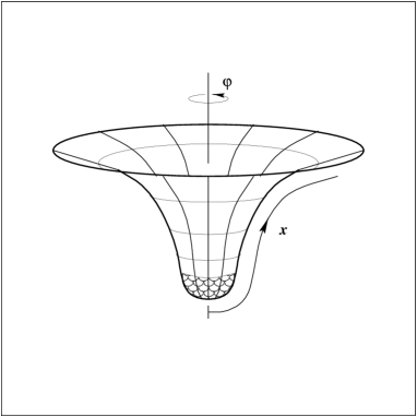
FIG. 8.: Embedding diagram of the $\theta=\pi/2$ section of optical space at an early stage of collapse. Points in the shadowed area are located inside the star.

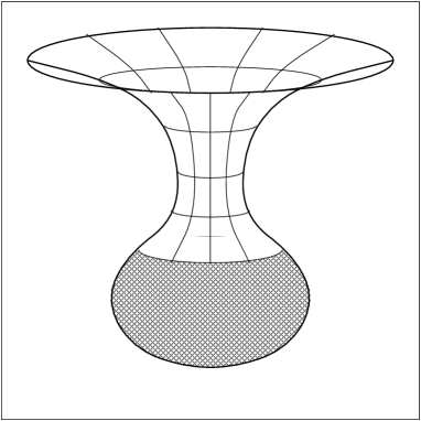
FIG. 9.: The shape of the $\theta=\pi/2$ section of optical space when $3M>R(t)>9M/4$.

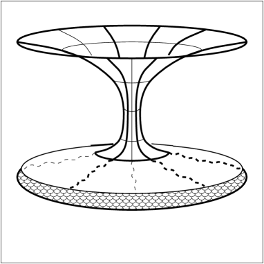
FIG. 10.: When $R(t)<9M/4$, no faithful embedding is possible in the three-dimensional Euclidean space. The star escapes to $x\to-\infty$ at an increasing speed. The optical radial distance between the centre $r=0$ and the surface $r=R(t)$ tends to the finite value $v_{\scriptscriptstyle P}-v_{\scriptscriptstyle H}$ when $t\to+\infty$, while the area of the surface increases without bound.

If a quantum field is present, this dynamical process disturbs its modes analogously to what happens when there is a moving boundary. In fact, in the two-dimensional section shown in Fig. 6, the situation is exactly the same as if there were a moving boundary, that accelerates asymptotically towards the speed of light, with the law (39). In Minkowski spacetime, this is known to lead, at late times $t$, to a thermal flux of radiation with temperature $(8\pi M)^{-1}$ [20] (see also Ref. [16], pp. 102–109 and 229). Given the identity between the $(t,x)$ part of the line element of $\tilde{g}_{ab}$ with the one of a two-dimensional Minkowski spacetime, one expects therefore that even in the late stages of collapse there must be a flux of radiation at temperature $T_{\scriptscriptstyle H}=(8\pi M)^{-1}$. This is precisely the quantum emission found by Hawking [13, 16, 20], whose existence follows therefore in a natural way from the picture of collapse based on the optical geometry. It is remarkable that, although the moving boundary analogy has often been used in the literature [20], optical geometry gives a very simple physical explanation of why it works: Essentially, because gravitational collapse is a particular case of a moving boundary.

Actually, the analogy with a moving boundary in Minkowski spacetime fails to hold exactly when the angular dimensions are taken into account, because the field propagates on a non-Euclidean geometry. However, this has the only effect of distorting the spectrum of the emitted radiation, according to the way waves are scattered by the curvature of space. Such a correction is well-known in the theory of the Hawking effect [13, 16].

In this picture the event horizon does not play any role in deriving Hawking’s radiation. In this respect, it is worth reminding that in the optical geometry the horizon is very much alike to a portion of the asymptotic null infinity. To claim that it has anything to do with the thermal flux from black holes would be exactly analogous to saying that the future null infinity is relevant for the radiation produced by a moving boundary in Minkowski spacetime. Thus, explanations of the effect based on quantum tunneling mechanisms appear rather implausible from the perspective of optical geometry.

A similar situation occurs for black hole entropy. In the optical geometry, the celebrated relation $S=A/4$ has no direct meaning, because the horizon has an infinite area according to the metric $\tilde{h}$. Indeed, the horizon is located at $x\to-\infty$ in the optical space. If some notion of entropy can be introduced, it can therefore be associated only with the region $r>2M$. One possibility is to attribute the entropy entirely to the Hawking radiation, in the following way. Let us consider Fig. 10 again, where the space around a collapsing star at sufficiently late times is visualized as made of a vast “lower” region connected to the usual “upper” one through a mouth at $r=3M$. To observers living at large values of $r$, the $r=3M$ surface looks like the boundary of a three-dimensional cavity containing thermal black body radiation at the temperature $T_{\scriptscriptstyle H}$. (One may even consider the $r<3M$ region as analogous to a Kirchhoff cavity in ordinary thermodynamics.) Whenever a small amount of energy $\Delta E$ escapes to infinity as Hawking’s radiation, or is added to the collapsing star in the form of accreted matter, the total entropy of the radiation contained in the cavity is modified by the amount $\Delta S=\Delta E/T_{\scriptscriptstyle H}$. Since $\Delta E$ coincides with the change in the mass, as measured from infinity, we recover the Beckenstein-Hawking expression $S=4\pi M^{2}$ [13, 20, 21] in its differential form. Thus, optical geometry suggests that one should regard the so-called black hole entropy as being actually associated with the Hawking radiation surrounding the collapsing star. This interpretation contrasts with a viewpoint often expressed, according to which $S$ is a property of spacetime, and is similar to others that attribute entropy to a “thermal atmosphere” of the black hole [22].

Until now, we have assumed that the quantum field is a test one, i.e., that it does not affect the background spacetime. Clearly, this approximation becomes invalid at late times, when the amount of energy carried away by the Hawking radiation that leaks through the neck at $r=3M$ becomes a non-negligible fraction of the mass $M$ of the star. Let us then sketch qualitatively how back-reaction modifies the picture of collapse suggested by the optical geometry. Roughly, the main effect of Hawking’s emission is to decrease the value of $M$. This has essentially three consequences on the diagram of Fig. 10: First, it decreases the size of the mouth at $r=3M$; second, it increases the curvature of the optical space at the mouth and in the lower region; third, it increases the value of the Hawking temperature $T_{\scriptscriptstyle H}$. Thus, as the process goes on and more radiation is able to escape to $r\to+\infty$, the geometry in the region $r>3M$ of space becomes closer and closer to the Euclidean one, while the throat at $r=3M$ shrinks down, becoming progressively sharper. The region $r<3M$ has larger and larger negative curvature and contains, at large negative values of $x$, matter that escapes to $x\to-\infty$ with increasing acceleration.

Although this description is purely qualitative and is not based on an explicitly constructed model, it gives us important clues about the issue of the final state of a collapsing star, when Hawking’s radiation is taken into account. First of all, it implies that the black hole, in the strict sense of the region beyond the future event horizon ${\cal H}^{+}$, does not form. This is evident in the optical geometry point of view, where ${\cal H}^{+}$ corresponds to $x\to-\infty$ and $t\to+\infty$. In the usual language, one would say that radiation makes the value of $M$ decrease, which in turn makes the horizon shrink, and eventually reduce to a point before the star could cross it. Thus, the very existence of the Hawking effect would prevent the formation of black holes by collapse.

If this is the case, what are then we left with in the limit $t\to+\infty$? A straightforward extrapolation of the process that we have just described suggests that, for $M\to 0$, the throat at $r=3M$ pinches off, leaving two spaces — one Euclidean, the other with infinite negative curvature — with just one point in common. This is clearly a degenerate, and highly implausible, situation; one would rather think that the process stops when the throat reaches a critical size (perhaps at the Planckian scale), because of as yet unknown physical processes. Such a situation corresponds to the hypothesis of remnants in the common description [24, 25].

Remnants have originally been introduced as a possible resolution of the information paradox [25, 26]. However, the viability of this hypothesis has sometimes been questioned, because the small scale and mass of remnants would allow them to store very little information [27]. Roughly, the argument is the following. A physical system with size $l$, total energy $E$, and Hamiltonian bounded from below has a number of states of the order of $El$; thus, it can contain a maximum information which is also of order $El$. The status of this claim is rather controversial [28]. However, even assuming that there is indeed such an information bound, it would hardly represent a difficulty in optical geometry, where the “remnant” is actually an enormously vast region, because ordinary distances are rescaled by a huge factor. Even if $l$ should represent the size of the remnant as seen from the exterior, as suggested by Bekenstein [27], the bound would still be circumvented thanks to the existence, in the lower space, of an enormous supply of negative energy associated with the field $\Phi$.

VI Conclusions and outlooks

We have constructed the optical geometry for a spherically symmetric collapsing body. The procedure adopted is a simple extension of the technique used when defining optical distance operationally in a static spacetime. Essentially, for any spacetime event $P$, one considers the in- and out-going spherical light-fronts that cross at $P$. These correspond to well-defined values of advanced and retarded time $v$ and $u$, that can be read at infinity as the affine parameters along the null generators of ${\cal I}^{-}$ and ${\cal I}^{+}$. The event $P$ is then labeled by $v$ and $u$, in addition to the angular coordinates, and can also be identified by a timelike coordinate $t:=(v+u)/2$ and a spacelike one, $x:=(v-u)/2$. The optical metric is then defined as the only one which is conformal to $g_{ab}$ — the metric of spacetime in general relativity — and which reproduces the two-dimensional Minkowskian line element on $\theta=\mbox{const}$, $\varphi=\mbox{const}$ sections. Outside the collapsing star, $g_{ab}$ has the Schwarzschild form and $x$ coincides with the Regge-Wheeler “tortoise” coordinate, thus giving the well-known optical metric of an empty, spherically symmetric spacetime. However, our construction allows one to extend the optical geometry smoothly inside the star.

Associated with the optical space are the optical frame $n^{a}$, made of the observers at $x=\mbox{const}$, and the scalar potential $\Phi$, essentially the logarithm of the conformal factor that links $g_{ab}$ and $\tilde{g}_{ab}$. These two concepts are related to each other in the following sense. The optical frame defines a notion of “rest in the gravitational field,” thus the four-acceleration $n^{b}\nabla\!_{b}n_{a}$ of the observers can be identified with the gravitational acceleration, changed of sign. Since $n^{b}\nabla\!_{b}n_{a}$ is equal to the spatial gradient of $\Phi$ in the optical frame, see Eq. (1), $\Phi$ can be thought of as a covariant generalization of the gravitational potential. This allows one to give a precise meaning to the notion of gravitational field inside a collapsing object. It must be noted that a gravitational field so defined, although analogous to the same Newtonian concept, nevertheless differs from it in some essential details. As an example, consider a collapsing spherical shell. It is obvious from Fig. 7 that $n^{b}\nabla\!_{b}n_{a}\neq 0$ everywhere, thus leading to the conclusion that the gravitational field is nonvanishing inside the shell, as well as outside. This contrasts with intuition shaped after Newton’s theory, according to which the gravitational field inside the shell should be zero. However, this difference is not surprising if one considers that $\Phi$ does not obey the Poisson equation, but a nonlinear generalization of it, as can be easily checked on replacing $g_{ab}={\rm e}^{2\Phi}\tilde{g}_{ab}$ in the trace of the Einstein equation.

Although we have focused our treatment on the case of a star collapsing in empty space, generalizations to, e.g., the collapse of electrically charged bodies are straightforward (see, e.g., Ref. [15] for a configuration with extremal charge, $Q^{2}=M^{2}$). In fact, the construction presented in Sec. II makes a heavy use of the null structure on ${\cal I}^{\mp}$ in defining the coordinates $v$ and $u$, but seems rather general otherwise. It would be important to understand whether a similar technique could be used to define optical geometry in still more general situations — for example, for non-spherically symmetric collapse.

We have seen that, in optical geometry, gravitational collapse corresponds to a very fast expansion of the star into a “lower space,” with the centre receding from the optical observers $n^{a}$ at a speed that approaches exponentially the speed of light. This process excites the modes of a quantum field, as it happens in the presence of a moving boundary, leading to the production of Hawking radiation. Thus, optical geometry provides one with a physical origin of the formal “moving mirror analogy” of the Hawking effect.

The issue of the final state of black hole evaporation is also clarified by the use of optical geometry. There are essentially two possibilities, in both of which the black hole does not form, strictly speaking. Either the evaporation process continues until one remains with flat space and a (physically unaccessible) infinitely warped “lower space” or, perhaps more likely, the process stops at some scale leaving an enormously large remnant. In both cases there is no information paradox. Of course, since the issue involves distances of the order of the Planck length, a definitive answer is beyond the limits of applicability of present-day physics. Nevertheless, it would be useful to get a more detailed insight into the evaporation process by reformulating simple models that include back-reaction (see, e.g., Ref. [31]) in the language of optical geometry.

Of course, all our conclusions apply to black holes deriving from collapse. However, it is not difficult to extend them to eternal black holes, simply studying the quantum field theory on the optical spacetime associated with the Schwarzschild solution. In this case there is no moving boundary, and the optical metric looks (as far as the $t$ and $x$ coordinates are concerned) exactly like the Minkowski one. In particular, the observers at $x=\mbox{const}$, belonging to the optical frame, correspond to the Minkowskian inertial observers. Thus, one expects that they should register no particles, provided that a condition of “no incoming radiation” is imposed for $t\to-\infty$. This is precisely what happens in the so-called Boulware (or Schwarzschild) state $|0_{\scriptscriptstyle B}\rangle$ [32]. The optical geometry viewpoint provides therefore support for regarding $|0_{\scriptscriptstyle B}\rangle$, rather than the Hartle-Hawking (or Kruskal) and the Unruh states $|0_{\scriptscriptstyle H}\rangle$ and $|0_{\scriptscriptstyle U}\rangle$ (see Ref. [16], pp. 281–282), as describing the quantum vacuum around an eternal black hole.

The Boulware state is often considered pathological because the expectation value of several physical quantities diverges at the horizon [33]. For example, for the stress-energy-momentum tensor operator of a massless scalar field $\phi$ one has, after renormalization, that $\langle 0_{\scriptscriptstyle B}|T_{ab}|0_{\scriptscriptstyle B}\rangle_{\rm ren}$ depends on $r$ as $(1-2M/r)^{-1}$ for $r\to 2M$. It is remarkable that, in the optical spacetime $({\cal M},\tilde{g}_{ab})$, such a factor is exactly canceled out, because $\phi$ is conformally transformed in $\tilde{\phi}={\rm e}^{\Phi}\phi$, and $\langle 0_{\scriptscriptstyle B}|\widetilde{T}_{ab}|0_{\scriptscriptstyle B}\rangle_{\rm ren}$ turns out to be finite everywhere, representing just the vacuum polarization due to curvature. A similar situation occurs when considering the response function $\Pi(\omega|r)$ for an ideal static detector in the Boulware state. In the spacetime $({\cal M},g_{ab})$ one has, near the horizon [33],

$$\Pi(\omega|r)\sim-{1\over 1-2M/r}{\omega\over 2\pi}\,\Theta(-\omega)\;,$$ (64)

where $\Theta$ is the step function. However, after the conformal rescaling the response is given by

$$\widetilde{\Pi}(\omega|r)\sim-{\omega\over 2\pi}\,\Theta(-\omega)\;,$$ (65)

which not only is finite, but is also the answer one would expect in a proper “vacuum.” Thus, the pathologies of the Boulware state are removed by the conformal transformation to the optical spacetime, in which $|0_{\scriptscriptstyle B}\rangle$ behaves as a satisfactory quantum vacuum.

Appendix A: Proof of Eq. (1)

¿From the definition (2) of $\Phi$ it follows that the vector field $n^{a}$ can be expressed as $n^{a}={\rm e}^{-\Phi}\eta^{a}$. Thus,

$$n^{b}\nabla\!_{b}n_{a}={\rm e}^{-2\Phi}\left(\eta^{b}\nabla\!_{b}\eta_{a}-\eta_{a}\eta^{b}\nabla\!_{b}\Phi\right)\;.$$ (A.1)

Using now the relation

$$\nabla\!_{a}\eta_{b}+\nabla\!_{b}\eta_{a}={1\over 2}\,g_{ab}\nabla\!_{c}\eta^{c}\;,$$ (A.2)

valid for any conformal Killing vector field $\eta^{a}$ (see e.g. Ref. [4], pp. 443–444), we can write

$$\eta^{b}\nabla\!_{b}\eta_{a}={\rm e}^{2\Phi}\nabla\!_{a}\Phi+{1\over 2}\,\eta_{a}\nabla\!_{b}\eta^{b}\;.$$ (A.3)

Furthermore,

$$\eta^{b}\nabla\!_{b}\Phi={\eta^{b}\eta^{c}\nabla\!_{b}\eta_{c}\over\eta_{a}\eta^{a}}={\eta^{b}\eta^{c}\nabla\!_{(b}\eta_{c)}\over\eta_{a}\eta^{a}}={1\over 4}\,\nabla\!_{b}\eta^{b}\;.$$ (A.4)

Substituting Eq. (A.4) into Eq. (A.3) and then the latter into Eq. (A.1) we obtain, after some trivial algebra, Eq. (1).

Appendix B: Physical meaning of the surface gravity in optical geometry

Here we show that, for a static black hole, the surface gravity coincides with the magnitude of the gravitational pull on the natural observers for $t\to+\infty$, as measured with respect to the optical metric. A convenient expression for the surface gravity $\kappa$ is

$$\kappa=\lim\left[-{\left(\eta^{a}\nabla\!_{a}\eta_{c}\right)\left(\eta^{b}\nabla\!_{b}\eta^{c}\right)\over\eta_{d}\eta^{d}}\right]^{1/2}\;,$$ (B.1)

where “$\lim$” stands for the limit as the horizon is approached (see Ref. [4], p. 332). From the Killing equation and the definition of $\Phi$ it follows that $\eta^{a}\nabla\!_{a}\eta_{c}=\nabla\!_{c}\left(-\eta^{a}\eta_{a}\right)/2={\rm e}^{2\Phi}\nabla\!_{c}\Phi$. Substituting into Eq. (B.1) we obtain

$$\kappa=\lim\left(\tilde{g}^{ab}\nabla\!_{a}\Phi\nabla\!_{b}\Phi\right)^{1/2}=\lim\left(\tilde{h}^{ab}\widetilde{D}_{a}\Phi\widetilde{D}_{b}\Phi\right)^{1/2}\;,$$ (B.2)

where $\widetilde{D}$ is the Riemannian connection associated with $\tilde{h}_{ab}$, and we have used the stationarity property in the form $\eta^{a}\nabla\!_{a}\Phi=0$. By Eq. (1), the last term in Eq. (B.2) is just the value of the gravitational pull on the observers of the optical frame.

This proof can be generalized without any difficulty to the case of a stationary black hole, simply by replacing $\eta^{a}$ with a Killing vector field which is normal to the horizon.

REFERENCES

- [1] Electronic address: sebastiano.sonego@uniud.it
- [2] Electronic address: joal@sissa.it
- [3] Electronic address: marek@tfa.fy.chalmers.se
- [4] R. M. Wald, General Relativity (University of Chicago Press, Chicago, 1984).
- [5] R. D. Greene, E. L. Schucking, and C. V. Vishveshwara, J. Math. Phys. 16, 153 (1975).
- [6] S. A. Fulling, J. Phys. A 10, 917 (1977).
- [7] J. S. Dowker and G. Kennedy, J. Phys. A 11, 895 (1978); G. W. Gibbons and M. J. Perry, Proc. R. Soc. Lond. A 358, 467 (1978).
- [8] M. A. Abramowicz, B. Carter, and J. P. Lasota, Gen. Rel. Grav. 20, 1173 (1988); M. A. Abramowicz and A. R. Prasanna, Mon. Not. R. Astron. Soc. 245, 720 (1990); M. A. Abramowicz and J. C. Miller, ibid. 245, 729 (1990); M. A. Abramowicz, ibid. 245, 733 (1990); M. A. Abramowicz and J. Bičák, Gen. Rel. Grav. 23, 941 (1991); M. A. Abramowicz, Mon. Not. R. Astron. Soc. 256, 710 (1992); M. A. Abramowicz, J. C. Miller, and Z. Stuchlík, Phys. Rev. D 47, 1440 (1993); S. P. de Alwis and N. Ohta, ibid. 52, 3529 (1995); G. Cognola, L. Vanzo, and S. Zerbini, Class. Quantum Grav. 12, 1927 (1995); A. Gupta, S. Iyer, and A. R. Prasanna, ibid. 13, 2675 (1996); S. Sonego and A. Lanza, Mon. Not. R. Astron. Soc. 279, L65 (1996); V. Moretti and D. Iellici, Phys. Rev. D 55, 3552 (1997); M. A. Abramowicz, A. Lanza, J. C. Miller, and S. Sonego, Gen. Rel. Grav. 29, 733 (1997); S. Sonego and M. A. Abramowicz, J. Math. Phys. 39, 3158 (1998); G. F. Torres del Castillo and J. Mercado-Pérez, ibid. 40, 2882 (1999).
- [9] M. A. Abramowicz, N. Andersson, M. Bruni, P. Ghosh, and S. Sonego, Class. Quantum Grav. 14, L189 (1997).
- [10] M. A. Abramowicz, in The Renaissance of General Relativity and Cosmology, edited by G. Ellis, A. Lanza, and J. Miller (Cambridge University Press, Cambridge, 1993); M. A. Abramowicz, P. Nurowski, and N. Wex, Class. Quantum Grav. 10, L183 (1993).
- [11] S. Sonego and M. Massar, Class. Quantum Grav. 13, 139 (1996).
- [12] H. Bondi and W. Rindler, Gen. Rel. Grav. 29, 515 (1997).
- [13] S. W. Hawking, Nature 248, 30 (1974); Commun. Math. Phys. 43, 199 (1975).
- [14] C. W. Misner, K. S. Thorne, and J. A. Wheeler, Gravitation (Freeman, New York, 1973).
- [15] S. Liberati, T. Rothman, and S. Sonego, Phys. Rev. D, in press (2000).
- [16] N. D. Birrell and P. C. W. Davies, Quantum Fields in Curved Space (Cambridge University Press, Cambridge, 1982).
- [17] K. S. Thorne, in Magic Without Magic: John Archibald Wheeler, edited by J. R. Klauder (Freeman, San Francisco, 1972); p. 244.
- [18] J. R. Oppenheimer and H. Snyder, Phys. Rev. 56, 455 (1939).
- [19] S. Kristiansson, S. Sonego, and M. A. Abramowicz, Gen. Rel. Grav. 30, 275 (1998).
- [20] P. C. W. Davies and S. A. Fulling, Proc. R. Soc. Lond. A 356, 237 (1977); P. C. W. Davies, Rep. Prog. Phys. 41, 1313 (1978).
- [21] J. D. Bekenstein, Phys. Rev. D 7, 2333 (1973).
- [22] K. S. Thorne, W. H. Zurek, and R. H. Price, in Black Holes: The Membrane Paradigm, edited by K. S. Thorne, R. H. Price, and D. A. Macdonald (Yale University Press, New Haven, 1986); R. M. Wald, Class. Quantum Grav. 16, A177 (1999).
- [23] D. G. Boulware, Phys. Rev. D 13, 2169 (1976); U. H. Gerlach, Phys. Rev. D 14, 1479 (1976).
- [24] Y. Aharonov, A. Casher, and S. Nussinov, Phys. Lett. B 191, 51 (1987).
- [25] S. B. Giddings, Phys. Rev. D 46, 1347 (1992).
- [26] S. W. Hawking, Phys. Rev. D 14, 2460 (1976).
- [27] J. D. Bekenstein, Phys. Rev. D 49, 1912 (1994).
- [28] R. M. Wald, to appear in: Living Reviews in Relativity, http://www.livingreviews.org
- [29] T. Banks, A. Dabholkar, M. R. Douglas, and M. O’Loughlin, Phys. Rev. D 45, 3607 (1992); T. Banks and M. O’Loughlin, ibid. 47, 540 (1993); T. Banks, M. O’Loughlin, and A. Strominger, ibid. 47, 4476 (1993).
- [30] S. B. Giddings, Phys. Rev. D 51, 6860 (1995).
- [31] R. Balbinot and A. Barletta, Class. Quantum Grav. 5, L11 (1988); R. Balbinot, in Proceedings of the 8th Italian Conference on General Relativity and Gravitational Physics, edited by M. Cerdonio, R. Cianci, M. Francaviglia, and M. Toller (World Scientific, Singapore, 1988).
- [32] D. G. Boulware, Phys. Rev. D 11, 1404 (1975).
- [33] P. Candelas, Phys. Rev. D 21, 2185 (1980).