Quintessential Inflation with Dissipative Fluid

Abstract

We have investigated cosmological models with a self-interacting scalar field and a dissipative matter fluid as the sources of matter. Different variables are expressed in terms of a generating function. Exact solutions are obtained for one particular choice of the generating function The potential corresponding to this generating function is a standard tree-level potential arising in the perturbative regime in quantum field theory. With suitable choice of parameters, the scale factor in our model exhibits both inflationary behaviour in the early universe as well as an accelerating phase at late times with a decelerating period in between. It also satisfies the constraints for primeval nucleosynthesis and structure formation and seems to solve the cosmic coincidence problem. The solution exhibits a attractor nature towards a asymptotic de-sitter universe.

I Introduction

A number of recent observations [4] suggest that the $\Omega_{m}$, the ratio of the matter density(baryonic+dark) to the critical density, is significantly less than unity suggesting that either the universe is open or that there is some other sources of this missing energy which makes $\Omega_{total}\sim 1$. The recent findings of BOOMERANG experiments [5] strongly suggests the second possibility of a flat universe. At the same time, the measurements of the luminosity-redshift relations observed for the 50 newly discovered type Ia supernova with redshift $z>0.35$ [6] indicate that at present the universe is expanding in an accelerated fashion suggesting a net negative pressure for the universe.

Initial suggestions were to identify this missing energy density to a cosmological constant $\Lambda$[7, 8]. For a flat matter dominated universe with $\Lambda$ in Einstein gravity observations strongly suggest $\Omega_{\Lambda}\sim 0.72$. However, this possibility that $\Lambda$ could be the dominant energy density has the drawback that the energy scale involved is lower than normal energy scale predicted by the most particle physics models by a factor of $\sim 10^{-123}$. An alternative source of energy density that may be admissible for this acceleration could be a dynamical $\Lambda$[9] in the form of a scalar field with some self interacting potential [10]. If the energy density of this kind of source varies slowly with time, it mimics an effective cosmological constant. The idea of this candidate, called quintessence [9], is borrowed from the inflationary paradigm of the early universe. The difference, however, is that this new field evolves at a much lower energy scale. The energy density of this field, though dominant at present epoch, must remain sub-dominant at very early stages and should have evolved in such a way that it becomes comparable to the matter density $\rho_{m}$ now. When quintessence is modeled using a minimally coupled scalar field, in general, parameters need to be fine-tuned so as to ensure that $\rho_{m}$ and $\rho_{\phi}$ are of the same order today. This fine tuning problem has been termed as the cosmic coincidence problem. A new form of quintessence field called “tracker field”[12] has been proposed to solve the cosmic coincidence problem. It has an equation of motion with an attractor like solution in the sense that for a wide range of initial conditions the equation of motion converges to the same solution.

There are a number of quintessence models which have been suggested and most of these involve scalar fields with minimal coupling with potentials dominating over the kinetic energy of the field. A purely exponential potential is one of the widely studied cases [17]. Inspite of the several advantages the energy density is not enough to make up for the missing part. Inverse power law is another form of the potential ([10]-[12]) that has been considered extensively for quintessence models, in particular, for solving the cosmic coincidence problem. Though many of the problems are resolved successfully with this potential, the predicted value for the equation of state for the quintessence field, $\gamma_{Q}$, is not in good agreement with the observed results. In search of suitable models that would eliminate the problems, new types of potentials, like $V_{0}[\cos h\lambda\phi-1]^{p}$[13] and $V_{0}\sin h(\alpha\sqrt{k}_{0}\Delta\phi)^{\beta}$[8, 14] have been considered, which have asymptotic forms like the inverse power law or exponential ones. Different physical considerations have lead to the study of other types of the potentials also[15]. Recently Saini et al [16] have reconstructed the potential in context of general relativity and minimally coupled quintessence field from the expression of the luminosity distance $d_{L}(z)$ as function of redshift obtained from the observational data. However, none of these potentials are entirely free of problems. Hence, there is still a need to identify appropriate potentials to explain current observations [17]. Also it has been recently shown by Pietro and Demaret[18] that for constant scalar field equation of state, which is a good approximation for a tracker field solutions, the field equations and the conservation equations strongly constrain the scalar field potential. Most of the widely used potential for quintessence, such as inverse power law one, exponential or the cosine form, are incompatible with these constraints.

The CDM is in general considered to be a perfect fluid. However, in some scenarios, certain physical processes can make the CDM fluid effectively a dissipative one. In such a situation the fluid has an effective pressure that is negetive. Recently it has been proposed that the CDM must self interact in order to explain the detailed structure of the galactic halos [19]. This self interaction will create a viscous pressure whose magnitude will depend on the mean free path of the CDM particles. In a recent work Chimento et.al have shown that a mixture of minimally coupled self interacting scalar field and a perfect fluid is unable to drive the accelerated expansion as well as solve the cosmic coincidence problem at the same time [20]. However, a mixture of a dissipative CDM with bulk viscosity and a minimally coupled self interacting scalar field can successfully achieve both features simultaneously. Also, as demonstrated in a recent paper by Zimdahl et. al.  [21] one can also have a negative $\pi$ if there exists an interaction which does not conserve particle numbers. This may be due to the particle production out of gravitational field. In this case, the CDM is not a conventional dissipative fluid, but a perfect fluid with varying particle number. Substantial particle production is an event that occurs in the early universe. But Zimdahl et. al. have shown that even extremely small particle production rate can also cause the sufficiently negative $\pi$ to violate the strong energy condition.

In this paper we have used a minimally coupled scalar field with a self interacting potential together with a matter fluid having a dissipative pressure over and above its positive equilibrium pressure. We have not assumed any particular model for this negative pressure. Instead, we have investigated what kind effects it has in the expansion of the universe. Unlike other works in scalar field cosmology with a dissipative pressure  [22] we have neither assumed the behaviour of the scale factor nor have we assumed any specific form of the potential. Rather we have expressed all the variables in terms of what we call the ‘generating function’. For this we have followed the method described by Chimento et.al. [23] with some additional assumptions. We have proceeded with a particular choice of the generating function for which the potential is constructed using a combination of different power-law functions of $\phi$. From the behaviour of decelerating parameter it has been shown that one can indeed generate both inflationary era in the early time and also an late time accelerating phase with a decelerating period in between. We have also investigated the stability and attractor structure of the general solutions of the field equations with this kind of potential and have found that for certain choices of the constants the solutions indeed exhibit attractor behaviour in the late times.

II Field Equations

Let us consider a homogeneous, isotropic, spatially flat FRW universe with a line element

$$ds^{2}=-dt^{2}+a(t)^{2}~{}\sum_{i=1}^{3}dx_{i}^{2},$$ (1)

where $a(t)$ is the scale factor. The energy density consists of a massive scalar field with a self-interacting potential $V(\phi)$

$$S_{\mu\nu}=\phi_{,\mu}\phi_{,\nu}-g_{\mu\nu}\left(\frac{1}{2}\phi_{,\alpha}\phi^{,\alpha}+V(\phi)\right),$$ (2)

together with a dissipative fluid having bulk viscosity as the only dissipative term:

$$T_{\mu\nu}=\rho u_{\mu}u_{\nu}+h_{\mu\nu}\left(p+\pi\right),$$ (3)

where $\rho$ is the energy density, $p$ is the equilibrium pressure, $\pi$ is the bulk viscous pressure, and $h_{\mu\nu}=g_{\mu\nu}+u_{\mu}u_{\nu}$ is the projection tensor.

The independent field equations describing the system are

$$\ddot{\phi}+3H\dot{\phi}+\frac{dV}{d\phi}=0,$$ (4)

$$3H^{2}=\frac{1}{2}\dot{\phi}^{2}+V+\rho,$$ (5)

$$\dot{\rho}+3H\left(\rho+p+\pi\right)=0$$ (6)

After some straightforward calculations one can construct the equation

$$2\dot{H}=-\dot{\phi}^{2}-\left(\rho+p+\pi\right).$$ (7)

For $\dot{H}\neq 0$, the system consists of three independent equations, viz., (6), (5) and (7) and we have six unknowns, $H,\phi,V(\phi),\rho,p$ and $\pi$. Hence, three constraint equations are required in order to have a closed system of equations. We first assume that $p$,$\rho$ and $\pi$ are related to ${\dot{\phi}}$ by,

$$\rho+p+\pi=m\dot{\phi}^{2},$$ (8)

where $m$ is an arbitrary constant. We emphasize that this choice is considered purely because it makes the system of equations simple to solve. We use this to see whether such a choice leads to any physically acceptable solutions.

The nature of the potential determines the evolution of $\phi$. However, instead of choosing a particular form for $V(\phi)$, we can alternatively describe the evolution of the scalar field by expressing ${\dot{\phi}}$ as a function of $\phi$ as,

$${\dot{\phi}}=F(\phi)$$ (9)

where $F(\phi)$ is called the generating function. In this approach, we start with a specific trajectory, ${\dot{\phi}}=F(\phi)$, in phase space for $\phi$ and determine the potential that evolves the scalar field in that manner. However, choosing a potential $V(\phi)$ or choosing a generating function, $F(\phi)$ is not completely equivalent. Choosing a form for $F({\phi})$ is more restrictive than choosing a potential due to the following reason. A specific $F(\phi)$ refers to a specific class of initial conditions. Hence the set of solutions represented by a specific form for $F(\phi)$ is a subset of the full set of solutions for the corresponding potential. Having constructed the potential function, we study the evolution of the system in phase space for a more general initial condition, i.e. ones which are not restricted by any specific form for $F(\phi)$.

Using equation (8), equation (7) and equation (9) one can write,

$$2\frac{dH}{d\phi}=-(m+1)F(\phi).$$ (10)

In this paper, we first choose $F(\phi)$ and then calculate the $V(\phi)$ that is consistent with our choice of $F(\phi)$ as well as with the Einstein’s equations. The solutions for which the phase space trajectory is given by $\dot{\phi}=F(\phi)$ is a subset of the of the general class of solutions for this potential. (Later in subsection III C we will draw the phase space trajectory for a set of general solutions (i.e. with different initial conditions) including the one for which $\dot{\phi}=F(\phi)$) and check the conditions for this to be a stable solution.)

For any given $F(\phi)$ which we term as the “generating function”, one can, in principle, solve the system as follows:

$$H(\phi) = -\frac{(m+1)}{2}\int F(\phi)d\phi~{}+~{}H_{0},$$ (11)

$$\rho(\phi) = -3m\int H(\phi)F(\phi)d\phi+\rho_{0},$$ (12)

$$a(\phi) = a_{0}~{}{\rm exp}\left[\int\frac{H(\phi)}{F(\phi)}d\phi\right]$$ (13)

$$V(\phi) = 3H^{2}(\phi)-\frac{1}{2}F(\phi)^{2}-\rho(\phi),$$ (14)

$$p+\pi = mF(\phi)^{2}-\rho(\phi).$$ (15)

where $H_{0},\rho_{0}$ and $a_{0}$ are integration constant.With the assumption of an equation of state $p=p(\rho)$, one can also calculate $\pi$. Hence, our main aim is to choose $F(\phi)$ properly to have some physically acceptable behaviour for different variables.

III Solutions for $F(\phi)=\omega\phi$

A Exact solutions

With this choice of the generating function, the differential equation governing the time evolution of $\phi$ is

$${\dot{\phi}}=\omega\phi.$$ (16)

In this case, the exact solutions turn out to be,

$$\phi(t) = \phi_{0}~{}{\rm exp}(\omega t),$$ (17)

$$H(t) = -\frac{(m+1)}{4}\omega\phi_{0}^{2}~{}{\rm exp}(2\omega t)+H_{0}$$ (18)

$$a(t) = a_{0}~{}{\rm exp}\left[-\frac{\phi_{0}^{2}(m+1)}{8}~{}{\rm exp}(2\omega t)+H_{o}t\right],$$ (19)

$$q(t) = \frac{(m+1)}{2}\left[\frac{\omega^{2}\phi_{0}^{2}~{}{\rm exp}(2\omega t)}{\left(H_{0}-\frac{(m+1)\phi_{0}^{2}\omega~{}{\rm exp}(2\omega t)}{4}\right)^{2}}\right]-1,$$ (20)

$$\rho(t) = \frac{3(m+1)m\omega^{2}\phi_{0}^{4}~{}{\rm exp}(4\omega t)}{16}$$ (21)

$$- \frac{3m\omega H_{0}\phi_{0}^{2}~{}{\rm exp}(2\omega t)}{2}+\rho_{0},$$ (22)

$$V(\phi) = (3H_{0}^{2}-\rho_{0})+\frac{3(m+1)\omega^{2}\phi^{4}}{16}-\frac{\omega\phi^{2}}{2}\left(\omega+3H_{0}\right).$$ (23)

For an expanding Universe we must have $H>0$. To ensure this, either $m<-1$ or $\omega<0$. We choose $\omega<0$. It may be noted from equation (19) that the proper volume becomes zero at $t\longrightarrow-\infty$ and hence this is taken to be the initial time for our model. The potential $V(\phi)$ given in equation (22) is the standard renormalizable tree level potential arising in the perturabative regime of quantum field theory. With $\omega<0$, the shape of the potential depends on the factor ($\omega+3H_{0}$). When $H_{0}>-\omega/3$, it is the most simplified version of the potential for the hybrid inflation [24]. Similarly when $H_{0}<-\omega/3$, it is the inverted quadratic potential and has been discussed by many authors for inflationary models (see [24] and references therein). As has been pointed out before, the solution represented by equation (17) is only one of the classes solutions (corresponding to the potential given in equation (23))for which the the initial values of $\dot{\phi}$ and $\phi$ are related by ${\dot{\phi}}_{initial}=\omega{\phi}_{initial}$. Expressing the equation of state as, $p=(\gamma-1)\rho$, where $1\leq\gamma\leq 2$, the bulk viscous pressure is given by,

$$\pi = m\omega\phi_{0}^{2}~{}{\rm exp}(2\omega t)\left(\omega+\frac{3\gamma H_{0}}{2}\right)$$ (24)

$$- \frac{3\gamma m(m+1)}{16}\omega^{2}\phi_{0}^{4}~{}{\rm exp}(4\omega t)-\gamma\rho_{0}.$$ (25)

B Behaviour of the solutions

The behaviour of the deceleration parameter is shown in figure 1. The evolution of $q(t)$ has the basic feature that we require for an acceptable form for the deceleration parameter. $q(t)$ is negative to begin with resulting in an inflationary phase. It increases and subsequently $q(t)$ becomes positive. At a later time, it drops below $0$ and finally saturates at a constant value below zero. This last feature of $q(t)$ at late times when it becomes a negative constant produces the present day accelerated expansion. In fact it asymptotically becomes a de Sitter Universe.

FIG. 1.: Behaviour of the deceleration parameter with time

The behaviour of the equation of state for the scalar field ${\rm w}=(\frac{1}{2}\dot{\phi}^{2}-V(\phi))/(\frac{1}{2}\dot{\phi}^{2}+V(\phi))$ in figure (2) shows that at late times ${\rm w}=-1$ which essentially supports the existence of a cosmological constant in late time.

An acceptable model should also satisfy constraints arising from cosmological nucleosynthesis and from structure formation. In order to keep these intact, the matter energy density should dominate over the energy density of the scalar field in the early universe. However, at late times the scalar field energy density should be more than that due to matter so that one can explain the missing energy of the universe. In figure (3) we have plotted the energy density for the matter $(\rho)$ and for the scalar field $(\rho_{\phi})$. We see the above constraints are satisfied. The matter energy density is dominant in the early time and so nucleosynthesis and structure formation are unaffected. But at late time $\rho_{\phi}$ decreases more slowly than $\rho$ and hence ultimately it becomes greater than $\rho$ This explains the missing energy associated with accelerated expansion of the universe. It can also be seen that although in early period the energy densities are of different order of magnitude but in late time they are of the same order. This gives a dynamical solution to the cosmic coincidence problem. Also at late times the ratio of these two energy densities becomes constant showing the tracking behaviour. We have also plotted the two density parameter $\Omega_{m}$ and $\Omega_{\phi}$ in figure 4.

FIG. 2.: Behaviour of ${\rm w}$ with time

FIG. 3.: Behaviour of $\rho$ (dashed)and $\rho_{\phi}$ (solid) with time

FIG. 4.: Behaviour of $\Omega_{m}$ (dashed) and $\Omega_{\phi}$ (solid) with time

The variation of the viscous pressure $\pi$ is shown in 5.

FIG. 5.: Behaviour of viscous pressure for $\gamma=1$  (dashed)and for $\gamma=4/3$ (solid). with time

C Stability and attractor structure

The solutions we discussed were those for which $F(\phi)=\omega\phi$. In other words, for these set of solutions the initial conditions are constrained by the relation $\dot{\phi}_{i}=\omega\phi_{i}$, where $\phi_{i}$ and ${\dot{\phi}}_{i}$ are the initial values of $\phi$ and ${\dot{\phi}}$, respectively. These solutions are significant only if these are stable, i.e., only if more general initial conditions asymptotically evolve towards these phase space trajectories.

This solution corresponds to the case when the expression for the Hubble parameter ($H(t)$), scale factor ($a(t)$), deceleration parameter ($q(t)$) and the density ($\rho(t)$) given by equations (18), (19), (20) and (22). In this section we proceed to investigate whether or not the solutions described are stable and whether there are any constraints on the parameters for this.

The general equation of motion for the potential given in equation (23) is

$${\ddot{\phi}}=-3H{\dot{\phi}}-\frac{3(m+1)}{4}{\omega}^{2}{\phi}^{3}+{\omega}^{2}\phi+3H_{0}\omega\phi$$ (26)

Together with the equation for the evolution of $H(t)$, we can write the following set of three coupled differential equations,

$${\dot{\phi}} = x$$ (27)

$${\dot{x}} = -3Hx-\frac{3(m+1)}{4}{\omega}^{2}{\phi}^{3}+{\omega}^{2}\phi+3H_{0}\omega\phi$$ (28)

$${\dot{H}} = -\frac{(m+1)}{2}x^{2}$$ (29)

By equating the right hand sides of the equations to $0$ we obtain the following three critical points in the ($\phi,{\dot{\phi}}$) plane.

$$(0,0),\left(\sqrt{\frac{4(\omega+3H_{0})}{3(m+1)\omega}},0\right),\left(-\sqrt{\frac{4(\omega+3H_{0})}{3(m+1)\omega}},0\right).$$ (31)

The position of the critical points in the phase diagram changes with the value of $H_{0}$. Further, at $\omega=-3H_{0}$ all the three critical points merge. There is a transition in the nature of stability of the trajectories in $(\phi,{\dot{\phi}})$ space at this value of $H_{0}$. We discuss below the nature of the trajectories for different values of $H_{0}$. First of all, we should note that $\omega<0$.

In figures (6) and (7), we have plotted the phase space trajectories for the scalar field with a variety of initial conditions that are not constrained by the particular choice of the generating function. Figure 6 corresponds to the case of $H_{0}=0.2$. As we have chosen $\omega$ to be $-1$, this is a case in which the potential has a local maximum. On the other hand, figure 7 corresponds to the case of $H_{0}=0.4$ in which $\phi=0$ is a minimum for the potential.

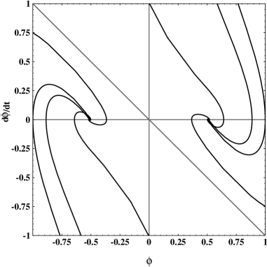
FIG. 6.: Phase space trajectories for $H_{0}=0.2$

In the first case the phase space trajectories converge to either of the two non-zero values of $\phi$ and is not an attractor like solution as the asymptotic nature of the solution depends on the initial conditions. But in the second case, however, the trajectories converge to $\phi=0$, ${\dot{\phi}}=0$ independent of the initial conditions and ,the de-Sitter solution is an attractor for this case.

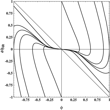
FIG. 7.: Phase space trajectories for $H_{0}=0.4$

IV Conclusion

The most important conclusion is that models with a self-interacting scalar field and a matter fluid having a negative pressure in addition to its positive equilibrium pressure can produce a scenario for the cosmological evolution in which one can have an inflationary phase to begin with, an accelerated phase at late times (like the present era) and a decelerating phase in-between. Recently Lopez and Matos [25] have shown that this kind of complete history for the scale factor can be described by a hyperbolic potential. But the physical origin of such potential is still not well known. But here we have shown that such kind of behaviour for the scale factor can be generated with a potential given in (22),which has been widely used by many authors for inflationary models.

The behaviour of $\rho$ and $\rho_{\phi}$ in our model shows that although in early universe, $\rho$ is greater than $\rho_{\phi}$ which is necessary for different physical phenomena like nucleosynthesis and structure formation etc, in the late times, $\rho_{\phi}$ starts dominating. This feature explains the missing energy density and also the ration of two energy densities becomes a constant in late time showing the “tracking nature”.

One should note that both the assumptions (8) and (16) play crucial role in our model. Given a barotropic equation of state between $\rho$ and $p$ one can not assume (8) and (16) at the same time if the dissipative pressure $\pi$ is zero in our model as t hat will lead to an over-determined problem ( the number of unknowns will be less than the number of independent equations). Even if one assumes these two condition one can check that will lead to an negative equilibrium pressure which is not desirable. H ence the existence of dissipative pressure also plays an important role in our model.

We have also studied the general equation of motion for the scalar field (equation (24)) for the potential (22) and have shown that for the choices of constant for which the potential is minimum at $\phi=0$, the phase space diagram exhibit a attractor behaviour towards the asymptotic de-sitter solution.

We want to mention that previously tracker and attractor solutions have been studied for scalar fields having inverse power law, exponential, cosine potential. But in all of these cases the equation of state $w$ is a constant in radiation era as well as in a matter dominated era. It was later shown by Pietro and Demaret  [18] that these kind of potential with a constant $w$ is not consistent with the field equations. In our case, the equation of state for the scalar field $w$ is not a constant but it varies with the cosmic evolution and approaches towards -1 asymptotically showing the existence of a cosmological constant in late times.

REFERENCES

- [1] Electronic address: anjan@mri.ernet.in
- [2] Electronic address: indrajit@mri.ernet.in
- [3] Electronic address: seshadri@mri.ernet.in
- [4] J. P. Ostriker and P. J. Steinhardt, Nature, 377, 600,(1995).
- [5] P. de Bernardis et al, Nature, 404, 955, (2000).
- [6] S. Perlmutter et.al., astro-ph/971221; A. G. Riess et.al, astro-ph/9805201.
- [7] N.A.Bahcall, J.P.Ostriker, S.Perlmutter and P.J.Steinhardt, Science, 284, 1481 (1988)
- [8] V.Sahni and A.Starobinsky, Int. J. Mod. Phys. D to appear (2000) astro-ph/9904398.
- [9] R.R.Caldwell, R.dave and P.J.Steinhardt, Phys. Rev. Lett, 80, 1582 (1998)
- [10] P.J.E.Peebles and B.Ratra, Astrophys.J.Lett., 325, L17, (1988); P.G.Ferreira and M.Joyce, Phys.Rev.Lett., 79, 4740 (1987); E.J.Copeland, A.R.Liddle and D.Wands, Phys.Rev.D, 57, 4686 (1988)
- [11] P.J. Steinhardt, L.Wang and I.Zlatev, Phys.Rev.Lett., 59, 123504 (1999)
- [12] I.Zlatev, L.Wang and P.J.Steinhardt, Phys.Rev.Lett., 82, 896 (1999).
- [13] V.Sahni and L.Wang, astro-ph/9910097
- [14] L.A.U.Lopez and T.Matos, astro-ph/0003364
- [15] J.P.Uzan, Phys.Rev.D, 59, 123510 (1999)
- [16] T.D. Saini, S. Raychauchaudhury, V. Sahni and A.A. Starobinsky, Phys.Rev.Lett, 85, 1162 (2000).
- [17] P.G.Ferreira and M.Joyce, Phys.Rev.D, 58, 023503 (1998); B. Ratra and P.J.E. Peebles, Phys. Rev. D, 37, 3406 (1988); T.Barreiro, E.J.Copeland and N.J.Nunes astro-ph/9910214.
- [18] Elisa De Pietro and Jacques Demaret gr-qc/9908071.
- [19] D.N.Spergel and P.J.Steinhardt Phys.Rev.Lett, 82, 896 (1999); J.P.Ostriker astro-ph/9912548; S.Hannestad astro-ph/9912558; B.Moore et.al Astrophys.J 535, L21 (2000).
- [20] L.P.Chimento, Alejandro S.Jakubi and Diego Pavon Phys.Rev.D 52, 063509 (2000).
- [21] W.Zimdahl, D.J.Schwarz, A.B.Balakin and D.Pavon Astro-Ph/0009353.
- [22] N.Banerjee and S.Sen Phys.Rev.D57, 4614 (1998); L.P.Chimento, V.Mendez and N.Zuccala, Int.J.Mod.Phys.D. 5, 313 (1996).
- [23] L. Chimento, V. Mendez and N. Zuccala, Class. Quantum Grav. 16 3749 (1999).
- [24] D.Lyth and A.Riotto Phys.Rep. 314 (1999).
- [25] L.Arturo Urena-Lopez and Tonatiuh Matos, astro-ph/0003364