Estimating Hawking radiation for exotic black holes

Abstract

We study about an approximation method of the Hawking radiation. We analyze an massless scalar field in exotic black hole backgrounds models which have peculiar properties in black hole thermodynamics (monopole black hole in SO(3) Einstein-Yang-Mills-Higgs system and dilatoic black hole in Einstein-Maxwell-dilaton system). A scalar field is assumed not to be couple to matter fields consisting of a black hole background. Except for extreme black holes, we can well approximate the Hawking radiaition by ‘black body’ one with Hawking temperature estimated at a radius of a critical impact parameter.

The Hawking radiaition[1] around black holes has been discussed for many years concerning various aspects, e.g., as $\gamma$-ray sources of the early universe[2] or vacuum polarization of charged black holes [3], etc. But as for black holes with non-Abelian hair [4, 5, 6, 7, 8, 9, 10], it has been less investigated because many of them are only obtained numerically that it takes much works compared with ones of analytically obtained. But we need to investigate for many reasons. Particularly, a monopole black hole which was found in SO(3) Einstein-Yang-Mill-Higgs (EYMH) system [11, 12, 13, 14] is important because it is one of the counterexample of the black hole no hair conjecture[15]. Moreover, if we consider the evaporation process of the Reissner-Nortström (RN) black hole, it may become a monopole black hole and the final product (a regular gravitating monopole) could be a good candidate for the remnant of the Hawking radiation in such a system.

From such view points, we study an approximation method of the Hawking radiation which may reduce our labor and discuss its validity in this paper. Throughout this paper we use units $c=\hbar=1$. Notations and definitions as such as Christoffel symbols and curvature follow Misner-Thorne-Wheeler[16].

We consider two models in which black hole solutions have peculiar properties in black hole thermodynamics.

(I) The SO(3) EYMH model as

$$S=\int d^{4}x\sqrt{-g}\left[\frac{R}{2\kappa^{2}}+L_{m}\right],$$ (1)

where $\kappa^{2}\equiv 8\pi G$ with $G$ being Newton’s gravitational constant. $L_{m}$ is the Lagrangian density of the matter fields which are written as

$$L_{m}=-\frac{1}{4}F^{a}_{\mu\nu}F^{a\mu\nu}-\frac{1}{2}(D_{\mu}\Phi^{a})(D^{\mu}\Phi^{a})-\frac{\lambda}{4}(\Phi^{a}\Phi^{a}-v^{2})^{2}\ .$$ (2)

$F^{a}_{\mu\nu}$ is the field strength of the SU(2) YM field and expressed by its potential $A^{a}_{\mu}$ as

$$F^{a}_{\mu\nu}=\partial_{\mu}A^{a}_{\mu}-\partial_{\nu}A^{a}_{\nu}+e\epsilon^{abc}A^{b}_{\mu}A^{c}_{\nu},$$ (3)

with a gauge coupling constant $e$. $\Phi^{a}$ is a real triplet Higgs field and $D_{\mu}$ is the covariant derivative:

$$D_{\mu}\Phi^{a}=\partial_{\mu}\Phi^{a}+e\epsilon^{abc}A^{b}_{\mu}\Phi^{c}.$$ (4)

The parameters $v$ and $\lambda$ are the vacuum expectation value and a self-coupling constant of the Higgs field, respectively.

(II) The Einstein-Maxwell-dilaton (EMD) model as

$$S=\frac{1}{2\kappa^{2}}\int d^{4}x\sqrt{-g}\left[R-2(\nabla\phi)^{2}-e^{-2\alpha\phi}F^{2}\right],$$ (5)

where $\phi$ and $F$ are a dilaton field and U(1) gauge field, respectively.

For black hole solutions, we assume that a space-time is static and spherically symmetric, in which case the metric is written as

$$ds^{2}=-f(r)e^{-2\delta(r)}dt^{2}+f(r)^{-1}dr^{2}+r^{2}d\Omega^{2},$$ (6)

where $f(r)=1-2Gm(r)/r$. We consider spacetime, which have a regular horizon and is asymptotically flat. In such a background spacetime, we consider a neutral and massless scalar field which does not couple to the matter fields such as the YM field or the Higgs field. The eq. of motion is described by the Klein-Gordon equation as

$$\Phi_{,\mu}^{\ ;\mu}=0.$$ (7)

This equation is separable, and we should only solve the radial equation

$$\frac{d^{2}\chi}{d{r}^{\ast 2}}+\chi\left[\omega^{2}-V^{2}\right]=0,$$ (8)

where

$$V^{2} \equiv \frac{f}{re^{2\delta}}\left\{\frac{l(l+1)}{r}-f\delta^{\prime}+\frac{2(m-m^{\prime}r)}{r^{2}}\right\},$$ (9)

$$\frac{dr}{dr^{\ast}} \equiv fe^{-\delta},$$ (10)

where ^′ denote $d/dr$ and $\chi$ is only the function of $r$.

The energy emission rate of Hawking radiation is given by

$$\Xi=\frac{1}{2\pi}\sum_{l=0}^{\infty}(2l+1)\int_{0}^{\infty}\frac{\Gamma(\omega)\omega}{e^{\omega/T_{H}}-1}d\omega,$$ (11)

where $l$ and $\Gamma(\omega)$ are the angular momentum and the transmission probability in a scattering problem for the scalar field $\Phi$. $\omega$ and $T_{H}$ are the energy of the particle and the Hawking temperature respectively. Note that $\Xi\equiv-dM/dt$.

The transmission probability $\Gamma$ can be calculated by solving radial equation (8) numerically under the boundary condition

$$\chi\rightarrow Ae^{-i\omega r^{\ast}}+Be^{i\omega r^{\ast}}\ \ (r^{\ast}\rightarrow\infty),$$ (12)

$$\chi\rightarrow e^{-i\omega r^{\ast}}\ \ (r^{\ast}\rightarrow-\infty),$$ (13)

where $\Gamma$ is given as $1/|A|^{2}$. As we see the dominant contribution for the Hawking radiation is $l=0$, because the contribution of the higher modes are suppressed by the centrifugal barrier. In what follows, we ignore the contributions from $l\geq 2$. Since the systematic error caused by it is below $1\%$, this does not affect the discussion below. The evaporation process of the monopole black hole and the dilatonic black holes were discussed numerically in [17] and in [18], respectively.

In this note, we study an approximation method of the Hawking radiation and check how accurate it is. Naively speaking, the Hawking radiation is a blackbody radiation with the temperature $T_{H}$. Then we may believe that $T_{H}$ mostly contributes to the Hawking radiation and determines the evaporation rate of a black hole. However we have another factor, i.e., transmission amplitude $\Gamma$. Since $\Gamma$ depends on the energy of the particle, we have to solve a radial equation and integrate (11). Moreover, we have to solve the background spacetime numerically for non-Abelian black holes. It would be rather a troublesome task.

But since the emission is of a blackbody nature, we may be able to estimate it by Stefan’s law[19] as $\Xi_{BB}\equiv\pi^{3}R_{eff}^{2}T_{H}^{4}/30$. The unknown is the effective radius $R_{eff}$. It has been suggested that for a Schwarzschild black hole, $R_{eff}$ is given by the photon orbit with some energy $E$ and angular momentum $L\equiv g_{ab}\Psi^{a}u^{b}$, where $\Psi^{a}$ and $u^{b}$ is the rotational Killing field and the 4-velocity, respectively. Although such a formula provides a good approximation in a Schwarzschild background, one may wonder whether it is still valid for exotic black holes, which have an envelope outside of the event horizon.

Starting with metric (6) and considering a massless particle in such a background, we find the maximum point of the effective potential $V_{eff}$ defined by

$$V_{eff}\equiv\frac{L^{2}}{2r^{2}}\left(1-\frac{2Gm(r)}{r}\right),$$ (14)

and then the effective radius as

$$R_{eff}\equiv\frac{L}{E}=\left(\frac{R^{3}}{R-2m(R)}\right)^{1/2}e^{\delta(R)},$$ (15)

where $R$ is the radial cordinate where $V_{eff}$ takes its maximum value. $R_{eff}$ is determined by the critical value of the “impact parameter” below which any “photon” sent toward the black hole can not escape. Using this effective radius, we define $\Xi_{BB}\equiv\pi^{3}R_{eff}^{2}T_{H}^{4}/30$ as a blackbody approximation.

First, we examine how well we can approximate by this method in monopole and RN black holes. We show a relation between the Hawking temperature $T_{H}$ and the ratio $\Xi/\Xi_{BB}$ in Fig. 1. We choose as $\lambda/e^{2}=0.1$, $v/M_{pl}=0.05$. The arrow in this diagram shows the direction of the smaller mass, which corresponds to that of the evaporating process. We find a quick turn below the point $A$ which corresponds to the sign change of the specific heat. Our calculation ends at $Q/Q_{max}=0.99$ where $Q_{max}$ is a maximum charge. As for other parameter choice of $\lambda$ and $v$, we obtain similar results. We summerize the results as follows.

(i) For more generic cases, the approximation is very good, but it becomes wrong near the extreme limit.

(ii) The temperature is not a good measure for the validity of this approximation. For example, if we have two solutions with the same temperature as in Fig. 1, a near-extreme solution gives worse result.

What condition should be imposed for good approximation? To clarify this, we consider the EMD model in which exact black hole solutions are obtained[20]. One of the reason to choose this model is the thermodynamical properties of the black hole depends on the coupling $\alpha$. Particularly, $\alpha$ changes the temperature and the shapes of the effective potential near the extreme solution. Roughly speaking, we may think its validity by two factors, steepness of the effective potential and the temperature which determines the frequency of particles which contribute to the emission rate.

We show shapes of the potentials for (a) $\alpha=0$ (b) $\alpha=1$ and (c) $\alpha=2$ in terms of $r^{\ast}$ in Fig. 2[21]. The parameters $Q/Q_{max}$ are chosen to be $0$, $0.84$, $0.89$, $0.94$, $0.99$ in (a) and (b) and to be $0$, $0.81$, $0.86$, $0.9$, $0.95$ in (c), respectively. As we increase $\alpha$, the difference from the Schwarzschild black hole increases near the extreme limit, i.e., the shapes of the potential becomes steep and the temperature becomes high. So its a competition between steepness of the potential which makes approximation wrong and the increasing temperature which improves the approximation.

We show the relation between $Q/Q_{max}$ and $\Xi/\Xi_{BB}$ for $\alpha=0$, $0.5$, $1.0$, $1.5$, $2.0$ in Fig. 3. For $Q/Q_{max}\mbox{\raisebox{-4.30554pt}{$\stackrel{{\scriptstyle\textstyle<}}{{\textstyle\sim}}$}}0.8$, $\Xi/\Xi_{BB}-1$ is about $0.06$, and it seems to be rather universal. But for $Q/Q_{max}\mbox{\raisebox{-4.30554pt}{$\stackrel{{\scriptstyle\textstyle>}}{{\textstyle\sim}}$}}0.8$, results depend on $\alpha$ remarkably. It may seem strange because the value $\Xi/\Xi_{BB}$ near the extreme solution does not monotonically increase by the increase of $\alpha$ (The order for ‘good’ approximation is $\alpha=2.0$, $1.5$, $0.0$, $1.0$, $0.5$.), but we can interpret it easily.

We show the relation between $T_{H}$ and $\Xi/\Xi_{BB}$ in Fig. 4 for the same parameters in Fig. 3. The arrows show the direction to the evaporation process. If we compare the $\Xi/\Xi_{BB}$ for fixed $T_{H}$, it monotonically depends on the ‘steepness’ of the potential which can be evaluated using $R_{eff}$ because it decreases when $V_{eff}$ becomes steep. Moreover, $R_{eff}$ can be the criterion for evaluating the curvature radius of the spacetime. Since $T_{H}$ is the good indicator of the mean frequency, to see $T_{H}R_{eff}$ would reveal the validity of the geometric optics approximation as was already pointed out in [19].

We show $T_{H}R_{eff}$ in terms of $Q/Q_{max}$ in Fig. 5. One can see that $T_{H}R_{eff}$ resembles to the $\Xi/\Xi_{BB}$. For the geometric optics approximation to be justified, it is usually demanded that $T_{H}R_{eff}$ should be far larger than $1$. But this figure shows that $\Xi_{BB}$ could work even in the case $T_{H}R_{eff}\sim 0.2$. It is surprising that this crude approximation provide such good results and it may provide the effective way to evaluate the Hawking radiation.

ACKOWLEDGEMENTS

Special Thanks to J. Koga, T. Torii and T. Tachizawa for useful discussions. T. T is thankful for financial support from the JSPS (No. 106613).

FIG. 1.: The ratio between the Hawking radiation and the black body approximation $\Xi/\Xi_{BB}$ in terms of the Hawking temperature $T_{H}/eM_{pl}^{2}$ for $\lambda/e^{2}=0.1$, $v/M_{pl}=0.05$. We show the RN black hole as dotted lines and the monopole black hole as solid lines. The point $A$ correspond to the change of the sign of the specific heat. We can find that though $\Xi_{BB}$ differs from $\Xi$ about $6\%$, its difference seems rather universal except below the point $A$.

FIG. 2.: Shapes of the potential $V_{eff}$ in terms of $r^{\ast}$ for (a) $\alpha=0$ (b) $\alpha=1$ (c) $\alpha=2$. For the parameter $Q/Q_{max}$, we choose to be $0$, $0.84$, $0.89$, $0.94$, $0.99$ in (a) and (b) and to be $0$, $0.81$, $0.86$, $0.9$, $0.95$ in (c). Note that for large $\alpha$, the shapes of the potential extremely change near the extreme limit.

FIG. 3.: The ratio between the Hawking radiation and the black body approximation $\Xi/\Xi_{BB}$ in terms of $Q/Q_{max}$ for dilatonic black holes for $\alpha=0$, $0.5$, $1$, $1.5$, $2$ which shows that near the extremal limit, $\Xi/\Xi_{BB}$ change rapidly.

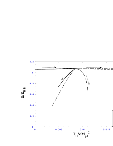
FIG. 4.: The ratio between the Hawking radiation and the black body approximation $\Xi/\Xi_{BB}$ in terms of Hawking temperature $T_{H}/eM_{pl}^{2}$ for the same solutions in Fig. 3. The arrows show the decrease of the gravitational mass if the electric charge is fixed. This may suggests that the approximation becomes invalid for the decrease of $T_{H}$ or approaching the extreme black hole.

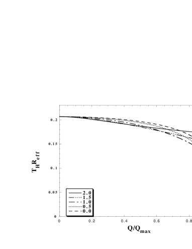
FIG. 5.: $T_{H}R_{eff}$ in terms of $Q/Q_{max}$ which shows that this can be the indicator to evaluate the validity of the approximation.

REFERENCES

- [1] S. W. Hawking, Nature 248, 30 (1974); Commun. Math. Phys. 43, 199 (1975).
- [2] D. N. Page and S. W. Hawking, Astrophys. J. 206, 1 (1976).
- [3] W. T. Zaumen, Nature 247, 530 (1974); G. W. Gibbons, Comm. Math. Phys. 44, 245 (1975).
- [4] As a review paper see K. Maeda, Journal of the Korean Phys. Soc. 28, S468, (1995), and M. S. Volkov and D. V. Gal’tsov, hep-th/9810070.
- [5] M. S. Volkov and D. V. Galt’sov, Pis’ma Zh. Eksp. Theor. Fiz. 50, 312 (1989); P. Bizon, Phys. Rev. Lett. 64, 2844 (1990); H. P. Künzle and A. K. Masoud-ul-Alam, J. Math. Phys. 31, 928 (1990).
- [6] K. Maeda, T. Tachizawa, T. Torii and T. Maki, Phys. Rev. Lett. 72, 450 (1994); T. Torii, K. Maeda and T. Tachizawa, Phys. Rev. D. 51, 1510 (1995).
- [7] S. Droz, M. Heusler and N. Straumann, Phys. Lett. B 268, 371 (1991).
- [8] B. R. Greene, S. D. Mathur and C. M. O’Neill, Phys. Rev. D 47, 2242 (1993).
- [9] H. Luckock and I. G. Moss, Phys. Lett. B 176, 341 (1986); H. Luckock, in String theory, quantum cosmology and quantum gravity, integrable and conformal invariant theories, eds. H. de Vega and N. Sanchez, (World Scientific, Singapore, 1986), p. 455.
- [10] T. Torii and K. Maeda, Phys. Rev. D 48, 1643 (1993).
- [11] P. Breitenlohner, P. Forgács and D. Maison, Nucl. Phys. B 383, 357 (1992); ibid. 442, 126 (1995).
- [12] K. -Y. Lee, V. P. Nair and E. Weinberg, Phys. Rev. Lett. 68, 1100 (1992); Phys. Rev. D 45, 2751 (1992); Gen. Relativ. Gravit. 24, 1203 (1992).
- [13] P. C. Aichelberg and P. Bizon, Phys. Rev. D. 48, 607 (1993).
- [14] T. Tachizawa, K. Maeda and T. Torii, Phys. Rev. D. 51, 4054 (1995).
- [15] P. Bizon, Acta. Phys. Pol. B 25, 877 (1994).
- [16] C. W. Misner, K. S. Thorne and J. A. Wheeler, Gravitation (Freeman, New York 1973).
- [17] T. Tamaki and K. Maeda, gr-qc/9910024.
- [18] J. Koga and K. Maeda, Phys. Rev. D. 52, 7066 (1995).
- [19] R. M. Wald, General Relativity (Chicago Press, Chicago and London 1984).
- [20] G.W. Gibbons and K. Maeda, Nucl. Phys. B 298, 741 (1988); D. Garfinkle, G. T. Horowitz and A. Strominger, Phys. Rev. D 43, 3140 (1991).
- [21] We use the same notation as in [18].