On the existence and convergence of polyhomogeneous expansions of zero-rest-mass fields.

Abstract

The convergence of polyhomogeneous expansions of zero-rest-mass fields in asymptotically flat spacetimes is discussed. An existence proof for the asymptotic characteristic initial value problem for a zero-rest-mass field with polyhomogeneous initial data is given. It is shown how this non-regular problem can be properly recast as a set of regular initial value problems for some auxiliary fields. The standard techniques of symmetric hyperbolic systems can be applied to these new auxiliary problems, thus yielding a positive answer to the question of existence in the original problem.

1 Introduction

The analysis of the asymptotic behaviour of asymptotically flat spacetimes and the diverse fields propagating on it has been carried out by assuming that both the gravitational field and the test fields (e.g. zero-rest-mass fields) are smooth at the boundary of the unphysical (i.e. conformally rescaled) spacetime manifold (null infinity, ${I}$) [7, 8, 10]. This smoothness at null infinity implies that the fields in the physical spacetime manifold have the peeling behaviour. However, this assumption may be too strong for a number of physical applications (see for example [2] and references within). In particular, the case for the so-called polyhomogeneous spacetimes and zero-rest-mass fields has been rised [1, 2, 14, 16, 15, 17]. A generic peeling (smooth) field possesses an analytic expansion around null infinity (given by $\Omega=0$). By contrast, the expansions of polyhomogeneous fields around ${I}$ are Laurent-like (so that the field in the physical spacetime is non-peeling), and also contain powers of $\ln$.

So far, the study of polyhomogeneous fields has been carried out assuming that the diverse fields admit expansions of the required form. However, the expansions are formal in the sense that the convergence (and hence the existence and uniqueness) of the series has not been discussed. This point, so many times overlooked, is of fundamental importance. It could be well the case that none of the formal expansions converge!

The objective of this article is to provide a first step towards the understanding of the convergence of polyhomogeneous fields. Here, I analyse the possible convergence of a polyhomogeneous spin-1 zero-rest-mass field (Maxwell field) propagating on an asymptotically simple spacetime. The spin-1 zero-rest-mass field has been chosen in order to ease the discussion and the calculations, but the treatment here discussed can be directly extended to the case of say, a spin-2 field. It is also expected that similar techniques can be used to analyse the analogous question for the gravitational field. However, in that case one should expect a number of complications. Furthermore, again for concreteness, only the simplest case of spin-1 zero-rest-mass fields will be discussed: the so-called minimally polyhomogeneous. This case contains all the difficulties one could expect from the generic polyhomogeneous situation, but the algebra is much simpler!

The question of the convergence of the polyhomogeneous expansions will be tackled by posing an asymptotic characteristic initial value problem for the minimally polyhomogeneous spin-1 zero-rest-mass field, and proving that such a problem has a (unique) solution in a given neighbourhood of the spacetime which is polyhomogeneous (i.e. the solution has convergent polyhomogeneous expansion in the given neighbourhood).

2 Preliminaries, notation, conventions

Let $(\widetilde{{M}},\widetilde{g}_{ab})$ be an asymptotically simple spacetime. It will be assumed that null infinity is smooth (non-polyhomogeneous). Let $({M},g_{ab})$ be the unphysical spacetime obtained by means of the conformal rescaling $g_{ab}=\Omega^{2}\widetilde{g}_{ab}$. The spacetime will be taken to be completely known. In particular this means that the asymptotic expansions of the spin coefficients, and the tetrad functions are known. Let $\mathcal{N}_{0}$ be the initial (future oriented) null hypersurface, and let $\mathcal{Z}_{0}$ be its intersection with future null infinity, $\mathcal{Z}_{0}=\mathcal{N}_{0}\cap{I}^{+}$. Following Penrose & Rindler’s notation, $\approx$ will denote equality at null infinity.

To describe the spacetime and the different fields involved, I will make use of the coordinates and null tetrad described by Friedrich & Stewart. In their original version, these coordinates and null tetrad were used to describe the spacetime between two intersecting null hypersurfaces [13, 12]. Here they are adapted to describe the region of spacetime in the causal past of the intersection of future null infinity (${I}^{+}$), and a future oriented null hypersurface. The construction is of interest in itself, and its highlights are given for the sake of reference.

The physical spacetime $(\widetilde{{M}},\widetilde{g}_{ab})$ is asymptotically flat, thus $\mathcal{Z}_{0}$ has the topology of the 2-sphere, $\mathcal{S}^{2}$. Let $p$ be an arbitrary point of $\mathcal{Z}_{0}$, and let $\gamma$ and $\gamma^{\prime}$ be the null generators of $\mathcal{N}_{0}$ and ${I}^{+}$ through $p$ respectively. A null tetrad $\{l^{a},n^{a},m^{a},\overline{m}^{a}\}$ at $p$ can be chosen such that $m^{a}$ and $\overline{m}^{a}$ span $\mbox{T}_{p}(\mathcal{Z}_{0})$, and $l^{a}$ and $n^{a}$ are tangent to $\gamma$ and $\gamma^{\prime}$ respectively. One can also choose an arbitrary coordinate system, $(x^{\alpha})$, at $\mathcal{Z}_{0}$. Let $u$ (retarded time) be a parameter along the null geodesic generators $\gamma^{\prime}$ of ${I}^{+}$, such that $u=0$ at $p$. Note that in principle $u$ is not an affine parameter. Repeating this construction for different points,$p$, one obtains a scalar field that vanishes precisely at $\mathcal{Z}_{0}$. The coordinates $(x^{\alpha})$ can now be extended to the remainder of ${I}^{+}$ by requiring the coordinates to be constant along the generators of ${I}^{+}$. In this way we have constructed a coordinate chart $(u,x^{\alpha})$ for ${I}^{+}$ valid at least around $\mathcal{Z}_{0}$. One can undertake an analogous construction for the generators $\gamma$ of $\mathcal{N}_{0}$, obtaining a parameter $v$ (advanced time) such that at $p\in\mathcal{Z}_{0}$, $v=0$. Again, the parameter $v$ is not affine in principle. Thus, one ends up with a coordinate chart $(v,x^{\alpha})$ for $\mathcal{N}_{0}$.

Now, on ${I}^{+}$ there is a 1-parameter family of spacelike hypersurfaces, $\mathcal{S}_{u}$ (cuts) on which $u$ is constant. For each $\mathcal{S}_{u}$ there is a unique null hypersurface $\mathcal{N}_{u}$ containing $\mathcal{S}_{0}$ ($\mathcal{S}_{u}\subset\mathcal{N}_{u}$) extending into the interior of the unphysical spacetime. This yields a foliation of the spacetime by null hypersurfaces at least close to ${I}^{+}$ —note that the foliation could give rise to caustics and cusps. Similarly, one can obtain another 1-parameter family of null hypersurfaces $\mathcal{N}^{\prime}_{v}$ for which $v$ is constant and that intersect $\mathcal{N}_{0}$. In particular one has that $\mathcal{N}_{0}^{\prime}={I}^{+}$. The coordinates $(x^{\alpha})$ can now also be extended to the interior of the spacetime by requiring them to be constant along the null generators of $\mathcal{N}_{u}$. Note that $(x^{\alpha})$ are not constant along the generators of the $\mathcal{N}_{v}^{\prime}$ foliation (except for ${I}^{+}$) for the null vectors $l^{a}$ and $n^{a}$ which will be taken as tangent to the null generators of $\mathcal{N}_{u}$ and $\mathcal{N}_{v}^{\prime}$ respectively do not in general commute.

To extend the null tetrad defined in $\mathcal{Z}_{0}$, one begins by defining $l_{a}$ on ${M}$ by $l_{a}=\nabla_{a}u$. Therefore $l^{a}$ is tangent to the null generators of $\mathcal{N}_{0}$, and is parallel to the $l^{a}$ already defined at $\mathcal{Z}_{0}$. A boost on the null tetrad defined at $\mathcal{Z}_{0}$ can be used to make the two vectors equal. Thus, there exists a scalar function $Q$ such that $l^{a}\partial_{a}=Q\partial_{v}$. It can be shown that $Q=\mathcal{O}(1)$. Next, the $n_{a}$ is defined on ${M}$ by $n_{a}=Q^{-1}\partial_{v}$, so that $n^{a}$ is tangent to the null generators of $N_{v}^{\prime}$ and the normalisation condition $l^{a}n_{a}=1$ is satisfied. Together with $n^{a}n_{a}=0$ this implies, $n^{a}\partial_{a}=\partial_{u}+c^{\alpha}\partial_{\alpha}$. Due to the constancy of the $(x^{\alpha})$ coordinates along the generators of ${I}^{+}$, one has that $C^{\alpha}\approx 0$.

Following the standard NP notation, let $D=l^{a}\nabla_{a}$ and $\Delta=n^{a}\nabla_{a}$. The vector $m^{a}$ defined so far only on $\mathcal{Z}_{0}$ is propagated onto the remaining of ${I}^{+}$ via the equation $\Delta m^{a}=-\tau n^{a}$. Finally $m^{a}$ is propagated from ${I}^{+}$ to the interior of ${M}$ via $Dm^{a}=-\overline{\pi}l^{a}$. This together with the nullity and orthogonality requirements imply that $m^{a}\partial_{a}=\xi^{\alpha}\partial_{\alpha}$.

Hence, the aforediscussed null tetrad has the form:

$$l^{a}=Q\delta^{a}_{v},$$ (1)

$$n^{a}=\delta^{a}_{u}+C^{\alpha}\delta_{\alpha}^{a},$$ (2)

$$m^{a}=\xi^{\alpha}\delta_{\alpha}^{a},$$ (3)

$$\overline{m}^{a}=\overline{\xi}^{\alpha}\delta_{\alpha}^{a},$$ (4)

where $C^{\alpha}\approx 0$, and $Q$, $\xi^{\alpha}$ are of order $\mathcal{O}(1)$. From this tetrad construction one also deduces that $\kappa=\nu=0$, $\rho=\overline{\rho}$, $\mu=\overline{\mu}$, $\epsilon=0$, $\tau=\overline{\alpha}+\beta$ in ${M}$. In particular one also has that all the spin coefficients with the exception of $\sigma$ vanish at ${I}^{+}$: that is, they are of order $\mathcal{O}(\Omega)$. On the other hand, $\sigma$ is $\mathcal{O}(1)$.

Finally, notice that the aforediscussed construction fixes also the associated spin basis $\{o^{A},\iota^{A}\}$.

2.1 Polyhomogeneous zero-rest-mass fields

A spin-s zero-rest-mass field is a totally symmetric spinor field ($\phi_{AB\cdots C}=\phi_{(AB\cdots C)}$), satisfying:

$$\nabla^{AA^{\prime}}\phi_{AB\cdots C}=0,$$ (5)

where the indices $AB\cdots C$ number $2s$. In order to ease the discussion, in this article we will restrict ourselves to spin 1 zero-rest-mass fields (Maxwell field). The extension of the results to spin 2 fields (linear gravity) is direct. The components of the spin 1 zero-rest-mass field in the aforementioned spin basis are: $\phi_{0}=\phi_{AB}o^{A}o^{B}$, $\phi_{1}=\phi_{AB}o^{A}\iota^{B}$, $\phi_{2}=\phi_{AB}\iota^{A}\iota^{B}$.

Let us consider zero-rest-mass fields belonging to $C^{\infty}_{loc}({M})$, i.e. fields that are infinite differentiable (smooth) in the interior of the unphysical spacetime ($\stackrel{{\scriptstyle\circ}}{{{M}}}=\widetilde{{M}}$) but need not to be so at the boundary (${I}$) of the spacetime; this is the meaning of the $loc$ label. In particular our attention will be centered on the so-called polyhomogeneous fields, which are $C^{\infty}_{loc}({M})$ zero-rest-mass fields with asymptotic expansions in terms of powers of a particular parameter (e.g. the conformal factor, and affine parameter of outgoing null geodesics, a luminosity parameter, an advanced time), and powers of the logarithm.

The most general polyhomogeneous spin-1 zero-rest-mass field is of the form,

$$\widetilde{\phi}_{0}=\phi_{0}^{2}\Omega^{2}+\phi_{0}^{3}\Omega^{3}+\cdots,$$ (6)

$$\widetilde{\phi}_{1}=\phi_{1}^{2}\Omega^{2}+\phi_{1}^{3}\Omega^{3}+\cdots,$$ (7)

$$\widetilde{\phi}_{2}=\phi_{2}^{1}\Omega+\phi_{2}^{2}\Omega^{2}+\cdots,$$ (8)

where the $\phi_{n}^{i}$’s are polynomials in $z=\ln\Omega$ with coefficients in $C^{\omega}(\mbox{{\SYM R}}\times\mathcal{S}^{2})$. It is customary to require absolute convergence of the polyhomogeneous series and its derivatives to all orders [2].

Note that the field defined by equations (6)-(8) is clearly non-peeling. A peeling field should behave like $\phi_{n}=\mathcal{O}(\Omega^{(3-n)})$. Furthermore, looking at the spin-1 zero-rest-mass field in the unphysical (conformally rescaled) spacetime one has,

$$\phi_{0}=\phi_{0}^{2}\Omega^{-1}+\phi_{0}^{3}+\cdots,$$ (9)

$$\phi_{1}=\phi_{1}^{2}+\phi_{1}^{3}\Omega+\cdots,$$ (10)

$$\phi_{2}=\phi_{2}^{1}+\phi_{2}^{2}\Omega+\cdots,$$ (11)

so that the field is not regular (diverges!) at ${I}^{+}$ (where $\Omega=0$), first because of the term $\phi_{0}^{2}\Omega^{-1}$, and also because of the presence of logarithmic terms in $\phi_{1}^{2}$.

In order to ease the discussion, the discussion in this article will be reduced to the case of the so-called minimally polyhomogeneous fields. An extension to more general polyhomogeneous fields can be easily done. A minimally polyhomogeneous spin-1 zero-rest-mass field is of the form (in the physical spacetime):

$$\widetilde{\phi}_{0}=\phi_{0}^{2,0}\Omega^{2}+\left(\phi_{0}^{3,1}\ln\Omega+\phi_{0}^{3,0}\right)\Omega^{3}+\cdots,$$ (12)

$$\widetilde{\phi}_{1}=\left(\phi_{1}^{2,1}\ln\Omega+\phi_{1}^{2,0}\right)\Omega^{2}+\cdots,$$ (13)

$$\widetilde{\phi}_{2}=\phi_{0}^{1,0}\Omega+\cdots,$$ (14)

which in the unphysical spacetime looks like,

$$\phi_{0}=\phi_{0}^{2,0}\Omega^{-1}+\left(\phi_{0}^{3,1}\ln\Omega+\phi_{0}^{3,0}\right)+\cdots,$$ (15)

$$\widetilde{\phi}_{1}=\left(\phi_{1}^{2,1}\ln\Omega+\phi_{1}^{2,0}\right)+\cdots,$$ (16)

$$\widetilde{\phi}_{2}=\phi_{0}^{1,0}+\left(\phi_{2}^{2,1}\ln\Omega+\phi_{2}^{2,0}\right)\Omega\cdots.$$ (17)

Using the “constraint equations”, i.e. the $D$-Maxwell equations one can deduce several relations connecting the diverse coefficients of the different components of the spin-1 zero-rest-mass field. In particular one has that

$$\phi_{1}^{2,1}=\overline{\eth}\phi_{0}^{2,0},$$ (18)

where $\overline{\eth}$ is the ethbar differential operator (see for example [9]). This relation will be used later.

So far, the asymptotic expansions have been in $\Omega$. However, it can be seen that,

$$\Omega=a(u,x^{\alpha})v+\cdots,$$ (19)

so that one could alternatively use the retarded time as the expansion parameter. This will be done in the remainder of the article. One can even redefine $a(u,x^{\alpha})$ so that $a(u,x^{\alpha})=1$.

A minimally polyhomogeneous field contains at the most first powers of $\ln$. If one provides $\widetilde{\phi}_{0}$ on an initial null hypersurface $\widetilde{\mathcal{N}}_{0}$, and the coefficients $\phi_{1}^{2,0}$ at $x^{0}=0$ and $\phi_{2}^{1,0}$ for all times, one can use the equations (22) and (23) on to obtain the components $\widetilde{\phi}_{1}$ and $\widetilde{\phi}_{2}$ on $\widetilde{\mathcal{N}}_{0}$, and then the evolution equations (20) and (21) to generate the field by “slices”. This procedure allows us to calculate formal polyhomogeneous expansions for the zero-rest-mass field. As mentioned previously in the introduction, the question to be investigated here regards the convergence of such formal polyhomogeneous expansions, i.e. we want to know if such fields exist, at least for a region of the spacetime very close to the initial null hypersurface $\mathcal{N}_{0}$.

3 Symmetric hyperbolicity and the asymptotic characteristic initial value problem

The question of the convergence of the polyhomogeneous expansions of the zero-rest-mass fields discussed in the previous section will be addressed by posing a so-called asymptotic characteristic initial value problem, i.e. an initial value problem with initial data given on a future oriented null hypersurface (a characteristic of the zero-rest-mass field equations), and on future null infinity (which, by the way is also a characteristic of the field equations). Once a suitable initial value problem has been posed, an existence result will be proven. This existence result will exhibit the convergence of the polyhomogeneous series. The aforesaid initial value problem is non-regular in a sense to be clarified later. Hence the standard techniques used to prove existence results for analytic fields cannot be directly used. Some manipulations will have to be carried. In order to understand the rationale behind the forthcoming discussion, the standard regular problem is briefly reviewed.

3.1 The initial value problem with regular initial data

Under the tetrad choice described in the previous sections, the spin-1 zero rest-mass field equations (aka source-free Maxwell equations) are given by:

$$\Delta\phi_{0}-\delta\phi_{1}=(2\gamma-\mu)\phi_{0}-2\tau\phi_{1}+\sigma\phi_{2},$$ (20)

$$\Delta\phi_{1}-\delta\phi_{2}=-2\mu\phi_{1}+(2\beta-\tau)\phi_{2},$$ (21)

$$D\phi_{2}-\overline{\delta}\phi_{1}=-\lambda\phi_{0}+2\pi\phi_{1}+\rho\phi_{2},$$ (22)

$$D\phi_{1}-\overline{\delta}\phi_{0}=(\pi-2\alpha)\phi_{0}+2\rho\phi_{1}.$$ (23)

Recall that the zero-rest-mass fields are totally symmetric, and thus in our case $\phi_{AB}o^{A}\iota^{B}=\phi_{AB}\iota^{A}o^{B}$. Therefore the system (20)-(23) is overdetermined: 4 equations for 3 complex components. This difficulty is overcome by discarding the last equation (23). Then, one has to verify that this equation is implied by the other ones if it held initially. This can be done by defining,

$$\Phi=D\phi_{1}-\overline{\delta}\phi_{0}-(\pi-2\alpha)\phi_{0}-2\rho\phi_{1}.$$ (24)

Using the field equations, the commutators and the Ricci identities (NP field equations), it is not difficult to show that,

$$\partial_{u}\Phi=0.$$ (25)

Thus, if equation (23) held initially, it will also held for later retarded times.

The principal part (symbol) of the reduced system (20)-(22) is contained in the terms

$$\Delta\phi_{0}-\delta_{1},$$ (26)

$$\Delta\phi_{1}-\delta_{2},$$ (27)

$$D\phi_{2}-\overline{\delta}\phi_{1},$$ (28)

and can be written concisely in a matricial way as $A^{a}\phi_{b,a}$ where $\phi=(\phi_{0},\phi_{1},\phi_{2})$, and

$$A^{u}=\left(\begin{array}[]{ccc}1&0&0\\ 0&1&0\\ 0&0&0\end{array}\right),$$ (29)

$$A^{v}=\left(\begin{array}[]{ccc}0&0&0\\ 0&0&0\\ 0&0&Q\end{array}\right),$$ (30)

and

$$A^{\alpha}=\left(\begin{array}[]{ccc}C^{\alpha}&0&0\\ 0&C^{\alpha}&-\xi^{\alpha}\\ 0&-\overline{\xi}^{\alpha}&0\end{array}\right).$$ (31)

Whence the reduced system (20)-(22) is clearly symmetric hyperbolic [12].

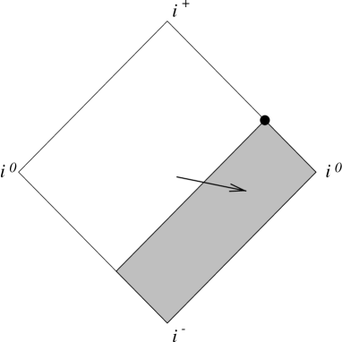
Figure 1: The asymptotic characteristic initial value problem for a zero rest-mass-field in an asymptotically simple spacetime.

Given suitable initial data on a future oriented null hypersurface $\mathcal{N}_{0}$ and on future null infinity ${I}^{+}$ one would like to obtain to obtain the spin-1 zero-rest-mass field to the past of the two initial hypersurfaces $J^{-}({I}^{+}\cup\mathcal{N}_{0})$. This is the asymptotic characteristic initial value problem. Alternatively one could give initial data on a past oriented null hypersurface $\mathcal{N}_{0}^{\prime}$ and on ${I}^{-}$ and reconstruct the field on $J^{+}({I}^{-}\cup\mathcal{N}_{0}^{\prime})$. For the sake of concreteness, here I will restrict to the first possibility.

From the structure of the principal part of the spin-1 zero-rest-mass field equations, one finds that the right way of setting such an asymptotic characteristic initial value problem for $\phi_{AB}$ is set by prescribing:

1. $\phi_{0}$ on $\mathcal{N}_{0}$,

2. $\phi_{1}$ on $\mathcal{Z}_{0}=\mathcal{N}_{0}\cap{I}^{+}$,

3. and $\phi_{2}$ on ${I}^{+}$.

If the initial data on $\mathcal{N}_{0}$ ($\phi_{0}$) peels, i.e. $\widetilde{\phi}_{0}=\mathcal{O}(\Omega^{3})$ or alternatively $\phi_{0}=\mathcal{O}(1)$), then $\phi_{0}$ is bounded at ${I}^{+}$, and one has a regular asymptotic characteristic initial value problem. Furthermore, if the data on $\mathcal{N}_{0}$ is analytic with respect to v, and the data on ${I}^{+}$ is analytic with respect to u, one can make use of Duff [4] and Friedrich’s techniques [5] theorem and prove that there is a unique analytic ($C^{\omega}$) solution to the posed initial value problem. The idea behind the proof is to construct another system of partial differential equations whose solutions can be shown to exist, be analytic and with an expansion that majorises the formal series solutions of the original system of equations. This implies the analyticity (and existence) of the solutions. In order to implement this construction the different terms in the equations are required to be analytic as well. The Duff-Friedrich’s construction works for quasilinear equations. Here, the situation is much simpler as the zero-rest-mass field equations are linear.

Further refinements can be implemented in order to show existence for the case when the initial data is $C^{\infty}$ rather than analytic [11, 6]. In such a case the field is found to be $C^{\infty}$. However, these further results may not concern us here.

3.2 The non-regular initial value problem

So much for the so-called regular initial value problem. What happens if the initial data over $\mathcal{N}_{0}$ is non-peeling, like for instance $\phi_{0}=\phi_{0}^{2,0}v^{-1}+\cdots$? As discussed elsewhere [17], such initial data gives rise to logarithms in the asymptotic expansions of the remaining components of the zero-rest-mass field spinor $\phi_{AB}$, and in $\phi_{0}$ itself for later times, even in the case where the logarithmic terms were not present in the initial data. An initial value problem with this kind of data that is not bounded at ${I}^{+}$, and henceforth it will be called non-regular.

In the case that concerns us here, that of a minimally polyhomogeneous spin-1 zero-rest-mass field, the non-regular nature of $\phi_{0}$ and $\phi_{1}$ at ${I}^{+}$ precludes us from setting an initial value problem as the one discussed above, and using directly Duff and Friedrich’s techniques.

Assume for a moment that we have a polyhomogeneous spin-1 zero-rest-mass field. Due to the absolute convergence of the formal series expansion, one can reshuffle the terms and write:

$$\phi_{0}=\stackrel{{\scriptstyle(1)}}{{\phi}}_{0}\ln v+\stackrel{{\scriptstyle(0)}}{{\phi}}_{0},$$ (32)

$$\phi_{1}=\stackrel{{\scriptstyle(1)}}{{\phi}}_{1}\ln v+\stackrel{{\scriptstyle(0)}}{{\phi}}_{1},$$ (33)

$$\phi_{2}=\stackrel{{\scriptstyle(1)}}{{\phi}}_{2}\ln v+\stackrel{{\scriptstyle(0)}}{{\phi}}_{2},$$ (34)

where the coefficients $\stackrel{{\scriptstyle(1)}}{{\phi}}_{n}$ and $\stackrel{{\scriptstyle(0)}}{{\phi}}_{n}$ are completely logarithm free! Asymptotically one has that

$$\begin{array}[]{ccc}\left\{\begin{array}[]{l}\widetilde{\stackrel{{\scriptstyle(1)}}{{\phi}}}_{0}=\mathcal{O}(\Omega^{3})\\ \widetilde{\stackrel{{\scriptstyle(1)}}{{\phi}}}_{1}=\mathcal{O}(\Omega^{2})\\ \widetilde{\stackrel{{\scriptstyle(1)}}{{\phi}}}_{2}=\mathcal{O}(\Omega^{2})\end{array}\right.&\mbox{ or }&\left\{\begin{array}[]{l}\stackrel{{\scriptstyle(0)}}{{\phi}}_{0}=\mathcal{O}(1)\\ \stackrel{{\scriptstyle(0)}}{{\phi}}_{1}=\mathcal{O}(1)\\ \stackrel{{\scriptstyle(0)}}{{\phi}}_{2}=\mathcal{O}(\Omega)\end{array}\right.\end{array}$$ (35)

and that

$$\begin{array}[]{ccc}\left\{\begin{array}[]{l}\widetilde{\stackrel{{\scriptstyle(0)}}{{\phi}}}_{0}=\mathcal{O}(\Omega^{2})\\ \widetilde{\stackrel{{\scriptstyle(0)}}{{\phi}}}_{1}=\mathcal{O}(\Omega^{2})\\ \widetilde{\stackrel{{\scriptstyle(0)}}{{\phi}}}_{2}=\mathcal{O}(\Omega^{1})\end{array}\right.&\mbox{ or }&\left\{\begin{array}[]{l}\stackrel{{\scriptstyle(0)}}{{\phi}}_{0}=\mathcal{O}(\Omega^{-1})\\ \stackrel{{\scriptstyle(0)}}{{\phi}}_{1}=\mathcal{O}(1)\\ \stackrel{{\scriptstyle(0)}}{{\phi}}_{2}=\mathcal{O}(1)\end{array}\right.\end{array}$$ (36)

for the other auxiliary field.

Thus, upon substitution on the field equations (20)-(22), one obtains the following equations for the auxiliary field,

$$\Delta\!\!\stackrel{{\scriptstyle(1)}}{{\phi}}_{0}-\delta\!\!\stackrel{{\scriptstyle(1)}}{{\phi}}_{1}=(2\gamma-\mu)\stackrel{{\scriptstyle(1)}}{{\phi}}_{0}-2\tau\stackrel{{\scriptstyle(1)}}{{\phi}}_{1}+\sigma\stackrel{{\scriptstyle(1)}}{{\phi}}_{2},$$ (37)

$$\Delta\!\!\stackrel{{\scriptstyle(1)}}{{\phi}}_{1}-\delta\!\!\stackrel{{\scriptstyle(1)}}{{\phi}}_{2}=-2\mu\stackrel{{\scriptstyle(1)}}{{\phi}}_{1}+(2\beta-\tau)\stackrel{{\scriptstyle(1)}}{{\phi}}_{2},$$ (38)

$$D\!\!\stackrel{{\scriptstyle(1)}}{{\phi}}_{2}-\overline{\delta}\!\!\stackrel{{\scriptstyle(1)}}{{\phi}}_{1}=-\lambda\stackrel{{\scriptstyle(1)}}{{\phi}}_{0}+2\pi\stackrel{{\scriptstyle(1)}}{{\phi}}_{1}+\rho\stackrel{{\scriptstyle(1)}}{{\phi}}_{2},$$ (39)

$$D\!\!\stackrel{{\scriptstyle(1)}}{{\phi}}_{1}-\overline{\delta}\!\!\stackrel{{\scriptstyle(1)}}{{\phi}}_{0}=(\pi-2\alpha)\stackrel{{\scriptstyle(1)}}{{\phi}}_{0}+2\rho\stackrel{{\scriptstyle(1)}}{{\phi}}_{1}.$$ (40)

which are in fact identical to the spin-1 zero-rest-mass field equations (20)-(23). Again, the system is overdetermined, and thus one discards the last equation.

In an ordinary asymptotic characteristic initial value problem, the initial data over $\mathcal{N}_{0}$ is prescribed, that is

$$\phi_{0}=\phi_{0}^{4,0}v^{-1}+\left(\phi_{0}^{5,1}\ln v+\phi_{0}^{5,0}\right)+\cdots,$$ (41)

is given. Thus, the value of

$$\stackrel{{\scriptstyle(1)}}{{\phi}}_{0}=\phi_{0}^{5,1}+\cdots,$$ (42)

at $\mathcal{N}_{0}$ is also known. Furthermore, as seen before $\phi_{1}^{2,1}=\overline{\eth}\phi_{0}^{2,0}$, and therefore we also know the value of $\stackrel{{\scriptstyle(1)}}{{\phi}}_{1}$ at $\mathcal{Z}_{0}$. Finally, as discussed previously,$\stackrel{{\scriptstyle(1)}}{{\phi}}_{2}=\mathcal{O}(v)$, and therefore $\stackrel{{\scriptstyle(1)}}{{\phi}}_{2}=0$ on ${I}^{+}$, i.e. the field is non-radiative . Consequently, we are are in the possession of all the ingredients needed to set an asymptotic characteristic value problem for the spin-1 zero-rest-mass field $\stackrel{{\scriptstyle(1)}}{{\phi}}_{AB}$. The initial data has been constructed out of the (non-regular) initial data for the original spin-1 zero-rest-mass field $\phi_{AB}$. Duff and Friedrich’s techniques allows us to state that there is an (unique) analytic solution for this initial value problem in a neighbourhood of $\mathcal{Z}_{0}$.

What happens with the other auxiliary field? In this case the equations are,

$$\Delta\!\!\stackrel{{\scriptstyle(0)}}{{\phi}}_{0}-\delta\!\!\stackrel{{\scriptstyle(0)}}{{\phi}}_{1}=(2\gamma-\mu)\stackrel{{\scriptstyle(0)}}{{\phi}}_{0}-2\tau\stackrel{{\scriptstyle(0)}}{{\phi}}_{1}+\sigma\stackrel{{\scriptstyle(0)}}{{\phi}}_{2},$$ (43)

$$\Delta\!\!\stackrel{{\scriptstyle(0)}}{{\phi}}_{1}-\delta\!\!\stackrel{{\scriptstyle(0)}}{{\phi}}_{2}=-2\mu\stackrel{{\scriptstyle(0)}}{{\phi}}_{1}+(2\beta-\tau)\stackrel{{\scriptstyle(0)}}{{\phi}}_{2},$$ (44)

$$D\!\!\stackrel{{\scriptstyle(0)}}{{\phi}}_{2}-\overline{\delta}\!\!\stackrel{{\scriptstyle(0)}}{{\phi}}_{1}+v^{-1}Q\stackrel{{\scriptstyle(1)}}{{\phi}}_{2}=-\lambda\stackrel{{\scriptstyle(0)}}{{\phi}}_{0}+2\pi\stackrel{{\scriptstyle(0)}}{{\phi}}_{1}+\rho\stackrel{{\scriptstyle(0)}}{{\phi}}_{2},$$ (45)

$$D\!\!\stackrel{{\scriptstyle(0)}}{{\phi}}_{1}-\overline{\delta}\!\!\stackrel{{\scriptstyle(0)}}{{\phi}}_{0}+v^{-1}Q\stackrel{{\scriptstyle(1)}}{{\phi}}_{1}=(\pi-2\alpha)\stackrel{{\scriptstyle(0)}}{{\phi}}_{0}+2\rho\stackrel{{\scriptstyle(0)}}{{\phi}}_{1}.$$ (46)

Note the presence of the extra terms $v^{-1}Q\!\!\stackrel{{\scriptstyle(1)}}{{\phi}}_{2}$ and $v^{-1}Q\!\!\stackrel{{\scriptstyle(1)}}{{\phi}}_{1}$. Thus the auxiliary field $\stackrel{{\scriptstyle(0)}}{{\phi}}_{AB}$ satisfies a kind of sourced Maxwell equations. The source happens to be precisely the vacuum field $\stackrel{{\scriptstyle(1)}}{{\phi}}_{AB}$. As it has been done before, one discards the last equation (46).

From a previous analysis, one knows that $\stackrel{{\scriptstyle(1)}}{{\phi}}_{2}=\mathcal{O}(v)$, and thus the whole new term in equation (45) is such that $v^{-1}Q\stackrel{{\scriptstyle(1)}}{{\phi}}_{2}=\mathcal{O}(1)$. Hence, it is regular at ${I}^{+}$. However, Duff and Friedrich’s techniques cannot be applied to the reduced system (43)-(45), as it is, for the initial data over the initial hypersurface $\mathcal{N}_{0}$ is not regular.

As discussed, $\stackrel{{\scriptstyle(0)}}{{\phi}}_{0}=\phi_{0}^{2,0}v^{-1}+\mathcal{O}(1)$. Substitution of this into equation (43) yields,

$$\partial_{u}\phi_{0}^{2,0}=0.$$ (47)

Therefore, the non-regular term is a constant of motion [17]. Let $\stackrel{{\scriptstyle(0)}}{{\phi}}_{0}=\phi_{0}^{2,0}v^{-1}+\stackrel{{\scriptstyle(0)}}{{\phi}}_{0*}$, with $\stackrel{{\scriptstyle(0)}}{{\phi}}_{0*}=\mathcal{O}(1)$, i.e. from a physical spacetime point of view the component $\stackrel{{\scriptstyle(0)}}{{\phi}}_{0*}=\mathcal{O}(1)$ satisfies the peeling behaviour. Substitution into equations (20)-(22) yields,

$$\Delta\!\!\stackrel{{\scriptstyle(0)}}{{\phi}}_{0*}-\delta\!\!\stackrel{{\scriptstyle(0)}}{{\phi}}_{1}=(2\gamma-\mu)\phi^{2,0}_{0}v^{-1}+(2\gamma-\mu)\stackrel{{\scriptstyle(0)}}{{\phi}}_{0*}-2\tau\stackrel{{\scriptstyle(0)}}{{\phi}}_{1}+\sigma\stackrel{{\scriptstyle(0)}}{{\phi}}_{2},$$ (48)

$$\Delta\!\!\stackrel{{\scriptstyle(0)}}{{\phi}}_{1}-\delta\!\!\stackrel{{\scriptstyle(0)}}{{\phi}}_{2}=-2\mu\stackrel{{\scriptstyle(0)}}{{\phi}}_{1}+(2\beta-\tau)\stackrel{{\scriptstyle(0)}}{{\phi}}_{2},$$ (49)

$$D\!\!\stackrel{{\scriptstyle(0)}}{{\phi}}_{2}-\overline{\delta}\!\!\stackrel{{\scriptstyle(0)}}{{\phi}}_{1}+v^{-1}Q\stackrel{{\scriptstyle(1)}}{{\phi}}_{2}=-\lambda\phi^{2,0}_{0}v^{-1}-\lambda\stackrel{{\scriptstyle(0)}}{{\phi}}_{0*}+2\pi\stackrel{{\scriptstyle(0)}}{{\phi}}_{1}+\rho\stackrel{{\scriptstyle(0)}}{{\phi}}_{2}.$$ (50)

Now, $\gamma=\mathcal{O}(v)$, $\mu=\mathcal{O}(v)$, and $\lambda=\mathcal{O}(v)$. Therefore, the new extra terms $(2\gamma-\mu)\phi^{2,0}_{0}v^{-1}$ and $-\lambda\phi^{2,0}_{0}v^{-1}$ are regular at ${I}^{+}$ and known. Moreover, they are also analytic at $v=0$. Therefore we have obtained a perfectly regular symmetric hyperbolic system for $\stackrel{{\scriptstyle(0)}}{{\phi}}_{0*}$, $\stackrel{{\scriptstyle(0)}}{{\phi}}_{1}$, and $\stackrel{{\scriptstyle(0)}}{{\phi}}_{2}$.

Furthermore, we also know the value of $\stackrel{{\scriptstyle(0)}}{{\phi}}_{0*}$ at the initial hypersurface $\mathcal{N}_{0}$ (obtainable from the non-regular initial value problem for $\phi_{AB}$). The value of $\stackrel{{\scriptstyle(0)}}{{\phi}}_{1}$ at $\mathcal{Z}_{0}$ is also known. Finally $\stackrel{{\scriptstyle(0)}}{{\phi}}_{2}\approx\phi_{2}$, and thus we also know the data on ${I}^{+}$. Consequently we have obtained a regular system of symmetric hyperbolic equations for the scalars $\stackrel{{\scriptstyle(0)}}{{\phi}}_{0*}$, $\stackrel{{\scriptstyle(0)}}{{\phi}}_{1}$, $\stackrel{{\scriptstyle(0)}}{{\phi}}_{2}$ with suitable initial data on which Duff and Friedrich’s ideas can be used. The conclusion is that there exists a neighbourhood of $\mathcal{Z}_{0}$ on which there exists an (unique) analytic solution ($C^{\omega}$) to the posed initial value problem. If $\stackrel{{\scriptstyle(0)}}{{\phi}}_{0*}$ is analytic in a neighbourhood of ${I}^{+}$ then clearly $\phi_{0}=\phi_{0}^{2,0}v^{-1}$ has a convergent Laurent expansion on the same neighbourhood.

So, we have seen that there exists a neighbourhood ${U}_{1}$ of $\mathcal{Z}_{0}$ for which the field $\stackrel{{\scriptstyle(1)}}{{\phi}}_{AB}$ is analytic (in $v$), and another neighbourhood ${U}_{0}$ for which the field $\stackrel{{\scriptstyle(0)}}{{\phi}}_{AB}$ has a Laurent expansion (again in $v$). Let ${U}={U}_{0}\cap{U}_{1}$. Thus, one can say that the non-regular asymptotic characteristic initial value problem for the zero-rest-mass field $\phi_{AB}=\stackrel{{\scriptstyle(0)}}{{\phi}}_{AB}+\stackrel{{\scriptstyle(1)}}{{\phi}}_{AB}\ln v$ has a (unique) solution in ${U}\!\!-\!\!{I}^{+}$ which is in fact polyhomogeneous. Note that althought the field is not well defined at ${I}^{+}$, the radiation field is well defined ($\phi_{2}$) as it is part of the regular initial data. Furthermore, it can be shown that the net electromagnetic charge of the field (as measured from null infinity) is also well defined.

These results can be sumarised in the form of the following

Theorem 1

Let $(\widetilde{{M}},\widetilde{g}_{ab})$ be a Ricci flat ($R_{ab}=0$) asymptotically simple spacetime, and let $({M},g_{ab})$ be the corresponding unphysical spacetime obtained by the conformal rescaling. Furthermore, let $\mathcal{N}_{0}$ be a future oriented null hypersurface in ${M}$ that intersects ${I}^{+}$ at $\mathcal{Z}_{0}$. Then there exist a neighbourhood ${U}$ of $\mathcal{Z}_{0}$ such that the non-regular asymptotic characteristic initial value problem for a spin-1 zero-rest-mass field with minimally polyhomogeneous data on $\mathcal{N}_{0}$ has a unique (polyhomogeneous) solution in ${U}\!\!-\!\!{I}^{+}$.

4 Conclusions

An existence result for the asymptotic characteristic initial value problem for a spin-1 zero-rest-mass field with polyhomogeneous initial data has been proved. The polyhomogeneous initial data is not bounded at ${I}^{+}$, and thus, the initial value problem is non-regular. This means essentially that standard existence theorems for symmetric hyperbolic equations cannot be directly used. However, as seen it possible to reformulate this non-regular initial value problem as two coupled initial value problems for some auxiliary fields. These auxiliary fields satisfy partial differential equations with regular initial data. Moreover, these auxiliary systems have the same principal part (symbol) as the spin-1 zero-rest-mass field.

The existence result shows that the polyhomogeneous structure of the initial data is preserved at least in a neighbourhood of $\mathcal{Z}_{0}$. And for the same price, one also settles the matter of the convergence of polyhomogeneous expansions for zero-rest-mass fields.

4.1 Further extensions

The proof given here is limited to minimally polyhomogeneous spin-1 zero-rest-mass field equations. A proof for an arbitrary polyhomogeneous spin-2 zero-rest-mass field (higher spins are not so interesting as the Buchdahl constraint has to be satisfied) follows using the same techniques. Arbitrary polyhomogeneity in the initial data means that further auxiliary fields and their respective systems should be included in the discussion. As it has been pointed out elsewhere, these auxiliary fields form a hierarchy. This hierarchy is such that the field equations for a given auxiliary field has the auxiliary field just above in the hierarchy as source term (cfr. with the equations for $\stackrel{{\scriptstyle(1)}}{{\phi}}_{AB}$ and $\stackrel{{\scriptstyle(0)}}{{\phi}}_{AB}$). The consideration of a spin-2 field rather than a spin-1 one would only increase the amount of algebra involved.

A much more interesting and natural extension of this work is to trying to apply similar techniques to polyhomogeneous gravitational fields. This would require the use of Friedrich’s regular conformal field equations, and a good understanding of the formal polyhomogeneous solutions to the aforementioned equations. These concerns will be and are the concern of future work.

References

- [1] L. Andersson & P. T. Chruściel, On “hyperboloidal” Cauchy data for vacuum Einstein equations and obstructions to smoothness of scri, Comm. Math. Phys. 161, 533 (1994).
- [2] P. T. Chruściel, M. A. H. MacCallum, & D. B. Singleton, Gravitational waves in general relativity XIV. Bondi expansions and the “polyhomogeneity” of , Phil. Trans. Roy. Soc. Lond. A 350, 113 (1995).
- [3] R. Courant & D. Hilbert, Methods of Mathematical Physics, volume II, John Wiley & Sons, 1962.
- [4] G. F. D. Duff, Mixed problems for linear systems of first order equations, Can. J. Math. 10, 127 (1958).
- [5] H. Friedrich, On the existence of analytic null asymptotically flat solutions of Einstein’s vacuum field equations, Proc. Roy. Soc. Lond. A 381, 361 (1982).
- [6] J. Kánnár, On the existence of solutions to the asymptotic characteristic initial value problem in general relativity, Proc. Roy. Soc. Lond. A 452, 945 (1996).
- [7] R. Penrose, Asymptotic properties of fields and space-times, Phys. Rev. Lett. 10, 66 (1963).
- [8] R. Penrose, Zero rest-mass fields including gravitation: asymptotic behaviour, Proc. Roy. Soc. Lond. A 284, 159 (1965).
- [9] R. Penrose & W. Rindler, Spinors and space-time. Volume 1. Two-spinor calculus and relativistic fields, Cambridge University Press, 1984.
- [10] R. Penrose & W. Rindler, Spinors and space-time. Volume 2. Spinor and twistor methods in space-time geometry, Cambridge University Press, 1986.
- [11] A. D. Rendall, Reduction of the characteristic initial value problem to the Cauchy problem and its application to the Einstein equations, Proc. Roy. Soc. Lond. A 427, 221 (1990).
- [12] J. Stewart, Advanced general relativity, Cambridge University Press, 1991.
- [13] J. M. Stewart & H. Friedrich, Numerical relativity. The characteristic initial value problem, Proc. Roy. Soc. Lond. A 384, 427 (1982).
- [14] J. A. Valiente Kroon, Conserved Quantities for polyhomogeneous spacetimes, Class. Quantum Grav. 15, 2479 (1998).
- [15] J. A. Valiente Kroon, A Comment on the Outgoing Radiation Condition and the Peeling Theorem, Gen. Rel. Grav. 31, 1219 (1999).
- [16] J. A. Valiente Kroon, Logarithmic Newman-Penrose Constants for polyhomogeneous spacetimes, Class. Quantum Grav. 16, 1653 (1999).
- [17] J. A. Valiente Kroon, Polyhomogeneity and zero-rest-mass fields with applications to Newman-Penrose constants, Class. Quantum Grav. 17, 605 (2000).