Exact Solutions to the Motion of Two Charged Particles in Lineal Gravity

R.B. Mann, D. Robbins

Dept. of Physics, University of Waterloo Waterloo, ONT N2L 3G1, Canada

T. Ohta

Department of Physics, Miyagi University of Education, Aoba-Aramaki, Sendai 980, Japan

and

M. Trott

Dept. of Physics, University of Toronto Toronto, ONT, Canada

PACS numbers: 13.15.-f, 14.60.Gh, 04.80.+z

We extend the canonical formalism for the motion of $N$-particles in lineal gravity to include charges. Under suitable coordinate conditions and boundary conditions the Hamiltonian is defined as the spatial integral of the second derivative of the dilaton field which is given as a solution to the constraint equations. For a system of two particles the determining equation of the Hamiltonian (a kind of transcendental equation) is derived from the matching conditions for the dilaton field at the particles’ position. The canonical equations of motion are derived from this determining equation.

For the equal mass case the canonical equations in terms of the proper time can be exactly solved in terms of hyperbolic and/or trigonometric functions. In electrodynamics with zero cosmological constant the trajectories for repulsive charges exhibit not only bounded motion but also a countably infinite series of unbounded motions for a fixed value of the total energy $H_{0}$, while for attractive charges the trajectories are simply periodic. When the cosmological constant $\Lambda$ is introduced, the motion for a given $\Lambda$ and $H_{0}$ is classified in terms of the charge-momentum diagram from which we can predict what type of the motion is realized for a given charge. In general the cosmological constant acts on the particles as a repulsive ($\Lambda>0$) or an attractive ($\Lambda<0$) potential. But for a certain range of $\Lambda<0$, small $q$ and small mass the trajectory shows a double peak structure due to an interplay among the induced momentum dependent $\Lambda$ potential, the gravitational attraction and the relativistic effect. For $\Lambda>0$, depending on the value of charge, only bounded motion or the infinite series of unbounded motion or both are realized.

Since in this theory the charge of each particle appears in the form $e_{1}e_{2}$ in the determining equation, the static balance condition in 1+1 dimensions turns out to be identical with the condition in Newtonian theory. We generalize this condition to non-zero momenta, obtaining the first exact solution to the static balance problem that does not obey the Majumdar-Papapetrou condition.

1 INTRODUCTION

The problem of determining the motion of a system of $N$ particles mutually interacting through specified forces is one that has attracted attention since the dawn of physics. We continue in this paper our previous explorations of this problem in two spacetime dimensions when the specified interactions are both gravitational and electromagnetic.

Our work here represents the first exact solution to include both interactions in a relativistic framework. Although an exact solution is known in three spatial dimensions for pure Newtonian gravity in the $N=2$ case, dissipation of energy in the form of gravitational radiation has obstructed progress toward obtaining exact solutions for the motion of $N$ bodies in the general theory of relativity, even when $N=2$.  However by reducing the number of spatial dimensions this obstruction disappears, at least in the vacuum. Apart from the absence of gravitational radiation, most (if not all) of the remaining conceptual features of relativistic gravity are retained, and so lower dimensional theories of gravity offer the hope of garnering insight into the nature of classical and quantum gravitation in a wide variety of physical situations.

For these reasons we have been investigating the $N$-body problem in two dimensional gravity for the past 3 years. We have chosen to work with a 2D theory that models 4D general relativity in that it sets the Ricci scalar equal to the trace of the stress-energy of prescribed matter fields and sources. Hence matter governs the evolution of spacetime curvature which reciprocally governs the evolution of matter [1]. This theory (sometimes referred to as $R=T$ theory) has a consistent Newtonian limit [1], a problematic limit in a generic $(1+1)$-dimensional theory of gravity theory [2]. When the stress-energy is that of a cosmological constant, the theory reduces to Jackiw-Teitelboim (JT) theory [3].

Working in the canonical formalism [4], we have so far been able to obtain exact solutions to the two body problem in the absence [5] and presence [6] of a cosmological constant. In this paper we extend these considerations to include charged bodies.  Specifically, we formulate the charged $N$-body problem in relativistic gravity by taking the matter action to be that of $N$ charged point-particles minimally coupled to gravity and electromagnetism. We extend the previous canonical formalism we developed for this action in $R=T$ lineal gravity [4] to include this case. When $N=2$ we obtain exact solutions for the motion of two bodies of unequal (and equal) charge and mass. In the slow motion, weak field limit the Hamiltonian we obtain coincides with that of Newtonian gravity with electromagnetism in $(1+1)$ dimensions.  We are also able to extend our solutions to include a cosmological constant $\Lambda$, so that in the limit where all bodies are massless and neutral, spacetime has constant curvature (ie the JT theory is obtained). Our solution is the first non-static exact solution to the charged 2-body problem in any relativistic theory of gravity.

Our exact solution to the $N=2$ case can be formulated in several ways. We derive an exact solution for the Hamiltonian as a function of the proper separation and the centre-of-inertia momentum of the charged bodies. We are also able to construct a solution in which the proper separation of the two charged point masses is given as a function of their mutual proper time in the equal mass case. If the masses are not equal our exact solution is given in terms of a time-coordinate that is not the proper time.

A scalar (dilaton) field must be included in the action [7] since the Einstein action is a topological invariant in (1+1) dimensions. Canonically reducing the action, we find that the Hamiltonian is given in terms of a spatial integral of the second derivative of the dilaton field, which is a function of the canonical variables of the particles (coordinates and momenta) and is determined from the constraint equations. The matching conditions of the solution to the constraint equations yield an equation which determines the Hamiltonian in terms of the remaining degrees of freedom of the system when $N=2$ . We refer to this transcendental equation as the determining equation, since it allows one to determine the Hamiltonian in terms of the centre of inertia momentum and proper separation of the bodies. From this Hamiltonian we can derive the canonical equations of motion. In the equal mass case we find that the separation and momentum are given by differential equations in terms of the proper time, and can be exactly solved in terms of hyperbolic and/or trigonometric functions.

Several different types of motion are expected in the 2 body case, depending upon the signs and magnitudes of the masses, charges, energy and other parameters (e.g. gravitational coupling constant, cosmological constant). If the charges are of opposite sign the particles will remain bounded, whereas if they are of the same sign either bounded or unbounded motion can occur for the same value of the total energy. For a given set of parameters there is in this case a countably infinite series of unbounded motions labelled by an integer $n$. A balance condition exists between the bounded and the unbounded cases, and reduces to the expected (Newtonian-like) static balance condition in the absence of particle momenta. We shall analyze these various states of motion, and discuss the transitions which occur between them. A cosmological constant can qualitatively change the motion, rendering bound states unbound and vice-versa. We find several surprising situations, including the diverging separation of the two bodies at finite proper time in the repulsive case, even for $\Lambda=0$. In the $\Lambda<0$ case the motion shows a double maximum behavior for a certain range of the parameters, which is a characteristic effect of the induced momentum dependent $\Lambda$ potential. For classification of the motion we utilize a charge-momentum diagram from which we can easily predict what type of the motion is realized for a given charge.

In the unequal mass case the proper time is no longer the same for the two particles, and a more careful analysis is necessary in order to describe the motion. We obtain phase space trajectories from the determining equation and explicit solutions for the proper separation in terms of a transformed time coordinate which reduces to the mutual proper time in the case of equal mass.

In Sec.II we describe the outline of the canonical reduction of the theory when the charges are included and define the Hamiltonian for the $N$- body system. In Sec.III we solve the constraint equations for the two-body case and get the determining equation of the Hamiltonian, from which the canonical equations of motion are explicitly derived. For the case of equal masses and arbitrary charges the explicit exact solutions to the canonical equations are given in Sec.IV. By using these exact solutions we analyze in Sec.V the motion for $\Lambda=0$ separately for four cases: attractive charges, small repulsive charges, large repulsive charges and $H<2m$. We analyze the motion of equal masses for $\Lambda\neq 0$ in Sec.VI for four possible combinations of the signs of $\Lambda$ and the charges, where we also develop the plots of phase space trajectories and the analysis of the explicit solutions in terms of the proper time, based on a classification given by a charge-momentum diagram. We treat the unequal mass case in Sec.VII. In Sec.VIII we investigate the static balance problem by using both the canonical equation and the determining equation. Sec.IX contains concluding remarks and directions for further work. The solution of the metric tensor, a linear approximation of the exact solutions and the causal relationships between particles in unbounded motion are given in Appendices.

2 CANONICALLY REDUCED HAMILTONIAN OF $N$-CHARGED PARTICLES

Our derviation of the canonically reduced Hamiltonian for charged particles is parallel to that given in the uncharged case [5, 8]. Here we briefly review this work, highlighting those aspects that are peculiar to the charged case.

The action integral for gravitational and electromagnetic fields coupled with $N$ charged point masses is

$$I = \int d^{2}x\left[\frac{1}{2\kappa}\sqrt{-g}g^{\mu\nu}\left\{\Psi R_{\mu\nu}+\frac{1}{2}\nabla_{\mu}\Psi\nabla_{\nu}\Psi+\frac{1}{2}g_{\mu\nu}\Lambda\right\}\right.$$ (1)

$$\makebox[20.00003pt]{}\left.-A_{\mu}{\cal F}_{\;\;,\nu}^{\mu\nu}+\frac{1}{4\sqrt{-g}}{\cal F}^{\mu\nu}{\cal F}^{\alpha\beta}g_{\mu\alpha}g_{\nu\beta}\right.$$

$$\makebox[20.00003pt]{}\left.+\sum_{a}\int d\tau_{a}\left\{-m_{a}\left(-g_{\mu\nu}(x)\frac{dz_{a}^{\mu}}{d\tau_{a}}\frac{dz_{a}^{\nu}}{d\tau_{a}}\right)^{1/2}+e_{a}\frac{dz_{a}^{\mu}}{d\tau_{a}}A_{\mu}(x)\right\}\delta^{2}(x-z_{a}(\tau_{a}))\right]\;,$$

where $\Psi$ is the dilaton field, $A_{\mu}$ and ${\cal F}^{\mu\nu}$ are the vector potential and the field strength, $g_{\mu\nu}$ and $g$ are the metric and its determinant, $R$ is the Ricci scalar, and $e_{a}$ and $\tau_{a}$ are the charge and the proper time of $a$-th particle, respectively, with $\kappa=8\pi G/c^{4}$. The symbol $\nabla_{\mu}$ denotes the covariant derivative associated with $g_{\mu\nu}$.

The field equations derived from the action (1) are

$$R-g^{\mu\nu}\nabla_{\mu}\nabla_{\nu}\Psi=0\;,$$ (2)

$$\frac{1}{2}\nabla_{\mu}\Psi\nabla_{\nu}\Psi-\frac{1}{4}g_{\mu\nu}\nabla^{\lambda}\Psi\nabla_{\lambda}\Psi+g_{\mu\nu}\nabla^{\lambda}\nabla_{\lambda}\Psi-\nabla_{\mu}\nabla_{\nu}\Psi=\kappa T_{\mu\nu}+\frac{1}{2}g_{\mu\nu}\Lambda\;,$$ (3)

$${\cal F}_{\;\;,\nu}^{\mu\nu}=\sum_{a}e_{a}\int d\tau_{a}\frac{dz_{a}^{\mu}}{d\tau_{a}}\delta^{2}(x-z_{a}(\tau_{a}))\;,$$ (4)

$$\frac{1}{\sqrt{-g}}{\cal F}_{\mu\nu}=\partial_{\mu}A_{\nu}-\partial_{\nu}A_{\mu}\;,$$ (5)

$$m_{a}\left[\frac{d}{d\tau_{a}}\left\{g_{\mu\nu}(z_{a})\frac{dz_{a}^{\nu}}{d\tau_{a}}\right\}-\frac{1}{2}g_{\nu\lambda,\mu}(z_{a})\frac{dz_{a}^{\nu}}{d\tau_{a}}\frac{dz_{a}^{\lambda}}{d\tau_{a}}\right]=e_{a}\frac{dz_{a}^{\nu}}{d\tau_{a}}\left\{A_{\nu,\mu}(z_{a})-A_{\mu,\nu}(z_{a})\right\}\;,$$ (6)

where the stress-energy due to the point masses and the electric field is

$$T_{\mu\nu}=\sum_{a}m_{a}\int d\tau_{a}\frac{1}{\sqrt{-g}}g_{\mu\sigma}g_{\nu\rho}\frac{dz_{a}^{\sigma}}{d\tau_{a}}\frac{dz_{a}^{\rho}}{d\tau_{a}}\delta^{2}(x-z_{a}(\tau_{a}))+\frac{1}{(-g)}\left\{{\cal F}_{\mu\alpha}{\cal F}_{\nu\beta}g^{\alpha\beta}-\frac{1}{4}g_{\mu\nu}{\cal F}_{\alpha\beta}{\cal F}^{\alpha\beta}\right\}\;,$$ (7)

recalling that in (1+1) dimensions no magnetic component of the field exists. Eq.(3) guarantees the conservation of $T_{\mu\nu}$. Inserting the trace of Eq.(3) into Eq.(2) yields

$$R-\Lambda=\kappa T_{\;\;\mu}^{\mu}\;.$$ (8)

Eqs.(4), (5), (6) and (8) form a closed sytem of equations for gravity, electromagnetism, and matter.

On transforming the action (1) to the canonical form we first rewrite the electromagnetic and the particle sectors in a form appropriate to the first-order formalism [9].

$$I_{E+P} = \int dx^{2}\left[-A_{\mu}{\cal F}_{\;\;,\nu}^{\mu\nu}+\frac{1}{4\sqrt{-g}}{\cal F}^{\mu\nu}{\cal F}^{\alpha\beta}g_{\mu\alpha}g_{\nu\beta}\right.$$ (9)

$$\left.+\sum_{a}\int d\tau_{a}\left\{\pi_{a\mu}\frac{dz_{a}^{\mu}}{d\tau_{a}}-\frac{1}{2}\lambda_{a}^{\prime}(\tau_{a})(\pi_{a\mu}\pi_{a\nu}g^{\mu\nu}+m_{a}^{2})+e_{a}\frac{dz_{a}^{\mu}}{d\tau_{a}}A_{\mu}(x)\right\}\delta^{2}(x-z_{a}(\tau_{a}))\right]\;,$$

where $\pi_{a}^{\mu}$ is essentially the four velocity of the particle and $\lambda_{a}^{\prime}$ is a Lagrange multiplier. The variations with respect to $A_{\mu}$ and ${\cal F}^{\mu\nu}$ lead to Eqs.(4) and (5), respectively, and those with respect to $\pi_{a\mu},z_{a}^{\mu}$ and $\lambda_{a}^{\prime}$ lead to

$$\frac{dz_{a}^{\mu}}{d\tau_{a}}-\lambda_{a}^{\prime}\pi_{a}^{\mu}=0\;,$$ (10)

$$\frac{d\pi_{a\mu}}{d\tau_{a}}+\frac{1}{2}\lambda_{a}^{\prime}\pi_{a\lambda}\pi_{a\nu}g_{\;\;,\mu}^{\lambda\nu}(z_{a})=e_{a}\frac{dz_{a}^{\nu}}{d\tau_{a}}\left\{A_{\nu,\mu}(z_{a})-A_{\mu,\nu}(z_{a})\right\}\;,$$ (11)

$$\pi_{a\mu}\pi_{a\nu}g^{\mu\nu}+m_{a}^{2}=0\;.$$ (12)

This set of three equations is equivalent to Eq.(6) when $\lambda_{a}^{\prime}=1/m_{a}$ is chosen.
By performing the integration over the parameter $\tau_{a}$ and setting

$$z_{a}^{\mu} = (t,z_{a})\;,\qquad\pi_{a\mu}=(\pi_{a0},\pi_{a})\;,$$

$$A_{\mu} = (-\varphi,A)\;,\qquad E={\cal F}^{01}\;,$$ (13)

$$\lambda_{a} = \lambda_{a}^{\prime}\frac{d\tau_{a}}{dz_{a}^{0}}|_{z_{a}^{0}(\tau_{a})=t}\;.$$ (14)

the action (9) becomes

$$I_{E+P} = \int d^{2}x\left[A\frac{\partial E}{\partial t}-\frac{1}{2}\sqrt{-g}E^{2}+\varphi\left\{\frac{\partial E}{\partial x}-\sum_{a}e_{a}\delta(x-z_{a}(t))\right\}\right.$$

$$\left.+\sum_{a}\frac{dz_{a}}{dt}(\pi_{a}+e_{a}A)\delta(x-z_{a}(t))+\sum_{a}\left\{\pi_{a0}-\frac{1}{2}\lambda(\pi_{a\mu}\pi_{a\nu}g^{\mu\nu}+m_{a}^{2})\right\}\delta(x-z_{a}(t))\right]\;.$$

Varying the Lagrange multipliers $\varphi$ and $\lambda_{a}$ yields the constraints

$$\frac{\partial E}{\partial x}=\sum_{a}e_{a}\delta(x-z_{a}(t))\;,$$ (16)

$$\pi_{a\mu}\pi_{a\nu}g^{\mu\nu}+m_{a}^{2}=0\;.$$ (17)

The solution to (16) is

$$E=\frac{1}{2}\partial_{x}\sum_{a}e_{a}|x-z_{a}(t)|\;.$$ (18)

In (1+1) dimensions the electric field has no independent degrees of freedom. When the charged particles move within a finite region $(|x|<L)$, the electric field in an outer region $(|x|>L)$ is $E=\pm\frac{1}{2}\sum_{a}e_{a}$. For a system of zero total charge the electric field vanishes in the outer region. As the solution to (17) we choose

$$\pi_{a0}=\frac{1}{g^{00}}\left\{-g^{01}\pi_{a}+\sqrt{(g^{01}\pi_{a})^{2}-g^{00}(g^{11}\pi_{a}^{2}+m_{a}^{2})}\right\}\;.$$ (19)

After the constraints are eliminated, the action (2) is

$$I_{E+P} = \int d^{2}x\left[\sum_{a}\pi_{a}\frac{dz_{a}}{dt}\delta(x-z_{a}(t))\right.$$

$$\left.+\sum_{a}\frac{1}{g^{00}}\left\{-g^{01}\pi_{a}+\sqrt{(g^{01}\pi_{a})^{2}-g^{00}(g^{11}\pi_{a}^{2}+m_{a}^{2})}\right\}\delta(x-z_{a}(t))-\frac{1}{2}\sqrt{-g}E^{2}(t,x)\right]\;.$$

From this expression we know that $\pi_{a}$ is the conjugate momentum to $z_{a}$ and hereafter we use the notation

$$p_{a}\equiv\pi_{a}\;.$$

Note that the variations of the action (2) with respect to $A$ and $E$ lead to

$$\makebox[30.00005pt]{}\frac{\partial E}{\partial t}+\sum_{a}e_{a}\frac{dz_{a}}{dt}\delta(x-z_{a}(t))=0\;,$$ (21)

$$\makebox[30.00005pt]{}\sqrt{-g}E=-\frac{\partial\varphi}{\partial x}-\frac{\partial A}{\partial t}\;.$$ (22)

Eq.(21) is automatically satisfied for the solution (18) to the constraint equation, in contrast to the (3+1) dimensional case where the corresponding equation is a true dynamical equation. Upon inserting the solution (18) into the action (2) all terms related to the components of $A_{\mu}$ cancel. Hence we need no longer consider $A_{\mu}$. Its solution, if desired, is straightforwardly obtained by solving (16) after fixing the gauge and obtaining the full solution of the metric.

Consider next the transformation of the gravity sector to canonical form. We decompose the scalar curvature in terms of the extrinsic curvature $K$ via

$$\sqrt{-g}R=-2\partial_{0}(\sqrt{\gamma}K)+2\partial_{1}[(N_{1}K-\partial_{1}N_{0})/\sqrt{\gamma}]\;,$$ (23)

where the metric is

$$ds^{2}=-N_{0}^{2}dt^{2}+\gamma\left(dx+\frac{N_{1}}{\gamma}dt\right)^{2}\;,$$ (24)

with $K=(2N_{0}\gamma)^{-1}(2\partial_{1}N_{1}-\gamma^{-1}N_{1}\partial_{1}\gamma-\partial_{0}\gamma)$, so that $\gamma=g_{11},N_{0}=(-g^{00})^{-1/2}$ and $N_{1}=g_{10}$. We then rewrite the gravity sector in first-order form . We find that the action (1) becomes

$$I=\int d^{2}x\left\{\sum_{a}p_{a}\dot{z}_{a}\delta(x-z_{a}(t))+\pi\dot{\gamma}+\Pi\dot{\Psi}+N_{0}R^{0}+N_{1}R^{1}\right\}\;,$$ (25)

where $\pi$ and $\Pi$ are conjugate momenta to $\gamma$ and $\Psi$, respectively, and

$$R^{0} = -\kappa\sqrt{\gamma}\gamma\pi^{2}+2\kappa\sqrt{\gamma}\pi\Pi+\frac{1}{4\kappa\sqrt{\gamma}}(\Psi^{\prime})^{2}-\frac{1}{\kappa}\left(\frac{\Psi^{\prime}}{\sqrt{\gamma}}\right)^{\prime}-\frac{1}{2}\sqrt{\gamma}(E^{2}-\frac{\Lambda}{\kappa})$$

$$-\sum_{a}\sqrt{\frac{p_{a}^{2}}{\gamma}+m_{a}^{2}}\;\delta(x-z_{a}(t))\;,$$

$$R^{1} = \frac{\gamma^{\prime}}{\gamma}\pi-\frac{1}{\gamma}\Pi\Psi^{\prime}+2\pi^{\prime}+\sum_{a}\frac{p_{a}}{\gamma}\delta(x-z_{a}(t))\;,$$ (26)

with the symbols $(\;\dot{}\;)$ and $(\;^{\prime}\;)$ denoting $\partial_{0}$ and $\partial_{1}$, respectively.

From the action (25) we obtain the set of equations

$$\dot{\pi} + N_{0}\left\{\frac{3\kappa}{2}\sqrt{\gamma}\pi^{2}-\frac{\kappa}{\sqrt{\gamma}}\pi\Pi+\frac{1}{8\kappa\sqrt{\gamma}\gamma}(\Psi^{\prime})^{2}+\frac{1}{4\sqrt{\gamma}}(E^{2}-\frac{\Lambda}{\kappa})\right.$$ (27)

$$\makebox[100.00015pt]{}\left.-\sum_{a}\frac{p_{a}^{2}}{2\gamma^{2}\sqrt{\frac{p_{a}^{2}}{\gamma}+m_{a}^{2}}}\;\delta(x-z_{a}(t))\right\}$$

$$+ N_{1}\left\{-\frac{1}{\gamma^{2}}\Pi\Psi^{\prime}+\frac{\pi^{\prime}}{\gamma}+\sum_{a}\frac{p_{a}}{\gamma^{2}}\;\delta(x-z_{a}(t))\right\}+N_{0}^{\prime}\frac{1}{2\kappa\sqrt{\gamma}\gamma}\Psi^{\prime}+N_{1}^{\prime}\frac{\pi}{\gamma}=0\;,$$

$$\dot{\gamma}-N_{0}(2\kappa\sqrt{\gamma}\gamma\pi-2\kappa\sqrt{\gamma}\Pi)+N_{1}\frac{\gamma^{\prime}}{\gamma}-2N_{1}^{\prime}=0\;,$$ (28)

$$R^{0}=0\;,$$ (29)

$$R^{1}=0\;,$$ (30)

$$\dot{\Pi}+\partial_{1}(-\frac{1}{\gamma}N_{1}\Pi+\frac{1}{2\kappa\sqrt{\gamma}}N_{0}\Psi^{\prime}+\frac{1}{\kappa\sqrt{\gamma}}N_{0}^{\prime})=0\;,$$ (31)

$$\dot{\Psi}+N_{0}(2\kappa\sqrt{\gamma}\pi)-N_{1}(\frac{1}{\gamma}\Psi^{\prime})=0\;,$$ (32)

$$\dot{p}_{a}+\frac{\partial N_{0}}{\partial z_{a}}\sqrt{\frac{p_{a}^{2}}{\gamma}+m_{a}^{2}}-\frac{N_{0}}{2\sqrt{\frac{p_{a}^{2}}{\gamma}+m_{a}^{2}}}\frac{p_{a}^{2}}{\gamma^{2}}\frac{\partial\gamma}{\partial z_{a}}-\frac{\partial N_{1}}{\partial z_{a}}\frac{p_{a}}{\gamma}$$

$$\makebox[20.00003pt]{}+N_{1}\frac{p_{a}}{\gamma^{2}}\frac{\partial\gamma}{\partial z_{a}}+\int dxN_{0}\sqrt{\gamma}E\frac{\partial E}{\partial z_{a}}=0\;,$$ (33)

$$\dot{z_{a}}-N_{0}\frac{\frac{p_{a}}{\gamma}}{\sqrt{\frac{p_{a}^{2}}{\gamma}+m_{a}^{2}}}+\frac{N_{1}}{\gamma}=0\;.$$ (34)

In the equations (33) and (34), all metric components ($N_{0}$, $N_{1}$, $\gamma$) are evaluated at the point $x=z_{a}$ and

$$\frac{\partial f}{\partial z_{a}}\equiv\left.\frac{\partial f(x)}{\partial x}\right|_{x=z_{a}}\;.$$

The quantities $N_{0}$ and $N_{1}$ are Lagrange multipliers which yield the constraint equations (29) and (30). The above set of equations can be proved to be equivalent to the set of equations (2), (3) and (6).

To proceed to the canonical reduction of the action (25) we have to eliminate the redundant variables by utilizing the constrant equations to fix the coordinate conditions. Noticing that the only linear terms in the constraint equations (29) and (30) are $\left(\Psi^{\prime}/\sqrt{\gamma}\right)^{\prime}$ and $\pi^{\prime}$, respectively, and the equations may be solved for these quantities, we can transform the total generator obtained from the end point variation into an approriate form to fix the coordinate conditions. Generalizing the procedure described in our previous papers [4, 5] for the case of $\Lambda=e_{a}=0$, we find that we can consistently choose the coordinate conditions 

$$\gamma=1\makebox[20.00003pt]{}\mbox{and}\makebox[20.00003pt]{}\Pi=0\;.$$ (35)

Eliminating the constraints, the action (25) reduces to

$$I=\int dx^{2}\left\{\sum_{a}p_{a}\dot{z}_{a}\delta(x-z_{a})-{\cal H}\right\}\;,$$ (36)

where the reduced Hamiltonian for the system of particles is defined by

$$H=\int dx{\cal H=-}\frac{1}{\kappa}\int{\cal\triangle}\Psi\;.$$ (37)

Here $\Psi$ is a function of $z_{a}$ and $p_{a}$ and is determined by solving the constraints which under the coordinate conditions (35) become

$$\triangle\Psi-\frac{1}{4}(\Psi^{\prime})^{2}+\kappa^{2}\pi^{2}+\frac{1}{2}(\kappa E^{2}-\Lambda)+\kappa\sum_{a}\sqrt{p_{a}^{2}+m_{a}^{2}}\delta(x-z_{a})=0\;,$$ (38)

$$2\pi^{\prime}+\sum_{a}p_{a}\delta(x-z_{a})=0\;.$$ (39)

The consistency of this canonical reduction is proved in an analogous way to the case of $\Lambda=e_{a}=0$ : namely the canonical equations of motion derived from the reduced Hamiltonian (37) are identical with the equations (33) and (34) [5, 8].

3 SOLUTION TO THE CONSTRAINT EQUATIONS AND THE HAMILTONIAN FOR A SYSTEM OF TWO PARTICLES

The standard approach for investigating the dynamics of particles is to get first an explicit expression of the Hamiltonian and to derive the equations of motion, from which the solution of trajectories are obtained. In this section we show how to derive the Hamiltonian from the solution to the constraint equations (38) and (39) and get the explicit Hamiltonian for a system of two charged particles. Since the electric field appears in the combination $(E^{2}-\Lambda/\kappa)$ in all equations we set

$$V(x)\equiv E^{2}-C\quad\mbox{and}\quad\Lambda_{e}\equiv\Lambda-\kappa C$$ (40)

with $C\equiv\frac{1}{4}(\sum_{a}e_{a})^{2}$. Thus $V(x)$ vanishes in the outer region and $\Lambda_{e}$ is an effective cosmological constant, which includes the contribution from the electric field. This latter situation arises from the well-known fact that in (1+1) dimensions the electromagnetic field strength is a 2-form, and so in compact spatial regions it contributes to the stress-energy tensor in the same manner as a cosmological constant, analogous to the way in which a 4-form behaves in 3+1 dimensions [10]. We shall later see that when $\Lambda_{e}$ vanishes we get the Hamiltonian which leads, in the limit $\kappa\rightarrow 0$, to the correct special-relativistic electrodynamics in (1+1) flat space-time.

We express equations (38) and (39) as

$$\triangle\Psi=\frac{1}{4}\left(\Psi^{\prime}\right)^{2}-\kappa^{2}\left(\chi^{\prime}\right)^{2}-\frac{1}{2}(\kappa V-\Lambda_{e})-\kappa\sum_{a}\sqrt{p_{a}^{2}+m_{a}^{2}}\delta(x-z_{a})\;,$$ (41)

$$\triangle\chi=-\frac{1}{2}\sum_{a}p_{a}\delta(x-z_{a})\;,$$ (42)

where we set $\chi^{\prime}=\pi$. Rewriting (41) as

$$(1+\frac{\Psi}{4})\triangle\Psi=\frac{1}{8}\triangle(\Psi^{2}-4\kappa^{2}\chi^{2})-\frac{1}{2}(\kappa V-\Lambda_{e})+\kappa^{2}\chi\triangle\chi-\kappa\sum_{a}\sqrt{p_{a}^{2}+m_{a}^{2}}\delta(x-z_{a})\;,$$ (43)

yields, upon insertion into the Right-hand side (RHS) of (37)

$$H = \sum_{a}\frac{\sqrt{p_{a}^{2}+m_{a}^{2}}}{1+\frac{1}{4}\Psi(z_{a})}+\frac{\kappa}{2}\sum_{a}\frac{p_{a}\chi(z_{a})}{1+\frac{1}{4}\Psi(z_{a})}+\frac{1}{2}\int dx\frac{V(x)}{1+\frac{1}{4}\Psi(x)}$$ (44)

$$-\frac{1}{8\kappa}\int dx\frac{1}{1+\frac{1}{4}\Psi(x)}\triangle\left(\Psi^{2}-4\kappa^{2}\chi^{2}+2\Lambda_{e}x^{2}\right)\;.$$

an expression which can also be obtained repeated iteration of the insertion of the RHS of (41) into the RHS of (37).

Defining $\phi$ by

$$\Psi=-4\ln|\phi|\;,$$ (45)

the constraints (41) and (42) for a two-particle system become

$$\triangle\phi-\frac{1}{4}\left\{\kappa^{2}\left(\chi^{\prime}\right)^{2}+\frac{\kappa}{2}V-\frac{1}{2}\Lambda_{e}\right\}\phi = \frac{\kappa}{4}\left\{\sqrt{p_{1}^{2}+m_{1}^{2}}\;\phi(z_{1})\delta(x-z_{1})\right.$$ (46)

$$\left.\quad+\sqrt{p_{2}^{2}+m_{2}^{2}}\;\phi(z_{2})\delta(x-z_{2})\right\}\;,$$

$$\triangle\chi=-\frac{1}{2}\left\{p_{1}\delta(x-z_{1})+p_{2}\delta(x-z_{2})\right\}\;.$$ (47)

The general solution to (47) is

$$\chi=-\frac{1}{4}\left\{p_{1}\mid x-z_{1}\mid+p_{2}\mid x-z_{2}\mid\right\}-\epsilon Xx+\epsilon C_{\chi}\;\;.$$ (48)

The factor $\epsilon$ ($\epsilon^{2}=1$) has been introduced in the constants $X$ and $C_{\chi}$ so that the T-inversion (time reversal) properties of $\chi$ are explicitly manifest. By definition, $\epsilon$ changes sign under time reversal and so, therefore, does $\chi$.

Consider first the case $z_{2}<z_{1}$, for which we may divide space into three regions: $z_{1}<x$ ((+) region), $z_{2}<x<z_{1}$ ((0) region) and $x<z_{2}$ ((-) region). In each region, $V$ and $\chi^{\prime}$ are constant:

$$V=\left\{\begin{array}[]{ll}0&\qquad\mbox{(+) region},\\ -\frac{1}{2}e_{1}e_{2}&\qquad\mbox{(0) region},\\ 0&\qquad\mbox{(-) region},\end{array}\right.$$ (49)

$$\chi^{\prime}=\left\{\begin{array}[]{ll}-\epsilon X-\frac{1}{4}(p_{1}+p_{2})&\makebox[30.00005pt]{}\mbox{(+) region},\\ -\epsilon X+\frac{1}{4}(p_{1}-p_{2})&\makebox[30.00005pt]{}\mbox{(0) region},\\ -\epsilon X+\frac{1}{4}(p_{1}+p_{2})&\makebox[30.00005pt]{}\mbox{(-) region}\;.\end{array}\right.$$ (50)

General solutions to the homogeneous equation $\triangle\phi-\frac{1}{4}\left\{\kappa^{2}\left(\chi^{\prime}\right)^{2}+\frac{\kappa}{2}V-\frac{1}{2}\Lambda_{e}\right\}\phi=0$ in each region are

$$\left\{\begin{array}[]{l}\phi_{+}(x)=A_{+}e^{\frac{1}{2}K_{+}x}+B_{+}e^{-\frac{1}{2}K_{+}x}\;,\\ \phi_{0}(x)=A_{0}e^{\frac{1}{2}K_{0}x}+B_{0}e^{-\frac{1}{2}K_{0}x}\;,\\ \phi_{-}(x)=A_{-}e^{\frac{1}{2}K_{-}x}+B_{-}e^{-\frac{1}{2}K_{-}x}\;,\end{array}\right.$$ (51)

where

$$\left\{\begin{array}[]{lll}K_{+}&=\sqrt{\kappa^{2}\left(X+\frac{\epsilon}{4}(p_{1}+p_{2})\right)^{2}-\frac{1}{2}\Lambda_{e}}&\qquad\mbox{(+) region}\;,\\ K_{0}&=\sqrt{\kappa^{2}\left(X-\frac{\epsilon}{4}(p_{1}-p_{2})\right)^{2}-\frac{\kappa}{2}e_{1}e_{2}-\frac{1}{2}\Lambda_{e}}&\qquad\mbox{(0) region}\;,\\ K_{-}&=\sqrt{\kappa^{2}\left(X-\frac{\epsilon}{4}(p_{1}+p_{2})\right)^{2}-\frac{1}{2}\Lambda_{e}}&\qquad\mbox{(-) region}\;.\end{array}\right.$$ (52)

For these solutions to be the actual solutions to Eq.(46) with delta function source terms, they must satisfy the following matching conditions at $x=z_{1},z_{2}$:

$$\phi_{+}(z_{1})=\phi_{0}(z_{1})=\phi(z_{1})\;,$$ (53a)

$$\phi_{-}(z_{2})=\phi_{0}(z_{2})=\phi(z_{2})\;,$$ (53b)

$$\phi^{\prime}_{+}(z_{1})-\phi^{\prime}_{0}(z_{1})=\frac{\kappa}{4}\sqrt{p^{2}_{1}+m^{2}_{1}}\phi(z_{1})\;,$$ (53c)

$$\phi^{\prime}_{0}(z_{2})-\phi^{\prime}_{-}(z_{2})=\frac{\kappa}{4}\sqrt{p^{2}_{2}+m^{2}_{2}}\phi(z_{2})\;.$$ (53d)

Since the magnitudes of both $\Psi$ and $\chi$ increase with increasing $|x|$, it is necessary to impose a boundary condition which guarantees that the surface terms which arise in transforming the action vanish and simultaneously preserves the finiteness of the Hamiltonian. From the iterative expression (44) we know that we may choose the boundary condition

$$\Psi^{2}-4\kappa^{2}\chi^{2}+2\Lambda_{e}x^{2}=C_{\pm}x\qquad\mbox{for (+) and (-) regions}$$ (54)

with $C_{\pm}$ being constants to be determined.

The above matching conditions accompanied by the boundary condition (54) determine the solution $\phi$ ( and also all coefficients) completely. The process of the calculation is quite analogous to the procedure in the previous paper [8], and we shall omit the details here. The compact expression of the $\phi$ solution is

$$\phi_{+} = \left(\frac{K_{1}}{{\cal M}_{1}}\right)^{\frac{1}{2}}\;e^{-\frac{1}{4}(K_{01}z_{1}-K_{02}z_{2})+\frac{1}{2}K_{+}(x-z_{1})}\;,$$

$$\phi_{0} = \frac{1}{4K_{0}}\;e^{-\frac{1}{4}(K_{01}z_{1}-K_{02}z_{2})}\left\{(K_{1}{\cal M}_{1})^{1/2}e^{-\frac{1}{2}K_{0}(x-z_{1})}+(K_{2}{\cal M}_{2})^{1/2}e^{\frac{1}{2}K_{0}(x-z_{2})}\right\}\;,$$ (55)

$$\phi_{-} = \left(\frac{K_{2}}{{\cal M}_{2}}\right)^{\frac{1}{2}}\;e^{-\frac{1}{4}(K_{01}z_{1}-K_{02}z_{2})-\frac{1}{2}K_{-}(x-z_{2})}\;,$$

where

$$K_{1} \equiv 2K_{0}+2K_{-}-\kappa\sqrt{p_{2}^{2}+m_{2}^{2}}\;,$$

$$K_{2} \equiv 2K_{0}+2K_{+}-\kappa\sqrt{p_{1}^{2}+m_{1}^{2}}\;,$$

$$K_{01} \equiv K_{0}-K_{+}+\frac{\kappa\epsilon}{2}p_{1}\;,$$ (56)

$$K_{02} \equiv K_{0}-K_{-}-\frac{\kappa\epsilon}{2}p_{2}\;,$$

$${\cal M}_{1} \equiv \kappa\sqrt{p_{1}^{2}+m_{1}^{2}}+2K_{0}-2K_{+}\;,$$

$${\cal M}_{2} \equiv \kappa\sqrt{p_{2}^{2}+m_{2}^{2}}+2K_{0}-2K_{-}\;,$$

and among these quantites there exists one relation

$$K_{1}K_{2}={\cal M}_{1}{\cal M}_{2}\;e^{K_{0}(z_{1}-z_{2})}\;,$$ (57)

which we refer to as the determining equation of $X$.

The Hamiltonian (37) becomes

$$H = -\frac{1}{\kappa}\int dx\triangle\Psi=\frac{4}{\kappa}\left[\frac{\phi^{\prime}}{\phi}\right]_{-\infty}^{\infty}$$ (58)

$$= \frac{2(K_{+}+K_{-})}{\kappa}\;\;.$$

Once the solution $X$ to (57) is obtained, the Hamiltonian is explicitly determined. Consequently (57) is the determining equation of the Hamiltonian.

Repeating the analysis for $z_{1}<z_{2}$ yields a similar solution with $p_{i}\rightarrow-p_{i}$ and so the full solution is obtained by replacing $p_{i}$ and $z_{1}-z_{2}$ by $\tilde{p}_{i}=p_{i}\;\makebox{sgn}(z_{1}-z_{2})$ and $|z_{1}-z_{2}|$, respectively. The determining equation (57) of the Hamiltonian becomes

$$K_{1}K_{2}={\cal M}_{1}{\cal M}_{2}\;e^{K_{0}|z_{1}-z_{2}|}\;\;.$$ (59)

or more explicitly

$$\left(4K_{0}^{2}+[\kappa\sqrt{p_{1}^{2}+m^{2}_{1}}-2K_{+}][\kappa\sqrt{p_{2}^{2}+m^{2}_{2}}-2K_{-}]\right)\mbox{tanh}\left(\frac{1}{2}K_{0}|z_{1}-z_{2}|\right)$$

$$\makebox[50.00008pt]{}=-2K_{0}\left([\kappa\sqrt{p_{1}^{2}+m^{2}_{1}}-2K_{+}]+[\kappa\sqrt{p_{2}^{2}+m^{2}_{2}}-2K_{-}]\right)$$ (60)

where the momentum $p_{i}$ is replaced by $\tilde{p}_{i}$.

For the expression (58) to have a definite meaning as the Hamiltonian, $K_{\pm}$ must both be real, with positive sum. This imposes a restriction on $X$ corresponding to a value of the cosmological constant $\Lambda_{e}$. However $K_{0}$ is not necessarily real. If $e_{1}e_{2}$ takes a large positive value (strong electromagnetic repulsion), $K_{0}$ may be imaginary. In this case we need to reconsider the above analysis, because in the (0) region the soluton to the $\phi$ equation (46) becomes

$$\phi_{0}(x)=A_{s}\;\mbox{sin}\frac{1}{2}\tilde{K}_{0}x+A_{c}\;\mbox{cos}\frac{1}{2}\tilde{K}_{0}x\;,$$ (61)

where

$$\tilde{K}_{0} = -iK_{0}$$ (62)

$$= \sqrt{\frac{\kappa}{2}e_{1}e_{2}+\frac{1}{2}\Lambda_{e}-\kappa^{2}\left(X-\frac{\epsilon}{4}(\tilde{p}_{1}-\tilde{p}_{2})\right)^{2}}\;\;.$$

Under the same matching conditions (53a-53d) and the boundary condition (54) we get, instead of (3), a new determining equation of the Hamiltonian

$$\left(4\tilde{K}_{0}^{2}-[\kappa\sqrt{p_{1}^{2}+m_{1}^{2}}-2K_{+}][\kappa\sqrt{p_{2}^{2}+m_{2}^{2}}-2K_{-}]\right)\mbox{tan}\left(\frac{1}{2}\tilde{K}_{0}|z_{1}-z_{2}|\right)$$

$$\makebox[50.00008pt]{}=2\tilde{K}_{0}\left([\kappa\sqrt{p_{1}^{2}+m_{1}^{2}}-2K_{+}]+[\kappa\sqrt{p_{2}^{2}+m_{2}^{2}}-2K_{-}]\right)\;\;.$$ (63)

Actually, this is just the equation derived from (3) by formally replacing $K_{0}$ with $i\tilde{K}_{0}$. The solution of $\phi$ for imaginary $K_{0}$ is also identical with that obtained from (3) by the same replacement. We can therefore use equation (59) for all values of $K_{0}$; it is a transcendental equation which determines $H$ in terms of the momenta and positions of the particles. We have previously shown that in the case of zero cosmological constant and no charges the solution for $H$ is expressed in terms of the Lambert $W$ function. More generally, with $\Lambda_{e}$ and $e_{a}$ all nonzero, a solution to (59) for $H$ cannot be explicitly expressed in terms of known fuctions. However it can be obtained in successive approximations in the parameters $c^{-1}$, $\kappa$, etc. The examples will be shown later in the sections VI and VIII.

Though in the general case the Hamiltonian cannot be expressed explicitly in terms of known functions, the canonical equations of motion can be exactly derived from the determining equation (59) by differentiating it with respect to the variables $z_{i}$ and $p_{i}$ . For the variables $p_{1}$ and $z_{1}$ we have

$$\dot{p}_{1} = -\frac{\partial H}{\partial z_{1}}=-\frac{2}{\kappa}\left(\frac{\partial K_{+}}{\partial z_{1}}+\frac{\partial K_{-}}{\partial z_{1}}\right)=-2\left(\frac{Y_{+}}{K_{+}}+\frac{Y_{-}}{K_{-}}\right)\frac{\partial X}{\partial z_{1}}$$ (64)

$$= -\frac{2}{\kappa}\left(\frac{Y_{+}}{K_{+}}+\frac{Y_{-}}{K_{-}}\right)\frac{K_{0}K_{1}K_{2}}{J}\;\;,$$

$$\dot{z}_{1} = \frac{\partial H}{\partial p_{1}}=\frac{2}{\kappa}\left(\frac{\partial K_{+}}{\partial p_{1}}+\frac{\partial K_{-}}{\partial p_{1}}\right)$$ (65)

$$= \frac{\epsilon}{2}\left(\frac{Y_{+}}{K_{+}}-\frac{Y_{-}}{K_{-}}\right)+2\left(\frac{Y_{+}}{K_{+}}+\frac{Y_{-}}{K_{-}}\right)\frac{\partial X}{\partial p_{1}}$$

$$= \epsilon\frac{Y_{+}}{K_{+}}+\frac{8}{J}\left(\frac{Y_{+}}{K_{+}}+\frac{Y_{-}}{K_{-}}\right)\frac{K_{0}K_{1}}{{\cal M}_{1}}\left\{\frac{p_{1}}{\sqrt{p_{1}^{2}+m_{1}^{2}}}-\epsilon\frac{Y_{+}}{K_{+}}\right\}\;\;,$$

where

$$Y_{+} \equiv \kappa\left[X+\frac{\epsilon}{4}(p_{1}+p_{2})\right]\;,$$

$$Y_{0} \equiv \kappa\left[X-\frac{\epsilon}{4}(p_{1}-p_{2})\right]\;,$$ (66)

$$Y_{-} \equiv \kappa\left[X-\frac{\epsilon}{4}(p_{1}+p_{2})\right]\;,$$

and

$$J = 2\left\{\left(\frac{Y_{0}}{K_{0}}+\frac{Y_{+}}{K_{+}}\right)K_{1}+\left(\frac{Y_{0}}{K_{0}}+\frac{Y_{-}}{K_{-}}\right)K_{2}\right\}$$ (67)

$$-2\left\{\left(\frac{Y_{0}}{K_{0}}-\frac{Y_{+}}{K_{+}}\right)\frac{1}{{\cal M}_{1}}+\left(\frac{Y_{0}}{K_{0}}-\frac{Y_{-}}{K_{-}}\right)\frac{1}{{\cal M}_{2}}\right\}K_{1}K_{2}-\frac{Y_{0}}{K_{0}}K_{1}K_{2}(z_{1}-z_{2})\;.$$

Similarly for particle 2 the equations are

$$\dot{p}_{2} = \frac{2}{\kappa}\left(\frac{Y_{+}}{K_{+}}+\frac{Y_{-}}{K_{-}}\right)\frac{K_{0}K_{1}K_{2}}{J}\;,$$ (68)

$$\dot{z}_{2} = -\epsilon\frac{Y_{-}}{K_{-}}+\frac{8}{J}\left(\frac{Y_{+}}{K_{+}}+\frac{Y_{-}}{K_{-}}\right)\frac{K_{0}K_{2}}{{\cal M}_{2}}\left\{\frac{p_{2}}{\sqrt{p_{2}^{2}+m_{2}^{2}}}+\epsilon\frac{Y_{-}}{K_{-}}\right\}\;\;.$$ (69)

These canonical equations guarantee the conservation of the Hamiltonian and the total momentum $p_{1}+p_{2}$.

On the other hand the equations of motion (33) and (34) derived from the action (25) become under the coordinate conditions (35)

$$\dot{p}_{a} = -\frac{\partial N_{0}}{\partial z_{a}}\sqrt{p^{2}_{a}+m^{2}_{a}}+\frac{\partial N_{1}}{\partial z_{a}}p_{a}+\frac{1}{2}\sum_{b}e_{a}e_{b}N_{0}\frac{\partial}{\partial z_{a}}|z_{a}-z_{b}|\;,$$ (70)

$$\dot{z_{a}} = N_{0}\frac{p_{a}}{\sqrt{p^{2}_{a}+m^{2}_{a}}}-N_{1}\;\;.$$ (71)

It is straightforward to verify that insertion of the solutions of the metric components given in Appendix A into (70) and (71) reproduces the canonical equations of motion (64), (65), (68) and (69) where the partial derivatives at $z{1},z{2}$ are defined by

$$\frac{\partial N_{0,1}}{\partial z_{i}}\equiv\frac{1}{2}\left\{\left.\frac{\partial N_{0,1}}{\partial x}\right|_{x=z_{i}+0}+\left.\frac{\partial N_{0,1}}{\partial x}\right|_{x=z_{i}-0}\right\}\;\;.$$ (72)

Thus consistency between the geodesic equations and the canonical equations of motion is explicitly assured, while formal proof of consistency in the case of $\Lambda_{e}=0$ and $e_{a}=0$ can be easily generalized [4].

The components of the metric are determined from the equations (27), (28), (31) and (32) under the coordinate conditions (35). The derivation and the explicit solutions of the metric are given in Appendix A. With these solutions we can trace how the structure of space-time changes due to the motion of the two bodies.

4 EXACT SOLUTIONS OF THE TRAJECTORIES FOR EQUAL MASSES AND ARBITRARY CHARGES

In this section we consider a system of two particles with equal mass. Since the total momentum is conserved we can always choose the center of inertia (C.I.) system $p_{1}=-p_{2}=p$. Corresponding to the sign of $(\sqrt{H^{2}+8\Lambda_{e}/\kappa^{2}}-2\epsilon\tilde{p})^{2}-8e_{1}e_{2}/\kappa-8\Lambda_{e}/\kappa^{2}$ the determining equations (3) and (3) become

$$({\cal J}_{\Lambda}^{\;2}+B^{2})\;\mbox{tanh}\left(\frac{\kappa}{8}{\cal J}_{\Lambda}\;|r|\right)=2{\cal J}_{\Lambda}B\;,$$ (73)

and

$$(\tilde{{\cal J}}_{\Lambda}^{\;2}-B^{2})\;\mbox{tan}\left(\frac{\kappa}{8}\tilde{{\cal J}}_{\Lambda}\;|r|\right)=-2\tilde{{\cal J}}_{\Lambda}B\;,$$ (74)

respectively, where

$${\cal J}_{\Lambda}=\sqrt{\left(\sqrt{H^{2}+\frac{8\Lambda_{e}}{\kappa^{2}}}-2\epsilon\tilde{p}\right)^{2}-\frac{8e_{1}e_{2}}{\kappa}-\frac{8\Lambda_{e}}{\kappa^{2}}}\;,$$

$$\tilde{{\cal J}}_{\Lambda}=\sqrt{\frac{8e_{1}e_{2}}{\kappa}+\frac{8\Lambda_{e}}{\kappa^{2}}-\left(\sqrt{H^{2}+\frac{8\Lambda_{e}}{\kappa^{2}}}-2\epsilon\tilde{p}\right)^{2}}\;,$$

$$B=H-2\sqrt{p^{2}+m^{2}}\;\;.$$ (75)

The equation (73) is further divided into two types:

$$\mbox{tanh}\left(\frac{\kappa}{16}{\cal J}_{\Lambda}|r|\right)=\frac{B}{{\cal J}_{\Lambda}}\;,\qquad\mbox{(tanh-type A)}$$ (76)

or

$$\mbox{tanh}\left(\frac{\kappa}{16}{\cal J}_{\Lambda}|r|\right)=\frac{{\cal J}_{\Lambda}}{B}\;,\qquad\mbox{(tanh-type B)}\;\;.$$ (77)

In the case of $\Lambda_{e}=0$ and $e_{a}=0$ the tanh-type B equation is excluded, because ${\cal J}_{\Lambda}/B$ exceeds unity. When a cosmological constant and/or charge are introduced, this equation may have a solution in some restricted range of the parameters.
Eq.(74) is also divided into

$$\mbox{tan}\left(\frac{\kappa}{16}\tilde{{\cal J}}_{\Lambda}|r|\right)=-\;\frac{B}{\tilde{{\cal J}}_{\Lambda}}\;,\qquad\mbox{(tan-type A)}$$ (78)

or

$$\mbox{tan}\left(\frac{\kappa}{16}\tilde{{\cal J}}_{\Lambda}|r|\right)=\frac{\tilde{{\cal J}}_{\Lambda}}{B}\;,\qquad\mbox{(tan-type B)}\;\;.$$ (79)

For all four types of the determining equations the canonical equations of motion are identical:

$$\dot{p} = -\;\frac{\kappa{\cal J}_{\Lambda}^{2}({\cal J}_{\Lambda}^{2}-B^{2})}{16C}\;\mbox{sgn(r)}\;,$$ (80)

$$\dot{r} = 2\epsilon\;\sqrt{1+\frac{8\Lambda_{e}}{\kappa^{2}H^{2}}}\left(1-\frac{{\cal J}_{\Lambda}^{2}}{C}\right)\mbox{sgn(r)}+\frac{2{\cal J}_{\Lambda}^{2}}{C}\frac{p}{\sqrt{p^{2}+m^{2}}}\;.$$ (81)

where

$$C=\frac{1}{\sqrt{1+\frac{8\Lambda_{e}}{\kappa^{2}H^{2}}}}\left\{\sqrt{1+\frac{8\Lambda_{e}}{\kappa^{2}H^{2}}}\;{\cal J}_{\Lambda}^{2}-\left(\sqrt{H^{2}+\frac{8\Lambda_{e}}{\kappa^{2}}}-2\epsilon\tilde{p}\right)\left(B+\frac{\kappa}{16}({\cal J}_{\Lambda}^{2}-B^{2})\;r\right)\right\}\;.$$ (82)

For given values of $\Lambda_{e}$ and $e_{a}$, the equations (73) or (74) describe the surface in $(r,p,H)$ space of all allowed phase-space trajectories. Since $H$ is a constant of motion, we can draw a phase space trajectory in $(r,p)$ space by setting $H=H_{0}$ in (73) or (74). This same trajectory can also be obtained directly from the solution $r(t),p(t)$ to the canonical equations (80) and (81) by eliminating the time variable $t$. Numerical solutions to (80) and (81) confirm this, but in $r(t)$ and $p(t)$ superficial singularities appear due to the zero points of $C$.

It is therefore preferable to describe the particles’ trajectories in terms of some invariant parameter. The common proper time $\tau_{a}$ of each particle is the best candidate as seen in the starting action (1). From the metric components given in the Appendix A and the canonical equations (71), the proper time is

$$d\tau_{a}^{2} = dt^{2}\left\{N_{0}(z_{a})^{2}-(N_{1}(z_{a})+\dot{z}_{a})^{2}\right\}\;,$$ (83)

$$= dt^{2}N_{0}(z_{a})^{2}\frac{m_{a}^{2}}{p_{a}^{2}+m_{a}^{2}}\qquad\qquad(a=1,2)\;\;.$$

For the equal mass case it is identical for particles 1 and 2

$$d\tau=d\tau_{1}=d\tau_{2}=\frac{m}{\sqrt{p^{2}+m^{2}}}\frac{{\cal J}_{\Lambda}^{2}}{C}dt\;,$$ (84)

from which the canonical equations (80) and (81) may be expressed in the form

$$\frac{dp}{d\tau}=-\;\frac{\kappa\sqrt{p^{2}+m^{2}}({\cal J}_{\Lambda}^{2}-B^{2})}{16m}\;\mbox{sgn(r)}\;,$$ (85)

$$\frac{dr}{d\tau}=\frac{2\epsilon}{m}\left\{\frac{\sqrt{p^{2}+m^{2}}\;C}{{\cal J}_{\Lambda}^{2}}-(\sqrt{p^{2}+m^{2}}-\epsilon\tilde{p})\right\}\mbox{sgn(r)}\;\;.$$ (86)

Remarkably these equations can be solved exactly. First we solve Eq.(85) for $p(\tau)$ and then obtain $r(\tau)$, either by directly solving (86) after substituting the solution for $p$ or by solving (76)-(79) for $r$. For the $r>0$ region Eq.(85) leads to

$$\int_{p_{0}}^{p}\;\frac{dp}{\left\{\sqrt{p^{2}+m^{2}}-\epsilon\sqrt{1+\frac{8\Lambda_{e}}{\kappa^{2}H^{2}}}\;p-\frac{1}{H}\left(m^{2}+\frac{2e_{1}e_{2}}{\kappa}\right)\right\}\sqrt{p^{2}+m^{2}}} = -\;\frac{\kappa H}{4m}\int_{\tau_{0}}^{\tau}\;d\tau$$ (87)

$$= -\;\frac{\kappa H}{4m}(\tau-\tau_{0})\;\;.$$

This expression implies the condition

$$1+\frac{8\Lambda_{e}}{\kappa^{2}H^{2}}\geq 0\;\;$$ (88)

which is satisfied for all $\Lambda_{e}>0$. For negative $\Lambda_{e}$ the motion is allowed provided $H$ satisfies

$$H\geq\sqrt{-\;\frac{8\Lambda_{e}}{\kappa^{2}}}\;\;.$$ (89)

We perfrom the integration of the Left-hand side (LHS) of (87) in three cases, separately, depending on the value of $\Lambda_{e}$. The solution $p(\tau)$ is

$$p(\tau)=\frac{\epsilon m}{2}\left(f(\tau)-\frac{1}{f(\tau)}\right)$$ (90)

with

$$f(\tau)=\left\{\begin{array}[]{ll}\frac{\frac{H}{m}\left(1+\sqrt{\gamma_{H}}\right)\left\{1-\eta\;e^{\frac{\epsilon\kappa m}{4}\sqrt{\gamma_{m}}(\tau-\tau_{0})}\right\}}{\gamma_{e}+\sqrt{\gamma_{m}}+\left(\sqrt{\gamma_{m}}-\gamma_{e}\right)\;\eta\;e^{\frac{\epsilon\kappa m}{4}\sqrt{\gamma_{m}}(\tau-\tau_{0})}}&\qquad\gamma_{m}>0\;,\\ &\\ \frac{1+\sqrt{\gamma_{H}}}{\frac{m}{H}\gamma_{e}+\frac{\sigma}{m-\sigma\frac{\epsilon\kappa H}{8}(\tau-\tau_{0})}}&\qquad\gamma_{m}=0\;,\\ &\\ \frac{\frac{H}{m}(1+\sqrt{\gamma_{H}})}{\gamma_{e}+\sqrt{-\gamma_{m}}\frac{\sigma+\frac{m^{2}}{H}\sqrt{-\gamma_{m}}\tan\left[\frac{\epsilon\kappa m}{8}\sqrt{-\gamma_{m}}(\tau-\tau_{0})\right]}{\frac{m^{2}}{H}\sqrt{-\gamma_{m}}-\sigma\tan\left[\frac{\epsilon\kappa m}{8}\sqrt{-\gamma_{m}}(\tau-\tau_{0})\right]}}&\qquad\gamma_{m}<0\;,\end{array}\right.$$ (91)

where

$$\begin{array}[]{ll}\gamma_{H}=1+\frac{8\Lambda_{e}}{\kappa^{2}H^{2}}\;,&\qquad\gamma_{e}=1+\frac{2e_{1}e_{2}}{\kappa m^{2}}\;,\\ \gamma_{m}=\gamma_{e}^{2}+\frac{8\Lambda_{e}}{\kappa^{2}m^{2}}\;,&\qquad\sigma=(1+\sqrt{\gamma_{H}})(\sqrt{p_{0}^{2}+m^{2}}-\epsilon p_{0})-\frac{m^{2}}{H}\gamma_{e}\;,\\ \eta=\frac{\sigma-\frac{m^{2}}{H}\sqrt{\gamma_{m}}}{\sigma+\frac{m^{2}}{H}\sqrt{\gamma_{m}}}\;,&\end{array}$$ (92)

with $p_{0}$ being the initial momentum at $\tau=\tau_{0}$.

Similarly the solution in $r<0$ region is

$$p(\tau)=-\frac{\epsilon m}{2}\left(\bar{f}(\tau)-\frac{1}{\bar{f}(\tau)}\right)$$ (93)

with

$$\bar{f}(\tau)=\left\{\begin{array}[]{ll}\frac{\frac{H}{m}\left(1+\sqrt{\gamma_{H}}\right)\left\{1-\bar{\eta}\;e^{\frac{\epsilon\kappa m}{4}\sqrt{\gamma_{m}}(\tau-\tau_{0})}\right\}}{\gamma_{e}+\sqrt{\gamma_{m}}+\left(\sqrt{\gamma_{m}}-\gamma_{e}\right)\;\bar{\eta}\;e^{\frac{\epsilon\kappa m}{4}\sqrt{\gamma_{m}}(\tau-\tau_{0})}}&\qquad\gamma_{m}>0\;,\\ &\\ \frac{1+\sqrt{\gamma_{H}}}{\frac{m}{H}\gamma_{e}+\frac{\bar{\sigma}}{m-\bar{\sigma}\frac{\epsilon\kappa H}{8}(\tau-\tau_{0})}}&\qquad\gamma_{m}=0\;,\\ &\\ \frac{\frac{H}{m}(1+\sqrt{\gamma_{H}})}{\gamma_{e}+\sqrt{-\gamma_{m}}\frac{\bar{\sigma}+\frac{m^{2}}{H}\sqrt{-\gamma_{m}}\tan\left[\frac{\epsilon\kappa m}{8}\sqrt{-\gamma_{m}}(\tau-\tau_{0})\right]}{\frac{m^{2}}{H}\sqrt{-\gamma_{m}}-\bar{\sigma}\tan\left[\frac{\epsilon\kappa m}{8}\sqrt{-\gamma_{m}}(\tau-\tau_{0})\right]}}&\qquad\gamma_{m}<0\;,\end{array}\right.$$ (94)

where

$$\bar{\sigma}=(1+\sqrt{\gamma_{H}})(\sqrt{p_{0}^{2}+m^{2}}+\epsilon p_{0})-\frac{m^{2}}{H}\gamma_{e}\;,\qquad\bar{\eta}=\frac{\bar{\sigma}-\frac{m^{2}}{H}\sqrt{\gamma_{m}}}{\bar{\sigma}+\frac{m^{2}}{H}\sqrt{\gamma_{m}}}\;\;.$$ (95)

Corresponding to each type of the determining equations (76)- (79) the solution for $r(\tau)$ is obtained as follows,

tanh-type A:

$$r(\tau)=\left\{\begin{array}[]{ll}\frac{16\;\;\mbox{tanh}^{-1}\left[\frac{\kappa\left(H-m\left|f(\tau)+\frac{1}{f(\tau)}\right|\right)}{\sqrt{\left(\sqrt{\kappa^{2}H^{2}+8\Lambda_{e}}-m\kappa(f(\tau)-\frac{1}{f(\tau)})\right)^{2}-8\kappa e_{1}e_{2}-8\Lambda_{e}}}\right]}{\sqrt{\left(\sqrt{\kappa^{2}H^{2}+8\Lambda_{e}}-m\kappa(f(\tau)-\frac{1}{f(\tau)})\right)^{2}-8\kappa e_{1}e_{2}-8\Lambda_{e}}}&\qquad r>0\;,\\ &\\ \frac{-16\;\;\mbox{tanh}^{-1}\left[\frac{\kappa\left(H-m\left|{\bar{f}}(\tau)+\frac{1}{{\bar{f}}(\tau)}\right|\right)}{\sqrt{\left(\sqrt{\kappa^{2}H^{2}+8\Lambda_{e}}-m\kappa({\bar{f}}(\tau)-\frac{1}{{\bar{f}}(\tau)})\right)^{2}-8\kappa e_{1}e_{2}-8\Lambda_{e}}}\right]}{\sqrt{\left(\sqrt{\kappa^{2}H^{2}+8\Lambda_{e}}-m\kappa({\bar{f}}(\tau)-\frac{1}{{\bar{f}}(\tau)})\right)^{2}-8\kappa e_{1}e_{2}-8\Lambda_{e}}}&\qquad r<0\;,\end{array}\right.$$ (96)

tanh-type B:

$$r(\tau)=\left\{\begin{array}[]{ll}\frac{16\;\;\mbox{tanh}^{-1}\left[\frac{\sqrt{\left(\sqrt{\kappa^{2}H^{2}+8\Lambda_{e}}-m\kappa(f(\tau)-\frac{1}{f(\tau)})\right)^{2}-8\kappa e_{1}e_{2}-8\Lambda_{e}}}{\kappa\left(H-m\left|f(\tau)+\frac{1}{f(\tau)}\right|\right)}\right]}{\sqrt{\left(\sqrt{\kappa^{2}H^{2}+8\Lambda_{e}}-m\kappa(f(\tau)-\frac{1}{f(\tau)})\right)^{2}-8\kappa e_{1}e_{2}-8\Lambda_{e}}}&\qquad r>0\;,\\ &\\ \frac{-16\;\;\mbox{tanh}^{-1}\left[\frac{\sqrt{\left(\sqrt{\kappa^{2}H^{2}+8\Lambda_{e}}-m\kappa({\bar{f}}(\tau)-\frac{1}{{\bar{f}}(\tau)})\right)^{2}-8\kappa e_{1}e_{2}-8\Lambda_{e}}}{\kappa\left(H-m\left|{\bar{f}}(\tau)+\frac{1}{{\bar{f}}(\tau)}\right|\right)}\right]}{\sqrt{\left(\sqrt{\kappa^{2}H^{2}+8\Lambda_{e}}-m\kappa({\bar{f}}(\tau)-\frac{1}{{\bar{f}}(\tau)})\right)^{2}-8\kappa e_{1}e_{2}-8\Lambda_{e}}}&\qquad r<0\;,\end{array}\right.$$ (97)

tan-type A:

$$r(\tau)=\left\{\begin{array}[]{ll}\frac{16\;\;\left(\mbox{tan}^{-1}\left[\frac{\kappa\left(m\left|f(\tau)+\frac{1}{f(\tau)}\right|-H\right)}{\sqrt{8\Lambda_{e}+8\kappa e_{1}e_{2}-\left(\sqrt{\kappa^{2}H^{2}+8\Lambda_{e}}-m\kappa(f(\tau)-\frac{1}{f(\tau)})\right)^{2}}}\right]+n\pi\right)}{\sqrt{8\Lambda_{e}+8\kappa e_{1}e_{2}-\left(\sqrt{\kappa^{2}H^{2}+8\Lambda_{e}}-m\kappa(f(\tau)-\frac{1}{f(\tau)})\right)^{2}}}&\quad r>0\;,\\ &\\ \frac{-16\;\;\left(\mbox{tan}^{-1}\left[\frac{\kappa\left(m\left|{\bar{f}}(\tau)+\frac{1}{{\bar{f}}(\tau)}\right|-H\right)}{\sqrt{8\Lambda_{e}+8\kappa e_{1}e_{2}-\left(\sqrt{\kappa^{2}H^{2}+8\Lambda}-m\kappa({\bar{f}}(\tau)-\frac{1}{{\bar{f}}(\tau)})\right)^{2}}}\right]+n\pi\right)}{\sqrt{8\Lambda_{e}+8\kappa e_{1}e_{2}-\left(\sqrt{\kappa^{2}H^{2}+8\Lambda_{e}}-m\kappa({\bar{f}}(\tau)-\frac{1}{{\bar{f}}(\tau)})\right)^{2}}}&\quad r<0\;,\end{array}\right.$$ (98)

tan-type B:

$$r(\tau)=\left\{\begin{array}[]{ll}\frac{16\;\;\left(\mbox{tan}^{-1}\left[\frac{\sqrt{8\Lambda_{e}+8\kappa e_{1}e_{2}-\left(\sqrt{\kappa^{2}H^{2}+8\Lambda_{e}}-m\kappa(f(\tau)-\frac{1}{f(\tau)})\right)^{2}}}{\kappa\left(H-m\left|f(\tau)+\frac{1}{f(\tau)}\right|\right)}\right]+n\pi\right)}{\sqrt{8\Lambda_{e}+8\kappa e_{1}e_{2}-\left(\sqrt{\kappa^{2}H^{2}+8\Lambda_{e}}-m\kappa(f(\tau)-\frac{1}{f(\tau)})\right)^{2}}}&\quad r>0\;,\\ &\\ \frac{-16\;\;\left(\mbox{tan}^{-1}\left[\frac{\sqrt{8\Lambda_{e}+8\kappa e_{1}e_{2}-\left(\sqrt{\kappa^{2}H^{2}+8\Lambda_{e}}-m\kappa({\bar{f}}(\tau)-\frac{1}{{\bar{f}}(\tau)})\right)^{2}}}{\kappa\left(H-m\left|{\bar{f}}(\tau)+\frac{1}{{\bar{f}}(\tau)}\right|\right)}\right]+n\pi\right)}{\sqrt{8\Lambda_{e}+8\kappa e_{1}e_{2}-\left(\sqrt{\kappa^{2}H^{2}+8\Lambda_{e}}-m\kappa({\bar{f}}(\tau)-\frac{1}{{\bar{f}}(\tau)})\right)^{2}}}&\quad r<0\;\;.\end{array}\right.$$ (99)

5 ANALYSIS OF ELECTRODYNAMIC MOTION WITH $\Lambda_{e}=0$

Based on the exact solutions in the previous section we can analyze the dynamics of two-body problem. In this section we investigate electrodynamics in a space-time with $\Lambda_{e}=0$. The solution $p(\tau)$ in this case is given for $r>0$ by

$$p(\tau)=\frac{\epsilon m}{2}\left(f_{e}(\tau)-\frac{1}{f_{e}(\tau)}\right)$$ (100)

with

$$f_{e}(\tau) = \frac{H}{m\gamma_{e}}\left\{1-\eta_{e}\;e^{\frac{\epsilon\kappa m}{4}\gamma_{e}(\tau-\tau_{0})}\right\}\;,$$

$$\eta_{e} = \frac{\sqrt{p_{0}^{2}+m^{2}}-\epsilon p_{0}-\frac{m^{2}}{H}\gamma_{e}}{\sqrt{p_{0}^{2}+m^{2}}-\epsilon p_{0}}\;,$$

and for $r<0$ by

$$p(\tau)=-\frac{\epsilon m}{2}\left(\bar{f}_{e}(\tau)-\frac{1}{\bar{f}_{e}(\tau)}\right)$$ (102)

with

$$\bar{f}_{e}(\tau) = \frac{H}{m\gamma_{e}}\left\{1-\bar{\eta}_{e}\;e^{\frac{\epsilon\kappa m}{4}\gamma_{e}(\tau-\tau_{0})}\right\}\;,$$

$$\bar{\eta}_{e} = \frac{\sqrt{p_{0}^{2}+m^{2}}+\epsilon p_{0}-\frac{m^{2}}{H}\gamma_{e}}{\sqrt{p_{0}^{2}+m^{2}}+\epsilon p_{0}}\;\;.$$

The relative distance $r(\tau)$ is obtained from (76) - (79) by simply replacing $f(\tau)$ and $\bar{f}(\tau)$ with $f_{e}(\tau)$ and $\bar{f}_{e}(\tau)$, respectively.

Relative motion of two charged particles is classified by the signs and the magnitudes of the charges. Since the charges always appear as the product $e_{1}e_{2}$ in all solutions, it is sufficient to analyze the attractive case by setting $e_{1}=-e_{2}=q$ and the repulsive case by setting $e_{1}=e_{2}=q$ so that the charges have equal magnitude. Throughout this paper, in the numerical analysis, we set $\epsilon=1,\kappa=1$ and rescale everything in units of $\ m$ (effectively setting $m=1$) for simplicity, except when otherwise stated. It should be remarked that for every phase space trajectory there exists a time-reversed trajectory with $\epsilon=-1$, which is obtained by reversing the former with respect to the $r$-axis.

5.1 The attractive case: $e_{1}=-e_{2}=q$

When the electric force between charges is attractive, the value of $\kappa^{2}\left(H-mf(\tau)+\frac{m}{f(\tau)}\right)^{2}-8\kappa e_{1}e_{2}$ is always positive and two particles follow a bounded periodic motion described by tanh-type solution (76). The period is determined from the initial value of $p_{0}=\sqrt{(H/2)^{2}-m^{2}}$ at $r=0$:

$$T=\frac{16}{\kappa m\gamma_{e}}\;\mbox{tanh}^{-1}\left(\frac{\gamma_{e}\sqrt{H^{2}-4m^{2}}}{(2-\gamma_{e})H}\right)\;.$$ (104)

Although the above expression diverges when $\gamma_{e}=\frac{2H}{2p_{0}+H}$, this situation is never realized in the attractive case, since $\gamma_{e}<1$  whereas $\frac{2H}{2p_{0}+H}>1$.

In Figs.1 and 2 we plot $r(\tau)$ and the phase space trajectories , respectively, for two particles initially at $r=0$ for fixed $|q|=1$ and four different values of $H$. We see that as $H$ increases, the phase space trajectory becomes more $S$-shaped, $r(\tau)$ becomes steep and the amplitude increases, but the period approaches a constant value $(16/\kappa m\gamma_{e})\;\mbox{tanh}^{-1}[\gamma_{e}/(2-\gamma_{e})]$. This $S$-shaped deformation of the trajectory at higher energy is caused by the $p$-dependence of the gravitational potential and is common to the $q=0$ case described with the $W$ function [5].

Figure 1: The exact $r(\tau)$ plots for $q=1$ and four different values of $H_{0}$

Figure 2: Phase space trajectories correponding to the $r(\tau)$ plots in Fig.1.

Figs.3 and 4 show similar plots for fixed $H=3$ and four different values of $|q|$. For large $|q|$ ($\gamma_{e}<0$) due to the attractive force between charges the phase space trajectory contracts toward the origin, and the period and the amplitude of $r(\tau)$ become small. As $|q|$ becomes small, $\gamma_{e}$ passes zero at $|q|=1/\sqrt{2}$ and approaches 1 at $|q|=0$. As we can see from the figures, no peculiar changes in either $r(\tau)$ or the phase space trajectories occur except for a growing amplitude and period, a natural tendency due to the weakening attractive force.

Figure 3: The $r(\tau)$ plots for $H_{0}=3$ and four different values of $|q|$.

Figure 4: Phase space trajectories correponding to the plots in Fig.3.

The distinct characteristics of these relativistic motions are more easily seen by comparing the exact trajectory with those of the motions in three approximations :
(1) the non-relativistic motion described by the Hamiltonian

$$H=2m+\frac{p^{2}}{m}+\frac{q^{2}}{2}\;|r|+\frac{\kappa m^{2}}{4}\;|r|\;,$$ (105)

(2) the linear approximation in $\kappa$, its Hamiltonian being

$$H = 2\sqrt{p^{2}+m^{2}}+\frac{1}{2}q^{2}|r|+\frac{\kappa}{4}\left\{(2p^{2}+m^{2}-2\epsilon\tilde{p}\sqrt{p^{2}+m^{2}})|r|\right.$$ (106)

$$\left.+\frac{1}{2}q^{2}(\sqrt{p^{2}+m^{2}}-\epsilon\tilde{p})r^{2}+\frac{1}{24}q^{4}|r|^{3}\right\}\;,$$

(3) the $\kappa\rightarrow 0$ limit theory, namely, special-relativistic electrodynamics in (1+1) flat space-time described by the Hamiltonian

$$H=2\sqrt{p^{2}+m^{2}}+\frac{q^{2}}{2}\;|r|\;.$$ (107)

In Fig.5 the trajectories of the exact and the three approximate solutions under identical total energy $H_{0}=3$ are drawn for $q=0.5,1,5$ and $10$. For small $q=0.5$ both the exact solution (solid curve) and the linear approximation (dashed curve) follow the $S$-shaped trajectories, while the trajectories of the non-relativistic solution (dotted curve) and flat electrodynamics (dot-dashed curve) have symmetrical oval forms. As $|q|$ increases all trajectories tend to coincide with the trajectory of flat electrodynamics (since the effect of gravity becomes relatively weak) though the initial value of $p_{0}=\sqrt{m(H-2m)}=1$ in the non-relativistic case is slightly different from the value of others ($p_{0}=\sqrt{(H/2)^{2}-m^{2}}=\sqrt{5}/2$). If the motion in the non- relativistic case starts from the same initial value $p_{0}=\sqrt{5}/2$ the oval trajectory for large $|q|$ region as shown in Fig.6 becomes larger than others, reflecting the difference between the relativistic and non- relativistic effects.

Figure 5: The phase space trajectories of $H_{0}=3$ for the exact, the linear, the non-relativistic cases and the flat electrodynamics.

Figure 6: Phase space trajectories of the relativistic and the non-relativistic cases under the same initial condition $p_{0}=\sqrt{5}/2$ at $r=0$.

5.2 The repulsive case: the small $|q|$ regime ($e_{1}=e_{2}=q,|q|\leq q_{c}$)

For the case where the charges are of the same sign, the electric force is repulsive and competes with the attractive gravitational force. Depending on the strengths of the two forces the solutions become either tanh-type and/or tan-type. The transition from tanh-type to tan-type is given by the zeroes of ${\cal J}=\sqrt{(H-2\epsilon\tilde{p})^{2}-8q^{2}/\kappa}$, which lead to a critical value of the charge

$$q_{c}=\sqrt{\frac{\kappa}{8}}\left(H-\sqrt{H^{2}-4m^{2}}\right)\;,$$ (108)

which separates two qualitatively different kinds of motion. In the regime of $|q|<q_{c}$, $({\cal J})^{2}$ takes both positive and negative values and $r(\tau)$ obeys both tanh-type and tan-type solutions, representing bounded and unbounded motions respectively. Alternatively, (108) gives the critical value of $H$ for fixed $\kappa$ and $q$, or the critical value of $\kappa$ for fixed $H$ and $q$, both corresponding to the transition from bounded to unbounded motion.

In Fig.7 we show $r(\tau)$ plots for $H_{0}=3$ and five different values of $q$. As $|q|$ increases the period becomes large. When $|q|$ exceeds the critical value $q_{c}=0.2700907567$, the motion becomes unbounded and the separation of the two particles diverges at finite $\tau$. A similar transition is found in Fig.8, where $r(\tau)$ plots are depicted for $|q|=0.1$ and five different values of $H_{0}$ and the transition occurs at $H_{0}=7.21249$.

Figure 7: The $r(\tau)$ plots for $H_{0}=3$ and five different values of $|q|$ in the repulsive case.

Figure 8: The $r(\tau)$ plots for $|q|=0.1$ and five different values of $H_{0}$ in the repulsive case.

Before proceeding to the analysis of the phase space trajectories, it is instructive to compare the general structure of the determining equation for the repulsive case with that in no-charge case. In the $q=0$ case the determining equation (59) of the Hamiltonian for equal masses becomes

$$Y^{2}\;e^{2Y}=Z^{2}\;e^{2Z}\;,$$ (109)

where $Y$ and $Z$ are defined by

$$H = \sqrt{p^{2}+m^{2}}+\epsilon\tilde{p}-\frac{8}{\kappa|r|}Y(p,r)\;,$$ (110)

$$Z = \frac{\kappa|r|}{8}(\sqrt{p^{2}+m^{2}}-\epsilon\tilde{p})\;.$$ (111)

Equation (109) has three formal solutions shown in Fig.9:

sol 1:      line F-O ;              trivial solution $Y=Z$,

sol 2:      curve A-B-O-C-D; $Y=W(-Z\;e^{Z}),\quad Z<W^{-1}(e^{-1})=0.278$,

sol 3:      curve E-F-G;          $Y=W(Z\;e^{Z}),\quad Z<0$.
Here $W(x)$ is the Lambert $W$ function defined via

$$y\cdot e^{y}=x\quad\Rightarrow\quad y=W(x)\;.$$ (112)

Since $Z>0$ for real $p$, only sol.2 represents a physical solution. (Sol.1 holds for the special case of massless particles with no interactions.)

Figure 9: Solution to Eq.(109). The points $B$ and $C$ represent the extremal $Z$ and $Y$ values of $W^{-1}(1/e)=0.278$.

Of the four types of the determining equations (76)-(79) in which ${\cal J}_{\Lambda}$ is replaced by ${\cal J}$, tanh-type A is a generalization of sol.2 and tanh-type B is that of sol.3. Tan-type A and tan-type B are new equations appearing specifically in the repulsive case and sol.1 is a special case of  tan-type A and B solutions with ${\cal J}=0$ and $q=0$.  Tan-type A and tan-type B trajectories yield a countably infinite series of unbounded motions of the particles. This is in strong contrast with the Newtonian case, in which only one trajectory exists for fixed $H$ and $|q|$.

Fig.10 is a diagram of the physical region of $(|q|,p)$ parameter space in the case of $H_{0}=3$. The shaded area of ${\cal J}^{2}>0$ and $B>0$ is the region where tanh-type A and tanh-type B give the actual trajectories. The boundary of this area is fixed by $p=\pm p_{0}=\pm\sqrt{(H_{0}/2)^{2}-m^{2}}$ and $p=-\sqrt{2/\kappa}\;|q|+H_{0}/2$. The values of $|q|$ at the intersections of these boundary lines are denoted as $q_{c}$ and $q_{d}$, of which $q_{c}$ is the critical value (108). In this area the tanh-type B solution is realized in a quite narrow region between $p=-\sqrt{2/\kappa}\;|q|+H_{0}/2$ and ${\cal J}-B=0$ (dashed curve). The motions of tan-type A, B are realized in the area of ${\cal J}^{2}<0$ whose boundaries are $p=\pm\sqrt{2/\kappa}\;|q|+H_{0}/2$. Consider a $|q|=const$ line (the dotted line in Fig.10) and define by $p_{1}$ and $p_{2}$ the momenta of the intersections of the line with $p=\pm\sqrt{2/\kappa}\;|q|+H_{0}/2$ .

Figure 10: The diagram of the physical region of $(|q|,p)$ for $H_{0}=3$ in the charged repulsive case.

For the case of $0<|q|<q_{c}$ the allowed value of $p$ is divided into two parts: $-p_{0}<p<p_{0}$ and $p_{2}<p<p_{1}$. The solution in the former region is tanh-type A and the solutions in the latter region are both tan-type A and B. We show in Fig.11 the phase space trajectories for $H_{0}=3$ and $|q|=0.25$, in which the solid curve ($N$) denotes the bounded motion given by tanh-type A, and the dotted ($A_{n}:n=0,1,\ldots$) and the dashed ($B_{n}:n=1,2,\ldots$) curves represent the infinite series of unbounded motions specified by tan-type A and tan-type B, respectively. For the unbounded motions $p_{1}$ and $p_{2}$ are the asymptotic values of the momentum and the two particles simply approach one another at some minimal value of $|r|$ and then reverse direction toward infinity. In the figure we added also the trajectory  of flat-space electrodynamics (a dot-dashed curve), which is the only solution of the theory for given values of $H_{0}$ and $|q|$. The motion of tan-type A, B has a specific feature that $r(\tau)$ becomes infinite at a finite proper time (but an infinite coordinate time). In Appendix C we shall present a simple model in flat space-time that has this feature. Fig.12 shows the $r(\tau)$ plots for $H_{0}=3$ and $|q|=0.25$.

Figure 11: Phase space trajectories of the bounded and the unbounded motions for $H_{0}=3,m=1$ and $|q|=0.25$.

Figure 12: The $r(\tau)$ plots for the parameters $H_{0}=3,m=1$ and $|q|=0.25$.

As $|q|$ approaches $q_{c}$ the trajectories “$N$ ” and “$A_{0}$ ” come close to one another, meeting at $|q|=q_{c}$, and then for $|q|$ beyond the critical value they form new unbounded trajectories “$N1$” and “$N2$” as shown in Fig.13. This latter case will be discussed in the next subsection.

Figure 13: Transition from the bounded motion to the unbounded motion across $|q|=q_{c}=0.2700907567$ for $H_{0}=3$.

It should be stressed that the existence of two types of motion for fixed $H$ and $q$ is a new aspect of the relativistic gravitation theory, and has no non-relativistic analogue.

5.3 The repulsive case: the large $|q|$ regime ($|q|>q_{c}$)

For $|q|$ larger than $q_{c}$ the electric repulsive force overwhelms the attractive gravitational one and only unbounded motion is allowed. For the case of $q_{c}<|q|<q_{d}$ the allowed value of $p$ is $-p_{0}<p<p_{1}$. Fig.14 shows the phase space trajectories of $H_{0}=3$ and $|q|=0.3$. Here the new unbounded trajectories $N1$ and $N2$ are realized instead of $N$ and $A_{0}$. The solution corresponding to the shaded area $-p_{0}<p<p_{2}$ is $N2$, while the solutions for $p_{2}<p<p_{1}$ are $N1$, $A_{n}$ and $B_{n}\;(n=1,2,\ldots)$ and they are all described by tan-type A and B. The trajectories in $r<0$ region are obtained from those in $r>0$ by replacing the signs of both $r$ and $p$. By comparing all these trajectories with the analogous trajectory in flat space electrodynamics(a dot-dashed curve), we can see how the effects of gravity deform the flat-space trajectory. (Remember that there exist also time-reversed trajectories with $\epsilon=-1$.)

The phase space trajectories for the case of $|q|=2>q_{d}$ are depicted in Fig.15. Since $p_{2}$ is smaller than $-p_{0}$ all solutions are tan-type A and B, and a characteristic cusp appears at $r=0$ in the trajectories $N1$ and $N2$. In the figure the trajectory specified by the symbol $B01$ is a combination of $B_{0}+B_{1}$, indicating that the solution switches between $B_{0}$ and $B_{1}$, namely, $B_{0}$ for $-p_{0}\leq p\leq p_{0}$ and $B_{1}$ for $p_{2}\leq p\leq-p_{0}$ and $p_{0}\leq p\leq p_{1}$. Similarly $B12$ is composed of a combination of $B_{1}+B_{2}$.

Figure 14: Phase space trajectories of the unbounded motions for $H_{0}=3$ and $|q|=0.3$.

Figure 15: Phase space trajectories of the unbounded motions for $H_{0}=3$ and $|q|=2$.

5.4 $H<2m$ case for repulsive charges

In 1+1 flat-space electrodynamics we know that for attractive charges the total energy of the system is restricted to $H\geq 2m$, but for repulsive charges no restriction on $H$ exists. Unbounded motion is also realized for $H<2m$ (the explicit solution is presented in Appendix B). It is expected that in a general relativistic theory the restriction on $H$ is identical. ¿From the $(|q|,p)$ diagram in Fig.10 we know that for $H<2m$ the shaded area disappears and only the region of ${\cal J}^{2}<0$ remains for the unbounded motions. In Fig.16 we show the phase space trajectories for $H=1$ and $|q|=1$. All types of unbounded motions $A_{n}$ and $B_{n}$ are realized. The unbounded trajectories $N1$ and $N2$ that appeared in $H\geq 2m$ turn to $A_{0}$ again. As compared with the flat-space trajectory (a dot-dashed curve) all trajectories are curved more toward the $r$-axis (due to the additional effect of gravitational attraction) and are shifted in the direction of the positive $p$-axis. This shift is caused by the $p$-dependence of the gravitational potential. As remarked previously there exist corresponding trajectories with $\epsilon=-1$ and invariance under time-reversal is retained.

Figure 16: Phase space trajectories of the unbounded motions for $H_{0}<2m$ ($m=1$, $H_{0}=1$ and $|q|=1$).

6 ELECTRODYNAMICS WITH $\Lambda_{e}\neq 0$

In a recent paper [8] we presented a detailed analysis of two-body motion with no charge, namely particle dynamics in lineal gravity. The effects of a cosmological constant ($\Lambda_{e}=\Lambda$) may be incorporated into a momentum-dependent potential between particles, as shown in the two parameters expansion in terms of $\kappa$ and $\Lambda_{e}/\kappa^{2}$

$$H = 2\sqrt{p^{2}+m^{2}}+\frac{\kappa}{4}(\sqrt{p^{2}+m^{2}}-\epsilon\tilde{p})^{2}\;|r|+\frac{\kappa^{2}}{4^{2}}(\sqrt{p^{2}+m^{2}}-\epsilon\tilde{p})^{3}\;r^{2}$$ (113)

$$+\frac{7\kappa^{3}}{6\times 4^{3}}(\sqrt{p^{2}+m^{2}}-\epsilon\tilde{p})^{4}\;|r|^{3}-\frac{\Lambda_{e}}{2\kappa}\cdot\frac{\epsilon\tilde{p}}{\sqrt{p^{2}+m^{2}}}\;|r|-\frac{\Lambda_{e}}{16}\cdot\frac{\epsilon\tilde{p}\;m^{2}}{p^{2}+m^{2}}\;r^{2}$$

$$+\frac{\Lambda_{e}^{2}}{4\kappa^{3}}\cdot\frac{\epsilon\tilde{p}}{(p^{2}+m^{2})^{3/2}}\;|r|+\cdot\cdot\cdot\;.$$

The exact phase space trajectories $(r(\tau),p(\tau))$ indicate that a negative cosmological constant $\Lambda<0$ acts effectively as an attractive force leading to bounded (periodic) motions, which are specified by the tanh-type A equation (76), whereas a positive cosmological constant acts effectively as a repulsive force. One noteworthy special situation takes place for a particular range of negative $\Lambda$ and small $m$: both $r(\tau)$ and the phase space trajectory have a double peak structure. An example is shown in Figs.17 and 18 for $H_{0}=10,m=0.02$ and $\Lambda=-0.5$. Two particles starting at $r=0$ with initial momenta in opposite directions depart one another, reach a maximum separation, and then reverse direction due to the attractive force. However at some point they reverse direction again, reaching a second maximum before returning to the starting point. This peculiar behavior takes place due to the induced $p$-dependent $\Lambda$ potential combined with the gravitational attraction and the relativistic effect.

Figure 17: The $r(\tau)$ plot for $H_{0}=10,m=0.02$ and $\Lambda=-0.5$ showing a double peak structure.

Figure 18: The phase space trajectory corresponding to the $r(\tau)$ plot in Fig.17.

For $0<\Lambda<\Lambda_{c}=\frac{\kappa^{2}m^{4}}{2(H^{2}-4m^{2})}$, both bounded and unbounded motions are realized for a fixed value of $H$, as with the motions depicted in Fig.11. For $\Lambda>\Lambda_{c}$ only unbounded motion is realized analogous to the motions shown in Fig.14.

In the general case of electrodynamics with a cosmological constant the dynamics of particles is governed by a combination of four factors: gravitational attraction, the electric force between charges, the effect of the cosmological constant and relativistic effects. The solution is characterized by the signs of $\gamma_{m}$ and $\kappa^{2}\left(H_{0}-mf(\tau)+\frac{m}{f(\tau)}\right)^{2}-8\kappa e_{1}e_{2}-8\Lambda_{e}$. We shall investigte the motion in four combinations of the signs of $\Lambda_{e}$ and the charge, separately.

6.1 $\Lambda_{e}<0$ and attractive charges

In this case all interactions (gravitational, cosmological and electric) are attractive and ${\cal J}_{\Lambda}^{2}$ is positive.The motion becomes necessarily bounded and described by the tanh-type solution. The period of the bounded motion is

$$T=\cases{\frac{16}{\kappa m\sqrt{\gamma_{m}}}\tanh^{-1}\left(\frac{2p_{0}\sqrt{\gamma_{m}}(1+\sqrt{\gamma_{H}})H}{[H(1+\sqrt{\gamma_{H}})-\gamma_{e}\sqrt{p_{0}^{2}+m^{2}}]^{2}-\gamma_{e}^{2}p_{0}^{2}-\gamma_{m}m^{2}}\right)&$\gamma_{m}>0$,\vspace{2mm}\cr\frac{32p_{0}(1+\sqrt{\gamma_{H}})H}{\kappa m\left\{[H(1+\sqrt{\gamma_{H}})-\gamma_{e}\sqrt{p_{0}^{2}+m^{2}}]^{2}-\gamma_{e}^{2}p_{0}^{2}\right\}}&$\gamma_{m}=0$,\vspace{2mm}\cr\frac{16}{\kappa m\sqrt{-\gamma_{m}}}\tan^{-1}\left(\frac{2p_{0}\sqrt{-\gamma_{m}}(1+\sqrt{\gamma_{H}})H}{[H(1+\sqrt{\gamma_{H}})-\gamma_{e}\sqrt{p_{0}^{2}+m^{2}}]^{2}-\gamma_{e}^{2}p_{0}^{2}-\gamma_{m}m^{2}}\right)&$\gamma_{m}<0$.}$$ (114)

For negative $\Lambda_{e}$ motion is allowed for total energy larger than $\sqrt{|\Lambda_{e}|/\kappa^{2}}$. As the total energy increases both the period and the amplitude of the motion become large and the trajectory $r(\tau)$ deforms just as shown in Fig.1 in $\Lambda_{e}=0$ case.

The main purpose in this sub-section is to investigate the effects of $\Lambda_{e}$ on the motion, especially on how the double-peak structure appears in the system of charged particles. We find that the double peak is caused by the interplay among the $\Lambda$ potential, gravitational attraction and relativistic effects, and is suppressed as the attractive force between charges becomes strong. Fig.19 shows the $r(\tau)$ plots for $H_{0}=10,m=0.02,|q|=0.1$ and four different values of negative $\Lambda_{e}$. The double peak appears for $\Lambda_{e}=-0.5$. As $\Lambda_{e}$ approaches its lower bound $-\kappa^{2}H^{2}/8$, the form of the phase space trajectories changes from an $S$-shaped curve to a double peaked one and then to a diamond shape as depicted in Fig.20. In Fig.21 we trace how the double peak in Fig.19 is affected by the value of charge $|q|$. We see that for small values of $|q|$ the double peak structure survives, but it disappears for large $|q|$.

Figure 19: The $r(\tau)$ plots for $H_{0}=10,m=0.02,|q|=0.1$ and four different values of $\Lambda_{e}$.

Figure 20: Phase space trajectories corresponding to the plots in Fig.19.

Figure 21: Phase space trajectories for $H_{0}=10,m=0.02,\Lambda_{e}=-0.5$ and differnt values of $|q|$.

6.2 $\Lambda_{e}<0$ and repulsive charges

For the case of repulsive charges ${\cal J}_{\Lambda}^{2}$ may become negative. We can classify the solutions in terms of the $(|q|,p)$ diagram as was used in the sub-section 5.2. The boundary of ${\cal J}_{\Lambda}^{2}=0$ is given by

$$p=\sqrt{\left(\frac{H}{2}\right)^{2}-\frac{2|\Lambda_{e}|}{\kappa^{2}}}\pm\sqrt{\frac{2}{\kappa}\left(q^{2}-\frac{|\Lambda_{e}|}{\kappa}\right)}$$ (115)

There are two types of $(|q|,p)$ diagram depending on whether  the vertex $(q_{0}=\sqrt{\frac{|\Lambda_{e}|}{\kappa}},\sqrt{\left(\frac{H}{2}\right)^{2}-\frac{2|\Lambda_{e}|}{\kappa^{2}}})$ of ${\cal J}_{\Lambda}^{2}=0$ is within the region $-p_{0}\leq p\leq p_{0}:p_{0}=\sqrt{(H/2)^{2}-m^{2}}$, or not. Fig.22 is the diagram for $m>\sqrt{2|\Lambda_{e}|}/\kappa$ where the vertex is outside the region $-p_{0}\leq p\leq p_{0}$. The physical region consists of the shaded area of ${\cal J}_{\Lambda}^{2}>0$ and $B>0$, and the area of ${\cal J}_{\Lambda}^{2}<0$. The former area is the region of tanh-type solutions and the latter is the region of tan-type solutions. A narrow region between ${\cal J}_{\Lambda}-B=0$ (dashed line) and ${\cal J}_{\Lambda}=0$ in the shaded area is the region corresponding to tanh-type B solution. The $q_{c}$ and $q_{d}$ are the values of $|q|$ at the intersections of ${\cal J}_{\Lambda}^{2}=0$ with $p=\pm p_{0}$, namely, $q_{c}=\sqrt{\frac{\kappa}{2}\left\{\sqrt{(H/2)^{2}-2|\Lambda_{e}|/\kappa^{2}}-\sqrt{(H/2)^{2}-m^{2}}\right\}+|\Lambda_{e}|/\kappa}$ and $q_{d}=\sqrt{\frac{\kappa}{2}\left\{\sqrt{(H/2)^{2}-2|\Lambda_{e}|/\kappa^{2}}+\sqrt{(H/2)^{2}-m^{2}}\right\}+|\Lambda_{e}|/\kappa}$.

Figure 22: The $(|q|,p)$ diagram for $\Lambda_{e}<0$ and repulsive charges under the condition $m>\sqrt{2|\Lambda_{e}|}/\kappa$. The dashed line represents ${\cal J}_{\Lambda}-B=0$

The motions corresponding to this diagram are classified into three categories according to the $|q|$ value:
(i) $|q|\leq q_{0}$ : bounded motion,
(ii) $q_{0}<|q|<q_{c}$ : both bounded and unbounded motions,
(iii) $q_{c}\leq|q|$ : unbounded motion.

For a small $|q|$ in the category (i), the attractive effect of $\Lambda_{e}<0$ is stronger than the repulsive effect between charges $(|\Lambda_{e}|>\kappa q^{2})$ and ${\cal J}_{\Lambda}^{2}$ is positive. The phase space trajectories resemble the trajectories in Fig.4, but they become more $S$-shaped as $|q|$ increases. For the categories (ii) and (iii) the $(|q|,p)$ diagram is nearly the same as the diagram in Fig.10. The phase space trajectories for (ii) are just like those in Fig.11. The trajectories of the motion for the category (iii) are divided into two cases of $q_{c}\leq|q|\leq q_{d}$ and $q_{d}\leq|q|$. In the case of $q_{c}\leq|q|\leq q_{d}$ the trajectories are analogous to those in Fig.14 in which the $N_{2}$ trajectory is a tanh-type, while in the case of $q_{d}\leq|q|$ all trajectories are tan-type and like those in Fig.15 where $N_{1}$ and $N_{2}$ have cusps at $r=0$. In Fig.23 the $r(\tau)$ plot for each category is depicted for the parameters $H_{0}=3,m=1.2$ and $\Lambda_{e}=-0.1$ with $q_{0}=0.316$ and $q_{c}=0.491$: $|q|=0.1,0.4$ and $0.6$ for the categories (i), (ii) and (iii), respectively. As $|q|$ becomes large, both the period and the amplitude of the motion increase and finally the motion becomes unbounded, because the repulsive force between charges prevails over the attractive forces of gravity and the cosmological constant. Fig.24 shows the corresponding phase space trajectories.

Figure 23: The $r(\tau)$ plots for the categories (i)-(iii) for the parameters $H_{0}=3,m=1.2$ and $\Lambda_{e}=-0.1$.

Figure 24: The phase space trajectories corresponding to the plots in Fig.23

Since the analysis in sub-section 6.1 indicates that the double peak structure appears for negative $\Lambda_{e}$, small $m$, and small attractive $|q|$, it can be inferred that for the repulsive charges, if $|q|$ is sufficiently small, the double peak still survives. The smallness of $m$ corresponds to the condition $m\leq\sqrt{2|\Lambda_{e}|}/\kappa$ for which the $(|q|,p)$ diagram is given in Fig.25 and the vertex of ${\cal J}_{\Lambda}^{2}=0$ is within the region $-p_{0}\leq p\leq p_{0}$. The motions are classified into two categories:
(i) $|q|\leq q_{0}$ : bounded motion or unbounded motion,
(ii) $q_{0}<|q|$ : unbounded motion.
The physical region of the category (i) belongs to the shaded area of ${\cal J}_{\Lambda}^{2}>0$ and $B>0$.

We can find the double peak structure for a certain range of the parameters as shown in Fig.26, in which $H_{0}=10,m=0.02,\Lambda_{e}=-0.5$ and $|q|=0,\;0.1,\;0.14$.

Figure 25: The $(|q|,p)$ diagram for $\Lambda_{e}<0$ and repulsive charges under the condition $m\leq\sqrt{2|\Lambda_{e}|}/\kappa$. The dashed line represents ${\cal J}_{\Lambda}-B=0$

Figure 26: The $r\geq 0$ part of the phase space trajectories for $H_{0}=10,m=0.02,\Lambda_{e}=-0.5$ and three different values of repulsive $|q|$.

The above parameters of $m,\Lambda_{e}$ and $|q|$ correpond to $\gamma_{m}<0$. As $|q|$ exceeds $q_{m}\equiv\sqrt{m\sqrt{2|\Lambda_{e}|}-\kappa m^{2}/2}$, the solution to $\gamma_{m}=0$, we encounter a new situation. The maximum turning point of $r$ extends to infinity and the trajectory splits into two nonperiodic motions as shown in Fig.27 and Fig.28.

For $|q|=q_{m}$ the asymptotic value of $p$ is $m\sqrt{(H^{2}-|\Lambda_{e}|)/8|\Lambda_{e}|}$ and in the $(|q|,p)$ diagram of Fig.25 this corresponds to the vertex point of a dashed-curve of ${\cal J}_{\Lambda}-B=0$. For $q_{m}<|q|<q_{0}$ the two asymptotic values of $p$ are the intersections of $|q|=const$ line with ${\cal J}_{\Lambda}-B=0$ curve. The region between these asymptotic values originally belongs to tanh-type B solution but no trajectory exists because ${\cal J}_{\Lambda}>H-|mf-m/f|$ for the parameters in this region.

Figure 27: The $r\geq 0$ part of the phase space trajectories for $H_{0}=10,m=0.02,\Lambda_{e}=-0.5$ and $q_{m}\leq|q|\leq q_{0}$.

Figure 28: The $r(\tau)$ plots corresponding to the phase space trajectories in Fig.27.

The trajectories of the motion for category (ii) are diveded into three cases of $q_{0}<|q|<q_{c}$, $q_{c}\leq|q|\leq q_{d}$ and $q_{d}<|q|$. For $q_{0}<|q|<q_{c}$ under the condition $m\leq\sqrt{2|\Lambda_{e}|}/\kappa$ , a ${\cal J}_{\Lambda}^{2}<0$ region is sandwiched by the shaded areas, in contrast to $m>\sqrt{2|\Lambda_{e}|}/\kappa$ case where the region for $q_{0}<|q|<q_{c}$ is separated into two parts, namely, a shaded area and a ${\cal J}_{\Lambda}^{2}<0$ area. A typical phase space trajectory for $q_{0}<|q|<q_{c}$ is shown in Fig.29 where the parameters are $H_{0}=3,m=0.6,\Lambda_{e}=-1$ and $|q|=1.1$. Here between two split nonperiodic trajectories (solid curves) there appear an infinite series of tan-type A, B solutions of the unbounded motions. For the motions of the cases $q_{c}\leq|q|\leq q_{d}$ and $q_{d}<|q|$ the outlines of the unbounded trajectories are easily inferred from Figs.14, 15 and 29.

Figure 29: The phase space trajectories for $H_{0}=10,m=0.02,\Lambda_{e}=-0.5$ and $q_{0}<|q|<q_{c}$.

6.3 $\Lambda_{e}>0$ and attractive charges

For the attractive charges the boundary curve of ${\cal J}_{\Lambda}^{2}=0$ is

$$p=\sqrt{\left(\frac{H}{2}\right)^{2}+\frac{2\Lambda_{e}}{\kappa^{2}}}\pm\sqrt{\frac{2}{\kappa}\left(\frac{\Lambda_{e}}{\kappa}-q^{2}\right)}$$ (116)

which opens out to the direction of $p$-axis. Fig.30 is the $(|q|,p)$ diagram for
$H<\sqrt{\kappa^{2}m^{2}/2\Lambda_{e}+4m^{2}}$. The motions for this diagram are classified into two categories:
(i) $0\leq|q|<q_{0}$ : both bounded and unbounded motions,
(ii) $q_{0}<|q|$ : bounded motion.
The phase space trajectories for category (i) are just like the trajectories in Fig.11, while for category (ii) the motions become simply bounded as the attractive charges overwhelm the repulsive effect of the effective cosmological constant.

Figure 30: The $(|q|,p)$ diagram for $\Lambda_{e}>0$ and attractive charges under the condition $H<\sqrt{\kappa^{2}m^{2}/2\Lambda_{e}+4m^{2}}$.

Under the condition of $H\geq\sqrt{\kappa^{2}m^{2}/2\Lambda_{e}+4m^{2}}$ the situation is slightly different from the previous case, as shown in the $(|q|,p)$ diagram of Fig.31. In this case the motions are classified into three categories according to the $|q|$ value:
(i) $0<|q|\leq q_{c}$ : unbounded motion,
(ii) $q_{c}<|q|\leq q_{0}$ : both bounded and unbounded motions,
(iii) $q_{0}<|q|$ : bounded motion,
where $q_{c}=\sqrt{\Lambda_{e}/\kappa-(\kappa/2)\left\{\sqrt{(H/2)^{2}+2\Lambda_{e}/\kappa^{2}}-\sqrt{(H/2)^{2}-m^{2}}\right\}^{2}}$. Since this $(|q|,p)$ diagram is like the inverse of the diagram in Fig.22, categories (i), (ii) and (iii) correspond to the previous categories (iii), (ii) and (i) of $m>\sqrt{2|\Lambda_{e}|}/\kappa$ in sub-section 6.2, respectively. In Fig.32 the $r(\tau)$ plot for each category is drawn for the parameters $H_{0}=3,m=1$ and $\Lambda_{e}=1$ with $q_{0}=1$ and $q_{c}=0.745$: $|q|=0.5,0.8$ and $1.5$ for the category (i), (ii) and (iii), respectively. As $|q|$ increases, the motion changes from unbounded to bounded and then both the period and the amplitude decrease.The phase space trajectory for each $r(\tau)$ is easily inferred from Fig.24.

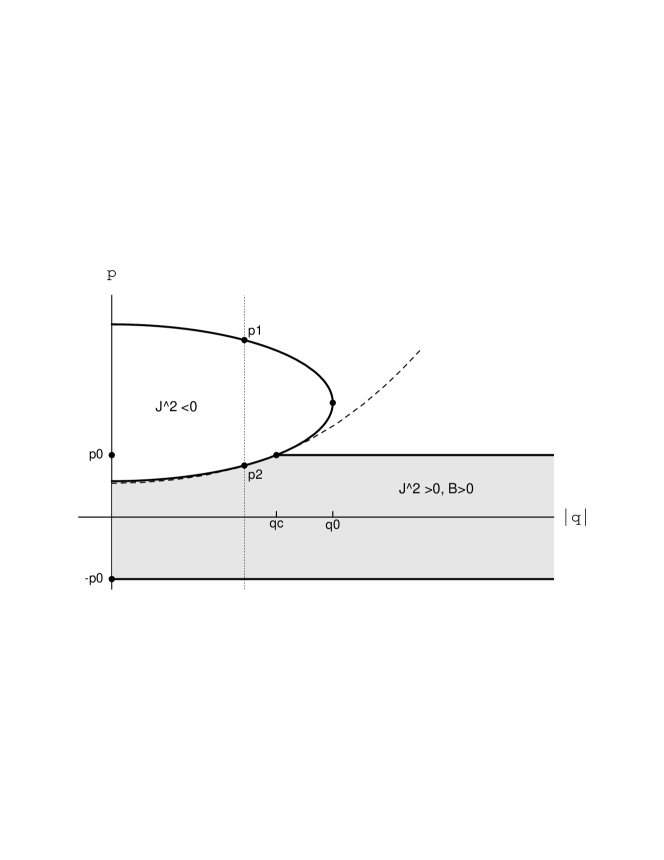
Figure 31: The $(|q|,p)$ diagram for $\Lambda_{e}>0$ and attractive charges under the condition $H\geq\sqrt{\kappa^{2}m^{2}/2\Lambda_{e}+4m^{2}}$. The dashed line represents ${\cal J}_{\Lambda}-B=0$

Figure 32: The $r(\tau)$ plots for the categories (i)-(iii) for the parameters $H_{0}=3,m=1$ and $\Lambda_{e}=1$.

6.4 $\Lambda_{e}>0$ and repulsive charges

In this case, since the cosmological repulsion is commensurate with electromagnetic repulsion, classification of the motion is analogous to that of repulsive charges with $\Lambda_{e}=0$ in sub-section 5.2. Under the condition $H<\sqrt{\kappa^{2}m^{2}/2\Lambda_{e}+4m^{2}}$ the $(|q|,p)$ diagram is given by Fig.33 which has the same pattern as Fig.10. The physical region is classified into two categories:
(i) $|q|<q_{c}$ : both bounded and unbounded motions,
(ii) $q_{c}\leq|q|$ : unbounded motion.
The trajectories of the motion for the category (ii) are divided into two cases of $q_{c}\leq|q|\leq q_{d}$ and $q_{d}<|q|$. The phase space trajectories and $r(\tau)$ plots for $|q|<q_{c}$ are analogous to those in Fig.11 and 12. For a larger $H$ of $H\geq\sqrt{\kappa^{2}m^{2}/2\Lambda_{e}+4m^{2}}$ the motion is always unbounded as inferred from the diagram of Fig.34.

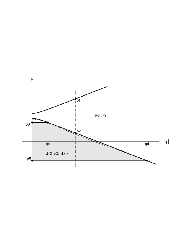
Figure 33: The $(|q|,p)$ diagram for $\Lambda_{e}>0$ and repulsive charges under the condition $H<\sqrt{\kappa^{2}m^{2}/2\Lambda_{e}+4m^{2}}$. The dashed line represents ${\cal J}_{\Lambda}-B=0$

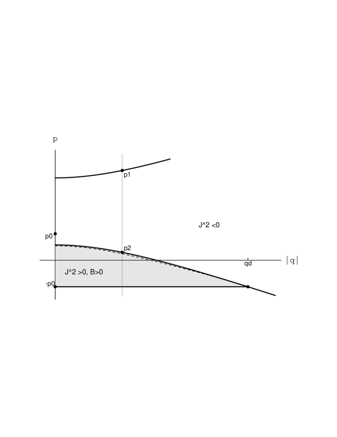
Figure 34: The $(|q|,p)$ diagram for $\Lambda_{e}>0$ and repulsive charges under the condition $H\geq\sqrt{\kappa^{2}m^{2}/2\Lambda_{e}+4m^{2}}$. The dashed line represents ${\cal J}_{\Lambda}-B=0$

7 MOTION OF UNEQUAL MASSES

What time variable is adequate for the analysis of the motion of the two particles with unequal masses? The proper time (83) of each particle is different as

$$d\tau_{1} = dt\;\frac{16YK_{0}K_{1}m_{1}}{JKM_{1}\sqrt{p^{2}+m_{1}^{2}}}\;,$$

$$d\tau_{2} = dt\;\frac{16YK_{0}K_{2}m_{2}}{JKM_{2}\sqrt{p^{2}+m_{2}^{2}}}\;,$$

where $K\equiv K_{+}=K_{-}$ and $Y\equiv Y_{+}=Y_{-}$. As with our analysis of the electrically neutral case [8], we propose using

$$d\tilde{\tau}\equiv dt\;\frac{16YK_{0}}{JK}\left(\frac{K_{1}K_{2}m_{1}m_{2}}{M_{1}M_{2}\sqrt{p^{2}+m_{1}^{2}}\sqrt{p^{2}+m_{1}^{2}}}\right)^{1/2}\;,$$ (118)

which is symmetric with respect to $1\leftrightarrow 2$ and reduces to the proper time (84) when $m_{1}=m_{2}$.

In terms of this variable the canonical equations are expressed as

$$\frac{dp}{d\tilde{\tau}} = -\frac{1}{4\kappa}\left(\frac{K_{1}K_{2}M_{1}M_{2}\sqrt{p^{2}+m_{1}^{2}}\sqrt{p^{2}+m_{2}^{2}}}{m_{1}m_{2}}\right)^{1/2}\;,$$ (119)

$$\frac{dz_{i}}{d\tilde{\tau}} = (-1)^{i+1}\left(\frac{M_{1}M_{2}\sqrt{p^{2}+m_{1}^{2}}\sqrt{p^{2}+m_{2}^{2}}}{K_{1}K_{2}m_{1}m_{2}}\right)^{1/2}\left\{\frac{\epsilon J}{16K_{0}}+\frac{K_{i}}{M_{i}}\left(\frac{p}{\sqrt{p^{2}+m_{i}^{2}}}-\epsilon\frac{Y}{K}\right)\right\}\;,$$

$$\frac{dr}{d\tilde{\tau}} = \left(\frac{M_{1}M_{2}\sqrt{p^{2}+m_{1}^{2}}\sqrt{p^{2}+m_{2}^{2}}}{K_{1}K_{2}m_{1}m_{2}}\right)^{1/2}$$ (121)

$$\makebox[30.00005pt]{}\times\left\{\frac{\epsilon J}{8K_{0}}+\frac{K_{1}}{M_{1}}\left(\frac{p}{\sqrt{p^{2}+m_{1}^{2}}}-\epsilon\frac{Y}{K}\right)+\frac{K_{2}}{M_{2}}\left(\frac{p}{\sqrt{p^{2}+m_{2}^{2}}}-\epsilon\frac{Y}{K}\right)\right\}\;.$$

Note that $r$ still describes the proper distance between the particles at any fixed instant.

Unlike the equal mass case, the integration $\int dp(K_{1}K_{2}M_{1}M_{2}\sqrt{p^{2}+m_{1}^{2}}\sqrt{p^{2}+m_{2}^{2}}\;)^{-1/2}$ can not be performed within the framework of elementary calculus. We resort to numerical calculation for solving above equations.

As in Sec.VI we analyze the motions by plotting $r(\tau)$ in four combinations of the signs of $\Lambda_{e}$ and the charges. In the case of a negative cosmological constant and attractive charges, the $r(\tau)$ plots are shown in Fig.35 for various mass ratios $m_{1}/m_{2}$ in the fixed $H_{0}=10,m_{2}=1,\Lambda_{e}=-1$ and $|q|=1$. When the mass ratio gets larger than unity (the case of $m_{1}=m_{2}=1$), the gravitational attraction is stronger and the proper distance between particles as well as the period becomes shorter. As the mass ratio gets smaller gravity becomes weak; however for quite small mass ratios the attractive effect due to the cosmological constant prevails and the period changes to being short again. The effect of the cosmological constant is seen by changing $|q|$ small but preserving the values of other parameters. Fig.36 shows the $r(\tau)$ plots for $|q|=0.1$. While both the proper distance and the period becomes large as a whole, the double peak structures appear for a small mass ratio.

Figure 35: $r(\tau)$ plots for the different values of the mass ratio $m_{1}/m_{2}$ for $H_{0}=10,m_{2}=1,\Lambda_{e}=-1$ and $e_{1}=-e_{2}=|q|=1$.

Figure 36: $r(\tau)$ plots for the same values of the parameters but $e_{1}=-e_{2}=|q|=0.1$.

In the case of $\Lambda_{e}<0$ and repulsive charges unbounded trajectories appear as $|q|$ increases. An example is shown in Fig.37, in which $r(\tau)$ for a small mass ratio $m_{1}/m_{2}=0.1$ becomes unbounded because the repulsive force between charges exceeds the weak gravity and the $\Lambda$ force.

Figure 37: $r(\tau)$ plots for different values of the mass ratio $m_{1}/m_{2}$ for $H_{0}=10,m_{2}=1,\Lambda_{e}=-1$ and $e_{1}=e_{2}=|q|=0.6$.

In the case of $\Lambda_{e}>0$ and attractive charges, as we analyzed in Sec.VI the trajectory changes from unbounded to bounded as $|q|$ increases. In Fig.38 we plot $r(\tau)$ for various $m_{1}/m_{2}$ in the fixed $H_{0}=10,m_{2}=1,\Lambda_{e}=0.1$ and $|q|=0.1$, from which the strong repulsive effect of a positive $\Lambda_{e}$ is perceived. The motions for the case of $\Lambda_{e}>0$ and the repulsive charges are mostly unbounded except for the case of the large masses.

Figure 38: $r(\tau)$ plots for the different values of the mass ratio $m_{1}/m_{2}$ for $H_{0}=10,m_{2}=1,\Lambda_{e}=0.1$ and $e_{1}=-e_{2}=|q|=0.1$.

8 STATIC BALANCE IN (1+1) DIMENSIONS

In this section we treat the problem of static balance in (1+1) dimensions. This problem originated in attempts to find the exact solution of the $N(N\geq 2)$ body system in Einstein’s theory of general relativity [12]. In $(3+1)$ dimensions gravitational radiation carries away energy from a system of particles, and so exact solutions have so far been unobtainable. One simple way to search an exact solution for $N\geq 2$ is to balance the gravitational attraction with some extra repulsive force, a natural candidate of which is the electric force. The first trial was achieved by Majumdar [13] and Papapetrou [14] for $N=2$ and afterwards it was generalized to $N$ bodies on a line [15]. Their condition for balance is

$$e_{i}=\pm\sqrt{4\pi G}\;m_{i}\;,$$ (122)

and is much more strict than the corresponding condition in Newtonian theory

$$Gm_{1}m_{2}-\frac{e_{1}e_{2}}{4\pi}=0\;.$$ (123)

Since then, the question has long been raised as to why the balance condition differs in the relativistic and non-relativistic cases. Some people [16] conjectured that there should be an exact solution in general relativity under the condition (123). Others [17, 18] showed in the (2nd) post-Newtonian approximation that the condition (123) is incompatible with the static balance condition in general relativity. Clearly (122) is a sufficient condition for static balance but there exists no proof that (122) is a necessary condition. On the other hand a test particle analysis [19] suggested that the condition (123) was neither necessary nor sufficient, but a separation-dependent balance position might exist in general relativity. Recently several numerical trials on the separation-dependence were reported [20, 21], but so far no one has been able -in any relativistic theory of gravity- to succeed in finding analytically an exact solution under (123) or another (separation-dependent) condition.

In (1+1) dimensions the absence of radiation makes it easy to fix the balance condition in terms of the determining equation (59). From the relation

$$\frac{\partial H}{\partial r}=-\frac{4K_{0}K_{1}K_{2}}{\kappa J}\;,$$ (124)

the balance condition $\partial H/\partial r=0$ leads to

$$K_{1}K_{2}=(2K_{0}+2K-\kappa\sqrt{p^{2}+m_{1}^{2}})(2K_{0}+2K-\kappa\sqrt{p^{2}+m_{2}^{2}})=0\;,$$ (125)

where $K\equiv K_{\pm}=\kappa X$ and $H=\frac{4}{\kappa}K$. In deriving (125) we excluded the possibility that $K_{0}=0$ because it gives an unphysical solution.

It is evident from (59) that the condition (125) means at the same time $M_{1}M_{2}=0$, namely,

$$(2K_{0}-2K+\kappa\sqrt{p^{2}+m_{1}^{2}})(2K_{0}-2K+\kappa\sqrt{p^{2}+m_{2}^{2}})=0\;,$$ (126)

The equations (125) and (126) lead to

$$4K_{0}^{2}+(2K-\kappa\sqrt{p^{2}+m_{1}^{2}})(2K-\kappa\sqrt{p^{2}+m_{2}^{2}})=0$$ (127)

and

$$K_{0}(4K-\kappa\sqrt{p^{2}+m_{1}^{2}}-\kappa\sqrt{p^{2}+m_{2}^{2}})=0\;.$$ (128)

The solution to (128) is

$$H=\sqrt{p^{2}+m_{1}^{2}}+\sqrt{p^{2}+m_{2}^{2}}$$ (129)

and the insertion of this solution into (127) leads to

$$\frac{\kappa}{2}(\sqrt{p^{2}+m_{1}^{2}}-\epsilon\tilde{p})(\sqrt{p^{2}+m_{2}^{2}}-\epsilon\tilde{p})-e_{1}e_{2}=0\;.$$ (130)

This condition is the force-balance condition and fixes the value of momentum $p=p_{c}=\mbox{const}$. Under the condition (130) the two particles move with a constant velocity. The condition (130) and the Hamiltonian (129) indicate that the full Hamiltonian must have the simple structure

$$H=\sqrt{p^{2}+m_{1}^{2}}+\sqrt{p^{2}+m_{2}^{2}}+\left\{\frac{\kappa}{2}(\sqrt{p^{2}+m_{1}^{2}}-\epsilon\tilde{p})(\sqrt{p^{2}+m_{2}^{2}}-\epsilon\tilde{p})-e_{1}e_{2}\right\}\;F(|r|,p)\;.$$ (131)

Actually, in the case of $\Lambda_{e}=0$ the $\kappa$-expansion of the Hamiltonian leads to

$$H = \sqrt{p^{2}+m_{1}^{2}}+\sqrt{p^{2}+m_{2}^{2}}-\frac{1}{2}e_{1}e_{2}\;|r|$$ (132)

$$+\frac{\kappa}{4}\left\{\sqrt{p^{2}+m_{1}^{2}}\sqrt{p^{2}+m_{2}^{2}}\;|r|-\epsilon\tilde{p}(\sqrt{p^{2}+m_{1}^{2}}+\sqrt{p^{2}+m_{2}^{2}}\;)|r|+p^{2}|r|\right.$$

$$\left.\makebox[20.00003pt]{}-\frac{1}{4}e_{1}e_{2}(\sqrt{p^{2}+m_{1}^{2}}+\sqrt{p^{2}+m_{2}^{2}}\;)r^{2}+\frac{1}{2}\epsilon e_{1}e_{2}\tilde{p}\;r^{2}+\frac{1}{24}(e_{1}e_{2})^{2}|r|^{3}\right\}$$

$$+\frac{\kappa^{2}}{4^{2}}\left\{\frac{1}{2\times 4}r^{2}(\sqrt{p^{2}+m_{1}^{2}}+\sqrt{p^{2}+m_{2}^{2}}-2\epsilon\tilde{p}-\frac{1}{2}e_{1}e_{2}|r|)^{3}\right.$$

$$\left.+\frac{1}{3\times 4^{2}}e_{1}e_{2}\;|r|^{3}(\sqrt{p^{2}+m_{1}^{2}}+\sqrt{p^{2}+m_{2}^{2}}-2\epsilon\tilde{p}-\frac{1}{2}e_{1}e_{2}|r|)^{2}\right.$$

$$\left.-\frac{1}{6\times 4^{2}}r^{2}\left[12(\sqrt{p^{2}+m_{1}^{2}}-\sqrt{p^{2}+m_{2}^{2}}\;)^{2}+(e_{1}e_{2})^{2}r^{2}\right]\right.$$

$$\left.\makebox[50.00008pt]{}\times(\sqrt{p^{2}+m_{1}^{2}}+\sqrt{p^{2}+m_{2}^{2}}-2\epsilon\tilde{p}-\frac{1}{2}e_{1}e_{2}|r|)\right.$$

$$\left.+\frac{1}{3\times 4^{2}}e_{1}e_{2}\;|r|^{3}(\sqrt{p^{2}+m_{1}^{2}}-\sqrt{p^{2}+m_{2}^{2}}\;)^{2}-\frac{1}{15\times 4^{3}}(e_{1}e_{2})^{3}|r|^{5}\right\}+{\cal{O}}(\kappa^{3})\;.$$

From (132) we get explicitly

$$F(|r|,p)=\frac{1}{2}|r|+\frac{\kappa}{2}(\sqrt{p^{2}+m_{1}^{2}}+\sqrt{p^{2}+m_{2}^{2}}-2\epsilon\tilde{p})\;r^{2}+{\cal{O}}(|r|^{3})\;.$$ (133)

The solution to the condition (130) exists only for $e_{1}e_{2}>0$;

$$p_{c}=\pm\frac{|\left(\frac{\kappa}{2}\right)^{2}m_{1}^{2}m_{2}^{2}-e_{1}^{2}e_{2}^{2}|}{\sqrt{2\kappa e_{1}e_{2}}\sqrt{(\frac{\kappa}{2}m_{1}^{2}+e_{1}e_{2})(\frac{\kappa}{2}m_{2}^{2}+e_{1}e_{2})}}\;.$$ (134)

When the particles are initially at rest $(p_{c}=0)$, the condition (130) becomes

$$\frac{\kappa}{2}m_{1}m_{2}-e_{1}e_{2}=0\;.$$ (135)

This is the condition of static balance and is identical with the condition in Newtonian theory in (1+1) dimensions. Note that in Newtonian theory (135) is the force-balance condition which includes both the static case and a uniform motion. However in the relativistic case (135) represents only the static balance condition – the condition of force-balance (130) in general depends on the momentum and allows a uniform motion in the C.I. ststem in which two particles approach or recede with the designated constant momentum (134).

The above result may seem to provide suggestive evidence that in (3+1) dimensions (123) could be a sufficient solution. However,the post- Newtonian Hamiltonian for the system of two charged bodies in (3+1) dimensions is given as

$$H = m_{1}+m_{2}+\frac{\mbox{\boldmath$p$}_{1}^{2}}{2m_{1}}+\frac{\mbox{\boldmath$p$}_{2}^{2}}{2m_{2}}-\frac{(\mbox{\boldmath$p$}_{1}^{2})^{2}}{8m_{1}^{3}}-\frac{(\mbox{\boldmath$p$}_{2}^{2})^{2}}{8m_{2}^{3}}$$ (136)

$$-\frac{Gm_{1}m_{2}}{r}\left\{1+\frac{3}{2}\left(\frac{\mbox{\boldmath$p$}_{1}^{2}}{m_{1}^{2}}+\frac{\mbox{\boldmath$p$}_{2}^{2}}{m_{2}^{2}}\right)-\frac{7}{2}\;\frac{(\mbox{\boldmath$p$}_{1}\cdot\mbox{\boldmath$p$}_{2})}{m_{1}m_{2}}-\frac{(\mbox{\boldmath$p$}_{1}\cdot\mbox{\boldmath$r$})(\mbox{\boldmath$p$}_{2}\cdot\mbox{\boldmath$r$})}{2m_{1}m_{2}r^{2}}\right\}$$

$$+\frac{e_{1}e_{2}}{4\pi r}\left\{1-\frac{(\mbox{\boldmath$p$}_{1}\cdot\mbox{\boldmath$p$}_{2})}{2m_{1}m_{2}}-\frac{(\mbox{\boldmath$p$}_{1}\cdot\mbox{\boldmath$r$})(\mbox{\boldmath$p$}_{2}\cdot\mbox{\boldmath$r$})}{2m_{1}m_{2}r^{2}}\right\}+\frac{G^{2}m_{1}m_{2}(m_{1}+m_{2})}{2r^{2}}$$

$$-\frac{G(m_{1}+m_{2})e_{1}e_{2}}{4\pi r^{2}}+\frac{G(m_{1}e_{2}^{2}+m_{2}e_{1}^{2})}{8\pi r^{2}}\;,$$

which is derived from Bażański Lagrangian [22] and also the ADM canonical formalism. The structure of the Hamiltonian (136) is rather complicated compared to (131). For example in (1+1) dimensional theory the charges appear always in a combination $e_{1}e_{2}$, while in (3+1) dimensions there is a combination of $m_{1}e_{2}^{2}+m_{2}e_{1}^{2}$ and in higher approximations more complicated combinations of mass and charge appear [18]. It is clear that the Hamiltonian (136) supports the balance condition (122) for the static case, while it does not correspond to a uniform motion. What causes this difference between (1+1) and (3+1) dimensional theories? Is it intrinsic to the dimensionality, or is there still a possibility for satisfying the balance condition (123) in (3+1) dimensions? Or is there a uniform motion in the C.I. system in (3+1) dimensions? These are interesting open problems for further investigation.

9 CONCLUSIONS

Since in (1+1) dimensions the degrees of freedom of both gravitational and electromagnetic radiation are frozen, one expects the motion of a set of $N$ charged particles in curved-spacetime with a cosmological constant to be described by a conservative Hamiltonian. And this is what we find to be the case. We began by canonically reducing the charged $N$-body action to first-order form and then for a system of two charged particles derived the determining equation of the Hamiltonian from the matching conditions. The canonical equations of motion given by the Hamiltonian can be solved exactly when they are expressed in terms of the proper time, and we have given the explicit solution. To our knowledge this is the first non-perturbative relativistic solution of this problem.

We recapitulate the main results of this paper:

(1) In (1+1) dimensions the square of the electric field plays the same role as the consmological constant and an overall constant part is incorporated into the effective cosmological constant $\Lambda_{e}\equiv\Lambda_{0}-\kappa(\sum_{a}e_{a})^{2}/4$, which induces the momentum-dependent potential in the Hamiltonian. Effectively $\Lambda_{e}>0$ acts on the particles as a repulsive potential and $\Lambda_{e}<0$ acts as an attractive potential.
(2) The theory in the case $\Lambda_{e}=0$ is a general relativistic electrodynamics which is an extension of flat space Newtonian electrodynamics. For the attractive charges the motion becomes bounded similar to $|q|=0$ case with smaller amplitude and period. For repulsive charges the electric force between two particles competes with the gravitational attractive force. For $|q|<q_{c}$ and a fixed energy not only bounded motion but also an infinite series of unbounded motions is realized. Such multiple solutions do not exist in Newtonian theory. For $|q|>q_{c}$ all motions become unbounded.
(3) The condition for static balance in (1+1) dimensional general relativistic electrodynamics is identical with the Newtonian balance condition in the flat space. This simple result contrasts strikingly with the unresolved situation in (3+1) dimensions.
(4) In spacetimes with nonzero $\Lambda_{e}$ the motions are more complicated. For a fixed total energy $H_{0}$ and $\Lambda_{e}$ the solutions are classified in terms of $(|q|,p)$ diagram in which the region of the parameters for the bounded and/or unbounded motions are depicted in terms of the curves of $p=\pm p_{0},{\cal{J}}_{\Lambda}^{2}=0$ and ${\cal{J}}_{\Lambda}-B=0$. By drawing a $q=\mbox{const}$ line on the diagram we can easily find what types of the motion are realized.
(5) For a certain range of $\Lambda_{e}<0$ and a small $|q|$ the double peak structure appears in $r(\tau)$ and the phase space trajectory, which is caused by a subtle interplay amongst the momentum-dependent $\Lambda$ potential, the gravitational and the electric potentials, and relativistic effects.
(6) For unbounded motion the mutual separation of two particles diverges at finite proper time. This is common for the cases of $\Lambda_{e}=0$ and $\Lambda_{e}\neq 0$.
(7) In the unequal mass case the basic features of the motion are the same, but a double peak structure appears more clearly than in the equal mass case.

A number of interesting questions arise from this work.  First, it would be of interest to know how the features of the motion we have found are modified as one increases the number of bodies in the system.  For neutral bodies this situation is relevant in modelling stellar systems and galactic evolution, where non-relativsitic one-dimensional self-gravitating systems are employed as tool toward understanding such dynamics.  For charged bodies the relevance is most likely in terms of the physics of the early universe, where charged black holes, strings and domain walls interact in a highly relativistic setting.  Second, it would be interesting to study the circumstances under which black hole event horizons can form – we expect this will involve investigating the regime where eq. (89) is not satisfied. A third possibility would involve generalizing our work to other (1+1) dilatonic theories of gravity. Moreover, a full quantum treatment of the problem would also be of considerable interest. We intend to turn our attention to these problems in the future.

APPENDIX A: SOLUTION OF THE METRIC TENSOR

Under the coordinate conditions (35) the field equations (27), (28), (31) and (32) become

$$\dot{\pi}+N_{0}\left\{\frac{3\kappa}{2}\pi^{2}+\frac{1}{8\kappa}(\Psi^{\prime})^{2}+\frac{1}{4}\left(V-\frac{\Lambda_{e}}{\kappa}\right)-\frac{p_{1}^{2}}{2\sqrt{p_{1}^{2}+m_{1}^{2}}}\delta(x-z_{1}(t))-\frac{p_{2}^{2}}{2\sqrt{p_{2}^{2}+m_{2}^{2}}}\delta(x-z_{2}(t))\right\}$$

$$+N_{1}\left\{\pi^{\prime}+p_{1}\delta(x-z_{1}(t))+p_{2}\delta(x-z_{2}(t))\right\}+\frac{1}{2\kappa}N^{\prime}_{0}\Psi^{\prime}+N^{\prime}_{1}\pi=0\;,$$ (137)

$$\kappa\pi N_{0}+N^{\prime}_{1}=0\;,$$ (138)

$$\partial_{1}(\frac{1}{2}N_{0}\Psi^{\prime}+N^{\prime}_{0})=0\;,$$ (139)

$$\dot{\Psi}+2\kappa N_{0}\pi-N_{1}\Psi^{\prime}=0\;\;.$$ (140)

The procedure to solve these equations is just the same as that in the case of $V=0$, which is given in the Appendix of the previous paper [8].

The solutions have the same form as those of $V=0$ when they are expressed in terms of $K_{\pm},K_{0},K_{1,2},{\cal M}_{1,2},Y_{\pm}$ and $J$. For $r=z_{1}-z_{2}>0$ the metric tensor is determined as

$$N_{0(+)}(x) = \frac{8}{J}\left(\frac{Y_{+}}{K_{+}}+\frac{Y_{-}}{K_{-}}\right)\frac{K_{0}K_{1}}{{\cal M}_{1}}\;e^{K_{+}(x-z_{1})}\;,$$

$$N_{0(0)}(x) = \frac{1}{2K_{0}J}\left(\frac{Y_{+}}{K_{+}}+\frac{Y_{-}}{K_{-}}\right)\left[(K_{1}{\cal M}_{1})^{\frac{1}{2}}e^{-\frac{1}{2}K_{0}(x-z_{1})}+(K_{2}{\cal M}_{2})^{\frac{1}{2}}e^{\frac{1}{2}K_{0}(x-z_{2})}\right]^{2}\;,$$

$$N_{0(-)}(x) = \frac{8}{J}\left(\frac{Y_{+}}{K_{+}}+\frac{Y_{-}}{K_{-}}\right)\frac{K_{0}K_{2}}{{\cal M}_{2}}\;e^{-K_{-}(x-z_{2})}\;,$$

$$N_{1(+)} = \epsilon\frac{Y_{+}}{K_{+}}\left\{\frac{8}{J}\left(\frac{Y_{+}}{K_{+}}+\frac{Y_{-}}{K_{-}}\right)\frac{K_{0}K_{1}}{{\cal M}_{1}}\;e^{K_{+}(x-z_{1})}-1\right\}\;,$$

$$N_{1(0)} = \epsilon\left\{\frac{Y_{0}}{2JK_{0}^{2}}\left(\frac{Y_{+}}{K_{+}}+\frac{Y_{-}}{K_{-}}\right)\left[K_{2}M_{2}\;e^{K_{0}(x-z_{2})}-K_{1}M_{1}\;e^{-K_{0}(x-z_{1})}\right.\right.$$

$$\makebox[50.00008pt]{}\left.\left.+2K_{0}(K_{1}K_{2}M_{1}M_{2})^{1/2}\;e^{\frac{1}{2}K_{0}(z_{1}-z_{2})}\;x\right]+D_{0}\right\}\;,$$

$$N_{1(-)} = -\epsilon\frac{Y_{-}}{K_{-}}\left\{\frac{8}{J}\left(\frac{Y_{+}}{K_{+}}+\frac{Y_{-}}{K_{-}}\right)\frac{K_{0}K_{2}}{{\cal M}_{2}}\;e^{-K_{-}(x-z_{2})}-1\right\}\;,$$

where

$$D_{0} = -\frac{1}{2}\left(\frac{Y_{+}}{K_{+}}-\frac{Y_{-}}{K_{-}}\right)+\frac{1}{2J}\left(\frac{Y_{+}}{K_{+}}+\frac{Y_{-}}{K_{-}}\right)\left\{2\left[\left(\frac{Y_{0}}{K_{0}}+\frac{Y_{+}}{K_{+}}\right)K_{1}-\left(\frac{Y_{0}}{K_{0}}+\frac{Y_{-}}{K_{-}}\right)K_{2}\right]\right.$$ (142)

$$\left.-2\left[\left(\frac{Y_{0}}{K_{0}}-\frac{Y_{+}}{K_{+}}\right)\frac{1}{{\cal M}_{1}}-\left(\frac{Y_{0}}{K_{0}}-\frac{Y_{-}}{K_{-}}\right)\frac{1}{{\cal M}_{2}}\right]K_{1}K_{2}-\frac{Y_{0}}{K_{0}}K_{1}K_{2}(z_{1}+z_{2})\right\}\;.$$

The metric tensor for $r<0$ is simply obtained by interchanging the suffix 1 and 2. With these metric tensors and the canonical equations, the field equations (137), (138) and (139) are proved to hold in a whole $x$ space.

As we showed in the previous paper, to satisfy (140) the dilaton field $\Psi$ needs an extra $x$-independent function $f(t)$, which has no effect on the dynamics of particles. After lengthy calculation Eq.(140) leads to

$$\dot{f}(t) = -\frac{d}{dt}(K_{01}z_{1}-K_{02}z_{2})+\frac{2}{J}\left(\frac{Y_{+}}{K_{+}}+\frac{Y_{-}}{K_{-}}\right)\left\{2K_{0}K_{1}\frac{p_{1}}{\sqrt{p_{1}^{2}+m_{1}^{2}}}-2K_{0}K_{2}\frac{p_{2}}{\sqrt{p_{2}^{2}+m_{2}^{2}}}\right.$$ (143)

$$\left.+\epsilon\frac{Y_{0}}{K_{0}}\left(K_{0}K_{1}+K_{0}K_{2}-\frac{K_{0}K_{1}K_{2}}{{\cal M}_{1}}-\frac{K_{0}K_{1}K_{2}}{{\cal M}_{2}}\right)+4\epsilon Y_{0}K_{0}\left(\frac{K_{1}}{{\cal M}_{1}}+\frac{K_{2}}{{\cal M}_{2}}\right)\right\}\;\;.$$

Thus $f(t)$ is uniquely determined.

APPENDIX B: LINEAR APPROXIMATION OF THE EXACT SOLUTION IN $\Lambda_{e}=0$

In this appendix we investigate how the exact solution is related to its corresponding solution in Newtonian theory. Take the tanh-type A solution, namely a periodic motion with $e_{1}e_{2}<0$ or small $e_{1}e_{2}>0$. For motion starting from $r=0$ at $\tau=\tau_{0}=0$, the relationship between the energy and the initial momentum is $H_{0}=2\sqrt{p_{0}^{2}+m^{2}}$.

In the $\kappa$ expansion, $f_{e}(\tau)$ is expressed as

$$f_{e}(\tau) = \frac{\sqrt{p_{0}^{2}+m^{2}}+\epsilon p_{0}}{m}\;e^{\frac{\epsilon\tau}{2m}e_{1}e_{2}}$$ (144)

$$-\kappa m\left[\frac{\sqrt{p_{0}^{2}+m^{2}}}{e_{1}e_{2}}\left(e^{\frac{\epsilon\tau}{2m}e_{1}e_{2}}-1\right)-(\sqrt{p_{0}^{2}+m^{2}}+\epsilon p_{0})\frac{\epsilon\tau}{4m}\;e^{\frac{\epsilon\tau}{2m}e_{1}e_{2}}\right]+{\cal O}(\kappa^{2})$$

and $p(\tau)$ is

$$p = \sqrt{p_{0}^{2}+m^{2}}\;\mbox{sinh}\frac{e_{1}e_{2}\tau}{2m}+p_{0}\;\mbox{cosh}\frac{e_{1}e_{2}\tau}{2m}$$ (145)

$$-\frac{\kappa m^{2}}{2\epsilon}\left[1+\frac{(\sqrt{p_{0}^{2}+m^{2}}-\epsilon p_{0})^{2}}{m^{2}}\;e^{-\frac{\epsilon\tau}{m}e_{1}e_{2}}\right]$$

$$\makebox[20.00003pt]{}\times\left[\frac{\sqrt{p_{0}^{2}+m^{2}}}{e_{1}e_{2}}\left(e^{\frac{\epsilon\tau}{2m}e_{1}e_{2}}-1\right)-(\sqrt{p_{0}^{2}+m^{2}}+\epsilon p_{0})\frac{\epsilon\tau}{4m}\;e^{\frac{\epsilon\tau}{2m}e_{1}e_{2}}\right]+{\cal O}(\kappa^{2})\;.$$

The trajectory $r(\tau)>0$ in the linear approximation becomes

$$r(\tau) = -\frac{4}{e_{1}e_{2}}\left[\sqrt{p_{0}^{2}+m^{2}}\left(1-\mbox{cosh}\frac{e_{1}e_{2}\tau}{2m}\right)-p_{0}\;\mbox{sinh}\frac{e_{1}e_{2}\tau}{2m}\right]$$ (146)

$$-\frac{4\kappa\epsilon}{e_{1}e_{2}}\left[\sqrt{p_{0}^{2}+m^{2}}\;\mbox{sinh}\frac{e_{1}e_{2}\tau}{2m}+p_{0}\;\mbox{cosh}\frac{e_{1}e_{2}\tau}{2m}\right]$$

$$\makebox[50.00008pt]{}\times\left[\frac{\sqrt{p_{0}^{2}+m^{2}}(\sqrt{p_{0}^{2}+m^{2}}-\epsilon p_{0})}{e_{1}e_{2}}\left(1-e^{-\frac{\epsilon\tau}{2m}e_{1}e_{2}}\right)-\frac{\epsilon m\tau}{4}\right]$$

$$-\frac{4\kappa}{e_{1}e_{2}}\left[\sqrt{p_{0}^{2}+m^{2}}\left(1-\mbox{cosh}\frac{e_{1}e_{2}\tau}{2m}\right)-p_{0}\;\mbox{sinh}\frac{e_{1}e_{2}\tau}{2m}\right]$$

$$\makebox[10.00002pt]{}\times\left\{\frac{1}{2e_{1}e_{2}}\left[\sqrt{p_{0}^{2}+m^{2}}\left(1-\epsilon\;\mbox{sinh}\frac{e_{1}e_{2}\tau}{2m}\right)-\epsilon p_{0}\;\mbox{cosh}\frac{e_{1}e_{2}\tau}{2m}\right]^{2}\right.$$

$$\makebox[50.00008pt]{}\left.-\frac{1}{6e_{1}e_{2}}\left[\sqrt{p_{0}^{2}+m^{2}}\left(1-\mbox{cosh}\frac{e_{1}e_{2}\tau}{2m}\right)-p_{0}\;\mbox{sinh}\frac{e_{1}e_{2}\tau}{2m}\right]^{2}\right\}\;\;.$$

Furthermore in the limit $\kappa\rightarrow 0$ the solution is

$$p = \sqrt{p_{0}^{2}+m^{2}}\;\mbox{sinh}\frac{e_{1}e_{2}\tau}{2m}+p_{0}\;\mbox{cosh}\frac{e_{1}e_{2}\tau}{2m}\;,$$

$$r = -\frac{4}{e_{1}e_{2}}\left[\sqrt{p_{0}^{2}+m^{2}}\left(1-\mbox{cosh}\frac{e_{1}e_{2}\tau}{2m}\right)-p_{0}\;\mbox{sinh}\frac{e_{1}e_{2}\tau}{2m}\right]\;\;.$$

We can transform it into an expression in terms of the original time coordinate $t$, by using the relation

$$t=\frac{2\sqrt{p_{0}^{2}+m^{2}}}{e_{1}e_{2}}\;\mbox{sinh}\frac{e_{1}e_{2}\tau}{2m}+\frac{2p_{0}}{e_{1}e_{2}}\;\left(\mbox{cosh}\frac{e_{1}e_{2}\tau}{2m}-1\right)$$ (148)

which is obtained by integrating (84). Then

$$p(t) = p_{0}+\frac{e_{1}e_{2}}{2}t\;,$$ (149)

$$r(t) = \frac{4}{e_{1}e_{2}}\left\{\sqrt{(p_{0}+\frac{e_{1}e_{2}}{2}t)^{2}+m^{2}}-\sqrt{p_{0}^{2}+m^{2}}\right\}\;\;.$$ (150)

This solution is identical with that derived from the Hamiltonian for flat-space electrodynamics in (1+1) dimensions: $H=2\sqrt{p^{2}+m^{2}}-e_{1}e_{2}|r|/2$. The same solution can be applied to the system of arbitrary charges as far as $H_{0}\geq 2m$.

On the other hand, for the repulsive charges $(e_{1}e_{2}>0)$ there exists the solution for $H_{0}<2m$, which denotes an unbounded motion and is given by

$$p(t) = \frac{e_{1}e_{2}}{2}t\;,$$ (151)

$$r(t) = \frac{4}{e_{1}e_{2}}\;\left\{\sqrt{\frac{(e_{1}e_{2})^{2}}{4}t^{2}+m^{2}}-\frac{H_{0}}{2}\right\}\;.$$ (152)

This solution is also derived from the tan-type A solution in the limit $\kappa\rightarrow 0$.

Another limit of the solution (146) is to take $e_{a}\rightarrow 0$, which leads to

$$r(\tau)=\frac{2p_{0}}{m}\;\tau-\kappa\frac{\sqrt{p_{0}^{2}+m^{2}}}{4}\;\tau^{2}\;\;.$$ (153)

In the non-relativistic approximation (keeping the terms to the lowest order of $p_{0}/m$) we get the solution for the motion in Newtonian gravity in (1+1) dimensions:

$$r(t)=\frac{2p_{0}}{m}\;t-\frac{\kappa m}{4}\;t^{2}\;\;.$$ (154)

APPENDIX C: CAUSAL RELATIONSHIPS BETWEEN PARTICLES

One of the striking features we found in the analysis of the two body motion is that in the repulsive trajectories $N_{1},N_{2},A_{n}$ and $B_{n}$ the particles reach the asymptotic regime ($r\rightarrow\pm\infty,p=\mbox{finite}$) at some finite proper time $\tau_{\infty}$. For example for $N_{1}$ trajectory it is

$$\tau_{\infty}=\frac{4}{\kappa m\sqrt{\gamma_{m}}}\mbox{log}\left(\frac{H(1+\sqrt{\gamma_{m}})-\left\{p_{+}+\sqrt{p_{+}^{2}+m^{2}}\right\}(\sqrt{\gamma_{m}}+\gamma_{e})}{\left[H(1+\sqrt{\gamma_{m}})+\left\{p_{+}+\sqrt{p_{+}^{2}+m^{2}}\right\}(\sqrt{\gamma_{m}}-\gamma_{e})\right]\eta}\right)$$ (155)

with $p_{+}=\frac{1}{2\kappa}\left\{\sqrt{\kappa^{2}H^{2}+8\Lambda_{e}}+\sqrt{8\Lambda_{e}+8e_{1}e_{2}}\right\}$.

We can understand this feature in a simple flat-space model. Consider the 2-velocity

$$u^{\mu}=(f(\sigma\tau),\sqrt{f^{2}(\sigma\tau)-1})\quad\mbox{with}\quad d\tau^{2}=dt^{2}-dx^{2}\;,$$ (156)

where $f(\sigma\tau)$ is some function. This 2-velocity means

$$\frac{dx}{dt}=\frac{\sqrt{f^{2}-1}}{f}\;,$$ (157)

and leads to the 2-acceleration

$$a^{\mu}=\frac{du^{\mu}}{d\tau}=f^{\prime}\sigma(1,\frac{f}{\sqrt{f^{2}(\sigma\tau)-1}})\;,$$ (158)

where $f^{\prime}=df(\tau)/d\tau$. There exist functions $f$ such that $f\rightarrow\infty$ as $\tau\rightarrow\tau_{\infty}$, $\tau_{\infty}$ being finite; the particle thus becomes lightlike in a finite amount of proper time, but an infinite amount of coordinate time $t=\int_{\tau_{i}}^{\tau}d\tau f(\sigma\tau)$. An example would be $f=\sec(\sigma\tau)$. The acceleration is not constant, but increases as a function of proper time, diverging at $\tau=\tau_{\infty}\equiv\frac{\pi}{2\sigma}$. This is the situation we encounter for the unbounded motions of two charged particles (or of two neutral particles with sufficiently large positive cosmological constant).

To see the causal relationships between particles and the space-time structure we try to pursue the path of light signal emitted from particle 2 in the metric given in Appendix A. The path $x(t)$ of the light is governed by $d\tau=0$, which reads

$$\left(\frac{dx}{dt}\right)^{2}+2N_{1}\frac{dx}{dt}-(N_{0}^{2}-N_{1}^{2})=0\;.$$ (159)

The equation of the light signal emitted inward (directed to particle 1) is

$$\frac{dx}{dt}=N_{0}(x(t),z_{1}(t),z_{2}(t),p(t))-N_{1}(x(t),z_{1}(t),z_{2}(t),p(t))\;,$$ (160)

and the light emitted outward is described by

$$\frac{dx}{dt}=-N_{0}(x(t),z_{1}(t),z_{2}(t),p(t))-N_{1}(x(t),z_{1}(t),z_{2}(t),p(t))\;.$$ (161)

Let’s take first a typical bounded motion in the case of $\Lambda_{e}=0$ and the attractive charges for the parameters of $H_{0}=3,m=1$ and $q=1$. In Fig.39 the trajectories of light signals emitted from particle 2 at various times $T$ are plotted. The two particles are always in causal contact, because the inward light signal from particle 2 reaches particle 1. We see one striking feature for the case of $\Lambda_{e}=0$, namely that the outward light pulse has a constant velocity $c$, since the equations (160) and (161) become $dx/dt=\pm 1$, where the plus and the minus signs correspond to the light emitted outward from the particle 1 and 2, respectively.

Figure 39: The trajectories of light signals emitted from the particle 2 for the case of $\Lambda_{e}=0$.

Next we look into the effect of the cosmological constant on the path of the light signal. Fig.40 shows the trajecories of light for the case of a negative cosmological constant $\Lambda_{e}=-1$ and the same values of the parameters $H_{0},m$ and $q$. The outward light behaves as if it is subjected to a repulsive force, in significant contrast to the particles’ trajectories on which the cosmological constant acts effectively as an attractive force as we analyzed in Sec.VI. On the other hand, while the positive cosmological constant causes a repulsive force between particles, the outward light behaves as if it undergoes an attractive force and approaches a kind of horizon given by the line $N_{0}(x,z_{1}(t),z_{2}(t),p(t))\pm N_{1}(x,z_{1}(t),z_{2}(t),p(t))=0$ which is shown in Fig.41 as a narrow solid line for the case of $\Lambda_{e}=0.5$.

Figure 40: The trajectories of light signals emitted from the particle 2 for the case of $\Lambda_{e}=-1$.

Figure 41: The trajectories of light signals emitted from the particle 2 for the case of $\Lambda_{e}=0.5$. The narrow solid line denotes $N_{0}(x,z_{1}(t),z_{2}(t),p(t))+N_{1}(x,z_{1}(t),z_{2}(t),p(t))=0$.

When the cosmological constant exceeds a critical value, the particles’ motion becomes unbounded and the light signals emitted from the particle 2 exhibit new characteristics as shown in Fig.42 for the case of $\Lambda_{e}=2.5$. For small $T(T<0.9)$, the particles are in causal contact (the inward dotted curve), but for $T\approx 0.9$ the signal just barely catches up with particle 1, which is almost in light-like motion (the inward dashed curve). For $T=2$ the inward world line $x(t)$ is parallel to $z_{1}(t)$ at large $t$ and in the outward direction it goes nearly on the same trajectory with the particle 2. For large $T$ ($T>2$) the particles are out of causal contact with each other : a light ray sent from particle 2 toward particle 1 receives a strong repulsive effect and ultimately reverses direction, following behind particle 2.

Figure 42: The trajectories of light signals emitted from the particle 2 for the case of $\Lambda_{e}=2.5$.

Acknowledgements

This work was supported in part by the Natural Sciences and Engineering Research Council of Canada.

References

[1] R.B. Mann, Found. Phys. Lett. 4 (1991) 425; R.B. Mann,
Gen. Rel. Grav. 24 (1992) 433.