Removing Line Interference from Gravitational Wave Interferometer Data

Abstract

We describe a procedure to identify and remove a class of interference lines from gravitational wave interferometer data. We illustrate the usefulness of this technique applying it to prototype interferometer data and removing all those lines corresponding to the external electricity main supply and related features.

1. Introduction

In the measured noise spectrum of the different gravitational wave interferometer prototypes, we observe peaks due external interference [1,2]. The most numerous are powerline frequency harmonics. We have shown how to model and remove these lines very effectively using a technique we call coherent line removal (clr) [3]. In addition to those lines appearing at multiples of 50 (or 60) Hz, there are other interference lines whose frequencies change in step with the supply frequency, but not at the harmonic frequencies. The easiest way to detect their presence is by studying in detail the spectrogram (see figure 1). These lines, although they are not as powerful as the harmonics, are spread over the whole spectrum. From a data analysis point of view, we try to develop a technique able to remove this interference while producing a minimum disturbance to the underlying noise background [4].

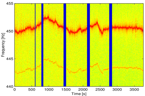
Fig. 1.: Zoom of the spectrogram of the prototype data. The line near 450 Hz corresponds to the 9th harmonic of the external electricity supply. The weaker line near 443 Hz is one example of the many lines present in the spectrum that have a similar time-frequency evolution to that of the harmonics of 50 Hz.

In this paper, we illustrate the usefulness of these techniques by applying them to the data produced by the Glasgow laser interferometer in March 1996. As a result the interference is attenuated or eliminated by cancellation in the time domain and the power spectrum appears completely clean allowing the detection of signals that were buried in the interference. Therefore, these new methods appear to be good news as far as searching for continuous waves is concerned. The removal reduces the level of non-Gaussian noise, improving the sensitivity of the detector to short bursts of gravitational waves as well.

2. Line removal

clr is an algorithm able to remove interference present in the data while preserving the stochastic detector noise. clr works when the interference is present in many harmonics, as long as they remain coherent with one another. It can remove the external interference without removing any ‘single line’ signal buried by the harmonics. The algorithm works even when the interference frequency changes. clr can be used to remove all harmonics of periodic or broad-band signals (e.g., those which change frequency in time), even when there is no external reference source. It assumes that the interference has the form

$$y(t)=\sum_{n}a_{n}m(t)^{n}+\left(a_{n}m(t)^{n}\right)^{*}\ ,$$ (1)

where $a_{n}$ are complex amplitudes and $m(t)$ is a nearly monochromatic function near a frequency $f_{0}$. The idea is to use the information in the different harmonics of the interference to construct a function $M(t)$ that is as close a replica as possible of $m(t)$ and then construct a function close to $y(t)$ which is subtracted from the output of the system cancelling the interference. The key is that real gravitational wave signals will not be present with multiple harmonics and that $M(t)$ is constructed from many frequency bands with independent noise. Hence, clr will little affect the statistics of the noise in any one band and any gravitational wave signal masked by the interference can be recovered without any disturbance.

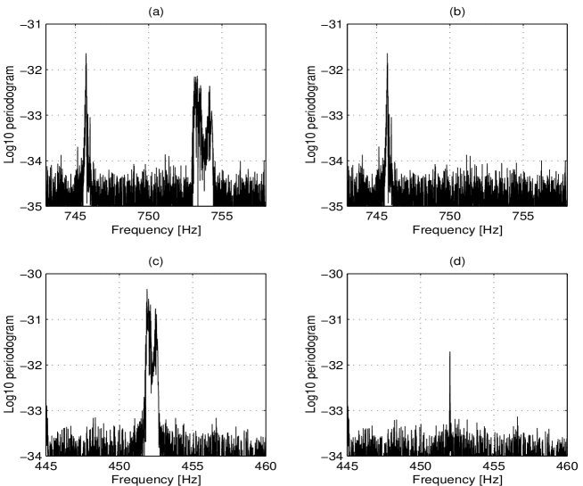
Fig. 2.: Decimal logarithm of the periodogram of $2^{19}$ points of the prototype data. (a) One of the harmonics near 754 Hz. (b) The same data after the removal of the interference using clr. (c) The same experimental data with an artificial signal added at 452 Hz. (d) The data in (c) after the removal of the interference, revealing that the signal remains detectable.

In figure 2, we show the performance of clr on two minutes of data. We can see how clr leaves the spectrum clean of the interference and keeps the intrinsic detector noise.

For the non-harmonic lines, after examining them in detail and rejecting the possibility of the beats, we assume a noninteger harmonic of the supply

$$y(t)=\alpha(t)M(t)^{q}\ ,$$ (2)

where $\alpha(t)$ is a slowly varying complex amplitude, $M(t)$ is a reference wave form corresponding the fundamental harmonic (that can be obtained using clr), but $q$ is a real number, not only an integer as in the case of the harmonics (and it can also drift in time $q(t)=q_{0}+\delta q(t)$, where $\delta q(t)$ is small in comparison to $q_{0}$). See [4] for details. The justification for this model is simply the success we have in removing the interference as we show in figures 3 and 4.

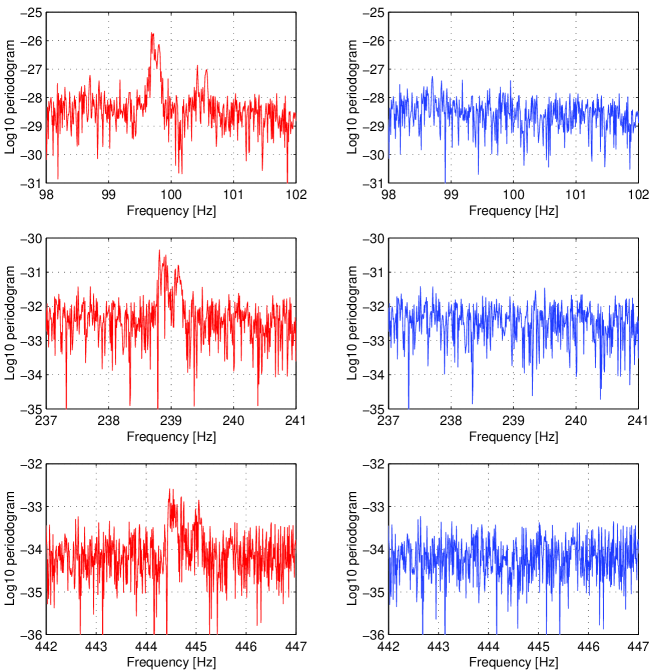
Fig. 3.: Decimal logarithm of the periodogram of $2^{19}$ points of the prototype data. (Left) Details of the lines near 99.5, 100.5, 239 and 445 Hz. (Right) The same data after removing the electrical interference.

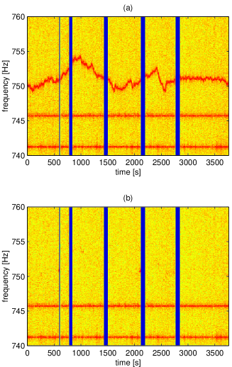
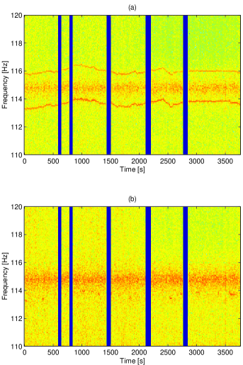
Fig. 4.: Comparison of a zoom of the spectrogram. (Left) (a) is obtained from the prototype data. We can observe the wandering of the incoming electrical signal. The other two remaining lines at constant frequency correspond to violin modes. (b) The same spectrogram as in (a) after applying clr, showing how the electrical interference is completely removed. (Right) (a) The prototype data with two anomalous lines near 114 and 116 Hz. (b) The same spectrogram as in (a) after removing the interference.

In figure 4, we compare zooms of the spectrogram. There we can see the performance of both algorithms on the whole data stream, showing how the lines due to electrical interference in the initial data are removed.

We are interested in studying possible side effects of the line removal on the statistics of the noise in the time domain. For the Glasgow data, the standard deviation value is around 1.50 Volts. After the line removal, the standard deviation is reduced to 1.05 Volts. This indicates that a huge amount of power has been removed. Further analysis reveals that values of skewness and kurtosis are getting closer to zero after the line removal. Values of skewness and kurtosis near zero suggest a Gaussian nature. Therefore, we are interested in studying the possible reduction of the level of non-Gaussian noise. To this end, we take a piece of data and we study their histogram, calculating the number of events that lie between different equal intervals. If we plot the logarithm of the number of events versus $(x-\mu)^{2}$, where $x$ is the central position of the interval and $\mu$ is the mean, in case of a Gaussian distribution, all points should fit on a straight line of slope $-1/2\sigma^{2}$, where $\sigma$ is the standard deviation. We observe that this is not the case. See figure 5. Although, both distributions seem to have a linear regime, they present a break and then a very heavy tail. The two distributions are very different. This is mainly due to the change of the standard deviation. We can zoom the ‘linear’ regime and change the scale in the abscissa to $(x-\mu)^{2}/(2\sigma^{2})$. Then, any Gaussian distribution should fit into a straight line of slope -1. We observe that after removing the interference, it follows a Gaussian distribution quite well up to $4\sigma$. The original Glasgow data does not fit a straight line anywhere.

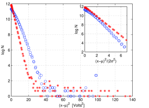
Fig. 5.: Comparison of the logarithm plot of the histogram for $3.2\times 2^{19}$ points as a function of $(x-\mu)^{2}$. The circles correspond to the Glasgow data and the stars to the same data after removing the electrical interference. In the right-hand corner, there is zoom of the original figure, but rescaled so that the abscissa corresponds to $(x-\mu)^{2}/2\sigma^{2}$.

We have also applied two statistical tests to the data: the chi-square test that measures the discrepancies between binned distributions, and the one-dimensional Kolmogorov-Smirnov test that measures the differences between cumulative distributions of a continuous data. In both tests, the significance probability increased after removing the electrical interference, showing that these procedures suppress some non-Gaussian noise, although, generally speaking, the distribution was still non-Gaussian in character. See [3] for details.

3. References

1.  Abramovici A. et al. 1996, Phys. Lett. A 218, 157

2. Robertson D.I. et al.  1995, Rev. Sci. Instrum. 66, 4447

3. Sintes A. M., Schutz B.F. 1998, Phys. Rev. D, 58, 122003

4. Sintes A. M., Schutz B.F. 1999, Phys. Rev. D, 60, 062001