Notes on causal differencing in ADM/CADM formulations: a 1D comparison

Abstract

Causal differencing has shown to be one of the promising and successful approaches towards excising curvature singularities from numerical simulations of black hole spacetimes. So far it has only been actively implemented in the ADM and Einstein-Bianchi 3+1 formulations of the Einstein equations. Recently, an approach closely related to the ADM one, commonly referred to as as “conformal ADM” (CADM) has shown excellent results when modeling waves on flat spacetimes and black hole spacetimes where singularity avoiding slices are used to deal with the singularity. In these cases, the use of CADM has yielded longer evolutions and better outer boundary dependence than those obtained with the ADM one. If this success translates to the case where excision is implemented, then the CADM formulation will likely be a prime candidate for modeling generic black hole spacetimes. In the present work we investigate the applicability of causal differencing to CADM, presenting the equations in a convenient way for such a goal and compare its application with the ADM approach in 1D.

I Introduction

One of the goals of numerical relativity that has proven to be elusive (using a 3+1 splitting of the Einstein equations) has been that of modeling a generic single black hole long periods of time. Present single black hole simulations in 3D have not yet been shown to be generically stable. There are limited instances of stability based on the outer boundary choice and placement[1, 2]. Most simulations run just beyond a few hundreds $M$ based on outer boundary placement and binary black hole simulations run for about $20-50M$ before the codes either crash or the entire grid is inside the event horizon. In some cases, the reason of the crash is well understood. For instance, the use of singularity avoiding slices lead to the presence of steep gradients which eventually can no longer be handled by the codes. A solution to this problem is to “excise” the singularity from the computational domain[3]. Unfortunately, in most cases, it is not clear what the main reasons behind the crash are and consequently addressing the problem becomes cumbersome. In attempting to deal with this issue there are several possible avenues to either remove or provide an understanding of the source of problems. These avenues can be divided in the following way:

1. Choice of formulation of Einstein equations;

2. Choice of gauge;

3. Numerical implementations.

Avenue (1) is motivated by the difficulties encountered in achieving long term evolutions with the ADM formulation, which historically has been the main tool in Numerical Relativity. Several formulations exist in the literature that exhibit properties like hyperbolicity[4], the equations are expressed in a flux conservative form[5] and/or try to separate transverse modes[6, 7, 8]. Avenue (2) is based on the fact that, in principle, a coordinate system could be chosen such that the fields vary slowly in time; hence, the simulations would be better behaved. Conditions to achieve such coordinates have been presented in the literature[9]. Lastly, avenue (3) highlights the need for a more profound understanding of the numerical implementation of the evolution equations. Algorithms specifically tailored to deal with the equations under study could pave the way to better behaved simulations (for instance, compare with the implementations that deal with the fluid equations and their ‘historical evolution’ from crude implementations in early simulations to high resolution shock capturing schemes in present state of the art codes).

Our present work focuses primarily on avenue (1); although avenues (2) and (3) also play a role since notable improvements are achieved with specific gauge choices and the use of causal differencing algorithms. We compare results obtained from the use of black hole excision with two related forms of the standard ADM 3+1 equations; focusing on the use of the CADM system with excision techniques in spherical symmetry.

The main motivation behind the comparison with the conformal ADM is the report by many groups that robust implementations have been achieved in linearized gravity, gravitational wave spacetimes, systems containing matter, etc[10, 7, 11]. However, so far, it has only been used to model black hole spacetimes using singularity avoiding slices[12]. As it is widely accepted, these types of slicings are useful when the desired simulation time is rather short. In order to model black hole spacetimes for long periods of time, singularity excision must be employed. To study the feasibility of excision in this formulation and to analyze its advantages and disadvantages with respect to the traditional ADM formulation (where excision techniques have been used for several years already[13, 14]), we present a $1D$ study and compare results obtained with both approaches. We start with a brief review of the formulations in section II. In section III, we rewrite the system of equations in a way convenient for causal differencing and describe how this techniques is implemented. In section IV we compare simulations of a Schwarzschild black hole and show how the ADM formulation yields longer term evolution unless the trace of the extrinsic curvature is frozen in time, in which case CADM yields better behaved evolutions than the ADM formulation, we also show how causal differencing indeed gives the expected results in terms of stability. We conclude in section V with a brief discussion.

II Formulation

The standard ADM equations, in the form most commonly used in numerical relativity, are[15]:

$$\frac{d}{dt}\;\gamma_{ij} = -2\alpha K_{ij},$$ (2)

$$\frac{d}{dt}\;K_{ij} = -D_{i}D_{j}\alpha+\alpha\left(\rule{0.0pt}{11.38109pt}R_{ij}+KK_{ij}\right.$$ (4)

$$\left.-2K_{ik}K^{k}{}_{j}-{}^{(4)}R_{ij}\right),$$

with

$$\frac{d}{dt}=\partial_{t}-\cal{L}_{\beta}\,,$$ (5)

where $\cal{L}_{\beta}$ is the Lie derivative along the shift vector $\beta^{i}$; $R_{ij}$ is the Ricci tensor and $D_{i}$ the covariant derivative associated with the three-dimensional metric $\gamma_{ij}$.

The conformal ADM equations [6, 7] are obtained from the ADM ones by (I) making use of a conformal decomposition of the three-metric as

$$\tilde{\gamma}_{ij}=e^{-4\phi}\gamma_{ij}\,\,\,\mbox{with}\,\,\,e^{4\phi}=\gamma^{1/3}\equiv\det(\gamma_{ij})^{1/3}\,;$$ (6)

(hence $det(\tilde{\gamma})=1$); (II) decomposing the extrinsic curvature into its trace and trace-free components. The trace-free part of the extrinsic curvature $K_{ij}$, defined by

$$A_{ij}=K_{ij}-\frac{1}{3}\gamma_{ij}K,$$ (7)

and $K=\gamma^{ij}K_{ij}$ is the trace of the extrinsic curvature and (III) further conformally decomposing $A_{ij}$ as:

$$\tilde{A}_{ij}=e^{-4\phi}A_{ij}\,.$$ (8)

In terms of these variables, Einstein equations in vacuum are [6, 7]

$$\frac{d}{dt}\tilde{\gamma}_{ij} = -2\alpha\tilde{A}_{ij},$$ (10)

$$\frac{d}{dt}\phi = -\frac{1}{6}\alpha K\,,$$ (11)

$$\frac{d}{dt}K = -\gamma^{ij}D_{i}D_{j}\alpha+\alpha\left[\tilde{A}_{ij}\tilde{A}^{ij}+\frac{1}{3}K^{2}\right],$$ (12)

$$\frac{d}{dt}\tilde{A}_{ij} = e^{-4\phi}\left[-D_{i}D_{j}\alpha+\alpha R_{ij}\right]^{TF}\noindent$$ (14)

$$+\alpha\left(K\tilde{A}_{ij}-2\tilde{A}_{il}\tilde{A}_{j}^{l}\right),$$

where the Hamiltonian constraint was used to eliminate the Ricci scalar in equation (12). Note that with the conformal decomposition of the three–metric, the Ricci tensor now has two pieces, which are written as

$$R_{ij}=\tilde{R}_{ij}+R^{\phi}_{ij}.$$ (15)

The “conformal-factor” part $R^{\phi}_{ij}$ is given directly by straightforward computation of derivatives of $\phi$:

$$R^{\phi}_{ij} = -2\tilde{D}_{i}\tilde{D}_{j}\phi-2\tilde{\gamma}_{ij}\tilde{D}^{l}\tilde{D}_{l}\phi\noindent$$ (17)

$$+4\tilde{D}_{i}\phi\;\tilde{D}_{j}\phi-4\tilde{\gamma}_{ij}\tilde{D}^{l}\phi\;\tilde{D}_{l}\phi,$$

while the “conformal” part $\tilde{R}_{ij}$ can be computed in the standard way from the conformal three–metric $\tilde{\gamma}_{ij}$.

To this point, the equations have been written by a trivial algebraic manipulation of the ADM equations in terms of the new variables. The non-trivial part comes into play by introducing what Ref. [7] calls the “conformal connection functions”:

$$\tilde{\Gamma}^{i}:=\tilde{\gamma}^{jk}\tilde{\Gamma}^{i}_{jk}=-\tilde{\gamma}^{ij}_{~{}~{},j},$$ (18)

where the last equality holds since the determinant of the conformal three–metric $\tilde{\gamma}$ is unity. Using the conformal connection functions, the Ricci tensor is written as:

$$\tilde{R}_{ij} = -\frac{1}{2}\tilde{\gamma}^{lm}\tilde{\gamma}_{ij,lm}+\tilde{\gamma}_{k(i}\partial_{j)}\tilde{\Gamma}^{k}+\tilde{\Gamma}^{k}\tilde{\partial}_{(j}\tilde{\gamma}_{i)k}$$ (20)

$$-\tilde{\gamma}^{kl}_{(,j}\tilde{\gamma}_{i)l,k}-\tilde{\Gamma}^{l}\tilde{\Gamma}_{ijl}-\Gamma^{l}_{kj}\Gamma^{k}_{li}\,.$$

Where $\tilde{\Gamma}^{i}$ are to be considered independent variables whose evolution equations are obtained by a simple commutation of derivatives.

$$\frac{\partial}{\partial t}\tilde{\Gamma}^{i} = -\frac{\partial}{\partial x^{j}}\Big{(}2\alpha\tilde{A}^{ij}-2\tilde{\gamma}^{m(j}\beta^{i)}_{~{},m}\noindent$$ (22)

$$+\frac{2}{3}\tilde{\gamma}^{ij}\beta^{l}_{~{},l}+\beta^{l}\tilde{\gamma}^{ij}_{~{}~{},l}\Big{)}.$$

As proposed in Ref. [7] the divergence of $\tilde{A}^{ij}$ is replaced with the help of the momentum constraint to obtain:

$$\frac{\partial}{\partial t}\tilde{\Gamma}^{i} = -2\tilde{A}^{ij}\alpha_{,j}+2\alpha\Big{(}\tilde{\Gamma}^{i}_{jk}\tilde{A}^{kj}-\frac{2}{3}\tilde{\gamma}^{ij}K_{,j}+6\tilde{A}^{ij}\phi_{,j}\Big{)}$$ (24)

$$+\beta^{l}\tilde{\Gamma}^{i}_{,l}+\frac{1}{3}\tilde{\gamma}^{mi}\beta^{j}_{,mj}+\tilde{\gamma}^{mj}\beta^{i}_{,mj}-\tilde{\Gamma}^{m}\beta^{i}_{,m}+\frac{2}{3}\tilde{\Gamma}^{i}\beta^{l}_{,l}.$$

With this reformulation, in addition to the evolution equations for the conformal three–metric $\tilde{\gamma}_{ij}$ (10) and the conformal-traceless extrinsic curvature variables $\tilde{A}_{ij}$ (14), there are evolution equations for the conformal factor $\phi$ (11), the trace of the extrinsic curvature $K$ (12) and the conformal connection functions $\tilde{\Gamma}^{i}$ (24).

III Causal differencing implementation

Causal differencing, as explained in[16, 17, 18, 19, 20], provides a straightforward way to integrate the evolution equations while preserving (and taking advantage of) the causal structure of the spacetime under consideration. In the approach used in the present work we follow the strategy described in[20]. First, the Lie derivative along $\beta$ is split and terms containing derivatives of $\beta$ are moved to the right hand side. Then, the ADM system of equations is reexpressed as

$$\partial_{o}{\gamma}_{ij} = -2\alpha{\gamma}_{ij}+2{\gamma}_{l(i}\beta^{l}_{,j)}\,,$$ (26)

$$\partial_{o}K_{ij} = D_{i}D_{j}\alpha+\alpha\left(\rule{0.0pt}{11.38109pt}R_{ij}+KK_{ij}\right.$$ (28)

$$\left.-2K_{ik}K^{k}{}_{j}-{}^{(4)}R_{ij}\right)+2K_{l(i}\beta^{l}_{,j)}\,;$$

and the CADM system of equations then reduces to

$$\partial_{o}\tilde{\gamma}_{ij} = -2\alpha\tilde{A}_{ij}+2\tilde{\gamma}_{l(i}\beta^{l}_{,j)}\,,$$ (30)

$$\partial_{o}\phi = -\frac{1}{6}\alpha K+\frac{1}{6}\beta^{i}_{,i}\,,$$ (31)

$$\partial_{o}K = -\gamma^{ij}D_{i}D_{j}\alpha+\alpha\left[\tilde{A}_{ij}\tilde{A}^{ij}+\frac{1}{3}K^{2}\right],$$ (32)

$$\partial_{o}\tilde{A}_{ij} = e^{-4\phi}\left[-D_{i}D_{j}\alpha+\alpha R_{ij}\right]^{TF}\noindent$$ (35)

$$+\alpha\left(K\tilde{A}_{ij}-2\tilde{A}_{il}\tilde{A}_{j}^{l}\right)$$

$$+2\tilde{A}_{k(j}\beta^{k}_{,i)}-\frac{2}{3}\tilde{A}_{ij}\beta^{k}_{,k}\,,$$

$$\partial_{o}\tilde{\Gamma}^{i} = -2\tilde{A}^{ij}\alpha_{,j}+2\alpha\Big{(}\tilde{\Gamma}^{i}_{jk}\tilde{A}^{kj}-\frac{2}{3}\tilde{\gamma}^{ij}K_{,j}+6\tilde{A}^{ij}\phi_{,j}\Big{)}$$ (37)

$$+\frac{1}{3}\tilde{\gamma}^{mi}\beta^{j}_{,mj}+\tilde{\gamma}^{mj}\beta^{i}_{,mj}-\tilde{\Gamma}^{m}\beta^{i}_{,m}+\frac{2}{3}\tilde{\Gamma}^{i}\beta^{l}_{,l}\,.$$

where $\partial_{o}\equiv\partial_{t}-\beta^{i}\partial_{i}$.

Finally the numerical implementation of the equations is split into two steps. First, the equations are evolved along the normal to the hypersurface (at constant $t$) $n^{a}=\partial_{t}^{a}-\beta^{i}\partial_{i}^{a}$. In the second step, an interpolation is carried over to obtain values on grid coordinate locations (see Fig 1). Note that the two systems of equations have in this form the same basic structure; hence, simple modifications to an ADM code with excision (like AGAVE[21]) will enable the use of already developed excision modules with the CADM equations in a straightforward manner.

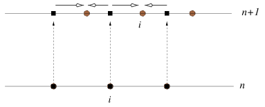
FIG. 1.: Illustration of the causal differencing strategy. First the integration proceeds along the dashed lines to obtain values in the $n+1$ level (at filled square points). Then, an interpolation is carried out to obtain values on the grid points (filled circles). In the graph, as an example, a second order interpolation (indicated with arrows) provides values on the i-th grid point.

A Numerical Implementation

In the numerical implementation of the CADM it is convenient to introduce an intermediate variable $F$ such that $\phi\equiv 1/4\ln(F)$ and evolve $F$ instead of $\phi$. This choice avoids unnecessary handling of exponential and logarithmic functions thus preventing loss of accuracy; hence, the equation for $F$ is

$$\partial_{o}F=-\frac{2}{3}\alpha FK+\frac{2}{3}F\beta^{i}_{,i}$$ (38)

A second order finite difference code has been written to implement both the ADM and CADM formulations. The same causal differencing algorithms have been applied to both formulations. These algorithms involve at their core, an interpolation for every grid point in the computational domain. Near an excision boundary the choice of interpolation order and stencil choice becomes important. We allow a choice of second, third and fourth order interpolations in order to study possible practical approaches .

IV Applications

To compare evolutions with the above formulations we pick as a particular example the Schwarzschild spacetime (and linear perturbations of it). In order to implement excision, a slicing must be chosen such that surfaces of constant time “penetrate” the horizon. The ingoing Eddington Finkelstein coordinates define hypersurfaces satisfying this condition; in terms of them, the line element reads

$$ds^{2}=-\left(1-\frac{2M}{r}\right)dt^{2}+\frac{4M}{r}dt\,dr+\left(1+\frac{2M}{r}\right)dr^{2}+r^{2}d\Omega^{2}\,,$$ (39)

where $d\Omega^{2}=d\theta^{2}+\sin^{2}\theta\,d\phi^{2}$. The lapse and shift vector are therefore:

$$\alpha=\sqrt{\frac{r}{r+2M}}\,,\,\beta^{i}=\frac{2M}{r+2M}\delta^{i}_{r}\,,$$ (40)

The basic ADM variables read

$$\gamma_{rr} = 1+2\frac{M}{r}\,;\,\gamma_{\theta\theta}=r^{2}=\frac{\gamma_{\phi\phi}}{\sin^{2}\theta}$$ (41)

$$K_{rr} = -\frac{2M}{r^{3}}(r+M)\alpha\,;\,K_{\theta\theta}=2M\alpha=\frac{K_{\phi\phi}}{\sin^{2}\theta}\,.$$ (42)

and the CADM variables

$$\tilde{\phi} = \frac{1}{4}\ln(\left[(r+2M)r^{3}\sin^{2}\theta\right]^{1/3})\,;\,K=\frac{2M\alpha}{r^{2}}\frac{(r+3M)}{(r+2M)}$$ (43)

$$\tilde{\gamma}_{rr} = \frac{r+2M}{r^{2}\left[(r+2M)\sin^{2}\theta\right]^{1/3}}\,;\,\tilde{\gamma}_{\theta\theta}=\frac{r}{\left[(r+2M)\sin^{2}\theta\right]^{1/3}}=\frac{\tilde{\gamma}_{\phi\phi}}{\sin^{2}\theta}$$ (44)

$$\tilde{A}_{rr} = -\frac{4M}{3}\frac{\alpha(2r+3M)}{r^{4}\left[(r+2M)\sin^{2}\theta\right]^{1/3}}$$ (45)

$$\tilde{A}_{\theta\theta} = \frac{2M}{3}\frac{\alpha(2r+3M)}{r(r+2M)\left[(r+2M)\sin^{2}\theta\right]^{1/3}}=\frac{\tilde{A}_{\phi\phi}}{\sin^{2}\theta}\,$$ (46)

$$\tilde{\Gamma}^{r} = -\frac{4}{3}\frac{r^{3}(r+3M)\sin^{2}\theta}{r^{2}(r+2M)^{5/3}}$$ (47)

$$\tilde{\Gamma}^{\theta} = -\frac{2}{3}\frac{r(r+2M)\cos\theta}{r^{2}(r+2M)^{2/3}\sin^{2/3}\theta}$$ (48)

$$\tilde{\Gamma}^{\phi} = 0\,.$$ (49)

Note that some of the quantities are functions of $\theta$. In our spherically symmetric implementation of these equations we have explicitly expressed each variable as a function of $r$ times the exact function of the angle $\theta$. For instance we write

$$\tilde{\gamma}_{\theta\theta}=h_{\theta\theta}(r)/\sin^{2}\theta\,.$$ (50)

Proceeding this way allows for the explicit appearance of $\theta$ to drop out of the equations, providing at the end of the day, a truly $1D$ system of equations corresponding to spherical symmetry.

A Comparison

Extended tests were performed with both codes (under the same conditions) to understand the robustness of each formulation with excision. As has been observed in previous work[7, 11], CADM gives long term evolutions when the evolution of $K$ is “frozen”; ie the equation for $K$ is not evolved or the value of $K$ is fixed by the choice of a slicing that leaves $K$ fixed (for instance, maximal slicing that fixes $K=0$.). On the other hand, longer term evolutions have also been achieved with an area locking gauge in the ADM formulation[22]. We then perform three basic tests:

• Fully free evolution: All equations corresponding to each system are integrated without imposing any further condition

• “Locked” evolution: Conditions on some of the field variables are enforced (see below).

• “Perturbed” evolution: Same as the “locked” case but considering linear perturbations of Schwarzschild spacetime as initial data

In all these tests, we study the dependence of the obtained solution under discretization size and location of the outer boundary. The inner boundary is placed at $r=M$ and the outer boundary is varied (placed at $r=nM$) while keeping $\Delta r=const$. Outer boundary data are provided by ‘blending’[23] the numerical solution to the analytical one. This choice reduces gradients and second derivatives at the boundary allowing for a clean evolution without much reflections from the outer boundary.

1 Fully free evolution

In this case, all equations corresponding to systems (III,III) are evolved and the obtained solutions are compared. We use the Hamiltonian and momentum constraint as monitors of the quality of the evolution. Our results can be summarized as follows. For the ADM formulation we observed that stable evolutions are obtained if $n<6$ while for larger $n>6$ the solution exhibits exponentially growing modes. It is worth emphasizing that the evolution is not unstable under the strict sense (i.e. the solution can be bounded from above by an exponential[24].). However, the presence of this exponential mode will likely spoil any long term simulation. For the CADM system, irrespective of the value of $n$ exponential modes are clearly present in the solutions.

These results are illustrated in Fig.2, which shows the $L_{2}$ norm of the Hamiltonian and momentum constraints of the solutions obtained with both formulations when $n=4$. Clearly, the solution obtained with the ADM is better than that obtained with the CADM. Figure 2, also displays the $L_{2}$ norm of the Hamiltonian constraint for the case $n=9$, although the solution obtained with the ADM formulation can be considered better than that from the CADM, both grow exponentially.

FIG. 2.: The $L_{2}$ norm of the Hamiltonian and momentum constraints for both formulations (discretization size $\Delta r=M/10$) for the case where the domain of integration is $[M,4M]$ (A) and $[M,9M]$ (B). In A, the evolution obtained with the ADM formulation does not show the presence of an exponentially growing mode like the one obtained with the CADM approach. However, for the larger domain, (B), solutions obtained with both formulations are exponentially growing.

2 Locked evolution

It has been observed in the literature[11] that in the case where $K$ is fixed in time very long term evolutions can be obtained with the CADM system. It is interesting to see what this condition implies, note that if $K$ does not vary, then, $\phi$ will remain unchanged and therefore the determinant of the three metric $\gamma_{ij}$ will remain independent of time. This, could be regarded as an evolution that “locks” the volume and bears some similarity with the so-called “area-locking” gauge[16, 22]. It is also worth pointing out that a similar strategy can be implemented in the ADM case as it has been shown in[22]. In this work, by choosing a gauge that “locks” the evolution of $g_{\theta\theta}$ the exponentially growing modes displayed by solutions in domains with $6<n<11$ are removed. Figure 3 shows the $L_{2}$ norm of the Hamiltonian and momentum constraints corresponding to solutions obtained with both formulations for the choice $n=4$ and $n=9$. In both cases the simulations can be performed for unlimited time without observing exponential modes. Again, the solution obtained with the ADM formulation is slightly more accurate than that provided by the CADM formulation.

It is important to observe that for the CADM case with $K$ frozen, evolutions without exponentially growing modes are obtained with $n$ as large as $16$. For $n>16$ long term evolutions ($>100M$) display at late times a clear exponentially growing mode.

FIG. 3.: The $L_{2}$ norm of the Hamiltonian and momentum constraints for both formulations (with $\Delta r=M/10$) for the case where the domain of integration is $[M,4M]$ (A). Neither formulation displays exponential modes in this domain and the ADM one yields more accurate results. In B, the $L_{2}$ norm of the Hamiltonian and momentum constraints of the solution obtained with the CADM and an “area-locked” ADM evolution (in the $[M,9M]$ domain) is shown, a transient oscillatory behavior is present at earlier stages and the solutions then settle to a constant value.

3 Perturbed evolution

In this case, we test the evolutions under perturbations (using a locked evolution in the CADM case but not in the ADM one). The initial data corresponds to the analytic value of $\gamma_{rr}$ (or $\tilde{\gamma}_{rr}$) plus some arbitrary pulse of compact support. Of course, this data is unphysical but we use it to probe for stability of the implementations in a non-trivial scenario. The amplitude of the pulse is chosen such that it can be considered a linear perturbation of a Schwarzschild spacetime. The results obtained with both codes agree with those of the previous section. Figure 4 corresponds to the evolution of a pulse with compact support in $[3M,5M]$ being evolved in a computational domain of $[M,6M]$. The $L_{2}$ norm of the Hamiltonian constraint, after some initial transient behavior, settles into a stationary regime.

FIG. 4.: The $L_{2}$ norm of the Hamiltonian constraint for the perturbed evolutions (where $K$ has been frozen in the CADM evolution while all fields are evolved in the ADM one). After some initial transient behavior both settle into an stationary solution.

B Locking evolutions

As mentioned, in previous work[11], by not evolving the equation for $K$ very long term evolutions have been achieved with the CADM formulation. However, choosing to do so is unphysical in generic situations. One would like to have a prescription where a similar condition can be enforced without having to not evolve one or more equations. Here, one can use the gauge freedom of the theory to demand that $\partial_{t}K=0$. This in turns implies a condition of the shift vector from equation (32),

$$\beta^{i}\partial_{i}K=\gamma^{ij}D_{i}D_{j}\alpha-\alpha\left[\tilde{A}_{ij}\tilde{A}^{ij}+\frac{1}{3}K^{2}\right]\,.$$ (51)

This condition is straightforward to implement in 1D but is certainly more complicated in 3D. Additionally, there is a great deal of ambiguity as it is only one equation for three variables $\beta^{i}$. Therefore two supplementary conditions must be chosen so that (51) can be used to ‘freeze’ the evolution of $K$. In our present implementaion we have simply chosen $\beta^{A}=0$ (with $A=(\theta,\phi)$) and obtain $\beta^{r}$ with (51) as

$$\beta^{r}=\frac{1}{\partial_{r}K}\left(\gamma^{ij}D_{i}D_{j}\alpha-\alpha\left[\tilde{A}_{ij}\tilde{A}^{ij}+\frac{1}{3}K^{2}\right]\right)\,.$$ (52)

A simple way to obtain $\beta^{r}$ is by a first order approximation of the rhs of Eq. 52 (ie. evaluating each term at the old level). By using this condition, instead of choosing not to evolve $K$, we were able to obtain evolutions not displaying exponential modes for times larger than $250M$ (with resolutions of $\Delta r=M/10$ and finer). Figure 5 illustrates what is obtained in a simulation with computational domain defined by $[M,11M]$ (with $\Delta r=M/10$). The values of the $L_{2}$ norms of the Hamiltonian, the function $F-F_{t=0}$ and value of $K-K_{t=0}$ are shown as a function of time. Since $\beta^{r}$ is obtained only as a first order approximation, $K$ and $F$ are expected to vary during the evolution. As can be seen in Fig. 5, both grow linearly but stay fairly close to zero and the evolution proceeds without displaying an exponential growth.

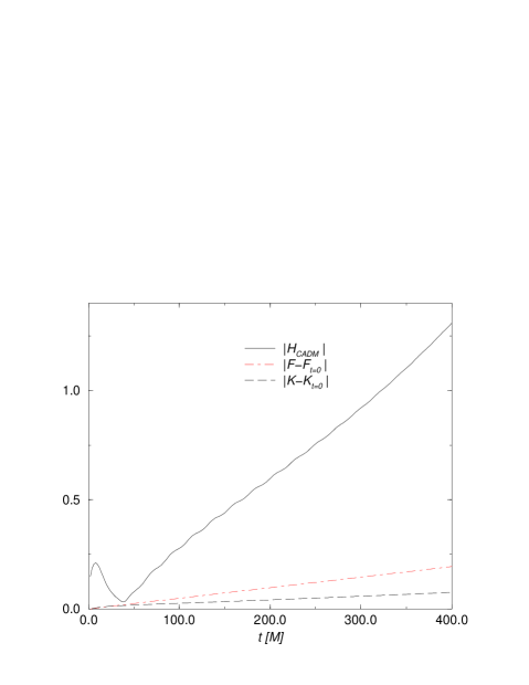
FIG. 5.: The $L_{2}$ norms of the Hamiltonian constraint and the differences $F-F_{t}=0$ and $K-K_{t=0}$ vs. time. The evolution proceeds without displaying exponential modes and the value of $|K-K_{t=0}|$ stays close to zero.

C Causal differencing and domain of dependencies

As a last point, it is interesting to see how causal differencing is indeed providing a correct way to discretize the equations taking advantage of the causal properties of the spacetime. The fact that the null cones (or the causal domain of dependence) are tilted inside the horizon, allows for a stable numerical implementation where inner boundary data need not be provided if the inner boundary is inside the black hole (see Fig. 6). This is possible because the numerical domain of dependence naturally contains the domain of dependence of the inner boundary point. This is of course, not true if the innermost point is outside the event horizon. In order to illustrate this fact we compare $2$ cases (with both formulations) where the innermost point is placed inside or just outside the event horizon. As illustrated in Fig. 7, while the solution obtained with the inner boundary inside the black hole is stable, the other, as expected is unstable.

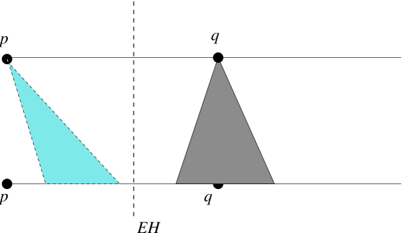
FIG. 6.: Domains of dependence of points inside and outside the event horizon (EH). Inside the EH, the past null cone of $p$ is tilted, therefore the evolution algorithm does not need the value of the fields at $p$ on the old level.

FIG. 7.: The $L_{2}$ norm of the Hamiltonian constraint for the cases where the inner boundary is inside (at $r=1.5M$ denoted with a solid line) and outside (at $r=2.2M$ denoted with a dashed line) the event horizon (using the ADM formulation). Since the latter does not respect the CFL condition, the obtained solution is unstable. (The values shown correspond to a discretization of size $\Delta r=M/10$ and no qualitative difference is observed with finer resolutions.)

V Conclusions

The results presented in this work show that excision techniques can be straightforwardly used in the CADM formulation directly from the structures developed for the ADM formulation.

The ADM formulation is superior to the CADM both in accuracy and total time evolution when the evolution of $K$ is not locked in CADM. When locking is implemented, then CADM is better than ADM as the solution obtained with the CADM formulation does not display exponential modes with the outer boundary placed as far as $16M$. On the other hand, evolutions with the ADM formulation display exponential modes with the outer boundary placed at $11M$ and beyond. Additionally, for the case where outer boundaries are placed ‘very’ far, although exponentially growing solutions are present in solutions obtained with both formulations, ADM simulations crash at earlier times than CADM.

It is worth remarking again that in both formulations, implementing a gauge that minimizes the changes in some of the fields (like $g_{\theta\theta}$ in the ADM formulation or $K$ in the CADM one) dramatically improves the evolutions in 1D. In the 3D case, the use of ‘area or circunference locking’ is indeed more complicated than locking $K$, simply by the fact that in the former case one is trying to control a tensor component while in the latter a scalar. Thus, locking $K$ is likely to have an easier and probably more general implementation than area locking (although in cases where the final black hole is close to a non spinning one, this implementation is rather straightforward). Controling the evolution of $K$ demans a condition like that given by Eq (51), and two extra conditions on $\beta^{i}$ will be required. An option that could mimic the 1D implementation would be to foliate the 3D hypersurfaces with a sequence of 2-surfaces defined by $\Theta=const$ (with $\Theta$ the expansion of outgoing null rays). Once this foliation is obtained, the shift vector $\beta^{i}$ could be decomposed as

$$\beta^{i}=\beta^{i}_{|\ }+\beta^{i}_{\bot}$$ (53)

with $\beta^{i}_{|\ }$ ($\beta^{i}_{\bot}$) parallel (perpendicular) to the normal of the 2-surfaces. Thus, the two further conditions can be chosen such that $\beta^{i}_{\bot}=const$. This will thus minimize changes in transversal directions and will resemble that we have used in the 1D case. Of course, this is just one possible approach and further studies will be required to obtain a $K$ fixing condition that leads to a practical implementation.

In conclusion, implementing singularity excision techniques in the CADM formulation is straightforward. The usefulness of this implementation depends on implementing a gauge controlling the behavior of $K$. Assuming this can be achieved, CADM appears to be capable of providing more robust simulations than ADM when the outer boundary is placed farther than $11M$ from the final black hole of mass $M$, if the outer boundary is closer, then the ADM formulation provides evolutions as stable as the CADM one but with better accuracy.

As a last remark, it is important to stress that we have only implemented the causal differencing algorithm described in[20, 19] since at present is the only one fully implemented in $3D$. Other alternatives have been proposed[17, 18, 25]; due to the restriction to spherical symmetry it is likely that the application of these will yield similar results to those presented in this work.

- [1] M. Huq. Proceedings of the BBH Grand Challenge Meeting. Pittsburgh, PA 1997.
- [2] G. Gook and M. Shceel. Proceedings of the BBH Grand Challenge Meeting. Austin, TX 1998.
- [3] J. Thornburg, Class. and Quantum Grav., 14, 1119 (1987).
- [4] For instance, H. Friedrich, Proc. Roy. Soc. Lond. A375, 169 (1981). S. Frittelli, O. Reula, Phys. Rev. Lett, 76, 4667, (1996). A. Anderson and J. York, Phys. Rev. Lett, 82, 4384, (1999). (For a detailed list of hyperbolic formulations see O. Reula, Living Reviews in Relativity (1998)).
- [5] C. Bona, J. Masso, E. Seidel and J. Stela, Phys. Rev. D., 56, 3405 (1997).
- [6] M. Shibata and T. Nakamura Phys. Rev. D., 52, 5428 (1995).
- [7] T. Baumgarte and S. Shapiro. Phys. Rev. D., 59, 024007 (1999).
- [8] S. Frittelli and O. Reula, gr-qc/9904048 (1999).
- [9] L.L.Smarr and J.W.York, Phys. Rev. D., 17(10), 2529-2551 (1978). P.R. Brady, J.D. Creighton and K.S. Thorne, Phys. Rev. D., 58, 061501 (1998). C. Gundlach and D. Garfinkle., Class. Quant. Grav., 16 (1999).
- [10] K. Oohara and T. Nakamura ‘3D General Relativistic Simulations of Coalescing Binary Neutron Stars’, astro-ph/9912085 (1999).
- [11] M. Alcubierre, G. Allen, B. Brügmann, T. Dramlitsch, J. Font, P. Papadopoulos, E. Seidel, N. Stergioulas, W. M. Suen and R. Takahashi. ‘Towards a stable numerical evolution of strongly gravitating systems in General Relativity’. gr-qc/0003071, (2000).
- [12] B. Brügmann, Int. J. Mod. Phys. D8, 85 (1999).
- [13] The Binary Black Hole Grand Challenge Alliance, Phys. Rev. Letters, 80, 2512 (1998).
- [14] R. Marsa and M. Choptuik, Phys. Rev. D., 54, 4929 (1996).
- [15] C. Misner, K. S. Thorne, and J. Wheeler, Gravitation (W. H. Freeman and Co., San Francisco, 1973).
- [16] E. Seidel, W.M. Suen, Phys. Rev. Letters 69 (1992).
- [17] M. Alcubierre and B. Schutz, J. Comp. Phys. 112 (1994).
- [18] C. Gundlach and P. Walker, Class Quant Grav 16 991-1010 (1999)
- [19] M. Scheel, T. Baumgarte, G. Cook, S. Shapiro and S. Teukolsky, Phys. Rev. D., 56, 6320 (1997).
- [20] M. Huq and R. Matzner, “BBHGC Alliance Cauchy Code Documentation”, unpublished.
- [21] http://www.astro.psu.edu/users/nr/Agave/.
- [22] L. Lehner, M. Huq, M. Anderson, E. Bonning, D. Schaefer and R. Matzner, to appear in Phys. Rev. D., (2000).
- [23] R. Gomez. Proceedings of the BBH Grand Challenge Meeting. Los Alamos, NM 1997.
- [24] B. Gustaffson, H. Kreiss and J. Oliger. Time Dependent Problems and Difference Methods (John Wiley & Sons, New York, 1995).
- [25] R. Gomez, L. Lehner, R. Marsa and J. Winicour, Phys. Rev. D., 57, 4778 (1998).