Generic Tracking of Multiple Apparent Horizons with Level Flow

Abstract

We report the development of the first apparent horizon locator capable of finding multiple apparent horizons in a “generic” numerical black hole spacetime. We use a level-flow method which, starting from a single arbitrary initial trial surface, can undergo topology changes as it flows towards disjoint apparent horizons if they are present. The level flow method has two advantages: 1) The solution is independent of changes in the initial guess and 2) The solution can have multiple components. We illustrate our method of locating apparent horizons by tracking horizon components in a short Kerr-Schild binary black hole grazing collision.

]

I Introduction

Our goal is to investigate the strong field regime of general relativity. In particular we wish to focus on the study of coalescing black hole binaries. Over the last three decades since the pioneering work of Cadez, Smarr, Eppley and others, advances in computing technology, numerical algorithms and techniques and our understanding of the underlying physics have advanced to a point where we are able to carry out simulations of binary black hole collisions in 3+1 dimensions. One of the outcomes of such simulations will be an understanding of the underlying physics of the problem; and, therefore, a prediction and understanding of the gravitational radiation content. A detailed knowledge of how the resultant gravitational waveforms relate to the physical parameters of the binaries that produce them will be of importance to gravitational wave observatories (such as LIGO, VIRGO, TAMA, GEO600) now under construction around the world. With the building of these observatories, we stand at the epoch of the first direct observations of astrophysical sources that involve strong field general relativity.

The orbit and merger of two black holes is one candidate source for ground based detection of gravitational waveforms. This is of great interest to the relativity community. The binary black hole problem is a two-body problem in general relativity. It is a stringent dynamical test of the theory. However, studying spacetimes containing multiple black holes involves solving the Einstein equations, a complex system of non-linear, dynamic, elliptic-hyperbolic equations intractable in closed form. The intractability of the problem has led to the development of numerical codes capable of solving the Einstein equations.

Our approach to numerically solving the Einstein equations involves reformulating them as an initial value problem. In this 3+1 formulation [1], spacelike hypersurfaces parameterized in time foliate the spacetime. The resulting equations are coupled elliptic and hyperbolic differential equations of the 3-metric, $g_{ij}$, and the extrinsic curvature, $K_{ij}$. The initial value problem is solved by specifying a hypersurface at an instant of time, say $t=0$, and evolving to the next hypersurface at time $t=\delta t$ with the evolution equations to obtain $g_{ij}$ and $K_{ij}$ at the next time $t=\delta t$.

One vital issue in numerically solving the Einstein equation describing spacetimes containing black holes is handling the physical singularities. As one approaches the singularity, the values of the fields being computed approach infinity; therefore, a region containing the singularity must be avoided to keep the computation from halting. Excision techniques are promising in avoiding the singularity. Excising the singularity involves locating a region interior to the event horizon containing the singularity on each evolving hypersurface. This region is then “masked” from the computation. The derivatives at the boundary between the masked region and the computational domain are handled using causal differencing, a differencing scheme[2] that respects the causal structure of the spacetime.

In deciding where in space to excise we use the apparent horizon as opposed to the event horizon. By its very nature, the event horizon is a global construct depending on the entire spacetime. The apparent horizon, a local, i.e. spacelike 2-surface is more suitable. Following a suggestion by Unruh [3], the apparent horizon is used to define the excised region to be masked at each time during the evolution. Apparent horizons are defined locally for each time, and exist at, or inside of, the event horizon. In some spacetimes, choices of foliation may lead to the absence of an apparent horizon. When the discussions in this refer to a hypersurface, it is assumed an apparent horizon exists on that hypersurface.

Recent three-dimensional horizon locator codes are capable of finding the location of an apparent horizon in generic single black hole spacetimes [4, 5, 6, 7, 8, 9] and two [10, 11] are capable of finding disjoint multiple apparent horizons in the special case of conformally flat binary, time-symmetric black hole spacetimes. Multiple apparent horizon finding algorithms will be necessary in simulations of generic binary black hole spacetimes. The method presented in this paper, called the level flow method, is capable of detecting multiple apparent horizons in generic spacetimes. The level flow algorithm has two advantages: 1) It is independent of a good initial guess and 2) It is capable of following the surface through a change in topology. In level flow, the apparent horizon equation is reformulated as a parabolic equation and a set of surfaces are flowed with speeds dependent on the expansion of the outgoing null vectors normal to each surface.

The purpose behind developing the level flow method of tracking apparent horizons is to have a method capable of detecting multiple apparent horizons on any given hypersurface without a good guess. Specifically, we want a tracker that can detect the transition from a double to a single apparent horizon in single time step without a prior knowledge of the transition.

In the rest of this paper we discuss apparent horizons in general and current 3D work in $\S~{}\ref{sec:ah}$ and $\S~{}\ref{sec:method}$. In $\S~{}\ref{sec:LFM}$ we describe the level flow method in detail and give a brief description of the numerical method involved in solving the apparent horizon is in $\S~{}\ref{sec:NM}$. We demonstrate the use of the level flow tracker on model data and a binary black hole grazing collision in $\S~{}\ref{sec:testing}$ and $\S~{}\ref{sec:graze}$.

II Apparent Horizons

FIG. 1.: Representation of a 2-sphere embedded in a hypersurface, $\Sigma$.

$M$ is the spacetime with metric ${}^{4}g_{ab}$ foliated by hypersurfaces $\Sigma$ parameterized by $t$ with 3-metric $g_{ab}$. Let $S$ be a surface with $S^{2}$ topology on $\Sigma$. The apparent horizon is the outermost marginally trapped surface in $\Sigma$, a surface with zero expansion. The zero expansion of the surface is defined in terms of outgoing null vectors to $S$, $k^{a}$, such that $k^{a}$ have zero divergence

$$\nabla_{a}k^{a}=0,$$ (1)

where $\nabla_{a}$ is the covariant derivative associated with ${}^{4}g_{ab}$. Referring to fig. (1), $k^{a}$ is defined in terms of the spacelike normals to $S$, $s^{a}$, and the future directed timelike normals, $n^{a}$, such that:

$$k^{a}=s^{a}+n^{a}.$$ (2)

The expansion of the outgoing normals, $\nabla_{a}k^{a}$, can be rewritten in terms of quantities defined on the hypersurface:

$$\kappa\equiv D^{a}s_{a}-K+s^{a}s^{b}K_{ab}.$$ (3)

$D_{a}$ denotes covariant differentiation with respect to $g_{ab}$, $K_{ab}$ is the extrinsic curvature, and $K$ is $g^{ab}K_{ab}$. In fact, there is a level set of surfaces in $\Sigma$ parameterized by $\kappa$. Each surface in the level set is defined by the constant expansion of its null vectors such that

$$\kappa=c_{n},$$ (4)

where $c_{n}$ are constants labeled by the positive integer $n$. Marginally trapped surfaces are members of this set for

$$\kappa=0.$$ (5)

Eqn.(5) is called the apparent horizon equation since the apparent horizon is the outermost surface with $\kappa=0$ in $\Sigma$.

The $S^{2}$ topology of the apparent horizon naturally lends itself to characterization via spherical coordinates. The function,

$$\psi=r-h(\theta,\phi)$$ (6)

is a level set of 2-spheres in $\Sigma$, where $h(\theta,\phi)$ is called the apparent horizon shape function. A marginally trapped surface has $\psi=0$. The spacelike normals to $S$ are defined from eqn. (6) such that

$$s^{i}=g^{ij}\partial_{j}\psi/\sqrt{g^{kl}\partial_{k}\psi\partial_{l}\psi}$$ (7)

is the spacelike vector field at every point of $S$. The apparent horizon equation in spherical coordinates ($h(\theta,\phi),\theta,\phi$) is a 2-dimensional problem in $\theta$ and $\phi$.

III Current 3-D Methods

The approaches to solving the apparent horizon equation on a three-dimensional hypersurface can be addressed roughly in two categories: methods that solve the apparent horizon equation directly and methods that solve it by first recasting it as a parabolic equation. This paper does not address spherical and axi-symmetric approaches. One of the first three-dimensional apparent horizon solvers was published by Nakamura, Kojima, and Oohara [9]. They directly solve the apparent horizon equation by using spherical harmonic basis functions to expand the apparent horizon shape function, $h(\theta,\phi)$ into

$$h(\theta,\phi)=\sum^{l_{max}}_{l=0}\sum^{l}_{m=-l}a_{lm}Y_{lm}(\theta,\phi).$$ (8)

This method is called the pseudospectral method. A finite number of the coefficients, $\{a_{lm}\}$ parameterize the horizon shape function, and the maximum $l_{max}$ depends on the computation and deviations from a sphere. The apparent horizon equation can then be solved by writing it as

$$\|\kappa(a_{lm})\|=0,$$ (9)

and using functional integration routines to find the coefficients $a_{lm}$. Others have used similar methods [5, 8, 4].

In another approach to direct solutions of the apparent horizon equation is to treat it as a boundary value problem. One notes that a discretization of this equation leads to a system of algebraic equations which can then be solved via Newton’s method. Thornburg [12] discusses applications of Newton’s method to this problem in general and shows results in axisymmetry. Huq [13] has implemented a similar algorithm based on Newton’s method that utilizes Cartesian coordinates to difference the equations.

Tod [14] first suggested the use of curvature flow in solving the apparent horizon equation by recasting it as a parabolic equation. Bernstein [15] implemented Tod’s suggestion in axisymmetry. Gundlach [6] introduced a fast flow method which combines the ideas of the flow method with the pseudospectral method. Pasch [11] and Diener [10] implemented a similar method, a level-set method, in three-dimensions and found discrete apparent horizons in multi-black-hole spacetimes; however these spacetimes were confined to be conformally flat and time-symmetric.

Each of the approaches briefly described above, solving the apparent horizon equation directly or solving it via a parabolic equation, has its advantages. Direct methods tend to be faster while flow methods do not rely on “good” initial guesses. However, none of these methods are applicable to the generic, multi-black-hole problem. Herein lies the motivation behind the level flow method. The level flow method is the only method designed to locate discrete apparent horizons in generic spacetimes containing one or two discrete horizons.

IV Level Flow Method

A Curvature Flow

The level flow method is a hybrid flow$/$level$-$set method. The previous section mentioned the flow method, this section gives more detail on the flow method which is the foundation of the level flow method. The flow approach, as suggested by Tod, is to rewrite the apparent horizon equation as the speed function in a parabolic equation. In the case of a time symmetric hypersurface, in which $K_{ab}=0$, the apparent horizon equation reduces to the condition for a minimal surface, $D_{a}s^{a}=0$. In this case, the surface $S$ is at a local extremum of the area. The starting surface, $S(\lambda=0)$, is parameterized by coordinates $x^{a}$ and evolved in terms of a parameter $\lambda$. The equation of motion is

$$\frac{\partial x^{a}}{\partial\lambda}=-Hs^{a}$$ (10)

where $\partial x^{a}/\partial\lambda$ is a vector field, and $H$ is the mean curvature, which is the trace of extrinsic curvature associated with embedding $S$ in $\Sigma$ given by

$$H=D_{a}s^{a}.$$ (11)

Eqn.(10) is the gradient flow for the area functional. The area decreases monotonically with increasing $\lambda$. Grayson [16] has shown that a surface deforming under its gradient field (Eqn.(10)) will evolve to a stable minimum surface (surface is local minimum of area) if there is one, otherwise to a point.

In numerical relativity, we are interested in the generic case, with $K_{ab}\neq 0$, for which the marginally trapped surfaces differ from minimal surfaces, the surfaces are not extrema of the area. However, Tod suggests an equation similar to Eqn.(10) as a curvature flow:

$$\frac{\partial x^{a}}{\partial\lambda}=F(\kappa)s^{a}$$ (12)

using $F(\kappa)=-\kappa$ where $\kappa=D_{a}s^{a}+s^{a}s^{b}K_{ab}-K$ as in eqn.(3). We have found eqn. (12) to be a successful practical implementation of the flow method.

B Level Flow

Eqn. (12) gives us an initial value problem. Given information about the system at some initial $\lambda$, eqn. (12) will describe the system for all its future propagation in $\lambda$. Directly solving eqn. (12) will lead to a successful detection of single apparent horizons; however, solving it directly does not ensure correct handling of a topology change which is necessary for detection of multiple apparent horizons. By combining the flow method with a level-set idea however, this topology change can be effected and multiple apparent horizons can be tracked starting from a single guess surface.

First eqn. (12) is recast from an equation governing the motion of the coordinates parameterizing $S$, namely $x^{a}$, to an equation governing the motion of the surface $\psi$. Noting that $\psi$ is parameterized by $\lambda$,

$$\frac{\partial\psi}{\partial\lambda}=\frac{\partial x^{a}}{\partial\lambda}\frac{\partial\psi}{\partial x^{a}}$$ (13)

by the chain rule, and multiplying eqn.(12) by $\frac{\partial\psi}{\partial x^{a}}$ gives

$$\frac{\partial\psi}{\partial\lambda}=F(\kappa)s^{a}\partial\psi/\partial x^{a}.$$ (14)

Using

$$s^{a}=g^{ab}\frac{\partial\psi}{\partial x^{b}}/\|\nabla\psi\|$$ (15)

and

$$\|\nabla\psi\|=\sqrt{\frac{\partial\psi}{\partial x^{a}}\frac{\partial\psi}{\partial x^{b}}g^{ab}},$$ (16)

the test surface’s flow is given by:

$$\frac{\partial\psi}{\partial\lambda}=F(\kappa)\|\nabla\psi\|.$$ (17)

Eqn.(17) is a reformulation of eqn. (12) and will flow the surface, $\psi$, to a marginally trapped surface at $\psi=0$ when $\kappa=0$.

The strength of the flow methods is their ability to locate a surface with $\kappa=0$ given any non-pathological initial surface. For example, the apparent horizon in a spherically symmetric spacetime (Schwarzschild) was found by flowing an initial surface shaped as a leaf, see Fig. (2). This ability is especially important when tracking horizons during evolutions of binary black hole spacetimes. In this case, finding apparent horizons for two discrete apparent horizons in each $\Sigma(t)$ involves flowing two initial guesses, one for each horizon [17]. On $\Sigma(t=0)$, the location of the apparent horizons may be known; however, as the black holes accelerate the task of guessing the locations of the two horizons becomes more difficult. Further, the two horizons merge into a single horizon at a single instant of time, rendering a good initial guess difficult. Some way of determining when two horizons merge into a single horizon is necessary. The level flow method takes care of these issues by not requiring a good initial guess $(\psi(\lambda=0))$ and by detecting multiple apparent horizons from a single guess $(\psi(\lambda=0))$.

FIG. 2.: Example of a surface undergoing flow on a spherically symmetric hypersurface. The figure labeled (a) is $\psi(\lambda=0)$, the initial guess. Figure (b) is $\psi(\lambda)$ representing the final solution, the apparent horizon.

The level flow method differs from the flow method in the specification of the speed function, $F(\kappa)$. $F(\kappa)=0$ determines when the propagation of the surface stops. The flow method is in the form of eqn. (12), in which $F(\kappa)=-\kappa$. A good choice since $F(\kappa)=-\kappa=0$ indicates a marginally trapped surface; but this choice will not flow $\psi$ though a fission. In general the scheme fails as the surface pinches due to ill-defined normals at the surface. The level flow method alleviates this problem by looking for indications that the surface topology is about to change before the pinching occurs. (Another method which was introduced by Sethian and Osher [18] for non-relativistic problems is to flow a higher dimensional surface in which $\psi$ is embedded. This higher dimensional surface does not fission. This has only been implemented in a time-symmetric spacetime [11] and requires more computational power due to the extra dimension in the problem.)

The level flow method flows a set of two-dimensional surfaces in $\Sigma$ parameterized by $\kappa$. We call the set of surfaces a level set and label the set $S(c_{n})$. Each surface has a constant value of $\kappa=c_{n}$ everywhere on it. The set of surfaces is defined by varying $c_{n}$ as the flow progresses

$$c_{n+1}=c_{n}\pm\Delta c,$$ (18)

where $(+)$ indicates outward flow, $(-)$ inward flow, and $\Delta c\propto\parallel\kappa\parallel_{2}$. Each surface obeys the equation of motion given in eqn. (17) with $F(\kappa)$ defined to flow to multiple surfaces. We choose two options for the speed function:

$$F(\kappa) = \kappa-c_{n}$$ (19)

$$F(\kappa) = (\kappa-c_{n})\arctan^{2}(\frac{\kappa-c_{n}}{\kappa_{o}}).$$ (20)

As $\kappa-c_{n}\rightarrow 0$, both functions are solving for a particular surface in the level set, $S(c_{n})$. The second function, eqn.(20), behaves similarly to the first but allows for larger time steps near a fissioning surface because it moves points further from the $\kappa-c_{n}=0$ surface faster than the points closer to this surface.

Eqn. (17) is an initial value problem requiring $\psi$ to be specified at $\lambda=0$. To initialize the starting surface, we need only supply an origin and radius. Taking into account that there may be more than one marginally trapped surface, it is best to start with an initial surface larger than the expected horizon. The values of $g_{ij}$ and $K_{ij}$ are required everywhere on the surface to evaluate $\kappa$. These functions can be known analytically or generated by evolution codes. As the flow velocity approaches zero, $F(\kappa-c)\rightarrow 0$, $\kappa\sim c_{n}$ and a surface $S(c_{n})$ is found within a tolerance ($\epsilon_{\kappa}$). When $\kappa=0$, the located surface describes a marginally trapped surface.

FIG. 3.: Schematic of $\psi(c_{n})$, the level set of surfaces in $\Sigma(t)$. We solve for a single surface, $S(c_{n})$, in $\psi(c_{n})$. Multiple levels are used in detecting the existence of multiple horizons.

FIG. 4.: Plot of five levels ($\kappa$ = 0.14,0.12,0.10,0.08,0.06) of constant divergence of outgoing null geodesics.

Fig.(4) shows the level set found in a spacetime containing two black holes with coordinate locations $(-0.954,0,-0.3)M$ and $(0.954,0,0.3)M$. Each 2-surface has a constant value of $\kappa$. We monitor the topology of the deforming surface by computing the radial component of the gradient of $\kappa$ with respect to the normals of each surface in the level set. The gradient is defined as:

$$\frac{\|\kappa_{n-1}-\kappa_{n}\|}{\|\psi_{n-1}-\psi_{n}\|},$$ (21)

where $\psi$ is the function given in eqn.(6). A sharp increase in the gradient indicates the existence of multiple surfaces. To ensure that we do not erroneously abandon a single surface, we also monitor the maximum of the $l_{2}$-norm of $\kappa$. If $\kappa$ is no longer decreasing, we are no longer finding a solution to eqn.(4); otherwise the single surface is retained. The level flow method is essentially a special set of surfaces with properties that let us determine when to break. If we only flowed to $\kappa=0$, we would not form the collection of $\kappa=$constant surfaces.

Once a topology change is indicated, the radii and origins for each of the new surfaces are found (note that these four parameters for each surface are all that is needed to initiate two new trial surfaces). These origins and radii are determined using the location of the last of the single surfaces. Using this last single surface, we can find the origin of the last surface and the location on the surface with minimum gradient of the value of $\kappa$. This occurs at the farthest points from the pinching in the surface. Picture (a) in fig. (5) shows the last single surface with an arrow drawn from the origin to the point on the surface with a minimal change in $\kappa$. The arrow indicates a chosen direction. All points lying in this direction are collected and averaged to find a radius and center of mass. All points lying in the opposite direction are also collected and used to calculate the radius and center of mass for the second surface using the dotted arrows in picture (b) of fig.(5). These two sets of radii and centers are the initial starting parameters for each new trial surfaces. The tracker then flows the two new surfaces depicted in (c) of fig.(5) until $\kappa=0$ within $\epsilon_{\kappa}$.

FIG. 5.: Two-dimensional schematic representation of the three-dimensional decision process to identify the two surfaces that will evolve to the two apparent horizons. Fig. (c) depicts the two surfaces that will act as new test surfaces.

The level flow code is only started by the user once, the subsequent flowing to multiple apparent horizons is done automatically.

The advantage to the level flow method is its capability to detect apparent horizons in generic, multiple black hole spacetimes from a single reasonable initial guess. The drawbacks are the dependence of $\Delta\lambda$ on the spatial grid size, $\Delta\lambda\sim N^{-2}$ where $N^{2}=N_{\theta}N_{\phi}$ is the number of grid points, and the fact that we flow to a speed of zero (the flow speed approaches zero as $\kappa$ approaches zero). When using apparent horizon tracking in our evolution code, we will not require knowledge of the apparent horizon location to high precision; in fact we can find a surface with $\kappa\leq 0$ to remove the singularity thus alleviating some of the speed issues. Nonetheless, we plan to improve the speed of this algorithm. Some improvements have already been made to increase the efficiency of the current algorithm. The addition of the $\arctan^{2}$ function, eqn.(20), speeds up the algorithm during the fissioning process. Monitoring the number of steps needed to complete a Crank-Nicholson iteration (see $\S$V)) has also proven useful in increasing efficiency.

V Numerical Method

The previous section described how the level flow method is used to solve the apparent horizon equation. The resulting parabolic equation is updated using an iterative Crank-Nicholson method updating the variables at every $\lambda$-step. Iterative Crank-Nicholson converges to an exact solution of the implicit problem. However, the detailed behavior of this convergence [19] shows that the Crank-Nicholson solution at a particular iteration has an amplification factor $|{\cal{A}}^{(n)}|$ that oscillates around unity. The behavior varies in pairs: $|{\cal{A}}^{(n)}|<1$ for $n=2,3$; $|{\cal{A}}^{(n)}|>1$ for $n=4,5$, etc. while $|\hskip 2.84544pt|{\cal{A}}^{(n)}|-1|\rightarrow 0$ monotonically as $n\rightarrow\infty$. $n$ is counting the number of iterations it takes to get $\hat{\kappa}=\kappa$ within the specified tolerance. For the data presented here, a Crank-Nicholson iteration of $n=2$ or $n=3$ was maintained for errors less than the spatial grid spacing squared, $h^{2}$.

The spatial derivatives are approximated to second order in truncation error using centered finite differencing molecules. To verify the convergence of the level flow code, we include a plot of the convergence factor versus the number of iterations taken in fig. (6).

FIG. 6.: Convergence factor for radial variable $\kappa$ with $h=0.05$, $2h=0.10$, $4h=0.20$, and $\Delta\lambda=0.0012$ for Schwarzschild data. Second order accuracy is obtained.

The convergence factor is given by

$$C_{f}\equiv\frac{{\hat{\kappa}}_{2h}-{\hat{\kappa}}_{4h}}{{\hat{\kappa}}_{h}-{\hat{\kappa}}_{2h}},$$ (22)

where ${\hat{\kappa}}$ is the discretized $\kappa$ and $h$ is the spatial grid spacing. For a second order scheme, the convergence factor in eqn. (22) is $C_{f}=4+O(h^{2})$.

For the closed form solutions detailed in the next section, the data are given by evaluating the closed form analytically on the two-surface. However, the goal is to use the level flow method during an evolution including evolutions involving a region excised from computational consideration. The approach we take to evaluate $\kappa$ from a Cartesian grid of data $(g_{ij},K_{ij})$ is the same as that used and described in Huq [13]. This approach discretizes the apparent horizon equation using Cartesian coordinates on 3d-stencils centered on points on the surface. These stencils are not aligned with the 3d-lattice from which we obtain $g_{ij}$ and $K_{ij}$ data. Our apparent horizon surfaces are embedded in such lattices and as a result interpolations must be carried out to obtain the metric data on the surface as it evolves. The algorithms and methodology for evaluating $\kappa$ are described in detail in [7, 13].

VI Testing the Method with Closed Form Solutions

The level flow method of tracking apparent horizons has been designed to locate apparent horizons in single and multiple black hole spacetimes. To test the level flow tracker, we locate apparent horizons in Schwarzschild, Kerr, and Brill-Lindquist data. In particular, we also demonstrate the level flow method’s ability to detect binary black holes in the Brill-Lindquist data.

A Schwarzschild Data

The Kerr-Schild metric provides a closed-form description of both the Schwarzschild and the Kerr solutions to the Einstein equation and is given by:

$$g_{ab}=\eta_{ab}+2Hl_{a}l_{b},$$ (23)

where $\eta_{ab}$ is the Minkowski metric, $\eta_{ab}=$diag$(-1,1,1,1)$. $H$ is a scalar function of the coordinates and $l_{a}$ is an ingoing null vector with respect to both the Minkowski and full metrics; that is $l_{a}$ satisfies the relation:

$$\eta^{ab}l_{a}l_{b}=g^{ab}l_{a}l_{b}=0.$$ (24)

For the ingoing Eddington-Finkelstein form of the Schwarzschild solution, the metric given in eqn.(23) has the scalar function, $H$, given by:

$$H=\frac{M}{r}$$ (25)

and the components of the null vector:

$$l_{t} = 1$$ (26)

$$l_{x} = \frac{x}{r}$$ (27)

$$l_{y} = \frac{y}{r}$$ (28)

$$l_{z} = \frac{z}{r}$$ (29)

where we have adopted rectangular coordinates ($t,x,y,z$) with $r=\sqrt{x^{2}+y^{2}+z^{2}}$, and $M$ the mass of the black hole.

We track the apparent horizon in this situation for a single black hole of mass $M$. The area and radius of the event horizon for the Schwarzschild solution of the Kerr-Schild metric is known in closed form [20] given by:

$$A=4\pi r^{2}_{+}$$ (30)

where $r_{+}$ is the event horizon radius and equals $2M$. In the slicing we have chosen, the apparent horizon coincides with the event horizon. Using the level flow method we found the apparent horizon to converge to the closed form solution giving a $0.35\%$ relative error at a course resolution ($17\times 17$ grid). The area of the tracked apparent horizon is computed by

$$A_{num}\equiv\int_{S}\sqrt{h}dxdy,$$ (31)

and converges to the closed form solution, eqn.(30). In eqn.(31) $h$ is the determinant of the 2-metric $h_{ab}$ on the apparent horizon surface, and $x$ and $y$ are surface coordinates. The numerical area is determined from eqn.(31) by calculating the determinant at every point in the grid and using a trapezoidal integration scheme [13].

B Kerr Data

The Kerr solution is a second solution given by the Kerr-Schild metric, eqn.(23). The Kerr solution is the solution for a spinning black hole, i.e. a black hole with an internal angular momentum per unit mass given by $a$. In rectangular coordinates $(t,x,y,z)$, the scalar function and null vector are given by:

$$H=\frac{Mr^{3}}{r^{2}+a^{2}z^{2}}$$ (32)

and

$$l_{\mu}=(1,\frac{rx+ay}{r^{2}+a^{2}},\frac{ry-ax}{r^{2}+a^{2}},\frac{z}{r}),$$ (33)

where $\mu=(t,x,y,z)$, $M$ is the mass of the black hole, $a=J/M$ is the angular momentum per unit mass of the black hole in the z-direction, and r is obtained from:

$$\frac{x^{2}+y^{2}}{r^{2}+a^{2}}+\frac{z^{2}}{r^{2}}=1:$$ (34)

$$r^{2}=\frac{1}{2}(\rho^{2}-a^{2})+\sqrt{\frac{1}{4}(\rho^{2}-a^{2})^{2}+a^{2}z^{2}},$$ (35)

with $\rho=\sqrt{x^{2}+y^{2}+z^{2}}$. The difference here is the addition of angular momentum. We test two cases, $a=0.5M$ and $a=0.9M$. Fig.(7) presents a Schwarzschild ($a=0M$) case, together with the $a=0.5M$ and $a=0.9M$ cases. The solid line is the $\theta=\pi/2$ slice and the dashed line is the $\phi=\pi$ slice. We find the expected result, that the deformation in the $\phi=\pi$ slice increases with $a$.

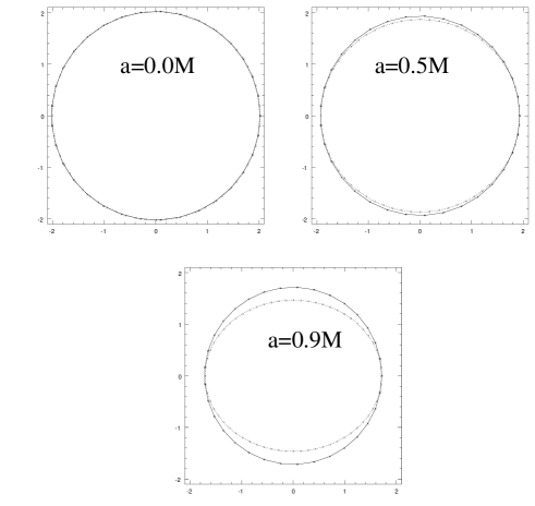
FIG. 7.: The three plots correspond to the location of the apparent horizons for black holes with three different values of angular momentum. The units of the graph are $M$, the solid line is the $\theta=\pi/2$ slice and the dashed line is the $\phi=\pi$ slice.

The radius of the event horizon is given by

$$r_{+}=M+\sqrt{M^{2}-a^{2}}.$$ (36)

The solution to eqn.(36) for $a=0.5M$ is $r_{+}=1.87M$ and the numerical solution we obtain for the horizon radius is $r_{num}=1.87M$, with an error of $0.06\%$. In the $a=0.9M$ case, $r_{+}=1.44M$ and $r_{num}=1.46M$, with a $1.39\%$ error. The area of the horizon for each case can be calculated using

$$A=4\pi(r_{+}^{2}+a^{2})$$ (37)

(generalizing eqn.(30)), and compared to a numerical eqn.(31). computation using eqn.(31). In the $a=0.5M$ case, eqn.(30) gives $A=46.89M^{2}$, numerically we obtain $A_{num}=46.88M^{2}$, resulting in a $0.21\%$ error. In the $a=0.9M$ case, $A=36.09M^{2}$ and $A_{num}=36.39M^{2}$ with a $0.83\%$ error. The errors will decrease as $\kappa$ is driven closer to zero.

C Brill-Lindquist Data

In this section, we study a binary black hole system using Brill-Lindquist data [IX]. These data are useful to us for two reasons: We can verify previous results of the critical separation, and study an example of how the tracker works in finding multiple apparent horizons. The 3-metric is time symmetric, $K_{ab}=0$, and is conformally flat:

$$g_{ab}=\phi^{4}\eta_{ab}$$ (38)

where

$$\phi=1+\sum^{N}_{i=1}\frac{M_{i}}{2r_{i}}$$ (39)

and $N$ is the number of holes (here $N=2$), $M_{i}$ is the mass of the ith black hole and the $r_{i}$ are the radial distances from the centers of the black holes

We use isotropic coordinates to express the metric as

$$ds^{2}=\phi^{4}(dr^{2}+r^{2}d\theta^{2}+r^{2}\sin^{2}\theta d\phi^{2})$$ (40)

with

$$r_{i}=\sqrt{r^{2}+d_{i}^{2}-2d_{i}r\cos\theta},$$ (41)

where $d_{i}$ is the distance between the holes and the center of the coordinate system. When they are far apart, each hole has an apparent horizon of radius $M/2$ in these coordinates. The area of each of the holes when they are well separated is $16\pi M^{2}$.

The limiting separation of the holes between single and double horizons was found by Brill and Lindquist [21] to be $1.56M$, Cadez $1.534M\pm 0.002M$ [22], $[1.5M,1.6M]$ by Alcubierre et al. [23], and $1.535M$ by Huq [13]. We found a critical separation 1.53(5)M. The apparent horizon at the critical separation of 1.535M is shown in fig.(8) using the level flow code with $33^{2}$ grid points.

FIG. 8.: Separation of $1.535M$ with a $33^{2}$ grid. The area was determined numerically to be $184.16M^{2}$

The horizon found for a separation of $d=1.5M$ which is less than the critical separation, is shown in fig.(9). Fig.(10) is a plot of the $l_{2}$-norm of the maximum of $\kappa(\theta)$ for the separation $d=1.5M$ at each iteration plotted versus the number of $\lambda$-steps. This is one of the checks in the level flow code to ensure that the apparent horizon equation is still being solved. We expect the expansion to continue to decrease if we have started outside the apparent horizon and are flowing inward. As we will see in fig.(14), the expansion increases as fission occurs in a data set with separated holes.

FIG. 9.: Separation of $1.5M$ with a $33^{2}$ grid. The area is $185.41M^{2}$.

FIG. 10.: The absolute value of the maximum of expansion, $\kappa$, per iteration, $\lambda$ every 20th step. The kinks at $\lambda=1000$ and $\lambda=2000$ are from restarting the code with a different $\lambda$-step.

As we increase the separation between the two holes to a separation greater than the critical separation, we can test the apparent horizon tracker in the case of multiple apparent horizons. We demonstrate with a separation of $d=2.0M$. The initial surface flows to the point of fissioning where the topology of the surface changes from a one surface into two surfaces. Fig.(11) is a plot of the initial surface that begins the flow. The level set found during this flow is depicted in fig.(12). Each of the surfaces in fig.(12) has a constant expansion, $\kappa=c_{n}$ and was used to indicate a topology change in the test surface. The values for the expansion are $c_{1}=0.14$, $c_{2}=0.12$, $c_{3}=0.1$, and $c_{4}=0.08$. The last single surface just before the topology change is not a surface in the level set; it is plotted in fig.(13). At this point the tracker begins to flow two surfaces.

FIG. 11.: The starting surface of the level flow method for a separation of d=2.0M

FIG. 12.: The level set of surface for the d=2.0M case. Each surface has a constant $\kappa=c_{n}$ at each point. In this case the values for $c_{n}$ are $c_{1}=0.14$, $c_{2}=0.12$, $c_{3}=0.1$, and $c_{4}=0.08$. The level set is used to indicate the change in topology associated with multiple surfaces.

In contrast to a separation of $d=1.5M$ where there is no fission, here as fissioning becomes imminent, the $\kappa$ begins to increase. Fig.(14) is a plot of the absolute value of the maximum across the surface of the expansion, $\kappa$, versus $\lambda$ up to the point of fission. The increase in the expansion is one of the signals of imminent fission. As the algorithm tries to find a surface with $\kappa=0$ everywhere, it is driven into two surfaces. Once the new surfaces are found, the maximum of the expansion begins a monotonic decrease as in fig.(10).

FIG. 13.: The single surface is about to fission into two surfaces.

FIG. 14.: The absolute value of the maximum of expansion, $\kappa$, per iteration is plotted. The increase in the expansion is caused by imminent fission.

The exaggerated peanut shape in fig.(15) and fig.(16) is taken for the same $\lambda$-value as fig.(13).

Once the fissioning is detected by the code, it automatically begins flowing two new surfaces of the same resolution as the parent surface. The series of snapshots shown in fig.(15) and fig.(16) is a subset of the set of surfaces found by the apparent horizon tracker as it follows the fission of the trial surface into two surfaces. The tracker starts with a spherical starting surface that deforms along the gradient field.

FIG. 15.: This series of snapshots depicts the flow of an initial surface until its fission for the binary Brill-Lindquist black holes separated by $2M$. The lower left plot is a first try at determining the final two surfaces. The cusps are due to a typical drawback associated with using points to define the flowing surface. The points crowd together in regions of greater flow. The next snapshot, on the lower right, shows the code’s automatic correction; and shows the apparent horizons of the binary Brill-Lindquist data to an accuracy of $10^{-4}$.

As the points defining the surface flow, the distance between the points can become too small for the finite difference scheme at that resolution. Redistribution of the points on the surface is taken care of automatically by updating the center and radius.

FIG. 16.: The series of pictures shown in fig.(15) are placed in one plot. The outer surface is the initial guess, the “peanut surface” is the surface that is found indicating the need to search for two surfaces, and the inner approximate spheres result from locating the apparent horizons for Brill-Lindquist data.

VII Apparent Horizons in a Grazing Collision

As stated in the Introduction, one of the main motivators of this work is to have an apparent horizon finder that can locate disjoint horizons during the evolution. This entails 1) finding the horizons without a good initial guess, and 2) detecting the topology change from two disjoint horizons to one horizon. To demonstrate the level flow’s ability to carry out 1) and 2), we report the results of apparent horizon tracking in the particular case of a short evolution of two spinning, Kerr-Schild black holes using the Binary Black Hole Grand Challenge Alliance Cauchy code [24]. A future paper [25] will discuss the details of the evolution.

The evolution is free, i.e. the momentum and Hamiltonian constraint equations are only used as checks during the evolution. Since we cannot hold infinity on the grid in this formalism, we must specify outer boundary conditions for the dynamic variables, $g_{ij}$ and $K_{ij}$. For the following work, we specify analytic outer boundary conditions with blending [26] between the analytic and numeric regions.

To specify initial data for two spinning, boosted black holes we use superposed Kerr-Schild black holes. We chose a Kerr-Schild metric [IX] for two reasons: 1) The metric is well defined at the event horizon, and 2) The metric is Lorentz form-invariant in a simple sense, under boosts ($v>0$). The superposed data are constructed in an approximate manner by a conformal method based on the superposition of two isolated, boosted Kerr black holes.

The initial data follows from Matzner et al. [27] and was first implemented by Correll  [28]. The data is the superposition of two, isolated, boosted Kerr-Black holes with individual metrics given by eqn.(23). The resulting superposed metric is:

$$\hat{g}_{ij}={}_{(1)}g_{ij}+{}_{(2)}g_{ij}-\eta_{ij}$$ (42)

with the   $\hat{}$   symbol indicating a quantity conformally related to the physical metric, $g_{ij}=\phi^{4}\hat{g}_{ij}$.

$${}_{(1)}g_{ij} = \eta_{ij}+{}_{(1)}H(r_{1}){}_{(1)}l_{i}{}_{(1)}l_{j}\mbox{\hskip 14.22636pt and}$$ (43)

$${}_{(2)}g_{ij} = \eta_{ij}+{}_{(2)}H(r_{2}){}_{(2)}l_{i}{}_{(2)}l_{j}$$ (44)

are the the isolated Kerr-Schild metric forms with $l_{i}$ and $H$ corresponding to the single black holes. The two holes have comparable masses, $M_{1}\sim M_{2}$, coordinate separation $r_{12}$, and velocities $v_{1}$ and $v_{2}$ assigned to them. For the argument of $H$ and $l_{j}$, we use

$${r_{1}}^{2} = (x-x_{1})^{i}(x-x_{1})^{j}\delta_{ij}\hskip 5.69046pt\mbox{ and}$$ (45)

$${r_{2}}^{2} = (x-x_{2})^{i}(x-x_{2})^{j}\delta_{ij}$$ (46)

with ${x_{1}}^{i}$ and ${x_{2}}^{j}$ the coordinate positions of the holes on the initial slice.

The extrinsic curvatures of the two isolated black holes are added to obtain a trial ${\hat{K}}_{ab}$ for the binary black hole system given as:

$${}_{(0)}{\hat{K}}_{ij}={}_{(1)}{\hat{K}}_{ij}+{}_{(2)}{\hat{K}}_{ij}.$$ (47)

The subscript $0$ indicates that this is an approximation to the true extrinsic curvature of the binary black hole spacetime. ${}_{(1)}{\hat{K}}_{ij}$ and ${}_{(2)}{\hat{K}}_{ij}$ are the individual extrinsic curvatures associated with the isolated Kerr-Schild metric and their indices are raised and lowered by their individual metrics, eqn.(43).

For the data we describe here (holes center initially separated by a coordinate distance exceeding $10M$ where $M$ is the mass of one of the holes), we expect that an initial value solution will be $\approx 10\%$ in error on the domain outside of the excision volume. See further discussion in [29]. We set the lapse function to:

$$\alpha=\alpha_{1}+\alpha_{2}-1,$$

and the shift vector to:

$$\beta^{i}=\beta_{1}^{i}+\beta_{2}^{i}.$$

The run presented in this paper has a grid $81\times 81\times 81$ in Cartesian coordinates $(x,y,z)$ with a domain of $(\pm 10M,\pm 10M,\pm 10M)$ resulting in a spatial resolution of $M/4$. The data represent two black holes in a grazing collision. The holes are set initially at $(5M,1M,0M)$ and $(-5M,-1M,0M)$ in Cartesian coordinates with a boost speed of $\pm 0.5\hat{x}$ toward one another and each has an angular momentum per unit mass of $a=0.5M$ in the $(-)$z-direction. Fig.(17) is the initial configuration of this run; note that a naive sum of the spin and the orbit angular momentum yields zero for this configuration.

We post-process the data obtained from the evolution. For the purposes of this paper, we track the apparent horizons at three specific times during the evolution, namely $t=0M$, $2.8M$, and $3.4M$. At $0M$, the apparent horizons of the initial data are found, at $2.8M$ two disjoint apparent horizons are found; and finally, at $3.4M$ a single apparent horizon is found. For the horizons shown here, the level flow method used a sphere of radius $8M$ to initialize each run. Fig. 18 is a plot of the horizons with time going up the page. The lowest plot is of $t=0M$, with each horizon being a sphere centered at coordinates $(\pm 5M,\pm 1M,0M)$. The middle plot shows the horizons at a later time, $t=2.8M$. Here the deviation in shape as the horizons accelerate towards each other is seen. The final plot at the top of fig. 18 is the first single apparent horizon that envelops both black holes at $t=3.4M$.

The areas for the apparent horizons at $t=0M$ are $A=43.6M^{2}$ for each hole. At $t=2.8M$, the horizons have deviated from a spherical shape and the areas for each hole are $A=44.2M^{2}$, giving a measure of the accuracy to which we can maintain their areas constant. The area of the merged apparent horizon at $t=3.4M$ is $A_{merged}=184M^{2}$. According to the black hole area theorem of Hawking and Ellis [30], the area of the merged event horizon must equal at least the combined area of the individual event horizons. Although no strong statements can be made about the area of an apparent horizon, we do find $A_{merged}>A_{1}+A_{2}$ in a consistent manner. We can further surmise that the final maximum area we could expect based on the initial configuration should be that of a Schwarzschild black hole of mass $2M$, giving an area of approximately $201M^{2}$. In some sense the area predicted by the Schwarzschild case is an upper bound. We see a $8.5\%$ deviation from that “idealized” case. In view of this upper limit, $8.5\%$ may be an indication of the greatest amount of gravitational radiation up to the time of merger ($t=3.4M$) given our approximate initial data, gauge condition, and boundaries.

FIG. 17.: The configuration of the initial data for the grazing collision. The initial mask position is indicated by the “circle” centered on each hole. The angular momentum per unit mass and velocity of each of the holes is also represented. The total angular momentum (spin plus orbit) of the initial configuration is zero.

FIG. 18.: The apparent horizons are plotted with the evolution time increasing up the page. The times plotted are $0.0M$, $2.8M$, and $3.4M$.

VIII Conclusion

Apparent horizon location and tracking constitute an important part of numerical evolutions of black hole spacetimes using excision techniques. We have demonstrated a method for finding apparent horizons in situations where the location of the apparent horizon may not be known; hence a good initial guess for the finder may not be possible. The method we have discussed works with generic 3-metric and extrinsic curvature data and with an arbitrary initial starting surface. Furthermore, the method is capable of detecting a topology change as the finder flows towards the apparent horizon. This ability is important for situations where there are multiple apparent horizons in the data. This allows us to locate apparent horizons in binary black hole evolutions without knowing where the apparent horizons are; and it allows us to locate the first single apparent horizon that forms at the merger of two black holes. The level flow method is successful at locating the apparent horizons in generic spacetimes as demonstrated by the Schwarzschild and Kerr data. It also found multiple apparent horizons starting from a single starting surface as demonstrated with the Brill-Lindquist data. Most importantly, the level flow method has been successful at identifying apparent horizons in a binary black hole evolution involving two Kerr-Schild black holes. Beginning with a single guess surface, two discrete apparent horizons were found at early times, and the later single merged horizon was found.

One of the drawbacks of this method currently is its slow convergence property due to the parabolic nature of the equation solved. This, however does not pose a problem since the level-flow method can be used in conjunction with other methods which may be more efficient given a good initial guess. The level-flow method has the definite advantage of being capable of finding multiple surfaces in the data. It can be used to get extremely good initial guesses for other methods that converge more quickly close to the solution. We are currently using the level flow method in this manner in numerical evolutions of black hole collisions.

IX Acknowledgments

We thank Pablo Laguna for suggesting this topic to DMS, Randy Correll for supplying the initial data routine used in the evolution, and Luis Lehner for discussions on the tracker and evolution. This work was supported by NSF ASC/PHY9318152, NSF PHY9800722, NSF PHY9800725 to the University of Texas and NSF PHY9800970 and NSF PHY9800973 to the Penn State University.

REFERENCES

- [1] J. York, “Kinematics and Dynamics in General Relativity”, Sources of Gravitational Radiation, edited by L. Smarr, Cambridge Univ. Press (1979).
- [2] Seidel, E. and Suen, W., Phys. Rev. Lett 69, 1845 (1992)
- [3] W. Unruh, quoted in J. Thornburg, Class. Quant. Grav., 4, 1119 (1987).
- [4] P. Anninos, K. Camarda, J. Libson, J. Masso, E. Seidel, W-M. Suen, Phys. Rev. D 58 024003 (1998).
- [5] T. Baumgarte, G. Cook, M. Sheel, S. Shapiro, S. Teukolsky, Phys. Rev. D 54 4849-4857 (1996).
- [6] C. Gundlach, Phys. Rev. D 57, 863-875 (1998).
- [7] M.F. Huq, M.W. Choptuik and R.A. Matzner, “Locating Boosted Kerr and Schwarzschild Apparent Horizons”, gr-qc/0002076, Submitted to Phys Rev D.
- [8] A.J. Kemball, N.T. Bishop, “The Numerical Determination of Apparent Horizons”, Class. Quant. Grav. 8, 1361 (1991).
- [9] T. Nakamura, Y. Kojima, K. Oohara, “A Method of Determining Apparent Horizons in Three-Dimensional Numerical Relativity”, Phys. Lett. 106A, (1984).
- [10] P. Diener, N. Jansen, A. Khokhlov and I. Novikov, “Adaptive mesh refinement approach to construction of initial data for black hole collisions,” gr-qc/9905079.
- [11] E. Pasch, SFB 382 Report Number 63 (1997).
- [12] J. Thornburg, “Finding apparent horizons in numerical relativity,” Phys. Rev. D54, 4899 (1996).
- [13] M.F. Huq, “Apparent Horizons in Numerical Spacetimes,” PhD Dissertation, University of Texas, (1996).
- [14] K.P. Tod, Clas. Quant. Grav. 8, L115-L118 (1991).
- [15] D. Bernstein, unpublished notes (1993).
- [16] M. Grayson, The Heat Equation Shrinks Embedded Plane Curves to Round Points, J. Diff. Geom., 26, 285 (1987).
- [17] B. Bruegmann, Int. J. Mod. Phys. D 8 (1999) 85.
- [18] S. Osher, J. Sethian, J. Comp. Phys. 79, 12-49 (1988).
- [19] S.A. Teukolsky, Phys.Rev. D.. 61 087501 (2000).
- [20] C. Misner, K. Thorne, J. Wheeler, Gravitation, W.H. Freeman and Co., New York, (1970).
- [21] D.R. Brill, R.W. Lindquist, Phys. Rev. 131, 471 (1963).
- [22] A. Cadez, Ann. of Phys. 83 (1974) 449-457.
- [23] M. Alcubierre, S. Brandt, B. Bruegmann, C. Gundlach, J. Mosso, E. Seidel and P. Walker, “Test beds and applications for apparent horizon finders in numerical relativity,” gr-qc/9809004.
-
[24]
Binary Black Hole Grand Challenge Alliance, National Science Foundation.
http://www.npac.syr.edu/projects/bh/
- [25] R. Correll et al., in preparation.
- [26] R. Gomez, in Proceedings of “The Grand Challenge Alliance Fall Meeting,” Los Alamos, (1997).
- [27] R. Matzner, M. Huq, D. Shoemaker, Phs. Rev. D 59, 024015 (1999).
- [28] R. Correll, “Numerical evolution of Binary Black Hole Spacetimes,” PhD Dissertation, University of Texas, (1998).
- [29] P. Marronetti et al., Phs. Rev. D in press (2000).
- [30] S. Hawking, G. Ellis, The Large Scale Structure of Space-Time Cambridge University Press, Cambridge (1973).